Uncertainty-Aware Normal-Guided Gaussian Splatting for Surface Reconstruction from Sparse Image Sequences

Abstract

3D Gaussian Splatting (3DGS) has achieved impressive rendering performance in novel view synthesis. However, its efficacy diminishes considerably in sparse image sequences, where inherent data sparsity amplifies geometric uncertainty during optimization. This often leads to convergence at suboptimal local minima, resulting in noticeable structural artifacts in the reconstructed scenes. To mitigate these issues, we propose Uncertainty-aware Normal-Guided Gaussian Splatting (UNG-GS), a novel framework featuring an explicit Spatial Uncertainty Field (SUF) to quantify geometric uncertainty within the 3DGS pipeline. UNG-GS enables high-fidelity rendering and achieves high-precision reconstruction without relying on priors. Specifically, we first integrate Gaussian-based probabilistic modeling into the training of 3DGS to optimize the SUF, providing the model with adaptive error tolerance. An uncertainty-aware depth rendering strategy is then employed to weight depth contributions based on the SUF, effectively reducing noise while preserving fine details. Furthermore, an uncertainty-guided normal refinement method adjusts the influence of neighboring depth values in normal estimation, promoting robust results. Extensive experiments demonstrate that UNG-GS significantly outperforms state-of-the-art methods in both sparse and dense sequences. The code will be open-source.

1 Introduction

High-quality surface reconstruction and novel view synthesis are fundamental tasks in computer vision and robotics, with wide-ranging applications in SLAM, 3D reconstruction, AR/VR, and 3D content generation. Recent advancements in Neural Radiance Fields (NeRF) [21] and 3D Gaussian Splatting (3DGS) [14] have emerged as dominant approaches to these tasks.

NeRF achieves impressive rendering fidelity through implicit scene representations. However, its reliance on ray sampling and volumetric rendering leads to substantial training times, often requiring tens of hours. Although subsequent improvements like Instant-NGP [22] have reduced training time to minutes, the quality of geometric reconstruction remains limited by the implicit representation. 3DGS, conversely, employs an explicit representation using Gaussian point clouds and a differentiable splatting pipeline [39] to enable real-time, high-fidelity rendering and efficient scene representation. Nevertheless, 3DGS primarily relies on photometric loss for optimization. This can result in suboptimal geometric accuracy, as individual Gaussians may not accurately conform to the underlying surface due to photometric consistency constraints and adaptive Gaussian growth strategies. The problem is further compounded in sparse-sequence reconstruction [31], where occlusions, limited viewpoint diversity, and intricate spatial relationships introduce significant geometric uncertainty, thereby exacerbating the degradation of reconstruction quality.

To address these limitations, several approaches have been proposed to enhance the geometric accuracy of 3DGS. SuGaR [10] introduces additional regularization terms to adapt Gaussians for surface reconstruction. DN-Splatter [29] leverages foundation models and prior knowledge to refine reconstruction results. 2DGS [11] represents scenes using 2D Gaussian disks and employs surface normal regularization to constrain geometry. PGSR [4] further incorporates multi-view photometric regularization into the 3DGS optimization framework. While these methods primarily focus on geometric and photometric constraints, recent works [19, 15, 37, 9, 27, 13] have begun to explore uncertainty modeling in related contexts. However, these advancements do not explicitly model uncertainty within the 3DGS framework itself, which limits their effectiveness in accurately capturing geometric details.

To overcome these limitations, we propose Uncertainty-aware Normal-Guided Gaussian Splatting (UNG-GS), the first framework to introduce an explicit Spatial Uncertainty Field that quantifies geometric uncertainty in 3DGS. As shown in Fig. 1, This enables high-fidelity reconstruction and rendering without relying on foundation models or additional priors. Specifically, we embed probabilistic modeling into the online training framework of 3DGS, equipping the model with adaptive error tolerance through a Gaussian negative log-likelihood loss. To suppress noise in uncertain regions, we design an uncertainty-aware rendering strategy that dynamically weights depth rendering based on the spatial uncertainty field. Additionally, an uncertainty-guided adaptive normal refinement strategy refines normal estimation by adaptively weighting neighboring depth gradients. This promotes geometric consistency in low-uncertainty areas and reduces sensitivity to the local planar assumption in high-uncertainty regions like edges.

Our key contributions are summarized as follows:

• We introduce a novel 3D Gaussian Splatting framework, UNG-GS, incorporating an explicit Spatial Uncertainty Field to achieve high-precision reconstruction and high-fidelity rendering without reliance on foundation models or priors;

• We propose an uncertainty-aware rendering strategy that dynamically weights depth rendering based on the spatial uncertainty field, effectively suppressing noise in uncertain regions;

• We design an uncertainty-guided adaptive normal refinement strategy that adaptively weights gradient calculations for robust normal estimation;

• Extensive experiments on Mip-NeRF 360 [3], DTU [12], and TnT [16] datasets demonstrate that UNG-GS significantly outperforms state-of-the-art methods in both sparse and dense sequences.

2 Related Work

2.1 Neural Radiance Fields

NeRF [21] has revolutionized the field of novel view synthesis (NVS) by representing 3D scenes as continuous volumetric functions. NeRF employs a multi-layer perceptron (MLP) to encode both geometry and view-dependent appearance, achieving photorealistic rendering through volume rendering. Subsequent works have extended NeRF in various directions, addressing its limitations in rendering efficiency [22, 7, 28, 17] and geometric accuracy [18, 30, 20, 8, 32, 24, 38]. For instance, Mip-NeRF [2] introduced anti-aliasing techniques to handle multi-scale representations, while Instant-NGP [22] significantly accelerated training through hash-based feature grids. Despite these advancements, NeRF-based methods [18, 8] often struggle with long training times and implicit geometry representations, which limit their ability to produce high-fidelity surface reconstructions. NeuS [30] and VolSDF [32] integrate signed distance functions (SDFs) into the NeRF framework, enabling more accurate surface extraction. However, these methods still rely on implicit representations, which can lead to suboptimal convergence and noisy geometry, particularly when the input images in sequence are sparse. In contrast, our approach, UNG-GS, explicitly models geometric uncertainty and leverages a spatial uncertainty field to achieve high-fidelity surface reconstruction.

2.2 3D Gaussian Splatting

3DGS [14] has emerged as a powerful alternative to NeRF, offering real-time rendering and efficient scene representation through explicit 3D Gaussian primitives. Unlike NeRF, which relies on volumetric rendering, 3DGS utilizes a differentiable splatting pipeline to project 3D Gaussians onto the image plane, achieving high-quality novel view synthesis with significantly faster training times. However, 3DGS faces challenges in accurately representing surfaces due to the volumetric nature of its Gaussian primitives, which can lead to inconsistent geometry across different viewpoints.

Several works have attempted to address these limitations. For instance, SuGaR [10] introduces additional regularization terms to align Gaussians with surfaces, while DN-Splatter [29] leverages foundation models to improve reconstruction quality. 2DGS [11] represents scenes using 2D Gaussian disks and employs surface normal regularization for better surface alignment. GOF [35] extracts the surface by defining an occupancy field exported from the reconstructed 3DGS. RaDe-GS [36] introduces a novel rasterization method for rendering depth and normal maps to improve geometric representation. PGSR [4] designs an unbiased depth estimation rendering method that enables more accurate depth estimation and improves the accuracy of geometric reconstruction by introducing multi-view constraints.

Despite these improvements, existing methods often fail to explicitly model geometric uncertainty, leading to degraded performance in sparse-sequence scenarios. Our UNG-GS framework introduces an explicit Spatial Uncertainty Field to quantify geometric uncertainty, enabling robust surface reconstruction and high-fidelity rendering even with limited input views.

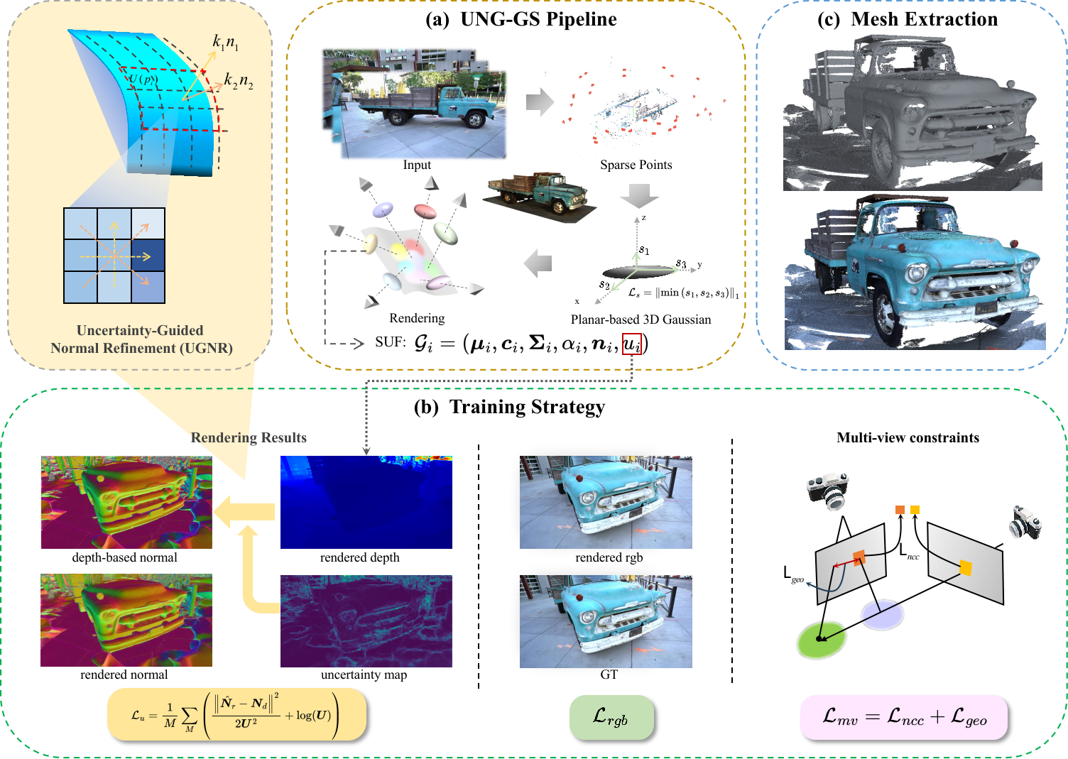
Figure 2: Overview of UNG-GS. Our framework takes sparse image sequence as input, initializes planar-based 3D Gaussians, and proposes a Spatial Uncertainty Field (SUF) to quantify geometric uncertainty. An uncertainty-aware depth strategy dynamically weights depth rendering, while the rendered uncertainty map refines depth-to-normal estimation. High-quality surfaces are extracted via TSDF fusion.

3 Method

Our UNG-GS framework, as illustrated in Fig. 2, introduces an explicit Spatial Uncertainty Field (SUF) to enhance 3D Gaussian Splatting (3DGS) for robust surface reconstruction, particularly from sparse image sequences. We first describe a foundation with planar-based 3D Gaussian Splatting (Section 3.1), rendering color, depth, and normals from the 3D Gaussians. To explicitly model geometric uncertainty, we introduce the Spatial Uncertainty Field (SUF) (Section 3.2), which assigns an uncertainty value to each Gaussian. Next, we leverage SUF in our Uncertainty-aware Geometric Reconstruction module (Section 3.3), which includes Uncertainty-Aware Depth Rendering (UADR) and Uncertainty-Guided Normal Refinement (UGNR) to improve depth and normal estimation, respectively. Finally, the entire framework is trained end-to-end using uncertainty-aware loss functions (Section 3.4) to optimize rendering quality, geometric accuracy, and uncertainty estimation.

3.1 Preliminaries

3.1.1 Planar-based 3D Gaussian Splatting

3DGS represents a scene as a set of 3D Gaussians $\mathcal{G}_{i}$, each defined by its center $\boldsymbol{\mu}_{i}\in\mathbb{R}^{3}$, covariance matrix $\boldsymbol{\Sigma}_{i}\in\mathbb{R}^{3\times 3}$, opacity $\alpha_{i}$, and color $\boldsymbol{c}_{i}$. The covariance matrix is factorized into a scaling matrix $\boldsymbol{S}_{i}$ and a rotation matrix $\boldsymbol{R}_{i}$ as $\boldsymbol{\Sigma}_{i}=\boldsymbol{R}_{i}\boldsymbol{S}_{i}\boldsymbol{S}_{i}^{T}\boldsymbol{R}_{i}^{T}$. The Gaussian is then expressed as:

$$\mathcal{G}_{i}\left(\boldsymbol{x}\mid\boldsymbol{\mu}_{i},\boldsymbol{\Sigma}_{\boldsymbol{i}}\right)=e^{-\frac{1}{2}\left(\boldsymbol{x}-\boldsymbol{\mu}_{i}\right)^{\top}\boldsymbol{\Sigma}_{i}^{-1}\left(\boldsymbol{x}-\boldsymbol{\mu}_{i}\right)}.$$ (1)

They are transformed into the camera coordinate system by:

$$\boldsymbol{\hat{\mu}}_{i}=\boldsymbol{K}\boldsymbol{W}\left[\boldsymbol{\mu}_{i},1\right]^{\top},\quad\boldsymbol{\hat{\Sigma}}_{i}=\boldsymbol{J}\boldsymbol{W}\boldsymbol{\Sigma}_{i}\boldsymbol{W}^{\top}\boldsymbol{J}^{\top},$$ (2)

where $\boldsymbol{W}$, $\boldsymbol{K}$, and $\boldsymbol{J}$ denote the world-to-camera transformation, the camera intrinsic matrix, and the Jacobian of the affine approximation for the projective transformation.

To encourage planar alignment and improve geometric accuracy, we adopt a planar-based Gaussian representation, inspired by [5]. We minimize the smallest singular value of the scaling matrix $\boldsymbol{S}_{i}$ using a regularization term:

$$\mathcal{L}_{s}=\left\|\min\left(s_{1},s_{2},s_{3}\right)\right\|_{1},$$ (3)

where $s_{1}$, $s_{2}$, and $s_{3}$ are the singular values of the scaling matrix $\boldsymbol{S}_{i}$. This regularization encourages Gaussians to flatten along the surface-normal direction, ensuring their centers align closely with the underlying geometry.

3.1.2 Color, Depth, and Normal Rendering

Following typical 3DGS pipelines [14], the rendered color $\boldsymbol{I}$ is obtained via $\alpha$-compositing:

$$\boldsymbol{I}=\sum_{i\in N}T_{i}\hat{\alpha}_{i}\boldsymbol{c}_{i},\quad T_{i}=\prod_{j=1}^{i-1}\left(1-\hat{\alpha}_{j}\right),$$ (4)

where $N$ denotes Gaussians sorted by depth, $T_{i}$ represents the accumulated transmittance, and $\hat{\alpha}$ is calculated by evaluating $\mathcal{G}_{i}\left(\boldsymbol{x}\mid\boldsymbol{\hat{\mu}}_{i},\boldsymbol{\hat{\Sigma}}_{\boldsymbol{i}}\right)$ multiplied with a learnable opacity. Similarly, the rendered normal map $\boldsymbol{\tilde{N}_{r}}$ is generated by blending the normals of the Gaussian planes:

$$\boldsymbol{\tilde{N}_{r}}=\sum_{i\in N}T_{i}\hat{\alpha}_{i}\boldsymbol{R}_{c}^{T}\boldsymbol{n}_{i},$$ (5)

where $\boldsymbol{R}_{c}$ denotes the rotation from the camera to the global world coordinate system. To obtain unbiased depth [4, 26], the distance from the plane to the camera center can be represented as $d_{i}=\left(\boldsymbol{R}_{c}^{T}\left(\boldsymbol{\mu}_{i}-\boldsymbol{O}_{c}\right)\right)\boldsymbol{R}_{c}^{T}\boldsymbol{n}_{i}^{T}$, where $\boldsymbol{O}_{c}$ is the camera center in the world. Then, the distance map $\boldsymbol{Dist}$ and unbiased depth $\boldsymbol{D}$ can be computed as:

$$\boldsymbol{D}=\frac{\boldsymbol{Dist}}{\boldsymbol{\tilde{N}_{r}}\boldsymbol{K}^{-1}\tilde{\boldsymbol{p}}},\quad\boldsymbol{Dist}=\sum_{i\in N}T_{i}\hat{\alpha}_{i}d_{i},$$ (6)

where $\tilde{\boldsymbol{p}}$ denotes the homogeneous coordinates of the pixel.

3.2 Spatial Uncertainty Field (SUF)

With limited input images, such as sparse sequences from a moving camera or restricted coverage scenarios, uncertainty arises from limited viewpoints, occlusions, and noisy depth estimates, leading to ambiguities in localization and surface reconstruction. To explicitly capture this uncertainty, we assign each 3D Gaussian an additional scalar attribute, $u_{i}\in[0,1]$, representing its associated geometric uncertainty. A value of $u_{i}=0$ indicates perfect confidence in the Gaussian’s geometry, while $u_{i}=1$ signifies maximum uncertainty. Similar to color and depth, we render the uncertainty map $\boldsymbol{U}$ by alpha-compositing the uncertainty values:

$$\boldsymbol{U}=\sum_{i\in N}T_{i}\hat{\alpha}_{i}u_{i},$$ (7)

To effectively train and optimize SUF, we propose an uncertainty normal loss, formulated as a Gaussian Negative Log-Likelihood (NLL) loss:

$$\mathcal{L}_{u}=\frac{1}{M}\sum_{M}\left(\frac{\left\|\boldsymbol{\hat{N}}_{r}-\boldsymbol{\hat{N}}_{d}\right\|^{2}}{2\boldsymbol{U}^{2}}+\log(\boldsymbol{U})\right),$$ (8)

where $\boldsymbol{\hat{N}}_{r}$ is the rendered normal map, $\boldsymbol{\hat{N}}_{d}$ is the depth-based normal map, and $i$ indexes the image pixels. The Gaussian NLL loss [23, 1] is chosen because it inherently captures the probabilistic nature of uncertainty estimation. The loss function penalizes deviations between the predicted uncertainty ($U_{i}$) and the actual error in the normal estimation ($\left\|\boldsymbol{\hat{N}}_{r,i}-\boldsymbol{N}_{d,i}\right\|^{2}$). The first term in Equation 8 penalizes large normal discrepancies when the predicted uncertainty is low, encouraging the optimization process to increase the uncertainty for Gaussians with inaccurate normals. Conversely, the $\log(U_{i})$ term acts as a regularizer, preventing excessive uncertainty values and maintaining confidence in regions with accurate normals. This balance is crucial for achieving robust and reliable uncertainty estimation, allowing the framework to effectively distinguish between regions of high and low geometric confidence.

3.3 Uncertaity-Aware Geometric Reconstruction

Uncertainty-Aware Depth Rendering (UADR).

To enhance depth rendering with SUF, we propose an uncertainty-aware depth rendering strategy. It adjusts each Gaussian’s contribution to the final depth using a novel Confidence Modulation Function (CMF), which dynamically incorporates the associated uncertainty values by:

$$w_{i}=-0.5u_{i}^{2}+1.$$ (9)

This quadratic CMF has multiple desirable properties. First, it provides a smooth transition between high-confidence and high-uncertainty regions. When $u_{i}=0$ (high confidence), $w_{i}=1$, preserving the original depth contribution. As $u_{i}$ increases, $w_{i}$ smoothly decreases, progressively suppressing the contribution of uncertain Gaussians. The gradient of the CMF with respect to the uncertainty is given by $\frac{\mathrm{d}w_{i}}{\mathrm{d}u_{i}}=-u_{i}$. This linear gradient ensures stable optimization by preventing abrupt changes in the weights, particularly in regions where the uncertainty is high. Furthermore, the CMF ensures that even highly uncertain Gaussians ($u_{i}=1$) retain a non-negligible weight ($w_{i}=0.5$), preventing complete information loss and allowing for potential recovery during subsequent optimization steps. Compared to alternative modulation functions (a: $w=\exp(-2u)$ and b: $w=(1-u)^{0.1}$), which are evaluated in the experiments, our quadratic CMF offers a superior balance between noise suppression, detail preservation, and optimization stability. The uncertainty-aware rendered depth is computed as:

$$\boldsymbol{D_{u}}=\sum_{i\in N}T_{i}\hat{\alpha}_{i}d_{i}w_{i}.$$ (10)

This ensures that Gaussians with low uncertainty (high confidence) contribute more significantly to the final depth. In contrast, those with high uncertainty (low confidence) are suppressed, effectively reducing noise in uncertain regions.

Uncertainty-Guided Normal Refinement (UGNR).

To enhance the robustness of depth-based normal estimation, we introduce an uncertainty-guided normal refinement strategy. Specifically, we compute two sets of cross products from neighboring depth gradients:

$$\boldsymbol{n}_{1}=\nabla_{x}\boldsymbol{D}_{u}\times\nabla_{y}\boldsymbol{D}_{u},\quad\boldsymbol{n}_{2}=\nabla_{d1}\boldsymbol{D}_{u}\times\nabla_{d2}\boldsymbol{D}_{u},$$ (11)

where $\nabla_{x}$ and $\nabla_{y}$ are the horizontal and vertical gradients of the depth map, $\nabla_{d1}$ and $\nabla_{d2}$ are the gradients along the two diagonal directions. The final refined depth-based normal $\boldsymbol{\hat{N}}_{d}$ is computed as a weighted average of $\boldsymbol{n_{1}}$ and $\boldsymbol{n_{2}}$:

$$\boldsymbol{\hat{N}}_{d}=\frac{k_{1}\boldsymbol{n}_{1}+k_{2}\boldsymbol{n}_{2}}{\left\|k_{1}\boldsymbol{n}_{1}+k_{2}\boldsymbol{n}_{2}\right\|},\quad k_{i}=\sum_{p_{i}\in\mathcal{P}}(1-\boldsymbol{U}(p_{i})),$$ (12)

where the weight $k_{i}$ is determined by the uncertainty values of the pixels involved in the gradient calculations, $\mathcal{P}$ is the set of pixels used to compute $\boldsymbol{n}_{i}$, and $\boldsymbol{U}(p_{i})$ denotes the uncertainty value at pixel $p_{i}$. This weighting scheme ensures that regions with lower uncertainty contribute more to the final normal estimation, enhancing robustness in high-uncertainty areas such as edges.

3.4 Training Functions

To effectively train UNG-GS, our exploit four key loss functions: RGB loss, multi-view consistency loss, scale regularization, and uncertainty normal loss.

RGB Loss

To account for variations in image brightness caused by changing external lighting conditions over time, we incorporate an exposure model into the training procedure. By computing the exposure coefficients $m_{i}$ and $b_{i}$, we obtain the $i$-th exposure-compensated image: $\boldsymbol{I}_{i}^{e}=\exp\left(m_{i}\right)\boldsymbol{I}_{i}+b_{i}$. To ensure structural similarity, the final RGB loss is formulated as:

$$\mathcal{L}_{rgb}=(1-\lambda)\mathcal{L}_{1}\left({\tilde{\boldsymbol{I}^{e}}}-\boldsymbol{\hat{I}}\right)+\lambda\mathcal{L}_{SSIM}\left(\boldsymbol{I}-\boldsymbol{\hat{I}}\right),$$ (13)

where $\tilde{\boldsymbol{I}^{e}}$ is the rendered image adjusted by the exposure coefficients. If the SSIM difference is less than 0.5, the original rendered image is used directly: $\tilde{\boldsymbol{I}^{e}}=\boldsymbol{I}$. $\boldsymbol{\hat{I}}$ denotes the input image, $\mathcal{L}_{1}$ denotes the L1 loss constraint, and $\mathcal{L}_{SSIM}$ denotes the SSIM loss. $\lambda$ is set to 0.2.

Multi-View Consistency Loss

In the case of sparse image sequences, COLMAP [25] generates only a sparse initial point cloud. When relying solely on the single-view constraint, the optimization process may suffer from inconsistency issues during training. To address this problem and enhance the reconstruction quality, we introduce multi-view consistency constraints based on planar patches:

$$\tilde{\boldsymbol{p}}_{n}=\boldsymbol{H}_{rn}\tilde{\boldsymbol{p}}_{r},\quad\boldsymbol{H}_{rn}=\boldsymbol{K}_{r}\left(\boldsymbol{R}_{rn}-\frac{\boldsymbol{T}_{rn}\boldsymbol{n}_{r}^{T}}{d_{r}}\right)\boldsymbol{K}_{r}^{-1},$$ (14)

where $\tilde{\boldsymbol{p}}_{r}$ and $\tilde{\boldsymbol{p}}_{n}$ are the correspondences, $\boldsymbol{H}_{rn}$ and $\boldsymbol{T}_{rn}$ are the homography and transformation from the reference frame to the neighboring frame, respectively.

The multi-view consistency loss $\mathcal{L}_{mv}$ consists of two components: the multi-view photometric constraint $\mathcal{L}_{ncc}$ and the multi-view geometric consistency constraint $\mathcal{L}_{geo}$. Photometric consistency is ensured by minimizing NCC [34] between the reference and adjacent views:

$$\mathcal{L}_{ncc}=\frac{1}{|\mathbb{V}|}\sum_{\boldsymbol{p}_{r}\in\mathbb{V}}\left(1-NCC\left(I\left(\boldsymbol{p}_{r}\right),I\left(\boldsymbol{H}_{nr}\boldsymbol{p}_{n}\right)\right)\right),$$ (15)

where $\mathbb{V}$ denotes the valid region. Geometric consistency is achieved by minimizing reprojection errors:

$$\mathcal{L}_{geo}=\frac{1}{|\mathbb{V}|}\sum_{\boldsymbol{p}_{r}\in\mathbb{V}}\left\|\tilde{\boldsymbol{p}}_{r}-\boldsymbol{H}_{nr}\boldsymbol{H}_{rn}\tilde{\boldsymbol{p}}_{r}\right\|,$$ (16)

and the combined multi-view consistency loss is:

$$\mathcal{L}_{mv}=\mathcal{L}_{ncc}+\mathcal{L}_{geo},$$ (17)

Total Loss

In summary, our complete training loss is:

$$\mathcal{L}=\mathcal{L}_{rgb}+\lambda_{1}\mathcal{L}_{u}+\lambda_{2}\mathcal{L}_{s}+\mathcal{L}_{mv},$$ (18)

where $\lambda_{1}$ and $\lambda_{2}$ weigh the importance of the uncertainty and scaling regularization term, respectively.

4 Experiments

	24	37	40	55	63	65	69	83	97	105	106	110	114	118	122	Mean	Time
2D GS [11]	1.19	1.06	1.22	0.64	1.38	1.20	1.01	1.27	1.22	0.68	1.09	1.86	0.50	0.87	0.58	1.05	9.6m
GOF [35]	0.81	1.10	0.81	0.46	1.36	1.11	0.82	1.21	1.41	0.61	1.05	1.33	0.49	0.88	0.64	0.94	1h
RaDe-GS [36]	0.74	1.15	1.06	0.44	0.95	1.02	0.78	1.20	1.22	0.65	0.86	0.89	0.40	0.92	0.57	0.86	8m
PGSR [4]	0.72	0.86	0.75	0.67	0.81	0.70	0.56	1.06	1.00	0.59	0.63	0.51	0.31	0.38	0.36	0.66	0.5h
Ours	0.64	0.82	0.63	0.43	0.80	0.74	0.53	1.05	0.99	0.58	0.54	0.51	0.30	0.35	0.35	0.62	25m

Table 1: Quantitative comparison on the DTU Dataset [12]. We report the Chamfer Distance (CD) [mm$\downarrow$] and our method achieves the best performance among all GS-based methods.  ,  ,   indicate the best, the second best, and the third best respectively.

	2D GS [11]	GOF [35]	RaDe-GS [36]	PGSR [4]	Ours
Barn	0.34	0.29	0.30	0.34	0.43
Caterpillar	0.26	0.27	0.28	0.31	0.35
Courthouse	0.18	0.23	0.24	0.08	0.24
Ignatius	0.45	0.50	0.55	0.61	0.63
Meetingroom	0.03	0.11	0.10	0.10	0.12
Truck	0.39	0.32	0.33	0.52	0.56
Mean	0.28	0.29	0.30	0.33	0.39
Time	15m	>1h	23m	1.1h	40m

Table 2: Quantitative comparison on the TnT Dataset [16]. We report the F1-score and average optimization time. All results are evaluated with the official evaluation scripts. Our method achieves the best score among Gaussian Splatting methods.

	Outdoor Scene			Indoor scene
	PSNR $\uparrow$	SSIM $\uparrow$	LPIPS $\downarrow$	PSNR $\uparrow$	SSIM $\uparrow$	LIPPS $\downarrow$
NeRF [21]	21.46	0.458	0.515	26.84	0.790	0.370
Instant NGP [22]	22.90	0.566	0.371	29.15	0.880	0.216
MipNeRF360 [3]	24.47	0.691	0.283	31.72	0.917	0.180
3DGS [14]	24.64	0.731	0.234	30.41	0.920	0.189
SuGaR [10]	22.93	0.629	0.356	29.43	0.906	0.225
2D GS [11]	24.34	0.717	0.246	30.40	0.916	0.195
PGSR [4]	24.45	0.730	0.224	30.41	0.930	0.161
Ours	24.79	0.751	0.199	30.57	0.932	0.153

Table 3: Quantitative results on Mip-NeRF 360 [3] dataset.

4.1 Experimental Setup

Datasets.

To evaluate our method, we conduct experiments on the Tanks & Temples (TnT) [16], DTU [12], and Mip-NeRF360 [3] datasets. We simulate sparse image sequence reconstruction by downsampling the TnT and DTU datasets. For TnT, we retain one frame every eight frames, and for DTU, one frame every four frames. Sparse point clouds and camera poses are then generated using COLMAP [25]. This approach aligns with real-world scenarios where image sequences are often sparse and irregularly sampled. In contrast, Mip-NeRF 360 is designed to evaluate rendering performance rather than reconstruction accuracy, so we use a standard dataset.

Implementation.

We design a novel uncertainty-aware differentiable rasterization module, implemented in CUDA, which generalizes and enhances the capabilities of 3DGS and PGSR by explicitly modeling uncertainty in the rendering process. We employ AbsGS’s [33] densification strategy and extract meshes via TSDF Fusion [6]. Our training strategy has three stages: (1) only photometric loss and scale regularization before 15,000 iterations; (2) uncertainty normal loss and multi-view constraints to optimize spatial uncertainty field (SUF) and geometry from iteration 15,000; and (3) UGNF starting at iteration 20,000 for enhanced geometric quality.

Evaluations.

We compare our method with SOTA Gaussian Splatting methods, including 2DGS [11], GOF [35], RaDe-GS [36], and PGSR [4], for surface reconstruction and rendering performance. Due to the computational intensity of NeRF-based methods [21, 30, 8, 32], we provide dense sequence results in the discussion and supplement for comparison. We evaluate reconstruction quality by following baselines [11, 35, 36, 4] using Chamfer Distance (CD) on the DTU dataset and F1-score on the TnT dataset. For novel view synthesis, we employ PSNR, SSIM, and LPIPS as evaluation metrics.

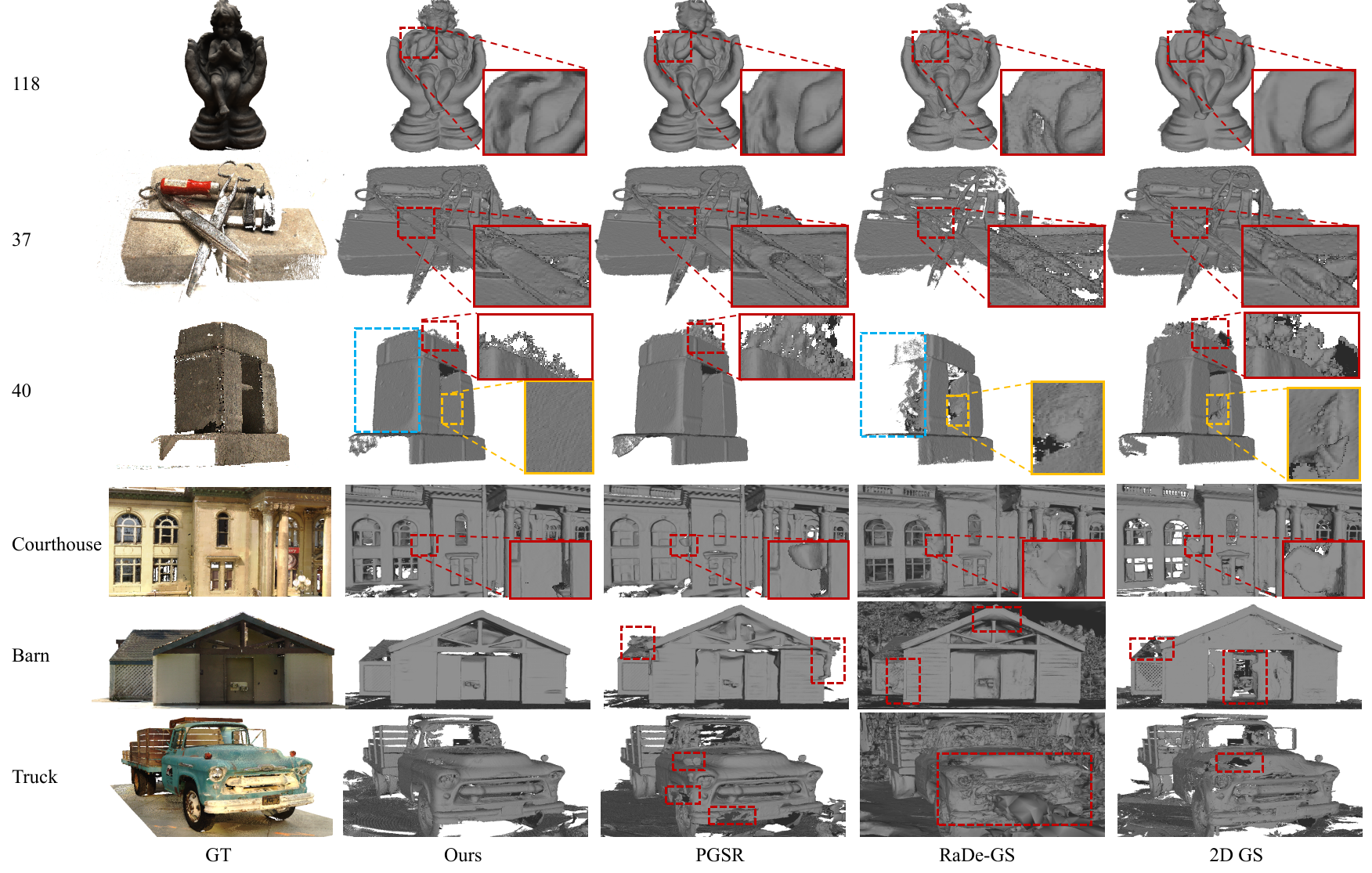
Figure 3: The qualitative comparisons of surface reconstruction on the DTU [12] and TnT [16] datasets. Our method produces smoother and more detailed surfaces under sparse-sequence compared to existing GS-based methods [4, 36, 11].

4.2 Results Analysis

Reconstruction Performance.

We compare our method with existing methods on the DTU and TnT datasets in Tab. 1 and Tab. 2. On the DTU dataset, our method achieves state-of-the-art reconstruction accuracy, as quantified by an average CD of 0.62, while maintaining a relatively efficient optimization time of 25 minutes. Compared to existing approaches, our method significantly improves in reconstruction accuracy, ranging from 6.1% to 41.0%. Furthermore, on the TnT dataset, our method attains state-of-the-art reconstruction quality, yielding an average F1-score of 0.39, with a competitive optimization time of 40 minutes. Compared to other methods, the reconstruction quality is improved ranging from 18.2% to 39.3%. This indicates that our method achieves a better balance between the accuracy of geometric reconstruction and computational efficiency.  Fig. 3 presents a qualitative comparison with existing GS-based methods on DTU and TnT datasets and our method achieves higher-quality results.

Rendering Performance.

To evaluate rendering performance, we compare our method with existing methods on the Mip-NeRF 360 [3] dataset. The results presented in Tab. 3 show that our approach can also improve the rendering quality in the novel view synthesis task.

4.3 Ablation Studies

Metric	w/o UGNR	w/o UADR	w/o SUF	full model
F1-Score $\uparrow$	0.535	0.530	0.521	0.560

Table 4: Reconstruction quality study on the TnT Truck.

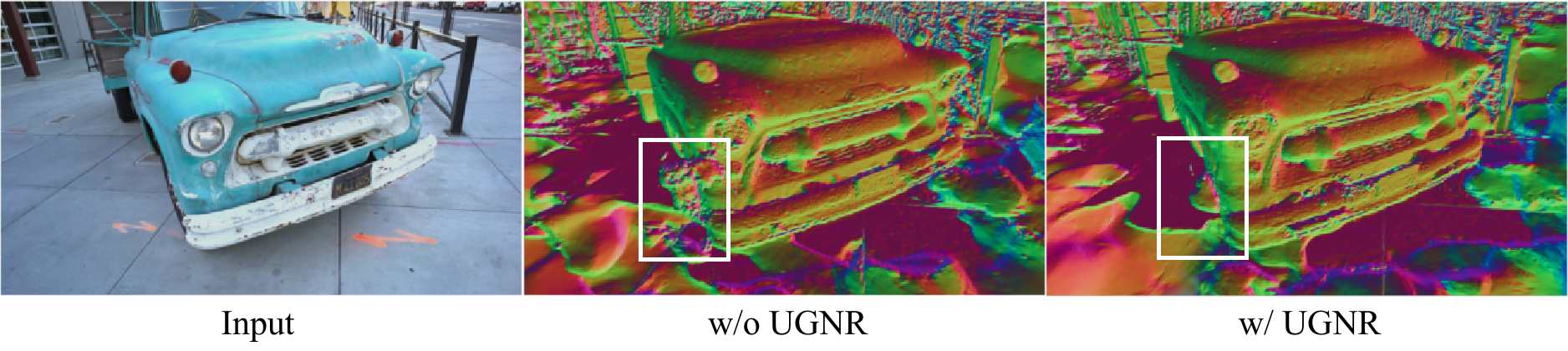
Figure 4: Ablation study of UGNR. We compare the differences in rendered normal images generated during training with and without UGNR after 10000 iterations.

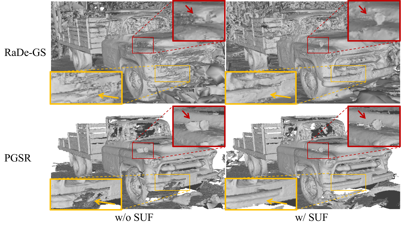
Figure 5: Generalizability of the SUF. We added our proposed SUF to the normal-guided methods PGSR [4] and RaDe-GS [36] for verification and found that SUF can better reconstruct edge features and is not prone to losing details.

Metric	PGSR [4]		RaDe-GS [36]
	w/o SUF	w/ SUF	w/o SUF	w/ SUF
F1-Score $\uparrow$	0.521	0.543	0.329	0.346

Table 5: Generalizability of the SUF. We added SUF to the normal-guided methods PGSR and RaDe-GS to verify the effectiveness and generalization of our proposed framework.

Components Analysis.

Table 4 presents a quantitative analysis of the impact of key components of our UNG-GS framework on reconstruction performance. Specifically, we evaluate the contribution of SUF, UADR, and UGNR modules by systematically removing each component from the full UNG-GS pipeline. The results, obtained on the TnT dataset (scene: Truck), demonstrate that ablating any of these components leads to a degradation in reconstruction accuracy, highlighting the importance of their synergistic integration. Notably, the removal of the SUF results in the most significant performance drop, indicating its critical role in geometric uncertainty modeling, while ablating UGNR has the least impact, suggesting that its contribution is more nuanced and potentially dependent on other factors.

Generalizability of the SUF.

To assess the generalization ability of the proposed SUF, we conducted experiments wherein we integrated our SUF module into two existing normal-guided surface reconstruction methods: PGSR [4] and RaDe-GS [36]. We modified the publicly available CUDA implementations of these methods, incorporating the SUF and retraining the models. As shown in Table 5 and visualized in Fig. 5, the incorporation of the SUF consistently improved reconstruction accuracy for both PGSR and RaDe-GS. These results indicate that the underlying principle of explicitly modeling geometric uncertainty through a probabilistic framework, as embodied by the SUF, possesses a degree of generalizability and can be effectively integrated into diverse surface reconstruction pipelines to enhance their performance.

Metric	(a)  $\exp(-2u)$	(b)  $(1-u)^{0.1}$	Ours
F1-Score $\uparrow$	0.483	0.520	0.560

Table 6: Ablation study of uncertainty-aware depth rendering strategies. We compare results on the Truck scene.

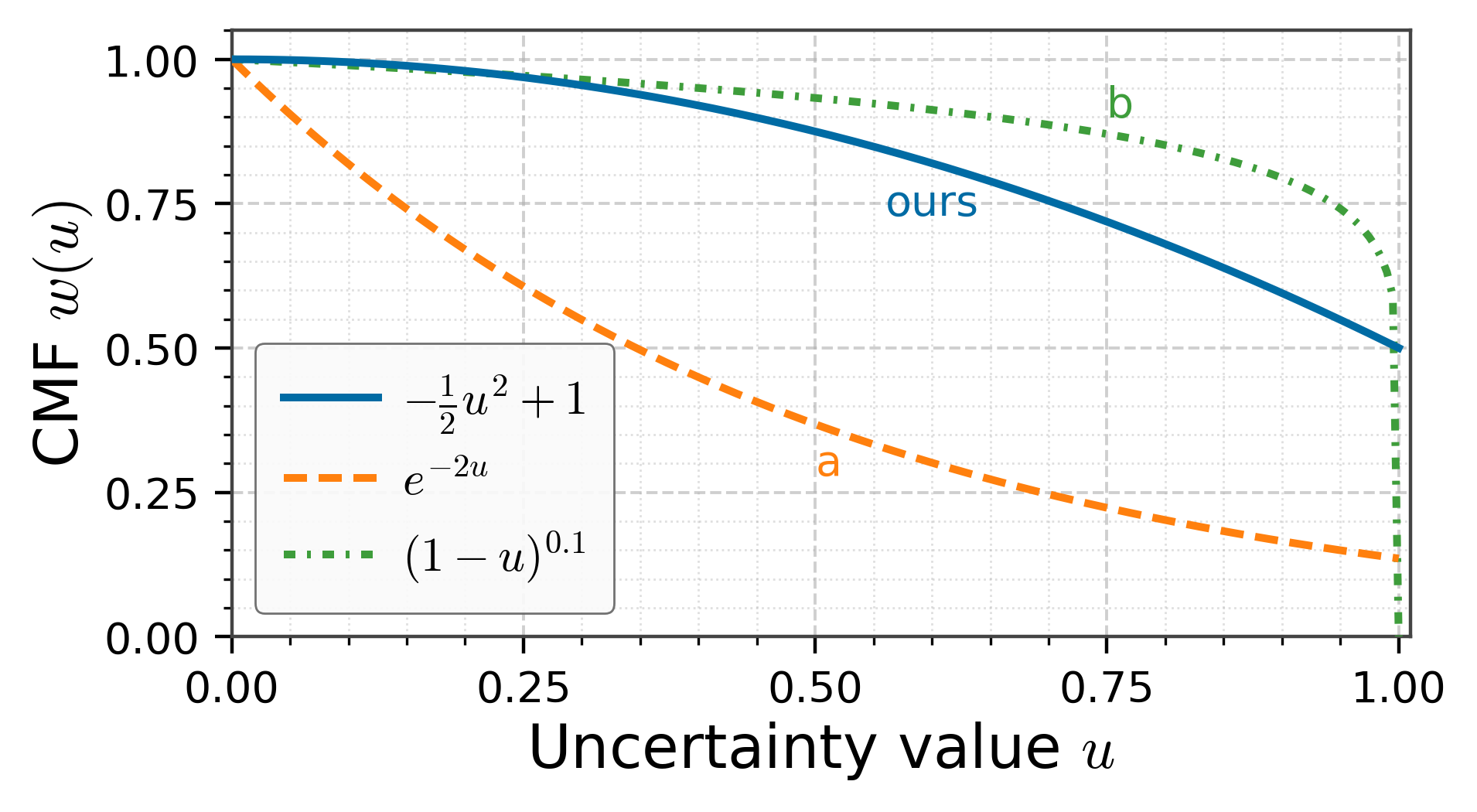
Figure 6: Comparison of different CMFs.

Impact of CMF Design.

In this experiment, we compared two alternative CMFs: (a) $w=\exp(-2u)$ and (b) $w=(1-u)^{0.1}$. As shown in Table 6, our CMF yields significantly improved performance compared to the other two functions. As illustrated in Fig. 6, the superior performance can be attributed to the linear gradient of our designed CMF. As $u$ increases, the gradient smoothly transitions from 0 to -1, promoting stability during the optimization process and mitigating the risk of training instability or convergence issues caused by abrupt gradient changes. In contrast, CMF (a) exhibits a faster gradient change, particularly when $u$ approaches 0, potentially leading to overly rapid weight updates and affecting stability. CMF (b), on the other hand, displays a very steep gradient when $u$ is close to 1, which can induce gradient explosion or unstable optimization behavior. Furthermore, our CMF retains appropriate weight values even in low-confidence regions, effectively suppressing noise while preserving valuable information, thereby leading to improved performance from sparse image sequences.

	3D GS	SuGaR	2D GS	GOF	RaDe-GS	PGSR	Ours
	[14]	[10]	[11]	[35]	[36]	[4]
DTU (CD $\downarrow$ [mm])	1.96	1.33	0.80	0.74	0.68	0.53	0.51
TnT (F1-score $\uparrow$)	0.09	0.19	0.30	0.34	0.37	0.50	0.51

Table 7: Quantitative comparison of dense image sequence on the DTU [12] and TnT Dataset [16].

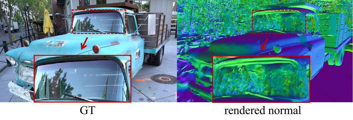
Figure 7: Glass mirror reflection reconstruction failed.

Discussion & Limitations.

UNG-GS achieves significant improvements in sparse-view reconstruction and further demonstrates consistent performance gains in dense-view scenarios compared to SOTA methods, as shown in Table 7. This indicates that the proposed SUF and related strategies not only excel in sparse-view conditions but also enhance reconstruction quality when data is abundant, highlighting the generalizability of our approach. However, as shown in Fig. 7, UNG-GS may still face challenges with highly reflective and transparent surfaces, such as those found in mirrors and glass. Future work could explore incorporating additional priors or specialized rendering methods to better handle these complex materials.

5 Conclusion

This paper presents UNG-GS, a novel framework for high-fidelity surface reconstruction and novel view synthesis from sparse image sequences without priors. By explicitly modeling geometric uncertainty through a normal-guided Spatial Uncertainty Field, UNG-GS tackles the limitations of existing 3DGS methods, which suffer from degraded reconstruction quality due to the lack of uncertainty quantification. Our key innovation lies in embedding probabilistic modeling into the 3DGS framework, enabling adaptive error tolerance during optimization. The proposed uncertainty-aware rendering strategy dynamically suppresses noise in uncertain regions while preserving details in high-confidence areas, and the uncertainty-guided adaptive normal refinement robustly aligns surface normals by adjusting neighborhood gradient weights. Extensive experiments on public datasets demonstrate UNG-GS’s superiority over state-of-the-art methods.

Appendix A Appendix Section

The supplementary materials are organized into two main sections: Additional Implementation (see Section A.1) and Additional Results (see Sec. A.2). It provides additional details and insights into our research, enhancing the transparency and depth of our findings.

A.1 Additional Implementation

Our experiments are conducted on the NVIDIA RTX 4090 GPU, with the uncertainty learning rate set to 0.0025. On the TnT dataset, we use $\lambda_{1}$ = 0.008, while on the DTU dataset, $\lambda_{1}$ = 1e-5. The $\lambda_{2}$ is set to 100. Our training strategy on the DTU dataset involved introducing multi-view and uncertainty losses at iteration 8000. We adopt a similar strategy to [4] for constructing the image graph and selecting adjacent frames, ensuring effective spatial relationships between views.

	24	37	40	55	63	65	69	83	97	105	106	110	114	118	122	Mean
3D GS [14]	2.14	1.53	2.08	1.68	3.49	2.21	1.43	2.07	2.22	1.75	1.79	2.55	1.53	1.52	1.50	1.96
SuGaR [10]	1.47	1.33	1.13	0.61	2.25	1.71	1.15	1.63	1.62	1.07	0.79	2.45	0.98	0.88	0.79	1.33
2D GS [11]	0.48	0.91	0.39	0.39	1.01	0.83	0.81	1.36	1.27	0.76	0.70	1.40	0.40	0.76	0.52	0.80
GOF [35]	0.50	0.82	0.37	0.37	1.12	0.74	0.73	1.18	1.29	0.68	0.77	0.90	0.42	0.66	0.49	0.74
RaDe-GS [36]	0.46	0.73	0.33	0.38	0.79	0.75	0.76	1.19	1.22	0.62	0.70	0.78	0.36	0.68	0.47	0.68
PGSR [4]	0.34	0.58	0.29	0.29	0.78	0.58	0.54	1.01	0.73	0.51	0.49	0.69	0.31	0.37	0.38	0.53
Ours	0.34	0.55	0.36	0.34	0.77	0.57	0.49	1.04	0.63	0.58	0.47	0.51	0.30	0.36	0.33	0.51

Table 8: Quantitative comparison on the standard DTU Dataset [12]. We report the Chamfer Distance (CD) [mm$\downarrow$] and our method achieves the best performance among all GS-based methods.  ,  ,   indicate the best, the second best, and the third best respectively.

	3D GS [14]	SuGaR [10]	2D GS [11]	GOF [35]	RaDe-GS [36]	PGSR [4]	Ours
Barn	0.13	0.14	0.36	0.37	0.43	0.66	0.67
Caterpillar	0.08	0.16	0.23	0.21	0.26	0.41	0.42
Courthouse	0.09	0.08	0.13	0.11	0.11	0.21	0.21
Ignatius	0.04	0.33	0.44	0.63	0.73	0.80	0.81
Meetingroom	0.01	0.15	0.16	0.23	0.17	0.29	0.33
Truck	0.19	0.26	0.26	0.50	0.53	0.60	0.63
Mean	0.09	0.19	0.30	0.34	0.37	0.50	0.51

Table 9: Quantitative comparison on the standard TnT Dataset [16]. We report the F1-score and average optimization time. All results are from the original paper. Our method achieves the best score among Gaussian Splatting methods.

Metric	w/o exposure compensation	w/o mvs-ncc	w/o mvs-geo	w/o UGNR	w/o UADR	w/o SUF	full model
F1-Score $\uparrow$	0.522	0.371	0.497	0.535	0.530	0.521	0.560

Table 10: Ablation study of different components including losses and strategies on the TnT (scene: Truck).

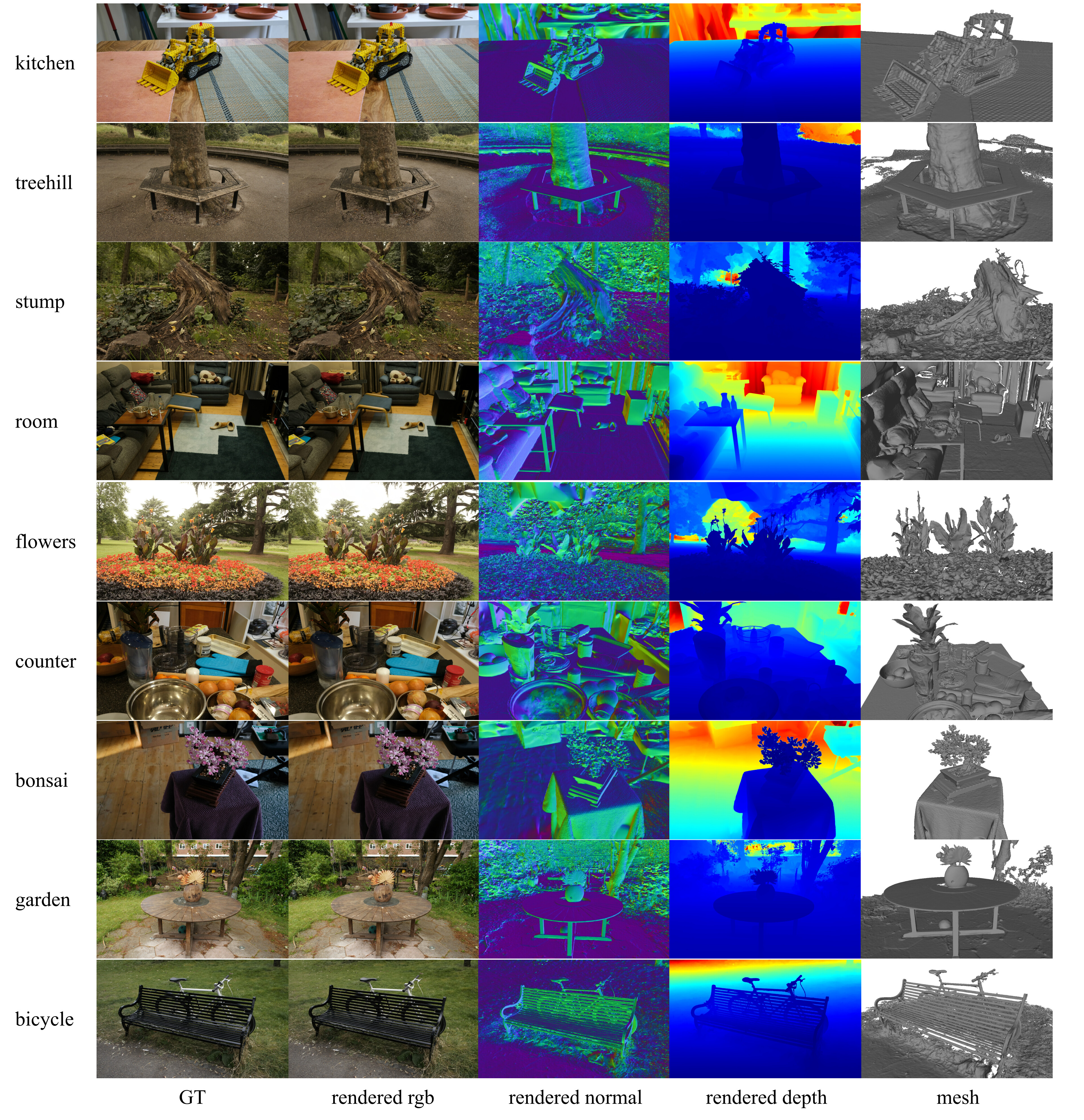
Figure 8: Qualitative results on Mip-NeRF 360 [3] dataset. Our approach can generate high-quality meshes and images including RGB, normal, and depth.

A.2 Additional Results

Reconstruction from Dense Image Sequences.

To further validate the effectiveness of our method, we conducted experiments on dense image sequences using the standard DTU and TnT datasets. Our results show that our approach slightly outperforms state-of-the-art methods in these scenarios. As illustrated in Table 8, our method achieves a Chamfer Distance (CD) of 0.51 mm on the DTU dataset. Similarly, Table 9 demonstrates a slight improvement on the TnT dataset.

The modest improvement in dense image sequences can be primarily attributed to the increased overlapping regions in these datasets. This increased overlap has two key effects: Enhanced Geometric Consistency and Reduced Uncertainty.

• Enhanced Geometric Consistency: More overlap facilitates maintaining geometric consistency across views, which is essential for accurate reconstruction. However, the baseline performance is already high due to the dense nature of the data, limiting the scope for significant improvement.

• Reduced Uncertainty: The abundance of overlapping data reduces overall uncertainty, making explicit uncertainty modeling less critical. As a result, while our method still offers improvements, they are less pronounced compared to sparse sequences.

Qualitative Results on Mip-NeRF 360.

We also evaluated our method on the Mip-NeRF 360 dataset to demonstrate its capability in both rendering and geometric reconstruction. As shown in Fig. 8 The qualitative results include visualizations of RGB images, depth maps, normal maps, and mesh outputs. These visualizations showcase our method’s ability to balance rendering quality with geometric accuracy, providing comprehensive insights into the reconstructed scenes.

Additional Detailed Ablation Study.

To thoroughly assess the contributions of each component in our framework, we conducted an extensive ablation study. The results are presented in Table 10, which highlights the impact of different loss functions and strategies on the overall performance. This analysis confirms the necessity of each design choice in our framework, underscoring the importance of carefully selected loss functions and optimization strategies for achieving optimal results.

References

- Barron [2019] Jonathan T Barron. A general and adaptive robust loss function. In CVPR, pages 4331–4339, 2019.
- Barron et al. [2021] Jonathan T Barron, Ben Mildenhall, Matthew Tancik, Peter Hedman, Ricardo Martin-Brualla, and Pratul P Srinivasan. Mip-nerf: A multiscale representation for anti-aliasing neural radiance fields. In ICCV, pages 5855–5864, 2021.
- Barron et al. [2022] Jonathan T Barron, Ben Mildenhall, Dor Verbin, Pratul P Srinivasan, and Peter Hedman. Mip-nerf 360: Unbounded anti-aliased neural radiance fields. In CVPR, pages 5470–5479, 2022.
- Chen et al. [2024] Danpeng Chen, Hai Li, Weicai Ye, Yifan Wang, Weijian Xie, Shangjin Zhai, Nan Wang, Haomin Liu, Hujun Bao, and Guofeng Zhang. Pgsr: Planar-based gaussian splatting for efficient and high-fidelity surface reconstruction. arXiv preprint arXiv:2406.06521, 2024.
- Chen et al. [2023] Hanlin Chen, Chen Li, and Gim Hee Lee. Neusg: Neural implicit surface reconstruction with 3d gaussian splatting guidance. arXiv preprint arXiv:2312.00846, 2023.
- Curless and Levoy [1996] Brian Curless and Marc Levoy. A volumetric method for building complex models from range images. In Proceedings of the 23rd annual conference on Computer graphics and interactive techniques, pages 303–312, 1996.
- Fridovich-Keil et al. [2022] Sara Fridovich-Keil, Alex Yu, Matthew Tancik, Qinhong Chen, Benjamin Recht, and Angjoo Kanazawa. Plenoxels: Radiance fields without neural networks. In CVPR, pages 5501–5510, 2022.
- Fu et al. [2022] Qiancheng Fu, Qingshan Xu, Yew-Soon Ong, and Wenbing Tao. Geo-neus: Geometry-consistent neural implicit surfaces learning for multi-view reconstruction. NeurIPS, 2022.
- Goli et al. [2024] Lily Goli, Cody Reading, Silvia Sellán, Alec Jacobson, and Andrea Tagliasacchi. Bayes’ rays: Uncertainty quantification for neural radiance fields. In CVPR, pages 20061–20070, 2024.
- Guédon and Lepetit [2023] Antoine Guédon and Vincent Lepetit. Sugar: Surface-aligned gaussian splatting for efficient 3d mesh reconstruction and high-quality mesh rendering. arXiv preprint arXiv:2311.12775, 2023.
- Huang et al. [2024] Binbin Huang, Zehao Yu, Anpei Chen, Andreas Geiger, and Shenghua Gao. 2d gaussian splatting for geometrically accurate radiance fields. In SIGGRAPH, 2024.
- Jensen et al. [2014] Rasmus Jensen, Anders Dahl, George Vogiatzis, Engin Tola, and Henrik Aanæs. Large scale multi-view stereopsis evaluation. In CVPR, pages 406–413, 2014.
- Jiang et al. [2023] Wen Jiang, Boshu Lei, and Kostas Daniilidis. Fisherrf: Active view selection and uncertainty quantification for radiance fields using fisher information. arXiv preprint arXiv:2311.17874, 2023.
- Kerbl et al. [2023] Bernhard Kerbl, Georgios Kopanas, Thomas Leimkühler, and George Drettakis. 3d gaussian splatting for real-time radiance field rendering. ACM TOG, 42(4), 2023.
- Klasson et al. [2024] Marcus Klasson, Riccardo Mereu, Juho Kannala, and Arno Solin. Sources of uncertainty in 3d scene reconstruction. arXiv preprint arXiv:2409.06407, 2024.
- Knapitsch et al. [2017] Arno Knapitsch, Jaesik Park, Qian-Yi Zhou, and Vladlen Koltun. Tanks and temples: Benchmarking large-scale scene reconstruction. ACM Transactions on Graphics (ToG), 36(4):1–13, 2017.
- Li et al. [2023a] Ruilong Li, Hang Gao, Matthew Tancik, and Angjoo Kanazawa. Nerfacc: Efficient sampling accelerates nerfs. In ICCV, pages 18537–18546, 2023a.
- Li et al. [2023b] Zhaoshuo Li, Thomas Müller, Alex Evans, Russell H Taylor, Mathias Unberath, Ming-Yu Liu, and Chen-Hsuan Lin. Neuralangelo: High-fidelity neural surface reconstruction. In CVPR, 2023b.
- Liao and Waslander [2024] Ziwei Liao and Steven L Waslander. Multi-view 3d object reconstruction and uncertainty modelling with neural shape prior. In Proceedings of the IEEE/CVF Winter Conference on Applications of Computer Vision, pages 3098–3107, 2024.
- Liao et al. [2024] Zhanfeng Liao, Yan Liu, Qian Zheng, and Gang Pan. Spiking nerf: Representing the real-world geometry by a discontinuous representation. In AAAI, pages 13790–13798, 2024.
- Mildenhall et al. [2020] Ben Mildenhall, Pratul P. Srinivasan, Matthew Tancik, Jonathan T. Barron, Ravi Ramamoorthi, and Ren Ng. Nerf: Representing scenes as neural radiance fields for view synthesis. In ECCV, 2020.
- Müller et al. [2022] Thomas Müller, Alex Evans, Christoph Schied, and Alexander Keller. Instant neural graphics primitives with a multiresolution hash encoding. ACM TOG, 41(4):1–15, 2022.
- Nix and Weigend [1994] David A Nix and Andreas S Weigend. Estimating the mean and variance of the target probability distribution. In Proceedings of 1994 ieee international conference on neural networks (ICNN’94), pages 55–60. IEEE, 1994.
- Rakotosaona et al. [2024] Marie-Julie Rakotosaona, Fabian Manhardt, Diego Martin Arroyo, Michael Niemeyer, Abhijit Kundu, and Federico Tombari. Nerfmeshing: Distilling neural radiance fields into geometrically-accurate 3d meshes. In 2024 International Conference on 3D Vision (3DV), pages 1156–1165, 2024.
- Schönberger et al. [2016] Johannes Lutz Schönberger, Enliang Zheng, Marc Pollefeys, and Jan-Michael Frahm. Pixelwise view selection for unstructured multi-view stereo. In ECCV, 2016.
- Shao et al. [2024] Shuwei Shao, Zhongcai Pei, Weihai Chen, Peter CY Chen, and Zhengguo Li. Nddepth: Normal-distance assisted monocular depth estimation and completion. IEEE TPAMI, 2024.
- Shen et al. [2024] Jianxiong Shen, Ruijie Ren, Adria Ruiz, and Francesc Moreno-Noguer. Estimating 3d uncertainty field: Quantifying uncertainty for neural radiance fields. In 2024 IEEE International Conference on Robotics and Automation (ICRA), pages 2375–2381. IEEE, 2024.
- Tancik et al. [2023] Matthew Tancik, Ethan Weber, Evonne Ng, Ruilong Li, Brent Yi, Terrance Wang, Alexander Kristoffersen, Jake Austin, Kamyar Salahi, Abhik Ahuja, et al. Nerfstudio: A modular framework for neural radiance field development. In ACM SIGGRAPH 2023 Conference Proceedings, pages 1–12, 2023.
- Turkulainen et al. [2025] Matias Turkulainen, Xuqian Ren, Iaroslav Melekhov, Otto Seiskari, Esa Rahtu, and Juho Kannala. Dn-splatter: Depth and normal priors for gaussian splatting and meshing. In Proceedings of the IEEE/CVF Winter Conference on Applications of Computer Vision (WACV), 2025.
- Wang et al. [2021] Peng Wang, Lingjie Liu, Yuan Liu, Christian Theobalt, Taku Komura, and Wenping Wang. Neus: Learning neural implicit surfaces by volume rendering for multi-view reconstruction. arXiv preprint arXiv:2106.10689, 2021.
- Yang et al. [2017] Long Yang, Qingan Yan, Yanping Fu, and Chunxia Xiao. Surface reconstruction via fusing sparse-sequence of depth images. IEEE TVCG, 24(2):1190–1203, 2017.
- Yariv et al. [2021] Lior Yariv, Jiatao Gu, Yoni Kasten, and Yaron Lipman. Volume rendering of neural implicit surfaces. In NeurIPS, 2021.
- Ye et al. [2024] Zongxin Ye, Wenyu Li, Sidun Liu, Peng Qiao, and Yong Dou. Absgs: Recovering fine details in 3d gaussian splatting. In ACM MM, pages 1053–1061, 2024.
- Yoo and Han [2009] Jae-Chern Yoo and Tae Hee Han. Fast normalized cross-correlation. Circuits, systems and signal processing, 28:819–843, 2009.
- Yu et al. [2024] Zehao Yu, Torsten Sattler, and Andreas Geiger. Gaussian opacity fields: Efficient high-quality compact surface reconstruction in unbounded scenes. arXiv:2404.10772, 2024.
- Zhang et al. [2024] Baowen Zhang, Chuan Fang, Rakesh Shrestha, Yixun Liang, Xiaoxiao Long, and Ping Tan. Rade-gs: Rasterizing depth in gaussian splatting. arXiv preprint arXiv:2406.01467, 2024.
- Zhang et al. [2023] Yufei Zhang, Hanjing Wang, Jeffrey O Kephart, and Qiang Ji. Body knowledge and uncertainty modeling for monocular 3d human body reconstruction. In ICCV, pages 9020–9032, 2023.
- Zhou et al. [2024] Xiaowei Zhou, Haoyu Guo, Sida Peng, Yuxi Xiao, Haotong Lin, Qianqian Wang, Guofeng Zhang, and Hujun Bao. Neural 3d scene reconstruction with indoor planar priors. IEEE TPAMI, 46(9):6355–6366, 2024.
- Zwicker et al. [2002] Matthias Zwicker, Hanspeter Pfister, Jeroen Van Baar, and Markus Gross. Ewa splatting. IEEE TVCG, 8(3):223–238, 2002.