MoLEx: Mixture of Layer Experts for Finetuning with Sparse Upcycling

Abstract

Large-scale pre-training of deep models, followed by fine-tuning them to adapt to downstream tasks, has become the cornerstone of natural language processing (NLP). The prevalence of vast corpses of data coupled with computational resources has led to large models with a considerable number of parameters. While the massive size of these models has led to remarkable success in many NLP tasks, a detriment is the expense required to retrain all the base model’s parameters for the adaptation to each task or domain. Parameter Efficient Fine-Tuning (PEFT) provides a highly effective solution for this challenge by minimizing the number of parameters required to be trained in adjusting to the new task while maintaining the quality of the model. While existing methods have achieved impressive results, they mainly focus on adapting a subset of parameters using adapters, weight reparameterization, and prompt engineering. In this paper, we study layers as extractors of different types of linguistic information that are valuable when used in conjunction with each other. We then propose the Mixture of Layer Experts (MoLEx), a novel sparse mixture of experts (SMoE) whose experts are layers in the pre-trained model. In particular, MoLEx is applied at each layer of the pre-trained model. It performs a conditional computation of a mixture of layers during fine-tuning to provide the model with more structural knowledge about the data. By providing an avenue for information exchange between layers, MoLEx enables the model to make a more well-informed prediction for the downstream task, leading to better fine-tuning results with the same number of effective parameters. As experts can be processed in parallel, MoLEx introduces minimal additional computational overhead. We empirically corroborate the advantages of MoLEx when combined with popular PEFT baseline methods on a variety of downstream fine-tuning tasks, including the popular GLUE benchmark for natural language understanding (NLU) as well as the natural language generation (NLG) End-to-End Challenge (E2E). The code is publicly available at https://github.com/rachtsy/molex.

1 Introduction

Numerous natural language processing (NLP) applications depend on leveraging a large-scale, pre-trained language model for multiple downstream tasks (Liu, 2020; Zhu et al., 2020; Stickland et al., 2020; Zhang et al., 2020; Raffel et al., 2020a; Kale & Rastogi, 2020; Zhong et al., 2020; Liu & Lapata, 2019). This adaptation is typically achieved through fine-tuning, a process that involves updating all the parameters of the pre-trained model. Although fine-tuning large language models (LLMs) has driven impressive success across various NLP tasks (Devlin et al., 2018; Liu, 2019; Radford et al., 2019; Raffel et al., 2020b), a drawback is the high computational cost associated with retraining all of the base model’s parameters for adaptation to each specific task or domain (Brown et al., 2020; Chowdhery et al., 2023). Parameter efficient fine-tuning (PEFT), such as Low-Rank Adaptation (LoRA) (Hu et al., 2021), offers an effective solution to this issue by reducing the number of parameters that need to be trained for task adaptation while still preserving the model’s performance (Zaken et al., 2021; Rücklé et al., 2021; Xu et al., 2023; Pfeiffer et al., 2021; Lin et al., 2020; Houlsby et al., 2019; Li & Liang, 2021; Xu et al., 2023). Since scaling up language models has proven highly successful, extending this scalability to the fine-tuning process is a desirable goal. However, achieving scalable fine-tuning with parameter efficiency remains a challenging and unresolved problem.

Recently, Sparse Mixture of Experts (SMoE) has emerged as a promising approach to the efficient scaling of language models (Shazeer et al., 2017; Fedus et al., 2022). By dividing the network into modular components and activating only a subset of experts for each input, SMoE retains constant computational costs while enhancing model complexity. This technique has enabled the development of billion-parameter models and has achieved notable success in diverse areas such as machine translation (Lepikhin et al., 2021), image classification (Riquelme et al., 2021), and speech recognition (Kumatani et al., 2021).

1.1 Sparse Mixture of Experts

An MoE replaces a component in the layer of the model, for example, a feed-forward or convolutional layer, by a set of networks termed experts. This approach largely scales up the model but increases the computational cost. An SMoE inherits the extended model capacity from MoE but preserves the computational overhead by taking advantage of conditional computation. In particular, a SMoE consists of a router and $E$ expert networks, $u_{i}$, $i=1,2,\dots,E$. For each input token ${\bm{x}}_{t}\in{\mathbb{R}}^{D}$ at layer $t$, the SMoE’s router computes the affinity scores between ${\bm{x}}_{t}$ and each expert as $g_{i}({\bm{x}}_{t})$, $i=1,2,\dots,E$. In practice, we often choose the router ${\bm{g}}({\bm{x}}_{t})=[g_{1}({\bm{x}}_{t}),g_{2}({\bm{x}}_{t}),\dots,g_{E}({\bm{x}}_{t})]^{\top}={\bm{W}}{\bm{x}}+{\bm{b}}$, where ${\bm{W}}\in{\mathbb{R}}^{E\times D}$ and ${\bm{b}}\in{\mathbb{R}}^{E}$. Then, a sparse gating function $\mathrm{TopK}$ is applied to select only $K$ experts with the greatest affinity scores. Here, we define the $\mathrm{TopK}$ function as:

$$\mathrm{TopK}(g_{i}):=\begin{cases}~g_{i},\hskip 9.10509pt\text{if }g_{i}\text{ is in the }K\text{ largest elements of }g\\ -\infty,\hskip 4.26773pt\text{otherwise}.\end{cases}$$ (1)

The outputs from $K$ expert networks chosen by the router are then linearly combined as

$${\bm{x}}_{t+1}={\bm{x}}_{t}+\sum_{i=1}^{E}\text{softmax}(\mathrm{TopK}(g_{i}({\bm{x}}_{t}))u_{i}({\bm{x}}_{t})={\bm{x}}_{t}+u({\bm{x}}_{t}),$$ (2)

where $\text{softmax}(g_{i}):=\exp(g_{i})/\sum_{j=1}^{E}\exp(g_{j})$. We often set $K=2$, i.e., top-2 routing, as this configuration has been shown to provide the best trade-off between training efficiency and testing performance (Lepikhin et al., 2021; Du et al., 2022; Zhou et al., 2023c; Nielsen et al., 2025; Nguyen et al., 2025).

Sparse Upcycling. Sparse upcycling (Komatsuzaki et al., 2022) is used to turn a dense pre-trained model into an SMoE model by replacing some multilayer perceptron layers (MLP) in the pre-trained model by SMoE layers. Each SMoE layer contains a fixed number of experts. Each expert is initialized as a copy of the original MLP.

1.2 Contribution

In this paper, we integrate SMoE into the parameter efficient fine-tuning of large language models. Given a dense pre-trained model, we employ sparse upcycling (Komatsuzaki et al., 2022) to upgrade the model to an SMoE, whose experts are layers in the pre-trained models, and propose the novel Mixture of Layer Experts (MoLEx) upcycling method. MoLEx operates on every layer of the pre-trained model, implementing a conditional computation mechanism that aggregates multiple layers during the fine-tuning process. This approach enriches the model’s structural understanding of the data. By facilitating inter-layer information exchange, MoLEx enhances the model’s ability to make more informed predictions on downstream tasks, resulting in improved fine-tuning outcomes without increasing the effective parameter count. Furthermore, the parallel processing capability of experts in MoLEx ensures that the additional computational burden is negligible. In summary, our contribution is three-fold.

1. We develop the Mixture of Layer Experts (MoLEx), a new layer-wise sparse upcycling method for the parameter-efficient fine-tuning of LLMs whose experts are layers in the pre-trained model.

2. We study MoLEx from an ensemble model perspective and theoretically prove that a linear MoLEx-upcycled model is more robust than the original dense model.

3. We conduct a layer probe analysis at each MoLEx layer to gain insights into which relevant linguistic information is captured by selected experts for various tasks.

We empirically demonstrate the advantages of MoLEx in accuracy, robustness, and zero-shot transfer learning ability on various large-scale fine-tuning benchmarks, including GLUE (Wang et al., 2018) and the E2E NLG Challenge (Novikova et al., 2017b).

2 MoLEx: Mixture of Layer Experts

2.1 Backbone Architecture Setting

Our proposed method, MoLEx, is agnostic to the training objective, so it can be adapted to any type of backbone architecture. Without loss of generality and for the convenience of presenting our method, we focus on language modeling as our motivating use case. We first provide a setting for the backbone architecture. Given an input sequence ${\bm{x}}\in\mathcal{X}$, where $\mathcal{X}={\mathbb{R}}^{N\times D_{x}}$, we consider the backbone architecture to be a deep model $f$ that transforms the input data point ${\bm{x}}$ into its features ${\bm{z}}_{T}\in\mathcal{Z}$, where $\mathcal{Z}={\mathbb{R}}^{N\times D_{z}}$, via a sequence of $T$ processing layers $(u_{0},u_{1},\dots,u_{T-1})$ as follows:

$${\bm{z}}_{0} ={\bm{x}};\,\,{\bm{z}}_{t+1}={\bm{z}}_{t}+u_{t}({\bm{z}}_{t};{\bm{\theta}}_{t}),\,\,t=0,\dots,T-1.$$ (3)

where ${\bm{\theta}}_{t}$ is the learnable parameters of the processing layer $t$.

Fine-tuning: Given a backbone architecture initialized at the learned parameters from the pretraining, fine-tuning is to adapt this model to a downstream task represented by a training dataset of context-target pairs: $\mathcal{Z}=\{({\bm{x}}_{i},{\bm{y}}_{i})\}_{i=1,\dots,N}$, where both ${\bm{x}}_{i}$ and ${\bm{y}}_{i}$ are sequence of tokens. During full fine-tuning, the model is initialized to pre-trained weights ${\bm{\Theta}}^{(0)}=\{{\bm{\theta}}^{(0)}_{0},{\bm{\theta}}^{(0)}_{1},\dots,{\bm{\theta}}^{(0)}_{T-1}\}$ and updated to ${\bm{\Theta}}^{(0)}+\Delta{\bm{\Theta}}=\{{\bm{\theta}}^{(0)}_{0}+\Delta{\bm{\theta}}_{0},{\bm{\theta}}^{(0)}_{1}+\Delta{\bm{\theta}}_{1},\dots,{\bm{\theta}}^{(0)}_{T-1}+\Delta{\bm{\theta}}_{T-1}\}$ by repeatedly following the gradient to maximize the conditional language modeling objective: $\max_{{\bm{\Theta}}}\sum_{({\bm{x}},{\bm{y}})\in\mathcal{Z}}\sum_{j=1}^{|{\bm{y}}|}\log(P_{{\bm{\Theta}}}({\bm{y}}_{j}|{\bm{x}},{\bm{y}}_{<j}))$.

2.2 MoLEx Upcycling

Given the same setting as in Section 2.1, the MoLEx transform is applied on each layer $t$ of the pre-trained model $f^{(0)}$ to turn $f^{(0)}$ into a sparsely upcycled model MoLEx$(f^{(0)})$ as follows:

$${\bm{z}}_{0} ={\bm{x}},\,\,\,v_{t}({\bm{z}}_{t})=\sum_{j=0}^{T-1}\text{softmax}(\mathrm{TopK}(g_{j}({\bm{z}}_{t}))u_{j}({\bm{z}}_{t};{\bm{\theta}}^{(0)}_{j}),\,\,t=0,\dots,T-1,$$ (4)

$${\bm{z}}_{t+1} ={\bm{z}}_{t}+\alpha u_{t}({\bm{z}}_{t};{\bm{\theta}}^{(0)}_{t})+(1-\alpha)v_{t}({\bm{z}}_{t}),$$

where, again, the sparse gating function $\mathrm{TopK}$ selects the top-$K$ layers with highest affinity scores $g_{j}$, $j=0,\dots,T-1$, where $K$ is set to 1 in our method, and $\text{softmax}(g_{i}):=\exp(g_{i})/\sum_{j=0}^{T-1}\exp(g_{j})$ is the softmax normalization operator as defined in Section 1.1. We follow the standard setting for SMoE in (Shazeer et al., 2017; Fedus et al., 2022; Teo & Nguyen, 2024) and choose the router ${\bm{g}}({\bm{z}}_{t})=[g_{0}({\bm{z}}_{t}),g_{1}({\bm{z}}_{t}),\dots,g_{T-1}({\bm{z}}_{t})]^{\top}={\bm{W}}{\bm{z}}_{t}+{\bm{b}}$, where ${\bm{W}}\in{\mathbb{R}}^{T\times D_{z}}$ and ${\bm{b}}\in{\mathbb{R}}^{T}$. Finally, $\alpha$ is a learnable parameter used to combine the original layer $u_{t}$ with the chosen layer $v_{t}$ from the SMoE, $t=0,\dots,T-1$. Compared to the original pre-trained model $f^{(0)}$, the MoLEx upcycling MoLEx$(f^{(0)})$ shares the layer parameters ${\bm{\Theta}}=\{{\bm{\theta}}_{0},{\bm{\theta}}_{1},\dots,{\bm{\theta}}_{T-1}\}$ and only introduces additional parameters ${\bm{W}}$, ${\bm{b}}$, and $\alpha$ as a router and weight shared between all layers. During fine-tuning, parameters in MoLEx$(f^{(0)})$ are updated to adapt to a downstream task via maximizing the conditional language modeling objective defined in Section 2.1 above.

To clarify our method’s implementation, we insert the relevant parameter efficient fine-tuning method into the pre-trained model to obtain each layer $u_{j}$. Then, we initialize a trainable gate, $g$, in the model to be shared across all layers. This gate determines the top-1 layer selected, $v_{t}$, to be mixed with $u_{j}$, $j=0,1,\dots,T-1$. We provide a diagram in Figure 1 for visualization of MoLEx.

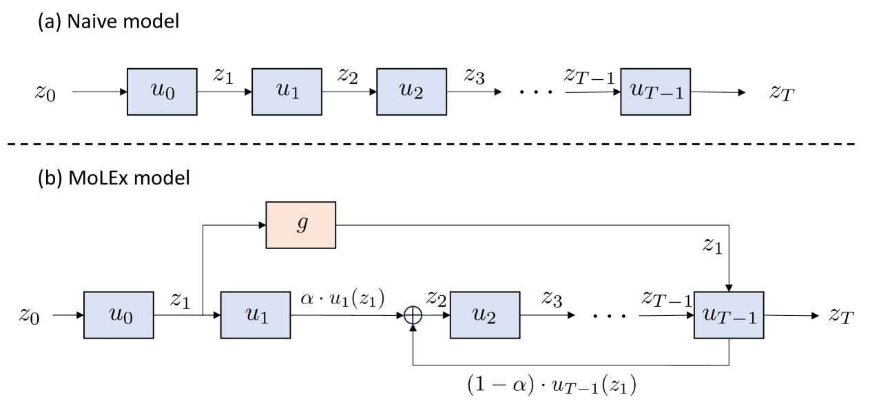
Figure 1: (a) A naive parameter efficient fine-tuning model with $T$ layers, $u_{0}$, $u_{1}$, $\cdots$, $u_{T-1}$ and input $z_{0}$. $z_{t}$, for $t=1,2,\cdots,T$ are the outputs of each layer. (b) A MoLEx model transformed from a parameter efficient fine-tuning model with $T$ layers, $u_{0}$, $u_{1}$, $\cdots$, $u_{T-1}$ and input $z_{0}$. $z_{t}$, for $t=1,2,\cdots,T$ are the outputs of each MoLEx layer. At each layer, the input to the layer is processed by a gate $g$ to select the top-1 layer expert and the outputs of the layer and the selected layer are linearly combined and weighted by $\alpha$ and $1-\alpha$ respectively. In the diagram, at layer $u_{1}$, layer $u_{T-1}$ is chosen by the gate for mixing. Then, the outputs of layer $u_{1}$ and layer $u_{T-1}$ are summed after multiplying them with $\alpha$ and $1-\alpha$ respectively.

The design of the proposed MoLEx transform in Eqn. 4 is based on the following three criteria:

(1) Preserving the useful information in the pre-trained model: In order to preserve the information in the pre-trained model, MoLEx reuses the trained layers in the pre-trained model to form a mixture of experts at each layer. Furthermore, at each layer $t$, we fix one expert to be the original layer $u_{t}$ and use the router ${\bm{g}}$ to select another expert, i.e., we use $\mathrm{Top1}$ gating function.

Let us examine an example of a 2-layer linear backbone model to illustrate how MoLEx preserves information in the pre-trained model. The backbone model $f^{(0)}$ in this case has the following form:

$${\bm{z}}_{0}={\bm{x}};\,\,{\bm{z}}_{1}={\bm{z}}_{0}+{\bm{W}}_{0}{\bm{z}}_{0};\,\,{\bm{z}}_{2}={\bm{z}}_{1}+{\bm{W}}_{1}{\bm{z}}_{1}={\bm{z}}_{0}+{\bm{W}}_{0}{\bm{z}}_{0}+{\bm{W}}_{1}({\bm{z}}_{0}+{\bm{W}}_{0}{\bm{z}}_{0}).$$

MoLEx$(f^{(0)})$ can then be rewritten as

$${\bm{z}}_{0} ={\bm{x}};{\bm{z}}_{1}={\bm{z}}_{0}+\alpha{\bm{W}}_{0}{\bm{z}}_{0}+(1-\alpha)v_{0}({\bm{z}}_{0}),$$

$${\bm{z}}_{2} ={\bm{z}}_{1}+\alpha{\bm{W}}_{1}{\bm{z}}_{1}+(1-\alpha)v_{1}({\bm{z}}_{1})$$

$$={\bm{z}}_{0}+\alpha{\bm{W}}_{0}{\bm{z}}_{0}+(1-\alpha)v_{0}({\bm{z}}_{0})+\alpha{\bm{W}}_{1}({\bm{z}}_{0}+\alpha{\bm{W}}_{0}{\bm{z}}_{0}+(1-\alpha)v_{0}({\bm{z}}_{0}))+(1-\alpha)v_{1}({\bm{z}}_{1})$$

$$=\alpha\underbrace{({\bm{z}}_{0}+{\bm{W}}_{0}{\bm{z}}_{0}+{\bm{W}}_{1}({\bm{z}}_{0}+{\bm{W}}_{0}{\bm{z}}_{0}))}_{f^{(0)}}+(1-\alpha)\underbrace{({\bm{z}}_{0}+v_{0}({\bm{z}}_{0})+v_{1}({\bm{z}}_{1}))}_{f^{(0)}_{\text{upcycled}}}+R,$$

where the remainer $R=(1-\alpha)\alpha{\bm{W}}_{1}(v_{0}({\bm{z}}_{0})-{\bm{W}}_{0}{\bm{z}}_{0})$, ${\bm{z}}_{0}={\bm{x}}$, and $v_{t}({\bm{z}}_{t})$, $t=1,2$ is defined as in Eqn. 4. As can be seen in equation above, MoLEx$(f^{(0)})$ is comprised of the pre-trained model $f^{(0)}$ and the additional upcycled part $f^{(0)}_{\text{upcycled}}$. The former component, $f^{(0)}$, allows MoLEx$(f^{(0)})$ to maintain the information in the original pre-trained model.

(2) Obtaining compositional representations: At each layer, MoLEx combines the original layer $u_{t}$ and a layer $v_{t}$ as in Eqn. 4. Since $v_{t}$ is chosen among layers in the pre-trained model $f^{(0)}$ by the $\mathrm{Top1}$ gating function, we can rewrite a layer $t$ of MoLEx$(f^{(0)})$ as

$${\bm{z}}_{t+1} ={\bm{z}}_{t}+\alpha u_{t}({\bm{z}}_{t};{\bm{\theta}}^{(0)}_{t})+(1-\alpha)u_{\tau}({\bm{z}}_{t};{\bm{\theta}}^{(0)}_{\tau}),$$ (5)

where $\tau\in\{0,1,\dots,T-1\}$. To investigate the compositional representation captured by MoLEx, we distinguish between two cases: $\tau\geq t$ and $\tau<t$.

Case 1, $\tau\geq t$ (combining with a current/later layer): We apply Taylor expansion and approximate the processing at layer $\tau$ as follows:

$$u_{\tau}({\bm{z}}_{\tau};{\bm{\theta}}^{(0)}_{\tau}) =u_{\tau}\left({\bm{z}}_{t}+\sum_{j=t}^{\tau-1}u_{j}({\bm{z}}_{j};{\bm{\theta}}^{(0)}_{j});{\bm{\theta}}^{(0)}_{\tau}\right)\approx u_{\tau}({\bm{z}}_{t};{\bm{\theta}}^{(0)}_{\tau})+u^{\prime}_{\tau}({\bm{z}}_{t};{\bm{\theta}}^{(0)}_{\tau})\sum_{j=t}^{\tau-1}u_{j}({\bm{z}}_{j};{\bm{\theta}}^{(0)}_{j}).$$

As can be seen, at layer $\tau$, $u_{\tau}$ implicitly extracts features from ${\bm{z}}_{t}$ via the term $u_{\tau}({\bm{z}}_{t};{\bm{\theta}}^{(0)}_{\tau})$. Since $\tau>t$, these features are coarse-scale/high-level features of ${\bm{z}}_{t}$ while the term $u_{t}({\bm{z}}_{t};{\bm{\theta}}^{(0)}_{t})$ in Eqn. 5 extracts the fine-scale/low-level features of ${\bm{z}}_{t}$. Layer $t$ of MoLEx$(f^{(0)})$ combines these coarse-scale/high-level and fine-scale/low-level features to attain a multi-scale compositional representation of the input data.

Case 2, $\tau<t$ (combining with a previous layer): In this case, we apply Taylor expansion to approximate $u_{\tau}({\bm{z}}_{t};{\bm{\theta}}^{(0)}_{\tau})$ as

$$u_{\tau}({\bm{z}}_{t};{\bm{\theta}}^{(0)}_{\tau}) =u_{\tau}\left({\bm{z}}_{\tau}+\sum_{j=\tau}^{t-1}u_{j}({\bm{z}}_{j};{\bm{\theta}}^{(0)}_{j});{\bm{\theta}}^{(0)}_{\tau}\right)\approx u_{\tau}({\bm{z}}_{\tau};{\bm{\theta}}^{(0)}_{\tau})+u^{\prime}_{\tau}({\bm{z}}_{\tau};{\bm{\theta}}^{(0)}_{\tau})\sum_{j=\tau}^{t-1}u_{j}({\bm{z}}_{j};{\bm{\theta}}^{(0)}_{j}).$$

Here, ${\bm{z}}_{t}={\bm{z}}_{\tau}+\sum_{j=\tau}^{t-1}u_{j}({\bm{z}}_{j};{\bm{\theta}}^{(0)}_{j})$, and $u_{\tau}$ extract finer-scale/lower-level features from ${\bm{z}}_{t}$ via the terms $u_{\tau},u_{\tau+1},\dots,u_{t-1}$ applied on ${\bm{z}}_{\tau},{\bm{z}}_{\tau+1},\dots,{\bm{z}}_{t-1}$, respectively. Layer $t$ of MoLEx$(f^{(0)})$ combines these finer-scale/lower-level features with the coarse-scale/high-level features $u_{t}({\bm{z}}_{t};{\bm{\theta}}^{(0)}_{t})$ as in Eqn. 5 to achieve a multi-scale compositional representation of the input data.

(3) Maintaining high efficiency: Even though MoLEx introduces an additional layer expert at each layer, the increase in the total number of parameters of the sparsely upcycled model due to the router ${\bm{g}}$ is negligible since MoLEx reuses layers from the pre-trained models (see Table 6). Moreover, at each layer, experts in MoLEx can be processed in parallel across different GPUs. Thus, the runtime of the MoLEx sparse upcycled model is comparable to the original model (see Table 6). Finally, from our experiments, we observe that setting $K>1$ for the $\mathrm{TopK}$ gating function in Eqn. 4 does not yield a significant improvement in the model’s performance (see Table 9). Thus, we set $K=1$ in our design of MoLEx.

Despite its simple formulation, MoLEx offers an efficient and effective approach to sparse upcycling the models. Next, we will discuss the robustness property of MoLEx as an ensemble model.

2.3 MoLEx as an Ensemble Model

In this section, we consider the simple case when $u_{j}$ is a linear layer to provide insights into the advantages of MoLEx. We start with deriving an ensemble perspective of MoLEx from the linearity of each $u_{j}$ by unrolling ${\bm{z}}_{t}$ to obtain

$$u_{j}({\bm{z}}_{t}) =u_{j}({\bm{z}}_{t-1}+\alpha u_{t-1}({\bm{z}}_{t-1})+(1-\alpha)u_{i_{t-1}}({\bm{z}}_{t-1}))$$

$$=u_{j}({\bm{z}}_{t-1})+\alpha u_{j}(u_{t-1}({\bm{z}}_{t-1}))+(1-\alpha)u_{j}(u_{i_{t-1}}({\bm{z}}_{t-1})).$$

We denote $i_{t}$ to be the layer index of the layer expert chosen by the gate at each layer $t$, i.e., to clarify, $u_{i_{t-1}}=v_{t-1}$ in Eqn. 4. Repeating this for each $j=0,\cdots,T-1$, in Eqn. 6, we write ${\bm{z}}_{t+1}$ as a linear combination of compositions of $u_{j}$ weighted by $c_{i_{0},i_{1},\cdots,i_{t}}\geq 0$, a constant that is non-zero if and only if the combination $u_{i_{t}}\circ u_{i_{t-1}}\circ\cdots\circ u_{i_{0}}$ was chosen by the gate. We can re-label each sequence of $i_{0},i_{1},\cdots,i_{t}$ to an integer $j\in\{1,2,\cdots,3^{t+1}-1\}$ and each composition of $u_{i_{t}}\circ u_{i_{t-1}}\circ\cdots\circ u_{i_{0}}$ to $f_{j}$ for $c_{i_{0},i_{1},\cdots,i_{t}}>0$ as there are at most $3^{t+1}-1$ combinations in $t$ layers of MoLEx. Then, we will have

$${\bm{z}}_{t+1} ={\bm{z}}_{t}+\alpha u_{t}({\bm{z}}_{t})+(1-\alpha)u_{i_{t}}({\bm{z}}_{t})$$ (6)

$$={\bm{z}}_{0}+\sum_{T-1\geq i_{0},i_{1},\cdots,i_{t}\geq 0}c_{i_{0},i_{1},\cdots,i_{t}}u_{i_{t}}\circ u_{i_{t-1}}\circ\cdots\circ u_{i_{0}}({\bm{x}})={\bm{x}}+\sum_{j=1}^{3^{t+1}-1}c_{j}f_{j}$$

With such an unrolling, we are able to view a linear MoLEx model as an ensemble of linear models. Next, we will show that MoLEx, as an ensemble, is more robust than a single base model in the ensemble. We begin with a formal definition of robustness.

Definition 1 ($\epsilon$-Robustness).

Consider an input ${\bm{x}}$ and a classifier model, $f:{\mathbb{R}}^{d}\rightarrow[C]$, for a $C$-way classification task where $[C]=\{1,\cdots,C\}$. If for all $\tilde{{\bm{x}}}$ within a closed ball of radius $\epsilon>0$ with center ${\bm{x}}$, i.e. $\tilde{{\bm{x}}}\in B({\bm{x}},\epsilon)=\{{\bm{x}}+\delta:\|\delta\|_{2}\leq\epsilon\}$, $f(\tilde{{\bm{x}}})=f({\bm{x}})$, then we say $f$ is $\epsilon$-robust at ${\bm{x}}$. We say that $f$ is more robust than $g$ if and only if $f$ is $\epsilon^{\prime}$-robust and $g$ is $\epsilon$-robust at $x$, with $\epsilon^{\prime}>\epsilon$.

Definition 2 (Linear MoLEx as an Ensemble Model).

From Eqn. 6, we can view a linear MoLEx model as a weighted ensemble of base functions, $f_{j}$, where each $f_{j}=u_{i_{t}}\circ u_{i_{t-1}}\circ\cdots\circ u_{i_{0}}$ is a composition of a certain permutation of the layers $u_{t}$, $t\in\{0,\cdots,T-1\}$. For simplicity, let $f_{0}=Id$, the identity function, $c_{0}=1$ and $n_{t}=3^{t+1}-1$, so that we can write ${\bm{z}}_{t+1}=\sum_{j=0}^{n_{t}}c_{j}f_{j}$ as a MoLEx model with $t+1$ layers.

We consider a set of fine-tuning sample data ${\bm{X}}$ drawn from some distribution $\chi$ with labels ${\bm{Y}}$. For the ease of understanding, we consider the output of the MoLEx model, ${\bm{z}}_{t+1}$, and a single base model with sequential layers, $f_{[0:t]}=u_{t}\circ u_{t-1}\circ\cdots u_{0}$, to be in the probability simplex, $\Delta^{C}=\{(x_{1},x_{2},\cdots,x_{C})\in{\mathbb{R}}^{C}_{\geq 0}|\sum_{j=1}^{C}x_{j}=1\}$ and refer to these as prediction models. A classifier model is then a prediction model composed with a classifier head $H({\bm{x}})=\arg\max_{i}x_{i}$ where $x_{i}$ are the elements of the vector ${\bm{x}}$. Then, our classifier model is $F({\bm{x}})=H(f({\bm{x}}))=\arg\max_{i\in[C]}f({\bm{x}})_{i}$ where $f({\bm{x}})_{i}$ is the $i$-th element in the output vector $f({\bm{x}})$.

It is not difficult to see that for an input vector ${\bm{x}}\in{\bm{X}}$ with label $y$, and a perturbed $\tilde{{\bm{x}}}\in B({\bm{x}},\epsilon)$, for a classifier $F=H(f)$ to remain $\epsilon$-robust at ${\bm{x}}$, we require that the prediction function satisfies

$$f(\tilde{{\bm{x}}})_{y}\geq f(\tilde{{\bm{x}}})_{y_{i}},\forall y_{i}\neq y$$ (7)

where $f(\tilde{{\bm{x}}})_{y_{i}}$ is the ${y_{i}}$-th element of $f(\tilde{{\bm{x}}})$. Equivalently, we state this as a lemma below.

Lemma 1 (Robustness condition for classifier model).

Consider a prediction function $f$, classifier head $H$, data point $({\bm{x}},y)\in({\bm{X}},{\bm{Y}})$ and a perturbed point $\tilde{{\bm{x}}}\in B({\bm{x}},\epsilon)$. If $F({\bm{x}})=H(f({\bm{x}}))=y$, then $F$ is $\epsilon$-Robust at ${\bm{x}}$ if and only if

$$\forall y_{i}\in[C],y_{i}\neq y,\min_{\tilde{{\bm{x}}}\in B({\bm{x}},\epsilon)}f(\tilde{{\bm{x}}})_{y}-f(\tilde{{\bm{x}}})_{y_{i}}\geq 0$$ (8)

We are now ready to state our result regarding the improved robustness of linear ensembles and we defer all proofs to the appendix in section A.

Theorem 1 (Linear ensembles are more robust).

Consider a data point $({\bm{x}},y)\in({\bm{X}},{\bm{Y}})$, $\epsilon>0$, and $M$ linear base models, $f_{j}({\bm{x}})={\bm{W}}_{j}^{\top}{\bm{x}}$ such that $\forall y_{i}$ and ${\bm{W}}_{j}$,  

$$\text{1. }\frac{1}{\epsilon}({\bm{e}}_{y}-{\bm{e}}_{y_{i}})^{\top}f_{j}({\bm{x}})\geq\|{\bm{W}}_{j}({\bm{e}}_{y}-{\bm{e}}_{y_{i}})\|_{2}$$

$$\text{2. }{\bm{W}}_{j}({\bm{e}}_{y}-{\bm{e}}_{y_{i}})\text{ are not colinear, }$$

where $e_{y}$ is the standard basis vector with $1$ at the $y$-th position and $0$ everywhere else. An ensemble classifier model, with a classification head $H$, $F_{M}=H(\sum_{j=0}^{M-1}c_{j}f_{j})$ is $\epsilon^{\prime}$-robust at ${\bm{x}}$ with $\epsilon^{\prime}>\epsilon$.

Corollary 1 (Sufficient conditions for $\epsilon$-robustness).

Consider a data point $({\bm{x}},y)\in({\bm{X}},{\bm{Y}})$, if a classifier model $F=H(f)$ with prediction function, $f({\bm{x}})={\bm{W}}^{\top}{\bm{x}}$ satisfies

$$\frac{1}{\epsilon}({\bm{e}}_{y}-{\bm{e}}_{y_{i}})^{\top}f({\bm{x}})\geq\|{\bm{W}}({\bm{e}}_{y}-{\bm{e}}_{y_{i}})\|_{2},$$

then $F$ is $\epsilon$-robust at ${\bm{x}}$.

Corollary 2 (Linear MoLEx is more robust than sequential model).

If the base models of MoLEx $f_{j}=u_{i_{t}}\circ u_{i_{t-1}}\circ...\circ u_{i_{0}}$ satisfies assumptions 1 and 2 in Theorem 1 above, then ${\bm{z}}_{t+1}=\sum_{j=0}^{n_{t}}c_{j}f_{j}$ is more robust than $f_{[0:t]}$.

Consequently, we have established the robustness of a linear MoLEx model under perturbations within a closed $\epsilon$-ball.

3 Experimental Results

In this section, we empirically validate the fine-tuning performance of MoLEx on the Natural Language Understanding (NLU) task, GLUE (Wang et al., 2018), the Natural Language Generation (NLG) benchmark, the End-to-End (E2E) dataset (Novikova et al., 2017a), and in a zero-shot evaluation on several GLUE tasks. Across all tasks and models, we apply MoLEx to LoRA on various models, including RoBERTa-base, RoBERTa-large (Liu, 2019), and GPT-2 (medium) (Radford et al., 2019). We use LoRA as our baseline for comparison. While MoLEx is compatible with any other fine-tuning method, we choose LoRA as it is one of the most popular light-weight adapters. Details on these tasks, models, metrics and implementations can be found in Appendix B. Our results are averaged over 5 runs with different seeds and conducted on a server with 8 A100 GPUs.

3.1 Natual Language Understanding

GLUE covers a wide range of domains, data types and challenge levels, making it a comprehensive benchmark for the generalizational ability of a language model. Using a pre-trained RoBERTa-base model from the HuggingFace Transformers library (Wolf et al., 2020), we fine-tune the models for all tasks using LoRA and MoLEx for comparison. To demonstrate the scalability of MoLEx to larger models, we also include RoBERTa-large and report our results in Table 1. Across all metrics, higher numbers indicate better performance.

In Table 1, we include results from prior works of other adaptation methods for reference. Details on each method can be found in the related work discussion in Section 5. As we implement MoLEx for the LoRA adaptor, we focus on that method for comparison. We observe that across almost all tasks, MoLEx outperforms the baseline LoRA on both RoBERTa-base and RoBERTa-large, demonstrating the effectiveness and scalability of our method. A key advantage of MoLEx is its enhancement of model performance without any changes to the existing method or any increase in effective parameter count. Instead, it introduces a structural modification to the model’s architecture, enabling the model to extract more information from the data, thereby leading to improved results.

Table 1: RoBERTa-base (RoB_base) and RoBERTa-large (RoB_large) fine-tuned on the popular GLUE benchmark with different adaptations methods. MoLEx (bold and shaded in gray) is our proposed method in combination with LoRA. Hence, we use LoRA as our baseline and only reproduce results for LoRA in the table. An * indicates numbers published in previous work. For all tasks, we report accuracy except for Matthew’s correlation for CoLA, Pearson correlation for STS-B, the overall (matched and mismatched) accuracy for MNLI. The average stated for models fine-tuned from the best MNLI checkpoint is the average of all tasks with results for MRPC, RTE and STS-B from the pre-trained RoBERTa checkpoint replaced by those from the MNLI checkpoint. Across almost all tasks, MoLEx surpasses the baseline LoRA on both both RoBERTa-base and RoBERTa-large, establishing its effectiveness and scalability.

Model & Method	# Trainable
	Parameters	MNLI	SST-2	MRPC	CoLA	QNLI	QQP	RTE	STS-B	Avg.
Results published in prior works for reference
RoBbase (FT)*	125.0M	87.6	94.8	90.2	63.6	92.8	91.9	78.7	91.2	86.4
RoBbase (BitFit)*	0.1M	84.7	93.7	92.7	62.0	91.8	84.0	81.5	90.8	85.2
RoBbase ($\text{Adpt}^{D}$)*	0.3M	87.1$\pm$.0	94.2$\pm$.1	88.5$\pm$1.1	60.8$\pm$.4	93.1$\pm$0.1	90.2$\pm$.0	71.5$\pm$2.7	89.7$\pm$.3	84.4
RoBbase ($\text{Adpt}^{D}$)*	0.9M	87.3$\pm$.1	94.7$\pm$.3	88.4$\pm$.1	62.6$\pm$.9	93.0$\pm$.6	90.6$\pm$.0	75.9$\pm$2.2	90.3$\pm$.1	85.4
Reproduced result from pre-trained RoBERTa checkpoint
RoBbase (LoRA)	0.3M	87.5$\pm$.2	95.0 $\pm$.1	88.7 $\pm$.3	62.8$\pm$1.0	93.2$\pm$.2	90.8 $\pm$.0	76.9$\pm$1.1	90.8$\pm$.2	85.7
RoBbase (MoLEx)	0.309M	87.7$\pm$.2	95.4 $\pm$.2	89.8$\pm$.2	64.8$\pm$.5	93.2$\pm$.2	91.0$\pm$.0	77.3$\pm$1.3	91.0$\pm$.2	86.3
RoBlarge (LoRA)	0.8M	90.7 $\pm$.1	96.3$\pm$.2	90.9$\pm$.4	67.8$\pm$1.7	94.8$\pm$.3	91.5$\pm$.1	86.5$\pm$.9	91.9$\pm$.1	88.8
RoBlarge (MoLEx)	0.8M	90.9 $\pm$.1	96.4$\pm$.2	91.4$\pm$.7	68.2$\pm$.2	94.8$\pm$.0	91.6$\pm$.1	87.1$\pm$.9	92.0$\pm$.2	89.1
Reproduced result from fine-tuned MNLI checkpoint
RoBbase (LoRA)	0.3M	-	-	89.7 $\pm$.6	-	-	-	86.8 $\pm$.2	91.3 $\pm$.1	87.1
RoBbase (MoLEx)	0.3M	-	-	91.1 $\pm$.6	-	-	-	86.8 $\pm$.2	91.3 $\pm$.0	87.6

3.2 Natual Language Generation

To further illustrate the versatility of our method on different language tasks, we evaluate MoLEx on the standard E2E NLG Challenge dataset introduced by (Novikova et al., 2017b) for training end-to-end, data-driven NLG systems. We fine-tune GPT-2 medium on E2E, following the set up of Li & Liang (2021), and report our results in Table 2. For all metrics, higher is better.

Similar to Table 1, in Table 2, we also include results from previous works. This is for reference, and we describe those methods in more detail in Section 5. Compared with the baseline LoRA method, MoLEx outperforms significantly on 3 metrics with a remarkable increase on BLEU by 0.7. We further note that the standard deviations for MoLEx is generally lower than LoRA. This aligns with our analysis of MoLEx as an ensemble model, which is expected to have lower variance (Ganaie et al., 2022; Gupta et al., 2022), and improves the reliability of the model in language generation.

Table 2: GPT2 medium (M) fine-tuned on the standard E2E NLG Challenge benchmark. We reproduce the LoRA baseline and compare it to our proposed method MoLEx (bold and shaded in gray) using the usual BLEU, NIST, MET, ROUGE-L and CIDEr metrics, where higher numbers indicate better performance. An * indicates numbers published in previous work and we include them in the table for reference. MoLEx significantly outperforms the baseline LoRA on 3 metrics with lower standard deviations, verifying its advantage.

Model & Method	# Trainable	E2E NLG Challenge
	Parameters	BLEU	NIST	MET	ROUGE-L	CIDEr
Results published in prior works for reference
GPT-2 M (FT)*	354.92M	68.2	8.62	46.2	71.0	2.47
GPT-2 M (AdapterL)*	0.37M	66.3	8.41	45.0	69.8	2.40
GPT-2 M (AdapterL)*	11.09M	68.9	8.71	46.1	71.3	2.47
GPT-2 M (AdapterH)*	11.09M	67.3$\pm$.6	8.50$\pm$.07	46.0$\pm$.2	70.7$\pm$.2	2.44$\pm$.01
GPT-2 M (FTTop2)*	25.19M	68.1	8.59	46.0	70.8	2.41
GPT-2 M (PreLayer)*	0.35M	69.7	8.81	46.1	71.4	2.49
Results reproduced for comparison
GPT-2 M (LoRA)	0.35M	70.0 $\pm$.5	8.77$\pm$.05	46.8 $\pm$.2	71.6$\pm$.3	2.52$\pm$.01
GPT-2 M (MoLEx)	0.359M	70.7 $\pm$.4	8.87$\pm$.03	46.5$\pm$.09	71.8$\pm$.1	2.52$\pm$.01

3.3 Zero-shot transfer learning

We assess the ability of LoRA and MoLEx to transfer knowledge across relatively similar tasks in a zero-shot transfer learning setup on GLUE using RoBERTa-base. In Table 3, we present an evaluation of MoLEx in comparison with the baseline LoRA method when fine-tuned on one task and evaluated on another without any additional training. These pairs of tasks are QQP and MRPC (both test for semantic similarity), QQP and QNLI (both involve parsing questions), and QNLI and RTE (both are inference tasks). For all tasks, as they are binary classifications, when necessary, we reverse the class labels on the classifier head to obtain the best accuracy. In doing so, we are consistent across both models.

Table 3 suggests that MoLEx can generalize better to new data distributions compared to LoRA as across all evaluations, mixing layers consistently leads to significant improvements in zero-shot performance on new tasks. These results illustrate the ability of MoLEx to improve the model’s transferability between different classification tasks, further validating our approach.

Table 3: Zero-shot evaluation of RoBERTa-base on several GLUE tasks, QNLI, RTE, MRPC, and QQP when fine-tuned with LoRA and our MoLEx (bold and shaded in gray) on different tasks. As we only consider pairs of similar tasks for meaningful comparison, we report the relevant ones and mark the others with a dash. For all pairs of tasks considered, MoLEx outperforms the baseline LoRA by a large margin.

Fine-tune on	Evaluate on
	QNLI		RTE		MRPC		QQP
	LoRA	MoLEx	LoRA	MoLEx	LoRA	MoLEx	LoRA	MoLEx
QNLI			56.7$\pm$1.1	59.9$\pm$1.3	-	-	63.2$\pm$.0	65.7$\pm$.0
RTE	56.1$\pm$.2	58.5$\pm$.2			-	-	-	-
MRPC	-	-	-	-			65.7$\pm$.0	67.9$\pm$.0
QQP	50.5$\pm$.2	56.2$\pm$.2	-	-	67.2$\pm$.4	69.9$\pm$.7

4 Empirical Analysis

We conduct probing on MoLEx, additional experiments on robustness and efficiency, and an ablation study to provide more understandings of MoLEx.

4.1 Probing Tasks

Language models, such as RoBERTa (Liu, 2019), attain impressive results on a multitude of NLP tasks that range in complexity, even with fine-tuning on a small subset of parameters (Zaken et al., 2021; Rücklé et al., 2021; Xu et al., 2023; Pfeiffer et al., 2021; Lin et al., 2020; Houlsby et al., 2019; Li & Liang, 2021). This suggests that the pre-trained base model already captures important linguistic properties of sentences that are capitalized upon during training on different tasks. At this junction, MoLEx with its unique feature of layer mixing can be leveraged to shed light on how the linguistic properties captured in the pre-trained base model can be combined for different downstream finetuning tasks.

We analyze the semantic nature captured by the representations in each layer of RoBERTa using the probing tasks proposed in (Conneau et al., 2018) and following the setup in (Jawahar et al., 2019). For each probe, an auxiliary classification task is set up where the representations are used as features to predict certain linguistic properties of interest. The better the performance of the classifier, the more likely that the layer’s hidden embedding encodes for that particular property. These results are presented in Table 4. By piecing together the type of information mixed in each layer of MoLEx, we enhance our understanding of the language processing occurring in a RoBERTa model during fine-tuning and improve the interpretability of neural networks in NLP (Belinkov & Glass, 2019). We will focus on CoLA (single-sentence), STS-B (similarity and paraphrase) and RTE (inference) as representative tasks and examine the layers chosen for mixing to understand the key features that enable the model to excel on each type of task.

The 10 probes can be grouped into 3 different categories, surface, syntactic, and semantic information tasks. Briefly, sentence length (SentLen) and word content (WC) fall under surface level information; the bigram shift (BShift), tree depth (TreeD) and top constituent (TopConst) tasks represent syntactic information; and the final 5 tasks, Tense, Subject Number (SubjNum), Object Number (ObjNum), semantic odd man out (SOMO) and coordination inversion (CoordInv) are considered semantic information. Detailed explanations on each task and their implementations can be found in the Appendix C. We provide our probing results for RoBERTa in Table 4 and discuss these results in detail in Appendix C.4.

Table 4: Probing task performance (accuracy of a simple MLP classifier) for each layer of RoBERTa-base. Bolded numbers are the top 2 values within each task.

Layer	SentLen	WC	TreeD	TopConst	BShift	Tense	SubjNum	ObjNum	SOMO	CoordInv
	(Surface)	(Surface)	(Syntactic)	(Syntactic)	(Syntactic)	(Semantic)	(Semantic)	(Semantic)	(Semantic)	(Semantic)
0	91.48	4.10	32.00	48.93	50.00	82.27	77.56	73.81	49.87	57.47
1	87.99	0.61	29.75	35.10	54.32	79.74	74.05	71.83	49.87	50.00
2	87.03	0.33	29.06	29.32	64.99	82.06	78.51	73.49	49.88	50.00
3	85.78	0.16	29.30	29.26	73.29	82.29	76.14	74.69	50.07	50.00
4	85.32	2.40	31.06	54.12	77.95	84.37	77.33	73.67	59.21	57.69
5	84.15	1.97	31.83	57.57	81.82	85.35	80.80	78.53	62.74	60.05
6	82.17	2.91	31.81	59.90	82.41	85.61	81.22	81.48	63.67	61.97
7	79.75	0.68	28.99	48.44	82.34	84.79	80.28	80.26	64.94	57.88
8	80.49	1.09	30.73	52.24	83.56	86.81	81.65	80.92	65.00	65.07
9	77.75	1.06	29.83	49.96	83.10	86.19	81.63	79.14	64.52	66.28
10	66.65	1.15	26.97	43.68	82.59	85.25	80.91	75.95	61.78	61.92
11	73.69	18.25	30.56	60.26	85.25	87.55	82.92	79.51	63.52	66.62

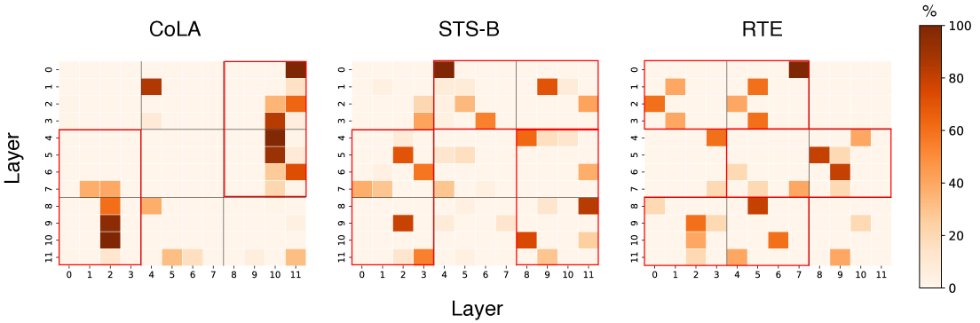
Figure 2: Heat maps to visualize the percentage of time each layer expert is chosen at every layer of MoLEx when fine-tuning RoBERTa-base on GLUE tasks, CoLA, STS-B and RTE. As one expert is fixed to be the original layer, the x-axis corresponds to the sequential layer while the y-axis corresponds to the layer experts.

Key Linguistic Features for Task Performance. In Figure 2, from left to right, there is an increasing degree of mixing between all layers that correlates with the increasing complexity of each task. In particular, since RTE is an inference task that requires a deeper understanding of the input sentences, it is not surprising that MoLEx mixes nearly all layers to a greater extent for this task than for both CoLA and STS-B. We discuss the probing for each task below.

CoLA evaluates grammatical acceptability and, as shown in Figure 2, focuses on later layers, which capture semantic information like tense and word placement—key for grammatical correctness. STS-B measures sentence similarity, with Figure 2 showing significant mixing in later layers for rich contextual data and earlier layers for surface features like sentence length, reflecting task-specific needs. RTE, a binary entailment classification task, emphasizes middle layers, aligning with the syntactic structure required for logical understanding. These observations suggest the model adapts its layer usage to the linguistic demands of each task.

4.2 Robustness

Table 5: Robustness (in accuracy) of RoBERTa-base on GLUE tasks, QNLI, and SST2 when fine-tuned with LoRA and MoLEx. Random noise is added to the input during evaluation. MoLEx is more robust than the LoRA baseline.

Method	QNLI	SST-2
	(with added noise)
LoRA	63.1 $\pm$.2	69.3$\pm$.1
MoLEx	64.0$\pm$.2	70.9$\pm$.2

Though the models used in our experiments are non-linear, we expect that the theoretical robustness properties still hold and can be extended to practical situations. To verify this, we perform a simple experiment using MoLEx and LoRA in a RoBERTa-base model trained on 2 GLUE tasks as described in Section 3 and present the results in Table 5. For the tasks presented, we add random noise into the input data for evaluation and find that MoLEx is indeed more robust to noise than the baseline LoRA model as it achieves a higher accuracy on both tasks. We do not report the results for the other tasks, as adding noise causes both models to have an accuracy equivalent to random guessing.

4.3 Efficiency Analysis & Ablation Study

We provide the run time per sample, memory, and number of parameters of MoLEx compared to the baseline LoRA in Table 6 and a more detailed analysis in Appendix E.3. There is only a marginal increase in compute time due to the additional gating function. Also, in Table 9, Appendix D, we conduct 3 GLUE tasks, CoLA, QQP, and SST-2 when using Top1 and Top2 routing. We observe that Top1 yields better results. Thus, we use a Top1 routing for MoLEx.

Table 6: Run time per sample, memory, and number of parameters for baseline LoRA and our MoLEx in RoBERTa-base during inference time.

Method	Sec/Sample	Memory	Parameters
	(Inference)	(Inference)
LoRA (baseline)	0.00345	1890MB	0.3M
MoLEx	0.00357	1892MB	0.3M

5 Related Work

Parameter-Efficient Fine-Tuning (PEFT). The simplest solution of PEFT is to only update a small subset of weights (partial fine-tuning) (Li & Liang, 2021). For comparison, we include results from a previous work that kept all layers except the last 2 frozen on GPT-2 in Table 2 (FT^Top2) (Li & Liang, 2021). Other methods that fine-tune a selected subset of parameters include BiTFiT (Zaken et al., 2021), where only the bias vectors are updated, and its extension using Neural Architecture Search (Lawton et al., 2023). A separate approach is to introduce extra trainable parameters into the model for adaptation. These include soft prompt-based tuning where trainable word embeddings are inserted among the input tokens (Hambardzumyan et al., 2021; Lester et al., 2021; Liu et al., 2023; Zhang et al., 2023) or prepended to the hidden states of the multi-head attention layer (prefix-tuning) (Li & Liang, 2021). Another method is prefix-layer tuning (PreLayer) that learns new activations after every Transformer layer. Qi et al. (2022) suggests only training the gain and bias term of the LayerNorm in the model. In addition, adapter tuning (Houlsby et al., 2019) involves inserting adapter layers into a transformer layer. This design is denoted as Adapter^H in Table 2. More efficient methods have also been proposed by (Lin et al., 2020; Pfeiffer et al., 2021) to reduce the number of adapter layers (Adapter^L) and by (Rücklé et al., 2021) to drop adapter layers (Adapter^D). Recently, neural functional networks have emerged as a promising alternative to PEFT (Zhou et al., 2023a; b; Mitchell et al., 2022; Vo et al., 2024; Sinitsin et al., 2020; Navon et al., 2023; Tran et al., 2025a; b).

Neural Network Intepretability. The study of how models learn language structure during training is gaining interest. (Belinkov & Glass, 2019). Specifically, there is interest in deciphering the type of linguistic knowledge encoded in sentence and word embeddings (Dalvi et al., 2017; Belinkov et al., 2017; 2018; Sennrich, 2017). Many studies focus on uncovering the structural properties of language captured by BERT (Devlin et al., 2018) mainly through various linguistic probes on the representations produced by the model (Devlin et al., 2018; Liu et al., 2019; Tenney et al., 2019; Hewitt & Manning, 2019; Conneau et al., 2018) and well-designed evaluation protocols and stimuli (Goldberg, 2019; Marvin, 2018; Gulordava, 2018; Linzen et al., 2016). There is also a general consensus that language models learn linguistic information hierarchically (Peters et al., 2018).

6 Concluding Remarks

In this paper, we introduce a Mixture of Layer Experts (MoLEx), a novel approach that leverages layers as experts to facilitate the exchange of linguistic information and improve a model’s fine-tuning and transfer knowledge ability. Orthogonal to current PEFT methods, we do not add in or modify any internal components in the model. Instead, we propose a structural change to the architecture of the model that can be effortlessly integrated with any PEFT method while maintaining the same number of effective parameters. We theoretically justify the robustness of MoLEx in a simplified model and provide empirical evidence for it. Our experiments demonstrate that MoLEx significantly improves performance across a range of downstream tasks, including the GLUE benchmark and the E2E Challenge, while incurring minimal additional computational overhead and scales well with model size. Additionally, MoLEx’s unique architecture also enhances model interpretability. A limitation of our work is that our robustness guarantee is only for deep linear models. Extending this result to the case of deep nonlinear models, as well as exploring layer mixing across different models, is an interesting direction to pursue. We leave these exciting research ideas as future work.

Acknowledgments

This research / project is supported by the National Research Foundation Singapore under the AI Singapore Programme (AISG Award No: AISG2-TC-2023-012-SGIL). This research / project is supported by the Ministry of Education, Singapore, under the Academic Research Fund Tier 1 (FY2023) (A-8002040-00-00, A-8002039-00-00). This research / project is also supported by the NUS Presidential Young Professorship Award (A-0009807-01-00) and the NUS Artificial Intelligence Institute–Seed Funding (A-8003062-00-00) . Reproducibility Statement. Source code for our experiments are provided in the supplementary material. We provide the full details of our experimental setup – including datasets, model specification, train regime, and evaluation protocol – for all experiments Section 3 and Appendix B. All datasets are publicly available.

Ethics Statement. Given the nature of the work, we do not foresee any negative societal and ethical impacts of our work.

Supplement to “MoLEx: Mixture of Layer Experts for Finetuning with Sparse Upcycling”

1Table of Contents

  

Appendix A Proofs

A.1 Proof of Theorem 1

We restate the theorem below for convenience.

Theorem 1 (Linear ensembles are more robust than base models).

For a data point $({\bm{x}},y)\in({\bm{X}},{\bm{Y}})$, and $M$ linear base models, $f_{j}({\bm{x}})={\bm{W}}_{j}^{\top}{\bm{x}}$ such that $\forall y_{i}$ and ${\bm{W}}_{j}$,

1. $\frac{1}{\epsilon}({\bm{e}}_{y}-{\bm{e}}_{y_{i}})^{\top}f_{j}({\bm{x}})\geq\|{\bm{W}}_{j}({\bm{e}}_{y}-{\bm{e}}_{y_{i}})\|_{2}$

2. ${\bm{W}}_{j}({\bm{e}}_{y}-{\bm{e}}_{y_{i}})$ are not colinear,

an ensemble classifier model, with a classification head $H$, $F_{M}=H(\sum_{j=0}^{M-1}c_{j}f_{j})$ is $\epsilon^{\prime}$-robust at ${\bm{x}}$ with $\epsilon^{\prime}>\epsilon$.

Proof.

For a linear ensemble classifier, $F_{M}$ to be robust, from Lemma 1, we require that $\forall y_{i}\in[C],y_{i}\neq y,\min_{\tilde{{\bm{x}}}\in B({\bm{x}},\epsilon)}\sum_{j=0}^{M-1}c_{j}(f_{j}(\tilde{{\bm{x}}})_{y}-f_{j}(\tilde{{\bm{x}}})_{y_{i}})\geq 0$. Expanding this, with ${\bm{e}}_{y}$ being the standard basis vector with $1$ in the $y$-th position,

$$\min_{\tilde{{\bm{x}}}\in B({\bm{x}},\epsilon)}\sum_{j=0}^{M-1}c_{j}(f_{j}(\tilde{{\bm{x}}})_{y}-f_{j}(\tilde{{\bm{x}}})_{y_{i}})$$

$$=\min_{\tilde{{\bm{x}}}\in B({\bm{x}},\epsilon)}\sum_{j=0}^{M-1}c_{j}({\bm{e}}_{y}-{\bm{e}}_{y_{i}})^{\top}f_{j}(\tilde{{\bm{x}}})$$

$$=\min_{\tilde{{\bm{x}}}\in B({\bm{x}},\epsilon)}\sum_{j=0}^{M-1}c_{j}({\bm{e}}_{y}-{\bm{e}}_{y_{i}})^{\top}({\bm{W}}_{j}^{\top}{\bm{x}}+{\bm{W}}_{j}^{\top}(\tilde{{\bm{x}}}-{\bm{x}}))$$

$$=\sum_{j=0}^{M-1}c_{j}({\bm{e}}_{y}-{\bm{e}}_{y_{i}})^{\top}f_{j}({\bm{x}})+\min_{\tilde{{\bm{x}}}\in B({\bm{x}},\epsilon)}({\bm{e}}_{y}-{\bm{e}}_{y_{i}})^{\top}(\sum_{j=0}^{M-1}c_{j}{\bm{W}}_{j}^{\top})(\tilde{{\bm{x}}}-{\bm{x}})$$

$$=\sum_{j=0}^{M-1}c_{j}({\bm{e}}_{y}-{\bm{e}}_{y_{i}})^{\top}f_{j}({\bm{x}})+\min_{\tilde{{\bm{x}}}\in B({\bm{x}},\epsilon)}(\bar{{\bm{W}}}({\bm{e}}_{y}-{\bm{e}}_{y_{i}}))^{\top}(\tilde{{\bm{x}}}-{\bm{x}})$$

$$\geq\sum_{j=0}^{M-1}c_{j}({\bm{e}}_{y}-{\bm{e}}_{y_{i}})^{\top}f_{j}({\bm{x}})-\epsilon\|\bar{{\bm{W}}}({\bm{e}}_{y}-{\bm{e}}_{y_{i}})\|_{2}$$

where the last inequality holds by the Cauchy-Schwartz inequality and we denote $\bar{{\bm{W}}}^{\top}:=(\sum_{j=0}^{M-1}c_{j}f_{j})=\sum_{j=0}^{M-1}c_{j}{\bm{W}}_{j}^{\top}$ to represent our ensemble function. Hence, if the following holds,

$$\sum_{j=0}^{M-1}c_{j}({\bm{e}}_{y}-{\bm{e}}_{y_{i}})^{\top}f_{j}({\bm{x}})-\epsilon\|\bar{{\bm{W}}}({\bm{e}}_{y}-{\bm{e}}_{y_{i}})\|_{2}\geq 0\iff\frac{1}{\epsilon}\sum_{j=0}^{M-1}c_{j}({\bm{e}}_{y}-{\bm{e}}_{y_{i}})^{\top}f_{j}({\bm{x}})\geq\|\bar{{\bm{W}}}({\bm{e}}_{y}-{\bm{e}}_{y_{i}})\|_{2},$$

then $F_{M}$ is robust. Since, in our assumption 2, $\forall y_{i}$ and ${\bm{W}}_{j}$, ${\bm{W}}_{j}({\bm{e}}_{y}-{\bm{e}}_{y_{i}})$ are not colinear, from triangle inequality and assumption 1, we have

$$\|\bar{{\bm{W}}}({\bm{e}}_{y}-{\bm{e}}_{y_{i}})\|_{2}=\|\sum_{j=0}^{M-1}c_{j}{\bm{W}}_{j}({\bm{e}}_{y}-{\bm{e}}_{y_{i}})\|_{2} <\sum_{j=0}^{M-1}c_{j}\|{\bm{W}}_{j}({\bm{e}}_{y}-{\bm{e}}_{y_{i}})\|_{2}$$

$$\leq\frac{1}{\epsilon}\sum_{j=0}^{M-1}c_{j}({\bm{e}}_{y}-{\bm{e}}_{y_{i}})^{\top}f_{j}({\bm{x}})$$

As the inequality holds strictly, we can always find an $\epsilon^{\prime}>\epsilon$ such that the inequality still holds. Hence, $F_{M}$ is $\epsilon^{\prime}$-robust. ∎

A.2 Proof of Corollary 1

We restate the corollary below for convenience.

Corollary 1 (Sufficient conditions for $\epsilon$-robustness).

For a data point $({\bm{x}},y)\in({\bm{X}},{\bm{Y}})$, if a classifier model $F=H(f)$ with prediction function, $f({\bm{x}})={\bm{W}}^{\top}{\bm{x}}$ satisfies $\frac{1}{\epsilon}({\bm{e}}_{y}-{\bm{e}}_{y_{i}})^{\top}f({\bm{x}})\geq\|{\bm{W}}({\bm{e}}_{y}-{\bm{e}}_{y_{i}})\|_{2}$, then $F$ is $\epsilon$-robust at ${\bm{x}}$.

Proof.

This result follows directly from the proof of Theorem 1, with $M=1$. ∎

A.3 Proof of Corollary 2

We restate the corollary below for convenience.

Corollary 2 (Linear MoLEx is more robust than sequential model).

If the base models of MoLEx $f_{j}=u_{i_{t}}\circ u_{i_{t-1}}\circ...\circ u_{i_{0}}$ satisfies assumptions 1 and 2 in Theorem 1 above, then ${\bm{z}}_{t+1}=\sum_{j=0}^{n_{t}}c_{j}f_{j}$ is more robust than $f_{[0:t]}$.

Proof.

In each layer $t$ of MoLEx, as one layer expert is always fixed to be the original pre-trained layer $u_{t}$, the sequential model, $f_{[0:t]}$ will always be one of the base models. Then, by Corollary 1 and assumption 1, $f_{[0:t]}$ is $\epsilon$-robust. The rest of the corollary follows as a consequence of Theorem 1 as ${\bm{z}}_{t+1}$ will be $\epsilon^{\prime}$-robust with $\epsilon^{\prime}>\epsilon$. ∎

Appendix B Additional Experimental Details

B.1 Natural Language Understanding: GLUE

Tasks: CoLA (Warstadt et al., 2019) consists of sequences of words taken from books and journal articles on linguistic theory with labels to determine if they are grammatically acceptable or not. SST-2 (Socher et al., 2013) comprises of movie reviews and the task is to predict their sentiments as positive or negative. MRPC (Dolan & Brockett, 2005) is a corpus of pairs of sentences pulled from online news sources and annotated by humans whether they are semantically equivalent. The QQP dataset was collated from the community question-answering website Quora. It contains question pairs and simlar to MRPC, the goal is to determine if they are labelled to be semantically equivalent. STS-B (Cer et al., 2017) is another sentence pair similarity task extracted from news headlines, video and image captions, and natural language inference data. However, it differs from the previous tasks in not using binary labels and instead each examples is accompanied by a similarity score from 1 to 5. MNLI (Williams et al., 2018) uses pairs of premise and hypothesis sentences that have been collected from ten different sources, including transcribed speech, fiction, and government reports. The objective is to predict whether the premise entails the hypothesis (entailment), contradicts the hypothesis (contradiction), or neither (neutral). QNLI (Rajpurkar et al., 2018) is a task to determine if the context sentence in a question-sentence pair contains the answer to the question. The sentences were taken from paragraphs in Wikipedia and the questions were annotated by humans. Lastly, we have RTE (Dagan et al., 2006; Bar-Haim et al., 2006; Giampiccolo et al., 2007; Bentivogli et al., 2009), a compilation of datasets from a series of annual textual entailment challenges. Similar to MNLI, the objective is to determine if the sentence pairs contain an entailment or not. The classes for contradiction and neutral as in MNLI are collapsed into a single non-entailment class.

Metrics: All tasks in GLUE are classification tasks, except for STS-B which is a regression task. Therefore, the metric reported for STS-B is the Pearson correlation coefficient as is standard practise. We report the overall accuracy for MNLI which includes both matched and mismatched data. These correspond to evaluations on pairs of sentences within the same domain or cross-domain respectively. On CoLA, we use the Matthews correlation coefficient (Matthews, 1975) for evaluation due to the unbalanced binary classification data. This metric ranges from -1 to 1, with 0 indicating random guessing. For all other tasks, we present their accuracy for evaluation. Across all metrics, a higher number reflects stronger performance.

Model: We use the pre-trained RoBERTa-base and RoBERTa-large model (Liu, 2019) from the HuggingFace Transformers library (Wolf et al., 2020) for evaluation on the GLUE task. RoBERTa is an optimized version of the original pre-training recipe proposed in BERT (Devlin et al., 2018). RoBERTa-base has 125M parameters with 12 layers, 12 attention heads and 768 hidden dimensions while RoBERTa-large has 355M parameters with 24 layers, 16 attention heads and 1024 hidden dimensions.

Implementation details: We follow the same fine-tuning set up as in the original LoRA (Hu et al., 2021) paper for all GLUE experiments using the their publicly available code https://github.com/microsoft/LoRA. We use the same setting for fine-tuning on the pre-trained model and from an MNLI checkpoint. For each task, we also optimize the hyperparameters of the gate used in deciding the layer experts to be used for mixing. These settings can be found in Table 7 and for all gates, we use the same optimizer, AdamW (Loshchilov, 2017), as the LoRA parameters with a learning rate of 0.1 and weight decay of 0.01. We report the mean and standard deviation over 5 random seeds for all results and the result for each run is taken from the best epoch.

While we employ batch routing in the mixture of layers, each token will have a different choice of layer to be routed to as every token is processed by the gate. In deciding the overall batch’s decision, we use 2 different aggregates. The first is a majority-takes-all scheme where we route the batch to the layer which majority of tokens have chosen. The second is to use the maximum over the mean probability vector of all the tokens choices. These are referred to as Mode and Mean respectively under Batch Agg in the table. For gate types with suffix ”Sig” we use a sigmoid activation before taking TopK values and the default is a softmax activation. For almost all gates, if they do not have an ”Indv Gate”, this means that we use the same gate for all layers to decide the mixing layers. On RTE and STS-B, we use individual gates, which means that each layer has its own linear gating function and mixing weights instead of sharing one between all the layers. For all tasks, if the mixing weights are fixed, we use $\alpha=0.95$ as defined in Eqn. 4.

Table 7: Hyperparameter settings for LoRA and MoLEx on each GLUE task when fine-tuning RoBERTa-base and RoBERTa-large.

Method	Dataset	MNLI	SST-2	MRPC	CoLA	QNLI	QQP	RTE	STS-B
	Optimizer	AdamW
	Warmup Ratio	0.06
	LR Schedule	Linear
RoBERTa-base LoRA	Batch Size	16	16	16	32	32	16	32	16
	# Epochs	30	60	30	80	25	25	80	40
	Learning Rate	5E-04	5E-04	4E-04	4E-04	4E-04	5E-04	5E-04	4E-04
	LoRA Config.	$r_{q}=r_{v}=8$
	LoRA $\alpha$	8
	Max Seq. Len.	512
RoBERTa-base MoLEx gate	Gate Type	Cos-Sig	Cos	Linear	Linear	Cos	Cos-Sig	Linear	Linear
	Projection Dim	416	128	-	-	96	384	-	-
	Indv Gate	$\times$	$\times$	$\times$	$\times$	$\times$	$\times$	$\checkmark$	$\checkmark$
	Batch Agg	Mode	Mode	Mode	Mode	Mean	Mode	Mean	Mean
	Mixing Weights	Learn	Learn	Learn	Fix	Learn	Learn	Fix	Fix
	Load Balance	0.005	0.01	0.0	0.01	0.001	0.001	0.001	0.006
RoBERTa-large LoRA	Batch Size	4	4	4	4	4	4	8	8
	# Epochs	10	10	20	20	10	20	20	30
	Learning Rate	3E-04	4E-04	3E-04	2E-04	2E-04	3E-04	4E-04	2E-04
	LoRA Config.	$r_{q}=r_{v}=8$
	LoRA $\alpha$	16
	Max Seq. Len.	128	128	512	128	512	512	512	512
RoBERTa-large MoLEx gate	Gate Type	Cos	Cos	Linear	Linear	Cos	Cos-Sig	Linear	Linear
	Projection Dim	416	64	-	-	256	384	-	-
	Indv Gate	$\times$	$\times$	$\checkmark$	$\times$	$\times$	$\times$	$\checkmark$	$\checkmark$
	Batch Agg	Mode	Mode	Mode	Mode	Mean	Mode	Mode	Mode
	Mixing Weights	Fix	Fix	Fix	Fix	Fix	Learn	Fix	Fix
	Load Balance	0.0001	0.0	0.0001	0.01	0.001	0.001	0.0	0.0

B.2 Natural Language Generation: E2E

Dataset: The E2E NLG dataset approximately consists of more than 50,000 examples from the restaurant domain and there is a 76.5-8.5-15 split of the dataset into a training, validation and test set respectively. The E2E dataset is commonly used for the evaluation of data-to-text tasks and brings new challenges such as open vocabulary, complex syntactic structures and diverse discourse phenomena. Every data input consists of a meaning representation (MR) that includes a sequence of attribute-value pairs and a corresponding target, a natural language (NL) reference text.

Metrics: We report the same metrics as in (Novikova et al., 2017b), namely BLEU (Papineni et al., 2002), NIST (Doddington, 2002), METEOR (Lavie & Agarwal, 2007), ROUGE-L (Lin, 2004) and CIDEr (Vedantam et al., 2015). BLEU is a method to evaluate the quality of automated machine translations that scales the geometric mean of the precision scores of the n-grams in a generated text by an exponential brevity penalty factor. Similarly, NIST is based on BLEU with some slight changes. NIST uses weighted precision scores of the n-grams determined by how informative each of them are, instead of an equal weighting as in BLEU, and loosens the brevity penalty for small variations. METEOR evaluates the quality of the generated text at a segment level. It constructs a word alignment between strings and scores them using a parameterized harmonic mean of their unigram precision and recall. ROGUE-L is a metric that naturally captures sentence level structures by only awarding scores to in-sequence co-occurrences in the predicted and reference text. Lastly, CIDEr is a measure for how well the generated text matches the consensus of a set of reference image descriptors. It scores the frequency of n-grams in the generated text that occurs in the reference sentences and discounts n-grams that appear commonly across all images in the dataset.

Model: We use the pre-trained GPT-2 medium (Radford et al., 2019) from the HuggingFace Transformers library (Wolf et al., 2020) for evaluation on the E2E dataset. GPT-2 medium contains 355M parameters with 24 layers, 16 attention heads and 1,024 hidden dimensions.

Implementation details: We follow the same fine-tuning setup as in Li & Liang (2021) and LoRA (Hu et al., 2021) using their publicly available code https://github.com/microsoft/LoRA. We also optimize the hyperparameters of the gate used in deciding the layer experts to be used for mixing. These settings can be found in Table 8 and we use the same optimizer, AdamW (Loshchilov, 2017), as the LoRA parameters with a learning rate of 0.1 and weight decay of 0.01. We report the mean and standard deviation over 5 random seeds for all results and the result for each run is taken from the best epoch.

While we employ batch routing in MoLEx, each token will have a different choice of layer to be routed to as every token is processed by the gate. In deciding the overall batch’s decision for GPT-2, we use a majority-takes-all scheme where we route the batch to the layer which majority of tokens have chosen (Mode). We use a linear gating function with a softmax activation and only implement MoLEx in the first 12 layers of the model. The mixing weights are fixed and we use a value of $\alpha=0.95$ as defined in Eqn. 4. All layers share the same gate for routing.

Table 8: Hyperparameter settings for LoRA and MoLEx on the E2E NLG task when fine-tuning GPT-2 medium (M).

GPT-2 M LoRA	Dataset	E2E
Training
	Optimizer	AdamW
	Weight Decay	0.01
	Dropout Prob	0.1
	Batch Size	8
	# Epoch	5
	Warmup Steps	500
	Learning Rate Schedule	Linear
	Label Smooth	0.1
	Learning Rate	0.0002
	Adaptation	$r_{q}=r_{v}=4$
	LoRA $\alpha$	32
GPT-2 M MoLEx gate	Gate Type	Linear
	Layers with MoLEx	0 to 11 (inclusive)
	Indv Gate	$\times$
	Batch Agg	Mode
	Mixing Weights	Fixed
	Load Balance	0.01
Inference
	Beam Size	10
	Length Penalty	0.9
	No Repeat Ngram Size	4

Appendix C Additional Empirical Analysis Details

C.1 Probing Tasks

Probing (or diagonostic) tasks (Adi et al., 2016; Hupkes et al., 2018; Conneau et al., 2018) aid us in the discovery of linguistic features potentially encoded in a deep learning model. Specifically, in the hidden representations of the input in each layer. In order to understand these representations using a probe, an auxiliary classification task is set up where the representations are used as features to predict certain linguistic properties of interest. The better the performance of the classifier, the more likely that the layer’s hidden embedding encodes for that particular property. Using the 10 probing tasks developed by (Conneau et al., 2018) and inspired by (Jawahar et al., 2019), who had done a similar analysis on BERT, we evaluate each layer of RoBERTa and present the results in Table 4.

In each tasks’s dataset, there are 100K training sentences and 10K-sentence validation and test sets. All sets are equally balance among the target classes. These datasets were constructed by (Conneau et al., 2018) from the Toronto Book Corpus (Zhu, 2015; Paperno et al., 2016).

Surface Information: SentLen is a task to predict the length of a sentence, which is considered to be the number of words in the sentence. It is converted into a 6-way classification task by grouping sentence lengths into 6 equal-width bins. WC is a classification task with 1000 classes. Each class is a word and each input is a sentence that contains one and only one of the words within those classes. The task is to predict which word is contained within the input sentence.

Syntactic Information: BShift is a binary classification task where half the dataset has sentences intact and another half has sentences with 2 random adjacent words inverted. The goal is to predict if the sentence has a legal word order or if it has been inverted. TreeD assesses whether the hierarchical structure of sentences can be inferred from the hidden layer’s embedding. The task is to determine the depth of the longest path from root to any leaf in the sentence, with possible depths ranging from 5 to 12. Hence, resulting in a 8-way classification task. TopConst is a 20-class task where 19 classes represent the most frequent top constituent sequence and the last class is for all the others. The classifier has to identify which sequence of top constituents immediately follow the input sentence node, which is illustrative of the latent syntactic structures captured by each layer’s representation.

Semantic Information: The goal of the Tense task is to identify the tense of the main-clause verb in the input sentence. For the SubjNum and ObjNum tasks, both focus on the number of the subject and respectively, direct object, of the main clause. In the SOMO dataset, sentences are modified through the replacement of a random noun or verb with another in a challenging way. The bigrams containing these noun or verb replacements will have a comparable corpus frequency with the original, making the task all the more difficult. The last task, the CoordInv dataset comprises of sentences with pairs of coordinate clauses, of which some orders have been inverted. The classifier is meant to identify if the sentences are intact or inverted as a binary classification task.

C.2 Implementation Details

We use the SentEval toolkit (Conneau & Kiela, 2018), available publicly at https://github.com/facebookresearch/SentEval, and the same set up as (Jawahar et al., 2019) for our probe analysis. We send each of the datasets in the 10 probing tasks through the pre-trained RoBERTA-base model that we use for fine-tuning and extract the feature representations from each layer. Next, we train classifiers, that are simple MLPs with a sigmoid activation, on these features as input. We use the recommended hyperparameter search space of $\{50,100,200\}$ hidden units and $\{0.0,0.1,0.2\}$ dropout for each task and an additional logistic regression model for the word content (WC) task as it contains 1,000 classes. We report the best classifier’s results in Table 4.

C.3 Full results of Section 4

We present the full results of the different layer experts being mixed at inference time for all GLUE tasks when fine-tuning RoBERTa-base with MoLEx in Figure 3. Interestingly, for QQP and MNLI, there is a heavy emphasis on the middle layers. As the middle layers encode for syntactic information, MNLI as an inference task does require that structural information to understand the logical implications of the input. However, as QQP is a semantic similarity classification task, it is not obvious why it would require more syntactic information. Indeed, if we look at MRPC, a similar task on sentences instead of questions, it mainly chooses the earlier layers for surface level information which does make sense for sentence similarity. The main distinction between the 2 tasks is that the inputs are either questions or sentences. A plausible explanation is that questions require more syntactic information to be understood, resulting in our findings.

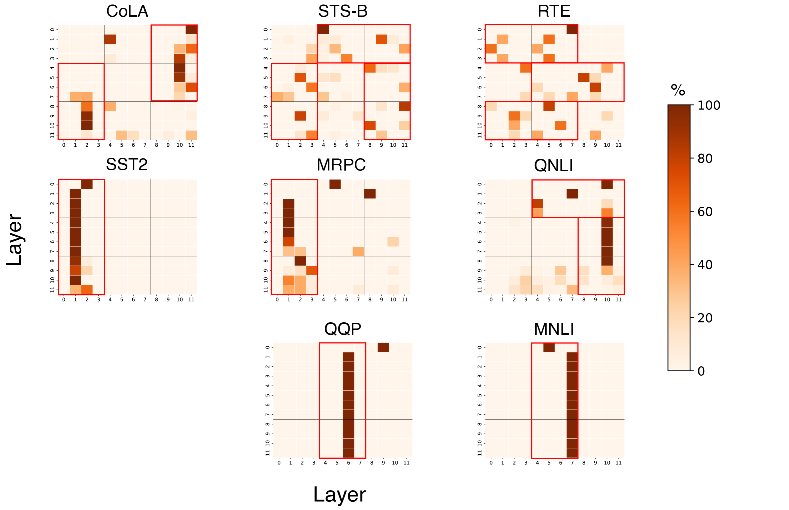
Figure 3: Plots of heat maps to visualize the percentage of time each layer expert is chosen at every layer of MoLEx when fine-tuning RoBERTa-base on all GLUE tasks. As one expert is fixed to be the original layer, the x-axis corresponds to the sequential layer while the y-axis corresponds to the layer experts. The darker a square is, the more often that layer is chosen by the gate during inference. For example, when fine-tuning on CoLA, layer 9 mixes with layer 2, 100% of the time. The grids are partitioned into thirds along the x-axis and y-axis for easy visualization of early, middle and later layers.

C.4 Linguistic Properties Captured by RoBERTa

In this section we will discuss the linguistic properties captured by RoBERTa as revealed through our probe analysis. We observe in Table 4 that across almost all probes, layer 11 does particularly well, suggesting that the last layer of the model encodes a considerable amount of general linguistic information. This is the main contrast to the probe analysis performed on BERT in (Jawahar et al., 2019) and could be an unintended consequence of the optimized training recipe in RoBERTa, highlighting how various training protocols can influence the learning outcomes of a model. It is also worth noting that all probes on RoBERTa, except for WC, performs roughly on the same scale as BERT while WC is much poorer in comparison, even with logistic regression. This could suggest that this surface level information is not relevant to the NLP in the model.

The remainder of the analysis corroborates with the probe analysis on BERT whereby the early layers contain superficial information, the middle layers, syntactic information and later layers, semantic. This further aligns with the intuition that more complex structures within the data are revealed deeper in the model as it undergoes more processing as discussed in Section 2.2.

Appendix D Ablation Study

Table 9 compares results on 3 GLUE tasks, CoLA, QQP, and SST-2 when using Top1 and Top2 routing. We observe that Top1 yields more improvement. Thus, we use a Top1 routing for our MoLEx models.

Table 9: Comparison of RoBERTa-base on GLUE tasks, CoLA, QQP and SST-2 when fine-tuned with MoLEx using Top-1 and Top-2 routing. We report accuracy for all tasks in the table below.

Method	CoLA	QQP	SST-2
MoLEx (Top1)	64.8 $\pm$.5	91.0 $\pm$.0	95.4 $\pm$.2
MoLEx (Top2)	63.7 $\pm$.4	90.7 $\pm$.0	95.0 $\pm$.3

Appendix E Additional Experimental Results and Efficency Analysis

E.1 Full parameter fine-tuning for RoBERTa

We conduct additional experiments for RoBERTa-base using full parameter fine-tuning on the GLUE benchmark. We present the results in Table 10 below. Our MoLEx model consistently outperforms the full parameter fine-tuning across all tasks. These findings further confirm MoLEx’s adaptability to different models and training methods.

Table 10: RoBERTa-base with full parameter fine-tuning and with MoLEx when fine-tuned on the GLUE benchmark. We report accuracy for all tasks except for, Pearson correlation for STS-B, Matthew’s correlation for CoLA and the overall (matched and mismatched) accuracy for MNLI. A higher value reflects a better performance of the model.

Method	RTE	MRPC	STS-B	CoLA	MNLI	QNLI	SST-2	QQP	Ave.
RoBERTa (full parameter)	80.1	88.7	90.9	62.6	87.7	92.9	95.0	91.8	86.2
RoBERTa (MoLEx)	80.9	89.5	91.1	63.3	87.8	93.1	95.1	91.8	86.6

E.2 Fine-tuning Llama-3.2-1B using LoRA

We conduct additional experiments to fine-tune Llama-3.2-1B on the Alpaca dataset using LoRA. We use the publicly available repository https://github.com/meta-llama/llama3 for our experiments and employ MoLEx to fine-tune the model in comparison with LoRA. As shown in Table 11, on this task with Llama-3.2-1B, MoLEx achieves better train and validation PPL than LoRA, demonstrating the effectiveness of MoLEx in large language models.

Further, we evaluate each model on the standard MMLU (Hendrycks et al., 2020), AGIEval English (Zhong et al., 2024), Hellaswag (Zellers et al., 2019), and ARC-Challenge dataset Clark et al. (2018) and report their results in Table 12. Consistent with our results on Alpaca, MoLEx improves over the naive LoRA model, confirming its advantage.

Table 11: Train and validation perplexity (PPL) when fine-tuning Llama-3.2-1B on Alpaca using LoRA and LoRA + MoLEx. Lower PPL is indicative of better performance.

Method	Train PPL ($\downarrow$)	Validation PPL ($\downarrow$)
LoRA	4.18	4.11
MoLEx	4.05	4.02

Table 12: Accuracy when evaluating Llama-3.2-1B on MMLU, AGIEval English, Hellaswag, and ARC-Challenge using LoRA and LoRA + MoLEx. A higher value is indicative of better performance.

Method	MMLU	AGIEval English	Hellaswag	ARC-Challenge
LoRA	30.42	19.16	47.14	36.69
MoLEx	31.51	19.81	48.23	37.80

E.3 Detailed Efficiency Analysis on Llama-3.2-1B

While more resources are required during inference in MoLEx as compared to the naive PEFT model, these can be accelerated during inference time through parallization. In this section, we include a more detailed efficiency analysis when implementing MoLEx in Llama-3.2-1B and using LoRA for fine-tuning on the Alpaca dataset.

As computational efficiency refers to the amount of time required for a given step in a calculation, we maintain that MoLEx is as efficient as the original method used without MoLEx. While MoLEx almost doubles the overall computational load (flops), there is only a minimal increase in inference time due to parallelization of the forward computations through two layers. We present our analysis in the Table 13 for a more detailed comparison with naive PEFT models.

Table 13: Efficiency analysis of Llama-3.2-1B fine-tuned using LoRA during inference on the Alpaca dataset with and without MoLEx implemented.

Method	Total	Trainable	Trainable	Memory	Flop/	Sec/	Flop/	Min/
	Parameters	Parameters	Parameters (%)	(MB)	Sample	Sample	Sec	Epoch
LoRA	1,236,666,368	851,968	0.0689	10,442	12.329 T	0.506	24.366 T	4:59
MoLEx	1,236,699,152	884,752	0.0715	10,442	22.511 T	0.557	40.415 T	6:00

References

- Adi et al. (2016) Yossi Adi, Einat Kermany, Yonatan Belinkov, Ofer Lavi, and Yoav Goldberg. Fine-grained analysis of sentence embeddings using auxiliary prediction tasks. arXiv preprint arXiv:1608.04207, 2016.
- Bar-Haim et al. (2006) Roy Bar-Haim, Ido Dagan, Bill Dolan, Lisa Ferro, and Danilo Giampiccolo. The second pascal recognising textual entailment challenge. Proceedings of the Second PASCAL Challenges Workshop on Recognising Textual Entailment, 01 2006.
- Belinkov & Glass (2019) Yonatan Belinkov and James Glass. Analysis methods in neural language processing: A survey. Transactions of the Association for Computational Linguistics, 7:49–72, 2019.
- Belinkov et al. (2017) Yonatan Belinkov, Nadir Durrani, Fahim Dalvi, Hassan Sajjad, and James Glass. What do neural machine translation models learn about morphology? In Regina Barzilay and Min-Yen Kan (eds.), Proceedings of the 55th Annual Meeting of the Association for Computational Linguistics (Volume 1: Long Papers), pp. 861–872, Vancouver, Canada, July 2017. Association for Computational Linguistics. doi: 10.18653/v1/P17-1080. URL https://aclanthology.org/P17-1080.
- Belinkov et al. (2018) Yonatan Belinkov, Lluís Màrquez, Hassan Sajjad, Nadir Durrani, Fahim Dalvi, and James Glass. Evaluating layers of representation in neural machine translation on part-of-speech and semantic tagging tasks. arXiv preprint arXiv:1801.07772, 2018.
- Bentivogli et al. (2009) Luisa Bentivogli, Bernardo Magnini, Ido Dagan, Hoa Trang Dang, and Danilo Giampiccolo. The fifth PASCAL recognizing textual entailment challenge. In Proceedings of the Second Text Analysis Conference, TAC 2009, Gaithersburg, Maryland, USA, November 16-17, 2009. NIST, 2009. URL https://tac.nist.gov/publications/2009/additional.papers/RTE5_overview.proceedings.pdf.
- Brown et al. (2020) Tom Brown, Benjamin Mann, Nick Ryder, Melanie Subbiah, Jared D Kaplan, Prafulla Dhariwal, Arvind Neelakantan, Pranav Shyam, Girish Sastry, Amanda Askell, et al. Language models are few-shot learners. Advances in neural information processing systems, 33:1877–1901, 2020.
- Cer et al. (2017) Daniel Cer, Mona Diab, Eneko Agirre, Iñigo Lopez-Gazpio, and Lucia Specia. SemEval-2017 task 1: Semantic textual similarity multilingual and crosslingual focused evaluation. In Steven Bethard, Marine Carpuat, Marianna Apidianaki, Saif M. Mohammad, Daniel Cer, and David Jurgens (eds.), Proceedings of the 11th International Workshop on Semantic Evaluation (SemEval-2017), pp. 1–14, Vancouver, Canada, August 2017. Association for Computational Linguistics. doi: 10.18653/v1/S17-2001. URL https://aclanthology.org/S17-2001.
- Chowdhery et al. (2023) Aakanksha Chowdhery, Sharan Narang, Jacob Devlin, Maarten Bosma, Gaurav Mishra, Adam Roberts, Paul Barham, Hyung Won Chung, Charles Sutton, Sebastian Gehrmann, et al. Palm: Scaling language modeling with pathways. Journal of Machine Learning Research, 24(240):1–113, 2023.
- Clark et al. (2018) Peter Clark, Isaac Cowhey, Oren Etzioni, Tushar Khot, Ashish Sabharwal, Carissa Schoenick, and Oyvind Tafjord. Think you have solved question answering? try arc, the ai2 reasoning challenge. ArXiv, abs/1803.05457, 2018. URL https://api.semanticscholar.org/CorpusID:3922816.
- Conneau & Kiela (2018) Alexis Conneau and Douwe Kiela. SentEval: An evaluation toolkit for universal sentence representations. In Nicoletta Calzolari, Khalid Choukri, Christopher Cieri, Thierry Declerck, Sara Goggi, Koiti Hasida, Hitoshi Isahara, Bente Maegaard, Joseph Mariani, Hélène Mazo, Asuncion Moreno, Jan Odijk, Stelios Piperidis, and Takenobu Tokunaga (eds.), Proceedings of the Eleventh International Conference on Language Resources and Evaluation (LREC 2018), Miyazaki, Japan, May 2018. European Language Resources Association (ELRA). URL https://aclanthology.org/L18-1269.
- Conneau et al. (2018) Alexis Conneau, German Kruszewski, Guillaume Lample, Loïc Barrault, and Marco Baroni. What you can cram into a single $&!#* vector: Probing sentence embeddings for linguistic properties. In Iryna Gurevych and Yusuke Miyao (eds.), Proceedings of the 56th Annual Meeting of the Association for Computational Linguistics (Volume 1: Long Papers), pp. 2126–2136, Melbourne, Australia, July 2018. Association for Computational Linguistics. doi: 10.18653/v1/P18-1198. URL https://aclanthology.org/P18-1198.
- Dagan et al. (2006) Ido Dagan, Oren Glickman, and Bernardo Magnini. The pascal recognising textual entailment challenge. In Joaquin Quiñonero-Candela, Ido Dagan, Bernardo Magnini, and Florence d’Alché Buc (eds.), Machine Learning Challenges. Evaluating Predictive Uncertainty, Visual Object Classification, and Recognising Tectual Entailment, pp. 177–190, Berlin, Heidelberg, 2006. Springer Berlin Heidelberg.
- Dalvi et al. (2017) Fahim Dalvi, Nadir Durrani, Hassan Sajjad, Yonatan Belinkov, and Stephan Vogel. Understanding and improving morphological learning in the neural machine translation decoder. In Greg Kondrak and Taro Watanabe (eds.), Proceedings of the Eighth International Joint Conference on Natural Language Processing (Volume 1: Long Papers), pp. 142–151, Taipei, Taiwan, November 2017. Asian Federation of Natural Language Processing. URL https://aclanthology.org/I17-1015.
- Devlin et al. (2018) Jacob Devlin, Ming-Wei Chang, Kenton Lee, and Kristina Toutanova. Bert: Pre-training of deep bidirectional transformers for language understanding. arXiv preprint arXiv:1810.04805, 2018.
- Doddington (2002) George Doddington. Automatic evaluation of machine translation quality using n-gram co-occurrence statistics. In Proceedings of the Second International Conference on Human Language Technology Research, HLT ’02, pp. 138–145, San Francisco, CA, USA, 2002. Morgan Kaufmann Publishers Inc.
- Dolan & Brockett (2005) William B. Dolan and Chris Brockett. Automatically constructing a corpus of sentential paraphrases. In Proceedings of the Third International Workshop on Paraphrasing (IWP2005), 2005. URL https://aclanthology.org/I05-5002.
- Du et al. (2022) Nan Du, Yanping Huang, Andrew M Dai, Simon Tong, Dmitry Lepikhin, Yuanzhong Xu, Maxim Krikun, Yanqi Zhou, Adams Wei Yu, Orhan Firat, Barret Zoph, Liam Fedus, Maarten P Bosma, Zongwei Zhou, Tao Wang, Emma Wang, Kellie Webster, Marie Pellat, Kevin Robinson, Kathleen Meier-Hellstern, Toju Duke, Lucas Dixon, Kun Zhang, Quoc Le, Yonghui Wu, Zhifeng Chen, and Claire Cui. GLaM: Efficient scaling of language models with mixture-of-experts. In Kamalika Chaudhuri, Stefanie Jegelka, Le Song, Csaba Szepesvari, Gang Niu, and Sivan Sabato (eds.), Proceedings of the 39th International Conference on Machine Learning, volume 162 of Proceedings of Machine Learning Research, pp. 5547–5569. PMLR, 17–23 Jul 2022. URL https://proceedings.mlr.press/v162/du22c.html.
- Fedus et al. (2022) William Fedus, Barret Zoph, and Noam Shazeer. Switch transformers: Scaling to trillion parameter models with simple and efficient sparsity. Journal of Machine Learning Research, 23(120):1–39, 2022.
- Ganaie et al. (2022) Mudasir A Ganaie, Minghui Hu, Ashwani Kumar Malik, Muhammad Tanveer, and Ponnuthurai N Suganthan. Ensemble deep learning: A review. Engineering Applications of Artificial Intelligence, 115:105151, 2022.
- Giampiccolo et al. (2007) Danilo Giampiccolo, Bernardo Magnini, Ido Dagan, and Bill Dolan. The third PASCAL recognizing textual entailment challenge. In Satoshi Sekine, Kentaro Inui, Ido Dagan, Bill Dolan, Danilo Giampiccolo, and Bernardo Magnini (eds.), Proceedings of the ACL-PASCAL Workshop on Textual Entailment and Paraphrasing, pp. 1–9, Prague, June 2007. Association for Computational Linguistics. URL https://aclanthology.org/W07-1401.
- Goldberg (2019) Yoav Goldberg. Assessing bert’s syntactic abilities. arXiv preprint arXiv:1901.05287, 2019.
- Gulordava (2018) K Gulordava. Colorless green recurrent networks dream hierarchically. arXiv preprint arXiv:1803.11138, 2018.
- Gupta et al. (2022) Neha Gupta, Jamie Smith, Ben Adlam, and Zelda Mariet. Ensembling over classifiers: a bias-variance perspective. arXiv preprint arXiv:2206.10566, 2022.
- Hambardzumyan et al. (2021) Karen Hambardzumyan, Hrant Khachatrian, and Jonathan May. WARP: Word-level Adversarial ReProgramming. In Chengqing Zong, Fei Xia, Wenjie Li, and Roberto Navigli (eds.), Proceedings of the 59th Annual Meeting of the Association for Computational Linguistics and the 11th International Joint Conference on Natural Language Processing (Volume 1: Long Papers), pp. 4921–4933, Online, August 2021. Association for Computational Linguistics. doi: 10.18653/v1/2021.acl-long.381. URL https://aclanthology.org/2021.acl-long.381.
- Hendrycks et al. (2020) Dan Hendrycks, Collin Burns, Steven Basart, Andy Zou, Mantas Mazeika, Dawn Xiaodong Song, and Jacob Steinhardt. Measuring massive multitask language understanding. ArXiv, abs/2009.03300, 2020. URL https://api.semanticscholar.org/CorpusID:221516475.
- Hewitt & Manning (2019) John Hewitt and Christopher D. Manning. A structural probe for finding syntax in word representations. In Jill Burstein, Christy Doran, and Thamar Solorio (eds.), Proceedings of the 2019 Conference of the North American Chapter of the Association for Computational Linguistics: Human Language Technologies, Volume 1 (Long and Short Papers), pp. 4129–4138, Minneapolis, Minnesota, June 2019. Association for Computational Linguistics. doi: 10.18653/v1/N19-1419. URL https://aclanthology.org/N19-1419.
- Houlsby et al. (2019) Neil Houlsby, Andrei Giurgiu, Stanislaw Jastrzebski, Bruna Morrone, Quentin De Laroussilhe, Andrea Gesmundo, Mona Attariyan, and Sylvain Gelly. Parameter-efficient transfer learning for nlp. In International conference on machine learning, pp. 2790–2799. PMLR, 2019.
- Hu et al. (2021) Edward J Hu, Yelong Shen, Phillip Wallis, Zeyuan Allen-Zhu, Yuanzhi Li, Shean Wang, Lu Wang, and Weizhu Chen. Lora: Low-rank adaptation of large language models. arXiv preprint arXiv:2106.09685, 2021.
- Hupkes et al. (2018) Dieuwke Hupkes, Sara Veldhoen, and Willem Zuidema. Visualisation and ‘diagnostic classifiers’ reveal how recurrent and recursive neural networks process hierarchical structure. J. Artif. Int. Res., 61(1):907–926, January 2018. ISSN 1076-9757.
- Jawahar et al. (2019) Ganesh Jawahar, Benoît Sagot, and Djamé Seddah. What does bert learn about the structure of language? In ACL 2019-57th Annual Meeting of the Association for Computational Linguistics, 2019.
- Kale & Rastogi (2020) Mihir Kale and Abhinav Rastogi. Text-to-text pre-training for data-to-text tasks. arXiv preprint arXiv:2005.10433, 2020.
- Komatsuzaki et al. (2022) Aran Komatsuzaki, Joan Puigcerver, James Lee-Thorp, Carlos Riquelme Ruiz, Basil Mustafa, Joshua Ainslie, Yi Tay, Mostafa Dehghani, and Neil Houlsby. Sparse upcycling: Training mixture-of-experts from dense checkpoints. arXiv preprint arXiv:2212.05055, 2022.
- Kumatani et al. (2021) Kenichi Kumatani, Robert Gmyr, Felipe Cruz Salinas, Linquan Liu, Wei Zuo, Devang Patel, Eric Sun, and Yu Shi. Building a great multi-lingual teacher with sparsely-gated mixture of experts for speech recognition. arXiv preprint arXiv:2112.05820, 2021.
- Lavie & Agarwal (2007) Alon Lavie and Abhaya Agarwal. METEOR: An automatic metric for MT evaluation with high levels of correlation with human judgments. In Chris Callison-Burch, Philipp Koehn, Cameron Shaw Fordyce, and Christof Monz (eds.), Proceedings of the Second Workshop on Statistical Machine Translation, pp. 228–231, Prague, Czech Republic, June 2007. Association for Computational Linguistics. URL https://aclanthology.org/W07-0734.
- Lawton et al. (2023) Neal Lawton, Anoop Kumar, Govind Thattai, Aram Galstyan, and Greg Ver Steeg. Neural architecture search for parameter-efficient fine-tuning of large pre-trained language models. arXiv preprint arXiv:2305.16597, 2023.
- Lepikhin et al. (2021) Dmitry Lepikhin, HyoukJoong Lee, Yuanzhong Xu, Dehao Chen, Orhan Firat, Yanping Huang, Maxim Krikun, Noam Shazeer, and Zhifeng Chen. {GS}hard: Scaling giant models with conditional computation and automatic sharding. In International Conference on Learning Representations, 2021. URL https://openreview.net/forum?id=qrwe7XHTmYb.
- Lester et al. (2021) Brian Lester, Rami Al-Rfou, and Noah Constant. The power of scale for parameter-efficient prompt tuning. arXiv preprint arXiv:2104.08691, 2021.
- Li & Liang (2021) Xiang Lisa Li and Percy Liang. Prefix-tuning: Optimizing continuous prompts for generation. In Chengqing Zong, Fei Xia, Wenjie Li, and Roberto Navigli (eds.), Proceedings of the 59th Annual Meeting of the Association for Computational Linguistics and the 11th International Joint Conference on Natural Language Processing (Volume 1: Long Papers), pp. 4582–4597, Online, August 2021. Association for Computational Linguistics. doi: 10.18653/v1/2021.acl-long.353. URL https://aclanthology.org/2021.acl-long.353.
- Lin (2004) Chin-Yew Lin. ROUGE: A package for automatic evaluation of summaries. In Text Summarization Branches Out, pp. 74–81, Barcelona, Spain, July 2004. Association for Computational Linguistics. URL https://aclanthology.org/W04-1013.
- Lin et al. (2020) Zhaojiang Lin, Andrea Madotto, and Pascale Fung. Exploring versatile generative language model via parameter-efficient transfer learning. In Trevor Cohn, Yulan He, and Yang Liu (eds.), Findings of the Association for Computational Linguistics: EMNLP 2020, pp. 441–459, Online, November 2020. Association for Computational Linguistics. doi: 10.18653/v1/2020.findings-emnlp.41. URL https://aclanthology.org/2020.findings-emnlp.41.
- Linzen et al. (2016) Tal Linzen, Emmanuel Dupoux, and Yoav Goldberg. Assessing the ability of lstms to learn syntax-sensitive dependencies. Transactions of the Association for Computational Linguistics, 4:521–535, 2016.
- Liu et al. (2019) Nelson F. Liu, Matt Gardner, Yonatan Belinkov, Matthew E. Peters, and Noah A. Smith. Linguistic knowledge and transferability of contextual representations. In Jill Burstein, Christy Doran, and Thamar Solorio (eds.), Proceedings of the 2019 Conference of the North American Chapter of the Association for Computational Linguistics: Human Language Technologies, Volume 1 (Long and Short Papers), pp. 1073–1094, Minneapolis, Minnesota, June 2019. Association for Computational Linguistics. doi: 10.18653/v1/N19-1112. URL https://aclanthology.org/N19-1112.
- Liu et al. (2023) Xiao Liu, Yanan Zheng, Zhengxiao Du, Ming Ding, Yujie Qian, Zhilin Yang, and Jie Tang. Gpt understands, too. AI Open, 2023.
- Liu (2020) Y Liu. Multilingual denoising pre-training for neural machine translation. arXiv preprint arXiv:2001.08210, 2020.
- Liu & Lapata (2019) Yang Liu and Mirella Lapata. Text summarization with pretrained encoders. In Kentaro Inui, Jing Jiang, Vincent Ng, and Xiaojun Wan (eds.), Proceedings of the 2019 Conference on Empirical Methods in Natural Language Processing and the 9th International Joint Conference on Natural Language Processing (EMNLP-IJCNLP), pp. 3730–3740, Hong Kong, China, November 2019. Association for Computational Linguistics. doi: 10.18653/v1/D19-1387. URL https://aclanthology.org/D19-1387.
- Liu (2019) Yinhan Liu. Roberta: A robustly optimized bert pretraining approach. arXiv preprint arXiv:1907.11692, 2019.
- Loshchilov (2017) I Loshchilov. Decoupled weight decay regularization. arXiv preprint arXiv:1711.05101, 2017.
- Marvin (2018) Rebecca Marvin. Targeted syntactic evaluation of language models. arXiv preprint arXiv:1808.09031, 2018.
- Matthews (1975) B.W. Matthews. Comparison of the predicted and observed secondary structure of t4 phage lysozyme. Biochimica et Biophysica Acta (BBA) - Protein Structure, 405(2):442–451, 1975. ISSN 0005-2795. doi: https://doi.org/10.1016/0005-2795(75)90109-9. URL https://www.sciencedirect.com/science/article/pii/0005279575901099.
- Mitchell et al. (2022) Eric Mitchell, Charles Lin, Antoine Bosselut, Chelsea Finn, and Christopher D Manning. Fast model editing at scale. In International Conference on Learning Representations, 2022. URL https://openreview.net/forum?id=0DcZxeWfOPt.
- Navon et al. (2023) Aviv Navon, Aviv Shamsian, Idan Achituve, Ethan Fetaya, Gal Chechik, and Haggai Maron. Equivariant architectures for learning in deep weight spaces. In International Conference on Machine Learning, pp. 25790–25816. PMLR, 2023.
- Nguyen et al. (2025) Viet Dung Nguyen, Minh Nguyen Hoang, Luc Nguyen, Rachel Teo, Tan Minh Nguyen, and Linh Duy Tran. CAMEx: Curvature-aware merging of experts. In The Thirteenth International Conference on Learning Representations, 2025. URL https://openreview.net/forum?id=nT2u0M0nf8.
- Nielsen et al. (2025) Stefan Nielsen, Rachel Teo, Laziz Abdullaev, and Tan Minh Nguyen. Tight clusters make specialized experts. In The Thirteenth International Conference on Learning Representations, 2025. URL https://openreview.net/forum?id=Pu3c0209cx.
- Novikova et al. (2017a) Jekaterina Novikova, Ondřej Dušek, and Verena Rieser. The E2E dataset: New challenges for end-to-end generation. In Kristiina Jokinen, Manfred Stede, David DeVault, and Annie Louis (eds.), Proceedings of the 18th Annual SIGdial Meeting on Discourse and Dialogue, pp. 201–206, Saarbrücken, Germany, August 2017a. Association for Computational Linguistics. doi: 10.18653/v1/W17-5525. URL https://aclanthology.org/W17-5525.
- Novikova et al. (2017b) Jekaterina Novikova, Ondřej Dušek, and Verena Rieser. The e2e dataset: New challenges for end-to-end generation. arXiv preprint arXiv:1706.09254, 2017b.
- Paperno et al. (2016) Denis Paperno, Germán Kruszewski, Angeliki Lazaridou, Quan Ngoc Pham, Raffaella Bernardi, Sandro Pezzelle, Marco Baroni, Gemma Boleda, and Raquel Fernández. The lambada dataset: Word prediction requiring a broad discourse context. arXiv preprint arXiv:1606.06031, 2016.
- Papineni et al. (2002) Kishore Papineni, Salim Roukos, Todd Ward, and Wei-Jing Zhu. Bleu: a method for automatic evaluation of machine translation. In Pierre Isabelle, Eugene Charniak, and Dekang Lin (eds.), Proceedings of the 40th Annual Meeting of the Association for Computational Linguistics, pp. 311–318, Philadelphia, Pennsylvania, USA, July 2002. Association for Computational Linguistics. doi: 10.3115/1073083.1073135. URL https://aclanthology.org/P02-1040.
- Peters et al. (2018) Matthew E. Peters, Mark Neumann, Luke Zettlemoyer, and Wen-tau Yih. Dissecting contextual word embeddings: Architecture and representation. In Ellen Riloff, David Chiang, Julia Hockenmaier, and Jun’ichi Tsujii (eds.), Proceedings of the 2018 Conference on Empirical Methods in Natural Language Processing, pp. 1499–1509, Brussels, Belgium, October-November 2018. Association for Computational Linguistics. doi: 10.18653/v1/D18-1179. URL https://aclanthology.org/D18-1179.
- Pfeiffer et al. (2021) Jonas Pfeiffer, Aishwarya Kamath, Andreas Rücklé, Kyunghyun Cho, and Iryna Gurevych. AdapterFusion: Non-destructive task composition for transfer learning. In Paola Merlo, Jorg Tiedemann, and Reut Tsarfaty (eds.), Proceedings of the 16th Conference of the European Chapter of the Association for Computational Linguistics: Main Volume, pp. 487–503, Online, April 2021. Association for Computational Linguistics. doi: 10.18653/v1/2021.eacl-main.39. URL https://aclanthology.org/2021.eacl-main.39.
- Qi et al. (2022) Wang Qi, Yu-Ping Ruan, Yuan Zuo, and Taihao Li. Parameter-efficient tuning on layer normalization for pre-trained language models. arXiv preprint arXiv:2211.08682, 2022.
- Radford et al. (2019) Alec Radford, Jeffrey Wu, Rewon Child, David Luan, Dario Amodei, Ilya Sutskever, et al. Language models are unsupervised multitask learners. OpenAI blog, 1(8):9, 2019.
- Raffel et al. (2020a) Colin Raffel, Noam Shazeer, Adam Roberts, Katherine Lee, Sharan Narang, Michael Matena, Yanqi Zhou, Wei Li, and Peter J. Liu. Exploring the limits of transfer learning with a unified text-to-text transformer. Journal of Machine Learning Research, 21(140):1–67, 2020a. URL http://jmlr.org/papers/v21/20-074.html.
- Raffel et al. (2020b) Colin Raffel, Noam Shazeer, Adam Roberts, Katherine Lee, Sharan Narang, Michael Matena, Yanqi Zhou, Wei Li, and Peter J Liu. Exploring the limits of transfer learning with a unified text-to-text transformer. Journal of machine learning research, 21(140):1–67, 2020b.
- Rajpurkar et al. (2018) Pranav Rajpurkar, Robin Jia, and Percy Liang. Know what you don’t know: Unanswerable questions for SQuAD. In Iryna Gurevych and Yusuke Miyao (eds.), Proceedings of the 56th Annual Meeting of the Association for Computational Linguistics (Volume 2: Short Papers), pp. 784–789, Melbourne, Australia, July 2018. Association for Computational Linguistics. doi: 10.18653/v1/P18-2124. URL https://aclanthology.org/P18-2124.
- Riquelme et al. (2021) Carlos Riquelme, Joan Puigcerver, Basil Mustafa, Maxim Neumann, Rodolphe Jenatton, André Susano Pinto, Daniel Keysers, and Neil Houlsby. Scaling vision with sparse mixture of experts. Advances in Neural Information Processing Systems, 34:8583–8595, 2021.
- Rücklé et al. (2021) Andreas Rücklé, Gregor Geigle, Max Glockner, Tilman Beck, Jonas Pfeiffer, Nils Reimers, and Iryna Gurevych. AdapterDrop: On the efficiency of adapters in transformers. In Marie-Francine Moens, Xuanjing Huang, Lucia Specia, and Scott Wen-tau Yih (eds.), Proceedings of the 2021 Conference on Empirical Methods in Natural Language Processing, pp. 7930–7946, Online and Punta Cana, Dominican Republic, November 2021. Association for Computational Linguistics. doi: 10.18653/v1/2021.emnlp-main.626. URL https://aclanthology.org/2021.emnlp-main.626.
- Sennrich (2017) Rico Sennrich. How grammatical is character-level neural machine translation? assessing MT quality with contrastive translation pairs. In Mirella Lapata, Phil Blunsom, and Alexander Koller (eds.), Proceedings of the 15th Conference of the European Chapter of the Association for Computational Linguistics: Volume 2, Short Papers, pp. 376–382, Valencia, Spain, April 2017. Association for Computational Linguistics. URL https://aclanthology.org/E17-2060.
- Shazeer et al. (2017) Noam Shazeer, *Azalia Mirhoseini, *Krzysztof Maziarz, Andy Davis, Quoc Le, Geoffrey Hinton, and Jeff Dean. Outrageously large neural networks: The sparsely-gated mixture-of-experts layer. In International Conference on Learning Representations, 2017. URL https://openreview.net/forum?id=B1ckMDqlg.
- Sinitsin et al. (2020) Anton Sinitsin, Vsevolod Plokhotnyuk, Dmitry Pyrkin, Sergei Popov, and Artem Babenko. Editable neural networks. In International Conference on Learning Representations, 2020. URL https://openreview.net/forum?id=HJedXaEtvS.
- Socher et al. (2013) Richard Socher, Alex Perelygin, Jean Wu, Jason Chuang, Christopher D. Manning, Andrew Ng, and Christopher Potts. Recursive deep models for semantic compositionality over a sentiment treebank. In David Yarowsky, Timothy Baldwin, Anna Korhonen, Karen Livescu, and Steven Bethard (eds.), Proceedings of the 2013 Conference on Empirical Methods in Natural Language Processing, pp. 1631–1642, Seattle, Washington, USA, October 2013. Association for Computational Linguistics. URL https://aclanthology.org/D13-1170.
- Stickland et al. (2020) Asa Cooper Stickland, Xian Li, and Marjan Ghazvininejad. Recipes for adapting pre-trained monolingual and multilingual models to machine translation. arXiv preprint arXiv:2004.14911, 2020.
- Tenney et al. (2019) Ian Tenney, Patrick Xia, Berlin Chen, Alex Wang, Adam Poliak, R Thomas McCoy, Najoung Kim, Benjamin Van Durme, Samuel R Bowman, Dipanjan Das, et al. What do you learn from context? probing for sentence structure in contextualized word representations. arXiv preprint arXiv:1905.06316, 2019.
- Teo & Nguyen (2024) Rachel Teo and Tan Minh Nguyen. MomentumSMoe: Integrating momentum into sparse mixture of experts. In The Thirty-eighth Annual Conference on Neural Information Processing Systems, 2024. URL https://openreview.net/forum?id=y929esCZNJ.
- Tran et al. (2025a) Hoang Tran, Thieu Vo, Tho Huu, Tan Nguyen, et al. Monomial matrix group equivariant neural functional networks. Advances in Neural Information Processing Systems, 37:48628–48665, 2025a.
- Tran et al. (2025b) Hoang V. Tran, Thieu Vo, An Nguyen The, Tho Tran Huu, Minh-Khoi Nguyen-Nhat, Thanh Tran, Duy-Tung Pham, and Tan Minh Nguyen. Equivariant neural functional networks for transformers. In The Thirteenth International Conference on Learning Representations, 2025b. URL https://openreview.net/forum?id=uBai0ukstY.
- Vedantam et al. (2015) Ramakrishna Vedantam, C. Lawrence Zitnick, and Devi Parikh. Cider: Consensus-based image description evaluation. In 2015 IEEE Conference on Computer Vision and Pattern Recognition (CVPR), pp. 4566–4575, 2015. doi: 10.1109/CVPR.2015.7299087.
- Vo et al. (2024) Thieu N Vo, Viet-Hoang Tran, Tho Tran Huu, An Nguyen The, Thanh Tran, Minh-Khoi Nguyen-Nhat, Duy-Tung Pham, and Tan Minh Nguyen. Equivariant polynomial functional networks. arXiv preprint arXiv:2410.04213, 2024.
- Wang et al. (2018) Alex Wang, Amanpreet Singh, Julian Michael, Felix Hill, Omer Levy, and Samuel Bowman. GLUE: A multi-task benchmark and analysis platform for natural language understanding. In Tal Linzen, Grzegorz Chrupała, and Afra Alishahi (eds.), Proceedings of the 2018 EMNLP Workshop BlackboxNLP: Analyzing and Interpreting Neural Networks for NLP, pp. 353–355, Brussels, Belgium, November 2018. Association for Computational Linguistics. doi: 10.18653/v1/W18-5446. URL https://aclanthology.org/W18-5446.
- Warstadt et al. (2019) Alex Warstadt, Amanpreet Singh, and Samuel R. Bowman. Neural network acceptability judgments. Transactions of the Association for Computational Linguistics, 7:625–641, 2019. doi: 10.1162/tacl˙a˙00290. URL https://aclanthology.org/Q19-1040.
- Williams et al. (2018) Adina Williams, Nikita Nangia, and Samuel Bowman. A broad-coverage challenge corpus for sentence understanding through inference. In Marilyn Walker, Heng Ji, and Amanda Stent (eds.), Proceedings of the 2018 Conference of the North American Chapter of the Association for Computational Linguistics: Human Language Technologies, Volume 1 (Long Papers), pp. 1112–1122, New Orleans, Louisiana, June 2018. Association for Computational Linguistics. doi: 10.18653/v1/N18-1101. URL https://aclanthology.org/N18-1101.
- Wolf et al. (2020) Thomas Wolf, Lysandre Debut, Victor Sanh, Julien Chaumond, Clement Delangue, Anthony Moi, Pierric Cistac, Tim Rault, Remi Louf, Morgan Funtowicz, Joe Davison, Sam Shleifer, Patrick von Platen, Clara Ma, Yacine Jernite, Julien Plu, Canwen Xu, Teven Le Scao, Sylvain Gugger, Mariama Drame, Quentin Lhoest, and Alexander Rush. Transformers: State-of-the-art natural language processing. In Qun Liu and David Schlangen (eds.), Proceedings of the 2020 Conference on Empirical Methods in Natural Language Processing: System Demonstrations, pp. 38–45, Online, October 2020. Association for Computational Linguistics. doi: 10.18653/v1/2020.emnlp-demos.6. URL https://aclanthology.org/2020.emnlp-demos.6.
- Xu et al. (2023) Lingling Xu, Haoran Xie, Si-Zhao Joe Qin, Xiaohui Tao, and Fu Lee Wang. Parameter-efficient fine-tuning methods for pretrained language models: A critical review and assessment. arXiv preprint arXiv:2312.12148, 2023.
- Zaken et al. (2021) Elad Ben Zaken, Shauli Ravfogel, and Yoav Goldberg. Bitfit: Simple parameter-efficient fine-tuning for transformer-based masked language-models. arXiv preprint arXiv:2106.10199, 2021.
- Zellers et al. (2019) Rowan Zellers, Ari Holtzman, Yonatan Bisk, Ali Farhadi, and Yejin Choi. Hellaswag: Can a machine really finish your sentence? In Annual Meeting of the Association for Computational Linguistics, 2019. URL https://api.semanticscholar.org/CorpusID:159041722.
- Zhang et al. (2020) Yizhe Zhang, Siqi Sun, Michel Galley, Yen-Chun Chen, Chris Brockett, Xiang Gao, Jianfeng Gao, Jingjing Liu, and Bill Dolan. DIALOGPT : Large-scale generative pre-training for conversational response generation. In Asli Celikyilmaz and Tsung-Hsien Wen (eds.), Proceedings of the 58th Annual Meeting of the Association for Computational Linguistics: System Demonstrations, pp. 270–278, Online, July 2020. Association for Computational Linguistics. doi: 10.18653/v1/2020.acl-demos.30. URL https://aclanthology.org/2020.acl-demos.30.
- Zhang et al. (2023) Zhen-Ru Zhang, Chuanqi Tan, Haiyang Xu, Chengyu Wang, Jun Huang, and Songfang Huang. Towards adaptive prefix tuning for parameter-efficient language model fine-tuning. arXiv preprint arXiv:2305.15212, 2023.
- Zhong et al. (2020) Ming Zhong, Pengfei Liu, Yiran Chen, Danqing Wang, Xipeng Qiu, and Xuanjing Huang. Extractive summarization as text matching. In Dan Jurafsky, Joyce Chai, Natalie Schluter, and Joel Tetreault (eds.), Proceedings of the 58th Annual Meeting of the Association for Computational Linguistics, pp. 6197–6208, Online, July 2020. Association for Computational Linguistics. doi: 10.18653/v1/2020.acl-main.552. URL https://aclanthology.org/2020.acl-main.552.
- Zhong et al. (2024) Wanjun Zhong, Ruixiang Cui, Yiduo Guo, Yaobo Liang, Shuai Lu, Yanlin Wang, Amin Saied, Weizhu Chen, and Nan Duan. AGIEval: A human-centric benchmark for evaluating foundation models. In Kevin Duh, Helena Gomez, and Steven Bethard (eds.), Findings of the Association for Computational Linguistics: NAACL 2024, pp. 2299–2314, Mexico City, Mexico, June 2024. Association for Computational Linguistics. doi: 10.18653/v1/2024.findings-naacl.149. URL https://aclanthology.org/2024.findings-naacl.149.
- Zhou et al. (2023a) Allan Zhou, Kaien Yang, Kaylee Burns, Adriano Cardace, Yiding Jiang, Samuel Sokota, J Zico Kolter, and Chelsea Finn. Permutation equivariant neural functionals. Advances in neural information processing systems, 36:24966–24992, 2023a.
- Zhou et al. (2023b) Allan Zhou, Kaien Yang, Yiding Jiang, Kaylee Burns, Winnie Xu, Samuel Sokota, J Zico Kolter, and Chelsea Finn. Neural functional transformers. Advances in neural information processing systems, 36:77485–77502, 2023b.
- Zhou et al. (2023c) Yanqi Zhou, Nan Du, Yanping Huang, Daiyi Peng, Chang Lan, Da Huang, Siamak Shakeri, David So, Andrew M. Dai, Yifeng Lu, Zhifeng Chen, Quoc V Le, Claire Cui, James Laudon, and Jeff Dean. Brainformers: Trading simplicity for efficiency. In Andreas Krause, Emma Brunskill, Kyunghyun Cho, Barbara Engelhardt, Sivan Sabato, and Jonathan Scarlett (eds.), Proceedings of the 40th International Conference on Machine Learning, volume 202 of Proceedings of Machine Learning Research, pp. 42531–42542. PMLR, 23–29 Jul 2023c. URL https://proceedings.mlr.press/v202/zhou23c.html.
- Zhu et al. (2020) Jinhua Zhu, Yingce Xia, Lijun Wu, Di He, Tao Qin, Wengang Zhou, Houqiang Li, and Tie-Yan Liu. Incorporating bert into neural machine translation. arXiv preprint arXiv:2002.06823, 2020.
- Zhu (2015) Yukun Zhu. Aligning books and movies: Towards story-like visual explanations by watching movies and reading books. arXiv preprint arXiv:1506.06724, 2015.