Magnon thermal conductivity in multiferroics with spin cycloids
Abstract
Multiferroic materials, characterized by the occurrence of two or more ferroic properties, hold potential in future technological applications and also exhibit intriguing phenomena caused by the interplay of multiple orders. One such example is the formation of spin cycloid structures within multiferroic materials, which we investigate in this work by focusing on their magnon excitations and transport based on a general multiferroic Hamiltonian with an antiferromagnetic order. More specifically, we identify the ground state and explore the dynamics of magnon modes, revealing distinct in-plane and out-of-plane modes with anisotropic dispersion relations. The magnon modes include a massless excitation, known as the Goldstone boson, originating from the spontaneous breaking of the translational symmetry by the formation of the cycloid structures. By employing the Boltzmann transport formalism, the magnonic thermal conductivity with spin cycloids and low-temperature anisotropic behaviors is discussed. This work provides pathways to envision the spin-textured multiferroics, which may serve as a fertile ground to look for novel thermal and spin transport with the rich interplay of quasiparticles such as magnons and phonons.
I Introduction
Multiferroics refer to substances that exhibit more than one order parameter, the study of which has formed a rapidly advancing field within materials science and spintronics [1, 2]. The combination of multiple order parameters confers novel functionalities upon these materials, fostering potential applications in diverse fields, such as memory devices and sensors [3, 4, 5]. Currently, extensive research efforts are underway to explore multiferroics across various substances, prominently the bismuth ferrite BiFeO3 (BFO) that harbors ferroelectricity and antiferromagnetism simultaneously at room temperature [6, 7, 8, 9, 10, 11]. One reason why multiferroics are attracting significant attention is that they enable the control of magnetism through an electric field [12, 13, 14, 15, 16]. In the case of typical antiferromagnets, the magnetic moments of the sublattices cancel each other out, making it challenging to manipulate and detect the magnetic order parameters for device applications. However, in multiferroics, the antiferromagnetic order that can be modulated and probed by electrical means through magnetoelectric coupling associated with the two coexisting order parameters [17, 18, 19, 20].
In contrast to conventional ferromagnetic or ferroelectric materials where ground states are often uniform, multiferroic materials tend to exhibit a distinct ground state [21]. Among the intriguing phenomena observed within various multiferroics, including BFO, is the manifestation of spin cycloid structures, characterized by the helical modulation of magnetic orders caused by the inversion-symmetry breaking associated with the electric polarization [22, 10, 11, 23]. Understanding such spin cycloidal structures and their effects on other physical properties such as heat and spin transport is crucial to elucidate the mechanisms underlying various phenomena occurring in multiferroic materials and also to their practical use [18, 24, 19, 25].
In this work, we provide a theoretical framework of the magnon transport in magnetoelectric multiferroics. Based on a general Landau-Ginzburg formalism for multiferroics with antiferromagnetic orders, we obtain the ground states and determine the associated magnon band structure in the presence of an external magnetic field. The magnon band structure manifests the anisotropy in the spin cycloid structure. Along the direction of the order parameter winding, the spin cycloid defines a spatial period that imprints on the magnon bands, which results in a gap opening at the magnetic Brillouin zone boundary. The thermal transport conducted by magnons also shows an anisotropy, offering a transport probe of the microscopic spin cycloid texture. In addition, the dependence of the magnonic thermal conductivity on the magnetic field reveals the field-induced change of the underlying spin-cycloid structure, providing a way to probe the elusive background spin texture.
The remaining sections of the paper are organized as follows. In Sec. II, the model to calculate the thermal conductivity in multiferroics is described. In Sec. III, we discussed the results of the ground state of the systems, and use these results to calculate the excitations and anisotropic thermal conductivity followed by the conclusion Sec. IV.
II Model
In this section, we elucidate the model construction of multiferroic materials, utilizing the Landau-Ginzberg free-energy density, represented as [26, 27, 11, 28]
| (1) |
where is the antiferromagnetic vector, which has unit length and is magnetization vector. Additionally, the free energy is associated with the ferroelectric polarization . The first term accounts for the exchange interaction, while the second term represents the suppression of the magnetization associated with antiferromagnetism. The third and fourth terms embody the Lifshitz invariant and Dzyaloshinskii–Moriya interaction, respectively. The origin of the third term is the interaction between the electric polarization associated with the underlying ferroelectric order and the electric polarization induced by the magnetic texture [29, 30]. The fourth term arises when inversion symmetry is broken in the crystal structure. Note that, in the case of BFO, oxygen octahedral tilts involve symmetry breakings that yield the occurrence of Dzyaloshinskii-Moriya interactions (DMI) [31, 32, 33, 11]. Nevertheless, since these octahedral tilts are known to be strongly coupled to the polarization [34], it is usually sufficient to include in a basic model. Finally, the fifth and last term introduce single-ion easy-axis anisotropy and Zeeman coupling to an external magnetic field , respectively. The inspiration behind the formulation of the aforementioned free energy (II) stems from the Hamiltonian of multiferroic materials, such as BFO [31, 11]. In our work, it is assumed that is aligned along the z-direction and has a fixed magnitude and that the Dzyaloshinskii–Moriya vector is in the -direction [11].
By employing the aforementioned free energy (II), we derive the Lagrangian density for the system:
| (2) |
In this expression, the first term represents the kinetic term of the magnetic system [35, 36], while the subsequent terms denote the potential terms. Since the electric polarization and other structural distortions are assumed to be fixed, the dynamical term of is neglected. By employing the Euler-Lagrange equations and information regarding the ground state, we derive the dynamics of magnons from the Lagrangian (II).
III Result
In this section, we present the findings of our investigation into the multiferroic model that we constructed. We begin by determining its ground state of given free energy, followed by an exploration of excitations within the system and an analysis of its thermal conductivity.
III.1 Ground state
To determine the ground state, we minimize the Landau-Ginzburg free energy under constraints and . The original constraint is , but under the assumption that the magnetization is very small, it simplifies to . For convenience, let us parameterize and as and , where and . In the models we are letting and . Then, the free-energy density in terms of the four dynamic variables is given by
| (3) |
Solving the Euler-Lagrange equation for given free energy (III.1) about and yields the following solutions:
| (4) | |||
| (5) | |||
| (6) | |||
| (7) |
This solution creates a spin cycloid structure on the plane which is spanned by the z-axis and one specific direction in the -plane. Here, we can see that the term can be interpreted as the effective anisotropy of the system, leading us to define it as . The spin cycloid structure can be analytically obtained using Jacobi elliptic functions :
| (8) | ||||
| (9) |
for the case, and
| (10) | ||||
| (11) |
for the case where C is the integration constant determined by minimizing the total free energy of the system. This is one of our main results: the analytical solution for spin cycloids of multiferroic materials [Eq. (II)] in the presence of an external magnetic field . We note here that our solution generalizes the known results in the absence of a magnetic field which can be found in Refs. [11, 28, 23].
Note that the DMI and the magnetic field enter as a quadratic order term in Eq. (7) with a negative sign and counteract the easy-axis anisotropy and therefore can be interpreted as an effective easy-plane anisotropy. In particular, one special case occurs when the effective anisotropy vanishes, , which yields:
| (12) |
This defines a critical magetic field , where the anharmonic effects vanish and therefore becomes linearly dependent on (see Eq. (7)).
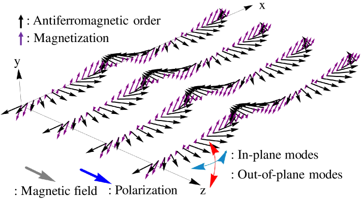
Without loss of generality, let us assume , implying that the spin cycloid structure lies along the -direction. Then, can be simply replaced by and consequently, the antiferromagnetic vector of the spin cycloid structure rotates within the -plane. Moreover, if there is no external magnetic field the magnetization vector aligns along the -direction, exhibiting the identical periodicity as the spin cycloid structure. The magnitude of is fully determined by the cycloid structure. In this case, it is evident that the and vectors exhibit no dependence on the -direction. The ground state of the system within the -plane is illustrated in Fig. 1. Upon inserting the values from Table. 1 for verification, it is observed that the value of is approximately 20 times smaller than . Hence, it can be inferred that there is a consistency with the assumed constraint, which establishes the antiferromagnetic nature of the material.
III.2 Magnon excitation
Form the Eq. (II) and Eq. (III.1), the Euler-Lagrange equation for can be derived as
| (13) | ||||
| (14) | ||||
| (15) | ||||
| (16) |
in spherical coordinates. To obtain the spin-wave solution for small deviations from the ground state, we set
where the subscript refers to the configuration of the ground state, while , and indicate the small deviations of the corresponding quantities from the ground state.
Next, we expand the above Eqs. (13-16) up to linear order in , , , and . To find the spin wave dynamics, we use the separation of variables method. As described above, we set the ground state of the system to have the -directional spin cycloid structure. Thus, we take . Rotating about the z-axis by radians allows us to represent the remaining cases () as well. Applying the ansatz , the equations are simplified. In the case of uniform distribution along y-axis, such as in a thin film in the xz-palne, setting , we obtain the following expression :
| (17) | ||||
| (18) | ||||
| (19) | ||||
| (20) |
where . Then, Eq. (17) and Eq. (18) allow us to recognize two different modes of excitations. Equation (17) describes the in-plane oscillation of the vector within the cycloid plane, referred to as the in-plane mode. Equation (18) depicts the out-of-plane oscillation of the vector perpendicular to the cycloid plane, referred to as the out-of-plane mode. A schematic picture of both modes can be found in Fig. 1. Additionally, knowing the in-plane and out-of-plane modes provides complete information about the dynamics of the magnetization vector, as described by Eq. (19) and Eq. (20).
Dispersion relation of in-plane mode can be obtained analytically by solving the Lamé equation (21) for , , , and :
| (21) |
The analytic solution of the excitation mode of Eq. (17) is given by :
| (22) |
where , , and are Jacobi’s eta, theta and zeta functions [37, 38, 39]. In Eq. (22), with the choice where dn is delta amplitude. Since the potential is a periodic function, the solution must also be a periodic function by the Bloch theorem. In this case, the period of the potential is half that of the spin cycloid. Therefore, is pure imaginary and the value for the function can be determinded.
To obtain the dispersion relation of out-of-plane mode, we need to solve eigenvalue problem Eq. (18). In this case, utilizing the periodicity of the spin structure, it is possible to determine the excitation, referred to as the central equation [40, 41].
| (23) |
where , , and , are respectively the periodic function, wavelength of the given periodic function and eigenvalue. Here, the wavelength of the periodic function is half the wavelength of the spin cycloid. Using the Fourier transformation,
| (24) | ||||
| (25) | ||||
| (26) |
where . We obtained the following equation.
| (27) |
Each Fourier component must have the same value on both sides, thus the central equation becomes
| (28) |
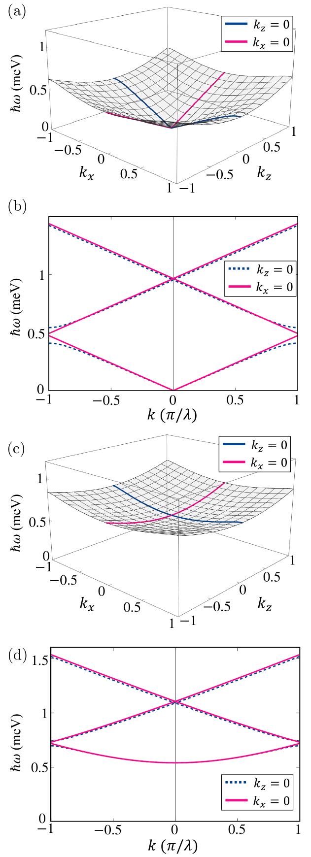
Solving Eq. (17) using the central equation method or solving the Lamé equation analytically, both yield the same dispersion relation. However, we were unable to to find the closed-form solution of Eq. (18), so we obtain its dispersion relation numerically by solving the central equation. The values used in the numerical calculations are those for BFO [11] given in Table. 1. Using the parameters in Table. 1 in numerical computations, we generate Fig. 2. The wavelength and are determined during the process of minimizing the average free energy density.
| Parameter | Value |
|---|---|
| erg cm-3 | |
| erg cm-2 | |
| erg cm-3 | |
| A | erg cm-1 |
| erg-1 cm3 | |
| erg s cm-3 |
In Fig. 2, we observe the anisotropy of the bands. The magnon band in the -direction (with ) exhibits a gap at the Brillouin-zone boundary which arises due to the periodcity of the spin cycloid, while the magnon band in the -direction (with ) does not have a gap. Note that the gap exists only between the lowest band and the second lowest band in the -direction band (with ) for both modes, i.e. at higher bands, no gaps are observed at the boundary or center of the Brillouin zone in the -direction. The magnon band in the -direction in-plane mode follows a normal antiferromagnetic dispersion relation.
Another noteworthy point is that the in-plane mode represents a massless excitation (Fig. 2(b)). The gapless at the zone center is the Goldstone mode associated with the spontaneous symmetry breaking. In the ground state depicted in Fig. 1, translational symmetry in the -direction is broken by the magnetic ground state, while it remains preserved in the Hamiltonian state. Hence, in this model, spontaneous symmetry breaking occurs, and the in-plane mode of magnons corresponds to the Goldstone boson.
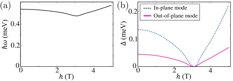
Figure 3 illustrates how the band gap changes with the magnetic field. At the center of the Brillouin zone, the in-plane mode always has zero energy, while the out-of-plane mode reaches its minimum value at the critical field, determined by , which is about for BFO, and increases on either side of this field as shown in Fig. 3(a). At the critical field, the gap at the Brillouin-zone center has the value , which is about 0.5 for BFO. Figure 3(b) shows the gap between the lowest and the second lowest band at the boundary of the Brillouin zone along x, where the gap closes at the critical field but opens and increases as one moves away from the critical field. This implies that the anisotropy inherent in the material can be controlled via the magnetic field. The field dependence of the gap as a function of a magnetic field is one of our key findings of this work.
III.3 Magnon thermal conductivity
We utilize the Boltzmann transport equation within the relaxation time approximation to investigate thermal conductivity of thermal magnon. The equation takes the form
| (29) |
Here, denotes the relaxation time, and and represent the magnon distribution functions of the non-equilibrium and equilibrium states, respectively, where . Focusing on the stationary , i.e., . The Boltzmann equation is simplified to
| (30) |
Assuming that the thermal gradient of the given sample is sufficiently small, the non-equilibrium distribution function can be understood as a small variation from the equilibrium distribution function and can be expressed as
| (31) |
Then, after combining it with Boltzmann transport equation, we can obtain
| (32) |
Under the assumption that the thermal gradient of the given sample is sufficiently small, can be ignored to compare , leading to the following result.
| (33) |
The heat flux flowing in the direction is
| (34) |
And we know that , where
| (35) |
In numerical calculations, the magnon velocity is defined as and the relaxation time is assumed to be constant at .
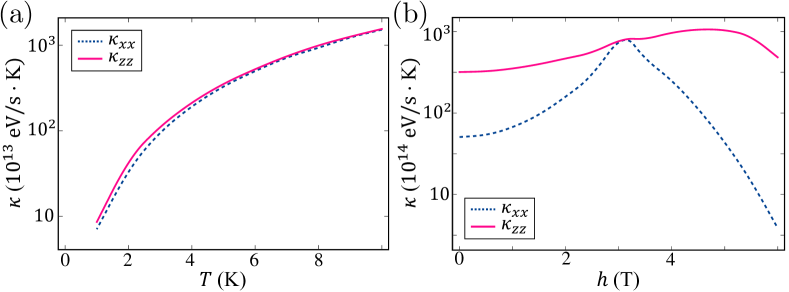
In Fig. 4(a), the numerical result demonstrates anisotropy of thermal conductivity between the - and -directions. The anisotropy of thermal conductivity is most noticeable at low temperatures because anisotropy of band is most pronounced in the lowest band, becoming less prominent in higher bands as the band gap and anisotropy become negligible relative to the temperature scale. In other words, as we move towards higher temperatures, the contribution of bands with reduced anisotropy to thermal conductivity increases, leading to diminished anisotropy of thermal conductivity. In Fig. 4(b), we can see that the thermal conductivity changes as a function of the magnetic field. This shows that the anisotropy, governed by the magnetic field, also affects transport properties. In particular, shows the peak around the critical field , which stems from the field dependence of the magnon bands shown in Fig. 3(b) and therefore can be used to infer the underlying spin-cycloid structures.
IV Conclusion
We have investigated the spin-cycloid ground states and the spin-wave excitations of multiferroic antiferromagnets, taking BFO as a paradigmatic example of an antiferromagnetic material in which an inversion-symmetry-breaking distortion can induce a spin cycloid. Our analysis has revealed the two distinct modes of excitations within the band structure, including one massless excitation, attributed to the Goldstone boson resulting from spontaneous translational symmetry breaking of the ground-state spin cycloid that exhibits gap opening at the magnetic Brillouin zone boundary. We have found that the effect of the DMI and the magnetic field (aligned with the polarization vector) on the dynamics of magnons can be interpreted as the effect of the effective easy-plane anisotropy. To study the transport properties, the Boltzmann transport equation under the relaxation time approximation is used to investigate thermal conductivity. Our numerical results have shown the anisotropy in thermal conductivity, particularly at low temperatures, which is attributed to the pronounced anisotropy in the band structure. However, at higher temperatures, the contribution of bands with reduced anisotropy becomes more significant, resulting in diminished overall anisotropy in thermal conductivity. These findings highlight the temperature-dependent anisotropic behavior of thermal conductivity. We have also investigated the magnetic field dependence of the magnon bands and the thermal conductivity. These findings contribute to the understanding of multiferroic materials, shedding light on the dynamics and behaviors of magnons within these complex systems.
Acknowledgements.
H.W.P. and S.K.K. were supported by Brain Pool Plus Program through the National Research Foundation of Korea funded by the Ministry of Science and ICT (NRF-2020H1D3A2A03099291), by the National Research Foundation of Korea (NRF) grant funded by the Korea government (MSIT) (NRF-2021R1C1C1006273), and by the National Research Foundation of Korea funded by the Korea Government via the SRC Center for Quantum Coherence in Condensed Matter (NRF-RS-2023-00207732). S. Z. is supported by the Leibniz Association through the Leibniz Competition Project No. J200/2024. S.H. and R.R. acknowledge funding from the U.S. Department of Energy, Office of Basic Energy Sciences, Materials Sciences and Engineering Division under Contract No. DE-AC02-05-CH11231 (Codesign of Ultra-Low-Voltage Beyond CMOS Microelectronics) for the development of materials for low-power microelectronics. M.R. S.H., and R.R. acknowledge Air Force Office of Scientific Research 2D Materials and Devices Research program through Clarkson Aerospace Corp under Grant No. FA9550-21-1-0460. S.H. and R.R. also acknowledge the ARO-CHARM program as well as the NSF-FUSE program. We also acknowledge the Army Research Laboratory and was accomplished under Cooperative Agreement Number W911NF-24-2-0100. The views and conclusions contained in this document are those of the authors and should not be interpreted as representing the official policies, either expressed or implied, of the Army Research Laboratory or the U.S. Government. The U.S. Government is authorized to reproduce and distribute reprints for Government purposes notwithstanding any copyright notation herein. J.Í.-G. acknowledges the financial support from the Luxembourg National Research Fund through grant C21/MS/15799044/FERRODYNAMICS.References
- Smolenski and Chupis [1982] G. A. Smolenski and I. E. Chupis, Ferroelectromagnets, Sov. Phys. Usp. 25, 475 (1982).
- Eerenstein et al. [2006] W. Eerenstein, N. D. Mathur, and J. F. Scott, Multiferroic and magnetoelectric materials, Nature 442, 759 (2006).
- Bibes and Barthélémy [2008] M. Bibes and A. Barthélémy, Towards a magnetoelectric memory, Nat. Mater. 7, 425 (2008).
- Heron et al. [2014] J. T. Heron, J. L. Bosse, Q. He, Y. Gai, M. Trassin, L. Ye, J. D. Clarkson, C. Wang, J. Liu, S. Salahuddin, D. C. Ralph, D. G. Schlom, J. Íñiguez, B. D. Huey, and R. Ramesh, Deterministic switching of ferromagnetism at room temperature using an electric field, Nature 516, 370 (2014).
- Spaldin and Ramesh [2019] N. A. Spaldin and R. Ramesh, Advances in magnetoelectric multiferroics, Nat. Mater. 18, 203 (2019).
- Wang et al. [2012] D. Wang, J. Weerasinghe, and L. Bellaiche, Atomistic molecular dynamic simulations of multiferroics, Phys. Rev. Lett. 109, 067203 (2012).
- Moreau et al. [1971] J. M. Moreau, C. Michel, R. Gerson, and W. J. James, Ferroelectric x-ray and neutron diffraction study, J. Phys. Chem. Solids 32, 1315 (1971).
- Haumont et al. [2006] R. Haumont, J. Kreisel, P. Bouvier, and F. Hippert, Phonon anomalies and the ferroelectric phase transition in multiferroic , Phys. Rev. B 73, 132101 (2006).
- Wang et al. [2003] J. Wang, J. B. Neaton, H. Zheng, V. Nagarajan, S. B. Ogale, B. Liu, D. Viehland, V. Vaithyanathan, D. G. Schlom, U. V. Waghmare, N. A. Spaldin, K. M. Rabe, M. Wuttig, and R. Ramesh, Epitaxial multiferroic thin film heterostructures, Science 299, 1719 (2003).
- Kadomtseva et al. [2006] A. M. Kadomtseva, Y. F. Popov, A. P. Pyatakov, G. P. Vorobev, A. K. Zvezdin, and D. Viehland, Phase transitions in multiferroic BiFeO3 crystals, thin-layers, and ceramics: enduring potential for a single phase, room-temperature magnetoelectric ”holy grail”, Phase Transitions 79, 1019 (2006).
- Park et al. [2014] J. G. Park, M. D. Le, J. Jeong, and S. Lee, Structure and spin dynamics of multiferroic BiFeO3, J. Phys.: Condens. Matter 26, 433202 (2014).
- Lebeugle et al. [2008] D. Lebeugle, D. Colson, A. Forget, M. Viret, A. M. Bataille, and A. Gukasov, Electric-field-induced spin flop in single crystals at room temperature, Phys. Rev. Lett. 100, 227602 (2008).
- Gross et al. [2017] I. Gross, W. Akhtar, V. Garcia, L. J. Martínez, S. Chouaieb, K. Garcia, C. Carrétéro, A. Barthélémy, P. Appel, P. Maletinsky, J. V. Kim, J. Y. Chauleau, N. Jaouen, M. Viret, M. Bibes, S. Fusil, and V. Jacques, Real-space imaging of non-collinear antiferromagnetic order with a single-spin magnetometer, Nature 549, 252–256 (2017).
- Zhao et al. [2006] T. Zhao, A. Scholl, F. Zavaliche, K. Lee, M. Barry, A. Doran, M. P. Cruz, Y. H. Chu, C. Ederer, N. A. Spaldin, R. R. Das, D. M. Kim, S. H. Baek, C. B. Eom, and R. Ramesh, Electrical control of antiferromagnetic domains in multiferroic BiFeO3 films at room temperature, Nat. Mater. 5, 823–829 (2006).
- Haykal et al. [2020] A. Haykal, J. Fischer, W. Akhtar, J. Y. Chauleau, D. Sando, A. Finco, F. Godel, Y. A. Birkhölzer, C. Carrétéro, N. Jaouen, M. Bibes, M. Viret, S. Fusil, V. Jacques, and V. Garcia, Antiferromagnetic textures in BiFeO3 controlled by strain and electric field, Nat. Commun. 11, 1704 (2020).
- Meisenheimer et al. [2024] P. Meisenheimer, G. Moore, S. Zhou, H. Zhang, X. Huang, S. Husain, X. Chen, L. W. Martin, K. A. Persson, S. Griffin, L. Caretta, P. Stevenson, and R. Ramesh, Switching the spin cycloid in BiFeO3 with an electric field, Nat. Commun. 15, 2903 (2024).
- Rovillain et al. [2010] P. Rovillain, R. de Sousa, Y. Gallais, A. Sacuto, M. A. Méasson, D. Colson, A. Forget, M. Bibes, A. Barthélémy, and M. Cazayous, Electric-field control of spin waves at room temperature in multiferroic , Nat. Mater. 9, 975 (2010).
- Parsonnet et al. [2022] E. Parsonnet, L. Caretta, V. Nagarajan, H. Zhang, H. Taghinejad, P. Behera, X. Huang, P. Kavle, A. Fernandez, D. Nikonov, H. Li, I. Young, J. Analytis, and R. Ramesh, Nonvolatile electric field control of thermal magnons in the absence of an applied magnetic field, Phys. Rev. Lett. 129, 087601 (2022).
- Chen and Sigrist [2015] W. Chen and M. Sigrist, Dissipationless multiferroic magnonics, Phys. Rev. Lett. 114, 157203 (2015).
- Harris et al. [2025] I. A. Harris, S. Husain, P. Meisenheimer, M. Ramesh, H. W. Park, L. Caretta, D. G. Schlom, Z. Yao, L. W. Martin, J. Íñiguez González, S. K. Kim, and R. Ramesh, Symmetry-based phenomenological model for magnon transport in a multiferroic, Phys. Rev. Lett. 134, 016703 (2025).
- Sosnowska et al. [1996] I. Sosnowska, R. Przeniosło, P. Fischer, and V. Murashov, Neutron diffraction studies of the crystal and magnetic structures of and , J. Magn. Magn. Mater. 160, 384 (1996), proceedings of the twelfth International Conference on Soft Magnetic Materials.
- Burns et al. [2020] S. R. Burns, O. Paull, J. Juraszek, V. Nagarajan, and D. Sando, The experimentalist’s guide to the cycloid, or noncollinear antiferromagnetism in epitaxial BiFeO3, Advanced Materials 32, 2003711 (2020).
- Sosnowska and Zvezdin [1995] I. Sosnowska and A. K. Zvezdin, Origin of the long period magnetic ordering in , J. Magn. Magn. Mater. 140-144, 167 (1995).
- Huang and et al [2024] X. Huang and et al, Manipulating chiral spin transport with ferroelectric polarization, Nat. Mater. 23, 898 (2024).
- Husain and et al [2024] S. Husain and et al, Non-volatile magnon transport in a single domain multiferroic, Nat. Commun. 15, 5966 (2024).
- Sparavigna et al. [1994] A. Sparavigna, A. Strigazzi, and A. Zvezdin, Electric-field effects on the spin-density wave in magnetic ferroelectrics, Phys. Rev. B 50, 2953 (1994).
- de Sousa and Moore [2008] R. de Sousa and J. E. Moore, Optical coupling to spin waves in the cycloidal multiferroic , Phys. Rev. B 77, 012406 (2008).
- Tehranchi et al. [1997] M. M. Tehranchi, N. F. Kubrakov, and A. K. Zvezdin, Spin-flop and incommensurate structures in magnetic ferroelectrics, Ferroelectrics 204, 181 (1997).
- Katsura et al. [2005] H. Katsura, N. Nagaosa, and A. V. Balatsky, Spin current and magnetoelectric effect in noncollinear magnets, Phys. Rev. Lett. 95, 057205 (2005).
- Mostovoy [2006] M. Mostovoy, Ferroelectricity in spiral magnets, Phys. Rev. Lett. 96, 067601 (2006).
- Rahmedov et al. [2012] D. Rahmedov, D. Wang, J. Íñiguez, and L. Bellaiche, Magnetic cycloid of from atomistic simulations, Phys. Rev. Lett. 109, 037207 (2012).
- Zvezdin and Pyatakov [2012] A. K. Zvezdin and A. P. Pyatakov, On the problem of coexistence of the weak ferromagnetism and the spin flexoelectricity in multiferroic bismuth ferrite, Europhysics Letters 99, 57003 (2012).
- Feng [2010] H. Feng, The role of coulomb and exchange interaction on the Dzyaloshinskii-Moriya interaction (DMI) in BiFeO3, J. Magn. Magn. Mater. 322, 1765 (2010).
- Fedorova et al. [2022] N. S. Fedorova, D. E. Nikonov, H. Li, I. A. Young, and J. Íñiguez, First-principles landau-like potential for and related materials, Phys. Rev. B 106, 165122 (2022).
- Sachdev [2011] S. Sachdev, Quantum Phase Transitions, 2nd ed. (Cambridge University Press, 2011).
- Tveten et al. [2016] E. G. Tveten, T. Müller, J. Linder, and A. Brataas, Intrinsic magnetization of antiferromagnetic textures, Phys. Rev. B 93, 104408 (2016).
- Wang et al. [2017] D. Wang, Y. Zhou, Z.-X. Li, Y. Nie, X.-G. Wang, and G.-H. Guo, Magnonic band structure of domain wall magnonic crystals, IEEE Transactions on Magnetics 53, 1 (2017).
- Whittaker and Watson [2021] E. T. Whittaker and G. N. Watson, A Course of Modern Analysis, 5th ed., edited by V. H. Moll (Cambridge University Press, 2021).
- Kishine and Ovchinnikov [2015] J. Kishine and A. S. Ovchinnikov, Theory of monoaxial chiral helimagnet, Solid State Physics 66, 1 (2015).
- Ashcroft and Mermin [1976] N. Ashcroft and N. Mermin, Solid State Physics, HRW Intl. ed. (Holt, Rinehart and Winston, 1976).
- Kittel and McEuen [2018] C. Kittel and P. McEuen, Introduction to Solid State Physics (Wiley, 2018).