MUSS: Multilevel Subset Selection for Relevance and Diversity

Abstract

The problem of relevant and diverse subset selection has a wide range of applications, including recommender systems and retrieval-augmented generation (RAG). For example, in recommender systems, one is interested in selecting relevant items, while providing a diversified recommendation. Constrained subset selection problem is NP-hard, and popular approaches such as Maximum Marginal Relevance (MMR) are based on greedy selection. Many real-world applications involve large data, but the original mmr work did not consider distributed selection. This limitation was later addressed by a method called dgds which allows for a distributed setting using random data partitioning. Here, we exploit structure in the data to further improve both scalability and performance on the target application. We propose muss, a novel method that uses a multilevel approach to relevant and diverse selection. We provide a rigorous theoretical analysis and show that our method achieves a constant factor approximation of the optimal objective. In a recommender system application, our method can achieve the same level of performance as baselines, but 4.5 to 20 times faster. Our method is also capable of outperforming baselines by up to 6 percent points of RAG-based question answering accuracy.

1 Introduction

Relevant and diverse subset selection plays a crucial role in a number of machine learning (ML) applications. In such applications, relevance ensures that the selected items are closely aligned with task-specific objectives. E.g., in recommender systems these can be items likely to be clicked on, and in retrieval-augmented generation (RAG) these can be sentences that are likely to contain an answer. On the other hand, diversity addresses the issue of redundancy by promoting the inclusion of varied and complementary elements, which is essential for capturing a broader spectrum of information. Together, relevance and diversity are vital in applications like feature selection (Qin et al., 2012), document summarization (Fabbri et al., 2021), neural architecture search (Nguyen et al., 2021; Schneider et al., 2022), deep reinforcement learning (Parker-Holder et al., 2020; Wu et al., 2023b), and recommender systems (Clarke et al., 2008; Coppolillo et al., 2024; Carraro and Bridge, 2024). Instead of item relevance, one can also consider item quality. Thus sometimes, we will refer to the problem as high quality and diverse selection.

Challenges of relevant and diverse selection arise due to combinatorial nature of subset selection and the inherent trade-off in balancing these two objectives. Enumerating all possible subsets is impractical even for moderately sized datasets due to exponential number of possible combinations (He et al., 2012; Gong et al., 2019; Maharana et al., 2023; Acharya et al., 2024). In addition, the combined objective of maximizing relevance and diversity is often non-monotonic, further complicating optimization. For instance, the addition of a highly relevant item might significantly reduce diversity gains. In fact, common formulations of relevant and diverse selection lead to an NP-hard problem (Ghadiri and Schmidt, 2019).

Existing approaches consider different approximate selection techniques, including clustering, reinforcement learning, determinantal point process, and maximum marginal relevance (mmr). Among these mmr has become a widely used framework for balancing relevance and diversity (Guo and Sanner, 2010; Xia et al., 2015; Luan et al., 2018; Hirata et al., 2022; Wu et al., 2023a). This greedy algorithm iteratively selects the next item that maximizes gain in weighted combination of the two terms. The diversity is measured with (dis-)similarity between the new and previously selected items.

mmr algorithm is interpretable and easy to implement. However, the original mmr work did not consider distributed selection, while many real-world ML applications deal with large-scale data. This limitation was later addressed by a method called dgds (Ghadiri and Schmidt, 2019). The authors of dgds also provided theoretical analysis showing that their method achieves a constant factor approximation of the optimal solution. dgds allows for a distributed setting using random data partitioning. Items are then independently selected from each partition, which can be performed in parallel. Subsets selected from the partitions are then combined before the final selection is performed. Thus, the final selection step becomes a performance bottleneck if the number of partitions and the number of selected items in each partition are large.

In our work, we explore the question whether we can further improve both scalability and performance on the target application by leveraging structure in the data. We address the final selection bottleneck by introducing clustering-based data pruning. Moreover, our novel theoretical analysis, such as Lemma 3, allowed us to relate cluster-level and item-level selection stages and derive an approximation bound for the proposed method. In summary, the contributions of our work are as follows:

• We propose muss, a novel distributed method that uses a multilevel approach to high quality and diverse subset selection.

• We provide a rigorous theoretical analysis and show that our method achieves a constant factor approximation of the optimal objective. We show how this bound can be affected by clustering structure in the data.

• We demonstrate utility of our method on popular ML applications of item recommendation and RAG-based question answering. For example, our method can achieve the same level of performance as baselines, but $4.5$ to $20$ times faster (Figure 1). It is also capable of outperforming baselines w.r.t. target task accuracy by up to $6$ percent points (Table 3).

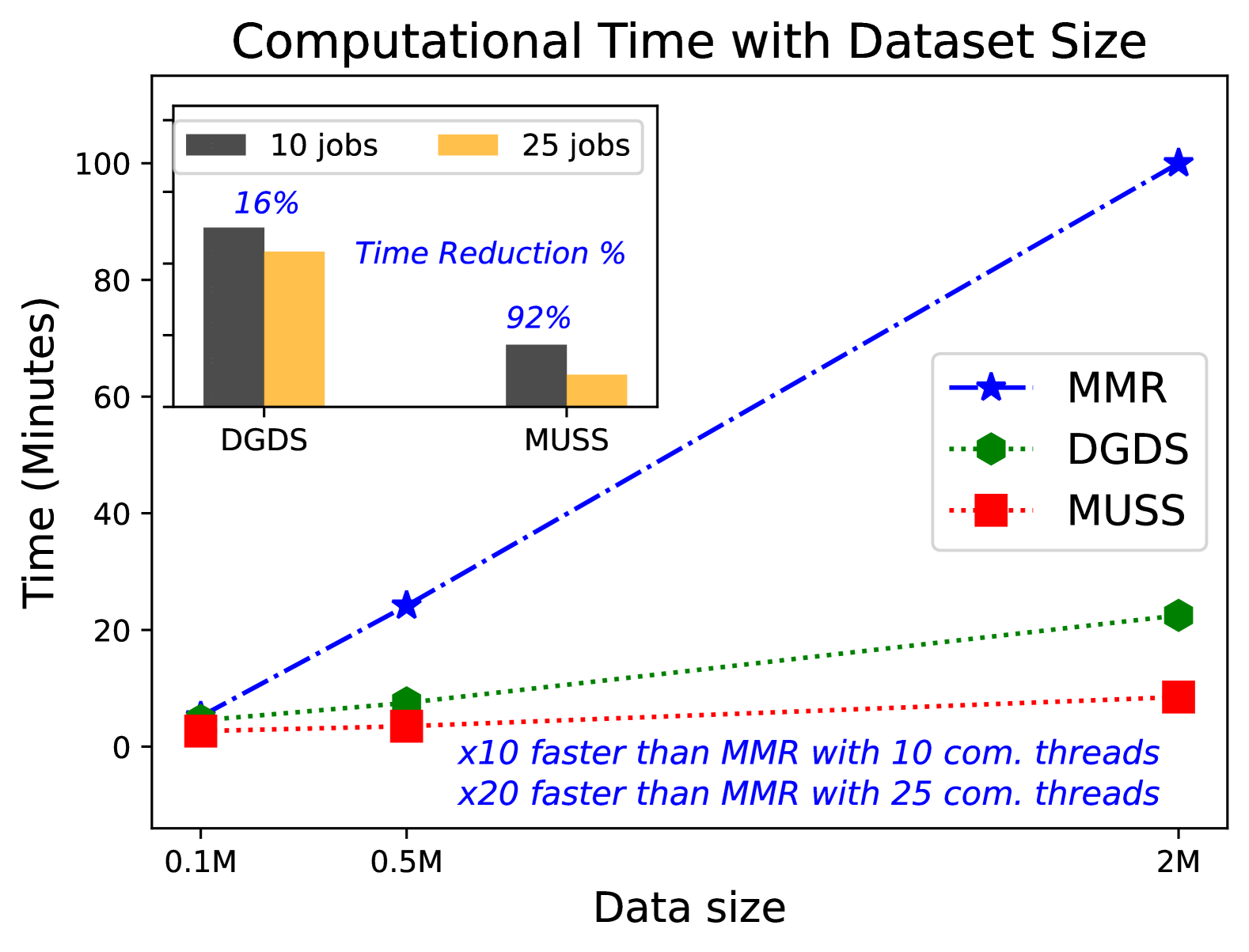
Figure 1: Our muss is capable of achieving the same level of performance on the target task as baselines, but up to $10\times$ faster when using $10$ computational threads. muss can be $4.5\times$ to $20\times$ faster than baselines, by further increasing the number of threads (insert shows times for the 2M dataset). Note that mmr is not a distributed method. Here, the task has been to select candidate items for recommendation from catalogs of different sizes.

2 Related Work

2.1 Relevant and Diverse Selection

Given the importance of the problem, there has been a number of approaches proposed in the literature.

Determinantal Point Process (DPP) is a probabilistic model that selects diverse subsets by maximizing the determinant of a kernel matrix representing item similarities (Kulesza et al., 2012). DPPs are effective in summarization, recommendation, and clustering tasks (Wilhelm et al., 2018; Elfeki et al., 2019; Yuan and Kitani, 2020; Nguyen et al., 2021). As discussed in reference (Li et al., 2016; Derezinski et al., 2019), the computational complexity of k-DPP can be $\mathcal{O}(k^{2}n+k^{3})$. Next, clustering-based methods ensure that different “regions” of the dataset are covered by the selection. Such methods cluster items (e.g., documents or features) and then select representatives from each cluster (Baeza-Yates, 2005; Wang et al., 2021; Panteli and Boutsinas, 2023; Ge et al., 2024). This approach is commonly used in text and image summarization. We use clustering in our method, but we depart from previous work in many other aspects (e.g., how we select within clusters, pruning clusters, theoretical analysis).

Reinforcement learning (RL) frameworks can be used to optimize diversity and relevance in sequential tasks such as recommendation and active learning. However, achieving an optimal balance between exploring diverse solutions and exploiting high-quality ones can be challenging, often leading to suboptimal convergence or increased training time (Levine et al., 2020; Fontaine and Nikolaidis, 2021). Model-based methods use application-specific probabilistic models or properties of relevance, quality, and diversity (Gao and Zhang, 2024; Pickett et al., 2024; Hirata et al., 2022; Acharya et al., 2024).

Maximum Marginal Relevance (mmr) is one of the most popular approaches for balancing relevance and diversity (Carbonell and Goldstein, 1998). Effectiveness of mmr has been demonstrated in numerous studies (Erkan and Radev, 2004; Wan and Yang, 2008; Xia et al., 2015). The algorithm was introduced in the context of retrieving similar but non-redundant documents for a given query $q$. Let ${\mathcal{U}}$ denote document corpus and ${\mathcal{S}}$ denote items selected so far. In each iteration, mmr evaluates all remaining candidates and selects item $s\in{\mathcal{U}}\setminus{\mathcal{S}}$ that maximizes criterion:

$$\text{MMR}(s)=\lambda\cdot\text{Sim}(s,q)-(1-\lambda)\cdot\max_{t\in{\mathcal{S}}}\text{Sim}(s,t),$$

where $\text{Sim}(.,.)$ measures similarity between two items, and $\lambda$ controls the trade-off between relevance and diversity.

2.2 Distributed Greedy Selection

The problem of subset selection can be viewed as maximization of a set-valued objective that assigns high values to subsets with desired properties (e.g., relevance of elements). Submodular functions is a special class of such objectives that has attracted significant attention. In particular, for a non-negative, monotone submodular function $f:2^{{\mathcal{U}}}\rightarrow\mathbb{R}$ and a cardinality constraint $k$, the solution ${\mathcal{S}}_{g}$ obtained by the greedy algorithm satisfies: $f({\mathcal{S}}_{g})\geq\left(1-\frac{1}{e}\right)f({\mathcal{S}}^{*})$ where ${\mathcal{S}}^{*}$ is the optimal solution of size at most $k$ (Nemhauser et al., 1978).

Distributed submodular maximization is an approach to solve submodular optimization problems in a distributed manner, e.g., when the dataset is too large to handle on a single machine (Mirzasoleiman et al., 2016; Barbosa et al., 2015). The authors provide theoretical analysis showing that under certain conditions one can achieve performance close to the non-distributed approach.

Since the addition of the diversity requirement results in a non-submodular objective for relevant and diverse selection, researchers had to relax the requirement for submodularity.

Beyond submodular maximization Ghadiri and Schmidt consider distributed maximization of so-called “submodular plus diversity” functions (Ghadiri and Schmidt, 2019). The authors introduce a framework, called dgds, for multi-label feature selection that balances relevance and diversity in the context of large-scale datasets. Their work addresses computational challenges posed by traditional submodular maximization techniques when applied to high-dimensional data. The authors propose a distributed greedy algorithm that leverages the additive structure of submodular plus diversity functions. This framework enables the decomposition of the optimization problem across multiple computational nodes, significantly reducing running time while preserving effectiveness.

However, items selected from different partitions are ultimately combined to perform the final selection step. Selecting objects in each partition, along with the final selection step becomes a performance bottleneck. Therefore, we further improve scalability of distributed selection by exploiting natural clustering structure in the data (Table 1). Moreover, we complement our method with a novel theoretical analysis of clustering-based selection.

Table 1: muss reduces time complexity by only considering a subset of clusters. Here, we compare average-case time complexity of methods for selecting subsets of size $k$ from a set of $n$ items. We use $l$ to denote the number of clusters, $m$ for the number of selected clusters, and $p$ for the number of parallel cores. Typically $n\gg l\gg m$. Complexity of muss is discussed in Section 3.2. For dgds and muss partitioning and clustering steps can be performed once and are not considered here.

Method	Computational Complexity
k-dpp	$\mathcal{O}(k^{2}n+k^{3}$)
mmr	$\mathcal{O}(k^{2}n)$
dgds	$\mathcal{O}\left(\frac{k^{2}n}{p}+k^{2}(kl)\right)$
muss	$\mathcal{O}\left(m^{2}l+\frac{k^{2}nm}{lp}+k^{2}(km)\right)$

3 muss: Multilevel Subset Selection

3.1 Problem Formulation

Consider a universe of objects represented as set ${\mathcal{U}}$ of size $|{\mathcal{U}}|=n$. Let $q:{\mathcal{U}}\rightarrow\mathbb{R}^{+}$ denote a non-negative function representing either quality of an object, relevance of the object, or a combination of both. Next, consider a distance function $d:{\mathcal{U}}\times{\mathcal{U}}\rightarrow\mathbb{R}^{+}$. Here we implicitly assume that the objects can be represented with embeddings in a metric space. Appendix Table 5 summarizes our notation.

Our goal is to select a subset ${\mathcal{S}}\subseteq{\mathcal{U}}$ of size $|{\mathcal{S}}|=k\leq n$ from the universe ${\mathcal{U}}$, such that the objects are both of high quality and diverse. In particular, we consider the following optimization problem

$${\mathcal{O}}=\arg\max_{{\mathcal{S}}\subseteq{\mathcal{U}},|{\mathcal{S}}|=k}F({\mathcal{S}}\mid k,\lambda)$$ (1)

where ${\mathcal{O}}$ is the global optimum, and the objective function is defined as

$$F({\mathcal{S}}\mid k,\lambda)= \lambda\sum_{{\bm{u}}\in{\mathcal{S}}}q({\bm{u}})+(1-\lambda)\sum_{{\bm{u}}\in{\mathcal{S}}}\sum_{{\bm{v}}\in{\mathcal{S}},{\bm{v}}\not={\bm{u}}}d({\bm{u}},{\bm{v}})$$

$$= \lambda Q({\mathcal{S}})+(1-\lambda)D({\mathcal{S}})$$ (2)

The first term $Q$ measures the quality of selection, while the second term $D$ measures the diversity of the selection. Coefficient $0\geq\lambda\geq 1$ controls the trade-off between quality (or relevance) and diversity. A higher value of $\lambda$ increases the emphasis on quality, while a lower value emphasizes diversity thus reducing redundancy. We use ${\mathcal{O}}$ to denote the global maximizer of the above problem parameterized by $k$ and $\lambda$. For brevity, we may omit $k$ and $\lambda$ throughout the paper and write $F({\mathcal{S}})$.

Note that the entire objective can be multiplied by a positive constant without changing the optimal solution. As such, different scaled variations of the diversity term can be represented with the same objective. For example, one can consider using an average distance for diversity, and this would lead to the same optimization problem with a different choice of $\lambda$.

The optimization involves maximizing a submodular function with a cardinality constraint, which is a well-known NP-hard problem. Therefore, our solution uses a greedy selection strategy similar to mmr. However, a direct application of mmr might not be practical for large sets. Distributed approach of dgds partially addresses this problem, but it still has a bottleneck in the final selection from the union of points selected from partitions.

3.2 Multilevel Selection

We address this bottleneck by considerably reducing the size of this union without compromising quality of selection. To this end, we propose muss, a method that performs selection in three stages: (i) selecting clusters, (ii) selecting objects within each selected cluster, and (iii) selecting the final set from the union of objects selected from the clusters (Figure 2). We show that muss achieves a constant factor approximation of the optimal solution.

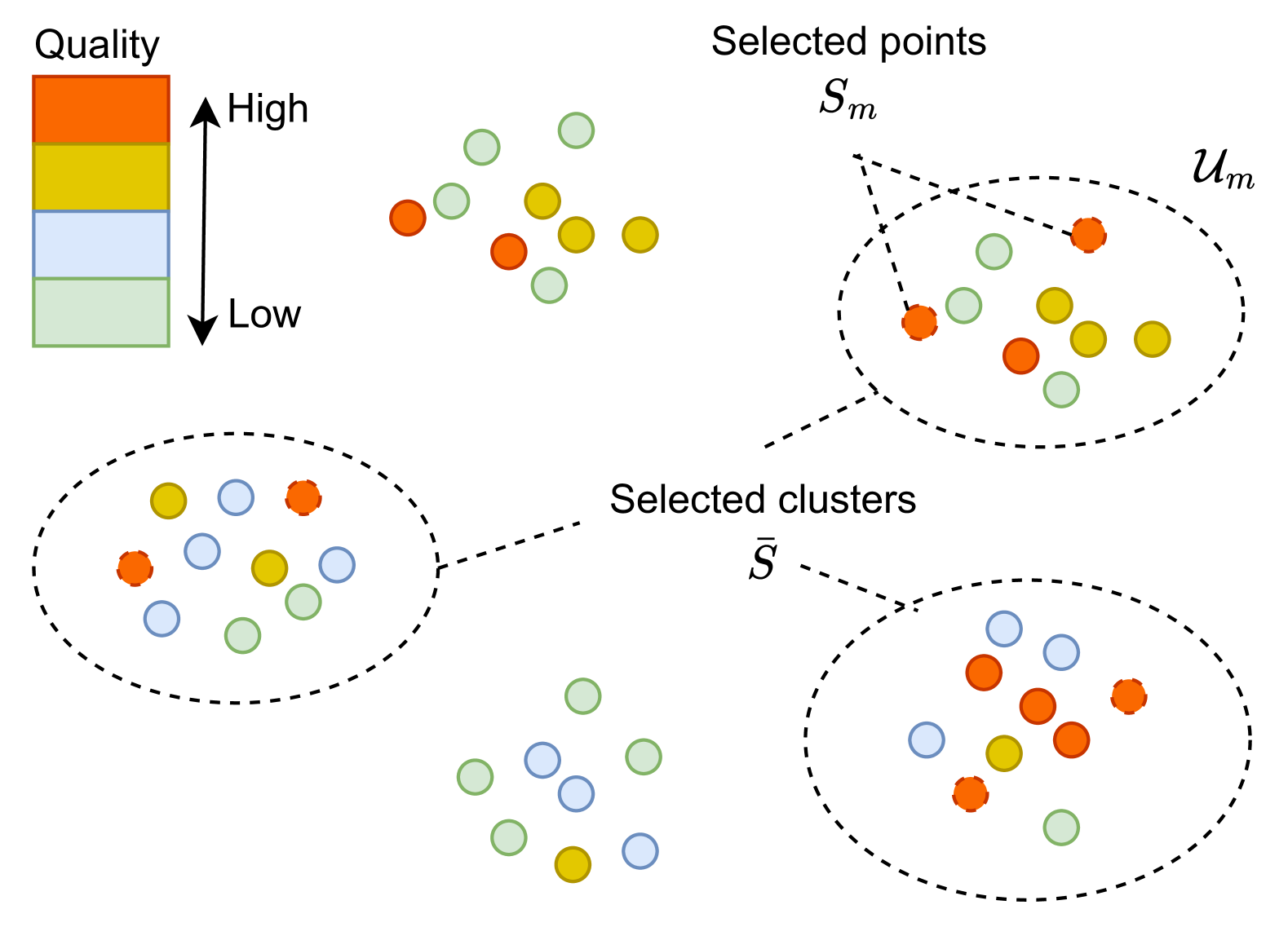
Figure 2: muss performs clustering following by a multilevel selection. Here, $\bar{{\mathcal{S}}}$ is a set of selected clusters, ${\mathcal{U}}_{m}$ denotes cluster $m$, and ${\mathcal{S}}_{m}$ denotes items selected from that cluster.

Step 1: While in previous literature greedy selection has been applied to items, our key observation is that greedy selection can also be used to select entire clusters that are both diverse and of high-quality while filtering out other clusters thus reducing the total pool of candidate items.

Therefore, we can use Kmeans algorithm to partition the data into clusters ${\mathcal{U}}=\bigcup_{i=1}^{l}{\mathcal{U}}_{i}$. Other clustering algorithms could also be used at this step. Next, we view clusters as a set of items ${\mathcal{C}}=\{c_{1},\ldots,c_{l}\}$. The distance $d(c_{i},c_{j})$ between two clusters is defined as the distance between cluster centroids. Next, the quality of the cluster is defined as the median quality score of items in this cluster, i.e., $q(c_{i})=\text{median}(\{q(a):a\in{\mathcal{U}}_{i}\})$. We then apply Algorithm 1 with the set of clusters ${\mathcal{C}}$ as input.

Algorithm 1 Greedy Selection

Input: set ${\mathcal{T}}$, number of items to select $k$, weights $w_{q},w_{d}$ Output: set ${\mathcal{S}}\subseteq{\mathcal{T}}$, s.t. $|{\mathcal{S}}|=k$

// start with the highest quality item

${\mathcal{S}}=\{\arg\max_{{\bm{t}}\in{\mathcal{T}}}q({\bm{t}})\}$

for $i=2,\ldots,k$ do

2    ${\bm{s}}=\arg\max_{{\bm{t}}\in{\mathcal{T}}\setminus{\mathcal{S}}}\left(w_{q}q({\bm{t}})+w_{d}\sum_{{\bm{u}}\in{\mathcal{S}}}d({\bm{t}},{\bm{u}})\right)$ ${\mathcal{S}}={\mathcal{S}}\cup\{{\bm{s}}\}$

Step 2: Using greedy selection at the cluster level will result in a subset of $m$ selected clusters, where each cluster $c_{i}$ contains items ${\mathcal{U}}_{i}\subset{\mathcal{U}}$. For each selected cluster, we independently apply Algorithm 1 to select ${\mathcal{S}}_{i}=\textsc{alg}1\bigl{(}{\mathcal{U}}_{i}|k,\lambda,(1-\lambda)\bigr{)}$ where $|{\mathcal{S}}_{i}|=k$. Importantly, selections within different clusters can be executed in parallel.

Step 3: We then select the final set of items by applying Algorithm 1 on the union of item sets obtained in the previous step. That is, our final selection is ${\mathcal{S}}=\textsc{alg}1\left(\cup_{i=1}^{m}{\mathcal{S}}_{i}|k,{\color[rgb]{1,.5,0}\frac{\lambda}{2}},(1-\lambda)\right)$ where $|{\mathcal{S}}|=k$.

The entire approach is summarized in Algorithm 2. In the last line, $\lambda$ is divided by $2$ for technical reasons to enable Eq. (7). However, this modification does not change the logic of our method, and can be simply viewed as using different weighting between relevance and diversity.

Algorithm 2 muss

Input: set ${\mathcal{U}}$; item-level parameters: number of items to select $k$, trade-off $\lambda$; cluster-level parameters: number of clusters $l$, number of clusters to select $m$, trade-off $\lambda_{c}$

Output: ${\mathcal{S}}\subseteq{\mathcal{U}}$ with $|{\mathcal{S}}|=k$

Apply $\textsc{Kmeans}{}({\mathcal{U}},l)$ to cluster ${\mathcal{U}}$ into $\{{\mathcal{U}}_{i}\}_{i=1}^{l}$

Let ${\mathcal{C}}$ denote a set of clusters. The distance between clusters and the quality of clusters are defined in Section 3.2.

$\bar{{\mathcal{S}}}=\textsc{alg}1\bigl{(}{\mathcal{C}}|m,\lambda_{c},(1-\lambda_{c})\bigr{)}$

for ${\mathcal{U}}_{i}\in\bar{{\mathcal{S}}}$ do

5   4 // selection within in each cluster ${\mathcal{S}}_{i}=\textsc{alg}1\bigl{(}{\mathcal{U}}_{i}|k,\lambda,(1-\lambda)\bigr{)}$

5// refinement to obtain final selection // division by 2 is needed for Eq. (7) ${\mathcal{S}}=\textsc{alg}1\left(\cup_{i=1}^{m}{\mathcal{S}}_{i}|k,{\color[rgb]{1,.5,0}\frac{\lambda}{2}},(1-\lambda)\right)$

Computational complexity: We discuss the average-case time complexity of muss. The complexity of standard iterative implementation of Kmeans algorithm (Lloyd, 1982) is $\mathcal{O}(nkt)$, where $t$ is the number of iterations. Greedy selection of $k$ out of $n$ items can be performed in $\mathcal{O}(k^{2}n)$ time. Therefore, selecting $m$ out of $l$ clusters results in $\mathcal{O}(m^{2}l)$. Next, selection of $k$ points within one cluster gives $\mathcal{O}(\frac{k^{2}n}{l})$ where the expected number of data points in each cluster is $\frac{n}{l}$. This will only be performed for $m$ selected clusters and the computation can be distributed across $p$ cores resulting in $\mathcal{O}(\frac{k^{2}nm}{lp})$. Combining subsets from the clusters results in a pool of $km$ items. Thus the final selection step results in $\mathcal{O}\bigl{(}k^{2}(km)\bigr{)}$ complexity. Clustering can be performed once. Thus at query time, average-case complexity is $\mathcal{O}\left(m^{2}l+\frac{k^{2}nm}{lp}+k^{2}(km)\right)$. Since our approach does not train a separate model for data selection, it does not require extra space. Therefore, the memory complexity is linear in the data size.

3.3 Theoretical Properties

We now present theoretical analysis of the proposed algorithm. We show that muss achieves a constant factor approximation of the optimal solution. Our main result is Theorem 6 which uses Lemmas 4 and 5 to bound, respectively, diversity and quality terms. Since muss uses both cluster and object-level selection, our bounds rely on Lemma 3 that relates objectives at different levels, and is one of our main innovation points. We also use auxiliary Lemmas 2 and 1. All proofs are provided in Appendix A.

Lemma 1.

The quality function $Q({\mathcal{S}})$ is non-negative, monotone and submodular.

Lemma 2.

Apply Algorithm 1 to select ${\mathcal{S}}=\textsc{alg}1({\mathcal{T}}|k,\lambda,(1-\lambda))$. Let $k>10$ and ${\bm{t}}\in{\mathcal{T}}\setminus{\mathcal{S}}$. The following inequalities hold

$$\Delta({\bm{t}},{\mathcal{S}})\equiv Q({\mathcal{S}}\cup\{{\bm{t}}\})-Q({\mathcal{S}})\leq\frac{5}{k\lambda}F({\mathcal{S}})$$ (3)

$$\min_{{\bm{z}}\in{\mathcal{S}}}d\bigl{(}{\bm{t}},{\bm{z}}\bigr{)}\leq\frac{4.5}{k(k-1)(1-\lambda)}F({\mathcal{S}})$$ (4)

After clustering, we can view clusters as artificial objects ${\mathcal{C}}=\{c_{1},\ldots,c_{l}\}$, where cluster “embeddings” are their centroids $\mu_{1},\ldots,\mu_{l}$. Let ${\mathcal{U}}_{i}\subseteq{\mathcal{U}}$ denote objects that belong to cluster $i$. We define the quality of each cluster as $q(c_{i})\equiv\text{median}(\{q({\bm{u}}):{\bm{u}}\in{\mathcal{U}}_{i}\})$.

Next, we use $r$ to denote the maximum radius among the clusters, i.e., the maximum distance between cluster centroid and the furthest point from centroid in that cluster. Similarly, we use $r_{q}$ to denote the maximum “quality radius”, i.e., $r_{q}\equiv\max_{i=1,...,l}\max_{{\bm{t}}\in{\mathcal{U}}_{i}}|q({\bm{t}})-q(c_{i})|$.

Using $\textsc{opt}(.)$ to denote the optimal selection that maximizes the objective $F$, we proceed to the following lemma.

Lemma 3.

When $k\geq m$, we have the inequality that

$$F\Bigl{(}\textsc{alg}1\bigl{(}{\mathcal{C}}|m,\lambda_{c},(1-\lambda_{c})\bigr{)}\Bigr{)}\leq$$

$$F\Bigl{(}\textsc{opt}(\cup_{i=1}^{m}{\mathcal{S}}_{i})|k\Bigr{)}+rm(m-1).$$ (5)

Lemma 3 connects objective functions at the cluster level and at the item level. In turn, this allows us to obtain lower bounds on the diversity term and the quality term when the multilevel Algorithm 2 is used to select ${\mathcal{S}}=\textsc{alg}2({\mathcal{U}})$.

Lemma 4.

If $m>10$ and $k\geq m$, we have

$$D({\mathcal{O}})\leq rk(k-1)\left[4+\frac{9m}{1-\lambda_{c}}\right]$$

$$+F\bigl{(}\textsc{opt}(\cup_{i=1}^{m}{\mathcal{S}}_{i})\bigr{)}\left[\frac{9k(k-1)}{(1-\lambda_{c})m(m-1)}+\frac{1}{(1-\lambda)}\right].$$ (6)

Lemma 5.

When $k\geq m>10$, we have

$Q({\mathcal{O}})\leq F\Bigl{(}\textsc{opt}(\cup_{i=1}^{m}{\mathcal{S}}_{i})\Bigr{)}\Bigl{[}\frac{6}{\lambda}+\frac{5k}{m\lambda_{c}}\Bigr{]}+\frac{5kr(m-1)}{\lambda_{c}}+kr_{q}$

Finally, our main theoretical result follows.

Theorem 6.

When $k\geq m>10$, muss  gives a constant-factor approximation to the optimal solution for maximizing $F({\mathcal{S}})$ s.t. $|{\mathcal{S}}|=k$.

$$F\bigl{(}\textsc{alg}2({\mathcal{U}})\bigr{)}\geq\frac{1}{\alpha}\Bigl{(}F({\mathcal{O}})-k\left(\beta r+\lambda r_{q}\right)\Bigr{)}.$$ (7)

Here, $\alpha(k,m,\lambda,\lambda_{c})$ and $\beta(k,m,\lambda,\lambda_{c})$ are intermediate quantities defined in the proof in the interest of space.

3.4 Discussion

Theoretical considerations.

In the above theorem, intermediate quantities $\alpha$ and $\beta$ are functions of algorithm parameters $k$, $m$, $\lambda$, $\lambda_{c}$. For fixed parameter values, $\alpha$ and $\beta$ are positive constants. We see that the bound improves as $r$ and $r_{q}$ get smaller.

Growing the number of clusters $l$ will make these radii smaller, but will increase time required for selecting clusters (Table 1). The ideal case is when the data naturally forms a small number of clusters, such that $l$, $r$, and $r_{q}$ are all low. Indeed, while in this work we have been using clustering based on object embeddings, we also identify clustering based on both relevance and diversity as a promising direction (Appendix B).

Next, the bound can be explicitly maximized as a function of $m$ and $\lambda_{c}$, although in practice, we simply evaluate results for different values of $\lambda_{c}$, while $m$ is selected to balance objective value with computational time.

Lastly, note that parameters $k$ and $\lambda$ are included in the objective function (Eq. 2). However, these parameters are application-driven, and should not be used to “optimize” the approximation bound. E.g., for a given application, the best $\lambda$ value is the one that results in strongest correlation between an application-specific performance metric and the objective $F$.

Practical considerations. One of the benefits of the proposed approach is that clustering can be performed in advance at a preprocessing stage. Each time a selection is required, a pre-existing clustering structure is leveraged. For large datasets, one can use scalable clustering methods, such as MiniBatchKmeans (Sculley, 2010) or FAISS (Douze et al., 2024). If new data arrives, an online clustering update can be used. In a simple case, one can store pre-computed cluster centroids and assign each newly arriving point to the nearest center.

In practice, we use the same parameters $k$, $w_{q}=\lambda$, and $w_{d}=(1-\lambda)$ when selecting items either within clusters (Line 5 of Algorithm 2) or from the union of selections (Line 6 of Algorithm 2). However, our method is flexible, and one can consider different $\lambda$ values for these selection stages. Finally, during the greedy selection, we normalize the sum of distances by the current selection size $|{\mathcal{S}}|$.

Benefits of cluster selection. Since item selection within clusters can be performed in parallel, the main performance bottleneck is item selection from the union of subsets derived from different clusters. In order to reduce the size of this union, we introduce a novel idea of relevant and diverse selection of clusters. This step can dramatically reduce the number of items at the final selection with minimum impact on the selection quality. To the best of our knowledge, previous approaches did not consider the idea of “pruning” the set of clusters.

Preliminary elimination of a large number of clusters (Line 3 of Algorithm 2) will not only allow for more efficient selection from the union of points (running time and memory for Line 6 of Algorithm 2), but can lead to improved accuracy. This is because the greedy algorithm will be able to focus on relevant items after redundancy across clusters has been reduced. This is particularly useful for large scale dataset size, as shown in our experiments. Moreover, novel theoretical analysis, such as Lemma 3, allows us to relate cluster-level and item-level selection stages and derive an approximation bound for the proposed muss.

4 Experiments

Amazon2M ($|{\mathcal{U}}|=2M$, $\lambda=0.9$)
Method	$\lambda_{c}$	Precision $\uparrow$	Objective $\uparrow$	Time $\downarrow$
random		32.9	0.530	0.0
k-dpp		✗	✗	✗
clustering		33.3	0.952	21
mmr		48.5	0.970	5,953
dgds		48.5	0.970	1,348
muss (rand.A)		48.4	0.969	485
muss (rand.B)		48.4	0.967	482
muss	0.1	48.2	0.965	484
muss	0.3	48.5	0.968	507
muss	0.5	48.5	0.969	505
muss	0.7	48.5	0.969	509
muss	0.9	48.5	0.969	513

Table 2: Precision on the candidate retrieval task for $k=500$ items. ✗  indicates that the method did not complete after 12 hours. Results are reported for $\lambda$ that maximizes precision achieved by mmr. For any value of $\lambda_{c}$, our method achieves similar performance as baselines but 2.5 to 10 times faster (10 computational threads).

The goals of our experiments have been to (i) test whether the proposed muss can be useful in practical applications; (ii) understand the impact of different components of our method, and (iii) understand scalability and parameter sensitivity of the proposed approach. Item recommendation and retrieval-augmented generation are among the most prominent applications of our subset selection problem. In the next two sections, we consider these applications, and compare muss with a number of baselines.

Baselines. Specifically, we consider the following previous methods for the task of high quality and diverse subset selection: random selection, k-dpp (Kulesza and Taskar, 2011), clustering-based selection, mmr as per Algorithm 1, and the distributed selection method called dgds (Ghadiri and Schmidt, 2019). We do not consider RL baselines here because we focus on selection methods that are potentially scalable, and also can be easily incorporated within existing ML systems. RL-based selection approaches require setting up a feedback loop and defining rewards which might not be trivial in a given ML application.

Key differences between dgds and muss are that (i) we propose clustering rather than random partitioning, and (ii) we select a subset of clusters, rather than using all of them. To understand the impact of these differences, we introduce two additional variations of our method. First, in “muss (rand.A)”, we perform clustering, but pick $m$ clusters at random rather than using greedy selection. Second, in “muss (rand.B)”, we perform random partitioning instead of clustering, but otherwise follow our Algorithm 2. Additional experimental details are given in Appendix C.1.

Table 3: Accuracy of question answering over different knowledge bases given a fixed LLM, but varying methods for RAG selection. For each dataset, we show the number of entities and $\lambda$ values that maximize mmr accuracy. For muss (random) variation we use $\lambda_{c}$ that maximized performance of this method. Our method muss matches, and in many cases outperforms all baselines.

DevOps ($|{\mathcal{U}}|=4722$, $\lambda=0.5$)			OpenBookQA ($|{\mathcal{U}}|=1326$, $\lambda=0.7$)			StackExchange ($|{\mathcal{U}}|=1025$, $\lambda=0.5$)
Method	$\lambda_{c}$	Accuracy $\uparrow$	Method	$\lambda_{c}$	Accuracy $\uparrow$	Method	$\lambda_{c}$	Accuracy $\uparrow$
random		42	random		78	random		40
k-dpp		40	k-dpp		76	k-dpp		44
clustering		48	clustering		80	clustering		60
mmr		62	mmr		82	mmr		68
dgds		60	dgds		82	dgds		68
muss (rand.A)		52	muss (rand.A)		80	muss (rand.A)		60
muss (rand.B)		50	muss (rand.B)		80	muss (rand.B)		58
muss	0.1	50	muss	0.1	82	muss	0.1	72
muss	0.3	52	muss	0.3	82	muss	0.3	72
muss	0.5	62	muss	0.5	84	muss	0.5	74
muss	0.7	62	muss	0.7	84	muss	0.7	74
muss	0.9	62	muss	0.9	82	muss	0.9	70

4.1 Candidate Retrieval for Product Recommendation

Context. Modern recommender systems typically consist of two stages. First, candidate retrieval aims at efficiently identifying a subset of relevant items from a large catalog of items (El-Kishky et al., 2023; Rajput et al., 2023). This step narrows down the input space for the second, more expensive, ranking stage. Since the ranking will not even consider items missed by candidate retrieval, it is crucial for the candidate retrieval stage to maximize recall — ensuring that most relevant items are included in the retrieved subset — while maintaining computational efficiency.

Setup. We use four datasets with sizes ranging from 4K to 2M (Table 2 and Appendix Table 6). These internally collected datasets represent either individual product categories, or larger collections of items across categories. Each data point corresponds to a product available at an online shopping service. For each product, an external ML model predicts the likelihood of an item being clicked on. The model takes into account product attributes, embedding, and historical performance. Likelihood predictions are treated as product quality scores, while actual clicks data is used as binary labels. We select $k=500$ items from a given dataset. For a fixed $k$ recall is proportional to precision@k, and we evaluate selection performance using Precision@500. In the experiment, we use either our method or a baseline to perform selection given the same set of quality scores.

Results for the largest dataset are shown in Table 2, while other results are provided in Appendix Table 6. First, higher values of the objective from Eq. (2) generally indicate higher precision, which further justifies our problem formulation. Next, it is clear that random selection or naive clustering-based strategy are not effective for this task as all other methods significantly outperform these baselines. Here, we use $\lambda=0.9$ which maximizes precision resulted from using mmr. Even with this setting muss achieves the same precision across various $\lambda_{c}$ values (slightly lower precision at $\lambda_{c}=0.1$). Importantly, muss achieves this results $10\times$ faster than mmr and $2.5\times$ faster than dgds. Improved scalability can be observed on datasets of different sizes (Figure 1 and Appendix Figure 8).

4.2 Q&A using Retrieval-augmented Generation

Context. Recently, Large Language Models (LLM) have gained significant popularity as core methods for a range of applications, from question answering bots to code generation. Retrieval-augmented Generation (RAG) refers to a technique where information relevant to the task is retrieved from a knowledge base and added to the LLM’s prompt. Given the importance of RAG, we have also evaluated muss for RAG entries selection.

Setup. We consider the task of answering questions over a custom knowledge corpus, and we use three datasets of varying degrees of difficulty (Table 3). OpenBookQA contains questions over common scientific knowledge (Mihaylov et al., 2018). On the other hand, StackExchange and DevOps datasets represent more specialized knowledge. These datasets were derived, respectively, from an online technical question answering service, and from AWS Dev Ops troubleshooting pages (Guinet et al., 2024).

Each dataset consists of a knowledge corpus and a number of multiple choice questions. For a given question, we compute relevance to entities in the corpus, and then use different methods for selecting $k=3$ relevant and diverse entities to be added to LLM’s prompt. For a fixed LLM we vary selection methods, and report proportion of correct answers over $50$ questions.

In this section, we are interested in accuracy of the answers rather than timing. We assume that given a question, one can effectively narrow down relevant scope of knowledge and the response time might be dominated by the LLM call.

Table 4: Precision (for Home and Amazon100k) or Accuracy (other datasets) achieved by muss with different number of clusters $l$, number of selected clusters $m$, and fixed $\lambda=\lambda_{c}=0.7$.

$l$	$m$	Home	Amazon100k	$l$	$m$	DevOps	OpenBookQA	StackExchange
100	50	66	32	50	10	48	80	68
200	50	65	33	50	20	48	82	68
200	100	66	37	100	10	48	84	68
500	50	61	30	100	20	48	82	70
500	100	65	36	200	10	52	80	70
500	200	67	40	200	20	48	82	70

Results are presented in Table 3. In all cases, accuracy can be improved compared to random selection. Since the choice of $\lambda$ (item-level selection trade-off) is application-specific, for each dataset, we identified and used $\lambda$ that maximizes mmr performance. Maximum accuracy is achieved with an intermediate value of the parameter, i.e., both relevance and diversity are important. Random selection and k-dpp baselines essentially emphasize diversity over relevance and achieve the weakest performance.

We can see that our method is capable of outperforming baselines by up to $6$ percent points when $\lambda_{c}\geq 0.5$ (cluster-level selection trade-off). The gain is most prominent on StackExchange dataset, where method outperforms all baselines at any $\lambda_{c}$ value. While muss can outperform baselines on OpenBookQA dataset, this dataset is likely to be “too easy” for a language model as it is based on general knowledge and relatively straightforward questions. On the other hand, muss matches the best baseline on DevOps dataset. Since this dataset involves complex troubleshooting questions, RAG approach itself might stop being effective past certain performance level. We conclude that our approach can lead to significant gains as long as RAG itself continues to contribute to increased accuracy.

4.3 Ablations, Parameter Sensitivity, and Scalability

Ablation Study. Note that variations “muss (rand.A)”, and “muss (rand.B)” constitute ablations of our method. In the former, we select clusters at random instead of using cluster-level greedy selection. We observe that using greedy selection consistently improves performance. Next, in “muss (rand.B)”, we use random partitioning instead of clustering. Again, we consistently observe improved performance when clustering is applied, and the gains can be significant. We conclude that leveraging natural structure in data is important for this problem. This is consistent with observed patterns discussed in Appendix C.2.

Sensitivity w.r.t. $\lambda$ and $\lambda_{c}$. Table 2, Table 3, and Appendix Table 6 show performance at different levels of $\lambda_{c}$ (cluster-level trade-off). Overall, for any dataset, there is little variation in performance when $\lambda_{c}\geq 0.5$. We also study how the diversity term $D({\mathcal{S}})$, the quality term $Q({\mathcal{S}})$, and the objective function $F({\mathcal{S}})$ varies with $\lambda$ and $\lambda_{c}$ in Appendix C.3. Consistent with the previous observation, we find that for any fixed $\lambda$, the variation due to $\lambda_{c}$ is relatively small. Next, as expected, small values of $\lambda$ (item-level trade-off) favour $D({\mathcal{S}})$ while larger $\lambda$ promote $Q({\mathcal{S}})$. The optimal choice of this parameter is application-specific. A practical way of setting the value could be cross-validation at some fixed $\lambda_{c}\geq 0.5$.

Sensitivity w.r.t. number of clusters $l$ and number of selected clusters $m$. We consider broad ranges for these parameter values. For example, we scale $l$ by $4$ to $5$ times, and $m$ by $2$ to $4$ times (while keeping both $\lambda$s fixed). Despite broad parameter ranges, in most cases, performance differences between different settings are within 5 percent points (Table 4). Larger deviations are typically observed as settings become more extreme (e.g., number of clusters is becoming too little for a dataset with 100k items).

Scalability. Figure 1 demonstrates scalability of the proposed muss. Specifically, given the dataset of size $|{\mathcal{U}}|=2M$, our method is up to $20$ times faster than mmr achieving the same precision. Here, all methods use the same $\lambda=0.5$ and we fix the hyperparameters to some constant values ($m=100,c=200,\lambda_{c}=0.5$). Further analysis into scalability shows that compared to dgds, our approach leads to time savings both during selection within partitions and during the final selection from the union of items (Appendix C.4 and Appendix Figure 8).

5 Conclusion

We propose a novel method for distributed relevant and diverse subset selection. We complement our method with theoretical analysis that relates cluster- and item-level selection and enables us to derive an approximation bound. Our evaluation shows that the proposed muss can considerably outperform baselines both in terms of scalability and performance on the target application. The problem of relevant and diverse subset selection has a wide range of applications, e.g., recommender systems and retrieval-augmented generation (RAG). This problem is NP-hard, and popular approaches such as Maximum Marginal Relevance (mmr) are based on greedy selection. Later methods, such as dgds considered a distributed setting using random data partitioning. In contrast, in our work, we leverage clustering structure in the data. Future directions of our work include considering continuous relaxation of the subset selection problem.

6 Impact Statement

This paper presents work whose goal is to advance the field of Machine Learning. There are many potential societal consequences of our work, none of which we feel must be specifically highlighted here.

Appendix A Proofs of Lemmas and the Theorem

In this appendix, we present proofs of lemmas and the theorem that represents our main result. Throughout the proofs, we make a technical assumption that $\lambda\not=0$ and $\lambda\not=1$ to avoid zero denomination when dividing for $\lambda$ or $1-\lambda$. Key notation used throughout the paper is summarized in Appendix Table 5.

Table 5: Notation used throughout the paper.

Variable	Definition
${\bm{u}}_{i}=({\bm{x}}_{i},q_{i})$	an item that can be viewed as a pair (embedding ${\bm{x}}_{i}\in{\mathbb{R}}^{d}$, quality score $q_{i}\in{\mathbb{R}}^{+}$)
${\mathcal{U}}=\{{\bm{u}}_{i}\}_{i=1}^{n}$	universe of items, dataset of size $n$ from which we select items
${\mathcal{U}}_{1},\ldots,{\mathcal{U}}_{m},\ldots,{\mathcal{U}}_{l}$	partitioned data, i.e., $\cup_{i=1}^{l}{\mathcal{U}}_{i}={\mathcal{U}}$
$r,r_{q}$	maximum radii from an item to its centre in the feature and quality spaces
$p\in\mathbb{N}$	the number of CPUs or computational threads for parallel jobs
${\mathcal{S}}\subseteq{\mathcal{U}}$, $k$	a set of selected items; number of items to select, $|{\mathcal{S}}|=k$
${\mathcal{C}},l,m$	a set of clusters (partitions); # clusters; # clusters to be selected, $l\geq m$.
$0\leq\lambda,\lambda_{c}\leq 1$	trade-off parameters between quality and diversity at different selection levels
$\bar{{\mathcal{S}}}=\textsc{alg}1\bigl{(}{\mathcal{C}}|m,\lambda_{c},(1-\lambda_{c})\bigr{)}$	$m$ clusters selected from ${\mathcal{C}}$ using Algorithm 1
${\mathcal{S}}_{i}=\textsc{alg}1\bigl{(}{\mathcal{U}}_{i}|k,\lambda,(1-\lambda)\bigr{)}$	$k$ items selected from ${\mathcal{U}}_{i}$ using Algorithm 1
$Q({\mathcal{S}}),D({\mathcal{S}})$	quality and diversity of subset ${\mathcal{S}}$
$\Delta({\bm{t}},{\mathcal{S}})=Q({\mathcal{S}}\cup\{{\bm{t}}\})-Q({\mathcal{S}})$	gain in quality score of subset ${\mathcal{S}}$ resulted from adding ${\bm{t}}$ to this subset

A.1 Proof of Lemma 1

Proof.

Our quality function $Q({\mathcal{S}})=\sum_{{\bm{u}}\in{\mathcal{S}}}q({\bm{u}})$ is non-negative as the quality $q(.)\geq 0$. Due to the additive property, the function $Q({\mathcal{S}})$ is monotone, i.e., $Q({\mathcal{S}})\leq Q({\mathcal{T}})$ for any ${\mathcal{S}}\subseteq{\mathcal{T}}$.

To prove submodularity, consider ${\mathcal{A}}\subseteq{\mathcal{B}}\subseteq{\mathcal{U}}$ and an element ${\bm{z}}\in{\mathcal{U}}\backslash{\mathcal{B}}$. The marginal gain of adding ${\bm{z}}$ to ${\mathcal{A}}$ and ${\mathcal{B}}$ is, respectively, $G({\mathcal{A}}\cup\{{\bm{z}}\})-G({\mathcal{A}})=q({\bm{z}})$ and $G({\mathcal{B}}\cup\{{\bm{z}}\})-G({\mathcal{B}})=q({\bm{z}})$. Since both marginal gains are equal, we have $G({\mathcal{A}}\cup\{{\bm{z}}\})-G({\mathcal{A}})=G({\mathcal{B}}\cup\{{\bm{z}}\})-G({\mathcal{B}})$ which satisfies the submodularity condition (in fact, this is a case of modularity, a stronger property than submodularity). ∎

A.2 Proof of Lemma 2

Proof.

Let $\textsc{alg}1$ denote Algorithm 1. Given Lemma 1, $\textsc{alg}1$ is a special case of Algorithm 1 from  Ghadiri and Schmidt [2019]. Thus our proof follows, but is not identical to, Theorem 1 from Ghadiri and Schmidt [2019]. Below, we present the proof details for the sake of completeness.

For any ${\bm{z}}\in{\mathcal{U}}$ and ${\mathcal{S}}\subseteq{\mathcal{U}}$, let $\Delta({\bm{z}},{\mathcal{S}}):=Q({\mathcal{S}}\cup\{{\bm{z}}\})-Q({\mathcal{S}})$. Next, let ${\bm{z}}_{1},\ldots,{\bm{z}}_{k}$ denote items that the algorithm $\textsc{alg}1$ selected in the order of selection. Define ${\mathcal{S}}_{i}:=\{{\bm{z}}_{1},\ldots,{\bm{z}}_{i}\}$ and ${\mathcal{S}}_{0}:=\emptyset$. Finally, let ${\bm{t}}\in{\mathcal{T}}\backslash\textsc{alg}1\bigl{(}{\mathcal{T}}|k,\lambda,(1-\lambda)\bigr{)}$.

Due to the greedy selection mechanism, we have the following

$$\lambda\Delta({\bm{z}}_{1},{\mathcal{S}}_{0})\geq \lambda\Delta({\bm{t}},{\mathcal{S}}_{0})$$ (8)

$$\lambda\Delta({\bm{z}}_{2},{\mathcal{S}}_{1})+(1-\lambda)d({\bm{z}}_{2},{\bm{z}}_{1})\geq \lambda\Delta({\bm{t}},{\mathcal{S}}_{1})+(1-\lambda)d({\bm{t}},{\bm{z}}_{1})$$ (9)

$$\ldots$$

$$\lambda\Delta({\bm{z}}_{k},{\mathcal{S}}_{k-1})+(1-\lambda)\sum_{i=1}^{k-1}d({\bm{z}}_{k},{\bm{z}}_{i})\geq \lambda\Delta({\bm{t}},{\mathcal{S}}_{k-1})+(1-\lambda)\sum_{i=1}^{k-1}d({\bm{t}},{\bm{z}}_{i}).$$ (10)

Adding these inequalities together gives us

$$\lambda Q({\mathcal{S}}_{k})+\frac{(1-\lambda)}{2}D({\mathcal{S}}_{k})\geq (1-\lambda)\sum_{i=1}^{k-1}(k-i)d({\bm{t}},{\bm{z}}_{i})+\lambda\sum_{i=0}^{k-1}\Delta({\bm{t}},{\mathcal{S}}_{i}).$$ (11)

Since $(1-\lambda)D({\mathcal{S}}_{k})\geq\frac{(1-\lambda)}{2}D({\mathcal{S}}_{k})$, we have

$$\lambda Q({\mathcal{S}}_{k})+(1-\lambda)D({\mathcal{S}}_{k})\geq (1-\lambda)\sum_{i=1}^{k-1}(k-i)d({\bm{t}},{\bm{z}}_{i})+\lambda\sum_{i=0}^{k-1}\Delta({\bm{t}},{\mathcal{S}}_{i})$$ (12)

$$\geq (1-\lambda)\sum_{i=1}^{k-1}(k-i)d({\bm{t}},{\bm{z}}_{i})+\lambda k\Delta({\bm{t}},S_{k})$$ (13)

where the second inequality is due to submodularity of $Q$.

We now consider Claim 1 from Ghadiri and Schmidt [2019] (proof is provided within that reference)

$$\sum_{i=1}^{k-1}(k-1)d({\bm{t}},{\bm{z}}_{i})+\sum_{i=\lceil\frac{k}{2}\rceil+1}^{k}\sum_{j=1}^{i-\lfloor\frac{k}{2}\rfloor-1}d({\bm{z}}_{i},{\bm{z}}_{j})\geq\sum_{i=1}^{k}(\lceil\frac{k}{2}\rceil-1)d({\bm{t}},{\bm{z}}_{i}).$$ (14)

where $\lceil\rceil$ and $\lfloor\rfloor$ denotes the ceiling and floor functions, respectively. Using this claim we have

$$2\bigl{(}\lambda Q({\mathcal{S}}_{k})+(1-\lambda)D({\mathcal{S}}_{k})\bigr{)}\geq (1-\lambda)D({\mathcal{S}}_{k})+\lambda Q({\mathcal{S}}_{k})+\sum_{i=\lceil\frac{k}{2}\rceil+1}^{k}\sum_{j=1}^{i-\lfloor\frac{k}{2}\rfloor-1}d({\bm{z}}_{i},{\bm{z}}_{j})$$ (15)

$$\geq (1-\lambda)\sum_{i=1}^{k-1}(k-i)d({\bm{t}},{\bm{z}}_{i})+\lambda k\Delta({\bm{t}},S_{k})+\sum_{i=\lceil\frac{k}{2}\rceil+1}^{k}\sum_{j=1}^{i-\lfloor\frac{k}{2}\rfloor-1}d({\bm{z}}_{i},{\bm{z}}_{j})$$ (16)

$$\geq (1-\lambda)\sum_{i=1}^{k}(\lceil\frac{k}{2}\rceil-1)d({\bm{t}},{\bm{z}}_{i})+\lambda(\lceil\frac{k}{2}\rceil-1)\Delta({\bm{t}},S_{k}).$$ (17)

Next, we obtain

$$2\bigl{(}\lambda Q({\mathcal{S}}_{k})+(1-\lambda)D({\mathcal{S}}_{k})\bigr{)}\geq (1-\lambda)\sum_{i=1}^{k}(\lceil\frac{k}{2}\rceil-1)d({\bm{t}},{\bm{z}}_{i})+\lambda(\lceil\frac{k}{2}\rceil-1)\Delta({\bm{t}},S_{k})$$ (18)

$$\frac{2}{\lceil\frac{k}{2}\rceil-1}F({\mathcal{S}}_{k})\geq (1-\lambda)\sum_{i=1}^{k}d({\bm{t}},{\bm{z}}_{i})+\lambda\Delta({\bm{t}},S_{k}).$$ (19)

Note that for $k\geq 10$, $\frac{5}{k}\geq\frac{2}{\lceil\frac{k}{2}\rceil-1}$ and also $\frac{4.5}{k-1}\geq\frac{2}{\lceil\frac{k}{2}\rceil-1}$. Therefore, from Eq. (19) we get

$$\lambda\Delta({\bm{t}},{\mathcal{S}}_{k})\leq \frac{5}{k}F({\mathcal{S}}_{k})$$ (21)

$$(1-\lambda)\sum_{i=1}^{k}d({\bm{t}},{\bm{z}}_{i})\leq \frac{4.5}{k-1}F({\mathcal{S}}_{k}).$$ (22)

Finally, we have that

$$\frac{4.5}{k(k-1)}F({\mathcal{S}}_{k})\geq(1-\lambda)\frac{1}{k}\sum_{i=1}^{k}d({\bm{t}},{\bm{z}}_{i})\geq(1-\lambda)\min_{i=1,\ldots,k}d({\bm{t}},{\bm{z}}_{i}).$$ (23)

This is because the minimum of positive values is not greater than their average. This concludes the proof.

The same way as $\textsc{alg}1$ can be used for selection of both clusters and individual items, this Lemma applies at both cluster and individual item levels. ∎

A.3 Proof of Lemma 3

Proof.

Without loss of generality, suppose that $\textsc{alg}1({\mathcal{C}}|m,\lambda_{c},(1-\lambda_{c}))$ selected clusters $c_{1},\ldots,c_{m}$. For each cluster $i$, let ${\mathcal{U}}_{i}\subseteq{\mathcal{U}}$ denote objects that belong to that cluster, and let $s_{i}^{\ast}$ denote an object with the highest quality score in that cluster, i.e., $s_{i}^{\ast}=\arg\max_{s\in{\mathcal{U}}_{i}}q(s)$.

Next, let ${\mathcal{S}}_{i}$ denote objects selected from that cluster by the algorithm, i.e., ${\mathcal{S}}_{i}=\textsc{alg}1({\mathcal{U}}_{i}|k,\lambda,(1-\lambda))$. It is clear that $s_{i}^{\ast}\in{\mathcal{S}}_{i}$.

Because of the way we define quality score for the clusters, i.e., $q(c_{i})=\text{median}(\{q(a):a\in{\mathcal{U}}_{i}\})$, we have $q(c_{i})\leq q(s_{i}^{\ast})$.

We also have $d(s_{i}^{\ast},\mu_{i})\leq r$ due to the definition of the radius $r$ (cluster radius is the distance from cluster centroid to the furthest point in the cluster)). Therefore,

$$D\Bigl{(}\{\mu_{1},\ldots,\mu_{m}\}\Bigr{)}\leq D\Bigl{(}\{s_{1}^{\ast},\ldots,s_{m}^{\ast}\}\Bigr{)}+rm(m-1).$$ (24)

We have that

$$F\Bigl{(}\textsc{alg}({\mathcal{C}})|m\Bigr{)}=F\Bigl{(}\{c_{1},\ldots,c_{m}\}|m\Bigr{)}\leq F\Bigl{(}\{s_{1}^{\ast},\ldots,s_{m}^{\ast}\}|m\Bigr{)}+rm(m-1).$$ (25)

Suppose $\{s_{1}^{\ast},\ldots,s_{m}^{\ast}\}\subseteq\textsc{opt}(\cup_{i=1}^{m}{\mathcal{S}}_{i})$. Then, due to the nature of our objective function

$$F\Bigl{(}\{s_{1}^{\ast},\ldots,s_{m}^{\ast}\}|m\Bigr{)}\leq F\Bigl{(}\textsc{opt}(\cup_{i=1}^{m}{\mathcal{S}}_{i})|k\Bigr{)}.$$ (26)

Finally, suppose $\{s_{1}^{\ast},\ldots,s_{m}^{\ast}\}\not\subseteq\textsc{opt}(\cup_{i=1}^{m}{\mathcal{S}}_{i})$, and $k\geq m$. Then if $F\Bigl{(}\{s_{1}^{\ast},\ldots,s_{m}^{\ast}\}|m\Bigr{)}>F\Bigl{(}\textsc{opt}(\cup_{i=1}^{m}{\mathcal{S}}_{i})|k)\Bigr{)}$, we could have replaced $m$ arbitrary points in $\textsc{opt}(\cup_{i=1}^{m}{\mathcal{S}}_{i})$ to get a higher value of $F(.|k)$. This would contradict the definition of $\textsc{opt}(\cup_{i=1}^{m}{\mathcal{S}}_{i})$ being the optimal set. Thus, again, we have

$$F\Bigl{(}\{s_{1}^{\ast},\ldots,s_{m}^{\ast}\}|m\Bigr{)}\leq F\Bigl{(}\textsc{opt}(\cup_{i=1}^{m}{\mathcal{S}}_{i})|k\Bigr{)}.$$ (27)

Combining this inequality with Eq. (25) gives the statement of the Lemma. ∎

A.4 Proof of Lemma 4

Proof.

Our method clusters embeddings of objects in ${\mathcal{U}}$. Let ${\mathcal{C}}$ denote the set of clusters, and $\lambda_{c}$ denote the hyperparameter for cluster selection. We select clusters using $\textsc{alg}1\bigl{(}{\mathcal{C}}|m,\lambda_{c},(1-\lambda_{c})\bigr{)}$. We then select objects from each cluster, and finally select objects from the union of selections. We use $\lambda$ to denote the hyperparameter for objects selection.

Consider the union of points from selected clusters. The subset selected from this union that maximizes the objective is denoted as $\textsc{opt}(\cup_{i=1}^{m}{\mathcal{S}}_{i})$.

Next, let $\mu({\bm{u}})$ denote the centroid of the cluster ${\bm{u}}$ belongs to, and let $h_{\bm{u}}$ be an auxiliary function defined as follows. If the cluster of ${\bm{u}}$ is selected, $h_{\bm{u}}$ equals to the centroid of that cluster. If the cluster of ${\bm{u}}$ is not selected, $h_{\bm{u}}$ equals to the nearest centroid among the selected clusters. Finally, let $r$ denote the largest radius among the clusters.

With these definitions in mind, and recalling that $d(.,.)$ is a metric, we have

$$D({\mathcal{O}})= \sum_{{\bm{u}}\in{\mathcal{O}}}\sum_{{\bm{v}}\in{\mathcal{O}},{\bm{v}}\not={\bm{u}}}d({\bm{u}},{\bm{v}})$$ (28)

$$\leq \sum_{{\bm{u}}\in{\mathcal{O}}}\sum_{{\bm{v}}\in{\mathcal{O}},{\bm{v}}\not={\bm{u}}}\Bigl{(}2r+d\bigl{(}\mu({\bm{u}}),\mu({\bm{v}})\bigr{)}\Bigr{)}$$ (29)

$$= 2rk(k-1)+\sum_{{\bm{u}}\in{\mathcal{O}}}\sum_{{\bm{v}}\in{\mathcal{O}},v\not={\bm{u}}}d\bigl{(}\mu({\bm{u}}),\mu({\bm{v}})\bigr{)}$$ (30)

$$\leq 2rk(k-1)+\sum_{{\bm{u}}\in{\mathcal{O}}}\sum_{{\bm{v}}\in{\mathcal{O}},v\not={\bm{u}}}d\bigl{(}\mu({\bm{u}}),h_{\bm{u}}\bigr{)}+d\bigl{(}\mu({\bm{v}}),h_{\bm{v}}\bigr{)}+d\bigl{(}h_{\bm{u}},h_{\bm{v}}\bigr{)}.$$ (31)

We now bound the three summation terms separately.

If the cluster of ${\bm{u}}$ is selected, $h_{\bm{u}}$ equals to $\mu({\bm{u}})$ and we have $d(\mu({\bm{u}}),h_{\bm{u}})=0$. If the cluster of ${\bm{u}}$ is not selected, we use Lemma 2 to upper bound Eq. (32). In both cases, we have that

$$\sum_{{\bm{u}}\in{\mathcal{O}}}\sum_{{\bm{v}}\in{\mathcal{O}},{\bm{v}}\not={\bm{u}}}d\bigl{(}\mu({\bm{u}}),h_{\bm{u}}\bigr{)}\leq\frac{4.5k(k-1)}{(1-\lambda_{c})m(m-1)}F\Bigl{(}\textsc{alg}1{({\mathcal{C}})}\Bigr{)}.$$ (32)

Similarly, we have

$$\sum_{{\bm{u}}\in{\mathcal{O}}}\sum_{{\bm{v}}\in{\mathcal{O}},{\bm{v}}\not={\bm{u}}}d\bigl{(}\mu({\bm{v}}),h_{\bm{v}}\bigr{)}\leq\frac{4.5k(k-1)}{(1-\lambda_{c})m(m-1)}F\Bigl{(}\textsc{alg}1{({\mathcal{C}})}\Bigr{)}.$$ (33)

Finally, we bound the third summation term $\sum_{{\bm{u}}\in{\mathcal{O}}}\sum_{{\bm{v}}\in{\mathcal{O}},{\bm{v}}\not={\bm{u}}}d(h_{\bm{u}},h_{\bm{v}})$.

Let $i=1,\ldots,m$ index selected clusters in arbitrary order. Recall that ${\mathcal{S}}_{i}$ denotes objects selected from cluster $i$.

Now consider an auxiliary set ${\mathcal{S}}_{\text{aux}}$, such that $\lvert{\mathcal{S}}_{\text{aux}}\rvert=k$, ${\mathcal{S}}_{\text{aux}}\subseteq\cup_{i=1}^{m}{\mathcal{S}}_{i}$, and $\lvert{\mathcal{S}}_{\text{aux}}\cap{\mathcal{S}}_{i}\rvert>0$ for any $i$. In other words, ${\mathcal{S}}_{\text{aux}}$ contains at least one object from each selected cluster.

Due to the above definitions, for any $h_{{\bm{u}}}$ we know that (i) it is a centroid of a selected cluster, and (ii) we can find an object within that cluster that is included in ${\mathcal{S}}_{\text{aux}}$. Let ${\bm{u}}^{\prime}$ and ${\bm{v}}^{\prime}$ be such objects from clusters of $h_{\bm{u}}$ and $h_{\bm{v}}$, respectively.

We have that

$$\sum_{{\bm{u}}\in{\mathcal{O}}}\sum_{{\bm{v}}\in{\mathcal{O}},{\bm{v}}\not={\bm{u}}}d(h_{\bm{u}},h_{\bm{v}})\leq \sum_{{\bm{u}}\in{\mathcal{O}}}\sum_{{\bm{v}}\in{\mathcal{O}},{\bm{v}}\not={\bm{u}}}\bigl{[}d\bigl{(}{\bm{u}}^{\prime}(h_{\bm{u}}),{\bm{v}}^{\prime}(h_{\bm{v}})\bigr{)}+2r\bigr{]}$$ (34)

$$\leq 2rk(k-1)+\frac{1}{(1-\lambda)}F\Bigl{(}{\mathcal{S}}_{\text{aux}}|k\Bigr{)}$$ (35)

$$\leq 2rk(k-1)+\frac{1}{(1-\lambda)}F\Bigl{(}\textsc{opt}(\cup_{i=1}^{m}{\mathcal{S}}_{i})|k\Bigr{)}.$$ (36)

Combining the three summations in Eqs. (32,33,36) into Eq. (31), we get

$$D({\mathcal{O}})\leq 4rk(k-1)+\frac{9k(k-1)}{(1-\lambda_{c})m(m-1)}F\bigl{(}\textsc{alg}{({\mathcal{C}})}\bigr{)}+\frac{1}{(1-\lambda)}F\Bigl{(}\textsc{opt}(\cup_{i=1}^{m}{\mathcal{S}}_{i})|k\Bigr{)}$$ (37)

$$\leq 4rk(k-1)+\frac{9rmk(k-1)}{1-\lambda_{c}}+F\Bigl{(}\textsc{opt}(\cup_{i=1}^{m}{\mathcal{S}}_{i})|k\Bigr{)}\left[\frac{9k(k-1)}{(1-\lambda_{c})m(m-1)}+\frac{1}{(1-\lambda)}\right]$$ (38)

$$= rk(k-1)\left[4+\frac{9m}{1-\lambda_{c}}\right]+F\Bigl{(}\textsc{opt}(\cup_{i=1}^{m}{\mathcal{S}}_{i})\Bigr{)}\left[\frac{9k(k-1)}{(1-\lambda_{c})m(m-1)}+\frac{1}{(1-\lambda)}\right].$$ (39)

Here Eq. (38) makes use of Lemma 3. ∎

A.5 Proof of Lemma 5

Proof.

Let us denote $\Delta(q,{\mathcal{S}})=Q({\mathcal{S}}\cup\{q\})-Q({\mathcal{S}})$. Let $o_{1},\ldots,o_{k}$ be an ordering of elements of the optimal set ${\mathcal{O}}$. For ${\bm{z}}=o_{i}\in{\mathcal{O}}$ define $O_{{\bm{z}}}=\{o_{1},\ldots,o_{i}-1\}$ and ${\mathcal{O}}_{o_{1}}=\emptyset$. Finally, recall that ${\mathcal{U}}_{i}$ denotes a data partition, and ${\mathcal{S}}_{i}=\textsc{alg}1\bigl{(}{\mathcal{U}}_{i}|k,\lambda,(1-\lambda)\bigr{)}$.

We bound the quality term by decomposing the optimal set ${\mathcal{O}}$ into points being selected and points not being selected.

$$Q({\mathcal{O}})= Q\Bigl{(}{\mathcal{O}}\cap(\cup_{i=1}^{m}{\mathcal{S}}_{i})\Bigr{)}+\sum_{{\bm{z}}\in{\mathcal{O}}\backslash(\cup_{i=1}^{m}{\mathcal{S}}_{i})}\Delta\Bigl{(}{\bm{z}},{\mathcal{O}}_{{\bm{z}}}\cup\bigl{(}{\mathcal{O}}\cap(\cup_{i=1}^{m}{\mathcal{S}}_{i})\bigr{)}\Bigr{)}$$ (40)

$$\leq \frac{1}{\lambda}F\Bigl{(}\textsc{opt}(\cup_{i=1}^{m}{\mathcal{S}}_{i})\Bigr{)}+\sum_{{\bm{z}}\in{\mathcal{O}}\backslash(\cup_{i=1}^{m}{\mathcal{S}}_{i})}\Delta({\bm{z}},{\mathcal{O}}_{{\bm{z}}})$$ (41)

$$= \frac{1}{\lambda}F\Bigl{(}\textsc{opt}(\cup_{i=1}^{m}{\mathcal{S}}_{i})\Bigr{)}+\sum_{i=1}^{l}\sum_{{\bm{z}}\in{\mathcal{O}}\cap{\mathcal{U}}_{i}\backslash{\mathcal{S}}_{i}}\Delta({\bm{z}},{\mathcal{O}}_{{\bm{z}}}\cup{\mathcal{S}}_{i})+\Delta({\bm{z}},{\mathcal{O}}_{\bm{z}})-\Delta({\bm{z}},{\mathcal{O}}_{{\bm{z}}}\cup{\mathcal{S}}_{i})$$ (42)

$$\leq \frac{1}{\lambda}F\Bigl{(}\textsc{opt}(\cup_{i=1}^{m}{\mathcal{S}}_{i})\Bigr{)}+\sum_{i=1}^{m}\sum_{{\bm{z}}\in{\mathcal{O}}\cap{\mathcal{U}}_{i}\backslash{\mathcal{S}}_{i}}\Delta({\bm{z}},{\mathcal{S}}_{i})+\sum_{i=m+1}^{l}\sum_{{\bm{z}}\in{\mathcal{O}}\cap{\mathcal{U}}_{i}}\Delta({\bm{z}},\emptyset)$$ (43)

$$\leq \frac{1}{\lambda}F\Bigl{(}\textsc{opt}(\cup_{i=1}^{m}{\mathcal{S}}_{i})\Bigr{)}+\sum_{i=1}^{m}\sum_{{\bm{z}}\in{\mathcal{O}}\cap{\mathcal{U}}_{i}\backslash{\mathcal{S}}_{i}}\frac{5}{k\lambda}F({\mathcal{S}}_{i})+\sum_{i=m+1}^{l}\sum_{{\bm{z}}\in{\mathcal{O}}\cap{\mathcal{U}}_{i}}\Delta({\bm{z}},\emptyset).$$ (44)

In Eq. (43), we use the fact that $\Delta({\bm{z}},{\mathcal{O}}_{\bm{z}})-\Delta({\bm{z}},{\mathcal{O}}_{{\bm{z}}}\cup{\mathcal{S}}_{i})=Q({\bm{z}})-Q({\bm{z}})=0$ and $\Delta({\bm{z}},{\mathcal{O}}_{{\bm{z}}}\cup{\mathcal{S}}_{i})\leq\Delta({\bm{z}},{\mathcal{S}}_{i})$. In Eq. (44), we use Lemma 2.

Now let ${\mathcal{C}}=\{c_{1},\ldots,c_{l}\}$ denote the clusters. Recall that ${\mathcal{U}}_{i}$ denotes objects in cluster $i$, while the quality of cluster $i$ is defined as $q(c_{i})=\text{median}(\{q({\bm{t}}):{\bm{t}}\in{\mathcal{U}}_{i}\})$. Let us define the “radius” over the quality scores $r_{q}\equiv\max_{i=1,...,l}\max_{{\bm{t}}\in{\mathcal{U}}_{i}}|q({\bm{t}})-q(c_{i})|$. This “quality radius” is the largest gap between the quality of an object and the cluster the object belongs to. For example, if object ${\bm{z}}$ belongs to cluster $c_{{\bm{z}}}$ we have $\Delta({\bm{z}},\emptyset)=Q(\{{\bm{z}}\})\leq Q(\{c_{{\bm{z}}}\})+r_{q}$.

Without loss of generality, suppose that $\textsc{alg}1({\mathcal{C}})$ selects clusters $c_{1},\ldots,c_{m}$, and let $c_{{\bm{z}}}$ denote any unselected cluster. Lemma 2 applied at the cluster level gives $\Delta(c_{{\bm{z}}},\{c_{1},\ldots,c_{m}\})\leq\frac{5}{m\lambda_{c}}F\bigl{(}\textsc{alg}{({\mathcal{C}})}\bigr{)}$. By the definition of the quality function $Q(.)$ and since $c_{{\bm{z}}}$ is not in $\{c_{1},\ldots,c_{m}\}$ we have that $\Delta(c_{{\bm{z}}},\{c_{1},\ldots,c_{m}\})=Q(\{c_{{\bm{z}}}\})\leq\frac{5}{m\lambda_{c}}F\bigl{(}\textsc{alg}{({\mathcal{C}})}\bigr{)}$. With these facts in mind, we continue Eq. (44) as follows

$$Q({\mathcal{O}})\leq \frac{1}{\lambda}F\Bigl{(}\textsc{opt}(\cup_{i=1}^{m}{\mathcal{S}}_{i})\Bigr{)}+\sum_{i=1}^{m}\sum_{{\bm{z}}\in{\mathcal{O}}\cap{\mathcal{U}}_{i}\backslash{\mathcal{S}}_{i}}\frac{5}{k\lambda}F(S_{i})+\sum_{i=m+1}^{l}\sum_{{\bm{z}}\in{\mathcal{O}}\cap{\mathcal{U}}_{i}}\Bigl{[}Q(\{c_{{\bm{z}}}\})+r_{q}\Bigr{]}$$ (45)

$$\leq \frac{1}{\lambda}F\Bigl{(}\textsc{opt}(\cup_{i=1}^{m}{\mathcal{S}}_{i})\Bigr{)}+\sum_{i=1}^{m}\sum_{{\bm{z}}\in{\mathcal{O}}\cap{\mathcal{U}}_{i}\backslash{\mathcal{S}}_{i}}\frac{5}{k\lambda}F(S_{i})+\frac{5k}{m\lambda_{c}}F(\textsc{alg}{({\mathcal{C}})})+kr_{q}$$ (46)

$$\leq \frac{1}{\lambda}F\Bigl{(}\textsc{opt}(\cup_{i=1}^{m}{\mathcal{S}}_{i})\Bigr{)}+\sum_{i=1}^{m}\sum_{{\bm{z}}\in{\mathcal{O}}\cap{\mathcal{U}}_{i}\backslash{\mathcal{S}}_{i}}\frac{5}{k\lambda}F(S_{i})+\frac{5k}{m\lambda_{c}}\Bigl{[}F\Bigl{(}\textsc{opt}(\cup_{i=1}^{m}{\mathcal{S}}_{i})|k\Bigr{)}+rm(m-1)\Bigr{]}+kr_{q}$$ (47)

$$\leq \frac{1}{\lambda}F\Bigl{(}\textsc{opt}(\cup_{i=1}^{m}{\mathcal{S}}_{i})\Bigr{)}+\frac{5}{\lambda}F\Bigl{(}\textsc{opt}(\cup_{i=1}^{m}{\mathcal{S}}_{i})\Bigr{)}+\frac{5k}{m\lambda_{c}}\Bigl{[}F\Bigl{(}\textsc{opt}(\cup_{i=1}^{m}{\mathcal{S}}_{i})\Bigr{)}+rm(m-1)\Bigr{]}+kr_{q}$$ (48)

$$\leq F\Bigl{(}\textsc{opt}(\cup_{i=1}^{m}{\mathcal{S}}_{i})\Bigr{)}\Bigl{[}\frac{6}{\lambda}+\frac{5k}{m\lambda_{c}}\Bigr{]}+\frac{5kr(m-1)}{\lambda_{c}}+kr_{q}.$$ (49)

We have utilized Lemma 3 in Eq. (47). ∎

A.6 Proof of Theorem 6

Proof.

Using Lemma 5, we have $Q({\mathcal{O}})\leq F\Bigl{(}\textsc{opt}(\cup_{i=1}^{m}{\mathcal{S}}_{i})\Bigr{)}\Bigl{[}\frac{6}{\lambda}+\frac{5k}{m\lambda_{c}}\Bigr{]}+\frac{5kr(m-1)}{\lambda_{c}}+kr_{q}$.

Next, Lemma 4 gives $D({\mathcal{O}})\leq rk(k-1)\left[4+\frac{9m}{1-\lambda_{c}}\right]+F\Bigl{(}\textsc{opt}(\cup_{i=1}^{m}{\mathcal{S}}_{i})\Bigr{)}\left[\frac{9k(k-1)}{(1-\lambda_{c})m(m-1)}+\frac{1}{(1-\lambda)}\right]$.

Let $\frac{\alpha}{2}\equiv 9\frac{k(k-1)}{m(m-1)}\frac{(1-\lambda)}{(1-\lambda_{c})}+5\frac{k}{m}\frac{\lambda}{\lambda_{c}}+7$. We have that

$$F({\mathcal{O}})= \lambda Q({\mathcal{O}})+(1-\lambda)D({\mathcal{O}})$$ (50)

$$\leq \frac{\alpha}{2}F\bigl{(}\textsc{opt}(\cup_{i=1}^{m}{\mathcal{S}}_{i})\bigr{)}+rk\left[5(m-1)\frac{\lambda}{\lambda_{c}}+(k-1)(1-\lambda)\left[4+\frac{9m}{1-\lambda_{c}}\right]\right]+r_{q}k\lambda.$$ (51)

Now, let $\beta\equiv\left[5(m-1)\frac{\lambda}{\lambda_{c}}+(k-1)(1-\lambda)\left[4+\frac{9m}{1-\lambda_{c}}\right]\right]$.

In other words,

$$F\Bigl{(}\textsc{opt}(\cup_{i=1}^{m}{\mathcal{S}}_{i})\Bigr{)}\geq\frac{2}{\alpha}F({\mathcal{O}})-\frac{2\beta}{\alpha}rk-\frac{2}{\alpha}\lambda r_{q}k.$$ (52)

Following Ghadiri and Schmidt [2019] and Borodin et al. [2017] we have that the final greedy selection in Algorithm 2 is a half approximation for maximizing $F$, i.e.,

$$2F\Bigl{(}\textsc{alg}1\bigl{(}\cup_{i=1}^{m}{\mathcal{S}}_{i}\mid k,\frac{\lambda}{2},(1-\lambda)\bigr{)}\Bigr{)}\geq F\Bigl{(}\textsc{opt}(\cup_{i=1}^{m}{\mathcal{S}}_{i})\Bigr{)}.$$ (53)

We conclude that

$$F\bigl{(}\textsc{alg}2({\mathcal{U}})\bigr{)}\geq\frac{1}{\alpha}F({\mathcal{O}})-\frac{\beta}{\alpha}rk-\frac{\lambda}{\alpha}r_{q}k=\frac{1}{\alpha}\Bigl{(}F({\mathcal{O}})-k\left(\beta r+\lambda r_{q}\right)\Bigr{)}.$$ (54)

∎

Appendix B Kmeans Clustering in Both Feature and Quality Spaces

Consider a dataset of $n$ objects ${\mathcal{U}}=\{{\bm{u}}_{i}\}_{i=1}^{n}$, where each object is represented with a pair of embedding ${\bm{x}}_{i}\in{\mathbb{R}}^{d}$, and quality score $q_{i}\in{\mathbb{R}}^{+}$. With clustering we aim to partition the data into $\{{\mathcal{U}}_{j}\}_{j=1}^{l}$ clusters.

A clustering objective associated with Kmeans aims to minimize the sum of squared distances between each data point and the centroid of the cluster to which the point belongs. We can extend the original objective function [Lloyd, 1982] to include the quality score as follows:

$${\mathcal{L}}=\min_{{\bm{a}}}\sum_{j=1}^{l}\sum_{i=1}^{n}a_{ij}\Bigl{[}\underbrace{\|\mathbf{x}_{i}-\mathbf{{\bm{\mu}}}_{j}\|^{2}}_{\text{feature space}}+w_{c}\underbrace{\|q_{i}-\phi_{k}\|^{2}}_{\text{quality space}}\Bigr{]}$$ (55)

where

• $l$ is the number of clusters.

• $\mathbf{{\bm{\mu}}}_{1},\ldots,\mathbf{{\bm{\mu}}}_{l}$ are the mean values of embeddings of objects included in each cluster (cluster centroids).

• $\mathbf{\phi}_{1},\ldots,\mathbf{\phi}_{l}$ are the mean values of quality scores of objects included in each cluster (“quality centroids”).

• $a_{ij}$ is an indicator variable that equals 1 if an item $i$ is assigned to cluster $j$, and $0$ otherwise.

• $\|.\|^{2}$ is the Euclidean distance.

• $w_{c}$ is a weight representing trade-off between the two spaces.

B.1 Gradient of the Objective Function

The classical Kmeans algorithm minimizes the objective function using an iterative process, which can be viewed as gradient-based optimization. We can express the gradient of the objective with respect to the centroids as:

$$\frac{\partial{\mathcal{L}}}{\partial{\bm{\mu}}_{j}}=-2\sum_{\mathbf{x}\in{\mathcal{U}}_{j}}(\mathbf{x}-{\bm{\mu}}_{j})$$ (56)

$$\frac{\partial{\mathcal{L}}}{\partial\mathbf{\phi}_{j}}=-2\sum_{q\in{\mathcal{U}}_{j}}(q-\mathbf{\phi}_{j})$$ (57)

$$\frac{\partial{\mathcal{L}}}{\partial a_{ij}}=\underbrace{\|\mathbf{x}_{i}-\mathbf{{\bm{\mu}}}_{j}\|^{2}}_{\text{feature space}}+w_{c}\underbrace{\|q_{i}-\phi_{k}\|^{2}}_{\text{quality space}}.$$ (58)

B.2 Optimization Step

To update the centroids, we find the values that set the gradient to zero:

$${\bm{\mu}}_{j}=\frac{1}{|{\mathcal{U}}_{j}|}\sum_{\mathbf{x}\in{\mathcal{U}}_{j}}\mathbf{x}$$

$$\mathbf{\phi}_{k}=\frac{1}{|{\mathcal{U}}_{j}|}\sum_{q\in{\mathcal{U}}_{j}}q.$$

These represent means of all objects assigned to a cluster, which is why the algorithm is called the ”k-Means” algorithm. The centroids are updated iteratively until convergence, ensuring that the objective function is minimized.

Since $a_{ij}$ is binary, the assignment is:

$$a_{ij}=\begin{cases}1&\text{if }j=\arg\min_{1,\ldots,l}\|\mathbf{x}_{i}-\mathbf{{\bm{\mu}}}_{j}\|^{2}+w_{c}\|q_{i}-\phi_{j}\|^{2},\\ 0&\text{otherwise}.\end{cases}$$

The gradient indicates that $a_{ij}$ should be updated in a way that reduces the distance between object $i$ and cluster $j$.

In Appendix Section C.5, we present an empirical comparison of our muss method using the clustering with and without the quality space.

Appendix C Additional Experimental Details

C.1 Technical Details

The candidate retrieval task is performed using AWS instance ml.r5.16xlarge with 64 CPUs, $10$ computational threads and 512 GB RAM. For Figure 1, we also utilize another larger AWS instance ml.r5.24xlarge with 96 CPUs, $25$ computational threads and 512 GB RAM. The embedding dimension for candidate retrieval is $d=1024$.

For both candidate retrieval and question answering tasks, mmr performance was evaluated on $\lambda$ values in $\{0.1,0.3,0.5,0.7,0.9\}$.

For question answering task, we used anthropic.claude-instant-v1, with the idea that a smaller model complemented with RAG is a more cost-effective solution compared to using a much larger model. Also using a smaller model enabled us to see the effect of RAG more clearly. Next, prompt instructions included the following words: “You will be given a question and additional information to consider. This information might or might not be relevant to the question. Your task is to answer the question. Only use additional information if it’s relevant…. (RAG results) … (question) … In your response, only include the answer itself. No tags, no other words.”

For question and corpus embeddings, we used HuggingFaceEmbeddings.embed_documents() with default parameters. The embedding dimension is $d=768$. Number of questions for each dataset was $50$.

In the results, mmr denotes greedy selection as per Algorithm 1. We have also evaluated greedy selection using the original maximum similarity criterion. [Carbonell and Goldstein, 1998]. Overall the results are slightly worse compared to the sum-based criterion, see Appendix Section C.6.

C.2 Additional Results

Full results for candidate item selection are presented in Table 6. The proposed muss  consistently performs the best while significantly reduce the computational time. We note that while mmr will still find the highest objective function score since it directly maximizes Eq. (1), our muss  also achieves comparable objective scores across four datasets.

Moreover, we have performed tSNE Visualization [Van der Maaten and Hinton, 2008] for selecting $k=100$ items for “Home” and “Kitchen” datasets (Figure 3). We observe that the data forms coherent clusters. Our method tends to selects data points which are of high quality while being spread out within the space.

Kitchen ($|{\mathcal{U}}|=3872$, $\lambda=0.9$)
Method	$\lambda_{c}$	Precision $\uparrow$	Objective $\uparrow$	Quality $\uparrow$	Diversity $\uparrow$	Time $\downarrow$
random		50.0	0.687	0.693	0.638	0
k-dpp		46.4	0.749	0.762	0.636	5.88
clustering		61.6	0.879	0.906	0.641	0.59
mmr		83.6	0.959	0.998	0.625	12.1
dgds		83.6	0.959	0.998	0.625	12.18
muss(rand.A)		84.0	0.96	0.998	0.631	5.42
muss(rand.B)		83.6	0.96	0.998	0.632	7.01
muss	0.1	79.8	0.954	0.992	0.644	6.34
muss	0.3	84.4	0.959	0.997	0.636	7.54
muss	0.5	84.0	0.959	0.997	0.633	8.11
muss	0.7	83.8	0.960	0.997	0.622	8.30
muss	0.9	84.0	0.960	0.997	0.618	8.24

Home ($|{\mathcal{U}}|=4737$, $\lambda=0.9$)
Method	$\lambda_{c}$	Precision $\uparrow$	Objective $\uparrow$	Quality $\uparrow$	Diversity $\uparrow$	Time $\downarrow$
random		51.6	0.778	0.793	0.642	0.0
k-dpp		43.2	0.739	0.749	0.643	7.9
clustering		61.4	0.923	0.953	0.646	0.69
mmr		69.0	0.963	0.998	0.648	13.5
dgds		69.0	0.963	0.998	0.648	13.7
muss(rand.A)		59.7	0.847	0.937	0.638	6.7
muss(rand.B)		62.1	0.882	0.983	0.646	6.6
muss	0.1	64.2	0.960	0.997	0.643	7.12
muss	0.3	69.4	0.962	0.998	0.633	7.86
muss	0.5	69.0	0.962	0.998	0.634	8.91
muss	0.7	68.6	0.962	0.998	0.634	9.17
muss	0.9	69.2	0.962	0.998	0.636	8.18

Amazon100k ($|{\mathcal{U}}|=108,258$, $\lambda=0.9$)
Method	$\lambda_{c}$	Precision $\uparrow$	Objective $\uparrow$	Quality $\uparrow$	Diversity $\uparrow$	Time $\downarrow$
random		12.8	0.730	0.736	0.674	0.0
k-dpp		✗	✗	✗	✗	✗
clustering		28.2	0.963	0.995	0.677	9.92
mmr		36.4	0.970	0.999	0.711	311
dgds		36.4	0.970	0.999	0.711	271
muss(rand.A)		38.6	0.969	0.999	0.698	118
muss(rand.B)		35.4	0.969	0.999	0.700	125
muss	0.1	41.0	0.970	0.999	0.703	128
muss	0.3	42.4	0.970	0.999	0.705	145
muss	0.5	44.0	0.970	0.999	0.706	158
muss	0.7	44.4	0.970	0.999	0.706	166
muss	0.9	43.8	0.970	0.999	0.705	159

Table 6: Comparison on candidate retrieval to select $k=500$ items. ✗  denotes that the algorithm did not complete within 12 hours of running. We use hyperparameter $\lambda$ value that maximized the performance for the mmr baseline. Our method achieves competitive performance and is faster than mmr and dgds. Note that we focus on the Precision and Time as the main metrics for comparison while the other metrics are complementary. The highest precision score is in bold.

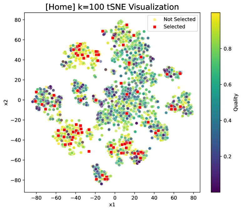
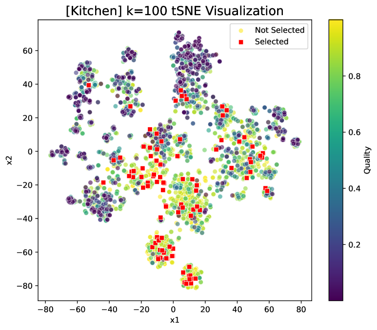
Figure 3: tSNE Visualization of selecting $k=100$ items for “Home” and “Kitchen” datasets. Data forms clusters. Our method performs high-quality and diverse selection as shown by the red dots. The color scale indicates the quality score of the item.

C.3 Varying $\lambda$ and $\lambda_{c}$

In this study, we varied the trade-off parameters $\lambda_{c}$ (cluster-level selection) and $\lambda$ (item-level selection). We report the values of quality term $Q({\mathcal{S}})$, diversity term $D({\mathcal{S}})$, and the overall objective function $F({\mathcal{S}})$ as defined in Eq. (1). Results are shown in Figures 4, 5, 6, and  7. As expected, when $\lambda$ increases, our objective function favours the quality term. Interestingly, for a fixed $\lambda$, the objective remains relatively stable at all values of $\lambda_{c}$.

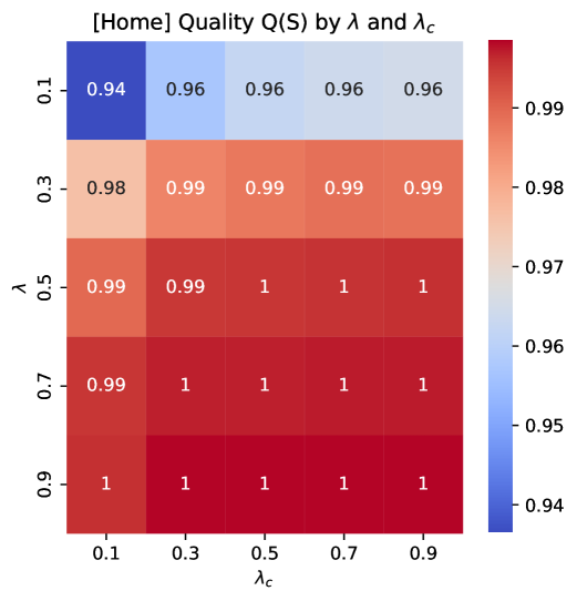
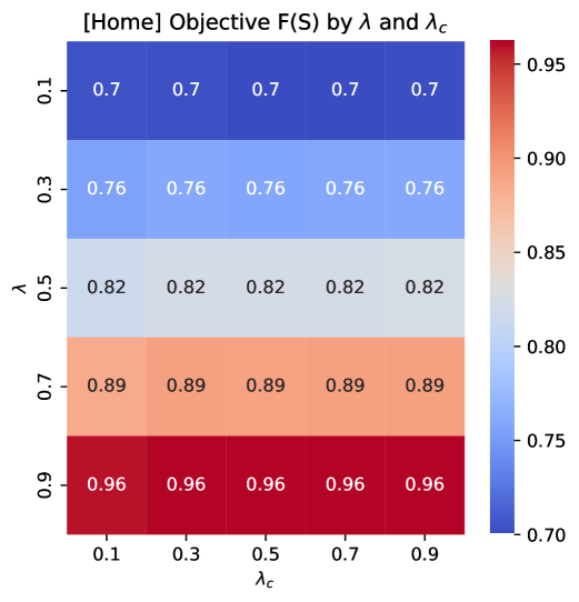
Figure 4: Diversity, quality, and the objective as the function of $\lambda_{c}$ and $\lambda$ for Home dataset with size of $|{\mathcal{U}}|=4737$.

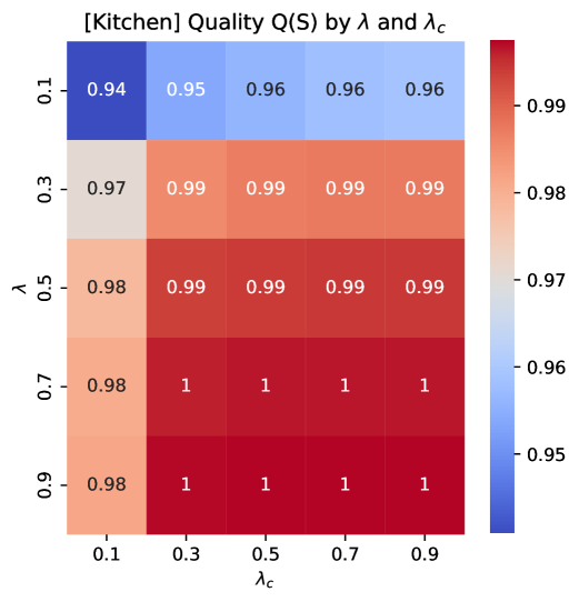
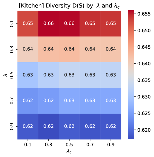
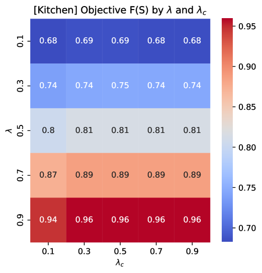
Figure 5: Diversity, quality, and the objective as the function of $\lambda_{c}$ and $\lambda$ for Kitchen dataset with size of $|{\mathcal{U}}|=3872$

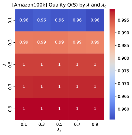
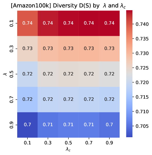
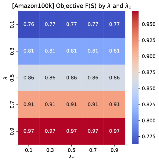
Figure 6: Diversity, quality, and the objective as the function of $\lambda_{c}$ and $\lambda$ for Amazon100k dataset with size of $|{\mathcal{U}}|=108,258$.

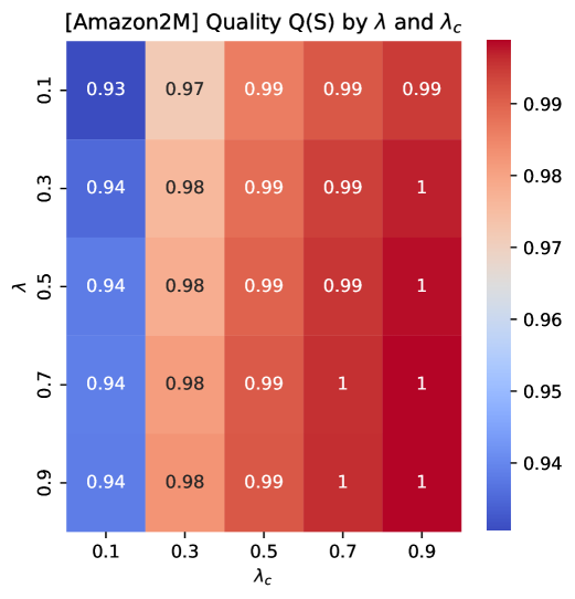
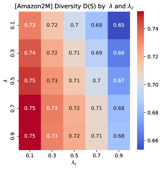
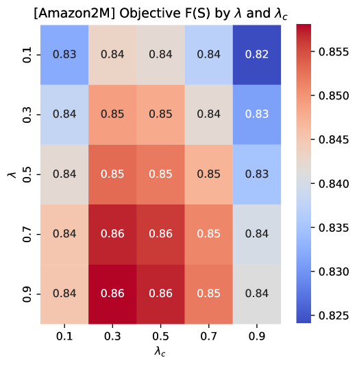
Figure 7: Diversity, quality, and the objective as the function of $\lambda_{c}$ and $\lambda$ for Amazon2M dataset with size of $|{\mathcal{U}}|=2M$.

C.4 Computational Time for each Component in dgds and muss

In Figure 8, we measure and report computational time spent in each component of Algorithm 2. This includes clustering (Line 1), greedy cluster selection (Line 3), greedy item selection in each selected cluster (Line 5), and the final selection ${\mathcal{S}}$ (Line 6). In this setting, we select $k=500$ items from Amazon100k and Amazon2M datasets using $m=100$ and $l=200$. We use different colors to indicate time spent in different steps. Clustering and cluster selection take negligible time compared to the time for selection within clusters (in blue) and the final selection (in red). Here, clustering can be done using scalalable libraries faiss [Douze et al., 2024] or MiniBatchKmeans [Sculley, 2010]. In particular, selection within each cluster takes the most time for Amazon2M dataset. This is because each cluster will have approximately $2M/200=10k$ items. There are $100$ clusters that are processed in parallel on $p=64$ CPUs. On the other hand, the selection from the items union has in the order of $500\times 100=50k$ points.

While the dgds does not spend time on clustering, it is slower than muss for two reasons: (i) there are more partitions ($l>m$) to be selecting from, and (ii) accordingly, after the union step $\cup_{i=1}^{l}{\mathcal{S}}_{i}$, the number of items is larger ($l\times k>m\times k$). We note that point (i) can be potentially addressed for dgds by using number of CPUs $p=l$. However, point (ii) remains a bottleneck for dgds irrespective of getting more CPUs.

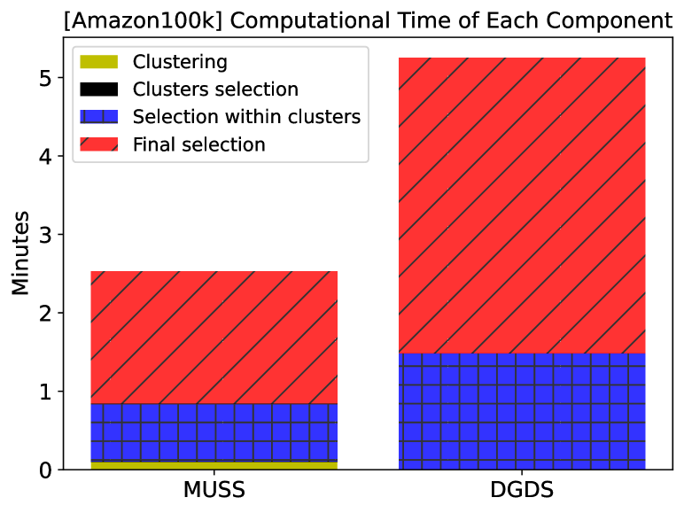
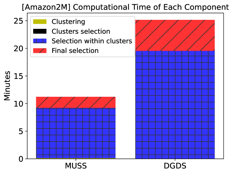
Figure 8: Computational time taken by each component of the Algorithm 2, compared against similar steps of dgds. Our method is more computationally efficient due to having a smaller number of partitions and fewer data points in the final selection step (Line 6 Algorithm 2).

C.5 Comparison of Clustering with and without the Quality Component

Our theoretical result in Theorem 6 shows that a good clustering structure can lead to better bound on the subset selection objective and thus better performance. This is, in particular, captured by the radius $r$ over the feature space and the quality radius $r_{q}$ over the quality space.

Therefore, we empirically analyze the performance by comparing clustering options with and without the quality score. We consider a regular clustering setting over the feature space ${\bm{x}}\in{\mathbb{R}}^{d}$ and clustering over a joint space of features and quality score $[{\bm{x}},q]\in{\mathbb{R}}^{d+1}$ as explained in Appendix B.

We present results in Table 7, where we used weighting parameter value of $w_{c}=1$ (see Eq. 55). For Home dataset, using the joint clustering space over features and quality can result in better performance for $4$ over $5$ cases w.r.t. the Precision. On the other hand, for Amazon100k dataset, the joint space does not improve the performance in terms of precision while it leads to comparable performance in terms of objective score of $0.97$. While including the quality dimension in clustering can lead to smaller radius $r_{q}$, the $r$ radius might increase. Thus performance gain is not guaranteed, and we observe mixed results.

Both options of clustering over ${\bm{x}}$ or $[{\bm{x}},q]$ result in similar running time because adding one more dimension to ${\mathbb{R}}^{d}$, when $d=1024$ has a negligible effect on execution time.

Table 7: Precision achieved by muss with clustering over feature space ${\bm{x}}\in{\mathbb{R}}^{d}$ and over the combined feature and quality space $[{\bm{x}},q]\in{\mathbb{R}}^{d+1}$

Home ($|{\mathcal{U}}|=4737$, $\lambda=0.9$)
$\lambda_{c}$	Clustering Space	Precision $\uparrow$	Objective $\uparrow$	Quality $\uparrow$	Diversity $\uparrow$	Time $\downarrow$
0.1	feature $[x]$	64.2	0.960	0.997	0.643	7.12
	feature and quality $[x,q]$	67.2	0.961	0.998	0.640	7.30
0.3	feature $[x]$	69.4	0.962	0.998	0.633	7.86
	feature and quality $[x,q]$	64.4	0.960	0.995	0.646	7.71
0.5	feature $[x]$	69.0	0.962	0.998	0.634	8.91
	feature and quality $[x,q]$	70.2	0.963	0.998	0.642	8.97
0.7	feature $[x]$	68.6	0.962	0.998	0.634	9.17
	feature and quality $[x,q]$	70.6	0.963	0.998	0.643	9.14
0.9	feature $[x]$	69.2	0.962	0.998	0.636	8.18
	feature and quality $[x,q]$	69.8	0.963	0.998	0.643	8.06

Amazon100K ($|{\mathcal{U}}|=108,258$, $\lambda=0.9$)
$\lambda_{c}$	Clustering Space	Precision $\uparrow$	Objective $\uparrow$	Quality $\uparrow$	Diversity $\uparrow$	Time $\downarrow$
0.1	feature $[x]$	41.0	0.97	0.999	0.703	128
	feature and quality $[x,q]$	38.8	0.97	0.999	0.703	127
0.3	feature $[x]$	42.4	0.97	0.999	0.705	145
	feature and quality $[x,q]$	39.6	0.97	0.999	0.707	148
0.5	feature $[x]$	44.0	0.97	0.999	0.706	158
	feature and quality $[x,q]$	38.4	0.97	0.999	0.710	160
0.7	feature $[x]$	44.4	0.97	0.999	0.706	166
	feature and quality $[x,q]$	39.2	0.97	0.999	0.710	165
0.9	feature $[x]$	43.8	0.97	0.999	0.705	159
	feature and quality $[x,q]$	40.8	0.97	0.999	0.710	159

C.6 Comparing Greedy Objectives

In our results, mmr denotes the sum-based greedy selection criterion as per Algorithm 1 (“sum-distance” criterion). We have also evaluated greedy selection using the original maximum similarity criterion [Carbonell and Goldstein, 1998].

$$\text{MMR}^{\prime}(s)=\lambda\cdot\text{Sim}(s,z)-(1-\lambda)\cdot\max_{t\in{\mathcal{S}}}\text{Sim}(s,t).$$ (59)

Here, $z$ is the query for which mmr is performed, and ${\mathcal{S}}$ is the subset selected so far. For our quality and distance functions this criterion becomes

$$\text{MMR}^{\prime}(s)=\lambda\cdot q(s)+(1-\lambda)\cdot\min_{t\in{\mathcal{S}}}d(s,t).$$ (60)

Overall the results were slightly worse compared to the “sum-distance” criterion, see Table 8.

Table 8: Precision achieved by muss using either “sum distance” or “min distance” as the greedy selection criterion.

Home ($|{\mathcal{U}}|=4737$, $\lambda=0.9$)
$\lambda_{c}$	Diversity Distance	Precision $\uparrow$	Objective $\uparrow$	Quality $\uparrow$	Diversity $\uparrow$	Time $\downarrow$
0.1	sum distance	63.6	0.889	0.996	0.643	7.12
	min distance	63.2	0.879	0.979	0.654	7.30
0.3	sum distance	66.6	0.892	0.997	0.646	7.86
	min distance	62.2	0.886	0.989	0.647	7.71
0.5	sum distance	66.6	0.892	0.997	0.646	8.91
	min distance	64.0	0.887	0.994	0.642	8.97
0.7	sum distance	66.6	0.892	0.997	0.647	9.17
	min distance	63.4	0.887	0.994	0.638	9.14
0.9	sum distance	66.8	0.892	0.997	0.648	8.18
	min distance	65.0	0.888	0.995	0.639	8.06

Amazon100K ($|{\mathcal{U}}|=108,258$, $\lambda=0.9$)
$\lambda_{c}$	Diversity Distance	Precision $\uparrow$	Objective $\uparrow$	Quality $\uparrow$	Diversity $\uparrow$	Time $\downarrow$
0.1	sum distance	41.0	0.970	0.999	0.703	128
	min distance	30.8	0.967	0.999	0.687	127
0.3	sum distance	42.4	0.970	0.999	0.705	145
	min distance	36.0	0.967	0.999	0.688	148
0.5	sum distance	44.0	0.970	0.999	0.706	166
	min distance	38.4	0.968	0.999	0.687	165
0.7	sum distance	44.4	0.970	0.999	0.706	158
	min distance	38.8	0.968	0.999	0.688	160
0.9	sum distance	43.8	0.970	0.999	0.705	159
	min distance	39.2	0.970	0.999	0.710	159

References

- Acharya et al. [2024] Abhinab Acharya, Dayou Yu, Qi Yu, and Xumin Liu. Balancing feature similarity and label variability for optimal size-aware one-shot subset selection. In Forty-first International Conference on Machine Learning, 2024.
- Baeza-Yates [2005] Ricardo Baeza-Yates. Applications of web query mining. In European Conference on Information Retrieval, pages 7–22. Springer, 2005.
- Barbosa et al. [2015] Rafael Barbosa, Alina Ene, Huy Nguyen, and Justin Ward. The power of randomization: Distributed submodular maximization on massive datasets. In International Conference on Machine Learning, pages 1236–1244. PMLR, 2015.
- Borodin et al. [2017] Allan Borodin, Aadhar Jain, Hyun Chul Lee, and Yuli Ye. Max-sum diversification, monotone submodular functions, and dynamic updates. ACM Transactions on Algorithms (TALG), 13(3):1–25, 2017.
- Carbonell and Goldstein [1998] Jaime Carbonell and Jade Goldstein. The use of mmr, diversity-based reranking for reordering documents and producing summaries. In Proceedings of the 21st annual international ACM SIGIR conference on Research and development in information retrieval, pages 335–336, 1998.
- Carraro and Bridge [2024] Diego Carraro and Derek Bridge. Enhancing recommendation diversity by re-ranking with large language models. ACM Transactions on Recommender Systems, 2024.
- Clarke et al. [2008] Charles LA Clarke, Maheedhar Kolla, Gordon V Cormack, Olga Vechtomova, Azin Ashkan, Stefan Büttcher, and Ian MacKinnon. Novelty and diversity in information retrieval evaluation. In Proceedings of the 31st annual international ACM SIGIR conference on Research and development in information retrieval, pages 659–666, 2008.
- Coppolillo et al. [2024] Erica Coppolillo, Giuseppe Manco, and Aristides Gionis. Relevance meets diversity: A user-centric framework for knowledge exploration through recommendations. In Proceedings of the 30th ACM SIGKDD Conference on Knowledge Discovery and Data Mining, pages 490–501, 2024.
- Derezinski et al. [2019] Michal Derezinski, Daniele Calandriello, and Michal Valko. Exact sampling of determinantal point processes with sublinear time preprocessing. Advances in neural information processing systems, 32, 2019.
- Douze et al. [2024] Matthijs Douze, Alexandr Guzhva, Chengqi Deng, Jeff Johnson, Gergely Szilvasy, Pierre-Emmanuel Mazaré, Maria Lomeli, Lucas Hosseini, and Hervé Jégou. The faiss library. arXiv preprint arXiv:2401.08281, 2024.
- El-Kishky et al. [2023] Ahmed El-Kishky, Thomas Markovich, Kenny Leung, Frank Portman, Aria Haghighi, and Ying Xiao. k nn-embed: Locally smoothed embedding mixtures for multi-interest candidate retrieval. In Pacific-Asia Conference on Knowledge Discovery and Data Mining, pages 374–386. Springer, 2023.
- Elfeki et al. [2019] Mohamed Elfeki, Camille Couprie, Morgane Riviere, and Mohamed Elhoseiny. Gdpp: Learning diverse generations using determinantal point processes. In International conference on machine learning, pages 1774–1783. PMLR, 2019.
- Erkan and Radev [2004] Günes Erkan and Dragomir R Radev. Lexrank: Graph-based lexical centrality as salience in text summarization. Journal of artificial intelligence research, 22:457–479, 2004.
- Fabbri et al. [2021] Alexander R Fabbri, Wojciech Kryściński, Bryan McCann, Caiming Xiong, Richard Socher, and Dragomir Radev. Summeval: Re-evaluating summarization evaluation. Transactions of the Association for Computational Linguistics, 9:391–409, 2021.
- Fontaine and Nikolaidis [2021] Matthew Fontaine and Stefanos Nikolaidis. Differentiable quality diversity. Advances in Neural Information Processing Systems, 34:10040–10052, 2021.
- Gao and Zhang [2024] Hang Gao and Yongfeng Zhang. Vrsd: Rethinking similarity and diversity for retrieval in large language models. arXiv preprint arXiv:2407.04573, 2024.
- Ge et al. [2024] Yuan Ge, Yilun Liu, Chi Hu, Weibin Meng, Shimin Tao, Xiaofeng Zhao, Hongxia Ma, Li Zhang, Boxing Chen, Hao Yang, et al. Clustering and ranking: Diversity-preserved instruction selection through expert-aligned quality estimation. arXiv preprint arXiv:2402.18191, 2024.
- Ghadiri and Schmidt [2019] Mehrdad Ghadiri and Mark Schmidt. Distributed maximization of submodular plus diversity functions for multi-label feature selection on huge datasets. In The 22nd International Conference on Artificial Intelligence and Statistics, pages 2077–2086. PMLR, 2019.
- Gong et al. [2019] Zhiqiang Gong, Ping Zhong, and Weidong Hu. Diversity in machine learning. Ieee Access, 7:64323–64350, 2019.
- Guinet et al. [2024] Gauthier Guinet, Behrooz Omidvar-Tehrani, Anoop Deoras, and Laurent Callot. Automated evaluation of retrieval-augmented language models with task-specific exam generation. arXiv preprint arXiv:2405.13622, 2024.
- Guo and Sanner [2010] Shengbo Guo and Scott Sanner. Probabilistic latent maximal marginal relevance. In Proceedings of the 33rd international ACM SIGIR conference on Research and development in information retrieval, pages 833–834, 2010.
- He et al. [2012] Jingrui He, Hanghang Tong, Qiaozhu Mei, and Boleslaw Szymanski. Gender: A generic diversified ranking algorithm. Advances in neural information processing systems, 25, 2012.
- Hirata et al. [2022] Kohei Hirata, Daichi Amagata, Sumio Fujita, and Takahiro Hara. Solving diversity-aware maximum inner product search efficiently and effectively. In Proceedings of the 16th ACM Conference on Recommender Systems, pages 198–207, 2022.
- Kulesza and Taskar [2011] Alex Kulesza and Ben Taskar. k-dpps: Fixed-size determinantal point processes. In Proceedings of the 28th International Conference on Machine Learning (ICML-11), pages 1193–1200, 2011.
- Kulesza et al. [2012] Alex Kulesza, Ben Taskar, et al. Determinantal point processes for machine learning. Foundations and Trends® in Machine Learning, 5(2–3):123–286, 2012.
- Levine et al. [2020] Sergey Levine, Aviral Kumar, George Tucker, and Justin Fu. Offline reinforcement learning: Tutorial, review, and perspectives on open problems. arXiv preprint arXiv:2005.01643, 2020.
- Li et al. [2016] Chengtao Li, Stefanie Jegelka, and Suvrit Sra. Efficient sampling for k-determinantal point processes. In Artificial Intelligence and Statistics, pages 1328–1337. PMLR, 2016.
- Lloyd [1982] Stuart Lloyd. Least squares quantization in pcm. IEEE transactions on information theory, 28(2):129–137, 1982.
- Luan et al. [2018] WenJing Luan, GuanJun Liu, ChangJun Jiang, and MengChu Zhou. Mptr: A maximal-marginal-relevance-based personalized trip recommendation method. IEEE Transactions on Intelligent Transportation Systems, 19(11):3461–3474, 2018.
- Maharana et al. [2023] Adyasha Maharana, Prateek Yadav, and Mohit Bansal. D2 pruning: Message passing for balancing diversity and difficulty in data pruning. arXiv preprint arXiv:2310.07931, 2023.
- Mihaylov et al. [2018] Todor Mihaylov, Peter Clark, Tushar Khot, and Ashish Sabharwal. Can a suit of armor conduct electricity? a new dataset for open book question answering. In EMNLP, 2018.
- Mirzasoleiman et al. [2016] Baharan Mirzasoleiman, Amin Karbasi, Rik Sarkar, and Andreas Krause. Distributed submodular maximization. The Journal of Machine Learning Research, 17(1):8330–8373, 2016.
- Nemhauser et al. [1978] George L Nemhauser, Laurence A Wolsey, and Marshall L Fisher. An analysis of approximations for maximizing submodular set functions—i. Mathematical programming, 14:265–294, 1978.
- Nguyen et al. [2021] Vu Nguyen, Tam Le, Makoto Yamada, and Michael A Osborne. Optimal transport kernels for sequential and parallel neural architecture search. In International Conference on Machine Learning, pages 8084–8095. PMLR, 2021.
- Panteli and Boutsinas [2023] Antiopi Panteli and Basilis Boutsinas. Improvement of similarity–diversity trade-off in recommender systems based on a facility location model. Neural Computing and Applications, 35(1):177–189, 2023.
- Parker-Holder et al. [2020] Jack Parker-Holder, Aldo Pacchiano, Krzysztof M Choromanski, and Stephen J Roberts. Effective diversity in population based reinforcement learning. Advances in Neural Information Processing Systems, 33:18050–18062, 2020.
- Pickett et al. [2024] Marc Pickett, Jeremy Hartman, Ayan Kumar Bhowmick, Raquib-ul Alam, and Aditya Vempaty. Better RAG using relevant information gain. arXiv preprint arXiv:2407.12101, 2024.
- Qin et al. [2012] L Qin, JX Yu, and L Chang. Diversifying top- results. Proceedings of the VLDB Endowment, 2012.
- Rajput et al. [2023] Shashank Rajput, Nikhil Mehta, Anima Singh, Raghunandan Hulikal Keshavan, Trung Vu, Lukasz Heldt, Lichan Hong, Yi Tay, Vinh Tran, Jonah Samost, et al. Recommender systems with generative retrieval. Advances in Neural Information Processing Systems, 36:10299–10315, 2023.
- Schneider et al. [2022] Lennart Schneider, Florian Pfisterer, Paul Kent, Juergen Branke, Bernd Bischl, and Janek Thomas. Tackling neural architecture search with quality diversity optimization. In International Conference on Automated Machine Learning, pages 9–1. PMLR, 2022.
- Sculley [2010] David Sculley. Web-scale k-means clustering. In Proceedings of the 19th international conference on World wide web, pages 1177–1178, 2010.
- Van der Maaten and Hinton [2008] Laurens Van der Maaten and Geoffrey Hinton. Visualizing data using t-sne. Journal of machine learning research, 9(11), 2008.
- Wan and Yang [2008] Xiaojun Wan and Jianwu Yang. Multi-document summarization using cluster-based link analysis. In Proceedings of the 31st annual international ACM SIGIR conference on Research and development in information retrieval, pages 299–306, 2008.
- Wang et al. [2021] Yutong Wang, Ke Xue, and Chao Qian. Evolutionary diversity optimization with clustering-based selection for reinforcement learning. In International Conference on Learning Representations, 2021.
- Wilhelm et al. [2018] Mark Wilhelm, Ajith Ramanathan, Alexander Bonomo, Sagar Jain, Ed H Chi, and Jennifer Gillenwater. Practical diversified recommendations on youtube with determinantal point processes. In Proceedings of the 27th ACM International Conference on Information and Knowledge Management, pages 2165–2173, 2018.
- Wu et al. [2023a] Chun-Ho Wu, Yue Wang, and Jie Ma. Maximal marginal relevance-based recommendation for product customisation. Enterprise Information Systems, 17(5):1992018, 2023a.
- Wu et al. [2023b] Shuang Wu, Jian Yao, Haobo Fu, Ye Tian, Chao Qian, Yaodong Yang, Qiang Fu, and Yang Wei. Quality-similar diversity via population based reinforcement learning. In The Eleventh International Conference on Learning Representations, 2023b.
- Xia et al. [2015] Long Xia, Jun Xu, Yanyan Lan, Jiafeng Guo, and Xueqi Cheng. Learning maximal marginal relevance model via directly optimizing diversity evaluation measures. In Proceedings of the 38th international ACM SIGIR conference on research and development in information retrieval, pages 113–122, 2015.
- Yuan and Kitani [2020] Ye Yuan and Kris M Kitani. Diverse trajectory forecasting with determinantal point processes. In International Conference on Learning Representations, 2020.