Convergence Analysis of EXTRA in Non-convex Distributed Optimization

Abstract

Optimization problems involving the minimization of a finite sum of smooth, possibly non-convex functions arise in numerous applications. To achieve a consensus solution over a network, distributed optimization algorithms, such as EXTRA (decentralized exact first-order algorithm), have been proposed to address these challenges. In this paper, we analyze the convergence properties of EXTRA in the context of smooth, non-convex optimization. By interpreting its updates as a nonlinear dynamical system, we show novel insights into its convergence properties. Specifically, i) EXTRA converges to a consensual first-order stationary point of the global objective with a sublinear rate; and ii) EXTRA avoids convergence to consensual strict saddle points, offering second-order guarantees that ensure robustness. These findings provide a deeper understanding of EXTRA in a non-convex context.

I Introduction

Optimization problems that involve a finite sum of functions formed as

$$\min_{\mathbf{x}\in\mathbb{R}^{n}}f(\mathbf{x})\triangleq\sum_{i=1}^{m}f_{i}(\mathbf{x}),$$ (1)

are central to a wide range of applications, including distributed machine learning [1, 2, 3], sensor networks[4, 5, 6], and large-scale control [7, 8, 9]. In such problems, the function $f_{i}\mathrel{\mathop{\ordinarycolon}}\mathbb{R}^{n}\rightarrow\mathbb{R}$ is often assumed to be smooth and possibly non-convex. A key challenge arises when $f_{i}$ represents data or tasks that are distributed across $m$ agents, such that each agent $i$ has access only to its local function $f_{i}$ and its gradient information. The agents must collaboratively minimize the global objective $f(x)$ while communicating over an undirected and interconnected network graph $\mathcal{G}(\mathcal{V},\mathcal{E})$. This graph consists of two key components: the set of agents $\mathcal{V}\mathrel{\mathop{\ordinarycolon}}=\{1,\ldots,m\}$, where each agent $i\in\mathcal{V}$ processes its local data, and the set of edges $\mathcal{E}\subseteq\mathcal{V}\times\mathcal{V}$, indicating that agents $i$ and $j$ can exchange information if $(i,j)\in\mathcal{E}$.

To address such optimization problems, distributed algorithms have been developed to enable agents to iteratively reach a consensus on the optimal solution. Among these algorithms, consensus-based gradient descent methods have gained significant attention due to their scalability and adaptability to network settings. Notable methods include Distributed Gradient Descent (DGD) [10, 11], and its variants [12, 13, 14, 15]. However, these methods often face limitations in terms of achieving exact consensus. A key breakthrough in distributed optimization was the introduction of the Exact First-Order Algorithm (EXTRA) in [16] and DIGing [17], which both improve on traditional consensus-based methods by achieving exact consensus. As EXTRA proposed in [16], the update for each agent $i\in\mathcal{V}$ in iteration $k\in\mathbb{N}$ is given by

$$\begin{gathered}\hat{\mathbf{x}}^{1}_{i}=\sum_{j=1}^{m}\mathbf{W}_{ij}\hat{\mathbf{x}}^{0}_{j}-\alpha\nabla f_{i}(\hat{\mathbf{x}}^{0}_{i}),\\ \hat{\mathbf{x}}^{k+2}_{i}=\hat{\mathbf{x}}^{k+1}_{i}+\sum_{j=1}^{m}\mathbf{W}_{ij}\hat{\mathbf{x}}^{k+1}_{j}-\sum_{j=1}^{m}\mathbf{V}_{ij}\hat{\mathbf{x}}^{k}_{j}\\ -\alpha[\nabla f_{i}(\hat{\mathbf{x}}^{k+1}_{i})-\nabla f_{i}(\hat{\mathbf{x}}^{k}_{i})],\end{gathered}$$ (5)

where $\hat{\mathbf{x}}_{i}\in\mathbb{R}^{n}$ is the local copy of the decision vector $\mathbf{x}$ at agent $i\in\mathcal{V}$, and $\hat{\mathbf{x}}=[\hat{\mathbf{x}}_{1}^{\top},\cdots,\hat{\mathbf{x}}_{m}^{\top}]^{\top}\in(\mathbb{R}^{n})^{m}$. $\alpha>0$ is the constant step-size, $\nabla f_{i}$ is the gradient of $f_{i}$, and $\mathbf{W}_{ij}$ (resp., $\mathbf{V}_{ij}$) is the scalar entry in the $i$-th row and $j$-th column of a given mixing matrix $\mathbf{W}\in\mathbb{R}^{m\times m}$ (resp., $\mathbf{V}\in\mathbb{R}^{m\times m}$). Compared to gradient tracking methods in [17], EXTRA is more free to choose two mixing matrices $\mathbf{W}$ and $\mathbf{V}$.

Despite its effectiveness, the theoretical analysis of the EXTRA algorithm has largely focused on settings where the objective function $f(x)$ is smooth and either convex or strongly convex. The original work on EXTRA [16] established linear convergence rates for strongly convex objectives and sublinear rates for general convex functions, providing a solid foundation for distributed optimization under these assumptions. Subsequently, the primal-dual-based method [18], which extends EXTRA, achieved similar convergence results in convex settings. Additionally, convergence results for EXTRA on directed graphs were established in [19], while extensions such as PG-EXTRA [20] have addressed non-smooth convex problems. However, in non-convex settings, theoretical results remain more limited. Recent studies, such as [21, 22], have started to explore the performance of primal-dual-based methods and gradient tracking methods in non-convex settings, focusing on the second-order guarantees.

This paper provides a novel perspective on the EXTRA algorithm by analyzing its update as a nonlinear dynamical system. Building on these insights, we establish both first-order and second-order convergence guarantees for EXTRA in the context of smooth and non-convex optimization:

1. In Theorem III.1, we model EXTRA as a nonlinear dynamic system. By assuming that the mixing matrices satisfy a linear combination property, we establish that EXTRA converges to a consensual first-order stationary point of the global objective. This result extends previous analyses by addressing the challenges posed by non-convexity.

2. In Theorem III.2, we establish that EXTRA avoids convergence to consensual strict saddle points of the global objective and eventually converge to a consensual second-order stationary point. This second-order guarantee underscores the algorithm’s robustness.

The above results can be found in Section III. Section II provides the assumptions and supporting results. Section IV provides complete proofs for the theoretical results. Section V provides a numerical example.

I-A Notation

Let $\mathbf{I}_{n}$ denote the $n\times n$ identity matrix, $\bm{1}_{n}$ denote the $n$-vector with all entries equal to $1$, and $\mathbf{A}_{ij}$ denote the entry in row $i$ and column $j$ of the matrix $\mathbf{A}$. For a square symmetric matrix $\mathbf{B}$, we use $\lambda_{\mathrm{min}}(\mathbf{B})$, $\lambda_{\mathrm{max}}(\mathbf{B})$, and $\|\mathbf{B}\|$ to denote its minimum eigenvalue, maximum eigenvalue, and spectral norm, respectively. For a square matrix $\mathbf{C}$, we use $\lambda_{i}(\mathbf{C})\geq 0$ to denote its $i$-th largest magnitude eigenvalue. The distance from the point $\mathbf{x}\in\mathbb{R}^{n}$ to a given set $\mathcal{Y}\subseteq\mathbb{R}^{n}$ is denoted by $\textup{dist}(\mathbf{x},\mathcal{Y})\coloneqq\inf_{\mathbf{y}\in\mathcal{Y}}\|\mathbf{x}-\mathbf{y}\|$. The Kronecker product is denoted by $\otimes$. Unless explicitly stated otherwise, all iterated parameters in this paper are positive integers.

II Assumptions and Supporting Results

II-A Definitions and Assumptions

Definition II.1

For differentiable function $h\mathrel{\mathop{\ordinarycolon}}\mathbb{R}^{n}\rightarrow\mathbb{R}$, a point $\mathbf{x}$ is said to be first-order stationary if $\|\nabla h(\mathbf{x})\|=0$, where $\nabla h$ denotes the gradient of $h$.

Assumption II.1 (Lipschitz continuity)

Each $f_{i}$ in (1) is $L_{f_{i}}^{g}$-gradient Lipschitz, i.e., for all $\mathbf{x},\mathbf{y}\in\mathbb{R}^{n}$ and each $i\in\mathcal{V}$, $\|\nabla f_{i}(\mathbf{x})-\nabla f_{i}(\mathbf{y})\|\leq L_{f_{i}}^{g}\|\mathbf{x}-\mathbf{y}\|$.

Assumption II.2 (Coercivity and properness)

Each $f_{i}$ in (1) is coercive (i.e., its sublevel set is compact) and proper (i.e., not everywhere infinite).

Assumption II.3 (Connect network)

The undirected network graph $\mathcal{G}(\mathcal{V},\mathcal{E})$ is connected.

Assumption II.4 (Mixing matrix)

The mixing matrices of network $\mathcal{G}$, $\mathbf{W}\in\mathbb{R}^{m\times m}$ and $\mathbf{V}\in\mathbb{R}^{m\times m}$ satisfy:

• If $(i,j)\notin\mathcal{E}$ and $i\neq j$, then $\mathbf{W}_{ij}=0$.

• $\mathbf{W}=\mathbf{W}^{\top}$.

• $-\mathbf{I}_{m}\prec\mathbf{W}\preceq\mathbf{I}_{m}$ and $\textup{null}\{\mathbf{I}_{m}-\mathbf{W}\}=\textup{span}\{\bm{1}\}$.

• $\mathbf{V}=\theta\mathbf{I}_{m}+(1-\theta)\mathbf{W}$, with $\theta\in(0,\frac{1}{2}]$.

Remark 1

The fourth condition in Assumption II.4 can be extended to linear combination of $\mathbf{I}_{m}$ and high-order terms of $\mathbf{W}$, $i.e.$, $\mathbf{V}=\sum_{i=0}^{n}\theta_{i}\mathbf{W}^{i}$, where $\sum_{i=1}^{n}\theta_{i}=1$, and our results still hold. For example, DIGing (or Gradient Tracking) algorithm in [17] uses $\mathbf{V}=\frac{1}{4}\mathbf{W}^{2}+\frac{1}{2}\mathbf{W}+\frac{1}{4}\mathbf{I}$. However, the high-order terms of $\mathbf{W}$ require multiple communication steps at each iteration of the distributed algorithm.

II-B Algorithm Review and Supporting Results

To study distributed algorithms, we first need to reformulate the objective function in (1) as

$$\begin{gathered}F\mathrel{\mathop{\ordinarycolon}}~(\mathbb{R}^{n})^{m}\rightarrow\mathbb{R},~F(\hat{\mathbf{x}})\triangleq\sum_{i=1}^{m}f_{i}(\hat{\mathbf{x}}_{i}),\end{gathered}$$ (7)

where $\hat{\mathbf{x}}=[\hat{\mathbf{x}}_{1}^{\top},\cdots,\hat{\mathbf{x}}_{m}^{\top}]^{\top}\in(\mathbb{R}^{n})^{m}$ with each $\hat{\mathbf{x}}_{i}\in\mathbb{R}^{n}$. Note that, $\nabla F(\hat{\mathbf{x}})=[\nabla f_{1}(\hat{\mathbf{x}}_{1})^{\top},\cdots,\nabla f_{m}(\hat{\mathbf{x}}_{m})^{\top}]^{\top}$ and $\nabla^{2}F(\hat{\mathbf{x}})=\bigoplus_{i=1}^{m}\nabla^{2}f_{i}(\hat{\mathbf{x}}_{i})$. In particular, the Hessian of $F$ is block diagonal. Then, the following result can be derived directly.

Proposition II.1

Let Assumption II.1 hold. $F$ defined in (7) has $L_{F}^{g}$-Lipschitz continuous gradient with $L_{F}^{g}=\max_{i}\{L_{f_{i}}^{g}\}$.

Next, we define the consensual first-order stationary point for $F$ in (7).

Definition II.2

For function $F$ in (7), a point $\hat{\mathbf{x}}\in(\mathbb{R}^{n})^{m}$ is said to be a consensual first-order stationary point if

1. $\hat{\mathbf{x}}=\frac{1}{m}(\bm{1}_{m}\bm{1}_{m}^{\top}\otimes\mathbf{I}_{n})\hat{\mathbf{x}}$;

2. $(\bm{1}_{m}\otimes\mathbf{I}_{n})^{\top}\nabla F(\hat{\mathbf{x}})=\sum_{i=1}^{m}\nabla f_{i}(\hat{\mathbf{x}}_{i})=0$.

If condition 1) holds, then the point $\hat{\mathbf{x}}$ is in consensus, $i.e.$, $\hat{\mathbf{x}}_{i}=\hat{\mathbf{x}}_{j}$ for all $i$, $j\in\mathcal{V}$. Furthermore, if condition 2) also holds, then for any $i\in\mathcal{V}$, $\hat{\mathbf{x}}_{i}$ is a first-order stationary point of $f$ (see Proposition 2.1 in [16]).

Recall the standard fixed step-size EXTRA algorithm as in (5), and it can be written in a matrix/vector form as $\hat{\mathbf{x}}^{1}=\hat{\mathbf{W}}\hat{\mathbf{x}}^{0}-\alpha\nabla F(\hat{\mathbf{x}}^{0})$, $\hat{\mathbf{x}}^{k+2}=\hat{\mathbf{x}}^{k+1}+\hat{\mathbf{W}}\hat{\mathbf{x}}^{k+1}-\hat{\mathbf{V}}\hat{\mathbf{x}}^{k}-\alpha[\nabla F(\hat{\mathbf{x}}^{k+1})-\nabla F(\hat{\mathbf{x}}^{k})]$, where $\hat{\mathbf{W}}=\mathbf{W}\otimes\mathbf{I}_{n}$ and $\hat{\mathbf{V}}=\mathbf{V}\otimes\mathbf{I}_{n}$. Let $\hat{\mathbf{z}}^{k}=\hat{\mathbf{x}}^{k+1}-\hat{\mathbf{W}}\hat{\mathbf{x}}^{k}$. Then, with $\hat{\mathbf{z}}^{0}=-\alpha\nabla F(\hat{\mathbf{x}}^{0})$, EXTRA can be formulated as a dynamical system:

$$\begin{gathered}\hat{\mathbf{x}}^{k+1}=\hat{\mathbf{W}}\hat{\mathbf{x}}^{k}+\hat{\mathbf{z}}^{k},\\ \hat{\mathbf{z}}^{k+1}=(\hat{\mathbf{W}}-\hat{\mathbf{V}})\hat{\mathbf{x}}^{k}+\hat{\mathbf{z}}^{k}-\alpha[\nabla F(\hat{\mathbf{x}}^{k+1})-\nabla F(\hat{\mathbf{x}}^{k})].\end{gathered}$$ (10)

III Main Results

We study the first-order and second-order convergence properties of EXTRA using the dynamical model in (10).

III-A Properties of Mixing Matrices

Based on this non-linear system in (10), we first derived key properties of the mixing matrices, which are used in the proof of Theorem III.1.

Lemma III.1

Let Assumptions II.4 hold. Let

$$\mathbf{P}=\begin{bmatrix}\mathbf{W}-\frac{1}{m}\bm{1}_{m}\bm{1}_{m}^{\top}&\mathbf{I}_{m}\\ \mathbf{W}-\mathbf{V}&\mathbf{I}_{m}-\frac{1}{m}\bm{1}_{m}\bm{1}_{m}^{\top}\end{bmatrix},$$ (11)

then it holds that $\lambda_{1}(\mathbf{P})<1$, where $\lambda_{1}(\mathbf{P})$ denotes the largest magnitude eigenvalue of $\mathbf{P}$.

III-B Convergence guarantees of EXTRA

The following main results establish the first-order and second-order guarantees of EXTRA. First, Theorem III.1 shows that EXTRA converges to a consensual first-order stationary point of $F$.

Theorem III.1

Let Assumptions II.1, II.2, II.3, II.4 holds. For any fixed step-size

$$0<\alpha<\frac{1-(\lambda_{1}(\mathbf{P}))^{2}}{6(L_{F}^{g})^{4}+6(L_{F}^{g})^{3}+48L_{F}^{g}+1},$$ (12)

where $\mathbf{P}$ is defined in (11), it holds that the sequence $\{\hat{\mathbf{x}}^{k}\}$ generated by (5) satisfies that

$$\frac{1}{k}\sum_{\kappa=0}^{k-1}\mathinner{\!\left\lVert(\mathbf{I}_{mn}-\frac{1}{m}(\bm{1}_{m}\bm{1}_{m}^{\top})\otimes\mathbf{I}_{n})\hat{\mathbf{x}}^{\kappa}\right\rVert}^{2}=\mathcal{O}(\frac{1}{k}),$$

$$\frac{1}{k}\sum_{\kappa=0}^{k-1}\mathinner{\!\left\lVert\frac{1}{m}(\bm{1}_{m}\bm{1}_{m}^{\top})\otimes\mathbf{I}_{n}\cdot\nabla F(\hat{\mathbf{x}}^{\kappa})\right\rVert}^{2}=\mathcal{O}(\frac{1}{k}).$$

Remark 2

The convergence rate $\mathcal{O}(\frac{1}{k})$ in Theorem III.1 implies $\liminf_{k\rightarrow\infty}\mathinner{\!\left\lVert(\mathbf{I}_{mn}-\frac{1}{m}(\bm{1}_{m}\bm{1}_{m}^{\top})\otimes\mathbf{I}_{n})\hat{\mathbf{x}}^{k}\right\rVert}\leq C\frac{1}{k}$, and $\liminf_{k\rightarrow\infty}\mathinner{\!\left\lVert\frac{1}{m}(\bm{1}_{m}\bm{1}_{m}^{\top})\otimes\mathbf{I}_{n}\cdot\nabla F(\hat{\mathbf{x}}^{k})\right\rVert}\leq C\frac{1}{k}$ for some constant $C>0$, which corresponds to condition 1) and 2) in Definition II.2, respectively.

We next define the consensual second-order stationary point (consensual local minimizer) for $F$ in (7). The main result presented next establishes the second-order properties of EXTRA.

Definition III.1

For function $F$ in (7), a point $\hat{\mathbf{x}}\in(\mathbb{R}^{n})^{m}$ is said to be a consensual second-order stationary point if it satisfies the following:

1. $\hat{\mathbf{x}}=\frac{1}{m}(\bm{1}_{m}\bm{1}_{m}^{\top}\otimes\mathbf{I}_{n})\hat{\mathbf{x}}$;

2. $(\bm{1}_{m}\otimes\mathbf{I}_{n})^{\top}\nabla F(\hat{\mathbf{x}})=\sum_{i=1}^{m}\nabla f_{i}(\hat{\mathbf{x}}_{i})=0$;

3. $(\bm{1}_{m}\otimes\mathbf{I}_{n})^{\top}\nabla^{2}F(\hat{\mathbf{x}})(\bm{1}_{m}\otimes\mathbf{I}_{n})=\sum_{i=1}^{m}\nabla^{2}f_{i}(\hat{\mathbf{x}}_{i})\succeq 0$.

Let $\mathcal{X}_{c2}$ denote the set of consensual second-order stationary points of $F$.

Second, Theorem III.2 demonstrates that EXTRA converges almost surely to a consensual second-order stationary point of $F$.

Theorem III.2

Let Assumptions II.1-II.4 holds. For any fixed

$$0<\alpha<\min\{\frac{1-(\lambda_{1}(\mathbf{P}))^{2}}{6(L_{F}^{g})^{4}+6(L_{F}^{g})^{3}+48L_{F}^{g}+1},~\frac{\lambda_{\min}(\mathbf{V})}{L_{F}^{g}}\},$$

it holds that the sequence $\{\hat{\mathbf{x}}^{k}\}$ generated by (5) satisfies that

$$\mathbb{P}\left[\lim_{k\rightarrow\infty}\text{dist}(\hat{\mathbf{x}}^{k},\mathcal{X}_{c2})=0\right]=1.$$

IV Proofs

IV-A Proof for Lemma III.1

Proof:

Let $\mathbf{P}=\mathbf{M}-\mathbf{N}$, where

$$\begin{gathered}\mathbf{M}=\begin{bmatrix}\mathbf{W}&\mathbf{I}_{m}\\ \mathbf{W}-\mathbf{V}&\mathbf{I}_{m}\end{bmatrix},~\mathbf{N}=\begin{bmatrix}\frac{1}{m}\bm{1}_{m}\bm{1}_{m}^{\top}&\bm{0}\\ \bm{0}&\frac{1}{m}\bm{1}_{m}\bm{1}_{m}^{\top}\end{bmatrix}.\end{gathered}$$

To analyze the eigenvalue of $\mathbf{P}=\mathbf{M}-\mathbf{N}$, we first analyze the eigenvalue of $\mathbf{M}$ by $\det{(\mathbf{M}-\lambda\cdot\mathbf{I}_{2m})}=0$ with

$$\det{(\mathbf{M}-\lambda\mathbf{I}_{2m})}=\det{\left(\begin{bmatrix}\mathbf{W}-\lambda\mathbf{I}_{m}&\mathbf{I}_{m}\\ \mathbf{W}-\mathbf{V}&\mathbf{I}_{m}-\lambda\mathbf{I}_{m}\end{bmatrix}\right)}.$$ (13)

By Schur complement and Assumption II.4, (13) gives

$$\det{(\mathbf{M})} =(1-\lambda)^{m}\cdot\det{(\mathbf{W}-\lambda\mathbf{I}_{m}-\frac{1}{1-\lambda}\theta(\mathbf{W}-\mathbf{I}_{m}))}$$

$$=(1-\lambda)^{m}\cdot\prod_{i=1}^{m}\omega^{i}(1-\frac{\theta}{1-\lambda})+(\frac{\theta}{1-\lambda}-\lambda),$$

where $\omega^{i}\in(-1,1]$ is the $i$-th eigenvalue of $\mathbf{W}$ and $\theta\in(0,\frac{1}{2}]$.

Case 1: For $i\in\mathcal{V}$ such that $\omega^{i}=1$, $1$ is the only one solution to $\det{(\mathbf{M})}=0$.

Case 2: For $i\in\mathcal{V}$ such that $\omega^{i}\neq 1$ and $(1-\omega^{i})^{2}-4(1-\omega^{i})\theta\geq 0$ holds, which means all solutions satisfy

$$\prod_{i=1}^{m}\lambda^{2}-(1+\omega^{i})\lambda+\omega^{i}-\theta\omega^{i}+\theta=0,$$ (14)

and are all real. Since $1-\omega^{i}>0$ for all $i\in\mathcal{V}$ and $\theta\in(0,\frac{1}{2}]$, then $\mathinner{\!\left\lvert\lambda\right\rvert}\leq\frac{1+\omega^{i}+\sqrt{(1-\omega^{i})^{2}-4(1-\omega^{i})\theta}}{2}<\frac{1+\omega^{i}+\sqrt{(1-\omega^{i})^{2}}}{2}\leq 1$.

Case 3: For $i\in\mathcal{V}$ such that $\omega^{i}\neq 1$ and $(1-\omega^{i})^{2}-4(1-\omega^{i})\theta<0$ holds, which means all solutions satisfy (14) and are all complex. Then, $\mathinner{\!\left\lvert\lambda\right\rvert}\leq\omega^{i}-\theta\omega^{i}+\theta=\omega^{i}+\theta(1-\omega^{i})\leq\frac{1}{2}+\frac{1}{2}\omega^{i}<1$.

Combining three cases above, we conclude that, except for the eigenvalue $1$, the magnitude of eigenvalue of $\mathbf{M}$ is strictly less than $1$. Next, we focus on the eigenvector corresponding to the eigenvalue $1$ of $\mathbf{M}$. Suppose $\lambda=1$, which means $1$ is the eigenvalue of $\mathbf{M}$ and it holds that there exists nonzero vector $\mathbf{v}=[\mathbf{v}_{1}^{\top},\mathbf{v}_{2}^{\top}]^{\top}\in\mathbb{R}^{2m}$ such that $\mathbf{M}\mathbf{v}=\mathbf{v}$. Therefore, $(\mathbf{W}-\mathbf{V})\mathbf{v}_{1}=\bm{0}$ holds which implies $(\mathbf{I}_{m}-\mathbf{W})\mathbf{v}_{1}=\bm{0}$ by Assumption II.4. Since that $\mathbf{W}\mathbf{v}_{1}+\mathbf{v}_{2}=\mathbf{v}_{1}$, then $\mathbf{v}=[\frac{1}{\sqrt{m}}\bm{1}^{\top},\bm{0}]$ is the eigenvector corresponding to the eigenvalue $1$ of $\mathbf{M}$. Note that $\mathbf{v}=[\frac{1}{\sqrt{m}}\bm{1}^{\top},\bm{0}]^{\top}$ is also an eigenvector of $\mathbf{N}$ with eigenvalue $1$ and all other eigenvectors of $\mathbf{N}$ correspond to eigenvalue $0$. Thus, subtracting $\mathbf{N}$ from $\mathbf{M}$ eliminates the eigenvalue corresponding to the eigenvector $\mathbf{v}=[\frac{1}{\sqrt{m}}\bm{1}^{\top},\bm{0}]^{\top}$, thereby reducing the eigenvalue from 1 to 0. Therefore, $\lambda_{1}(\mathbf{P})<1$ as claimed. ∎

IV-B Proof of Theorem III.1

Proof:

Let $\bar{\mathbf{x}}^{k}=\hat{\mathbf{x}}^{k}-\tilde{\mathbf{x}}^{k}$, and $\bar{\mathbf{z}}^{k}=\hat{\mathbf{z}}^{k}-\tilde{\mathbf{z}}^{k}$, where $\tilde{\mathbf{x}}^{k}=\mathbf{I}_{mn}^{\prime}\hat{\mathbf{x}}^{k}$, $\tilde{\mathbf{z}}^{k}=\mathbf{I}_{mn}^{\prime}\hat{\mathbf{z}}^{k}$ with $\mathbf{I}_{mn}^{\prime}=(\mathbf{I}_{mn}-\frac{1}{m}(\bm{1}_{m}\bm{1}_{m}^{\top})\otimes\mathbf{I}_{n})$. Then multiplying $\mathbf{I}_{mn}^{\prime}$ on the both sides of (10) gives

$$\begin{bmatrix}\tilde{\mathbf{x}}^{k+1}\\ \tilde{\mathbf{z}}^{k+1}\end{bmatrix}=\hat{\mathbf{P}}\begin{bmatrix}\tilde{\mathbf{x}}^{k}\\ \tilde{\mathbf{z}}^{k}\end{bmatrix}-\alpha\mathbf{I}_{mn}^{\prime}\begin{bmatrix}\bm{0}\\ \nabla F(\hat{\mathbf{x}}^{k+1})-\nabla F(\hat{\mathbf{x}}^{k})\end{bmatrix},$$ (15)

where $\hat{\mathbf{P}}\coloneqq\mathbf{P}\otimes\mathbf{I}_{n}$, as $\mathbf{P}$ defined in (11). Let $G\mathrel{\mathop{\ordinarycolon}}~(\mathbb{R}^{n})^{m}\rightarrow\mathbb{R}$ and $G(\hat{\mathbf{x}})\triangleq F(\frac{1}{m}(\bm{1}_{m}\bm{1}_{m}^{\top})\otimes\mathbf{I}_{n}\cdot\hat{\mathbf{x}})$. Then, by Assumption II.1, $G(\hat{\mathbf{x}})$ also has $L_{F}^{g}$-Lipschitz continuous gradient. Multiplying $\frac{1}{m}(\bm{1}_{m}\bm{1}_{m}^{\top})\otimes\mathbf{I}_{n}$ on the both sides of (10) gives

$$\begin{aligned} \bar{\mathbf{x}}^{k+1}&=\bar{\mathbf{x}}^{k}-\frac{\alpha}{m}(\bm{1}_{m}\bm{1}_{m}^{\top})\otimes\mathbf{I}_{n}\cdot\nabla F(\hat{\mathbf{x}}^{k})\\ &=\bar{\mathbf{x}}^{k}-\frac{\alpha}{m}(\bm{1}_{m}\bm{1}_{m}^{\top})\otimes\mathbf{I}_{n}\cdot\nabla F(\bar{\mathbf{x}}^{k})\\ &\quad-\frac{\alpha}{m}(\bm{1}_{m}\bm{1}_{m}^{\top})\otimes\mathbf{I}_{n}\cdot(\nabla F(\hat{\mathbf{x}}^{k})-\nabla F(\bar{\mathbf{x}}^{k}))\\ &=\bar{\mathbf{x}}^{k}-\alpha\nabla G(\bar{\mathbf{x}}^{k})-\alpha\Delta_{g}^{k},\end{aligned}$$ (16)

where $\Delta_{g}^{k}=\frac{1}{m}(\bm{1}_{m}\bm{1}_{m}^{\top})\otimes\mathbf{I}_{n}\cdot(\nabla F(\hat{\mathbf{x}}^{k})-\nabla F(\bar{\mathbf{x}}^{k}))$. Since $\mathinner{\!\left\lVert\hat{\mathbf{W}}-\frac{1}{m}(\bm{1}_{m}\bm{1}_{m}^{\top})\otimes\mathbf{I}_{n}-\mathbf{I}_{mn}\right\rVert}\leq 2$, it follows

$$\begin{aligned} &\mathinner{\!\left\lVert\hat{\mathbf{x}}^{k+1}-\hat{\mathbf{x}}^{k}\right\rVert}\leq\mathinner{\!\left\lVert\bar{\mathbf{x}}^{k+1}-\bar{\mathbf{x}}^{k}\right\rVert}+\mathinner{\!\left\lVert\tilde{\mathbf{x}}^{k+1}-\tilde{\mathbf{x}}^{k}\right\rVert}\\ &\quad\quad\overset{\eqref{eq: Tilde dynamic},~\eqref{eq: Bar dynamic}}{\leq}\mathinner{\!\left\lVert\frac{1}{m}((\bm{1}_{m}\bm{1}_{m}^{\top})\otimes\mathbf{I}_{n})\nabla F(\hat{\mathbf{x}}^{k})\right\rVert}\\ &\quad\quad\quad+\mathinner{\!\left\lVert(\hat{\mathbf{W}}-\frac{1}{m}(\bm{1}_{m}\bm{1}_{m}^{\top})\otimes\mathbf{I}_{n}-\mathbf{I}_{mn})\tilde{\mathbf{x}}^{k}+\tilde{\mathbf{z}}^{k}\right\rVert}\\ &\quad\quad\leq\mathinner{\!\left\lVert\frac{1}{m}((\bm{1}_{m}\bm{1}_{m}^{\top})\otimes\mathbf{I}_{n})\nabla F(\hat{\mathbf{x}}^{k})\right\rVert}+3\mathinner{\!\left\lVert\tilde{\mathbf{\xi}}^{k}\right\rVert}.\end{aligned}$$ (17)

Let $\tilde{\mathbf{\xi}}^{k}=[(\tilde{\mathbf{x}}^{k})^{\top},(\tilde{\mathbf{z}}^{k})^{\top}]^{\top}$. Recall (15). By Assumption II.1,

$$\mathinner{\!\left\lVert\tilde{\mathbf{\xi}}^{k+1}\right\rVert} \overset{\eqref{eq: xk+1 and xk}}{\leq}(\lambda_{1}(\mathbf{P})+3\alpha L_{F}^{g})\mathinner{\!\left\lVert\tilde{\mathbf{\xi}}^{k}\right\rVert}$$

$$\quad+\alpha L_{F}^{g}\mathinner{\!\left\lVert\frac{1}{m}((\bm{1}_{m}\bm{1}_{m}^{\top})\otimes\mathbf{I}_{n})(\nabla F(\hat{\mathbf{x}}^{k}))\right\rVert}$$

$$\leq(\lambda_{1}(\mathbf{P})+3\alpha L_{F}^{g})\mathinner{\!\left\lVert\tilde{\mathbf{\xi}}^{k}\right\rVert}+\alpha L_{F}^{g}\mathinner{\!\left\lVert\nabla G(\bar{\mathbf{x}}^{k})\right\rVert}$$

$$\quad+\alpha L_{F}^{g}\mathinner{\!\left\lVert\frac{1}{m}((\bm{1}_{m}\bm{1}_{m}^{\top})\otimes\mathbf{I}_{n})(\nabla F(\hat{\mathbf{x}}^{k})-\nabla F(\bar{\mathbf{x}}^{k}))\right\rVert}$$

$$\leq(\lambda_{1}(\mathbf{P})+4\alpha L_{F}^{g})\mathinner{\!\left\lVert\tilde{\mathbf{\xi}}^{k}\right\rVert}+\alpha L_{F}^{g}\mathinner{\!\left\lVert\nabla G(\bar{\mathbf{x}}^{k})\right\rVert}.$$

By Young’s inequality $ab\leq\frac{a^{2}}{2\epsilon}+\frac{\epsilon b^{2}}{2}$, for any fixed $\epsilon>0$,

$$\mathinner{\!\left\lVert\tilde{\mathbf{\xi}}^{k+1}\right\rVert}^{2}\leq(1+\epsilon)(\lambda_{1}(\mathbf{P})+4\alpha L_{F}^{g})^{2}\mathinner{\!\left\lVert\tilde{\mathbf{\xi}}^{k}\right\rVert}^{2}\\ +(1+\frac{1}{\epsilon})(\alpha L_{F}^{g})^{2}\mathinner{\!\left\lVert\nabla G(\bar{\mathbf{x}}^{k})\right\rVert}^{2}.$$

Summing over $k$ gives that for any $k>0$,

$$\sum_{\kappa=0}^{k}\mathinner{\!\left\lVert\begin{bmatrix}\tilde{\mathbf{x}}^{\kappa}\\ \tilde{\mathbf{z}}^{\kappa}\end{bmatrix}\right\rVert}^{2}\leq(1+\epsilon)(\lambda_{1}(\mathbf{P})+4\alpha L_{F}^{g})^{2}\sum_{\kappa=0}^{k-1}\mathinner{\!\left\lVert\tilde{\mathbf{\xi}}^{\kappa}\right\rVert}^{2}\\ +(1+\frac{1}{\epsilon})(\alpha L_{F}^{g})^{2}\sum_{\kappa=0}^{k-1}\mathinner{\!\left\lVert\nabla G(\bar{\mathbf{x}}^{\kappa})\right\rVert}^{2}+\mathinner{\!\left\lVert\tilde{\mathbf{\xi}}^{0}\right\rVert}^{2}.$$ (18)

Again by Taylor’s theorem and Young’s inequality $ab\leq\frac{a^{2}}{2\rho}+\frac{\rho b^{2}}{2}$ with $\rho=2L_{F}^{g}$, it holds that for any fixed $0<\alpha\leq\frac{1}{L_{F}^{g}}$,

$$G(\bar{\mathbf{x}}^{k+1})-G(\bar{\mathbf{x}}^{k})$$

$$\quad\leq\nabla G(\bar{\mathbf{x}}^{k})^{\top}(\bar{\mathbf{x}}^{k+1}-\bar{\mathbf{x}}^{k})+\frac{L_{F}^{g}}{2}\mathinner{\!\left\lVert\bar{\mathbf{x}}^{k+1}-\bar{\mathbf{x}}^{k}\right\rVert}^{2}$$

$$\quad\overset{\eqref{eq: Bar dynamic}}{\leq}-\alpha\mathinner{\!\left\lVert\nabla G(\bar{\mathbf{x}}^{k})\right\rVert}^{2}-\alpha\nabla G(\bar{\mathbf{x}}^{k})^{\top}\Delta_{g}^{k}$$

$$\quad\quad+\frac{L_{F}^{g}\alpha^{2}}{2}\mathinner{\!\left\lVert\nabla G(\bar{\mathbf{x}}^{k})+\Delta_{g}^{k}\right\rVert}^{2}$$

$$\quad\leq(-\alpha+\frac{L_{F}^{g}\alpha^{2}}{2})\mathinner{\!\left\lVert\nabla G(\bar{\mathbf{x}}^{k})\right\rVert}^{2}+(\alpha-L_{F}^{g}\alpha^{2})L_{F}^{g}$$

$$\quad\quad\mathinner{\!\left\lVert\nabla G(\bar{\mathbf{x}}^{k})\right\rVert}\cdot\mathinner{\!\left\lVert\tilde{\mathbf{x}}^{k}\right\rVert}+\frac{(L_{F}^{g})^{3}\alpha^{2}}{2}\mathinner{\!\left\lVert\tilde{\mathbf{x}}^{k}\right\rVert}^{2}$$

$$\quad\leq-\frac{\alpha}{2}\mathinner{\!\left\lVert\nabla G(\bar{\mathbf{x}}^{k})\right\rVert}^{2}+\alpha L_{F}^{g}\mathinner{\!\left\lVert\nabla G(\bar{\mathbf{x}}^{k})\right\rVert}\cdot\mathinner{\!\left\lVert\tilde{\mathbf{x}}^{k}\right\rVert}$$

$$\quad\quad+\frac{(L_{F}^{g})^{3}\alpha^{2}}{2}\mathinner{\!\left\lVert\tilde{\mathbf{x}}^{k}\right\rVert}^{2}$$

$$\quad\leq-\frac{\alpha}{4}\mathinner{\!\left\lVert\nabla G(\bar{\mathbf{x}}^{k})\right\rVert}^{2}+(\frac{(L_{F}^{g})^{3}\alpha^{2}}{2}+(L_{F}^{g})^{2}\alpha)\mathinner{\!\left\lVert\tilde{\mathbf{x}}^{k}\right\rVert}^{2}.$$

Summing over $k$ gives that for any $k>0$,

$$\sum_{\kappa=0}^{k-1}\mathinner{\!\left\lVert\nabla G(\bar{\mathbf{x}}^{\kappa})\right\rVert}^{2}\leq\frac{4}{\alpha}(G(\bar{\mathbf{x}}^{0})-G(\bar{\mathbf{x}}^{\star}))\\ +4\left(\frac{(L_{F}^{g})^{3}\alpha}{2}+(L_{F}^{g})^{2}\right)\sum_{\kappa=0}^{k-1}\mathinner{\!\left\lVert\tilde{\mathbf{\xi}}^{\kappa}\right\rVert}^{2}.$$ (19)

Let $S^{k}=\sum_{\kappa=0}^{k}\mathinner{\!\left\lVert\tilde{\mathbf{\xi}}^{\kappa}\right\rVert}^{2}$. Combining (18) and (19) gives

$$S^{k+1}\leq\lambda(\epsilon,\alpha)\cdot S^{k}+u(\epsilon,\alpha),$$ (20)

where

$$\lambda(\epsilon,\alpha)=(1+\epsilon)(\lambda_{1}(\mathbf{P})+4\alpha L_{F}^{g})^{2}\\ +4(1+\frac{1}{\epsilon})(\alpha L_{F}^{g})^{2}\left(\frac{(L_{F}^{g})^{3}\alpha}{2}+(L_{F}^{g})^{2}\right),$$

and

$$u(\epsilon,\alpha)=4(1+\frac{1}{\epsilon})(L_{F}^{g})^{2}\alpha(G(\bar{\mathbf{x}}^{0})-G(\bar{\mathbf{x}}^{\star}))+\mathinner{\!\left\lVert\tilde{\mathbf{\xi}}^{0}\right\rVert}^{2}.$$

Then, choosing $\epsilon=\alpha$ yields that for any fixed $\alpha>0$ satisfying (12),

$$0<\alpha<\frac{1-(\lambda_{1}(\mathbf{P}))^{2}}{6(L_{F}^{g})^{4}+6(L_{F}^{g})^{3}+48L_{F}^{g}+1}<\frac{1}{L_{F}^{g}},$$

and

$$u(\epsilon,\alpha)\leq 8(L_{F}^{g})^{2}(G(\bar{\mathbf{x}}^{0})-G(\bar{\mathbf{x}}^{\star}))+\mathinner{\!\left\lVert\tilde{\mathbf{\xi}}^{0}\right\rVert}^{2}.$$

By Assumption II.2, $u(\epsilon,\alpha)$ is lower bounded and

$$S^{k}\overset{\eqref{eq: Sum of errors system}}{\leq}\lambda(\epsilon,\alpha)^{k}\cdot S^{0}+\frac{u(\epsilon,\alpha)}{1-\lambda(\epsilon,\alpha)}$$

implying $S^{k}=\sum_{\kappa=0}^{k}\mathinner{\!\left\lVert\tilde{\mathbf{\xi}}^{\kappa}\right\rVert}^{2}$ and $\sum_{\kappa=0}^{k-1}\mathinner{\!\left\lVert\nabla G(\bar{\mathbf{x}}^{\kappa})\right\rVert}^{2}$ are uniformly bounded for any $k>0$. Then,

$$\sum_{\kappa=0}^{k-1}\mathinner{\!\left\lVert\frac{1}{m}(\bm{1}_{m}\bm{1}_{m}^{\top})\otimes\mathbf{I}_{n}\cdot\nabla F(\hat{\mathbf{x}}^{\kappa})\right\rVert}^{2}\\ \leq\sum_{\kappa=0}^{k-1}\mathinner{\!\left\lVert\nabla G(\bar{\mathbf{x}}^{\kappa})\right\rVert}^{2}+L_{F}^{g}\cdot\sum_{\kappa=0}^{k}\mathinner{\!\left\lVert\tilde{\mathbf{x}}^{\kappa}\right\rVert}^{2},$$

which is also uniformly bounded for any $k>0$. Therefore, sequences $\left\{\frac{1}{k}\sum_{\kappa=0}^{k-1}\mathinner{\!\left\lVert\frac{1}{m}(\bm{1}_{m}\bm{1}_{m}^{\top})\otimes\mathbf{I}_{n}\cdot\nabla F(\hat{\mathbf{x}}^{\kappa})\right\rVert}^{2}\right\}$ and $\left\{\frac{1}{k}\sum_{\kappa=0}^{k-1}\mathinner{\!\left\lVert\tilde{\mathbf{x}}^{\kappa}\right\rVert}^{2}\right\}$ both converge to $0$ at a rate of $\mathcal{O}(\frac{1}{k})$ as claimed. ∎

IV-C Proof of Theorem III.2

After establishing convergence to consensual first-order stationary points, we define the consensual strict saddle point for $F$ in (7), and show that EXTRA avoids converging to these points.

Definition IV.1

For function $F$ in (7), a point $\hat{\mathbf{x}}\in(\mathbb{R}^{n})^{m}$ is said to be a consensual strict saddle point if it satisfies the following:

1. $\hat{\mathbf{x}}=\frac{1}{m}(\bm{1}_{m}\bm{1}_{m}^{\top}\otimes\mathbf{I}_{n})\hat{\mathbf{x}}$;

2. $(\bm{1}_{m}\otimes\mathbf{I}_{n})^{\top}\nabla F(\hat{\mathbf{x}})=\sum_{i=1}^{m}\nabla f_{i}(\hat{\mathbf{x}}_{i})=0$;

3. $\lambda_{\min}((\bm{1}_{m}\otimes\mathbf{I}_{n})^{\top}\nabla^{2}F(\hat{\mathbf{x}})(\bm{1}_{m}\otimes\mathbf{I}_{n}))<0$,

where $(\bm{1}_{m}\otimes\mathbf{I}_{n})^{\top}\nabla^{2}F(\hat{\mathbf{x}})(\bm{1}_{m}\otimes\mathbf{I}_{n})=\sum_{i=1}^{m}\nabla^{2}f_{i}(\hat{\mathbf{x}}_{i})$. Let $\mathcal{X}_{cs}$ denote the set of consensual strict saddle points of $F$.

To analyze the second order property, the key idea is to identify a self-map $T$ that represents EXTRA, such that the stable set of the strict saddle points of $F$ has zero measure within the domain of the mapping. Particularly, the proof has two main steps. First, we demonstrate that the consensual strict saddle point is an unstable fixed point of EXTRA (see Lemma IV.1). Next, we establish the conditions under which the mapping $T$ is a $C^{1}$ diffeomorphis (see Lemma IV.2). By combining these results, we arrive at Proposition IV.1. To identify the corresponding mapping in EXTRA updates, recall (10). By defining $\hat{\mathbf{z}}^{k}=\hat{\mathbf{y}}^{k}-\alpha\nabla F(\hat{\mathbf{x}}^{k})$, EXTRA in Jacobi form can be formulated as

$$\begin{gathered}\hat{\mathbf{x}}^{k+1}=\hat{\mathbf{W}}\hat{\mathbf{x}}^{k}+\hat{\mathbf{y}}^{k}-\alpha\nabla F(\hat{\mathbf{x}}^{k}),\\ \hat{\mathbf{y}}^{k+1}=(\hat{\mathbf{W}}-\hat{\mathbf{V}})\hat{\mathbf{x}}^{k}+\hat{\mathbf{y}}^{k}\end{gathered}$$ (23)

with $\hat{\mathbf{y}}^{0}=\bm{0}$, which gives the corresponding mapping $h(\hat{\mathbf{x}},\hat{\mathbf{y}})\mathrel{\mathop{\ordinarycolon}}(\mathbb{R}^{n})^{m}\times(\mathbb{R}^{n})^{m}\rightarrow(\mathbb{R}^{n})^{m}\times(\mathbb{R}^{n})^{m}$ in EXTRA updates,

$$\begin{bmatrix}\hat{\mathbf{x}}^{k+1}\\ \hat{\mathbf{y}}^{k+1}\end{bmatrix}=T(\hat{\mathbf{x}}^{k},\hat{\mathbf{y}}^{k}),$$

where

$$T(\hat{\mathbf{x}},\hat{\mathbf{y}})=\begin{bmatrix}\hat{\mathbf{W}}\hat{\mathbf{x}}+\hat{\mathbf{y}}-\alpha\nabla F(\hat{\mathbf{x}})\\ (\hat{\mathbf{W}}-\hat{\mathbf{V}})\hat{\mathbf{x}}+\hat{\mathbf{y}}\end{bmatrix}.$$ (24)

Next, we define the set of unstable fixed points for a given mapping.

Definition IV.2

Given a mapping $h\mathrel{\mathop{\ordinarycolon}}\mathcal{X}\rightarrow\mathcal{X}$, let $\mathcal{A}_{h}$ be the set of the unstable fixed points of $h$, $i.e.$,

$$\mathcal{A}_{h}\coloneqq\{\mathbf{x}\mathrel{\mathop{\ordinarycolon}}~h(\mathbf{x})=\mathbf{x},~\lambda_{1}(\mathrm{D}h(\mathbf{x}))>1\},$$

where $\mathrm{D}h(\mathbf{x})$ is the differential of $h$ at $\mathbf{x}$.

Next, Proposition IV.1 demonstrates that EXTRA avoids convergence to consensual strict saddle points of $F$.

Lemma IV.1

Let Assumptions II.1, II.3, II.4 holds. Suppose $\hat{\mathbf{x}}$ is a consensual strict saddle point of $F$. For any fixed $\alpha>0$, $[\hat{\mathbf{x}}^{\top},~\alpha\nabla F(\hat{\mathbf{x}})^{\top}]^{\top}$ is an unstable fixed point of EXTRA, $i.e.$, $\mathcal{X}_{cs}\times\mathcal{G}(\mathcal{X}_{cs})\subseteq\mathcal{A}_{T}$, where $\mathcal{G}(\mathcal{X}_{cs})=\{\nabla F(\hat{\mathbf{x}})\mathrel{\mathop{\ordinarycolon}}~\hat{\mathbf{x}}\in\mathcal{X}_{cs}\}$.

Proof:

By Assumption II.1 and (24),

$$\mathrm{D}T(\hat{\mathbf{x}},\hat{\mathbf{y}})=\begin{bmatrix}\hat{\mathbf{W}}-\alpha\nabla^{2}F(\hat{\mathbf{x}})&\mathbf{I}_{mn}\\ \hat{\mathbf{W}}-\hat{\mathbf{V}}&\mathbf{I}_{mn}\end{bmatrix}.$$ (25)

Suppose $\hat{\mathbf{x}}$ is a consensual strict saddle point of $F$. Since $\nabla^{2}F(\hat{\mathbf{x}})$ is a block diagonal matrix, by the definition of consensual strict saddle point (see Definition IV.1), it holds that $\lambda_{\min}(\nabla^{2}F(\hat{\mathbf{x}}))\leq\lambda_{\min}((\bm{1}_{m}\otimes\mathbf{I}_{n})^{\top}\nabla^{2}F(\hat{\mathbf{x}})(\bm{1}_{m}\otimes\mathbf{I}_{n}))<0$. To analyze the eigenvalues of $\mathrm{D}T(\hat{\mathbf{x}},\hat{\mathbf{y}})$, we look at

$$\det(\mathrm{D}T(\hat{\mathbf{x}},\hat{\mathbf{y}})-\lambda\mathbf{I}_{2mn})=0.$$

By Schur completement, it follows

$$\det(\mathrm{D}T(\hat{\mathbf{x}},\hat{\mathbf{y}})-\lambda\mathbf{I}_{2mn})=(1-\lambda)^{mn}\cdot\\ \det(\hat{\mathbf{W}}-\alpha\nabla^{2}F(\hat{\mathbf{x}})-\lambda\mathbf{I}_{mn}-\frac{1}{1-\lambda}(\hat{\mathbf{W}}-\hat{\mathbf{V}}))=0$$

when $\lambda\neq 1$. Therefore, it is needed to solve $(1-\lambda)^{mn}=0$ and $\det((1-\lambda)(\hat{\mathbf{W}}-\alpha\nabla^{2}F(\hat{\mathbf{x}})-\lambda\mathbf{I}_{mn})+\hat{\mathbf{V}}-\hat{\mathbf{W}})=0$. Define $\psi(\lambda)=\lambda^{2}\mathbf{I}_{mn}-(\hat{\mathbf{W}}+\mathbf{I}_{mn}-\alpha\nabla^{2}F(\hat{\mathbf{x}}))\lambda+\hat{\mathbf{V}}-\alpha\nabla^{2}F(\hat{\mathbf{x}})$. Trivially, for sufficient large $\bar{\lambda}>1$, $\det(\psi(\bar{\lambda}))>0$. Next, for any $\mathbf{v}\in\mathbb{R}^{n}$, by choosing $\hat{\mathbf{v}}=\bm{1}_{m}\otimes\mathbf{v}$, by involving the Rayleigh quotient, we have $R(\hat{\mathbf{v}})=\frac{\hat{\mathbf{v}}^{\top}\psi(\lambda)\hat{\mathbf{v}}}{\|\hat{\mathbf{v}}\|^{2}}$ implying that

$$\lambda_{\min}(\psi(\lambda))\leq R(\hat{\mathbf{v}})\\ =\lambda^{2}-(2-\alpha\lambda_{\min}(\nabla^{2}F(\hat{\mathbf{x}})))\lambda+1-\alpha\lambda_{\min}(\nabla^{2}F(\hat{\mathbf{x}})).$$

Given $\alpha>0$, since $\lambda_{\min}(\nabla^{2}F(\hat{\mathbf{x}}))<0$, for $\lambda=1-\alpha\lambda_{\min}(\nabla^{2}F(\hat{\mathbf{x}}))>1$, $\lambda_{\min}(\psi(\lambda))\leq-\frac{1}{4}\alpha^{2}(\lambda_{\min}(\psi(\lambda)))^{2}<0$. By the continuity of $\psi(\lambda)$, there exists $\lambda>1$ such that $\det(\psi(\lambda))=0$, which means $\det(\mathrm{D}T(\hat{\mathbf{x}},\hat{\mathbf{y}})-\lambda\mathbf{I}_{2mn})=0$ as claimed. ∎

Lemma IV.2

Let Assumptions II.1, II.3, II.4 holds. Suppose $\hat{\mathbf{x}}$ is a consensual strict saddle point of $F$. For any fixed $0<\alpha<\frac{\lambda_{\min}(\hat{\mathbf{V}})}{L_{F}^{g}}$, $\det(\mathrm{D}T(\hat{\mathbf{x}},\alpha\nabla F(\hat{\mathbf{x}})))\neq 0$.

Proof:

By Schur complement,

$$\det(\mathrm{D}T(\hat{\mathbf{x}},\alpha\nabla F(\hat{\mathbf{x}}))) \overset{\eqref{eq: Det of mapping}}{=}\det(\mathbf{I}_{mn})\cdot\det(\hat{\mathbf{W}}-\alpha\nabla^{2}F(\hat{\mathbf{x}})$$

$$\quad+\hat{\mathbf{V}}-\hat{\mathbf{W}})$$

$$=\det(\hat{\mathbf{V}}-\alpha\nabla^{2}F(\hat{\mathbf{x}})).$$

Therefore, choosing $\alpha<\frac{\lambda_{\min}(\mathbf{V})}{L_{F}^{g}}$ gives $\hat{\mathbf{V}}-\alpha\nabla^{2}F(\hat{\mathbf{x}})\succ 0$, which implies $\det(\mathrm{D}T(\hat{\mathbf{x}},\alpha\nabla F(\hat{\mathbf{x}})))\neq 0$ as claimed. ∎

Proposition IV.1

Let Assumptions II.1-II.4 holds. For any fixed

$$0<\alpha<\frac{\lambda_{\min}(\mathbf{V})}{L_{F}^{g}},$$

it holds that the sequence $\{\hat{\mathbf{x}}^{k}\}$ generated by EXTRA satisfies that

$$\mathbb{P}\left[\lim_{k\rightarrow\infty}\hat{\mathbf{x}}^{k}\in\mathcal{X}_{cs}\right]=0.$$

Proof:

Lemma IV.1 shows that $\mathcal{X}_{cs}\times\mathcal{G}(\mathcal{X}_{cs})\subseteq\mathcal{A}_{T}$, and Lemma IV.2 shows that with $\alpha<\frac{\lambda_{\min}(\mathbf{V})}{L_{F}^{g}}$, $\det(\mathrm{D}T(\hat{\mathbf{x}},\alpha\nabla F(\hat{\mathbf{x}})))\neq 0$. By applying Corollary 1 in [23], it is established that

$$\mathbb{P}\left[\lim_{k\rightarrow\infty}\hat{\mathbf{x}}^{k}\in\mathcal{X}_{cs}\right]=0$$

as claimed. ∎

IV-D Proof of Theorem III.2

Proof:

Let $\mathcal{X}_{c1}$ denote the set of consensual first-order stationary points of $F$ defined in Definition II.2. By Theorem III.1, for any fixed

$$0<\alpha<\frac{1-(\lambda_{1}(\mathbf{P}))^{2}}{6(L_{F}^{g})^{4}+6(L_{F}^{g})^{3}+48L_{F}^{g}+1},$$

it holds that $\lim_{k\rightarrow\infty}\text{dist}(\hat{\mathbf{x}}^{k},\mathcal{X}_{c1})=0$. By Proposition IV.1, for any fixed $0<\alpha<\frac{\lambda_{\min}(\mathbf{V})}{L_{F}^{g}}$, it holds that $\mathbb{P}\left[\lim_{k\rightarrow\infty}\hat{\mathbf{x}}^{k}\in\mathcal{X}_{cs}\right]=0$. By the definition of $\mathcal{X}_{cs}$ in Definition IV.1, combining the above results gives that for any fixed

$$0<\alpha<\min\{\frac{1-(\lambda_{1}(\mathbf{P}))^{2}}{6(L_{F}^{g})^{4}+6(L_{F}^{g})^{3}+48L_{F}^{g}+1},~\frac{\lambda_{\min}(\mathbf{V})}{L_{F}^{g}}\},$$

it holds that

$$\mathbb{P}\left[\lim_{k\rightarrow\infty}\text{dist}(\hat{\mathbf{x}}^{k},\mathcal{X}_{c2})=0\right]=1$$

as claimed. ∎

V Numerical Examples

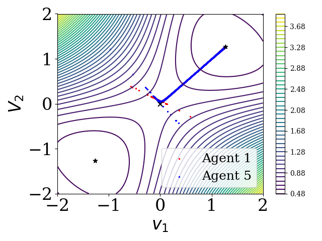
(a) Trajectory of $(\mathbf{v}_{1}^{k},\mathbf{V}_{2}^{k})$.

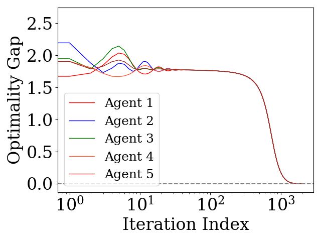
(b) Evolution of $\text{dist}(\mathbf{V}^{k},\mathcal{V}_{\tilde{L}}^{\star})$.

Figure 1: Second order properties of EXTRA for the non-convex inary classification example, where $\mathbf{V}^{k}=[\mathbf{v}_{1}^{k},\mathbf{V}_{2}^{k}]^{\top}$at each agent and $\mathcal{V}_{\tilde{L}}^{\star}$ denotes the set of local minimizers of $\tilde{L}$.

We investigate training a simple neural network for binary classification, serving as an example of non-convex distributed optimization. Given a dataset $(X,Y)$ where $X=\{x^{(1)},x^{(2)},\dots,x^{(m)}\}$ are the input features and $Y=\{y^{(1)},y^{(2)},\dots,y^{(m)}\}$ are the corresponding binary class labels, where $x^{(i)}\in\mathbb{R}^{n}$ and $y^{(i)}\in\{0,1\}$ for all $i=1,\dots,m$. As an instance of Problem (1), the learning problem with regularization term can be formulated as

$$\min_{\mathbf{v}_{1},\mathbf{V}_{2}}\tilde{L}(\mathbf{v}_{1},\mathbf{V}_{2})=\sum_{i=1}^{m}\tilde{L}_{i}(\mathbf{v}_{1},\mathbf{V}_{2}),$$

where $\tilde{L}_{i}(\mathbf{v}_{1},\mathbf{V}_{2})=\frac{1}{m}\ln(1+\exp(-\tilde{y}^{(i)}\mathbf{v}_{1}^{\top}\mathbf{V}_{2}x^{(i)}))+\frac{\eta}{2m}(\|\mathbf{v}_{1}\|^{2}+\|\mathbf{V}_{2}\|_{F}^{2})$, and for all $i=1,\dots,m$,

$$\tilde{y}^{(i)}=\begin{cases}-1,&\text{if}~y^{(i)}=0;\\ 1,&\text{if}~y^{(i)}=1.\end{cases}$$

For a straightforward visualization of the learning problem, we select parameters that render all variables as scalars, setting $n=d=1$. Consider that we engage $m=5$ agents to collaboratively solve this problem, connecting them in a regular graph with a degree of $2$. Note that each agent $i$ only knows its local objective $\tilde{L}_{i}(\mathbf{v}_{1},\mathbf{V}_{2})$. The figure shows the saddle point (marked by $*$) located at $(0,0)$, with the two local minimizers (marked by $\times$) symmetrically positioned in the positive and negative quadrants. In the following instance, we set $\eta=0.1$ and generate $\tilde{y}^{(i)}$ uniformly from $\{-1,1\}$ and $x^{(i)}\sim\mathcal{N}(\tilde{y}^{(i)},1)$. We choose mixing matrices satisfying Assumption II.4 and set step-size $\alpha=0.1$. All agents are initialized randomly near the stable manifold of the saddle point, $i.e.$, $\mathbf{v}_{1}+\mathbf{V}_{2}=0$. As shown in Fig. 1, since the initial iterates are near the stable manifold of the saddle point, EXTRA primarily perform a weighted averaging step. Afterwards, EXTRA successfully escapes the saddle point and converges to a local minimizer for all agents.

References

• [1] Stephen Boyd, Neal Parikh, Eric Chu, Borja Peleato, Jonathan Eckstein, etย al. Distributed optimization and statistical learning via the alternating direction method of multipliers. Foundations and Trendsยฎ in Machine learning, 3(1):1โ€“122, 2011.
• [2] Jakub Koneฤnแปณ, Brendan McMahan, and Daniel Ramage. Federated optimization: Distributed optimization beyond the datacenter. arXiv preprint arXiv:1511.03575, 2015.
• [3] Brendan McMahan, Eider Moore, Daniel Ramage, Seth Hampson, and Blaiseย Aguera yย Arcas. Communication-efficient learning of deep networks from decentralized data. In Artificial intelligence and statistics, pages 1273โ€“1282. PMLR, 2017.
• [4] Michael Rabbat and Robert Nowak. Distributed optimization in sensor networks. In Proceedings of the 3rd international symposium on Information processing in sensor networks, pages 20โ€“27, 2004.
• [5] Bjorn Johansson, Maben Rabi, and Mikael Johansson. A simple peer-to-peer algorithm for distributed optimization in sensor networks. In 2007 46th IEEE Conference on Decision and Control, pages 4705โ€“4710. IEEE, 2007.
• [6] Puย Wan and Michaelย D Lemmon. Event-triggered distributed optimization in sensor networks. In 2009 International Conference on Information Processing in Sensor Networks, pages 49โ€“60. IEEE, 2009.
• [7] Angelia Nediฤ‡ and Jiย Liu. Distributed optimization for control. Annual Review of Control, Robotics, and Autonomous Systems, 1:77โ€“103, 2018.
• [8] Danielย K Molzahn, Florian Dรถrfler, Henrik Sandberg, Stevenย H Low, Sambuddha Chakrabarti, Ross Baldick, and Javad Lavaei. A survey of distributed optimization and control algorithms for electric power systems. IEEE Transactions on Smart Grid, 8(6):2941โ€“2962, 2017.
• [9] Eduardo Camponogara and Heltonย F Scherer. Distributed optimization for model predictive control of linear dynamic networks with control-input and output constraints. IEEE Transactions on Automation Science and Engineering, 8(1):233โ€“242, 2010.
• [10] Angelia Nedic and Asuman Ozdaglar. Distributed subgradient methods for multi-agent optimization. IEEE Transactions on Automatic Control, 54(1):48โ€“61, 2009.
• [11] Angelia Nedic, Asuman Ozdaglar, and Pabloย A Parrilo. Constrained consensus and optimization in multi-agent networks. IEEE Transactions on Automatic Control, 55(4):922โ€“938, 2010.
• [12] Duลกan Jakovetiฤ‡, Joao Xavier, and Josรฉย MF Moura. Fast distributed gradient methods. IEEE Transactions on Automatic Control, 59(5):1131โ€“1146, 2014.
• [13] Annieย I Chen and Asuman Ozdaglar. A fast distributed proximal-gradient method. In 2012 50th Annual Allerton Conference on Communication, Control, and Computing (Allerton), pages 601โ€“608. IEEE, 2012.
• [14] Annie I-An Chen. Fast distributed first-order methods. PhD thesis, Massachusetts Institute of Technology, 2012.
• [15] Johnย C Duchi, Alekh Agarwal, and Martinย J Wainwright. Dual averaging for distributed optimization: Convergence analysis and network scaling. IEEE Transactions on Automatic control, 57(3):592โ€“606, 2011.
• [16] Wei Shi, Qing Ling, Gang Wu, and Wotao Yin. Extra: An exact first-order algorithm for decentralized consensus optimization. SIAM Journal on Optimization, 25(2):944โ€“966, 2015.
• [17] Angelia Nedic, Alex Olshevsky, and Wei Shi. Achieving geometric convergence for distributed optimization over time-varying graphs. SIAM Journal on Optimization, 27(4):2597โ€“2633, 2017.
• [18] Jinlong Lei, Han-Fu Chen, and Hai-Tao Fang. Primalโ€“dual algorithm for distributed constrained optimization. Systems & Control Letters, 96:110โ€“117, 2016.
• [19] Ran Xin and Usmanย A Khan. A linear algorithm for optimization over directed graphs with geometric convergence. IEEE Control Systems Letters, 2(3):315โ€“320, 2018.
• [20] Wei Shi, Qing Ling, Gang Wu, and Wotao Yin. A proximal gradient algorithm for decentralized composite optimization. IEEE Transactions on Signal Processing, 63(22):6013โ€“6023, 2015.
• [21] Mingyi Hong, Meisam Razaviyayn, and Jason Lee. Gradient primal-dual algorithm converges to second-order stationary solution for nonconvex distributed optimization over networks. In International Conference on Machine Learning, pages 2009โ€“2018. PMLR, 2018.
• [22] Amir Daneshmand, Gesualdo Scutari, and Vyacheslav Kungurtsev. Second-order guarantees of distributed gradient algorithms. SIAM Journal on Optimization, 30(4):3029โ€“3068, 2020.
• [23] Ioannis Panageas, Georgios Piliouras, and Xiao Wang. First-order methods almost always avoid saddle points: The case of vanishing step-sizes. Advances in Neural Information Processing Systems, 32, 2019.