Deep Learning-based OTFS Channel Estimation and Symbol Detection with Plug and Play Framework

Abstract

Orthogonal Time Frequency Space (OTFS) modulation has recently attracted significant interest due to its potential for enabling reliable communication in high-mobility environments. One of the challenges for OTFS receivers is the fractional Doppler that occurs in practical systems, resulting in decreased channel sparsity, and then inaccurate channel estimation and high-complexity equalization. In this paper, we propose a novel unsupervised deep learning (DL)-based OTFS channel estimation and symbol detection scheme, capable of handling different channel conditions, even in the presence of fractional Doppler. In particular, we design a unified plug-and-play (PnP) framework, which can jointly exploit the flexibility of optimization-based methods and utilize the powerful data-driven capability of DL. A lightweight Unet is integrated into the framework as a powerful implicit channel prior for channel estimation, leading to better exploitation of the channel sparsity and the characteristic of the noise simultaneously. Furthermore, to mitigate the channel estimation errors, we realize the PnP framework with a fully connected (FC) network for symbol detection at different noise levels, thereby enhancing robustness. Finally, numerical results demonstrate the effectiveness and robustness of the algorithm.

I Introduction

The forthcoming beyond 5G (B5G) wireless communication systems are envisioned to support a range of emerging high-mobility communication applications, such as low-earth-orbit satellites (LEOS), unmanned aerial vehicles (UAVs), and autonomous cars [1, 2]. The conventional long-term evolution (LTE) modulations such as orthogonal frequency-division multiplexing (OFDM) demonstrate limited capability in maintaining efficient and reliable communication performance under high-mobility channel conditions. This limitation primarily stems from the increased frequency dispersion induced by Doppler shift effects, which significantly degrades the system performance in such scenarios. To accommodate the heterogeneous demands of B5G wireless systems in high-mobility scenarios, researchers have proposed new modulation techniques and waveforms, e.g., orthogonal chirp division multiplexing (OCDM), affine frequency division multiplexing (AFDM), and orthogonal time frequency space (OTFS) modulations [3]. Amongst them, the recently proposed OTFS modulation has garnered significant interest due to its potential in enabling high-speed and ultra-reliable communications.

In high-mobility scenarios, wireless channels undergo dual dispersion effects in the time-frequency (TF) domain, where time dispersion arises from multipath propagation, while frequency dispersion is induced by Doppler shifts. Traditional OFDM modulation effectively mitigates inter-symbol interference (ISI) through cyclic prefix (CP) implementation. However, the inherent subcarrier orthogonality in OFDM systems is severely degraded by inter-carrier interference (ICI), ultimately leading to unsatisfactory reliability. In contrast to OFDM, OTFS modulation, grounded in Zak transform theory, operates in the delay-Doppler (DD) domain, exhibiting quasi-static, sparse, and compact channel characteristics [3]. Furthermore, each data symbol in the DD domain undergoes the whole channel fluctuation in the TF domain over an OTFS. The unique characteristic facilitates the full exploitation of channel diversity, which is essential for achieving the ultra-high reliability required by B5G wireless communication systems.

To fully harness the potential of OTFS modulation, recent works focus on the development of practical OTFS receiver implementations [4, 5]. A fundamental prerequisite for equalization is accurate channel estimation, which plays a vital role in ensuring reliable signal detection. Current channel estimation schemes mainly employ pilot-aided schemes to obtain the channel state information (CSI) at the receiver. In [6], the authors introduced an embedded pilot-aided channel estimation framework that utilizes a single pilot impulse accompanied by guard zero symbols in the DD domain, leveraging the inherent sparsity of the DD channel to enhance performance. To enhance the spectral efficiency, the authors of [7] develop a data-aided channel estimation algorithm, incorporating a superimposed pilot and data transmission scheme with an iterative process for channel estimation and data detection. In addition, the development of effective detection algorithms relying on accurate CSI is a crucial aspect of OTFS system implementation. Among the existing detection algorithms, the message-passing algorithm (MPA) based on factor graphs has been widely used for OTFS symbol detection [8]. Furthermore, an efficient implementation of the unitary approximate message passing (UAMP) detector was proposed in [9], where the structural properties of the OTFS channel matrix were exploited to enhance detection performance. However, due to the low-latency requirement, the Doppler resolution decreases since it depends on the OTFS block duration, leading to fractional Doppler effects, whereas wideband systems typically ensure adequate delay resolution. The presence of fractional Doppler shifts reduces channel sparsity, thereby severely impairing the effectiveness of conventional channel estimation algorithms [10]. Additionally, traditional symbol detection methods demonstrate diminished robustness in scenarios involving channel estimation errors, potentially leading to error propagation and subsequent detection performance deterioration [11]. These limitations motivate the exploration of data-driven approaches, which offer significant advantages by adaptively learning complicated channel characteristics from observed data, demonstrating superior robustness to estimation errors and environmental variations [12].

In the domain of wireless communications, deep learning (DL) has emerged as a transformative approach, demonstrating exceptional data-driven capabilities across various applications, including channel estimation, symbol detection, and spectrum sensing [13]. Specifically, a novel deep residual network was proposed in [14] for OTFS channel estimation. This approach effectively exploits the inherent sparsity characteristics of the channel, demonstrating enhanced estimation accuracy, particularly in challenging non-ideal transmission scenarios. Moreover, [15] developed a Viterbi-based neural network (ViterbiNet) for OTFS symbol detection, which achieves remarkable performance with minimal network size and training data requirements. Despite the superior performance of DL-based methods in addressing various communication tasks within wireless systems, they introduce significant challenges. One prominent challenge is the growing requirement for training and storing multiple neural network models, each designed for specific tasks. This not only results in substantial computational and storage expenses but also makes current DL-based solutions poorly scalable, especially for resource-constrained devices such as low-cost sensors and mobile platforms. Moreover, data-driven approaches often suffer from limited interpretability and rely on a large number of parameters to learn task-specific mappings, further heightening their inefficiency and complexity.

Fortunately, the plug-and-play (PnP) prior framework has emerged as a widely adopted solution to such challenges in the image reconstruction field, offering an integration of optimization-based flexibility and data-driven priors. In [16], a PnP prior framework with a trainable nonlinear reaction-diffusion denoiser was proposed to solve image deblurring problems. The authors in [17] utilized the PnP framework for hyperspectral image restoration, where an advanced image denoiser was developed using gated recurrent convolution structures along with both short- and long-range skip connections to effectively capture spatial dependencies. The proposed method achieves superior performance on super-resolution reconstruction, compressed sensing recovery, and inpainting tasks. These studies have successfully applied the PnP framework to manage various image reconstruction tasks, inspiring us to explore its potential application in wireless communication systems.

In this paper, we propose a PnP framework for addressing the challenges of channel estimation and symbol detection in OTFS. Specifically, we consider various OTFS channel conditions, including scenarios involving fractional and integer Doppler shifts. Furthermore, the PnP architecture demonstrates unique flexibility by integrating any pre-trained deep learning-based denoiser without requiring labeled datasets or extensive fine-tuning, thereby significantly reducing computational overhead.

The main contributions of this paper are summarized as follows:

• We introduce a deep PnP prior framework for OTFS receiver design that unifies channel estimation and symbol detection tasks. While these tasks are traditionally formulated as distinct optimization problems and typically tackled using different methodologies [11], our framework employs the variable splitting technique to decompose various optimization problems into model-based subproblems with a shared denoising component. This common denoising subproblem is efficiently resolved using a DL-based denoiser, providing a coherent solution for OTFS receiver design.

• To implement the proposed framework, we utilize a lightweight Unet-based denoiser to facilitate the Unet-based PnP (UPnP) method for channel estimation, where the encoder-decoder structure is specifically designed to exploit spatial features of noisy channel matrices and additive noise characteristics, simultaneously. Inheriting from the feature extraction and adaptability, the proposed UPnP could further improve the estimation accuracy and extend to different channel conditions without additional training.

• To accomplish the symbol detection task, we employ a fully connected (FC) neural network to construct an FC-based PnP (FPnP) framework for symbol detection. This approach leverages the constellation prior knowledge to refine the model-based de-correlation results, thereby mitigating noise and interference. To further improve computational efficiency, we perform the de-correlation operation in the time domain rather than in the DD domain, effectively reducing the overall complexity while preserving performance. Therefore, the FPnP method can improve detection accuracy under imperfect channel estimation conditions and enhance robustness against channel impairments.

• Extensive simulations have been performed to verify the effectiveness of the proposed method in channel estimation and symbol detection, respectively. The results highlight the scalability of the approach, demonstrating robust channel estimation performance across both integer and fractional Doppler cases. Moreover, the PnP-based symbol detection method significantly improves detection accuracy under non-ideal channel conditions.

The remainder of this work is organized as follows. Section II presents the system model for OTFS modulation, along with the input-output relationship with bi-orthogonal and rectangular waveforms. Section III formulates the problems of channel estimation and symbol detection. Section IV presents the design of a unified deep PnP framework for the OTFS receiver. As an implementation of the proposed framework, Section V introduces a UPnP algorithm for channel estimation and an FPnP algorithm for symbol detection. To evaluate the effectiveness of the proposed approach, extensive simulation results are provided in Section VI. Finally, the key findings of this work are summarized in VII.

Notations: The following notations are used in this work. Scalars, vectors, and matrices are denoted by regular font (i.e., $x$), bold lowercase letters (i.e., $\mathbf{x}$), and bold uppercase letters (i.e., $\mathbf{X}$), respectively. The sets $\mathbb{C}^{M\times N}$ and $\mathbb{R}^{M\times N}$ represent complex-valued matrices and real-valued matrices of size $M\times N$, respectively. The symbols $\Re(\cdot)$ and $\Im(\cdot)$ represent the real and imaginary components of an input complex number. The real-valued Gaussian distribution and the circularly symmetric complex Gaussian (CSCG) distribution are represented by $\mathcal{N}(\boldsymbol{\mu},\boldsymbol{\Sigma})$ and $\mathcal{C}\mathcal{N}(\boldsymbol{\mu},\boldsymbol{\Sigma})$, where $\boldsymbol{\mu}$ and $\boldsymbol{\Sigma}$ denote the mean vector and the covariance matrix, respectively. The notation $\mathbf{I}_{N}$ is the identity matrix of size $N\times N$, and $\mathbf{1}_{N}$ is the column vector of all ones with size $N\times 1$. $(\cdot)^{T}$, $(\cdot)^{H}$, and $(\cdot)^{*}$ stand for transpose, Hermitian transpose, and conjugate operations, respectively. The notation $O(\cdot)$ represents the order of computational complexity.

II System Model

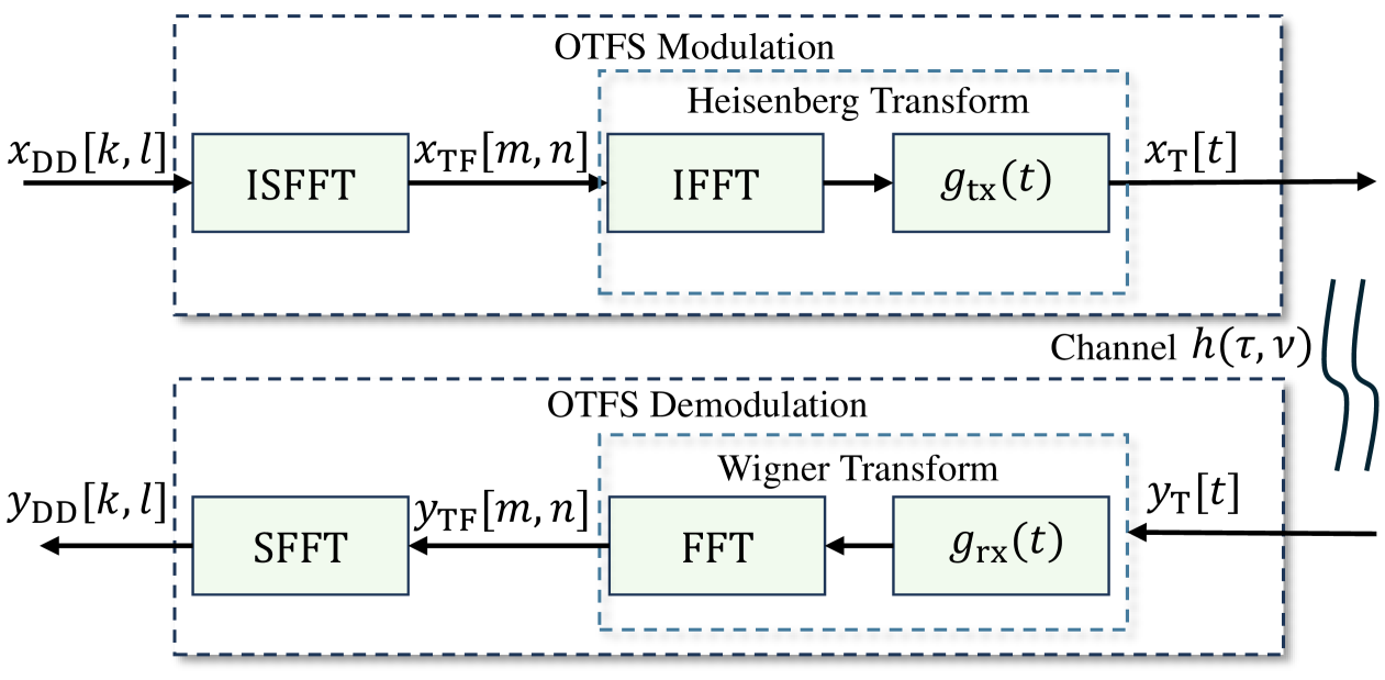
Figure 1: Block diagram of the considered OTFS system.

II-A OTFS Modulation

We consider an OTFS modulation as shown in Fig. 1. Let $N$ denote the number of time slots and $M$ the number of sub-carriers for each OTFS symbol. The information symbols $x_{\mathrm{DD}}[k,l]$, with Doppler index $k\in\{0,\cdots,N-1\}$ and delay index $l\in\{0,\cdots,M-1\}$, are selected from a constellation set $\mathbb{Q}=\{x_{1},\cdots,x_{q^{\prime}}\}$ of size $q^{\prime}$ and are placed in the DD domain. The TF domain transmitted symbol $x_{\mathrm{TF}}[n,m]$, with time index $n\in\{0,\dots,N-1\}$ and frequency index $m\in\{0,\dots,M-1\}$, is obtained through the inverse symplectic finite Fourier transform (ISFFT)., i.e.,

$$x_{\mathrm{TF}}\left[n,m\right]=\frac{1}{\sqrt{NM}}\sum_{k=0}^{N-1}\sum_{l=0}^{M-1}x_{\mathrm{DD}}\left[k,l\right]e^{j2\pi\left(\frac{nk}{N}-\frac{ml}{M}\right)}.$$ (1)

The time domain transmitted OTFS signal $x_{\mathrm{T}}(t)$ is derived from

$$x_{\mathrm{T}}(t)=\sum_{n=0}^{N-1}\sum_{m=0}^{M-1}x_{\mathrm{TF}}[n,m]g_{\mathrm{tx}}(t-nT)e^{j2\pi m\Delta f(t-nT)},$$ (2)

where $T$ and $\Delta f$ are the TF domain time slot duration and sub-carriers spacing, respectively. The notation $g_{\mathrm{tx}}(t)$ denotes the pulse shaping filter. We consider the OTFS signal transmitting over a time-varying channel, whose impulse response can be characterized with DD domain representation as

$$h(\tau,\nu)=\sum_{i=1}^{P}h_{i}\delta(\tau-\tau_{i})\delta(\nu-\nu_{i}),$$ (3)

where $P$ is the number of paths, and $h_{i}$, $\tau_{i}$ and $\nu_{i}$ denote the channel coefficients, delay, and Doppler shifts corresponding to the $i$-th path, respectively. Specifically, the delay shifts $\tau_{i}$ and Doppler shifts $\nu_{i}$ associated with the $i$-th path can be expressed as

$$\tau_{i}=\frac{l_{i}}{M\Delta f},\nu_{i}=\frac{k_{i}+\kappa_{i}}{NT}.$$ (4)

Here, integers $l_{i}\in[0,l_{\max}]$ and $k_{i}\in[-k_{\max},k_{\max}]$ are delay and Doppler indices corresponding to the $i$-th path, where $l_{\max}$ and $k_{\max}$ denote maximum delay and Doppler index, respectively. $\kappa_{i}\in[-\frac{1}{2},\frac{1}{2}]$ is fractional Doppler shifts from nearest Doppler. The terms $\frac{1}{M\Delta f}$ and $\frac{1}{NT}$ represent the delay and Doppler resolutions, respectively. It is noteworthy that the sampling time $\frac{1}{M\Delta f}$ generally assumes a sufficiently small value, then the effects of fractional delays can be disregarded in typical wide-band systems [18].

At the receiver side, the received symbols in the DD domain can be obtained via

$$y_{\mathrm{DD}}[k,l]=\frac{1}{\sqrt{NM}}\sum_{n=0}^{N-1}\sum_{m=0}^{M-1}y_{\mathrm{TF}}[m,n]e^{-j2\pi(\frac{nk}{N}-\frac{ml}{M})},$$ (5)

where $y_{\mathrm{TF}}[m,n]$ denotes the received symbol in the discrete-TF domain.

II-B Input-Output Relationship Based on Bi-orthogonal Waveform

In this section, we first consider that the transmit and receive pulse shaping waveforms satisfy the bi-orthogonal property. Therefore, the input-output relationship without the noise term in the DD domain can be written as [3]

$$y_{\mathrm{DD}}[k,l] =\frac{1}{NM}\sum_{k^{\prime}=0}^{N-1}\sum_{l^{\prime}=0}^{M-1}h_{w}[k^{\prime},l^{\prime}]x_{\mathrm{DD}}[k-k^{\prime},l-l^{\prime}].$$ (6)

Here $h_{w}[\cdot,\cdot]$ denotes the sampled version of the impulse response function, which is given by

$$h_{w}[k^{\prime},l^{\prime}]=h_{w}(\nu,\tau)|_{\nu=\frac{k^{\prime}}{NT},\tau=\frac{l^{\prime}}{M\Delta f}}.$$ (7)

Here, $h_{w}(\nu,\tau)$ is the circular convolution of the channel response with the SFFT of a rectangular windowing function in the TF domain, which is given by

$$h_{w}(\nu,\tau)=\int\int h(\tau^{\prime},\nu^{\prime})w(\nu-\nu^{\prime},\tau-\tau^{\prime})e^{-j2\pi\nu\tau}d\tau^{\prime}d\nu^{\prime},$$ (8)

with

$$w(\nu,\tau)=\sum_{n=0}^{N-1}\sum_{m=0}^{M-1}e^{-j2\pi(\nu nT-\tau m\Delta f)}.$$ (9)

By substituting (3) into (8), we obtain that

$$h_{w}(\nu,\tau) =\sum_{i=1}^{P}h_{i}e^{-j2\pi\nu_{i}\tau_{i}}w(\nu-\nu_{i},\tau-\tau_{i})$$

$$=\sum_{i=1}^{P}h_{i}e^{-j2\pi\nu_{i}\tau_{i}}g_{1}(\tau,\tau_{i})g_{2}(\nu,\nu_{i}),$$ (10)

where $g_{1}(\tau,\tau_{i})\triangleq\sum_{m^{\prime}=0}^{M-1}e^{j2\pi(\tau-\tau_{i})m^{\prime}\Delta f}$, $g_{2}(\nu,\nu_{i})\triangleq\sum_{n^{\prime}=0}^{N-1}e^{-j2\pi(\nu-\nu_{i})n^{\prime}T}$. Let us analyze $g_{1}(\tau,\tau_{i})$ with sampled version as

$$g_{1}(\tau,\tau_{i})|_{\tau=\frac{l^{\prime}}{M\Delta f}}=\sum_{m^{\prime}=0}^{M-1}e^{j\frac{2\pi}{M}(l^{\prime}-l_{i})m^{\prime}}=\frac{e^{j2\pi(l^{\prime}-l_{i})}-1}{e^{j\frac{2\pi}{M}(l^{\prime}-l_{i})}-1}.$$ (11)

It can be observed that $g_{1}(\frac{l^{\prime}}{M\Delta f},\tau_{i})=M$, for $[l^{\prime}-l_{i}]_{M}=0$, and $g_{1}(\frac{l^{\prime}}{M\Delta f},\tau_{i})=0$ for the rest $[l^{\prime}-l_{i}]_{M}$. Similarly, the sampled version of $g_{2}(\nu,\nu_{i})$ is given by

$$g_{2}(\frac{k^{\prime}}{NT},\nu_{i})=\frac{e^{j2\pi(k^{\prime}-k_{i}-\kappa_{i})}-1}{e^{j\frac{2\pi}{N}(k^{\prime}-k_{i}-\kappa_{i})}-1}.$$ (12)

The magnitude of $\frac{1}{N}g_{2}(\frac{k^{\prime}}{NT},\nu_{i})$ is given by

$$\left|\frac{1}{N}g_{2}(\frac{k^{\prime}}{NT},\nu_{i})\right|=\left|\frac{\sin(\pi(k^{\prime}-k_{i}-\kappa_{i}))}{N\sin(\frac{\pi}{N}(k^{\prime}-k_{i}-\kappa_{i}))}\right|.$$ (13)

As stated in [10], the magnitude decreases rapidly with slope of ${\pi}(k^{\prime}-k_{i}-\kappa_{i})$. Here, we only consider $2N_{i}+1$ spread numbers around the peak $k_{i}$, i.e., $[k_{i}-N_{i}]_{M}\leq k^{\prime}\leq[k_{i}+N_{i}]_{M}$, where $N_{i}$, $N_{i}\ll N$, denotes the truncated number indicating the parts that contain most of the energy. According to the approximation, the effective channel can be written as

$$h_{w}[k^{\prime},l^{\prime}]\approx \sum_{i=1}^{P}\sum_{q=-N_{i}}^{N_{i}}h_{i}e^{-j2\pi\nu_{i}\tau_{i}}g_{1}(\frac{l^{\prime}}{M\Delta f},\tau_{i})$$

$$g_{2}(\frac{k^{\prime}}{NT},\nu_{i})\delta(k^{\prime}-k_{i}-q).$$ (14)

Let us analyze the sparsity of $h_{w}[k^{\prime},l^{\prime}]$ under different channel conditions. In the scenario of integer delay and Doppler integer delay and Doppler, i.e., $\kappa_{i}=0$, the magnitude of $h_{w}[k^{\prime},l^{\prime}]$ can be expressed as

$$h_{w}[k^{\prime},l^{\prime}]=\sum_{i=1}^{P}h_{i}e^{-j2\pi\nu_{i}\tau_{i}}\delta(l^{\prime}-l_{i})\delta(k^{\prime}-k_{i}).$$ (15)

The channel response is completely sparse in the DD domain, as depicted in Fig. 2 (a), enabling efficient signal processing in this domain. In this case, the channel prior can be represented using the $\ell_{1}$-norm. In the scenario of fractional Doppler, the magnitude of $g_{2}(\nu,\nu_{i})$ is given by (13). As shown in Fig. 2 (b), it can be observed that the sparsity decreases when the Doppler spread is large since signals are not compressed in the Doppler domain [19]. It is noteworthy that the degree of expansion is significantly influenced by the absolute value of $\kappa_{i}$. The sparsity of the channel can also be influenced by other variables, such as the number of paths $P$, as shown in Fig. 2 (c). In the latter two cases, the channel exhibits block sparsity, making it challenging to effectively capture the channel priors using only the $\ell_{1}$ norm. Therefore, the input-output relationship in the DD domain can be written as [20]

$$y_{\mathrm{DD}}[k,l]=\sum_{i=0}^{P} \sum_{q=-N_{i}}^{N_{i}}h_{i}e^{-j2\pi\frac{\tau_{i}\nu_{i}}{MN}}\eta(q,\kappa_{i})$$

$$x_{\mathrm{DD}}[[k-k_{i}+q]_{N},[l-l_{i}]_{M}]+v_{\mathrm{DD}}[k,l],$$ (16)

where $\eta(q,\kappa_{i})=\frac{1-e^{-j2\pi(-q-\kappa_{i})}}{N-Ne^{-j\frac{2\pi}{N}(-q-\kappa_{i})}}$. The term $v_{\mathrm{DD}}[k,l]$ denotes the Gaussian noise in the DD domain.

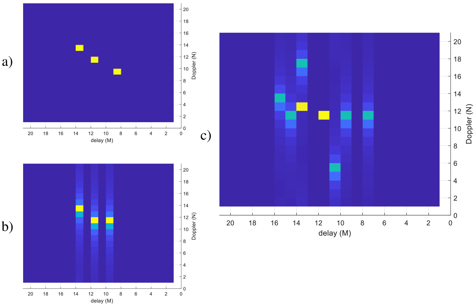
Figure 2: Different priors of OTFS channels due to different channel parameters, illustrating burst sparsity and block sparsity.

III Problem Formulation

III-A Problem Formulation for Channel Estimation

In this paper, the pilot scheme in [5] is adopted, where pilot symbols are placed in the DD domain, surrounded by guard space. As depicted in Fig. 3, the lengths of pilots along the delay and Doppler are $P_{m}$ and $P_{n}$, respectively. It is noteworthy that the deployment of multiple pilots can reduce the peak-to-average power ratio (PAPR) [9], albeit with a slight trade-off in spectral efficiency. To mitigate interference between pilots and symbols, the length of guard intervals should be $\bar{P}_{m}\geq(l_{\max}+1)$ and $\bar{P}_{n}\geq 2\hat{k}_{\max}+1$, with $\hat{k}_{\max}$ being $k_{\max}+N_{i}$.

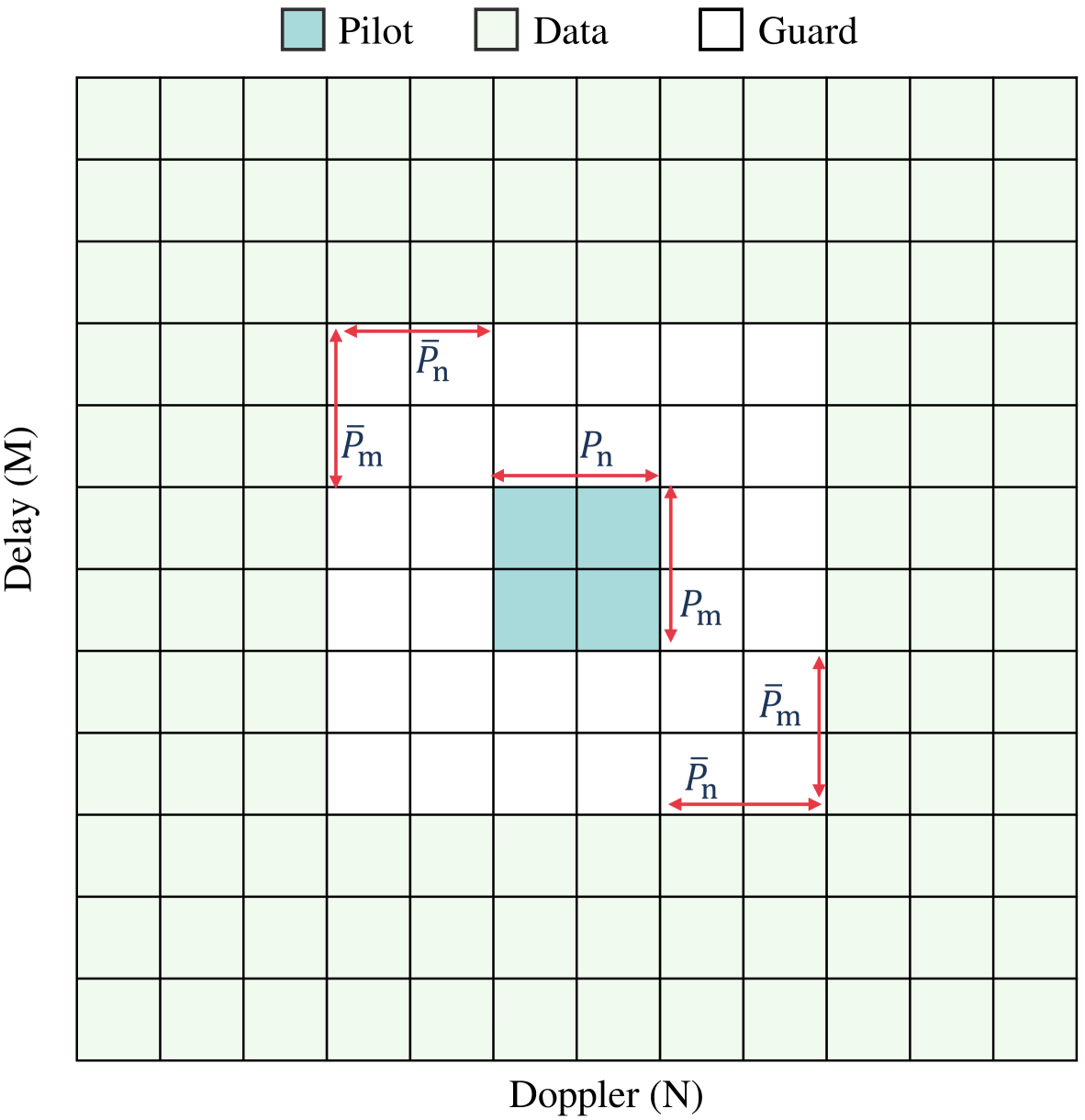
Figure 3: The considered OTFS pilot placement scheme, showing pilots in the DD domain surrounded by guarding interval with zeros.

Note that an ideal bi-orthogonal is impractical due to the constraints imposed by Heisenberg’s uncertainty principle [21]. Therefore, we employ a rectangular transmit and receive waveform. Based on this, the input-output relationship can be expressed as [20]

$$y_{\mathrm{DD}}[k,l] =\sum_{i=1}^{P}\sum_{q=-N_{i}}^{N_{i}}h_{i}e^{j2\pi\left(\frac{l-l_{i}}{M}\right)\left(\frac{k_{i}+\kappa_{i}}{N}\right)}\alpha_{i}(k,l,q)$$

$$\times x_{\mathrm{DD}}[[k-k_{i}+q]_{N},[l-l_{i}]_{M}]+\tilde{n}[k,l],$$ (17)

where

$$\alpha_{i}(k,l,q)=\begin{cases}\eta(q,\kappa_{i})&l_{i}\leq l<M,\\ (\eta(q,\kappa_{i})-\frac{1}{N})e^{-j2\pi\frac{[k-k_{i}+q]_{N}}{N}}&0\leq l<l_{i},\end{cases}$$ (18)

Based on the employed pilot placement scheme, we place the pilot symbols to ensure that their index satisfies $l\geq l_{\max}$, then (17) can be rewritten as

$$y_{\mathrm{DD}}[k,l] =\sum_{i=1}^{P}\sum_{q=-N_{i}}^{N_{i}}h_{i}\eta(q,\kappa_{i})e^{j2\pi\frac{(l-l_{i})(k_{i}+\kappa_{i})}{MN}}$$

$$\times x_{\mathrm{DD}}\left[[k-k_{i}+q]_{N},[l-l_{i}]_{M}\right]+\bar{n}[k,l].$$ (19)

For an arbitrary form of the DD domain signal model, e.g., (19), here, we can rewrite it in a matrix form as

$$\mathbf{y}_{\mathrm{DD}}=\boldsymbol{\Phi}_{\mathrm{DD}}\mathbf{h}+\bar{\mathbf{n}}_{\mathrm{DD}},$$ (20)

where $\mathbf{y}_{\mathrm{DD}}\in,\bar{\mathbf{n}}_{\mathrm{DD}}\in\mathbb{C}^{L_{m}\times 1}$ with $L_{m}=(P_{m}+l_{\max}+1)(P_{n}+2\hat{k}_{\max}+1)$, $L_{n}=(l_{\max}+1)(2\hat{k}_{\max}+1)$. The measurement matrix $\boldsymbol{\Phi}_{\mathrm{DD}}\in\mathbb{C}^{L_{m}\times L_{n}}$ is derived from the pilot symbols with the $(k_{i}\,j_{i})$-st row is given by $\left[\mathbf{x}_{\mathrm{DD}}[k_{i}:k_{i}-2\hat{k}_{\max},\,j_{i}:j_{i}-l_{\max}]\right]$, where $k_{i}\in\{0:P_{n}+2\hat{k}_{\max}\}$ and $j_{i}\in\{0:P_{m}+l_{\max}\}$. Since the additional phase term $e^{j2\pi\frac{l(k_{i}+\kappa_{i})}{MN}}$ in (19) is related to both the channel and data, and $\mathbf{h}$ cannot be directly recovered when the measurement matrix $\boldsymbol{\Phi}_{\mathrm{DD}}$ contains unknown parameters, we neglect the additional phase difference with minimal performance degradation, as mentioned in [22]. The term $\mathbf{h}\in\mathbb{C}^{L_{n}\times 1}$ can be inversely vectorized to obtain a truncated 2-dimension (2D) DD channel $\mathcal{H}\in\mathbb{C}^{(l_{\max}+1)\times(2\hat{k}_{\max}+1)}$. It is noteworthy the truncated DD channel $\mathcal{H}$ has finite supports $[-\hat{k}_{\max}:\hat{k}_{\max}]$ along the Doppler dimension and $[0:l_{\max}]$ along delay dimension, as specified in (14). For the vector $\mathbf{h}=[h_{1},\cdots,h_{L_{n}}]$, the support set of $\mathbf{h}$ is defined as $\mathrm{supp}(\mathbf{h})=\{i:h_{i}\neq 0\}$, and $\mathbf{h}$ is $\gamma$-sparse if $\left|\mathrm{supp}(\mathbf{h})\right|\leq\gamma$.

As discussed earlier, the sparsity $\gamma$ varies due to the fractional spread and the increase in the number of paths. Traditionally, specific priors are required for algorithm design in different scenarios, such as the hidden Markov model (HMM) for message passing-based methods and 1-norm priors for sparse Bayesian algorithms [14, 23]. Leveraging the powerful capabilities of deep learning, we propose a unified PnP framework with a deep denoiser prior to address the channel estimation issue, thereby enhancing scalability.

III-B Formulation of Symbol Detection

To formulate the symbol detection problem, we derive the matrix form of the effective channels in the TF domain and the DD domain. Let $\mathbf{x}_{\mathrm{DD}}$ denote the 1D vector form of $\mathbf{X}_{\mathrm{DD}}\in\mathbb{Q}^{M\times N}$ obtained by column-wise rearrangement, i.e., $\mathbf{x}_{\mathrm{DD}}=\mathrm{vec}(\mathbf{X}_{\mathrm{DD}})$, where the $(k,l)$-th element $x_{\mathrm{DD}}[k,l]$ represents the DD information symbols. Similarly, $\mathbf{y}_{\mathrm{DD}}$ denotes the vector form of received symbols in the DD domain, $\mathbf{x}_{\mathrm{T}}$ is the transmitted vector in the time domain, and $\mathbf{y}_{\mathrm{T}}$ is the vector at the received side in the time domain. We utilize zero padding (ZP) to implement the OTFS system with a padding length $L_{\mathrm{zp}}\geq l_{\max}$. After removing the ZP, the time domain input-output relation can be written as [18]

$$\mathbf{y}_{\mathrm{T}}=\mathbf{H}_{\mathrm{T}}\mathbf{x}_{\mathrm{T}}+\mathbf{n}_{\mathrm{T}},$$ (21)

where $\mathbf{n}_{\mathrm{T}}$ denotes the noise in the time domain. The effective channel in the time domain is a block diagonal matrix and given by $\mathrm{diag\{\mathbf{H}_{1},\cdots,\mathbf{H}_{n},\cdots,\mathbf{H}_{N}\}}$, where $\mathbf{H}_{n}\in\mathbb{C}^{M\times M}$ with $n\in[1,N]$ is the $n$-th sub-block effective channel matrix in the time domain. With the FFT and SFFT operations, an equivalent vectorization form in the DD domain is given by [18]

$$\mathbf{y}_{\mathrm{DD}}=\mathbf{H}_{\mathrm{DD}}\mathbf{x}_{\mathrm{DD}}+\mathbf{n}_{\mathrm{DD}},$$ (22)

where $\mathbf{n}_{\mathrm{DD}}\in\mathbb{C}^{MN}$ denotes the noise vector with each element following distribution $\mathcal{CN}(0,\sigma^{2}_{\mathrm{d}})$ and $\mathbf{H}_{\mathrm{DD}}\in\mathbb{C}^{MN\times MN}$ is the effective channel matrix in the DD domain, which is given by

$$\mathbf{H}_{\mathrm{DD}}=\left(\mathbf{F}_{N}\otimes\mathrm{G}_{\mathrm{rx}}\right)\mathbf{H}_{\mathrm{T}}\left(\mathbf{F}_{N}^{\mathrm{H}}\otimes\mathrm{G}_{\mathrm{tx}}\right).$$ (23)

In (23), the notations $\mathrm{G}_{\mathrm{tx}}=\mathrm{G}_{\mathrm{rx}}=\mathbf{I}_{\mathrm{M}}$ represent the matrix forms of the transmit and receive pulse shaping waveforms, respectively. To address the symbol detection problem, we combine an FC neural network for the PnP framework with a model-based time-domain equalization method to reduce computational complexity.

IV Deep Learning-Based PnP Framework

In this section, we present a PnP framework that leverages DL-based approaches for OTFS receiver design. In the developed PnP framework, the linear inverse problems, i.e., channel estimation and symbol detection, such as (20) and (22), can be solved by alternately updating the estimated parameters using a combination of matrix computation methods and a DL-based approach. In the following, we introduce the proposed PnP framework for the OTFS receiver.

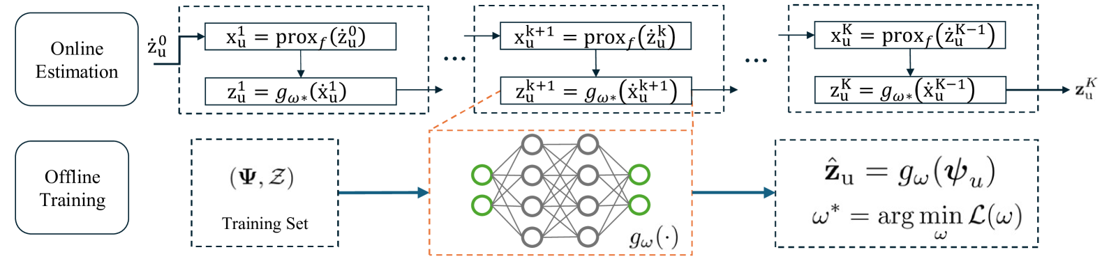
Figure 4: Illustration of the proposed PnP framework based on deep learning.

IV-A The Unified Framework for OTFS Receivers

Assuming a general linear problem, and the observed data is given by

$$\mathbf{y}_{\mathrm{u}}=\boldsymbol{\Phi}_{\mathrm{u}}\mathbf{x}_{\mathrm{u}}+\mathbf{n}_{\mathrm{u}},$$ (24)

where $\boldsymbol{\Phi}_{\mathrm{u}}\ \in\mathbb{C}^{a\times b}$ is the measurement matrix, and $\mathbf{n}_{\mathrm{u}}\in\mathbb{C}^{a\times 1}$ is a complex Gaussian noise vector. Here, $a$ and $b$ are arbitrary positive integers. A prior knowledge of the unknown vector $\mathbf{x}_{\mathrm{u}}$, such as a detailed function representing the sparsity of $\mathbf{x}_{\mathrm{u}}$, is denoted by $\mathcal{J}(\mathbf{x}_{\mathrm{u}})$. The objective is to recover $\mathbf{x}_{\mathrm{u}}$, which can be achieved by addressing the following problem, i.e.,

$$\min_{\mathbf{x}_{\mathrm{u}}}\frac{1}{2}||\mathbf{y}_{\mathrm{u}}-\boldsymbol{\Phi}_{\mathrm{u}}\mathbf{x}_{\mathrm{u}}||^{2}+\lambda\mathcal{J}(\mathbf{x}_{\mathrm{u}}),$$ (25)

where $\lambda\gg 0$ is a regularization parameter that determines the influence of the regularization term.

Proximal algorithms are frequently employed to address optimization problems of the form presented in Eq. (25), particularly when the function $\mathcal{J}(\cdot)$ is nonsmooth. The flexible deep PnP framework is grounded in the alternating direction method of multipliers (ADMM) that has gained substantial attention in recent years for its efficiency in handling proximal optimization problems [24]. The core concept of the deep PnP approach lies in decoupling the prior term and the data-fidelity term into two distinct subproblems, where the subproblem related to the prior can be interpreted as a denoising task that can be addressed using a pre-trained denoiser. This design not only preserves the flexibility to tackle signal restoration problems within a unified framework but also capitalizes on the robust prior-modeling capabilities offered by deep neural networks (DNNs). Specifically, the deep PnP method solves problem (25) by introducing an auxiliary variable $\mathbf{z}_{\mathrm{u}}$ as

$$\min_{\mathbf{{x}_{\mathrm{u}}}}\quad \frac{1}{2}\left\|\mathbf{\mathbf{y}_{\mathrm{u}}}-\boldsymbol{\Phi}_{\mathrm{u}}\mathbf{x}_{\mathrm{u}}\right\|_{2}^{2}+\lambda\mathcal{J}(\mathbf{z}_{\mathrm{u}})$$

$$s.t.\quad \mathbf{z}_{\mathrm{u}}=\mathbf{x}_{\mathrm{u}}.$$ (26)

Then we rewrite (26) by forming augmented Lagrangian function as

$$\mathcal{L}_{\rho}\left(\mathbf{x}_{\mathrm{u}},\mathbf{z}_{\mathrm{u}},\mathbf{u}_{\mathrm{u}}\right)= \frac{1}{2}\left\|\mathbf{y}_{\mathrm{u}}-\boldsymbol{\Phi}_{\mathrm{u}}\mathbf{x}_{\mathrm{u}}\right\|_{2}^{2}+\lambda\mathcal{J}\left(\mathbf{z}_{\mathrm{u}}\right)$$

$$+\frac{\rho}{2}\left\|\mathbf{x}_{\mathrm{u}}-\mathbf{z}_{\mathrm{u}}\right\|_{2}^{2}+\mathbf{u}_{\mathrm{u}}^{T}\left(\mathbf{x}_{\mathrm{u}}-\mathbf{z}_{\mathrm{u}}\right),$$ (27)

where $\rho\gg 0$ is a penalty parameter and $\mathbf{u}_{\mathrm{u}}$ is the dual variable of $\mathbf{z}_{\mathrm{u}}$. It is noteworthy that parameters $\rho$ and $\lambda$ play a crucial role in the entire alternating iterative optimization process, significantly affecting its convergence. To ensure that $\mathbf{x}_{\mathrm{u}}$ and $\mathbf{z}_{\mathrm{u}}$ converge to a fixed point, the value of $\rho$, which represents the weight of the constraint term, must progressively increase during the iterative process [25]. Optimization problem (27) can be solved by iteratively solving the following three subproblems with variables $\mathbf{z}_{\mathrm{u}}$, $\mathbf{x}_{\mathrm{u}}$ and $\mathbf{u}_{\mathrm{u}}$ in turn, which is expressed as

$$\mathbf{x}_{\mathrm{u}}^{k+1}=\arg\min_{\mathbf{x}_{\mathrm{u}}}f(\mathbf{x}_{\mathrm{u}})+\frac{\rho}{2}\left\|\mathbf{x}_{\mathrm{u}}-\mathbf{\dot{z}}_{\mathrm{u}}^{k}\right\|_{2}^{2},$$ (28)

$$\mathbf{z}_{\mathrm{u}}^{k+1}=\arg\min_{\mathbf{z}_{\mathrm{u}}}\mathcal{J}\left(\mathbf{z}_{\mathrm{u}}\right)+\frac{1}{2\sigma^{2}}\left\|\mathbf{z}_{\mathrm{u}}-\mathbf{\dot{x}}_{\mathrm{u}}^{k+1}\right\|_{2}^{2},$$ (29)

$$\mathbf{u}_{\mathrm{u}}^{k+1}=\mathbf{u}_{\mathrm{u}}^{k}+(\mathbf{x}_{\mathrm{u}}^{k+1}-\mathbf{z}_{\mathrm{u}}^{k+1}),$$ (30)

where $f(\mathbf{x}_{\mathrm{u}})=\frac{1}{2}\left\|\mathbf{y}_{\mathrm{u}}-\boldsymbol{\Phi}_{\mathrm{u}}\mathbf{x}_{\mathrm{u}}\right\|_{2}^{2}$, $\mathbf{\dot{z}}_{\mathrm{u}}^{k}=\mathbf{z}_{\mathrm{u}}^{k}-\mathbf{u}_{\mathrm{u}}^{k}$, $\mathbf{\dot{x}}_{\mathrm{u}}^{k+1}=\mathbf{x}_{\mathrm{u}}^{k+1}+\mathbf{u}_{\mathrm{u}}^{k}$, and $\sigma^{2}=\lambda/2\rho$. As shown in Fig. 4, the developed deep PnP framework consists of two update methods: a model-based method is employed to solve (28), while a DL-based method is utilized to solve (29).

Update $\mathbf{x}_{\mathrm{u}}^{k+1}$: For the subproblem (28), we can derive the closed-form solution via a least squire (LS) method, i.e.,

$$\mathbf{x}_{\mathrm{u}}^{k+1} =(\boldsymbol{\Phi}_{\mathrm{u}}^{H}\boldsymbol{\Phi}_{\mathrm{u}}+\rho\,\mathbf{I})^{-1}(\boldsymbol{\Phi}_{\mathrm{u}}^{H}\mathbf{y}_{\mathrm{u}}+\rho\,\mathbf{\dot{z}}_{\mathrm{u}}^{k}).$$ (31)

It is noteworthy that solution (31) can be simplified with the specific measurement matrix $\boldsymbol{\Phi}_{\mathrm{u}}$. For instance, when the channel experiences flat fading, the $\boldsymbol{\Phi}_{\mathrm{u}}$ served as the channel matrix in the frequency domain is a circulant matrix, and the model-based update step for the symbol detection problem can be implemented with element-wise division [25].

Update $\mathbf{z}_{\mathrm{u}}^{k+1}$: Given a function $f^{\prime}(x)$ and penalty factor $\lambda^{\prime}$, the proximal mapping function is defined as

$$\mathrm{prox}_{f^{\prime}}(\mathbf{z})=\arg\min_{\mathbf{x}}\{f^{\prime}(\mathbf{x})+\frac{1}{2}\lambda^{\prime}\left\|\mathbf{x}-\mathbf{z}\right\|^{2}\},$$ (32)

which is well defined if $f^{\prime}(\cdot)$ is proper, closed, and convex. Accordingly, subproblem (29) can be expressed with proximal mapping function as $\mathbf{z}_{\mathrm{u}}^{k+1}=\mathrm{prox}_{\mathcal{J}}(\mathbf{\dot{x}}_{\mathrm{u}}^{k+1})$. In particular, the proximal function can be reformulated with MAP estimation as

$$\mathbf{z}_{\mathrm{u}}^{k+1} =\arg\max_{\mathbf{z}_{\mathrm{u}}}p(\mathbf{\dot{x}}_{\mathrm{u}}^{k+1}|\mathbf{z}_{\mathrm{u}})$$

$$=\arg\min_{\mathbf{z}_{\mathrm{u}}}\left(-\log p(\mathbf{z}_{\mathrm{u}}|\mathbf{\dot{x}}_{\mathrm{u}}^{k+1})-\log p(\mathbf{z}_{\mathrm{u}})\right),$$ (33)

where $p(\cdot)$ represents the probability density function (pdf). Comparing (33) and (29), we conclude that the step of updating $\mathbf{z}_{\mathrm{u}}^{k+1}$ could be interpreted as a Gaussian denoising problem, where $\sigma^{2}$ denotes the noise variance, $\mathbf{z}_{\mathrm{u}}^{k+1}$ is the “denoised” signal, and $\mathbf{\dot{x}}_{\mathrm{u}}^{k+1}$ is the noisy signal. Nevertheless, solving this problem is challenging as it requires explicit knowledge of the prior $\mathcal{J}(\mathbf{z}_{\mathrm{u}})$, i.e., $p(\mathbf{z}_{\mathrm{u}})$, and even with a good approximation, it remains extremely difficult to carry out analytically. Furthermore, the parameter $\rho$ increases during the iterative process, implying that the noise variance $\sigma^{2}$ changes continuously. Thus, a practical data-driven denoiser that can handle varying noise levels and complicated prior knowledge of estimated signals is essential for the efficient deployment of the PnP framework.

IV-B Offline Pre-Training for the Denoiser

Fig. 4 illustrates the two stages of the proposed approach: online estimation and offline training. We can acquire the following set for offline training as

$$(\boldsymbol{\Psi},\mathcal{Z})=\{(\boldsymbol{\psi}_{\mathrm{u}}^{(1)},\mathbf{z}_{\mathrm{u}}^{(1)}),\cdots,(\boldsymbol{\psi}_{\mathrm{u}}^{(N_{s})},\mathbf{z}_{\mathrm{u}}^{(N_{s})})\},$$ (34)

where $\boldsymbol{\psi}_{\mathrm{u}}^{(i)}$ and $\mathbf{z}_{\mathrm{u}}^{(i)}$ are the input and the ground truth of the $i$th, $i\in\{1,2,\cdots,N_{s}\}$, training sample, respectively. In particular, we generate the noisy input as $\boldsymbol{\psi}_{\mathrm{u}}^{(i)}=\mathbf{z}_{\mathrm{u}}^{(i)}+\mathbf{n}_{\mathrm{u}}^{(i)}$ with $\mathbf{n}_{\mathrm{u}}^{(i)}\sim\mathcal{CN}(0,\sigma_{n}^{2})$ being the additive noise. Note that the noise variance is uniformly distributed across a defined range, enabling the denoiser to handle varying noise levels effectively. Let $g_{\omega}(\cdot)$ represent the mapping function of a specific DNN, and the loss function is given by

$$\mathcal{L}(\omega)=\sum_{i}^{N_{s}}\frac{\|g_{\omega}(\boldsymbol{\psi}_{\mathrm{u}}^{(i)})-\mathbf{z}_{\mathrm{u}}^{(i)}\|^{2}_{2}}{\|\mathbf{z}_{\mathrm{u}}^{(i)}\|^{2}_{2}}.$$ (35)

Based on this, the DNN can utilize the backpropagation (BP) algorithm to iteratively update its network parameters, thereby optimizing the model. The optimal parameters $\omega^{*}$ are obtained by minimizing the loss function i.e., $\omega^{*}=\arg\min\mathcal{L}(\omega)$. Following this, the online estimation phase of the proposed framework will be introduced.

IV-C Online Estimation and Generalization

For the online estimation phase, we have a different testing set as

$$(\mathcal{\dot{Y}},\mathcal{\dot{X}})=\{(\mathbf{\dot{y}}_{\mathrm{u}}^{(1)},\mathbf{\dot{x}}_{\mathrm{u}}^{(1)}),\cdots,(\mathbf{\dot{y}}_{\mathrm{u}}^{(N_{s}^{\prime})},\mathbf{\dot{x}}_{\mathrm{u}}^{(N_{s}^{\prime})})\},$$ (36)

where $\mathbf{\dot{y}}_{\mathrm{u}}^{(i)}$ and $\mathbf{\dot{x}}_{\mathrm{u}}^{(i)}$ denote the input and ground truth of the $i$th testing sample, respectively, with $i\in\{1,2,\cdots,N_{s}^{\prime}\}$. Given the input $\mathbf{\dot{y}}_{\mathrm{u}}^{(i)}$, the final estimated $\hat{\mathbf{\dot{x}}}_{\mathrm{u}}^{(i)}$ is obtained by alternately updating the model-based step (31) and data-driven step with the pre-trained denoiser, which exploit the powerful model-driven and data-driven capabilities simultaneously. It is noteworthy that the denoiser in the PnP framework can be implemented using any type of DNN, such as recurrent neural networks (RNNs), fully connected networks (FCNs), and convolutional neural networks (CNNs) [26]. Consequently, the proposed PnP framework serves as a generalizable approach that balances system performance and computational complexity through the appropriate choice of denoiser.

V OTFS Receiver Processing Using the PnP Framework

In this section, we implement the PnP framework using these two tailored networks. It is noteworthy that directly applying the PnP framework to communication systems presents distinct challenges. Unlike image processing, communication signals exhibit unique characteristics requiring specialized denoising strategies, while wireless systems simultaneously demand high estimation accuracy and ultra-low latency. To tackle these issues, a Unet-based approach is introduced for channel estimation, effectively leveraging the inherent characteristics of the channel. Additionally, to meet the low-latency demands of symbol detection, we simplify the inverse matrix computations and develop a dedicated algorithm that incorporates constellation priors.

V-A Unet-based PnP for Channel Estimation

This subsection describes the proposed UPnP algorithm for the OTFS channel estimation task. Algorithm 1 describes the Unet-based realization of the PnP framework, where $\mathbf{u}_{\mathrm{h}}$ is the dual variable of $\mathbf{z}_{\mathrm{h}}$. According to (20), the OTFS channel estimation problem can be reformulated as

$$\min_{\mathbf{h}}\frac{1}{2}||\mathbf{y}_{\mathrm{DD}}-\boldsymbol{\Phi}_{\mathrm{DD}}\mathbf{h}||^{2}+\lambda_{\mathrm{h}}\mathcal{J}_{\mathrm{h}}(\mathbf{h}),$$ (37)

where $\lambda_{\mathrm{h}}$ and $\mathcal{J}_{\mathrm{h}}(\cdot)$ denote the penalty parameter and channel prior, respectively. According to the PnP framework, the channel $\mathbf{h}$ can be estimated via (25). For the model-based update step, the $k+1$-th iteration of $\mathbf{h}$ can be given with a closed-form solution by

$$\mathbf{h}^{k+1} =\arg\min_{\mathbf{h}}\frac{1}{2}\left\|\mathbf{y}_{\mathrm{DD}}-\boldsymbol{\Phi}_{\mathrm{DD}}\mathbf{h}\right\|_{2}^{2}+\frac{\rho_{\mathrm{h}}}{2}\left\|\mathbf{h}-\mathbf{\dot{z}}_{\mathrm{h}}^{k})\right\|_{2}^{2}$$

$$=(\boldsymbol{\Phi}_{\mathrm{DD}}^{H}\boldsymbol{\Phi}_{\mathrm{DD}}+\rho_{\mathrm{h}}\,\mathbf{I})^{-1}(\boldsymbol{\Phi}_{\mathrm{DD}}^{H}\mathbf{y}_{\mathrm{DD}}+\rho_{\mathrm{h}}\,\mathbf{\dot{z}}_{\mathrm{h}}^{k}),$$ (38)

where $\mathbf{\dot{z}}_{\mathrm{h}}^{k}$ denotes the auxiliary variable, $\rho_{\mathrm{h}}$ is the prnalty parameter for symbol detection. Note that UPnP can be used for arbitrary pilot patterns since the DL-based denoiser works for auxiliary variables and is decoupled from the configuration of the pilot patterns. The $(k+1)$-th iteration of $\mathbf{\dot{z}}_{\mathrm{h}}$ can be expressed as

$$\mathbf{z}_{\mathrm{h}}^{k+1}=\arg\min_{\mathbf{z}_{\mathrm{h}}}\mathcal{J}_{\mathrm{h}}\left(\mathbf{z}_{\mathrm{h}}\right)+\frac{1}{2\sigma_{\mathrm{h}}^{2}}\left\|\mathbf{z}_{\mathrm{h}}-\mathbf{\dot{h}}_{\mathrm{u}}^{k+1}\right\|_{2}^{2}.$$ (39)

Here, $\mathbf{\dot{h}}_{\mathrm{u}}^{k+1}=\mathbf{h}_{\mathrm{u}}^{k+1}+\mathbf{u}_{\mathrm{h}}^{k}$, where $\mathbf{u}_{\mathrm{h}}^{k}$ is the auxiliary variable, and $\sigma_{\mathrm{h}}=\frac{\lambda_{\mathrm{h}}}{2\rho_{\mathrm{h}}}$. The channel prior $\mathcal{J}_{\mathrm{h}}$ varies across different scenarios, requiring distinct parameterizations, which presents a significant challenge for algorithm design. For example, in some cases, the prior can be modeled as a binary Gaussian distribution with integer delay and Doppler, while in other cases, the channel prior may follow a Markov chain model with fractional delay and Doppler [23]. To solve the channel estimation problem in various channel configurations and applications, we develop a DL-based denoiser to update the auxiliary variable $\mathbf{z}_{\mathrm{h}}^{k+1}$ as

$$\mathbf{z}_{\mathrm{h}}^{k+1}=\mathrm{prox}_{\mathcal{J}_{\mathrm{h}}}(\mathbf{\dot{h}}^{k+1})=D_{\mathrm{h}}(\mathbf{\dot{h}}^{k+1}),$$ (40)

where $D_{\mathrm{h}}$ is the DL-based denoiser. Note that the Unet architecture exhibits significant proficiency in feature extraction from noisy observation matrices, while the skip connection of Unet contributes to exploiting both global features (e.g., the location of the non-zero elements) and local features (e.g., spread effects due to fractional Doppler) of the channel information. Therefore, we employ a lightweight Unet to implement the unified PnP framework for OTFS channel estimation.

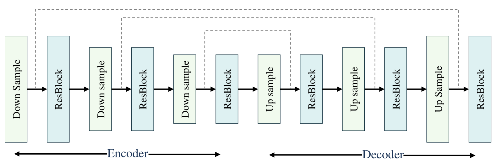
Figure 5: Block diagrams showing the deep encoder-decoder.

As depicted in Fig. 5, the Unet is a deep encoder-decoder structure, which is composed of one input layer, one encoder block, one decoder block, and one output layer. The hyperparameters and the details of each layer of Unet are introduced as follows.

V-A1 Input and Output Layers

To extract features from the complex-valued input data, we separate the input as the real part and the imaginary part as

$$\tilde{\boldsymbol{\psi}}_{\mathrm{u}}=\mathcal{M}(\mathrm{Re}\{\boldsymbol{\psi}_{\mathrm{u}}\},\mathrm{Im}\{\boldsymbol{\psi}_{\mathrm{u}}\}),$$ (41)

where $\mathcal{M}(\cdot)$ represents a mapping function. Similarly, the output of the network is given by

$$\hat{\mathbf{z}}_{\mathrm{u}}=\mathcal{M}^{-1}(D_{\mathrm{h}}(\tilde{\boldsymbol{\psi}}_{\mathrm{u}})),$$ (42)

where $\mathcal{M}^{-1}$ denotes a mapping function that constructs the complex-valued matrix from the real-valued components.

V-A2 Encoder and Decoder Layers

The encoder is composed of a series of downsample and upsample convolution blocks, which systematically reduce the spatial dimensions while increasing the number of feature channels. Each downsample convolution block incorporates $N_{c}$ sequential layers of $3\times 3\times 3$ convolution operations, which are subsequently processed by rectified linear unit (ReLU) activation and batch normalization (BN). As the network depth grows, the training process becomes increasingly susceptible to instability, making it challenging to achieve convergence to an optimal local minimum. To address this issue, we adopt a residual learning framework inspired by ResNet [27]. Specifically, the basic block of our network is designed as a residual block, which integrates $3\times 3\times 3$ convolution units alongside a projection shortcut implemented through a $1\times 1\times 1$ convolution. This projection shortcut preserves the flow of shallow-level information, ensuring gradient propagation and mitigating the vanishing gradient problem. By combining these shortcuts with skip connections, our architecture facilitates both local and global information interactions, significantly enhancing the network’s representational capacity.

Algorithm 1 UPnP for OTFS channel estimation

1:Transmitted pilot $\boldsymbol{\Phi}_{\mathrm{DD}}$, received signal $y_{\mathrm{DD}}$, number of iterations $N_{K}$

2:Estimated $\mathbf{h}^{N_{K}}$

3:Initialize auxiliary ${\mathbf{z}}_{\mathrm{h}}^{0}$, $\mathbf{u}_{\mathrm{h}}^{0}$ and ${\mathbf{h}}^{0}$

4:for $k=1,2,\dots,N_{K}$ do

5:  $\mathbf{h}^{k}=\mathrm{prox}_{f_{\mathrm{h}}}(\dot{\mathbf{z}}_{\mathrm{h}}^{k-1})$

6:  $\mathbf{z}_{\mathrm{h}}^{k}=D_{\mathrm{h}}(\dot{\mathbf{h}}^{k})$

7:  $\mathbf{u}_{\mathrm{h}}^{k}=\mathbf{u}_{\mathrm{h}}^{k-1}+(\mathbf{h}^{k}-\mathbf{z}_{\mathrm{h}}^{k})$

8:end for

V-B FC-based PnP for Symbol Detection

This subsection describes the proposed FPnP algorithm for the symbol detection problem. The overall symbol detection method is detailed in Algorithm 2. Let us first analyze the channel estimation error as

$$\mathbf{H}_{\mathrm{DD}}=\hat{\mathbf{H}}_{\mathrm{DD}}+\mathbf{E}_{\mathrm{DD}},$$ (43)

where $\hat{\mathbf{H}}_{\mathrm{DD}}$ and $\mathbf{E}_{\mathrm{DD}}$ are the estimated channel matrix and estimation error, respectively. Similar to [28], $\hat{\mathbf{H}}_{\mathrm{DD}}$ and $\mathbf{E}_{\mathrm{DD}}$ are unrelated, and the entries of $\mathbf{E}_{\mathrm{DD}}$ are zero mean CSCG with variance $\frac{1}{MN}\sigma_{e}^{2}$. The term $\frac{1}{MN}\sigma_{e}^{2}$ represents the error level of the channel estimation, and we assume it is unknown to the receiver. Therefore, the symbol detection model can be written as

$$\mathbf{y}_{\mathrm{DD}} =\hat{\mathbf{H}}_{\mathrm{DD}}\mathbf{x}_{\mathrm{DD}}+\mathbf{E}_{\mathrm{DD}}\mathbf{x}_{\mathrm{DD}}+\mathbf{n}_{\mathrm{DD}}$$

$$=\hat{\mathbf{H}}_{\mathrm{DD}}\mathbf{x}_{\mathrm{DD}}+\hat{\mathbf{n}}_{\mathrm{DD}},$$ (44)

where the entries of $\hat{\mathbf{n}}_{\mathrm{DD}}$ is CSCC noise with variance $\sigma^{2}_{\mathrm{d}}+\sigma^{2}_{e}$ when $MN$ is large enough. Accordingly, the OTFS symbol detection can be reformulated as

$$\min_{\mathbf{x}_{\mathrm{DD}}}\frac{1}{2}||\mathbf{y}_{\mathrm{DD}}-\hat{\mathbf{H}}_{\mathrm{DD}}\mathbf{x}_{\mathrm{DD}}||^{2}+\lambda_{\mathrm{x}}\mathcal{J}_{\mathrm{x}}(\mathbf{x}_{\mathrm{DD}}),$$ (45)

where $\lambda_{\mathrm{x}}$ and $\mathcal{J}_{\mathrm{x}}(\cdot)=\mathbf{x}_{\mathrm{DD}}\in\mathbb{Q}^{MN\times 1}$ denote the penalty parameter and symbol prior, respectively.

Following the PnP framework, the model-based step for updating $\mathbf{x}_{\mathrm{DD}}^{k}$ is given by

$$\mathbf{x}_{\mathrm{DD}}^{k+1} =\arg\min_{\mathbf{x}_{\mathrm{DD}}}\frac{1}{2}\left\|\mathbf{y}_{\mathrm{DD}}-\hat{\mathbf{H}}_{\mathrm{DD}}\mathbf{x}_{\mathrm{DD}}\right\|_{2}^{2}+\frac{\rho_{\mathrm{x}}}{2}\left\|\mathbf{x}_{\mathrm{DD}}-\mathbf{\dot{z}}_{\mathrm{x}}^{k})\right\|_{2}^{2}$$

$$=\mathbf{W}^{-1}(\hat{\mathbf{H}}_{\mathrm{DD}}^{H}\mathbf{y}_{\mathrm{DD}}+\rho_{\mathrm{x}}\,\mathbf{\dot{z}}_{\mathrm{x}}^{k}),$$ (46)

where $\mathbf{W}=(\hat{\mathbf{H}}_{\mathrm{DD}}^{H}\hat{\mathbf{H}}_{\mathrm{DD}}+\rho_{\mathrm{x}}\,\mathbf{I}_{\mathrm{MN}})$ and $\rho_{\mathrm{x}}$ denotes the penalty parameter. To reduce the computational complexity of symbol detection, we perform $\mathbf{W}^{-1}$ in the time domain. According to (23), the inverse matrix can be written as

$$\mathbf{W}^{-1} =\left(\mathbf{F}_{N}\otimes\mathbf{I}_{\mathrm{M}}\right)\left(\hat{\mathbf{H}}^{H}_{\mathrm{T}}\hat{\mathbf{H}}_{\mathrm{T}}+\rho_{\mathrm{x}}\mathbf{I}_{\mathrm{MN}}\right)^{-1}\left(\mathbf{F}_{N}^{\mathrm{H}}\otimes\mathbf{I}_{\mathrm{M}}\right),$$ (47)

where $\hat{\mathbf{H}}_{\mathrm{T}}$ denotes the estimated channel matrix in the time domain. Thanks to the block-diagonal structure of $\hat{\mathbf{H}}_{\mathrm{T}}$, we can perform the inverse matrix with low computational complexity with inverse submatrix, i.e., [29]

$$\left(\hat{\mathbf{H}}^{H}_{\mathrm{T}}\hat{\mathbf{H}}_{\mathrm{T}}+\rho_{\mathrm{x}}\mathbf{I}_{\mathrm{MN}}\right)^{-1}=\operatorname{diag}\{\mathbf{C}^{-1}_{1},\cdots,\mathbf{C}^{-1}_{N}\},$$ (48)

where $\mathbf{C}_{n}=\left({\hat{\mathbf{H}}_{n}^{H}\hat{\mathbf{H}}_{n}+\rho_{\mathrm{x}}\mathbf{I}_{\mathrm{M}}}\right)\in\mathbb{C}^{M\times M}$ are the diagonal sub-block of channel matrix $\mathbf{W}$.

Algorithm 2 FPnP for OTFS symbol detection

1:Estimated channel $\hat{\mathbf{H}}_{\mathrm{DD}}$, received signal $\mathbf{y}_{\mathrm{DD}}$, number of iterations $N_{K}$

2:Estimated symbol $\mathbf{x}_{\mathrm{DD}}^{N_{K}}$

3:Initialize auxiliary $\dot{\mathbf{z}}_{\mathrm{x}}^{0}$, $\mathbf{u}_{\mathrm{x}}^{0}$ and ${\mathbf{x}}_{\mathrm{DD}}^{0}$

4:for $k=1,2,\dots,N_{K}$ do

5:  $\mathbf{x}_{\mathrm{DD}}^{k}=\mathrm{prox}_{f_{\mathrm{x}}}(\dot{\mathbf{z}}_{\mathrm{x}}^{k-1})$

6:  $\mathbf{z}_{\mathrm{x}}^{k}=F_{\mathrm{x}}(\dot{\mathbf{x}}_{\mathrm{DD}}^{k})$

7:  $\mathbf{u}_{\mathrm{x}}^{k}=\mathbf{u}_{\mathrm{x}}^{k-1}+(\mathbf{x}_{\mathrm{DD}}^{k}-\mathbf{z}_{\mathrm{x}}^{k})$

8:end for

Since the decoupling operation is already performed in (46), the update for auxiliary variable $\mathbf{\dot{z}}_{\mathrm{x}}^{k}$ becomes a denoising task. For the learning-based denoiser, we employ a DL-based sequence detection method and soft information technology to obtain the auxiliary variable. Based on the type of constellation, we propose updating the auxiliary variables $\mathbf{z}_{\mathrm{u}}$ as

$$\mathbf{z}_{\mathrm{x}}^{k+1}=\arg\min_{\mathbf{z}_{\mathrm{x}}}\mathcal{J}_{\mathrm{x}}\left(\mathbf{z}_{\mathrm{x}}\right)+\frac{1}{2\sigma_{\mathrm{x}}^{2}}\left\|\mathbf{z}_{\mathrm{x}}-\mathbf{\dot{x}}_{\mathrm{DD}}^{k+1}\right\|_{2}^{2}=F_{\mathrm{x}}(\mathbf{\dot{x}}_{\mathrm{DD}}^{k+1}),$$ (49)

where $\sigma_{\mathrm{x}}=\frac{\lambda_{\mathrm{x}}}{2\rho_{\mathrm{x}}}$, and $F_{\mathrm{x}}(\cdot)$ represents the proposed FC-based update method. The pre-trained FN-based denoiser, denoted as $D_{\mathrm{x}}(\cdot)$, is depicted in Fig. 6. The $2MN$ input neurons are fed to the FC network, which consists of 3 hidden layers and one softmax activation layer. The input neurons, consisting of the real and imaginary parts of the input vector $\mathbf{\dot{x}}_{\mathrm{DD}}^{k+1}$, are processed by the FC network and then passed through the final softmax layer to produce $q^{\prime}=|\mathbb{Q}|$ outputs. The $q^{\prime}$ output neurons correspond to the size of the modulation alphabet, with each neuron representing the probability of a particular constellation point in the alphabet. To further improve the detection accuracy, we exploit the constellation prior and update $\mathbf{z}_{\mathrm{x}}^{k+1}$ via a soft mapper as

$$z^{k+1}[m^{\prime}]=\sum_{q\in\mathbb{Q}}p\{\dot{x}_{\mathrm{DD}}^{k+1}[m^{\prime}]|z_{\mathrm{x}}^{k+1}[m^{\prime}]=q\}\times q,$$ (50)

where $\dot{x}_{\mathrm{DD}}^{k+1}[m^{\prime}]$ with $m^{\prime}\in[1,MN]$ is the element of $\mathbf{\dot{x}}_{\mathrm{DD}}^{k+1}$. After completing FPnP-based detection for all $MN$ symbols, we use (46) to obtain $\mathbf{\dot{x}}_{\mathrm{DD}}^{k+2}$ at the $k+2$ iteration. In contrast to the completely data-based DL, we effectively utilize the estimated channel information and DL to achieve more accurate symbol detection results.

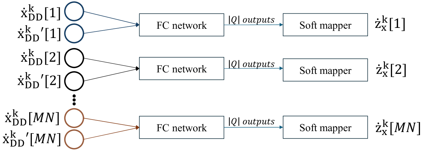
Figure 6: The proposed FC network for symbol detection, with 3 hidden layers and one softmax activation layer.

The complexity of the FPnP detector in one iteration is expressed as $O\left(M^{3}N+I_{L}\sum_{l}^{L}z_{l-1}z_{l})\right)$, where $I_{L}$ is the layer numbers of the FC network, $z_{l}$ is the neuron number at the $l$-th layer. In the offline training phase, we train an adaptive denoiser for the PnP framework with the complexity being $O\left(I_{t}I_{L}\sum_{l}^{L}z_{l-1}z_{l})\right)$, with $I_{t}$ indicating the number of training epochs. Compared to the conventional LS and LMMSE detectors, whose complexity is given by $\left(M^{3}N^{3}\right)$, the proposed detector exhibits significantly lower computational complexity.

Table I: Computational Complexities of Different Algorithms

Alrogithm	Offline Training	Online Estimation
LS	-	$O\left(M^{3}N^{3}\right)$
LMMSE	-	$O\left(M^{3}N^{3}\right)$
FPnP	$O\left(I_{t}I_{L}\sum_{l}^{L}z_{l-1}z_{l})\right)$	$O\left(M^{3}N+I_{L}\sum_{l}^{L}z_{l-1}z_{l})\right)$

VI Simulation Results

This section evaluates the effectiveness of the proposed method via simulation results. The parameter configurations are first described, followed by the presentation of results for channel estimation and symbol detection, respectively. The convergence of the PnP framework-based methods is then demonstrated.

VI-A Parameters Setting

An OTFS frame is configured with $N=20$ and $M=20$, corresponding to 20 time slots and 20 subcarriers in the TF domain. The system operates at a carrier frequency of $f_{c}=3$ GHz with a subcarrier spacing of 7.5 kHz. The maximum delay index and Doppler index are set as $k_{\max}=3$ and $l_{\max}=4$, respectively. The number of channel paths is $P=4$, and the associated delay and Doppler indices for each channel path are randomly selected from $[0,l_{\max}]$ and $[-k_{\max},k_{\max}]$, respectively. The channel gain follows the distribution $\mathcal{CN}(0,\frac{1}{P})$. The signal-to-noise ratio (SNR) for the transmission is defined as $\mathrm{SNR}=\frac{E_{s}}{N_{0}}$, where symbol energy $E_{s}$ is normalized to 1. Moreover, we generate the dataset using the Monte-Carlo method. The training set and validation set consist of $90,000$ and $10,000$ samples, respectively, which are employed to train the DL-based denoisers. The added random Gaussian noise is uniformly generated in the range of $[0,50]$ dB. For online estimation, each presented result is obtained by averaging over $2,000$ Monte-Carlo realizations. We execute the proposed method on a desktop computer equipped with a Xeon Gold 6226R 2.9 GHz processing unit (CPU) and an NVIDIA GeForce RTX 3090 graphics processing unit (GPU). Note that the Adam optimizer is adopted for network training, with the learning rate set to 0.001. For the PnP-based channel estimation and symbol detection methods, the regularization parameters $\lambda_{\mathrm{x}}=\lambda_{\mathrm{h}}$ and the penalty factors $\rho_{\mathrm{x}}=\rho_{\mathrm{h}}$ are tuned and set to $0.5$ and $0.1$, respectively.

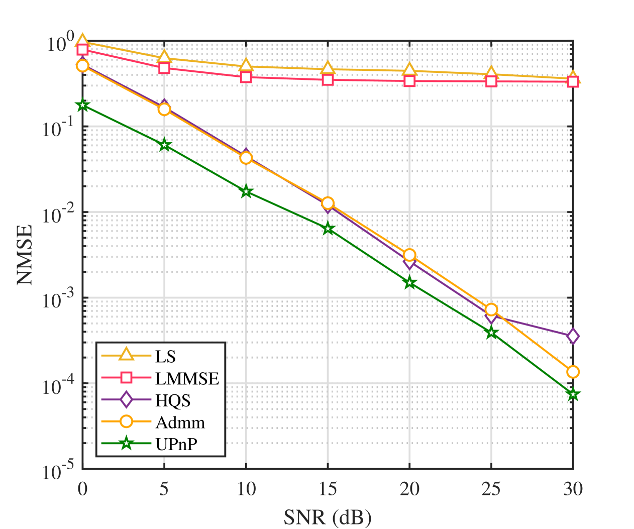
Figure 7: The performance comparison for channel estimation.

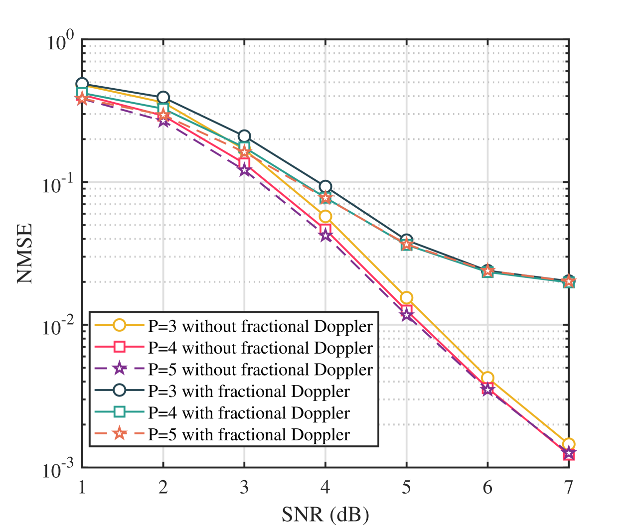
Figure 8: Robust performance comparison under different channel conditions

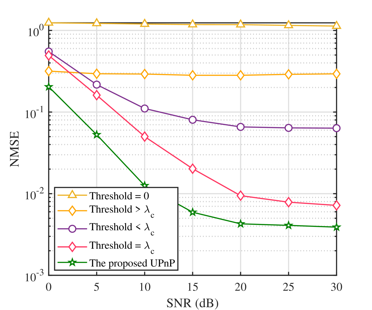
Figure 9: Performance comparison of the proposed UPnP and traditional algorithms with deterministic psriors

VI-B Results for Channel Estimation

We provide simulations of the following algorithms for comparison: the LS method, the LMMSE method, the HQS method [25], and the ADMM method [30]. The channel estimation performance, evaluated in terms of NMSE across various SNR levels, is illustrated in Fig. 7. A noticeable performance gap is observed between the LS and LMMSE methods, as the LMMSE can capture the prior information of the noise, while the LS method does not leverage any knowledge about the channel or noise statistics. The HQS achieves better NMSE than both LS and LMMSE by iteratively solving the optimization problem associated with channel estimation, however, its performance is constrained by the approximation introduced in quadratic splitting. The ADMM demonstrates similar performance compared to HQS across most SNR levels, which can be attributed to its better convergence properties and robustness to noise. Compared with benchmarks, our proposed UPnP outperforms all other methods across the entire SNR range. The data-driven capability of the denoiser enables the UPnP to capture channel characteristics more effectively. Furthermore, the integration of PnP techniques allows the algorithm to balance model-driven and data-driven components, achieving remarkable NMSE reductions, especially at higher SNR levels.

In addition, we demonstrate the robustness of the algorithm under different OTFS channel conditions, as shown in Fig. 8. It can be observed that the proposed method performs significantly better in the absence of fractional Doppler. This improvement can be attributed to the higher sparsity of the channel with integer delay and Doppler, which allows the UPnP to effectively capture the features of the input. In contrast, when fractional Doppler is present, the channel sparsity decreases, leading to a corresponding degradation in performance. Additionally, it can be observed that small variations in the path number $P$ do not significantly affect the algorithm’s performance.

Furthermore, we present a performance comparison between the proposed method and traditional algorithms with deterministic priors. As shown in Fig. 9, the NMSE performance of the traditional algorithm is the worst when the threshold equals 0, as no prior constraints are applied. Here, the threshold is used for the soft-thresholding operator in traditional algorithms. When the threshold is too large, resulting in the excessive removal of valid terms, or too small, causing the retention of excessive noise, the performance is further degraded. Traditional methods require threshold adjustment, which can significantly impact the algorithm’s performance. When the threshold is set to $\lambda_{c}=\lambda_{\mathrm{h}}/\rho_{\mathrm{h}}$, the estimation accuracy improves due to the effectiveness of the $\ell_{1}$-norm in accurately capturing the sparsity of the OTFS channel. Nevertheless, the proposed method outperforms conventional approaches. This superiority can be attributed to the UPnP method, which utilizes a trained denoiser to capture intricate channel characteristics, thereby enabling more precise channel estimation.

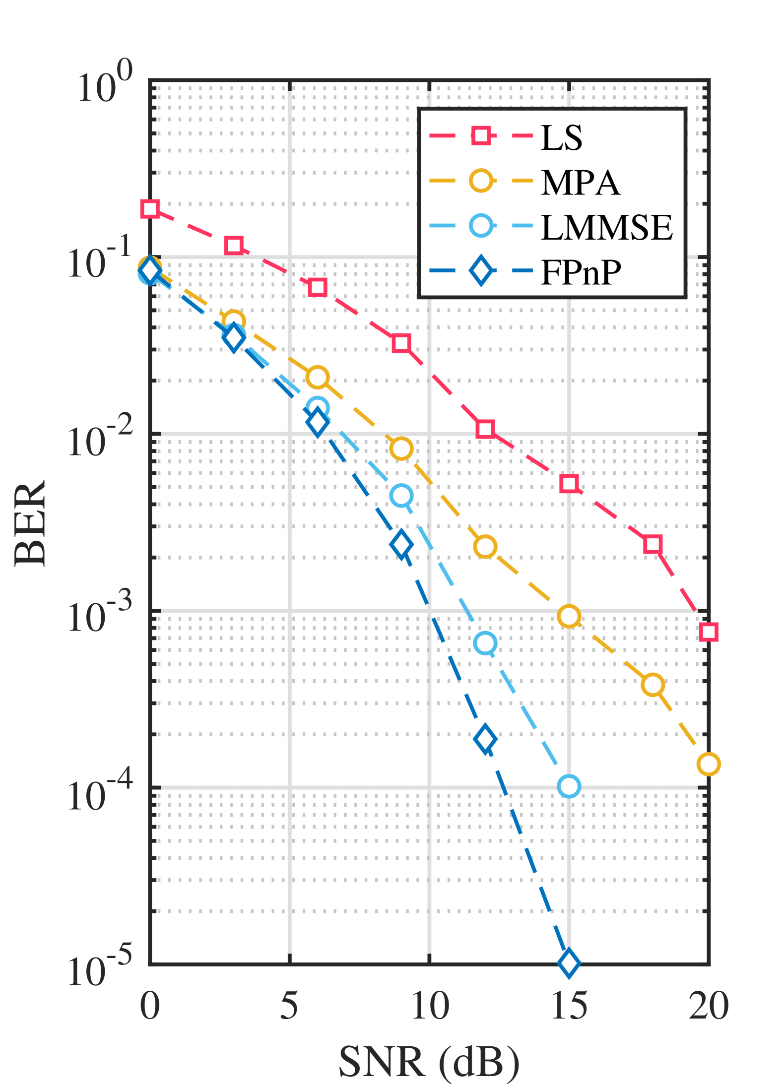
(a) Integer Doppler.

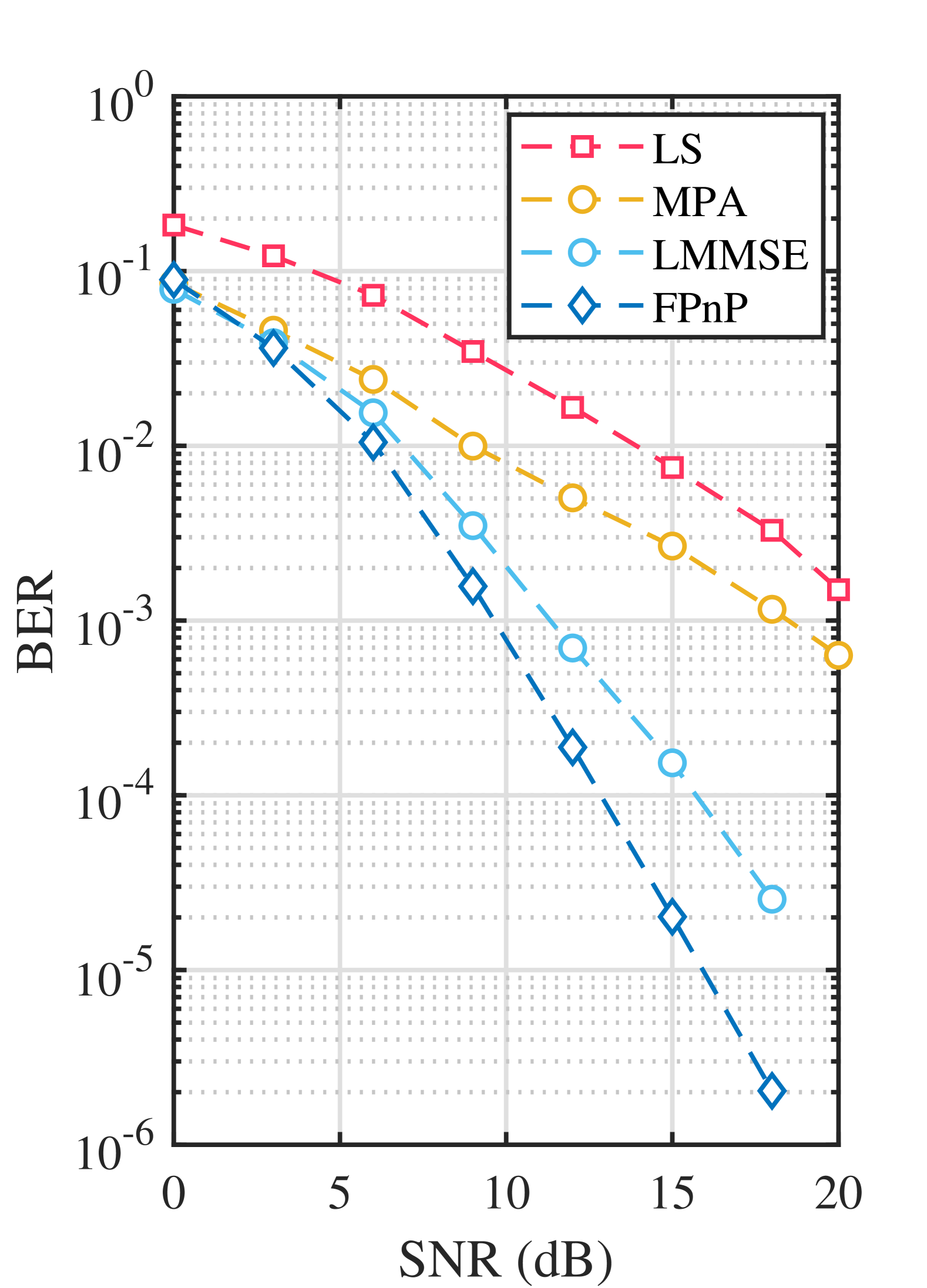
(b) Fractional Doppler.

Figure 10: BER performance comparison with baselines for symbol detection.

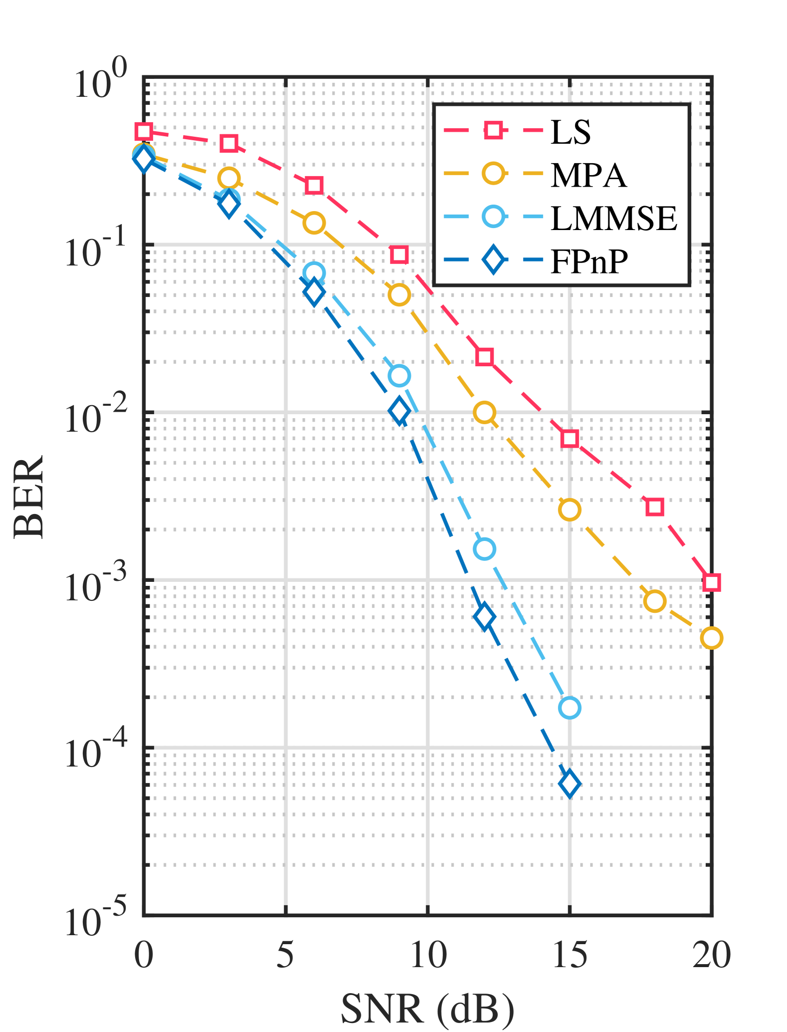
(a) BER comparison with slightly imperfect CSI.

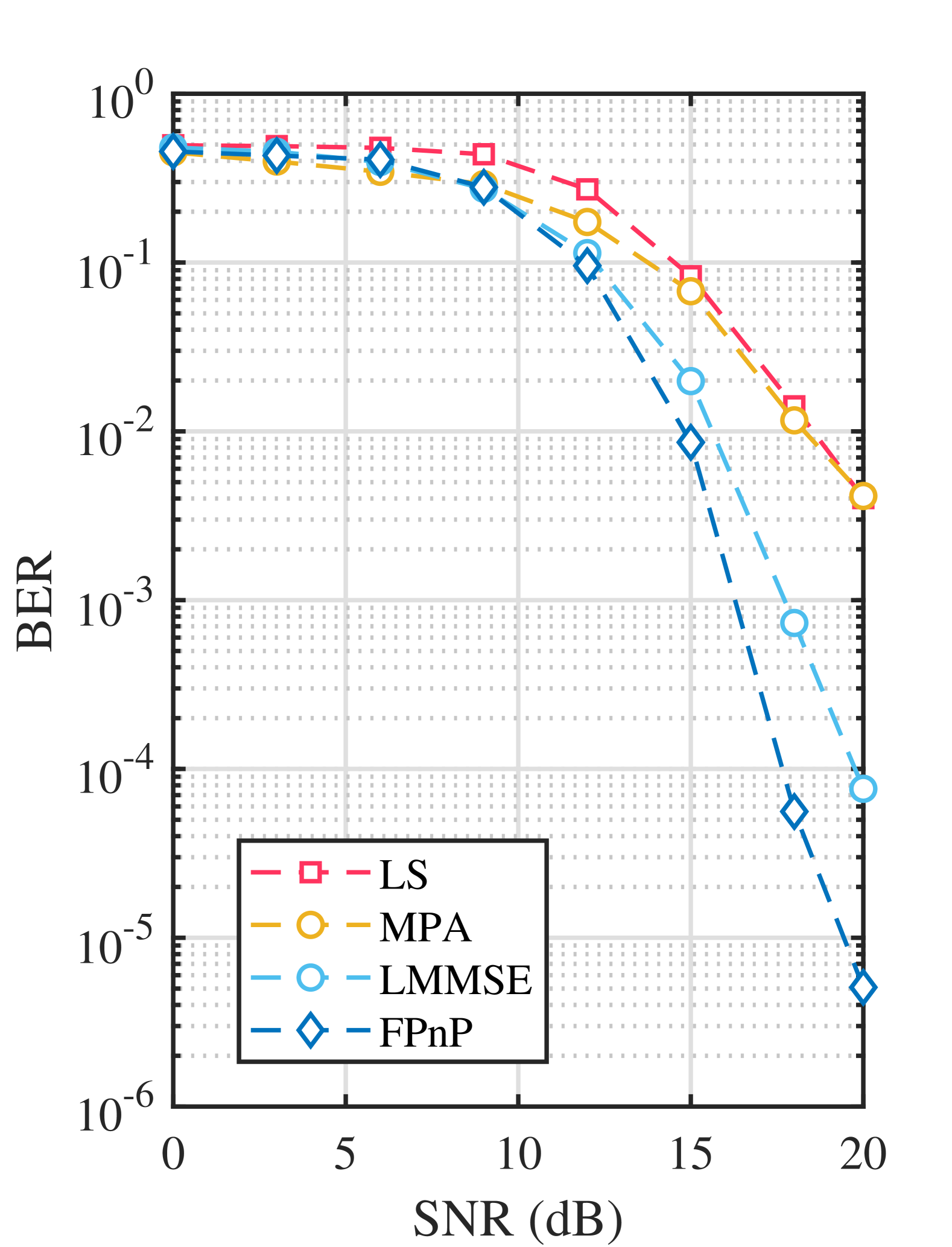
(b) BER comparison with severely imperfect CSI.

Figure 11: BER comparison with non-ideal channel.

VI-C Results for Symbol Detection

In this section, we first investigate the reliability of the FPnP-based symbol detection algorithm. In particular, we evaluate the BER performance under different received SNRs with various symbol detection algorithms. Fig. 10(a) presents the curves of BER versus SNR with the integer delay and Doppler in the OTFS effective channel. It can be observed that the LS method has the worst performance since no prior noise statistics have been utilized in the detection. We can also find that the MPA outperforms the LS estimator. This is because the MPA can effectively incorporate prior knowledge, such as sparsity or the statistical properties of the channel. The LMMSE algorithm achieves better performance as it treats the transmitted symbol prior as a Gaussian distribution. In contrast, the proposed FPnP algorithm exhibits the best performance as the FPnP employs a trained denoiser to adaptively mitigate noise interference. As shown in Fig. 10(b), the performance of all algorithms degrades in the presence of fractional Doppler. It can be observed that the MPA algorithm is the most significantly affected by the presence of fractional Doppler shifts. This is because the MPA algorithm is dependent on the sparsity or structural characteristics of the channel. When fractional Doppler effects are introduced, the channel’s sparsity no longer aligns with the assumptions inherent to the MPA algorithm, leading to a degradation in its performance. In contrast, other algorithms exhibit greater robustness under fractional Doppler shifts, maintaining consistent performance despite the lack of alignment with the sparsity assumptions.

Furthermore, we investigate the impact of the channel estimation error on the BER performance of different algorithms, as shown in Fig. 11(a). Among the evaluated algorithms, the FPnP algorithm consistently presents superior performance, achieving the lowest BER across the full SNR range. These results are expected since our proposed method with the embedded neural network can learn the features of the symbols and interference to guarantee the BER performance. Fig. 11(b) illustrates BER performance for four baselines when the severely imperfect CSI is used. It can be observed that all four algorithms exhibit similar BER performance at low SNR regions, which indicates that the noise dominates the system and limits the impact of the algorithm’s inherent robustness to channel estimation errors. As the SNR increases, the LS and MPA algorithms consistently exhibit the worst BER performance, particularly at higher SNRs. While the LMMSE algorithm outperforms MPA across all SNRs, it experiences noticeable performance degradation compared to the FPnP algorithm as SNR increases. This increasing gap indicates that the LMMSE algorithm is more sensitive to larger channel errors. Meanwhile, our proposed FPnP algorithm demonstrates significant robustness under realistic and imperfect channel conditions.

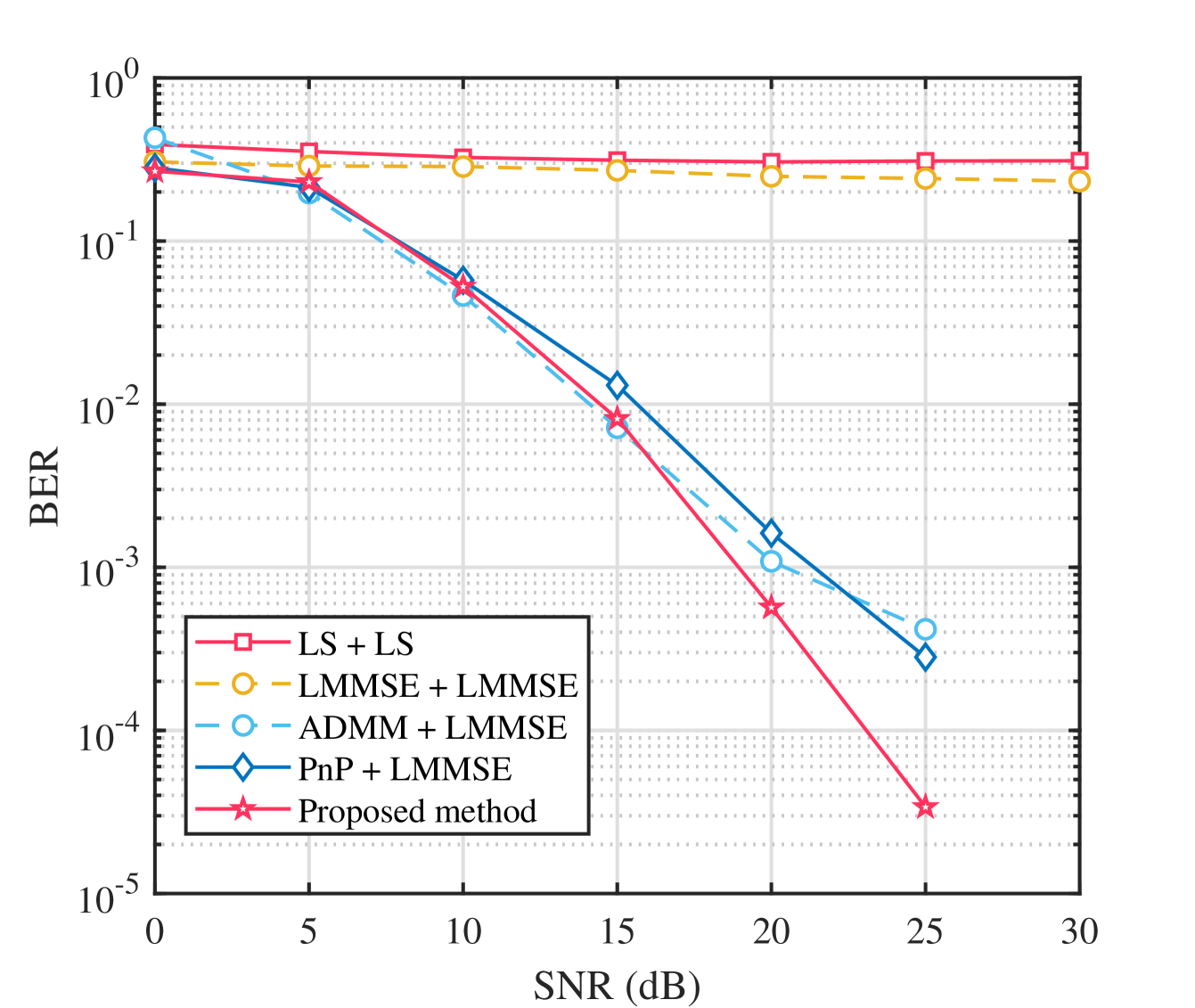
Figure 12: BER performance for sequential channel estimation and symbol detection.

We investigate the BER performance of sequential channel estimation and symbol detection, where channel estimation is performed first, and the estimated CSI is then used for symbol detection. As illustrated in Fig. 12, we evaluate our proposed method against four baselines: (1) LS + LS, (2) LMMSE + LMMSE, (3) ADMM + LMMSE, (4) UPnP + LMMSE, and (5) our proposed method (UPnP + FPnP). It can be observed that the conventional LS + LS and LMMSE + LMMSE approaches demonstrate the poorest performance, particularly in low SNR conditions. This performance degradation stems from their limited channel estimation accuracy, which directly impacts symbol detection reliability. In contrast, the ADMM + LMMSE method shows notable improvement, especially in low-SNR scenarios. The iterative optimization process of ADMM enables more robust channel estimation compared to traditional LS and LMMSE methods, effectively reducing BER at lower SNR values. The UPnP + LMMSE estimator demonstrates superior performance over both LS and standard LMMSE methods, benefiting from enhanced channel estimation accuracy through the proposed DL-based estimation method. This improvement leads to more reliable symbol detection and significantly lower BER, particularly in high-SNR conditions. It can be demonstrated that the proposed method achieves the best BER curve, primarily due to the integration of UPnP and FPnP data-driven capabilities, which enable accurate channel estimation and robust symbol detection even in the presence of channel estimation errors.

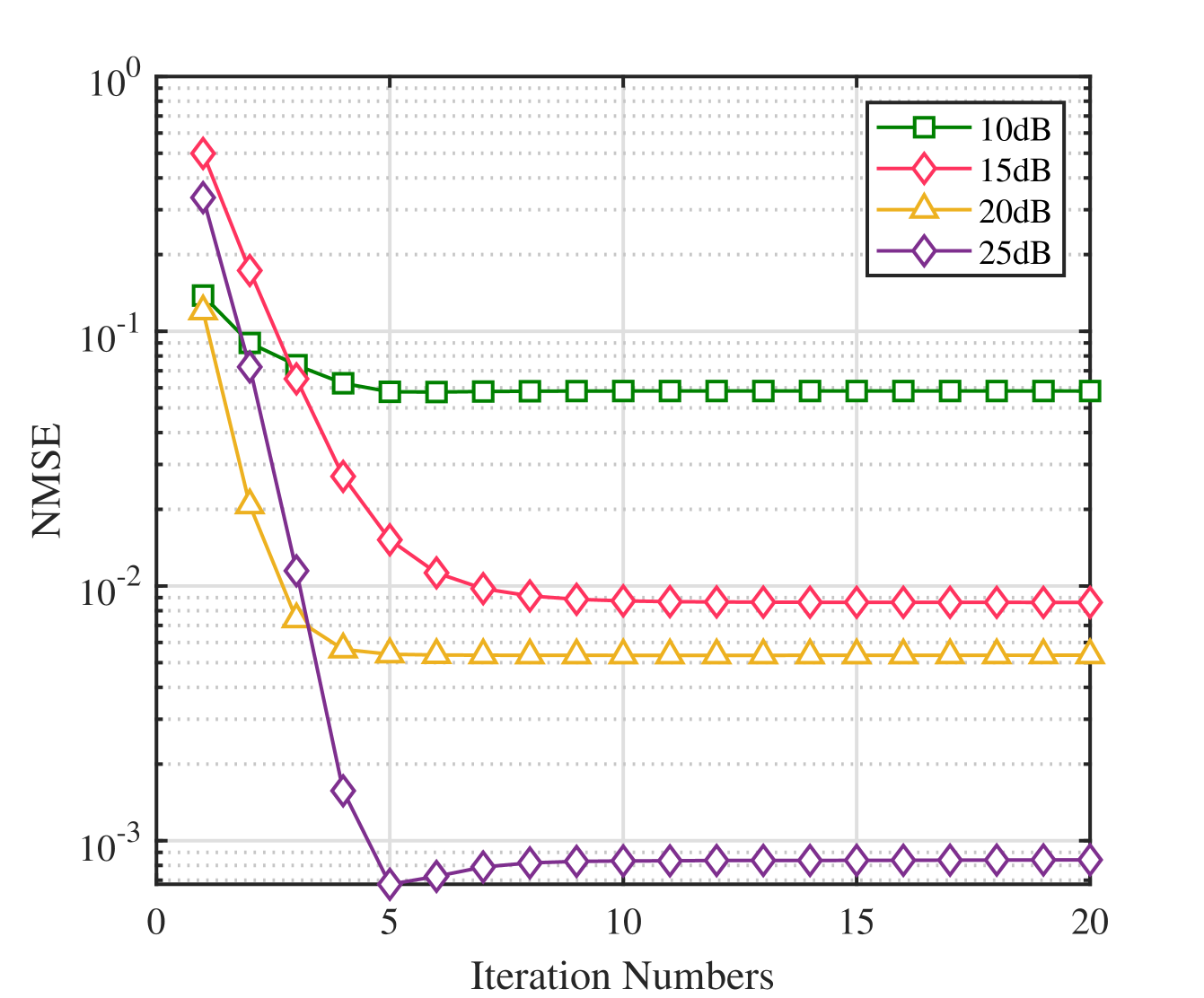
Figure 13: The convergence of UPnP-based method for channel estimation.

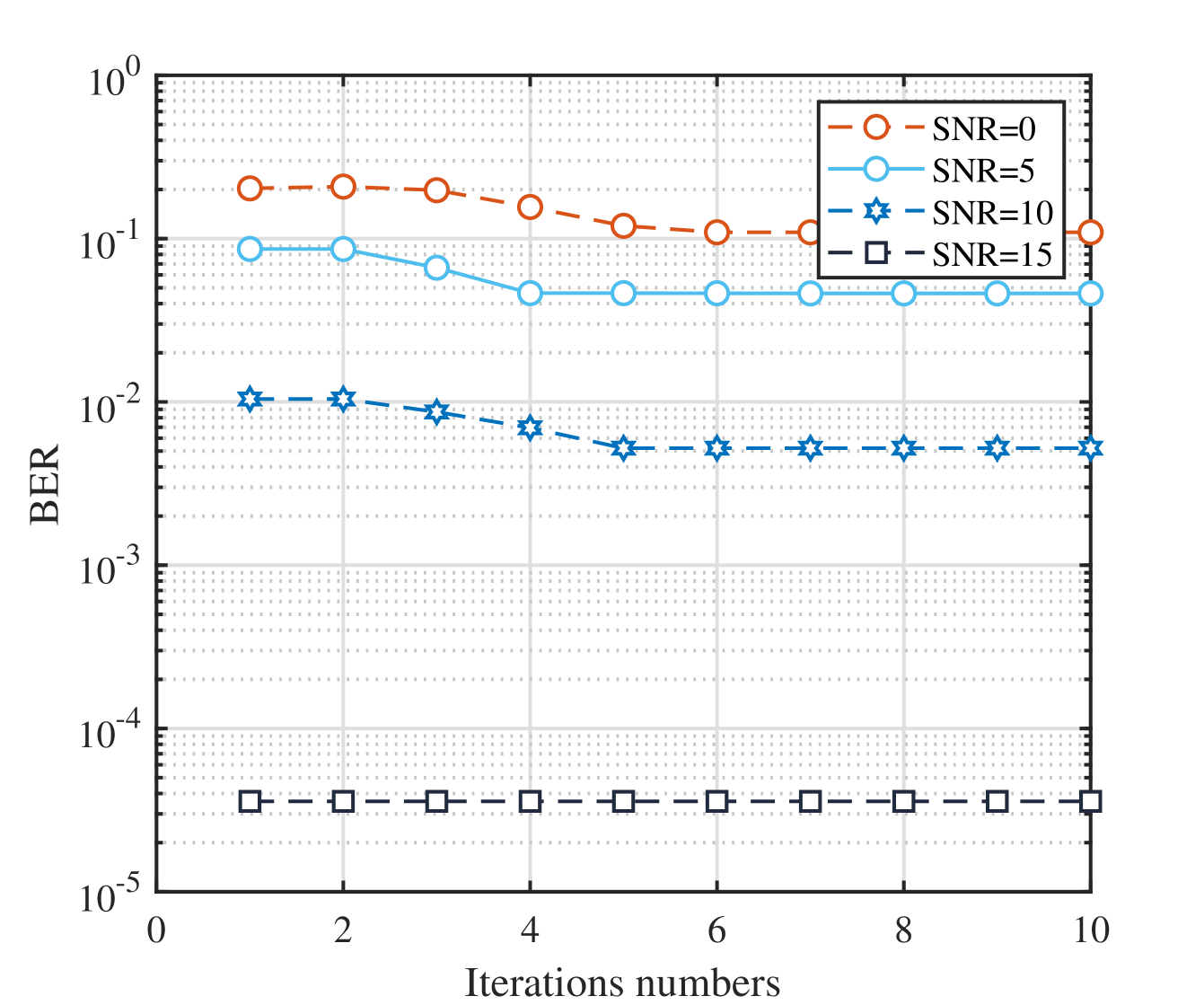
Figure 14: The convergence of the FPnP-based method for symbol detection.

VI-D Convergence

Recent theoretical studies have extensively investigated the convergence properties of deep PnP prior algorithms. In [31], the authors established sufficient conditions for the convergence of such algorithms, emphasizing that the denoising operator must function as a proximal mapping. Subsequent research has expanded these findings by providing convergence guarantees under more specific conditions, such as bounded and continuous denoisers [32]. Furthermore, extensive empirical evidence has demonstrated the practical effectiveness of DL-based denoisers within the PnP framework [33]. In the following, we empirically evaluate the convergence of the PnP framework using the UPnP and FPnP algorithms for OTFS channel estimation and symbol detection. Fig. 13 demonstrates the convergence of the proposed UPnP-based channel estimation approach. The NMSE decreases rapidly during the initial iterations, typically within the first five iterations, indicating the efficiency of the proposed algorithm in achieving significant error reduction early in the iterative process. Furthermore, Fig. 14 illustrates the BER convergence curves under different SNRs. It can be observed that for smaller SNRs, BER exhibits a rapid decline during the initial iterations and then stabilizes subsequently. Therefore, the proposed algorithm converges rapidly within a few iterations. It is important to note that the proposed deep PnP prior framework implicitly utilizes a DL-based denoising operator as the regularizer. The empirical convergence patterns observed in the results suggest that DL-based denoisers may introduce implicit regularization effects that contribute to the stabilization of the iterative process.

VII Conclusions

In this paper, we explored DL-based channel estimation and symbol detection for OTFS. To achieve this, we developed a unified deep learning-based PnP framework. Specifically, we decomposed the optimization objective into two separate subproblems: a prior-related term and a data-fidelity term. The prior-related subproblem was formulated as a denoising task, which can be effectively addressed through deep learning approaches. Subsequently, we integrated a pre-trained lightweight Unet architecture into the framework to develop the UPnP-based channel estimation method. For symbol detection, a trained FC-based denoiser was inserted into the framework to complete symbol detection. In addition, we simplified the model-based step by exploiting the measurement matrix in the time domain, thereby enhancing robustness and reducing complexity. This proposed hybrid approach maintains the flexibility of traditional optimization-based methods while capitalizing on the powerful data-driven capabilities of deep learning architectures. It enhances both channel estimation and symbol detection, demonstrating the potential of deep learning in improving OTFS performance in challenging wireless environments.

References

- [1] W. Yuan, Z. Wei, J. Yuan, and D. W. K. Ng, “A simple variational bayes detector for orthogonal time frequency space (OTFS) modulation,” IEEE Trans. Veh. Technol., vol. 69, no. 7, pp. 7976–7980, Jul. 2020.
- [2] Z. Ni, J. A. Zhang, X. Huang, K. Yang, and J. Yuan, “Uplink sensing in perceptive mobile networks with asynchronous transceivers,” IEEE Trans. Signal Process., vol. 69, pp. 1287–1300, 2021.
- [3] Z. Wei, W. Yuan, S. Li, J. Yuan, G. Bharatula, R. Hadani, and L. Hanzo, “Orthogonal time-frequency space modulation: A promising next-generation waveform,” IEEE Wireless Commun., vol. 28, no. 4, pp. 136–144, 2021.
- [4] M. Nie, S. Li, D. Mishra, J. Yuan, and D. W. K. Ng, “Uplink multi-user otfs: Transmitter design based on statistical channel information,” IEEE Trans. Commun., 2024.
- [5] X. Wang, W. Shen, C. Xing, J. An, and L. Hanzo, “Joint bayesian channel estimation and data detection for OTFS systems in LEO satellite communications,” IEEE Trans. Commun., vol. 70, no. 7, pp. 4386–4399, 2022.
- [6] P. Raviteja, K. T. Phan, and Y. Hong, “Embedded pilot-aided channel estimation for OTFS in delay–doppler channels,” IEEE Trans. Veh. Technol., vol. 68, no. 5, pp. 4906–4917, May. 2019.
- [7] W. Yuan, S. Li, Z. Wei, J. Yuan, and D. W. K. Ng, “Data-aided channel estimation for OTFS systems with a superimposed pilot and data transmission scheme,” IEEE Wireless Commun. Lett., vol. 10, no. 9, pp. 1954–1958, Sept. 2021.
- [8] X. Li and W. Yuan, “OTFS detection based on gaussian mixture distribution: A generalized message passing approach,” IEEE Commun. Lett., vol. 28, no. 1, pp. 178–182, 2023.
- [9] Z. Li, W. Yuan, and L. Zhou, “Uamp-based channel estimation for OTFS in the presence of the fractional doppler with HMM prior,” in 2022 IEEE/CIC Int. Conf. Commun. China (ICCC Workshops), 2022, pp. 304–308.
- [10] Z. Wei, W. Yuan, S. Li, J. Yuan, and D. W. K. Ng, “Transmitter and receiver window designs for orthogonal time-frequency space modulation,” IEEE Trans. Commun., vol. 69, no. 4, pp. 2207–2223, 2021.
- [11] H. Ye, G. Y. Li, and B.-H. Juang, “Power of deep learning for channel estimation and signal detection in OFDM systems,” IEEE Wireless Commun. Lett., vol. 7, no. 1, pp. 114–117, 2017.
- [12] L. Dai, R. Jiao, F. Adachi, H. V. Poor, and L. Hanzo, “Deep learning for wireless communications: An emerging interdisciplinary paradigm,” IEEE Wireless Commun., vol. 27, no. 4, pp. 133–139, 2020.
- [13] C. Liu, X. Liu, D. W. K. Ng, and J. Yuan, “Deep residual learning for channel estimation in intelligent reflecting surface-assisted multi-user communications,” IEEE Trans. Wireless Commun., vol. 21, no. 2, pp. 898–912, 2022.
- [14] X. Zhang, C. Liu, W. Yuan, J. A. Zhang, and D. W. K. Ng, “Sparse prior-guided deep learning for OTFS channel estimation,” IEEE Trans. Veh. Technol., pp. 1–6, 2024.
- [15] Y. Gong, Q. Li, F. Meng, X. Li, and Z. Xu, “Viterbinet-based signal detection for OTFS system,” IEEE Commun. Lett., vol. 27, no. 3, pp. 881–885, 2023.
- [16] K. Zhang, Y. Li, W. Zuo, L. Zhang, L. Van Gool, and R. Timofte, “Plug-and-play image restoration with deep denoiser prior,” IEEE Trans. Pattern Anal. Mach. Intell., vol. 44, no. 10, pp. 6360–6376, 2021.
- [17] Z. Lai, K. Wei, and Y. Fu, “Deep plug-and-play prior for hyperspectral image restoration,” Neurocomputing, vol. 481, pp. 281–293, 2022.
- [18] C. Liu, S. Li, W. Yuan, X. Liu, and D. W. K. Ng, “Predictive precoder design for OTFS-enabled URLLC: A deep learning approach,” IEEE J. Sel. Areas Commun., vol. 41, no. 7, pp. 2245–2260, 2023.
- [19] J. A. Zhang, H. Zhang, K. Wu, X. Huang, J. Yuan, and Y. J. Guo, “Wireless communications in doubly selective channels with domain adaptivity,” Accepted for IEEE Communications Magazine, 2024.
- [20] F. Liu, Z. Yuan, Q. Guo, Z. Wang, and P. Sun, “Message passing-based structured sparse signal recovery for estimation of OTFS channels with fractional doppler shifts,” IEEE Trans. Wireless Commun., vol. 20, no. 12, pp. 7773–7785, 2021.
- [21] P. Raviteja, Y. Hong, E. Viterbo, and E. Biglieri, “Practical pulse-shaping waveforms for reduced-cyclic-prefix OTFS,” IEEE Trans. Vehi. Tech., vol. 68, no. 1, pp. 957–961, 2019.
- [22] B. Shen, Y. Wu, J. An, C. Xing, L. Zhao, and W. Zhang, “Random access with massive mimo-otfs in LEO satellite communications,” IEEE J. Sel. Areas Commun., vol. 40, no. 10, pp. 2865–2881, 2022.
- [23] Z. Li, W. Yuan, and L. Zhou, “Uamp-based channel estimation for OTFS in the presence of the fractional doppler with hmm prior,” in 2022 IEEE/CIC Int. Conf. Commun. China (ICCC Workshops). IEEE, 2022, pp. 304–308.
- [24] E. Ryu, J. Liu, S. Wang, X. Chen, Z. Wang, and W. Yin, “Plug-and-play methods provably converge with properly trained denoisers,” in Int. Conf. Mach. Learning. PMLR, 2019, pp. 5546–5557.
- [25] W. Wan, W. Chen, S. Wang, G. Y. Li, and B. Ai, “Deep plug-and-play prior for multitask channel reconstruction in massive MIMO systems,” IEEE Trans. Commun., vol. 72, no. 7, pp. 4149–4162, 2024.
- [26] Y. LeCun, Y. Bengio, and G. Hinton, “Deep learning,” nature, vol. 521, no. 7553, pp. 436–444, 2015.
- [27] K. He, X. Zhang, S. Ren, and J. Sun, “Deep residual learning for image recognition,” in Proceedings of the IEEE Conf. Comput. Vis. Pattern Recog., 2016, pp. 770–778.
- [28] T. Yoo and A. Goldsmith, “Capacity of fading MIMO channels with channel estimation error,” in 2004 IEEE Int. Conf. Commun. (IEEE Cat. No. 04CH37577), vol. 2. IEEE, 2004, pp. 808–813.
- [29] H. Wen, W. Yuan, N. Wu, and J. Wen, “A low-complexity cross-domain OAMP detector for OTFS,” in 2022 Int. Sympos. Wireless Commun. Syst. (ISWCS), 2022, pp. 1–6.
- [30] W. Yuan, N. Wu, Q. Guo, Y. Li, C. Xing, and J. Kuang, “Iterative receivers for downlink MIMO-SCMA: Message passing and distributed cooperative detection,” IEEE Trans. Wireless Commun., vol. 17, no. 5, pp. 3444–3458, 2018.
- [31] S. Sreehari, S. V. Venkatakrishnan, B. Wohlberg, G. T. Buzzard, L. F. Drummy, J. P. Simmons, and C. A. Bouman, “Plug-and-play priors for bright field electron tomography and sparse interpolation,” IEEE Trans. Comput. Imag., vol. 2, no. 4, pp. 408–423, 2016.
- [32] S. Mukherjee, A. Hauptmann, O. Öktem, M. Pereyra, and C.-B. Schönlieb, “Learned reconstruction methods with convergence guarantees: A survey of concepts and applications,” IEEE Signal Process. Mag., vol. 40, no. 1, pp. 164–182, 2023.
- [33] M. Zhao, X. Wang, J. Chen, and W. Chen, “A plug-and-play priors framework for hyperspectral unmixing,” IEEE Trans. Geosci. Remote Sens., vol. 60, pp. 1–13, 2021.