GP-enhanced Autonomous Drifting Framework using ADMM-based iLQR
Abstract
Autonomous drifting is a complex challenge due to the highly nonlinear dynamics and the need for precise real-time control, especially in uncertain environments. To address these limitations, this paper presents a hierarchical control framework for autonomous vehicles drifting along general paths, primarily focusing on addressing model inaccuracies and mitigating computational challenges in real-time control. The framework integrates Gaussian Process (GP) regression with an Alternating Direction Method of Multipliers (ADMM)-based iterative Linear Quadratic Regulator (iLQR). GP regression effectively compensates for model residuals, improving accuracy in dynamic conditions. ADMM-based iLQR not only combines the rapid trajectory optimization of iLQR but also utilizes ADMM’s strength in decomposing the problem into simpler sub-problems. Simulation results demonstrate the effectiveness of the proposed framework, with significant improvements in both drift trajectory tracking and computational efficiency. Our approach resulted in a 38 reduction in RMSE lateral error and achieved an average computation time that is 75 lower than that of the Interior Point OPTimizer (IPOPT).
I INTRODUCTION
Autonomous driving technologies have made significant strides in recent years, yet performing high-dynamic maneuvers such as drifting remains a complex challenge. Drifting, characterized by the intentional over-steering of a vehicle to induce loss of rear-wheel traction while maintaining control through the front wheels, has garnered sustained attention in both academic and industrial research due to its unique dynamics and control challenges [1] [2]. This maneuver, while being an essential aspect of advanced driving, also presents considerable difficulties in terms of vehicle control, particularly when considering the highly nonlinear tire-road interactions and fast-changing dynamics involved.
Most existing drift control methods rely heavily on accurate dynamic models to stabilize the vehicle during these high-speed maneuvers. Traditional approaches, such as those in [3] and [4], explore error dynamic models and nonlinear model inversion to achieve the desired state trajectories for effective drift control. Similarly, optimization-based techniques like Model Predictive Control (MPC) have been widely adopted to manage the vehicle’s dynamic states around drift equilibrium points [5] [6] [7] [8]. However, while these methods have proven effective under well-modeled conditions, they remain highly dependent on the accuracy of the underlying vehicle dynamics model. Even small deviations in model parameters, such as a change in road friction, can result in significant performance degradation [9]. This reliance on precise models makes traditional methods vulnerable in uncertain or rapidly changing environments.
To address these limitations, machine learning techniques have been integrated, offering adaptability to unmodeled dynamics and improved model accuracy [10] [11]. Among machine learning techniques, Gaussian Processes (GP) have shown particular promise. Studies such as [12] [13] and [14] demonstrated GP’s effectiveness in capturing dynamic uncertainties and improving control performance.
However, the integration of GP into real-time control frameworks introduces significant computational challenges due to its nonparametric nature [13]. This creates a trade-off between model accuracy and computational efficiency, which becomes particularly problematic when combined with Nonlinear Model Predictive Control (NMPC), where real-time performance is essential.
To manage these computational demands and ensure effective constraint handling, the combination of the iterative Linear Quadratic Regulator (iLQR) [15] and the Alternating Direction Method of Multipliers (ADMM) [16] has emerged as a promising solution. iLQR is known for its efficiency in optimizing control trajectories for nonlinear systems, and recent studies have extended its application to handle more complex, constrained optimization tasks [17] [18] [19]. To further enhance iLQR’s ability to manage physical constraints, ADMM is employed as a complementary method. ADMM restructures the constrained optimization problem into smaller sub-problems, solving them sequentially while respecting the system’s physical limitations. ADMM has demonstrated success in various optimal control applications [20] [21] [22], making it a natural fit alongside iLQR without sacrificing real-time performance.
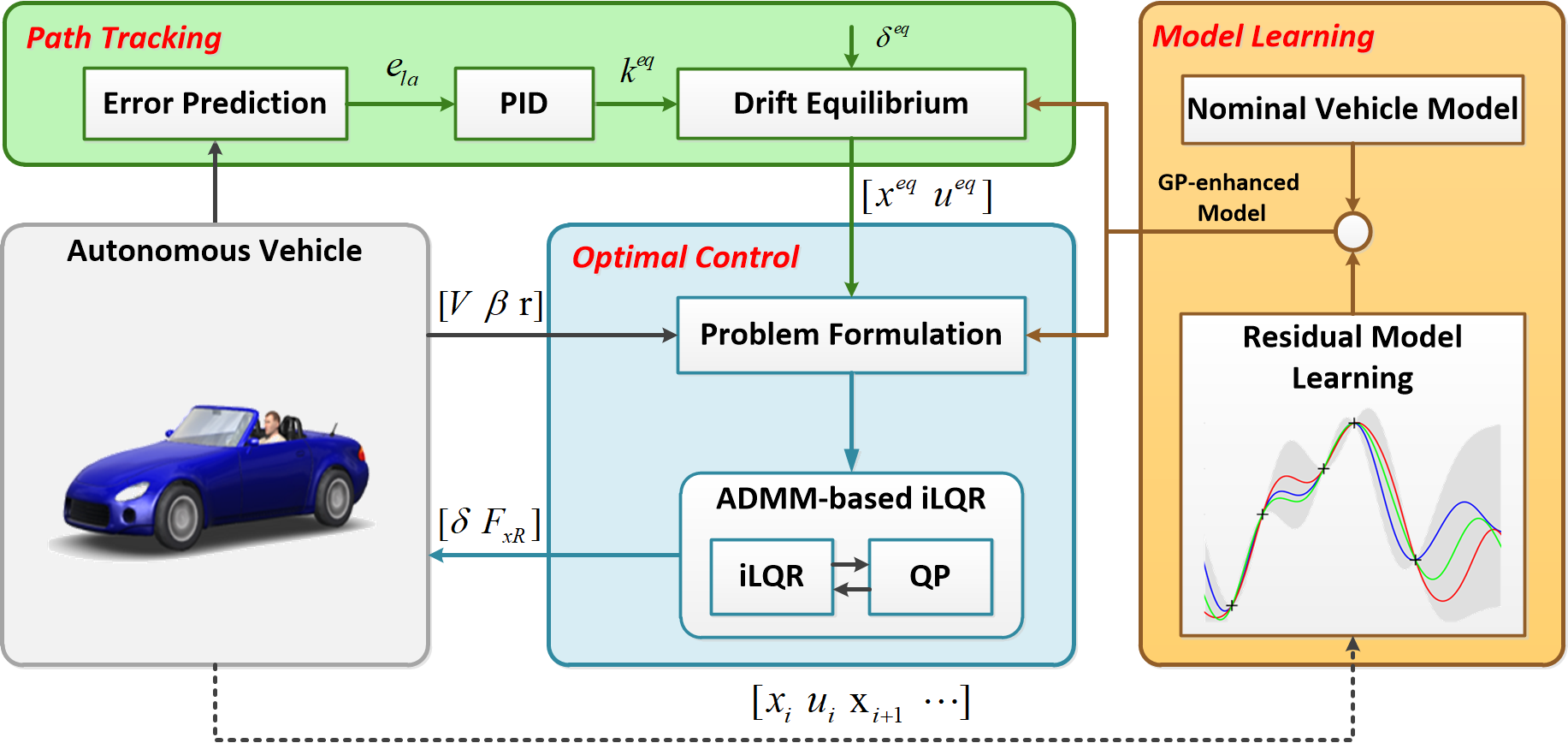
This paper presents a novel hierarchical control framework (Fig.1) for autonomous drifting along general paths, enhancing a relatively simple nominal model using GP and solving the highly nonlinear constrained optimal control problem efficiently through an ADMM-based iLQR. The main contributions of our work are as follows:
-
I.
A hierarchical control framework is proposed for autonomous drifting, enabling vehicles to follow general paths. GPs are employed to correct model mismatches, significantly enhancing performance.
-
II.
ADMM decomposes the optimization into two sub-problems, solved efficiently with iLQR and Quadratic Programming (QP), reducing computational burden.
-
III.
Simulation results highlight the framework’s effectiveness, showing a 38 reduction in lateral error with the integration of GP and a 75 decrease in average computation time compared to IPOPT. Additionally, the method demonstrates robustness under varying friction conditions.
II PRELIMINARIES
II-A Gaussian Process Regression
GP regression is briefly introduced in the following. More details are available in [23]. A GP can be used as a nonparametric regression model to approximate a nonlinear function , using noisy observations y:
| (1) |
where is the argument of unknown function , is the noisy observation and is the noise term. Consider N noisy function observations, denoted by and . The posterior distribution at a test point follows a Gaussian distribution with a mean and variance given by:
| (2) | ||||
| (3) |
where I is the identical matrix. represents the Gram matrix, , , and with . Here, is the squared exponential (SE) kernel function
| (4) |
where is a diagonal scaling matrix and is the covariance magnitude. Then, maximum likelihood estimation is applied to infer the unknown hyper-parameters:
| (5) |
For multi-dimension cases, each dimension is considered to be independently distributed and is trained separately, denoted by
| (6) |
with and .
II-B Iterative Linear Quadratic Regulator (iLQR)
Consider a nonlinear dynamic system and the unconstrained optimal control problem (OCP) over N timesteps:
| (7a) | ||||
| s.t. | (7b) | |||
Instead of minimizing over a sequence of control actions , iLQR reduces it to minimization over every single action according to the Bellman equation:
| (8) |
where denotes the state-action value function and denotes the value function of the state. Perturbed Q function is represented by:
| (9) |
by performing Taylor expansion, with
| (10) |
By minimizing (9), the optimal perturbed control action for the perturbed Q-function is derived:
| (11a) | ||||
| (11b) | ||||
| (11c) | ||||
The above backward pass is conducted recursively until the first timestep. With a feasible nominal trajectory , we perform a forward pass to have a new feasible trajectory :
| (13) | ||||
| (14) |
where is a backtracking line search parameter [24]. We iterate between the forward pass and the backward pass until the objective function converges.
III Drift Dynamics with Residual Learning
This section focuses on the dynamics of autonomous drifting, illustrating how GP is used to learn the model residuals. Additionally, an equilibrium analysis is performed to identify drifting equilibrium points.
III-A Nominal Vehicle Model
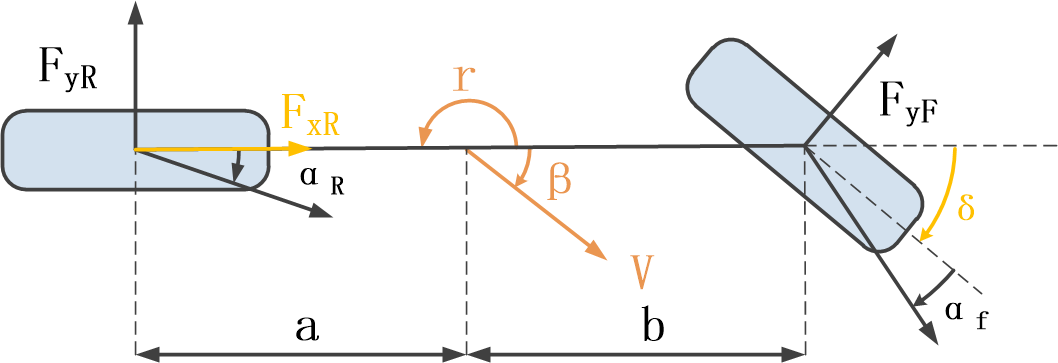
Following [4], a classic drift single-track bicycle model is applied, as illustrated in Fig. 2. Simplifying the drifting vehicle as a rigid body, the model encompasses three states : the total velocity vector with magnitude V, sideslip angle and yaw rate of the vehicle’s body r. The control variables are steering angle and rear longitudinal force . The equations of motion then are:
| (15) | ||||
| (16) | ||||
| (17) |
where m represents the mass, is the moment of inertia in the vertical direction, a and b are the distance from the center of gravity to the front and rear axle respectively. The lateral forces acting on the vehicle are the front lateral force and the rear lateral force , which are both modeled using the simplified Pacejka tire model [25]
| (18) | |||
| (19) |
where is the friction coefficient, B and C are tire parameters, is the vertical load on the tire. The front and rear tire slip angles are
| (20) | ||||
| (21) |
III-B Residual Model Learning
While the model above can reflect the vehicle dynamics to a considerable extent, there are still problems of model mismatch due to environmental interference or simplified formulas. To improve the model’s accuracy and performance, we compensate the model error from the deviation of the nominal model by utilizing GP.
Throughout the vehicle’s operation, performance data are systematically gathered . GP’s training inputs and outputs are
| (23a) | ||||
| (23b) | ||||
Due to the assumption that each dimension is uncorrelated, three independent GPs are trained (6). The stochastic vehicle model, incorporating residual compensation , is expressed as follows:
| (24) |
The performance of GP regression is highly dependent on the choice of data points. But retaining all data throughout the process will lead to computational infeasibility. So we only store the most informative data points in a dictionary [12], maintaining the dictionary size based on points distance measurement method [13].
III-C Drift Equilibrium Analysis
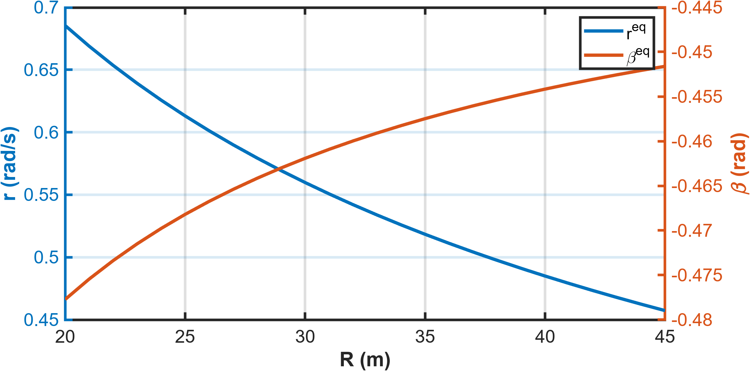
Previous works have proved the existence of a drift saddle equilibrium point [26] [27]. Drift equilibrium is a form of steady-state turning, which satisfies the formula for calculating the steady-state radius . It’s a common way to find the equilibrium point by simply setting vehicle states unchanged over control variables (i.e. ) and fixing the values for , , making the number of unknowns equal to the number of equations. For the stochastic case (24), we use the predictive mean to describe the residual part (i.e. ).
To get the equilibrium points, vehicle parameters are as follows: =1, m=1140 kg, a=1.165 m, b=1.165 m, =1020 kg, B=12.55, C=1.494. Fig 3 presents a portion of the equilibrium points derived from the nominal model (22) with =-20 deg and varying from 20 m to 45 m.
IV Drift Controller Structure
Our work focuses on steady-state drifting, aiming to maneuver the vehicle along a specific path while keeping the vehicle’s states around drift equilibrium. An illustration of the framework can be found in Fig. 1. The path tracking block is designed to provide equilibrium points for the optimal control block to follow. The optimal control block formulates a deterministic optimization problem and solves it with iLQR combined with ADMM. Throughout the process, data is collected for residual model learning with GP training (Section III-B).
IV-A Path Tracking
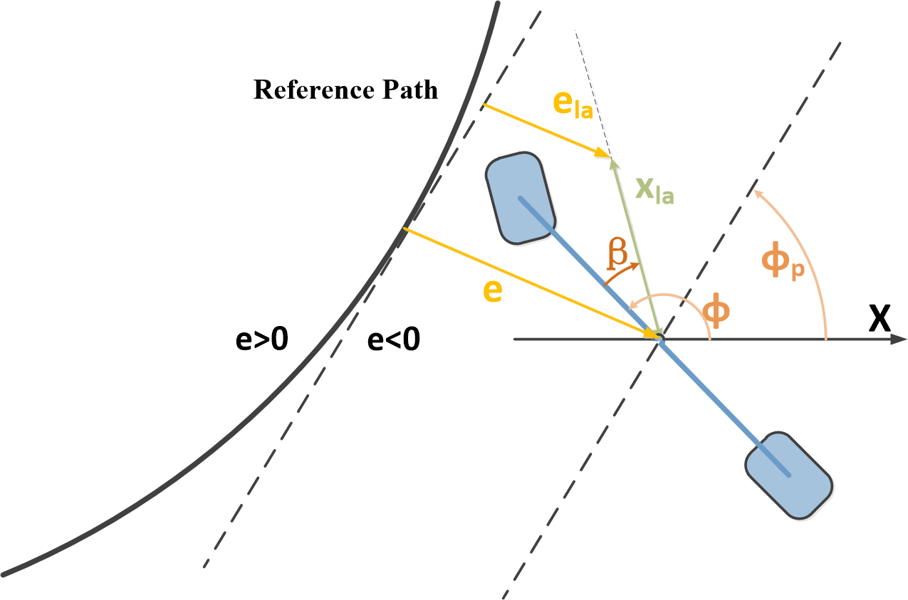
The core idea is to utilize the lateral error to adjust the desired curvature, as illustrated in Fig.4. Instead of using the instantaneous lateral error , we use the look-ahead error as the input to a PID controller. Here, represents the look-ahead distance, and denotes the course direction error, where is the vehicle’s heading angle and is the path angle. The PID controller’s output, which provides curvature compensation , is used to determine the reference curvature , where is the path curvature. With accounting for potential trajectory deviations and the PID controller converting the error into the appropriate curvature adjustments, we can achieve a balance between fast response and strong robustness against minor disturbances. The desired drift equilibrium is then achieved with the specified and a manually fixed (Section III-C)
IV-B Optimal Control
This part aims at following desired equilibrium points by solving optimal control problems.
IV-B1 Problem Formulation
Consider the following stochastic problem with control limitation and control-smoothing terms:
| (25a) | ||||
| s.t. | (25b) | |||
| (25c) | ||||
where the cost functions are in quadratic form: and . and are lower and upper limits for control variables .
Note that the learned GP model (24) has rendered states stochastic variables and states in fact are not Gaussian distributions because of the nonlinear mapping. A common approach to assess the uncertainty in these states is to approximate them as Gaussian distributions and propagate their mean and variance through successive linearizations [13]. In our experiment, we use the GP to estimate the state variances but do not propagate them as in an extended Kalman filter, in order to reduce the computational burden. The mean and variance are estimated as follows:
| (26a) | |||
| (26b) | |||
We reformulate the probabilistic problem (25) to a deterministic one by introducing the Gaussian belief augmented state vector [28] :
| (27a) | ||||
| s.t. | (27b) | |||
| (27c) | ||||
where the new cost function is defined as and the augmented dynamics are given by (26).
It is important to highlight that introducing GP can significantly increase the nonlinearity of the system. This makes the choice of a highly efficient solver critical to ensuring timely and accurate solutions. To address this, we solve the deterministic problem (27) using a numerical solver that integrates iLQR with ADMM, which notably reduces the average computation time. This approach shares a fundamental alignment with the methodology presented in [21].
IV-B2 ADMM-based iLQR
In this part, ADMM is employed to exploit the structure of (27) by decomposing the optimization problem into two manageable sub-problems: a typical unconstrained OCP and a QP problem. Firstly, we define the indicator function:
| (28) |
with respect to a set . We further define sets:
| (29) | ||||
| (30) |
By introducing the consensus variable , (27) can be transferred as:
| (31a) | ||||
| (31b) | ||||
| s.t. | (31c) | |||
Then, we can define the augmented Lagrangian function of (31) as:
| (32a) | ||||
| (32b) | ||||
| (32c) | ||||
where is a Lagrange multiplier and is a scalar penalty weight. We arrive at the three-step ADMM iteration [16] by alternately minimizing over and , rather than simultaneously minimizing over both:
| (33) | ||||
| (34) | ||||
| (35) |
The above three steps are repeated until the desired convergence tolerance is reached, with further details provided below.
The first ADMM step (33) is equivalent to solving the following problem:
| (36a) | ||||
| s.t. | (36b) | |||
with . Since the problem only involves dynamic constraints, the iLQR algorithm can efficiently solve the optimal control problem (36) without requiring an initial feasible solution.
The second ADMM step (34) is equivalent to solving the following QP problem:
| (37a) | ||||
| s.t. | (37b) | |||
A novel fast solver for QP based on Pseudo-Transient Continuation (PTC) [29] is applied for solving the above problem (37). 111[29] requires equality constraints with full row rank. To solve this problem, we introduce an additional constant variable (i.e. ) to have an equality constraint (i.e. ). Please refer to the original paper for more details.
The third ADMM step (35) is a gradient-ascent update on the Lagrange multiplier.
V SIMULATION RESULTS
The whole experiment is conducted on a joint simulation platform using MATLAB-R2023a and the high-fidelity vehicle simulation software CarSim-2019. The simulation is executed on an Intel i7-8565U processor.
V-A Simulation Setup
We selected a Clothoid curve as the reference path [4], with a radius ranging between 20 m and 45 m, as shown in Fig.5. The front wheel angle is set to -20 deg, with an initial speed of 12 m/s. The look-ahead distance is 30 m. Vehicle parameters have been illustrated in section III-C. The real friction coefficient is set to =1.
The drift controller is activated at the start of the simulation, operating independently without the help of a guide controller. In all scenarios, the prediction horizon is chosen as N = 20. The weighting parameters are established as , and . After successfully solving the optimal control problem, the results are stored and then used as the initial guess for the next timestep to facilitate warm starting.
The simulation is initialized with the nominal model, where all GP-dependent variables are initially set to zero (24). The data collected under the nominal controller is then used to populate the GP dictionary with an initial set of up to 50 data points for each dimension. After completing the first lap, the GP-enhanced dynamics (26) are employed for the subsequent 5 laps.
V-B Results
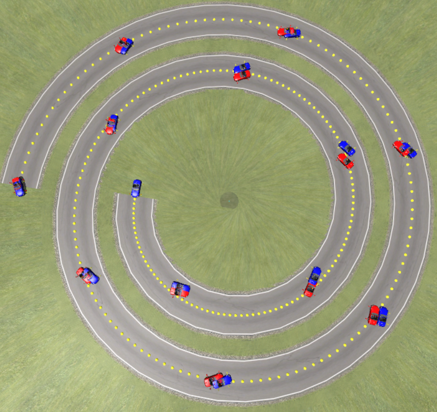
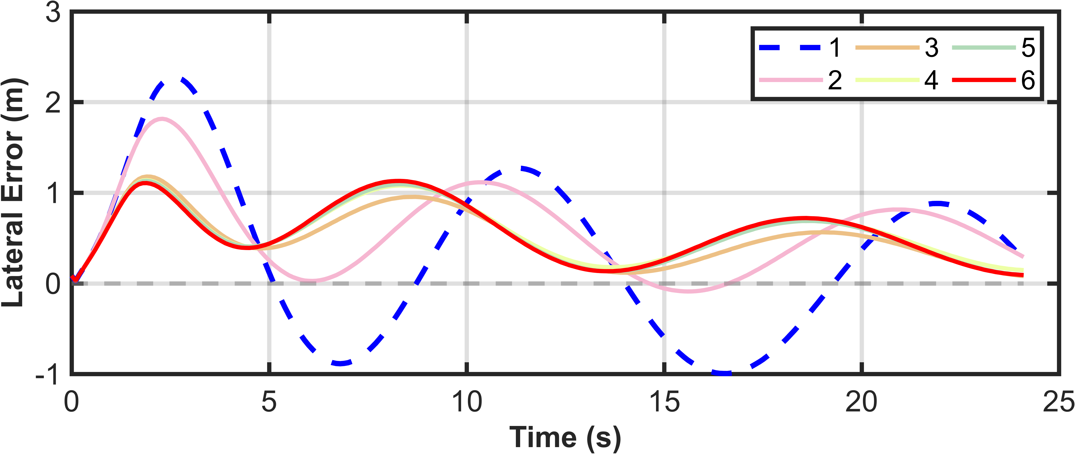
To demonstrate the trajectory tracking effectiveness of the drifting control approach, we first compare the lateral errors across successive laps, as shown in Fig.6 and summarized in Table.I. Initially, with the nominal controller, the Root Mean Square Error (RMSE) is approximately 0.94 m, and the maximum lateral error is around 2.28 m. A significant improvement is observed in lap 3, with the RMSE and maximum lateral error reduced to 0.58 m and 1.18 m respectively, constituting an improvement of almost and . The drifting trajectories for the nominal controller (lap 1) and the GP-based controller (lap 6) are illustrated in Fig 5.
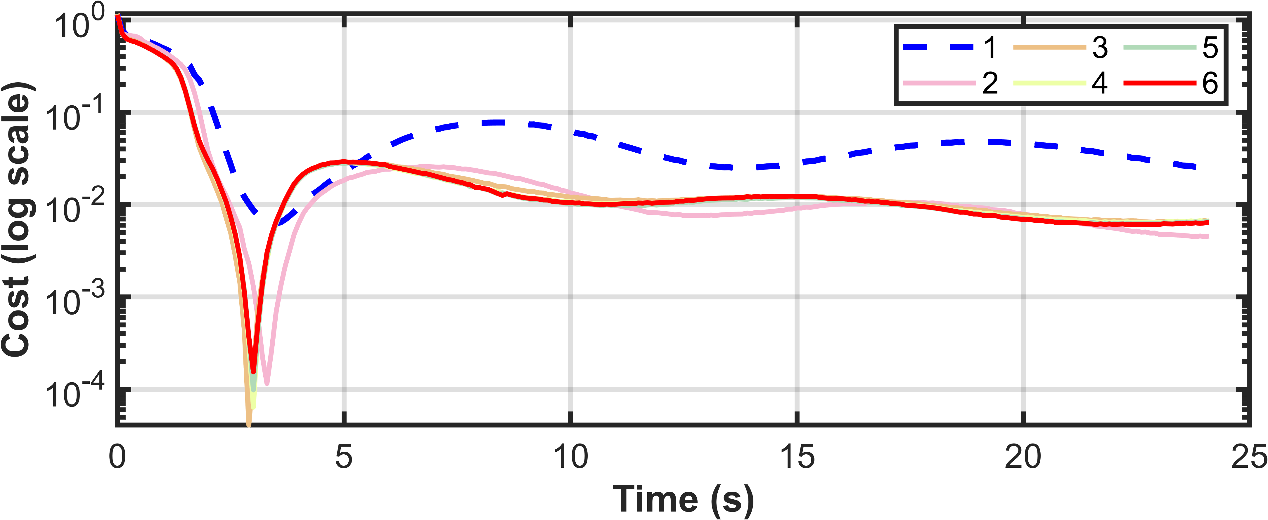
In addition, we examine the equilibrium tracking performance. It is important to note that the GP is also utilized in the drift equilibrium calculation to provide more accurate desired states. To assess how well the system tracks the changing equilibrium point, we employ a quadratic cost function . The equilibrium point tracking ability is shown in Fig 7. The GP-based controller exhibits superior equilibrium tracking performance throughout each lap, as evident by its lower cost compared to the controller without GP. And the average cost converges quickly in the subsequent laps.
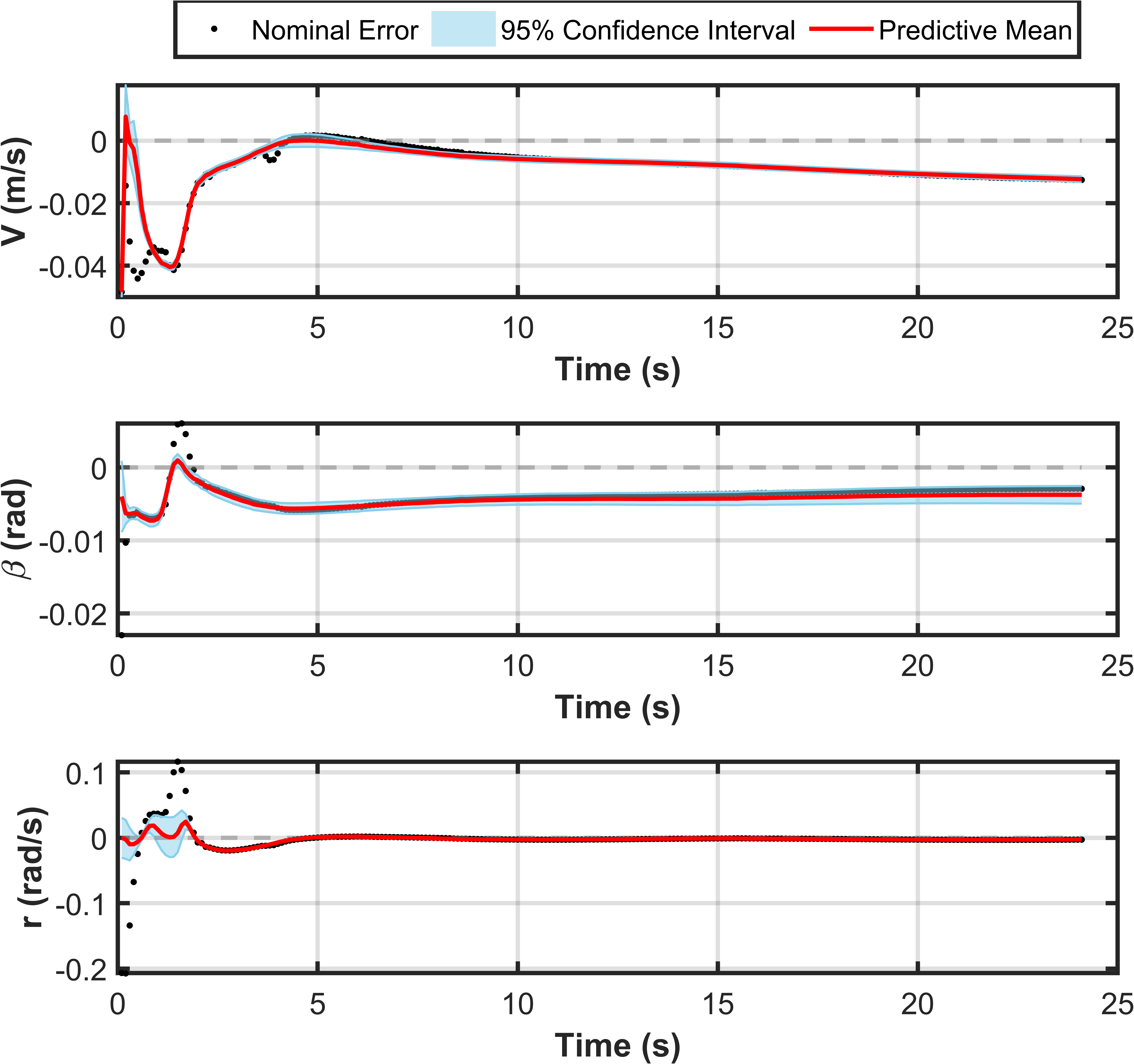
Next, the model’s learning performance is analyzed, as illustrated in Fig. 8. We present the nominal model errors encountered (i.e. errors between the measurement and nominal prediction), along with the corresponding GP compensations in the final lap. The results indicate that both the GP’s mean and uncertainty estimates align well with the true model errors. To quantify the learning performance, we define the prediction error as for the nominal controller, and for the GP-based controller. As shown in Table I, the prediction error decreased from 0.0153 at the start to 0.0059 after two rounds of learning, reflecting a reduction of approximately .
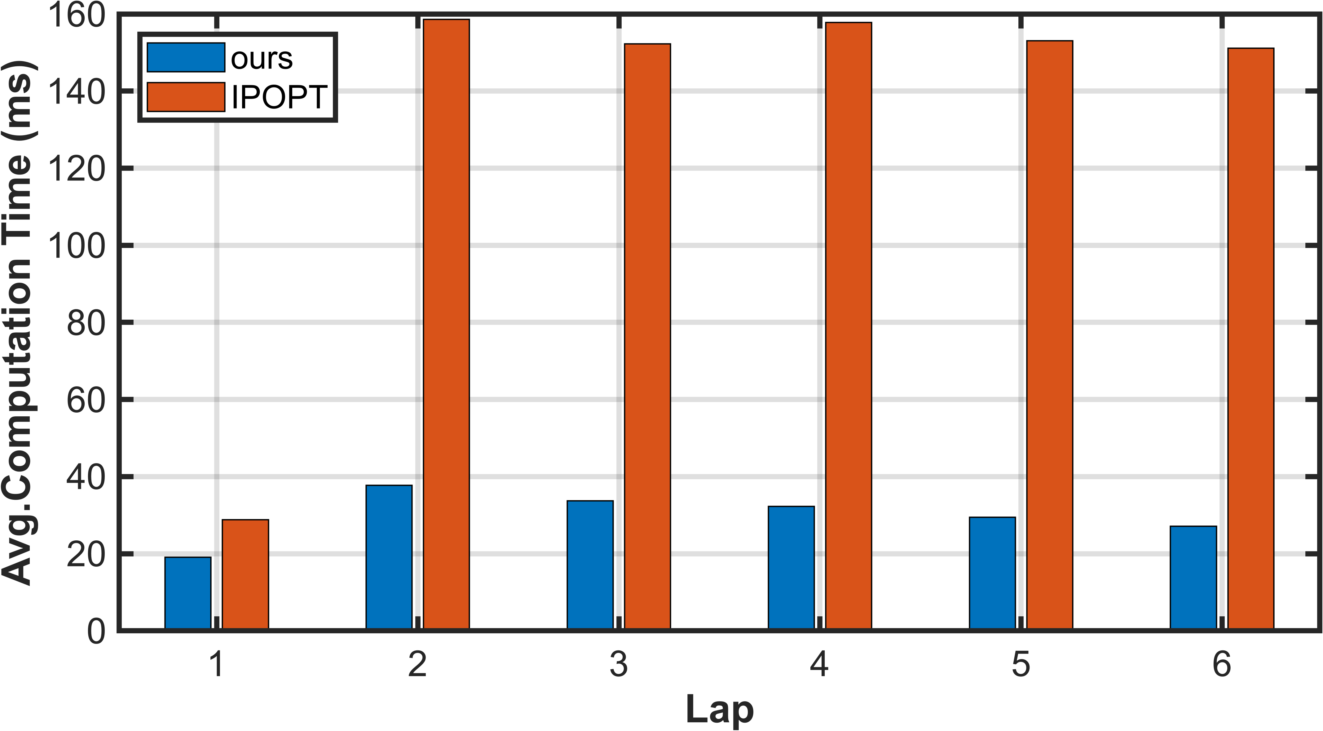
The computation time of our ADMM-based iLQR method is recorded, and comparison studies are conducted using CasADi [30], an optimization solver that utilizes IPOPT [31]. The results, shown in Fig. 9, indicate a significant increase in computation time for the IPOPT following the introduction of GP, consistently reaching around 160 ms from lap 2 onward. In contrast, our method demonstrates much lower computation time, remaining under 20 ms in lap 1 and below 40 ms in the subsequent laps. The time cost decreased about 75 from lap 2 onward. These findings highlight the strong potential of our approach for real-time applications and higher control frequency.
To rigorously evaluate the robustness of the proposed method, a 10 variation (both increasing and decreasing) in the friction coefficient was applied to simulate fluctuations in the vehicle’s operating environment. The system’s performance was systematically evaluated under these varying conditions using the established criteria. As indicated in Table I, the method consistently demonstrated high effectiveness, underscoring its robustness and adaptability across a range of dynamic conditions, thereby ensuring reliable operation.
| Metric | Lap | Friction Coefficient | ||||
|---|---|---|---|---|---|---|
| RMSE. Lateral Error (m) | 1 | 2.7652 | 1.6243 | 0.9405 | 0.8868 | 1.5080 |
| \cdashline2-7 | 2 | 1.6414 | 0.6827 | 0.7612 | 0.5187 | 1.1663 |
| 3 | 0.9084 | 0.8064 | 0.5839 | 0.5823 | 1.1190 | |
| 4 | 0.6265 | 0.9116 | 0.6412 | 0.6037 | 1.0927 | |
| 5 | 0.7392 | 0.7507 | 0.6340 | 0.5112 | 1.1138 | |
| 6 | 0.6499 | 0.7798 | 0.6436 | 0.5527 | 1.1232 | |
| Max. Lateral Error (m) | 1 | 5.3484 | 3.5088 | 2.2770 | 1.5935 | 2.7996 |
| \cdashline2-7 | 2 | 3.2196 | 1.7688 | 1.8167 | 0.9979 | 1.9847 |
| 3 | 1.8731 | 1.9754 | 1.1799 | 1.1593 | 1.9624 | |
| 4 | 1.3426 | 2.2271 | 1.1399 | 1.1968 | 1.9551 | |
| 5 | 1.6108 | 1.6994 | 1.1319 | 0.9777 | 1.9714 | |
| 6 | 1.5402 | 1.5899 | 1.1312 | 1.1302 | 1.9863 | |
| Avg. Cost | 1 | 0.5159 | 0.0999 | 0.0798 | 0.0770 | 0.0931 |
| \cdashline2-7 | 2 | 0.1124 | 0.0594 | 0.0497 | 0.0471 | 0.0605 |
| 3 | 0.0663 | 0.0562 | 0.0456 | 0.0479 | 0.0626 | |
| 4 | 0.0573 | 0.0570 | 0.0450 | 0.0483 | 0.0639 | |
| 5 | 0.0543 | 0.0491 | 0.0448 | 0.0474 | 0.0645 | |
| 6 | 0.0504 | 0.0474 | 0.0473 | 0.0503 | 0.0648 | |
| Avg. Prediction Error | 1 | 0.0428 | 0.0319 | 0.0153 | 0.0235 | 0.0471 |
| \cdashline2-7 | 2 | 0.0420 | 0.0142 | 0.0065 | 0.0086 | 0.0308 |
| 3 | 0.0298 | 0.0060 | 0.0059 | 0.0083 | 0.0296 | |
| 4 | 0.0168 | 0.0049 | 0.0060 | 0.0081 | 0.0295 | |
| 5 | 0.0067 | 0.0049 | 0.0060 | 0.0072 | 0.0296 | |
| 6 | 0.0067 | 0.0053 | 0.0060 | 0.0078 | 0.0296 | |
Note: denotes a failure to drift due to an excessively large . However, with the integration of GP, the vehicle successfully learns to drift starting from lap 2.
VI CONCLUSIONS
This work presents a novel hierarchical control framework combining GP with an ADMM-based iLQR for autonomous vehicle drift control. The integration of GP effectively compensates for model inaccuracies, significantly improving path-tracking performance. The combination of ADMM and iLQR allows for efficient problem decomposition, leading to efficient solutions. Simulation results show that our method achieves a 38 reduction in RMSE lateral error and a 75 reduction in computation time compared to IPOPT, making it highly suitable for real-time applications in dynamic environments.
Future work will focus on extending the framework to experimental validation using scaled autonomous racing cars, exploring its adaptability to real-world scenarios, and further optimizing its performance under varying environmental conditions.
ACKNOWLEDGMENT
Thanks to Bei Zhou and Xiewei Xiong for valuable suggestions.
References
- [1] B. Lenzo, T. Goel, and J. C. Gerdes, “Autonomous drifting using torque vectoring: Innovating active safety,” IEEE Transactions on Intelligent Transportation Systems, 2024.
- [2] F. Jia, H. Jing, and Z. Liu, “A novel nonlinear drift control for sharp turn of autonomous vehicles,” Vehicle system dynamics, vol. 62, no. 2, pp. 490–510, 2024.
- [3] J. Y. Goh and J. C. Gerdes, “Simultaneous stabilization and tracking of basic automobile drifting trajectories,” in 2016 IEEE Intelligent Vehicles Symposium (IV). IEEE, 2016, pp. 597–602.
- [4] J. Y. Goh, T. Goel, and J. Christian Gerdes, “Toward automated vehicle control beyond the stability limits: drifting along a general path,” Journal of Dynamic Systems, Measurement, and Control, vol. 142, no. 2, p. 021004, 2020.
- [5] C. Hu, X. Zhou, R. Duo, H. Xiong, Y. Qi, Z. Zhang, and L. Xie, “Combined fast control of drifting state and trajectory tracking for autonomous vehicles based on mpc controller,” in 2022 International Conference on Robotics and Automation (ICRA). IEEE, 2022, pp. 1373–1379.
- [6] C. Hu, L. Xie, Z. Zhang, and H. Xiong, “A novel model predictive controller for the drifting vehicle to track a circular trajectory,” Vehicle System Dynamics, pp. 1–30, 2024.
- [7] G. Bellegarda and Q. Nguyen, “Dynamic vehicle drifting with nonlinear mpc and a fused kinematic-dynamic bicycle model,” IEEE Control Systems Letters, vol. 6, pp. 1958–1963, 2021.
- [8] J. Y. Goh, M. Thompson, J. Dallas, and A. Balachandran, “Beyond the stable handling limits: nonlinear model predictive control for highly transient autonomous drifting,” Vehicle System Dynamics, pp. 1–24, 2024.
- [9] V. A. Laurense, J. Y. Goh, and J. C. Gerdes, “Path-tracking for autonomous vehicles at the limit of friction,” in 2017 American control conference (ACC). IEEE, 2017, pp. 5586–5591.
- [10] X. Zhou, C. Hu, R. Duo, H. Xiong, Y. Qi, Z. Zhang, H. Su, and L. Xie, “Learning-based mpc controller for drift control of autonomous vehicles,” in 2022 IEEE 25th International Conference on Intelligent Transportation Systems (ITSC). IEEE, 2022, pp. 322–328.
- [11] F. Djeumou, J. Y. Goh, U. Topcu, and A. Balachandran, “Autonomous drifting with 3 minutes of data via learned tire models,” in 2023 IEEE International Conference on Robotics and Automation (ICRA). IEEE, 2023, pp. 968–974.
- [12] L. Hewing, J. Kabzan, and M. N. Zeilinger, “Cautious model predictive control using gaussian process regression,” IEEE Transactions on Control Systems Technology, vol. 28, no. 6, pp. 2736–2743, 2019.
- [13] J. Kabzan, L. Hewing, A. Liniger, and M. N. Zeilinger, “Learning-based model predictive control for autonomous racing,” IEEE Robotics and Automation Letters, vol. 4, no. 4, pp. 3363–3370, 2019.
- [14] B. Zhou, H. Cheng, Y. Shi, H. Xiaorong, L. Xie, and S. Hongye, “Learning-based hierarchical model predictive control for drift vehicles,” in 2024 American Control Conference (ACC). IEEE, 2024, pp. 3524–3530.
- [15] W. Li and E. Todorov, “Iterative linear quadratic regulator design for nonlinear biological movement systems,” in First International Conference on Informatics in Control, Automation and Robotics, vol. 2. SciTePress, 2004, pp. 222–229.
- [16] S. Boyd, N. Parikh, E. Chu, B. Peleato, J. Eckstein et al., “Distributed optimization and statistical learning via the alternating direction method of multipliers,” Foundations and Trends® in Machine learning, vol. 3, no. 1, pp. 1–122, 2011.
- [17] Y. Tassa, N. Mansard, and E. Todorov, “Control-limited differential dynamic programming,” in 2014 IEEE International Conference on Robotics and Automation (ICRA). IEEE, 2014, pp. 1168–1175.
- [18] T. A. Howell, B. E. Jackson, and Z. Manchester, “Altro: A fast solver for constrained trajectory optimization,” in 2019 IEEE/RSJ International Conference on Intelligent Robots and Systems (IROS). IEEE, 2019, pp. 7674–7679.
- [19] J. Chen, W. Zhan, and M. Tomizuka, “Autonomous driving motion planning with constrained iterative lqr,” IEEE Transactions on Intelligent Vehicles, vol. 4, no. 2, pp. 244–254, 2019.
- [20] K. Nguyen, S. Schoedel, A. Alavilli, B. Plancher, and Z. Manchester, “Tinympc: Model-predictive control on resource-constrained microcontrollers,” in 2024 IEEE International Conference on Robotics and Automation (ICRA). IEEE, 2024, pp. 1–7.
- [21] J. Ma, Z. Cheng, X. Zhang, M. Tomizuka, and T. H. Lee, “Alternating direction method of multipliers for constrained iterative lqr in autonomous driving,” IEEE Transactions on Intelligent Transportation Systems, vol. 23, no. 12, pp. 23 031–23 042, 2022.
- [22] V. Sindhwani, R. Roelofs, and M. Kalakrishnan, “Sequential operator splitting for constrained nonlinear optimal control,” in 2017 American Control Conference (ACC). IEEE, 2017, pp. 4864–4871.
- [23] C. K. Williams and C. E. Rasmussen, Gaussian processes for machine learning. MIT press Cambridge, MA, 2006, vol. 2, no. 3.
- [24] Y. Tassa, T. Erez, and E. Todorov, “Synthesis and stabilization of complex behaviors through online trajectory optimization,” in 2012 IEEE/RSJ International Conference on Intelligent Robots and Systems. IEEE, 2012, pp. 4906–4913.
- [25] E. Bakker, L. Nyborg, and H. B. Pacejka, “Tyre modelling for use in vehicle dynamics studies,” SAE transactions, pp. 190–204, 1987.
- [26] C. Voser, R. Y. Hindiyeh, and J. C. Gerdes, “Analysis and control of high sideslip manoeuvres,” Vehicle System Dynamics, vol. 48, no. S1, pp. 317–336, 2010.
- [27] R. Y. Hindiyeh and J. Christian Gerdes, “A controller framework for autonomous drifting: Design, stability, and experimental validation,” Journal of Dynamic Systems, Measurement, and Control, vol. 136, no. 5, p. 051015, 2014.
- [28] Y. Pan and E. Theodorou, “Probabilistic differential dynamic programming,” Advances in Neural Information Processing Systems, vol. 27, 2014.
- [29] L. Calogero, M. Pagone, and A. Rizzo, “Enhanced quadratic programming via pseudo-transient continuation: An application to model predictive control,” IEEE Control Systems Letters, 2024.
- [30] J. A. E. Andersson, J. Gillis, G. Horn, J. B. Rawlings, and M. Diehl, “CasADi – A software framework for nonlinear optimization and optimal control,” Mathematical Programming Computation, vol. 11, no. 1, pp. 1–36, 2019.
- [31] A. Wächter and L. T. Biegler, “On the implementation of an interior-point filter line-search algorithm for large-scale nonlinear programming,” Mathematical programming, vol. 106, pp. 25–57, 2006.