A High-Speed Time-Optimal Trajectory Generation Strategy via a Two-layer Planning Model

Abstract

Motion planning and trajectory generation are crucial technologies in various domains including the control of Unmanned Aerial Vehicles (UAV), manipulators, and rockets. However, optimization-based real-time motion planning becomes increasingly challenging due to the problem’s probable non-convexity and the inherent limitations of Non-Linear Programming algorithms. Highly nonlinear dynamics, obstacle avoidance constraints, and non-convex inputs can exacerbate these difficulties. To address these hurdles, this paper proposes a two-layer optimization algorithm for 2D vehicles by dynamically reformulating small time horizon convex programming subproblems, aiming to provide real-time guarantees for trajectory optimization. Our approach involves breaking down the original problem into small horizon-based planning cycles with fixed final times, referred to as planning cycles. Each planning cycle is then solved within a series of restricted convex sets identified by our customized search algorithms incrementally. The key benefits of our proposed algorithm include fast computation speeds and lower task time. We demonstrate these advantages through mathematical proofs under some moderate preconditions and experimental results.

¹, ²

1 Introduction

As industrial technology continues to evolve, numerous automobile devices have emerged, giving rise to trajectory generation as a vital realm of research. Trajectory generation and motion planning aim to find proper control for agents such as robots, drones, or other autonomous systems to navigate from one location to another while avoiding obstacles. An efficient trajectory planning method is essential to successful applications ranging from mobile robots in warehouses to autonomous vehicles in complex urban environments. A proper controller can significantly benefit these applications by saving energy and minimizing harm to motor systems, ultimately resulting in substantial financial savings. Over the past few decades, a variety of planning algorithms have emerged. Despite their differing methodologies and distinct application scenarios, these methods can be broadly categorized into three primary categories [1]: The search-based methods, the sampling-based and the optimization-based ones.

A well-known search-based algorithm is A* which first introduced by Peter Hart, Nilsson and Bertram Raphael in 1968 [2]. By introducing two heuristic functions, the A* algorithm shows its effectiveness [3] as long as the designer properly adjusts the heuristic functions [4][5][6]. However, with the intricacy demerits of A*, when the reachable area becomes larger or the grid division gets denser, the A* algorithm needs to search for a huge number of nodes, resulting in a high computation time cost and efficiency reduction [7]. At the same time, a large dataset also requires significant storage space, which is undesirable in online-computation devices [8]. As an upgraded version of A*, the dynamic A* algorithm, D*, is proposed to improve the robustness [9], and the main difference between A* and D* originates from their dynamic performances. If an obstacle undesirably appears on the waypoint after planning and calculating, D* will just revise the infeasible path segments, while the rest of path remains. By dynamically detecting and replanning, the D* algorithm ensures the immediate validity of the path. Similar to D*, ARA* [10] is an algorithm applied to improve the quality of the generated paths. During the optimization process, the ARA* algorithm reuses previous search results to make it more effective than A*. However, A* and its improved versions cannot essentially reduce the computational burden, hence they are difficult to be applied in large-scale real-time problems.

For sampling-based algorithms, a famous setup is the rapid random trajectory (RRT) method. Initialized by J. J. Kuffner and Steven M. La Valle [11], this kind of algorithm is widely used in obstacle avoidance tasks due to its easiness and flexibility by constructing space-filling trees to search a feasible path [12][13][14]. To further enhance the optimality, RRT* [15] with a higher computation bundle is further introduced. Since these planning algorithms are well applied in distinct scenarios, there are vast variations of RRT with incomparable advantages in specific scenarios [16][17]. However, due to the limitation of hardware, it is also challenging to apply RRT-type algorithms in some real-time systems. In addition, to the best of our knowledge, the RRT-type algorithms generally calculate paths that are independent of the time parameters. Although the generated paths effectively circumvent obstacles in space, they may fail to meet the kinematic constraints, i.e., no feasible control inputs allow the agent to travel along the predetermined path.

During the past few decades, there are also vast studies that tackle planning problems with optimization techniques. Sometimes, the planning problem itself can be profiled with simple models. In this case, an ideal closed-form control input may be generally obtained by indirect methods under Pontryagin’s maximum principle [18] or Lagrangian multiplier method [19]. Although indirect methods are analytical and accurate, they are not easy to calculate by computer devices and the solution is prone to change concerning the initial guess. In contrast, the direct methods discretize the original problem, and convert the optimal control to a nonlinear programming problem (NLP), then solve it by optimization methods such as the newton method [20], ADMM [21] or genetic algorithm. Although the NP-hard state of general nonlinear problems has been a mutual challenge, it has been shown that some specific problems can be transformed to convex ones, thus reducing the difficulty thanks to previous studies. In this way, it has become a hot topic to study how to reconstruct a prevalent non-convex problem into the convex setups, and the approaches are generally classified into one-shot methods, which obtain the trajectory all at once with only one reconstructed problem and sequential optimization algorithms [22]. For some non-convex inputs such as the positive minimal thrust constraints in the rocket model, we can apply the lossless convex relaxation technique to broaden the original control vector such that the non-convex input constraints are transformed into convex ones while lifting the dimension of the problem [23][24][25]; despite the extra variables being introduced, the relaxed problems become easier to solve from its convex structure, and at the same time, formal proof is provided to show the feasibility of lossless convexification under some assumptions. For problems with non-convex states such as maps with obstacle-avoidance constraints, sequential optimization algorithms can be applied to find a feasible trajectory quickly [28]. In these methods, a reference trajectory (not necessarily feasible) is required initially, then linearize or quadratize the non-convex objective function according to the reference trajectory, while relaxing or tightening the non-convex constraint set at the same time to obtain a convex subproblem. An optimal trajectory of the subproblem will be used as the warm-start reference trajectory for the next subproblem, back and forth until the solution converges under a given tolerance. Sequential optimization methods generally do not solve the original problem all at once, and it may result in obtaining an error solution by some factors during iterations [22]. For instance, if the convexified state constraints are relaxed, the generated trajectory may be out of the original constraints; if the intersection of all the approximated constraints is empty, one subproblem will get into an error that can interrupt the iteration. Moreover, the optimal solution of a subproblem may be boundless if the convexified costs are linear while the constraint sets are boundless. These factors are undesirable while chronically happening. After all, sequential optimization methods are not a universal approach either. To mitigate these shortcomings, some variations of sequential optimization methods have been invented. To handle the probable unboundedness, a trust region constraint can be added, or introduce penalty functions to make the original problem quadratic. On the other hand, using stricter approximated constraints and transferring the hard constraints to soft ones can reduce the risk of illusory solutions and alleviate the so-called artificial infeasibility respectively [29].

Direct optimization methods are also widely employed in time-optimal control problems. The modelling process for fixed-time step problems is relatively straightforward, which enables us to transform free final time problems into a series of fixed-final time optimization subproblems, and a line search program can be applied to obtain a proper trajectory from the solution of those subproblems [30]. Time-optimal control problems can also be settled by solving fixed-time optimal subproblems successively [31]. However, this approach relies heavily on the availability of extensive map information and lacks final constraints, which may limit its applicability.

This paper focuses on a collision-free trajectory generating problems with static or moving obstacles. In order to improve the quality and time optimality of the solutions in motion planning, we propose a dynamic trajectory generation algorithm that is rooted in an iterative two-layer optimization procedure. In each iteration, a planning cycle featuring a short fixed final time is employed, with each cycle further divided into two trajectory optimization problems and an associated trajectory searching algorithm. By incrementally generating segmented control inputs, an entire control can be obtained with dynamic obstacle avoidance capability. Moreover, for the aforementioned trajectory searching step, we provide two corresponding trajectory searching algorithms and discuss their feasibility. The contents and contribution of this paper are as follows.

• We apply trajectory searching methods to effectively generate restricted convex areas with the help of nominal trajectories, thereby mitigating non-convexity while ensuring feasibility. Moreover, a customized artificial potential field method with kinematic reliability is suggested as a trajectory-searching algorithm. The customized artificial potential field approach can further be applied independently as a planning algorithm;

• Our proposed algorithms have been rigorously proven to produce trajectories with approximated optimal local minimal final time under specified conditions and moderate assumptions;

• By decomposing the complete problem into planning cycles and solving one planning cycle in parallel mode while moving, we have developed a robust framework for safe navigation in dynamic environments featuring movement obstacles, which ensures both reliability and precision while only relying on a part of map information.

In the remainder of this paper, we organize our content logically and coherently. The optimal control problem is formulated in Section II, providing a clear foundation for further analysis. In Section III, we introduce the two-layer model and develop trajectory searching algorithms, then thoroughly analyse them to demonstrate their effectiveness. Subsequent Section IV presents numerical experiments that utilize both static and dynamic maps, allowing us to present the conclusions in Section V.

2 Problem Formulation

In this section, we provide necessary annotations to ensure clarity and consistency throughout the paper. All the sets are discussed in Euclidean space $\mathbb{R}^{n}$ with $n$ specialized case by case and with the norm $\left\|{\mathbf{a}}\right\|=\sqrt{\left\langle{\left.{{\mathbf{a,a}}}\right\rangle}\right.}=\sqrt{{{\mathbf{a}}^{\top}}{\mathbf{a}}}$, and we further let $\|\mathbf{a}\|_{Q}=\sqrt{\mathbf{a}^{\top}Q\mathbf{a}}$ with $Q\succ 0$. We also define sliced vectors, denoted by $\mathbf{a}[i:j]$, which consists of row $i$ to row $j$ from column $\mathbf{a}$. For instance, if $\mathbf{a}=[a_{1},a_{2},a_{3},a_{4}]^{\top}$, then $\mathbf{a}[2:3]=[a_{2},a_{3}]^{\top}$. For a differentiable function $f(\mathbf{x})$ with $\mathbf{x}\in\mathbb{R}^{n}$, we represent its gradient as $\nabla f(\mathbf{x})$, which is defined by ${\left[{\frac{{\partial f}}{{\partial{x_{1}}}},\frac{{\partial f}}{{\partial{x_{2}}}},\cdots,\frac{{\partial f}}{{\partial{x_{n}}}}}\right]^{\top}}$. Moreover, the Euclidean norm of objects’ velocity is referred to as speed in this paper.

2.1 Obstacle Avoidance Constraints

Generally, trajectory generation problems aim to provide feasible and safe trajectories for vehicles or other moving agents. In a trajectory generation problem, the vehicle is required to move in a specific space, which normally includes obstacles, a target state (or target area) and an initial state. This space is referred to as map, and we denote it by $\mathcal{M}$. Since each obstacle can be considered as a subset of $\mathcal{M}$, we can represent the spaces occupied by the $i$th obstacle as $\mathcal{O}_{i}$, with the relationship shown as

$$\mathcal{O}_{i}\subset\mathcal{M}\ ,\ i\in\{1,2,\cdots,n_{obs}\}{\color[rgb]{0,0,1},}$$ (1)

with $n_{obs}$ the number of obstacles. Without losing generality, we consider $\mathcal{M}$ as an unbounded map. We further denote the occupied space by the vehicle as $\mathcal{V}$, then we have $\mathcal{V}\subset\mathcal{M}$. Throughout the entire task, no collision is allowed at any point in time. The corresponding constraints can be mathematically expressed as

$$\mathcal{O}_{i}\bigcap\mathcal{V}=\emptyset\ ,\ i\in\{1,2,\cdots,n_{obs}\}.$$ (2)

However, for irregularly shaped $\mathcal{O}_{i}$, it is difficult to analytically profile them, which poses a significant challenge in subsequent works. For simplicity, we apply

$${{\mathcal{O}}_{i}}\subseteq{\mathcal{B}}({p_{i}},{D_{i}}/2)={{\mathcal{B}}_{i}}$$ (3)

and

$${\mathcal{V}}\subseteq{\mathcal{B}}(x,{D_{v}}/2)={{\mathcal{B}}_{\mathcal{V}}}$$ (4)

as the approximated obstacles. In (3) and (4), $\mathcal{B}(p,R)$ denotes a closed ball with the centre at $p$ and the radius $R$. $D_{i}$ and $D_{v}$ are the diameter of the obstacles and vehicles, respectively, with the diameter of set $A$ being

$${D_{A}}=\left\{\begin{array}[]{l}0\hfill(A=\emptyset);\\ \sup\{y-x:x,y\in A\;,A\subseteq{\mathcal{M}}\}\hfill(else).\end{array}\right.$$ (5)

Thus, an approximated map can be created by substitute $\mathcal{O}_{i},\mathcal{V}$ with $\mathcal{B}_{i},\mathcal{B}_{v}$. In the approximated map, we do not need to consider the prior knowledge of the object shape, which greatly simplifies the design of subsequent algorithms. As a result, the obstacle avoidance constraints can be further represented as

$$\|x-p_{i}\|\geq\frac{D_{i}+D_{v}}{2}=r_{i},$$ (6)

where $x=[x_{1},x_{2}]^{\top}$ denotes the center position of $\mathcal{B}_{\mathcal{V}}$. The shape approximation scheme relies on two critical assumptions which is given by Assumptions 1 and 2 below.

Assumption 1.

Given the map, the initial and target positions are excluded out of $\mathcal{B}_{i}$ for $i\in\{1,2,\cdots,n_{obs}\}$.

Assumption 2.

For any pair of indices $i$ and $j$ with $1\leq i,j\leq n_{obs}$ and $i\neq j$, the spaces occupied by obstacles are disjoint. Moreover, it is assumed that there exists a positive constant $\ell$ with

$${\mathcal{B}}({p_{i}},{r_{i}}+0.5\ell)\cap{\mathcal{B}}({p_{j}},{r_{j}}+0.5\ell)=\emptyset,$$

for $i,j\in\{1,2,\cdots,n_{obs}\}$ and $i\neq j$.

Assumption 1 is critical because it establishes the feasible condition for tackling the original problem with the proposed algorithm. On the other hand, Assumption 2 presents a more permissive condition. This leniency can be interpreted by the fact that several small obstacles, along with their gaps, can be merged into a single large obstacle, as depicted in Fig.1. Therefore, it is evident that Assumption 2 is relatively mild.

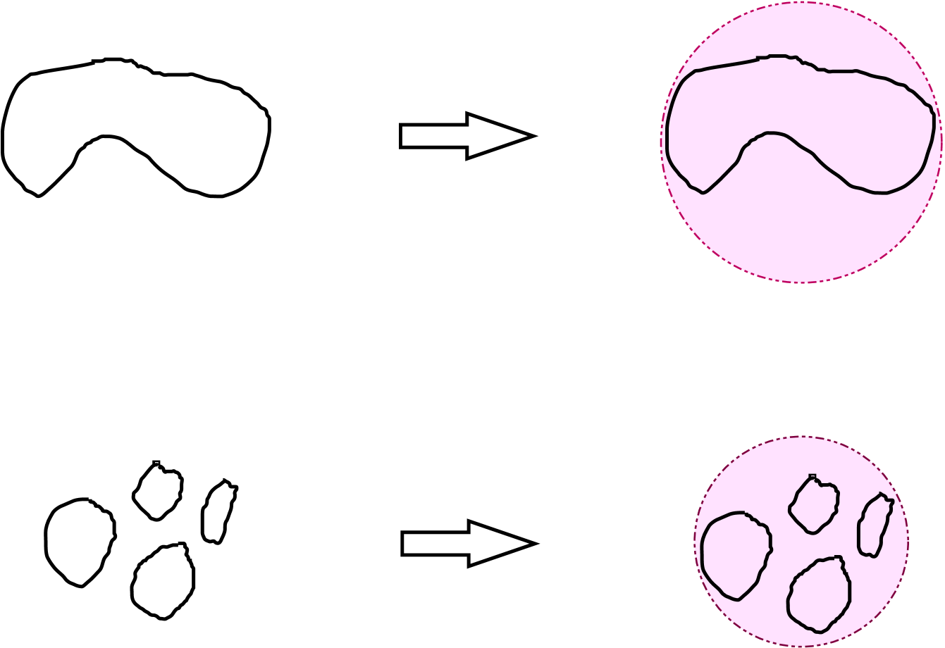
Figure 1: A single irregular obstacle (top left) could be approximated as a closed ball (top right), while multiple dense small obstacles (bottom left) could merge into a large one (top right pink circle) in consideration.

2.2 Dynamics and Objective Function

We model the map and the dynamic equation in a unified Euclidean world coordinate system. In formulating the dynamic equation, we initially consider a linear model where the acceleration serves as the input. This consideration enables us to effectively depict the dynamic function in its most basic form as

$$\dot{z}(t)=A^{\prime}z(t)+B^{\prime}u(t)+w^{\prime}(t),$$ (7)

where

$$A^{\prime} ={\begin{bmatrix}0&\hskip 10.0pt0&\hskip 10.0pt1&\hskip 10.0pt0\\ 0&\hskip 10.0pt0&\hskip 10.0pt0&\hskip 10.0pt1\\ 0&\hskip 10.0pt0&\hskip 10.0pt0&\hskip 10.0pt0\\ 0&\hskip 10.0pt0&\hskip 10.0pt0&\hskip 10.0pt0\end{bmatrix}},$$

$$B^{\prime} ={\begin{bmatrix}0&\hskip 10.0pt0&\hskip 10.0pt1&\hskip 10.0pt0\\ 0&\hskip 10.0pt0&\hskip 10.0pt0&\hskip 10.0pt1\end{bmatrix}}^{\top}.$$

The state vector $z$ is defined as the concatenation of the position vector ${x}$ and its time derivation as $z=[x^{\top},\dot{x}^{\top}]^{\top}$. If a nonlinear dynamic model is considered, for instance, the well-known Ackermann model, the corresponding dynamic function can be generally expressed as

$$\mathbf{\dot{z}}(t)=\mathbf{F}(\mathbf{z},\mathbf{u},t).$$

In this nonlinear case, an approximated linear model with the same form as (7) can be obtained by calculating the Jacobi matrix as

$$A^{\prime}={\left.{\frac{{\partial{\bf{F}}}}{{\partial{\bf{z}}}}}\right|_{{\bf{z}}={\mathbf{z}^{\prime}}}},B^{\prime}={\left.{\frac{{\partial{\bf{F}}}}{{\partial{\bf{u}}}}}\right|_{{\bf{u}}={\mathbf{u}^{\prime}}}},$$

$$w^{\prime}={\bf{F}}-{\left.{\bf{F}}\right|_{{\bf{z}}={\mathbf{z}^{\prime}},{\bf{u}}={\mathbf{u}^{\prime}}}}.$$ (8)

Remark 1.

It is well established that under most of the modelling frame, the dynamic equations are nonlinear. Although we can treat them as affine models by leveraging (8) as long as the dynamic functions are continuously differentiable, it loses precision and even results in generating fault solutions if the planning horizon considered is too long. Fortunately, we can treat the planning horizon as a “trust region”. In other words, the precision of the solution can be preserved if the linearized model is applied only in problems with small final times, which provides plausibility to the application of model linearization. Our algorithm only considers a limited horizon within each planning cycle, which enables us to handle nonlinear models in a correct manner.

The physical constraints of the vehicle can be represented as

$$0\leq\|v(t)\|\leq v_{\max}$$

and

$$0\leq\|\mathbf{u}(t)\|\leq a_{\max}.$$

These constraints can be further reformulated as $z^{\top}Q_{1}z\leq 1$ and $u^{\top}Q_{2}u\leq 1$. It is worth noting that although the probably max-speed of the vehicle is bounded by the motor’s power or other factors such as fraction, the scalar $v_{\max}$ can be chosen under the value of the probably maximal speed for the consideration of safety. A lower $v_{\max}$ tends to improve the successful rate, while a bigger $v_{\max}$ ensures a smaller time cost.

Take $z_{0}$ and $z_{f}$ as the initial and target state respectively, the boundary constraints can then be formulated as

$$z(0)=z_{0},$$ (9)

$$\|z(t_{f})-z_{f}\|_{Q_{0}}\leq\gamma{\color[rgb]{0,0,1},}$$ (10)

where $Q_{0}$ is a positive definite weight matrix, $t_{f}$ denotes the final time profiling the task’s time cost, $z(t_{f})$ is the ending state and (10) profiles the target area.

Our main goal is to drive the vehicle to the target area with a possibly low time cost. Although this can be considered a time-optimal control problem, the task’s time cost is unnecessary to consider just yet. Instead, we adopt the cost function as

$$J=[z_{f}-z(t_{f})]^{\top}Q_{0}[z_{f}-z(t_{f})],$$ (11)

Under this model frame, the trajectory can meet (10) if a sufficient big $t_{f}$ is given under Assumptions 1 & 2, and the continuous model is controllable.

2.3 Discretization and Transformation

Since it is not easy to solve continuous optimal control problems on computation devices, it is advised to convert the problem to discrete ones by shooting or other parameterization methods. In the discretization step, we substitute $z(t)$ by $\{z_{1},z_{2},\cdots,z_{N+1}\}$ and $u(t)$ by $\{u_{1},u_{2},\cdots,u_{N}\}$, then the constraints can be reformulated as

$$z_{i+1}-z_{i}=h_{i}(A^{\prime}z_{i}+B^{\prime}u_{i}+w^{\prime}_{i})\ \ i=\{1,2,\cdots,N\}.$$ (12)

In (12), $h_{i}$ represents the step lengths, which can be either constants or adapt to environmental changes. In this paper, we fixed the step length $h_{i}=h$ as a constant. Thus, it allows us to rewrite (12) to (13) as

$$z_{i+1}=Az_{i}+Bu_{i}+w_{i},$$ (13)

while a necessary assumption is critical to further analysis which is presented in Assumption 3.

Assumption 3.

In (13), $(A,B)$ is controllable and $B$ is of full column rank.

Similar to (13), two inequalities are formulated to represent discretized physical constraints, which can be represented as

$$G_{1}(z_{i})=z_{i}^{\top}Q_{1}z_{i}-1\leq 0,$$ (14)

$$G_{2}(u_{i})=u_{i}^{\top}Q_{2}u_{i}-1\leq 0.$$ (15)

The initial condition in the discretized problem can be reformulated as

$$z_{1}=z_{0}{\color[rgb]{0,0,1},}$$ (16)

while the converted boundary condition is

$$\|z_{N+1}-z_{f}\|_{Q_{0}}\leq\gamma{\color[rgb]{0,0,1}.}$$ (17)

The obstacle avoidance constraints can be further discretized as

$$\|z_{i}[1:2]-p_{j}\|\geq r_{j}$$ (18)

with $i\in\{1,2,\cdots,N+1\}$ and $j\in\{1,2,\cdots,n_{obs}\}$. Note that (18) is the sole non-convex constraint in the discretized problem, and serves as a key shorthand for general optimization-based motion planning controller operating in real-time tasks.

For the discretization of the cost function, we can rewrite (11) as

$$J=[z_{f}-z_{N+1}]^{\top}Q_{0}[z_{f}-z_{N+1}].$$ (19)

After all, given the time step $h$ and problem size $N$, the discrete formulation of the planning problem can be represented as

$$\min\eqref{J_P_1},$$

$$\mathrm{s.t.\ }\eqref{c2d_var}-\eqref{nonconvex_position_con_discrete},$$

where we denote it by $\mathcal{P}_{1}$. For the sake of convenience, if (17) is not considered in $\mathcal{P}_{1}$, a relaxed version of $\mathcal{P}_{1}$ is then constructed, and we denote the relaxed problem by $\mathcal{P}_{1}^{\prime}(z_{0})$.

Remark 2.

(12) and (13) use Euler method to approximate a derivation. Exactly, one can obtain a more precise approximation by setting

$$A =\exp(A^{\prime}h),$$

$$B =\int_{0}^{h}{\exp(A^{\prime}\tau){\rm{d}}}\tau\cdot B^{\prime},$$

and

$$w_{i}=\int_{0}^{h}{\exp(A^{\prime}\tau){\rm{d}}}\tau\cdot w^{\prime}(ih).$$

Although various discretization methods can be applied, one critical property is that $z_{i+1}-z_{i}$ owns the same order as $h$. This property is vital in subsequent algorithm analysis.

3 Algorithm Analysis

Generally, problem $\mathcal{P}_{1}$ may be solved using nonlinear programming algorithms or by convex optimization solvers iteratively via sequential convex programming (SCP). These approaches can be further categorized into one-shot and multi-step methods. The former involves solving a single problem to obtain the desired trajectory with tools like $\mathtt{LCvx}$, whereas the latter entails iteratively calculating subproblems until the convergence is achieved. These methods are almost mature while predicting computation time and solution quality for general NLP solvers remain challenging due to some inherent difficulties in their basic algorithm. For instance, SCP is susceptible to artificial infeasibility, where the infeasibility arises from over-constrained subproblems. The SCP algorithms may also produce ill solutions if some subproblems are improperly constructed, highlighting the need for careful parameter tuning and initial reference trajectory selection. Compared with these general approaches, our method is too based on convex programming to guarantee low computational time. By synthesizing control inputs dynamically, an approximated time-optimal solution can be obtained although time-optimality is not considered in the cost function. Furthermore, our algorithm definitively solves the problem within stricter convexified constraint sets, guaranteeing the feasibility of the solution far more effectively than general SCP algorithms. In the rest of this section, we will propose our trajectory generation method with analysis. Firstly, two necessary alternated problems are formulated.

3.1 Unconstrained Problem

We denote $\mathcal{P}_{w}(z_{0})$ as a relaxed version of $\mathcal{P}_{1}^{\prime}(z_{0})$, where (17) and all the non-convex obstacle avoiding constraints (18) are removed. Thus, $\mathcal{P}_{w}(z_{0})$ can be constructed as

$$\min\eqref{J_P_1},$$

$$\mathrm{s.t.\ }\eqref{c2d_var}-\eqref{initial_condition_discrete}.$$

Both the feasibility and the convexity of $\mathcal{P}_{w}(z_{0})$ are ensured for given $N$ and $h$ since (17) is not considered in this problem. Consequently, we can solve this problem to obtain a nominal trajectory, which is presented as

$$S(\mathcal{P}_{w})=\arg\min\mathcal{P}_{w}=\{\bar{z}_{1},\cdots,\bar{z}_{N+1};\bar{u}_{1},\cdots,\bar{u}_{N}\}.$$

3.2 Strict Problem

The strict problems generate trajectories within more tightly constrained feasible sets, which grant the name. The formulation of the strict problem depends on a feasible trajectory and the nominal trajectory of $\mathcal{P}_{w}(\cdot)$. Suppose $F:{\{\tilde{z}_{1},\cdots,\tilde{z}_{N+1};\tilde{u}_{1},\cdots,\tilde{u}_{N}\}}$ is aforementioned feasible trajectory of $\mathcal{P}_{1}^{\prime}$ with $\tilde{z}_{1}=\bar{z}_{1}=z_{0}$. Since $\tilde{z}_{i}[1:2]$ are collision-free points, it is easy to find a vector $\lambda_{\min}=\{\lambda_{\min,1},\lambda_{\min,2},\cdots,\lambda_{\min,N+1}\}$ with

$$\lambda_{\min,i}=\min\{\max\{\lambda_{i}:\exists p_{j},r_{j},\|z_{i}[1:2]-p_{j}\|=r_{j}\},0\},$$

where $(\lambda\tilde{z}_{i}+(1-\lambda)\bar{z}_{i})[1:2]$ are collision-free locations for any $\lambda$ with $(0<\lambda_{\min,i}<\lambda<1)$. Furthermore, we can easily derive the fact that $[\lambda_{\min}\tilde{z}+(1-\lambda_{\min})\bar{z}][1:2]$ lies on the edge of one obstacle near to $F$. Thus, some convex sets can be extracted from the original problem by

$$\mathcal{Z}_{i}=\{z_{c}|z_{c} =(1-\lambda_{\min,i}+\lambda_{f,i}-\lambda_{\min,i}\lambda_{f,i})\bar{z}_{i}$$

$$+(\lambda_{\min,i}+\lambda_{f,i}-\lambda_{\min,i}\lambda_{f,i}-\lambda_{d,i})\tilde{z}_{i}$$

$$+\lambda_{d,i}\tilde{z}_{i-1},0\leq\lambda_{d,i}\leq\lambda_{f,i}\leq 1\},$$ (20)

for $i=\{2,3,\cdots,N+1\}$. The above sets profile a triangle area in the map. Specifically, to maintain the consistency, define

$$\mathcal{Z}_{1}=\{z_{c}|z_{c} =(1-\lambda_{\min,1}+\lambda_{f,1}-\lambda_{\min,1}\lambda_{f,1})\bar{z}_{1}$$

$$+(\lambda_{\min,1}+\lambda_{f,1}-\lambda_{\min,1}\lambda_{f,1}-\lambda_{d,1})\tilde{z}_{1}$$

$$+\lambda_{d,1}\tilde{z}_{1},0\leq\lambda_{d,1}\leq\lambda_{f,1}\leq 1\}.$$ (21)

Although the convexity of these extracted sets are guaranteed, the non-feasibility may remain. To further ensure the feasibility, linear inequality constraints on $\lambda_{f,i},\lambda_{d,i}$ are introduced as

$$\lambda_{d,i}\leq k_{i}\lambda_{f,i}.$$ (22)

(22), $k_{i}$ are pre-selected to keep the convexified area out of obstacles. We denote the strict problem as $\mathcal{P}_{s}(z_{0})$, which can be presented as

$$\mathop{\min}\limits_{\{{\lambda_{f}},{\lambda_{d}}\}}{{J_{s}}({\lambda_{f}},{\lambda_{d}};\rho)}=J(z(\lambda_{f},\lambda_{d}),u(\lambda_{f},\lambda_{d}))$$

$$+\rho\cdot\|z_{0}-z_{f}\|\|\lambda_{f}-\mathbf{1}\|^{2},$$ (23)

$$\mathrm{s.t.\ }0\leq\lambda_{f,i}\leq 1,$$ (24)

$$\eqref{c2d_var},\eqref{DQ_1},\eqref{DQ_2},\eqref{initial_condition_discrete},\eqref{constraint_di}.$$

In (23), we denote $\lambda_{f}=(\lambda_{f,1},\lambda_{f,2},\cdots,\lambda_{f,N+1})^{\top}$, $\lambda_{d}=(\lambda_{d,1},\lambda_{d,2},\cdots,\lambda_{d,N+1})^{\top}$. Moreover, note that (22) and (24) are equivalent reformulation of

$$z_{i}[1:2]\in\mathcal{Z}_{i}[1:2].$$ (25)

Although $\mathcal{P}_{s}$ is feasible, its solution generally violates (17) since a small planning horizon is given to guarantee precision and reliability. To handle this difficulty, our algorithm solves $\mathcal{P}_{s}$ iteratively with planning cycles and dynamically updating relative parameters to get out of this dilemma. This manner also maintains the quality of the trajectory. Algorithm 1 uses pseudo code to depict the strategy of our proposed two-layer programming model. Throughout the entire planning process, some specific challenges may arise, which we define as connective infeasibility as Definition 1 represents.

Definition 1.

During the planning process, if an extreme $z_{N+1}$ is obtained, i.e. $z_{N+1}[1:2]$ locates very close to an obstacle, and it tends to move ahead of the obstacle with a high speed, infeasibility may arise in the subsequent planning cycle. This phenomenon is referred to as connective infeasibility.

To mitigate the connective infeasibility, $\rho\|\lambda_{f}-\mathbf{1}\|$ is introduced in $\mathcal{P}_{s}(z_{0})$ to enhance the robustness where it is referred to as the safety term.

Algorithm 1 Online Programming Algorithm

1: Input: The map information $\mathcal{M}$.

2: $K\leftarrow 1$;

3: while $\|z_{N^{(K)}+1}^{(K)}-z_{f}\|_{Q_{0}}\geq\gamma$ do

4:  Get Current State $z_{0}^{(K)}$ 

5:  Get a Collision Free Trajectory $F^{(K)}:\{\tilde{z}_{1},\cdots,\tilde{z}_{N^{(K)}+1};\tilde{u}_{1},\cdots,\tilde{u}_{N^{(K)}}\}^{(K)}$ 

6:  Generate Problem $\mathcal{P}^{(K)}_{w}(z_{0}^{(K)})$ 

7:  Get $S(\mathcal{P}^{(K)}_{w}(z_{0}^{(K)}))$ 

8:  Solve Problem $\mathcal{P}^{(K)}_{s}(z_{0}^{(K)})\to\{u^{(K)}_{1},\cdots,u^{(K)}_{N^{(K)}}\}$  $\hat{N}^{(K)}\leftarrow N^{(K)}$ 

9:  if $\|z_{N^{(K)}+1}^{(K)}-z_{f}\|_{Q_{0}}\geq\gamma$ then

10:   Adjust $\hat{N}^{(K)}$ to $\hat{N}^{(K)}$ with $\hat{N}^{(K)}<N^{(K)}-1$ and $\hat{N}^{(K)}\leq N_{\max}$ 

11:  end if

12:  Apply $\{u_{1},\cdots,u_{\hat{N}^{(K)}}\}$ 

13:  Update $\rho^{(K)},A,B,w,z_{0}$  $K\leftarrow K+1$;

14: end while

In Algorithm 1 below, we use $(\cdot)^{(K)}$ to represent relative parameters in the $K^{\mathrm{th}}$ planning cycle, and the steps to get $F^{(K)}$ are refereed to as searching algorithm. At the beginning of Algorithm 1, $Q_{0}$ and an initial state are provided. The algorithm generates a trajectory comprised of $N^{(1)}$ grids of control signals by solving the first cycle. Subsequently, the vehicle moves to the position $z_{\hat{N}^{(1)}+1}^{(1)}$ using the generated control signal. Concurrently, another planning cycle is constructed utilizing $z_{\hat{N}^{(1)}+1}^{(1)}$ as the predicted initial state $z_{0}^{(2)}$ and an renewed $\rho^{(2)}$ as the coefficient of the safety term. This iterative process continues until the quit condition (17) is reached. In this process, although all the problems are formulated as final time-fixed, we can obtain free final time solutions by synthesizing control inputs from each planning cycle sequentially. Note $N^{(K)}$ are initially generated from searching algorithms correspondingly, subsequently they are used as the problem size in both $\mathcal{P}_{w}^{(K)}$ and $\mathcal{P}_{s}^{(K)}$. For the sake of safety and quality, the solution of one planning cycle is applied only partially by choosing a smaller $\hat{N}^{(K)}$ and applying $\{u_{1},\cdots,u_{\hat{N}^{(K)}}\}$, where we will show its significance in analysis.

Up to this point, we have established the main framework of our planning algorithm. Before proceeding with the algorithm analysis, we will first present two customized trajectory searching algorithms which demonstrate good performance in experiments.

3.3 Customized Vortex Artificial Potential Field (CVAPF)

The APF method [26] simulates a virtual force field to guide a robot towards its goal while avoiding obstacles. The approach is inspired by the way physical systems behave under conservative forces such as gravity and tension. This dynamic equation-ignored planning method is almost perfect while fragile in complex environments. Based on APF, the VAPF algorithm provides a more sophisticated framework employed in robotics and autonomous systems for navigation and path planning. Utilizing concepts from general potential field methods, VAPF extends the potential field by incorporating vortex-like behaviours, which modulate the repulsive force into a vortex pattern, and introduce a rotational field that can help to navigate through complex environments instead of adding purely radial influence from obstacles. As the normal VAPF suggests, the attractive potential is constructed by the square of $l_{2}$-norm, which is defined as

$$P_{att}(z[1:2])=\|z[1:2]-z_{f}[1:2]\|^{2}.$$ (26)

The repulsive potential acts to drive the vehicle away from obstacles, where we formulate it with the form similar to [27] as

$$P_{rep}(z[1:2])=\zeta\sum\limits_{j=1}^{n_{obs}}{\exp\left({\frac{{-\beta\cdot(\left\|{x-{p_{j}}}\right\|-{r_{j}})}}{{{r_{j}}}}}\right)}.$$ (27)

If a standard APF algorithm is considered, the moving direction can be obtained instantly by calculating $-(\nabla P_{att}+\nabla P_{rep})$ directly. For the vortex field which denoted by $E_{v}$, it is normally vertical to $P_{rep}$ which follows

$$\left\{\begin{gathered}{\mathbf{d}}\in\mathcal{D}:\left\{{{\mathbf{\tilde{d}}}\in{\text{Null}}\left({\nabla{P_{rep}(z[1:2])}}\right)\left|{\left\|{{\mathbf{\tilde{d}}}}\right\|=1}\right.}\right\}\hfill\\ {E_{v}(z[1:2])}={\zeta_{v}}({\mathbf{d}}),\hfill\\ \end{gathered}\right.$$

where Null($\cdot$) represents the null space, ${\mathbf{d}}$ is the direction of the vortex field and $\zeta_{v}$ is the scale of the vortex force. In a 2-D map, $\mathcal{D}$ includes at least two elements. Moreover, if $\nabla P_{rep}=0$, $\mathbf{d}$ can be a unit vector with an arbitrary direction. Adding an extra direction selecting criterion could help the VAPF algorithm to generate quality paths. For instance, it could help to find a shorter way when avoiding an obstacle in the forward of the vehicle, as is shown in Fig.2. Denote the expected subsequent moving direction of point $\tilde{z}_{i}$ as $E_{\tilde{z}_{i}}^{\dagger}$, then the direction can be obtained by calculating

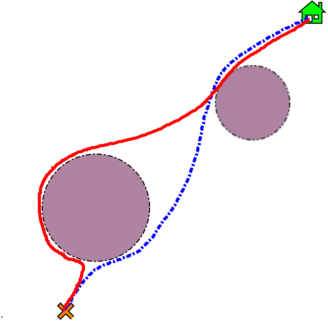
Figure 2: The solid red line and the dashed blue line represent two possible paths on a map. However, sharp turns in the red path typically signal that the vehicle is slowing down at those points, leading to longer travel times and lower solution quality.

$${E_{{{\tilde{z}}_{i}}}} =-(\nabla{P_{att}}({\tilde{z}_{i}}[1:2])+\nabla{P_{rep}}({\tilde{z}_{i}}[1:2]))$$

$$+{E_{v}}({\tilde{z}_{i}}[1:2]),$$

and

$$E_{{{\tilde{z}}_{i}}}^{\dagger}=\frac{{{E_{{{\tilde{z}}_{i}}}}}}{{{{\left\|{{E_{{{\tilde{z}}_{i}}}}}\right\|}_{2}}}}.$$

The introduction of the vortex field also brings other benefits, for instance, it helps to generate smoother trajectories which are less prone to oscillations. The vortex field also reduces the likelihood of local minima traps that generally appear in APF, allowing for more fluid and natural movement through crowded or complex spaces. However, it is worth noting that these paths may be implementable since they may fail to meet the dynamic constraint. In order to overcome this hurdle, we have designed the CVAPF by introducing an extra speed search step. Once the expected moving direction at the current point is determined, the reachable speed towards the expected moving direction will be calculated instantly according to the physical constraints. If achievable speeds exist, the subsequent velocity will then be determined by collaborating the moving direction and a reliable speed. If there exists no speed which meets the constraint combined with the expected moving direction, a safety acceleration will then be applied to slow down the vehicle and divert it toward the expected moving direction simultaneously. The pseudo-code of our proposed CVAPF is demonstrated as Algorithm 2.

Algorithm 2 Customized VAPF Algorithm

1: Input: Map Information $\mathcal{M}$, Current state $z_{0}^{(K)}$. $N\leftarrow 0$; $\tilde{z}_{0}\leftarrow z_{0}^{(K)}$;

2: while ($N<N_{\min}\ \mathtt{or}$ $\ \mathtt{NotSafe}$) do

3:  $\tilde{z}_{N+1}=\tilde{z}_{N}[1:2]+\tilde{z}_{N}[3:4]\cdot\varDelta t$

4:  Calculate $E(\tilde{z}_{N+1}),E^{\dagger}(\tilde{z}_{N+1})$

5:  Search a speed $s_{N+1}$ from $v_{\max}\to 0$ which meets the constraints with the moving direction

6:  if Search is successful then

7:    $\tilde{z}_{N+1}[3:4]=s_{N+1}E^{\dagger}(\tilde{z}_{N+1})$

8:  else

9:   $a_{safe}=[a_{1}E^{\dagger}(\tilde{z}_{N+1})-a_{0}\frac{\tilde{z}_{N}[3:4]}{\|\tilde{z}_{N}[3:4]\|}]$

10:   $\tilde{z}_{N+1}[3:4]=\tilde{z}_{N}[3:4]+a_{safe}\cdot\varDelta t$

11:  end if

12:  Update $\zeta_{v}$

13:  Update $\mathtt{Not\_Safe}$$N\leftarrow N+1$

14: end while

15: if $\mathtt{Not\_Safe}=1$ then

16:  Algorithm Failed;

17: else

18:  Calculate $\{\tilde{u}_{1},\tilde{u}_{2},\cdots\}$

19:  Return Feasible Trajectory $F^{(K)}$

20:  Return $N^{(K)}\leftarrow N$

21: end if

In Algorithm 2, $a_{safe}$ is utilized to lower the speed of the vehicle and alter its direction. Since

$$\begin{gathered}\left\|{{a_{safe}}}\right\|=\left\|{{a_{1}}{E^{\dagger}}({\tilde{z}_{i+1}})-{a_{0}}\frac{{{\tilde{z}_{i}}[3:4]}}{{{\tilde{z}_{i}}[3:4]}}}\right\|,\hfill\\ \leq\left\|{{a_{1}}{E^{\dagger}}({\tilde{z}_{i+1}})}\right\|+\left\|{{a_{0}}\frac{{{\tilde{z}_{i}}[3:4]}}{{{\tilde{z}_{i}}[3:4]}}}\right\|,\hfill\\ ={a_{1}}+{a_{0}},\hfill\\ \end{gathered}$$

$a_{safe}\leq a_{\max}$ can be easily guaranteed by selecting $a_{1}$ and $a_{0}$ with $a_{0}+a_{1}\leq a_{\max}$.

The choice of $N$ also plays a significant role in generating quality trajectories. During our experiments, we have found that it can enhance robustness by having the trajectory searching algorithm terminate at a safer position. For instance, connective infeasibility can greatly be mitigated. This observed phenomenon motivated us to introduce a $\mathtt{Not\_Safe}$ signal accordingly. The update rule for $\mathtt{Not\_Safe}$ can be described as follows:

$$\mathtt{Not\_Safe}=\left\{\begin{gathered}0\ \ \ \hfill({T_{s}}\neq\emptyset)\\ 1\hfill{(else)}\\ \end{gathered}\right.$$

where

$${T_{s}}=\left\{{t\in\left[{0,{t_{w}}}\right]\left|{{z_{N+1}}[1:2]+{z_{N+1}}[3:4]t\in\bigcup\limits_{i=1}^{n_{obs}}{{\mathcal{B}_{i}}}}\right.}\right\}.$$

At the same time, $\min T_{s}$ is a vital parameter used in the updating of $\rho^{(K)}$, where a smaller $\min T_{s}$ requires bigger $\rho^{(K)}$. Since $N^{(K)}$ generated in Algorithm 2 can be large, to maintain the precision, adjusting $N^{(K)}$ is meaningful. These steps also show the necessity to substitute $N^{(K)}$ with $\hat{N}^{(K)}$ in Algorithm 1. Simultaneously, $N_{\max}$ is further introduced to confine the length of applied control input in one planning cycle.

3.4 Customized Dynamic Window Approach (CDWA)

Dynamic Window Approach (DWA) [32] is another kind of seminal algorithm in mobile robotics, which is also renowned for its efficacy in real-time path planning and navigation. By judiciously balancing the trade-offs between speed and safety, DWA enables agents to navigate dynamic environments with minimal risks. The main principle of DWA is exactly the “dynamic window”, which is the set of feasible control inputs an agent can operate at its current states taking into account factors such as position, orientation, speed, and constraints. From the view of the agent, it is critical to predict how it can take action in its current state, which is to construct the dynamic window. From the perspective of the algorithm designer, a policy to decide the action in these sets is paramount to consider.

In order to apply DWA effectively in our scenario, we further develop the CDWA algorithm. Following the general DWA methods, we first identify the dynamical window at the current state, which is achieved by calculating the possible control inputs based on constraints. Next, a subset of these feasible inputs is extracted for evaluation according to the map information, $\mathtt{Not\_Safe}$ flag and $\min T_{s}$. The state of the next time step is instantly anticipated using the chosen input while refreshing the current state by the anticipated state in the end. Repeat these processes several loops to ultimately generate a trajectory consisting of $N$ inputs and $N+1$ states. The pseudo-code of our proposed CDWA is demonstrated in Algorithm 3.

Algorithm 3 Customized DWA Searching Algorithm

1: Input: Map information $\mathcal{M}$, state $z_{0}$.

2: $N\leftarrow 1$;

3: while $N<N_{\min}\ \mathtt{or}$ $\ \mathtt{NotSafe}$ do

4:  Detect Obstacles along the direction of current velocity 

5:  Calculate the dynamic window 

6:  Obtain $\min\{T_{s}\}$ 

7:  Obtain current acceleration 

8:  Update $\mathtt{notsafe}$ 

9:  $N\leftarrow N+1$ 

10: end while

Up to this point, two customized trajectory search algorithms have been provided. We will subsequently show the convergence property of Algorithm 1 in a mild assumption given in Assumption 4.

Assumption 4.

For all planning cycles, there exists $0\leq\kappa<1$, which makes

$$J_{s}({z}^{(K)},{u}^{(K)})\leq\kappa J_{s}(z^{(K-1)},u^{(K-1)})$$ (28)

hold for almost every $K$. In other words, the number of cycles which violate (28) is limited.

To explain the reasonableness of Assumption 4, we can divide the circumstances into two cases. For the case I, consider that $J_{s}^{(K-1)}\gg\gamma$. Under this precondition, the cost from velocity can be set to a relatively small level if a $Q_{0}$ is chosen properly, and the cost function is then mainly decided by the position. Thus, $J_{s}^{(K+1)}\leq J_{s}^{(K)}$ is naturally satisfied with the assistance of the searching algorithm if the initial velocity $z^{(K)}_{0}[3:4]$ is moderate. On the other hand, if the initial velocity is undesirable, e.g. the vehicle moves away from the target area at maximum speed, it can still achieve (28) after several cycles. Furthermore, when the vehicle has to go around an obstacle, decisions need to be made in which direction to turn. Since all the obstacles are circle-like, there exists at least one direction that makes the vehicle get closer to the target area. The search algorithm can prioritize this direction. Experiments also show the mildness of Case I. Case II is complementary to Case I. When $J_{s}^{(K-1)}\gg\gamma$ is not satisfied, properly readjust $\rho^{(K)}$ can drive the vehicle to meet the boundary constraint according to the convexity property of $\mathcal{P}_{s}$ if the trajectory searching algorithm can divert the vehicle to the target area. Thus, Assumption 4 is moderate. Combined with Assumption 1, it can be proven that the target area is reachable within limited planning cycles, as demonstrated in Theorem 1.

Theorem 1.

For given $\gamma$, $z^{(K+1)}_{N+1}$ can be obtained with $\|z^{(K+1)}_{N+1}-z_{f}\|_{Q_{0}}\leq\gamma$ after executing finite planning cycles.

Proof. Under Assumption 4, we only need to suppose (28) is violated at the planning cycle $K_{1},K_{2},\cdots,K_{m}$. Moreover, we define

$$\kappa_{i}=\frac{J_{s}({\lambda_{f}^{(K_{i}+1)}},{\lambda_{d}^{(K_{i}+1)}};\rho^{(K_{i}+1)})}{J_{s}({\lambda_{f}^{(K_{i})}},{\lambda_{d}^{(K_{i})}};\rho^{(K_{i})})}.$$ (29)

We can deduct that $K_{m}+1$ cannot be the last iteration. Then, for any $K\geq K_{m}$, it has

$$\prod\limits_{i=1}^{K}{\frac{{J_{s}({\lambda_{f}^{(i+1)}},{\lambda_{d}^{(i+1)}};\rho^{(i+1)})}}{{J_{s}({\lambda_{f}^{(i)}},{\lambda_{d}^{(i)}};\rho^{(i)})}}}\leq{\kappa^{K-m}}\cdot\prod\limits_{i=1}^{m}{{\kappa_{i}}}.$$ (30)

During each planning cycle but the last one, $\|z^{(K+1)}_{N+1}-z_{f}\|\geq\gamma$ keeps true. As a result, $J_{s}({\lambda_{f}^{(K)}},{\lambda_{d}^{(K)}};\rho^{(K)})\geq\gamma$ are consistently satisfied, which indicates that $\kappa_{i}\leq J_{s}({\lambda_{f}^{(K_{i}+1)}},{\lambda_{d}^{(K_{i}+1)}};\rho^{(K_{i}+1)})/\gamma$ are too bounded for any $\kappa_{i}$. Consequently, we have

$$\left\|{z_{N+1}^{(K+1)}-{z_{f}}}\right\| \leq J_{s}({\lambda_{f}^{(K+1)}},{\lambda_{d}^{(K+1)}},\rho^{(K+1)})$$

$$\leq{\kappa^{K-m}}\cdot\prod\limits_{i=1}^{m}{{\kappa_{i}}}\cdot J_{s}({\lambda_{f}^{(1)}},{\lambda_{d}^{(1)}},\rho^{(1)}).$$ (31)

Take

$$K>\frac{{\left({\log\gamma-\log J_{s}({\lambda_{f}^{(1)}},{\lambda_{d}^{(1)}},\rho^{(1)})-\sum\limits_{i=1}^{m}{\log{\kappa_{i}}}}\right)}}{{\log\kappa}}+m,$$ (32)

we can then guarantee $\|z^{(K+1)}_{N^{(K)}+1}-z_{f}\|_{Q_{0}}\leq\gamma$ after executing $K$ planning cycles, thereby complete the proof. $\square$

Theorem 1 provides conclusive evidence that Algorithm 1 terminates with finite planning cycles under the given assumptions, therefore it is guaranteed that Algorithm 1 generates “practical” trajectories. Building upon this foundation, our subsequent work aims to establish a sufficient condition for the local optimality property of the synthesized trajectory.

Theorem 2.

Suppose $A$, $B$ keeps unchanged during each cycle. Given an initial state $z_{1}$. $\{u_{1},u_{2},\cdots,u_{m}\}$ is an $m$-grids local optimal solution of $\mathcal{P}_{1}^{\prime}(z_{1})$ with $\{z_{1},z_{2},\cdots,z_{m+1}\}$, $\{u^{\prime}_{m^{\prime}+1},\cdots,u_{m+n}\}$ is a local optimal solution of $\mathcal{P}_{1}^{\prime}(z_{m^{\prime}+1})$ at the initial state $z_{m^{\prime}+1}$ with $n$-grids where $1<m^{\prime}\leq m-1$ $(u^{\prime}_{m^{\prime}}$ is applied to distinct with $u_{m^{\prime}}$ in the solution of $\mathcal{P}_{1}^{\prime}(z_{1}))$. Then, $\{u_{1},u_{2},\cdots,u_{m^{\prime}};u^{\prime}_{m^{\prime}+1},\cdots,u_{m^{\prime}+n}\}$ is a local optimal solution of $\mathcal{P}_{1}^{\prime}(z_{1})$ with $m^{\prime}+n$ grids if $u_{m^{\prime}}$ is strictly constrained, i.e. $u_{m^{\prime}}^{\top}Q_{2}u_{m^{\prime}}<1$. Note that $\{u^{\prime}_{m^{\prime}+1},\cdots,u_{m^{\prime}+n}\}$ is extracted from $\mathcal{P}_{1}^{\prime}(z_{m^{\prime}+1})$.

Proof. When $A,B$ are time-invariant in each cycle, suppose $\{z_{1},z_{2},\cdots,z_{m^{\prime}},z_{m^{\prime}+1},\cdots,z_{m^{\prime}+n+1}\}$ is obtained under the synthesized control input. We can formulate the Lagrangian function of $\mathcal{P}_{1}^{\prime}(z_{1})$ with $m^{\prime}+n$ state grids as follows:

$$L_{m^{\prime}+n} =\left\|{{z_{m^{\prime}+n}}}\right\|_{{Q_{0}}}^{2}+\sum\limits_{i=1}^{m^{\prime}+n}{{\upsilon_{i}}\left({{z_{i+1}}-A{z_{i}}-B{u_{i}}-{w_{i}}}\right)}$$

$$+\sum\limits_{i=1}^{m^{\prime}+n+1}{\sum\limits_{j=1}^{{N_{obs}}}{{\zeta_{ij}}\left({r_{j}^{2}-{{\left\|{{z_{i}}[1:2]-{p_{j}}}\right\|}^{2}}}\right)}}$$

$$+\sum\limits_{i=1}^{m^{\prime}+n+1}{{s_{i}}{G_{1}}({z_{i}})}+\sum\limits_{i=1}^{m^{\prime}+n}{{q_{i}}{G_{2}}({u_{i}})}.$$ (33)

Similarly, we can form the Lagrangian function of two separate problems as $L_{m}$ and $L_{n}$. Note that for $i$ with $i\notin\{1,m^{\prime}+1,m^{\prime}+n+1\}$, it could obtain

$$\frac{{\partial{L_{m^{\prime}+n}}}}{{\partial{z_{i}}}}=\frac{\partial}{{\partial{z_{i}}}}\sum\limits_{j=1}^{{N_{obs}}}{{\zeta_{ij}}\left({r_{j}^{2}-{{\left\|{{z_{i}}[1:2]-{p_{j}}}\right\|}^{2}}}\right)}$$

$$-A^{\top}{\upsilon_{i}}+{\upsilon_{i-1}}+2{s_{i}}{Q_{1}}{z_{i}},$$ (34)

and

$$\frac{{\partial{L_{m^{\prime}+n}}}}{{\partial{u_{i}}}}=-{B}^{\top}\upsilon_{i}+2{q_{i}}{Q_{2}}{u_{i}},$$ (35)

which are also the partial derivation of $L_{m}$ or $L_{n}$ respect to $z_{i}$ and $u_{i}$ correspondingly. While for $z_{m^{\prime}+1}$ we have

$$\frac{{\partial{L_{m}}}}{{\partial{z_{m^{\prime}+1}}}} =\frac{\partial}{{\partial{z_{m^{\prime}+1}}}}\sum\limits_{j=1}^{{N_{obs}}}{{\zeta_{m^{\prime}+1,j}}\left({r_{j}^{2}-{{\left\|{{z_{m^{\prime}+1}}[1:2]-{p_{j}}}\right\|}^{2}}}\right)}$$

$$-A^{\top}{\upsilon_{m^{\prime}+1}}+{\upsilon_{m^{\prime}}}+2s_{m^{\prime}+1}{Q_{1}}z_{m^{\prime}+1}.$$

If $u_{m^{\prime}}$ is in the interior of the input constraint, then by the complementary slackness property,

$$\frac{{\partial{L_{m}}}}{{\partial{u_{m^{\prime}}}}}=-{B}^{\top}\upsilon_{m^{\prime}}=\mathbf{0}.$$

Since $B$ is of full column rank, we can obtain that $\upsilon_{m^{\prime}}=\mathbf{0}$. On the other hand, for $L_{n}$, we have

$$\frac{{\partial{L_{n}}}}{{\partial{z_{m^{\prime}+1}}}}={A^{\top}}{\upsilon_{m^{\prime}+1}}+2s_{m^{\prime}+1}{Q_{1}}z_{m^{\prime}+1}$$

$$+\frac{\partial}{{\partial{z_{m^{\prime}+1}}}}\sum\limits_{j=1}^{{N_{obs}}}{2{\zeta_{m^{\prime}+1,j}}{\left({r_{j}^{2}-{{\left\|{{z_{m^{\prime}+1}}[1:2]-{p_{j}}}\right\|}^{2}}}\right)}}.$$ (36)

Although (36) is not required to get zero if we only consider $\mathcal{P}_{1}^{\prime}(z_{m}^{\prime}+1)$, once $L_{m^{\prime}+n}$ reaches optimality, all the variables and multipliers of the synthesized trajectory must lie in the optimal set of $L_{m}$ and $L_{n}$ simultaneously. Thus we have

$$\frac{{\partial{L_{n}}}}{{\partial{z_{m^{\prime}+1}}}}=\frac{{\partial{L_{m}}}}{{\partial{z_{m^{\prime}+1}}}}\Rightarrow{A^{\top}}{\upsilon_{m^{\prime}+1}}={A^{\top}}{\upsilon_{m^{\prime}+1}}+{\upsilon_{m^{\prime}}}.$$ (37)

This equation could be ensured by $\upsilon_{m^{\prime}}=\mathbf{0}$. Note that all other first-order optimality conditions of $L_{m^{\prime}+n}$ can be guaranteed respectively by the KKT condition of $L_{m^{\prime}}$ and $L_{n}$, therefore we can conclude the proof. $\square$

Remark 3.

In Theorem 2, the local optimal property is with respect to $\mathcal{P}_{1}^{\prime}(\cdot)$. Exactly, if (17) is further satisfied in the synthesized solution, it is easy to deduct that the solution is also local optimality in $\mathcal{P}_{1}$.

Analog to the proof of Theorem 2, we can further obtain a stronger conclusion which is demonstrated in Corollary 1.

Corollary 1.

Suppose $A$, $B$ are time-varied matrices between iterations, where we denote them as

$$\{A_{1},\cdots,A_{m^{\prime}},{A^{\prime}}_{m^{\prime}+1},\cdots,A_{m^{\prime}+n}\}$$

and

$$\{B_{1},\cdots,B_{m^{\prime}},{B^{\prime}}_{m^{\prime}+1},\cdots,B_{m^{\prime}+n}\}.$$

Then, Theorem 2 keeps validity under the following two conditions if $m^{\prime}\leq m-2$:

• 1. $u_{m^{\prime}}^{\top}Q_{2}u_{m^{\prime}}<1$ , ${u}_{m^{\prime}+1}^{\top}Q_{2}{u}_{m^{\prime}+1}<1$ and ${u^{\prime}}_{m^{\prime}+1}^{\top}Q_{2}{u^{\prime}}_{m^{\prime}+1}<1$ hold simultaneously;

• 2. $B_{m^{\prime}}$, ${B}_{m^{\prime}+1}$ and ${B^{\prime}}_{m^{\prime}+1}$ are of full column rank.

Theorem 2 and Corollary 1 reveal the reasonableness of synthesis segmented control inputs and further illuminate the rule of adjusting $N^{(K)}$. Although we only considered patching 2 segments in Theorem 2, it is easy to extend the conclusion in multiple trajectory synthesis cases. Moreover, in some specific cases, the aforementioned trajectory synthesizing method can reliably identify the global optimal trajectory, even when dealing with non-convex constraint sets. This result is formally established in Theorem 3.

Theorem 3.

Among the planning cycles, if $\lambda_{\min,i}^{(K)}=0$ keep hold and the condition in Theorem 2 are satisfied, then

$$\{u_{1}^{(1)},\cdots,u_{\hat{N}^{(1)}}^{(1)};u_{1}^{(2)},\cdots,u_{\hat{N}^{(2)}}^{(2)};\cdots;u_{1}^{(K)},\cdots,u_{N^{(K)}}^{(K)}\}$$

in Theorem 2 globally solves $\mathcal{P}_{1}^{\prime}(z_{1})$.

Proof. Let us start by constructing a relaxed problem $\mathcal{P}_{2}^{\prime}(z_{0})$ as

$$\min(z_{N^{(K)}+1}^{(K)}-z_{f})^{\top}Q_{0}(z_{N^{(K)}+1}^{(K)}-z_{f}),$$

$$\mathrm{s.t.\ }\eqref{c2d_var}-\eqref{initial_condition_discrete}.$$

By Theorem 2, $\{z_{1}^{(1)},\cdots,z_{N^{(K)}+1}^{(K)}\}$ is a local optimal trajectory of $\mathcal{P}_{1}^{\prime}(z_{1}^{(1)})$. Note that if all $\lambda_{\min,i}^{(K)}\equiv 0$, the whole trajectories are then unaffected by any of the non-convex obstacles. For the $K$th planning cycle, corresponded solution is optimal of $\mathcal{P}_{w}^{(K)}(\cdot)$, hence we can conclude that $\{z_{1}^{(1)},\cdots,z_{N^{(K)}+1}^{(K)}\}$ is also a local optimal solution of $\mathcal{P}_{2}^{\prime}(z_{1}^{(1)})$. With the convexity of $\mathcal{P}_{2}^{\prime}(\cdot)$, it can further prove the global optimality of $\{z_{1}^{(1)},\cdots,z_{N^{(K)}+1}^{(K)}\}$. Using the fact that the global optimal solution of $\mathcal{P}_{2}^{\prime}(\cdot)$ has a lower or equal cost to the global optimal solution of $\mathcal{P}_{1}^{\prime}(\cdot)$, then it can obtain that $\{z_{1}^{(1)},\cdots,z_{N^{(K)}+1}^{(K)}\}$ is also a global optimal trajectory of $\mathcal{P}_{1}^{\prime(1)}$, which complete the proof. $\square$

The aforementioned theorems have shown the main principle of trajectory synthesizing, establishing that it is possible to find a quality control input for navigating our vehicle by solving optimization problems sequentially and synthesis segment solutions. Furthermore, we have proved that in specific cases, global optimality can be achieved.

In the subsequent discussion, we will delve into another critical index: the travelling time cost. This metric provides insight into how quickly the vehicle can arrive at the target area from its initial state, offering a crucial evaluation of Algorithm 1’s purpose. Generally, various free final time optimization methods can be employed to address time-optimal control problems. Given our discretization is based on fixed step lengths, Algorithm 1 utilizes $\hat{N}^{(K)}$ from its planning cycles to profile time cost. In fact, we can obtain the final time as

$${t_{f}}=h\sum\limits_{i=1}^{K-1}{{{\hat{N}}^{(i)}}}+h{{\hat{N}}^{(K)}}.$$

Since $h{{\hat{N}}^{(K)}}\leq h{N_{\max}}$, one can obtain a preciser evaluation of $t_{f}$ by using a smaller horizon $N_{\max}h$. However, it is unnecessary to calculate an accurate $t_{f}$ to present the “fastness” of the trajectory. Instead, we could demonstrate that $t_{f}$ is achieved approximately to a local minimal final time. To show this claim, suppose that $\{z_{1}^{(j)},\cdots,z_{\hat{N}^{(K)}+1}^{(j)}\}$ are extracted from solving $\mathcal{P}_{1}^{\prime(1)}(z_{0}^{(1)}),\mathcal{P}_{1}^{\prime(2)}(z_{0}^{(2)}),\cdots,\mathcal{P}_{1}^{\prime(K)}(z_{0}^{(K)})$, and the solution of $\mathcal{P}_{1}^{\prime(K)}(z_{0}^{(K)})$ satisfies the quit condition of Algorithm 1, then we have $\hat{N}^{(K)}=N^{(K)}$. If $\{u^{(1)}_{1},\cdots,u^{(K)}_{N^{(K)}+1}\}$ is a local optimal solution of $\mathcal{P}_{1}$, then there exist $\delta$, for arbitrary $\{u^{(1)}_{1}(\delta),\cdots,u^{(K)}_{N^{(K)}+1}(\delta)\}$ which satisfies the constraints with $\|u_{i}^{(j)}-u_{i}^{(j)}(\delta)\|\leq\delta$, we have

$$(z_{N^{(K)}+1}^{(K)}(\delta)-z_{f})^{\top}Q_{0}(z_{N^{(K)}+1}^{(K)}(\delta)-z_{f})\geq\gamma^{2}\geq J^{(K)}.$$

where we denote $z_{(\cdot)}^{(\cdot)}(\delta)$ as the state which obtained by using the control serial $\{u^{(1)}_{1}(\delta),\cdots,u^{(K)}_{N+1}(\delta)\}$. If $(z_{N^{(K)}+1}^{(K)}(\delta)-z_{f})^{\top}Q_{0}(z_{N^{(K)}+1}^{(K)}(\delta)-z_{f})\geq\gamma^{2}$, Algorithm 1 will continue with at least one planning cycle. In this circumstance, suppose $U(\delta)=\{u^{(1)}_{1}(\delta),\cdots,u^{(K)}_{N+1}(\delta),\cdots\}$ is a feasible solution of $\mathcal{P}_{1}$, then it can obtain that

$$t_{f}(\delta)-t_{f}\geq h,$$

where $t_{f}(\delta)$ is the final time of using $U(\delta)$. Otherwise, if $(z_{N^{(K)}+1}^{(K)}(\delta)-z_{f})^{\top}Q_{0}(z_{N^{(K)}+1}^{(K)}(\delta)-z_{f})\leq\gamma^{2}$ then we have $t_{f}(\delta)=t_{f}$. The characteristic of local optimality increases as the time horizon gets smaller. To show this, we rewrite the quit condition to an equivalent form as

$$\|z_{N^{(K)}+1}^{(K)}-z_{f}\|^{2}_{Q_{0}}\leq\gamma^{2}.$$ (38)

Then, we have

$$\|z_{N^{(K)}+1}^{(K)} -z_{f}\|^{2}_{Q_{0}}-\|z_{N^{(K)}+1}^{(K-1)}-z_{f}\|^{2}_{Q_{0}}$$ (39)

$$\leq 2\|z_{1}^{(1)}-z_{f}\|\|z_{N^{(K)}+1}^{(K)}-z_{N^{(K)}+1}^{(K-1)}\|\|Q_{0}\|_{2}$$ (40)

$$\leq 2\|z_{1}^{(1)}-z_{f}\|\cdot(\left\|{z_{{N^{(K)}}+1}^{(K)}-z_{{{\hat{N}}^{(K-1)}}+1}^{(K-1)}}\right\|$$

$$+\left\|{z_{{{\hat{N}}^{(K-1)}}+1}^{(K-1)}-z_{{N^{(K-1)}}+1}^{(K-1)}}\right\|)\cdot\|Q_{0}\|_{2}.$$ (41)

For $\left\|{z_{{N^{(K)}}+1}^{(K)}-z_{{{\hat{N}}^{(K-1)}}+1}^{(K-1)}}\right\|$, we can further obtain

$$\left\|{z_{{N^{(K)}}+1}^{(K)}-z_{{{\hat{N}}^{(K-1)}}+1}^{(K-1)}}\right\|$$

$$=\left\|{z_{{N^{(K)}}+1}^{(K)}-z_{1}^{(K)}}\right\|$$

$$\leq\sum\limits_{i=1}^{N^{(K)}}{\left\|{z_{i+1}^{(K)}-z_{i}^{(K)}}\right\|}$$

$$=h\cdot\sum\limits_{i=1}^{N}{\left\|{{A^{\prime}}z_{i}^{(K)}+{B^{\prime}}u_{i}^{(K)}+{w^{\prime}}_{i}^{(K)}}\right\|}$$

$$\leq N_{\max}h\cdot\mathop{\max}\limits_{i=1,\cdots,N}\left\{{\left\|{{A^{\prime}}z_{i}^{(K)}+{B^{\prime}}u_{i}^{(K)}+{w^{\prime}}_{i}^{(K)}}\right\|}\right\}.$$ (42)

Similarly, we can obtain

$${\left\|{z_{{{\hat{N}}^{(K-1)}}+1}^{(K-1)}-z_{{N^{(K-1)}}+1}^{(K-1)}}\right\|}$$

$$\leq\sum\limits_{i={{\hat{N}}^{(K-1)}}+1}^{{N^{(K-1)}}}{\left\|{z_{i+1}^{(K-1)}-z_{i}^{(K-1)}}\right\|}$$

$$\leq N_{\max}h$$

$$\cdot\max\left\{{\left\|{{A^{\prime}}z_{i}^{(K-1)}+{B^{\prime}}u_{i}^{(K-1)}+{w^{\prime}}_{i}^{(K-1)}}\right\|}\right\}$$ (43)

In the above steps, (40) is a direct result of Assumption 4. With the boundness of $u^{(K)}_{i}$ and $z^{(K)}_{i}$, (41), (42) and (43) indicate $\eqref{time_opt_2}\to 0$ as $N_{\max}h\to 0$. While $\|z_{{N^{(K-1)}}+1}^{(K-1)}-z_{f}\|_{Q_{0}}>\gamma$ and $\|z_{{N^{(K)}}+1}^{(K)}-z_{f}\|_{Q_{0}}\leq\gamma$, we can obtain that $\|z_{{N^{(K)}}+1}^{(K)}-z_{f}\|_{Q_{0}}\to\gamma^{-}$ as $N_{\max}h\to 0$. That means, we can choose a sufficient small $N_{\max}h$, which makes all $\{u^{(1)}_{1}(\delta),\cdots,u^{(K)}_{N+1}(\delta)\}$ failed to meet the quit condition for given $\delta$ except $\{u^{(1)}_{1},\cdots,u^{(K)}_{N+1}\}$ itself. Thus $h\sum\nolimits_{i=1}^{K}{{{\hat{N}}^{(i)}}}$ converges to a local minimal $t_{f}$.

Remark 4.

Although we have $h\sum\nolimits_{i=1}^{K}{{{\hat{N}}^{(i)}}}$ converges to a local minimum as $N_{\max}h\to 0$, some undesired phenomenons may appear if $N_{\max}h$ is too small, e.g. the conditions of Theorem 2 may be difficult to satisfy. Therefore, $t_{f}$ generally approx to a local minimal final time since a lower bound of $N_{\max}h$ should be added.

Next, some sufficient conditions for the equivalence between $\mathcal{P}_{s}(z_{0}^{(K)})$ and $\mathcal{P}_{1}^{\prime}(z_{0}^{(K)})$ will be provided. We begin by defining the relative interior solution.

Definition 2.

For $\mathcal{P}_{s}^{(K)}$, a feasible solution is defined as a relative interior solution if all elements $z_{i}^{(K)}[1:2]$ for $\{i=1,\cdots,N^{(K)}+1\}$ lie within the relative interior of $\mathcal{Z}_{i}[1:2]$.

Theorem 4.

When $\rho^{(K)}=0$, a control serial calculated from the optimal solution of $\mathcal{P}_{s}^{(K)}(z_{0}^{(K)})$ is a local optimal control for $\mathcal{P}_{1}^{\prime}(z_{0}^{(K)})$ if at least one of the following two cases is satisfied:

• All $\lambda_{min,i}^{(K)}=0$ or $\tilde{z}_{i}=\bar{z}_{i}$ for $i\in\{1,\cdots,N^{(K)}+1\}$;

• The obtained optimizer of $\mathcal{P}_{s}^{(K)}$ is a relative interior solution.

Proof. See Appendix A.

Up to this point, we have discussed some properties of Algorithm 1 without the considerations of safety term by setting $\rho^{(j)}=0$ in $\mathcal{P}_{s}^{(j)}(\cdot)$. Next, we will briefly introduce how the safety term affects the solution. Suppose $\{\lambda_{f}^{*}(\rho),\lambda_{d}^{*}(\rho)\}$ is an optimal solution of $\mathcal{P}_{s}(z_{0}^{(K)})$ with $\rho^{(K)}=\rho$. Then we can obtain

$$J(z^{(K)}(\lambda_{f}^{*}(0),\lambda_{d}^{*}(0)),u^{(K)}(\lambda_{f}^{*}(0),\lambda_{d}^{*}(0)))$$

$$+ 0\cdot\|z^{(K)}_{0}-z_{f}\|\|\lambda_{f}^{*}(0)-\mathbf{1}\|^{2}$$

$$\leq J(z^{(K)}(\lambda_{f}^{*}(\rho),\lambda_{d}^{*}(\rho)),u^{(K)}(\lambda_{f}^{*}(\rho),\lambda_{d}^{*}(\rho)))$$

$$+ \rho\cdot\|z^{(K)}_{0}-z_{f}\|\|\lambda_{f}^{*}(\rho)-\mathbf{1}\|^{2}$$

$$\leq J(z^{(K)}(\lambda_{f}^{*}(0),\lambda_{d}^{*}(0)),u^{(K)}(\lambda_{f}^{*}(0),\lambda_{d}^{*}(0)))$$

$$+ \rho\cdot\|z^{(K)}_{0}-z_{f}\|\|\lambda_{f}^{*}(0)-\mathbf{1}\|^{2}$$

$$\leq J(z^{(K)}(\lambda_{f}^{*}(0),\lambda_{d}^{*}(0)),u^{(K)}(\lambda_{f}^{*}(0),\lambda_{d}^{*}(0)))$$

$$+ \rho N_{\max}\|z^{(K)}_{0}-z_{f}\|.$$ (44)

To analyze the trajectory error from the introduction of the safety term, we need to present two important Theorems first, which are demonstrated as Theorem 5 and Theorem 6 respectively.

Theorem 5.

Suppose $f(\mathbf{x})$ is a continuous closed convex function defined in $\mathbf{x}\in\mathbb{E}\subset\mathbb{R}^{l_{f}}$ and the minimum of $f$ is denoted by $f_{opt}$. Define $\Phi_{f}(s)=D_{\mathrm{Lev}(f,s)}$ which is a mapping of $\Phi:[f_{opt},\infty)\to[0,\Phi_{f}(\infty))$, then, $\Phi_{f}(s)$ is upper semi-continuous as $s\in[f_{opt},\infty)$ if $f(\mathbf{x})$ has only one minimizer in $\mathbb{E}$. Where

$$\mathrm{Lev}(f,s)=\left\{{{\bf{x}}:f({\bf{x}})<s}\right\}$$

is the strict level set of $f$ at $s$, and

$$\overline{{\rm{Lev}}}(f,s)=\left\{{{\bf{x}}:f({\bf{x}})\leq s}\right\}$$

is the level set of $f$ at $s$.

Proof. See Appendix B.

Theorem 5 is based on the condition where the optimizer of $f$ is unique. If this condition is not satisfied, it can also easily obtain that $\Phi_{f}(s)$ is upper semi-continuous as $s\in(f_{opt},\infty)$ while its upper semi-continuous range changes to $[\overline{{\rm{Lev}}}(f,f_{opt}),\infty)$. Using similar mathematical method, we can further prove another important theorem, which is presented as Theorem 6.

Theorem 6.

Suppose $X^{*}$ is the optimal set of $f$ with $f(\mathbf{x}^{*})=f_{opt}$ for any $\mathbf{x}^{*}\in X^{*}$. If $X^{*}$ is bounded, Then,

$$\varphi(s)=\left\{\begin{array}[]{l}\mathop{\max}\limits_{{\bf{x}}\in{\rm{Lev(}}f,s{\rm{)}}}\left\{{\left\|{{\rm{Pro}}{{\rm{j}}_{{X^{*}}}}({\bf{x}})-{\bf{x}}}\right\|}\right\}\hfill(s>{f_{opt}})\\ 0\hfill(else)\end{array}\right.$$

is upper semi-continuous as $s\in[f_{opt},\infty)$, and

$$\mathop{\lim}\limits_{s\to f_{opt}^{+}}\left({\mathop{\max}\limits_{{\bf{x}}\in{\rm{cl}}({\rm{Lev}}(f,s))}\left\|{{\bf{x}}-\mathrm{Proj}\left({\bf{x}}\right)}\right\|}\right)=0.$$ (45)

Proof. See Appendix C.

Since $\mathcal{P}_{s}$ is convex, combine (44) we can obtain that as $\rho/\|Q\|_{2}\to 0^{+}$, the difference between $\{\lambda_{f}^{*}(\rho),\lambda_{d}^{*}(\rho)\}$ and $\{\lambda_{f}^{*}(0),\lambda_{d}^{*}(0)\}$ converges to 0 according to the conclusion of Theorem 6. As a result, it is reasonable to consider the solution of $\mathcal{P}_{s}(\cdot)$ as the optimal solution of $\mathcal{P}_{1}^{\prime}(\cdot)$ while ignoring the effect of the safety term, if $\|Q_{0}\|_{2}\gg\rho$ and any of the two cases in Theorem 4 is satisfied.

Despite the aforementioned strict problems can be solved with lower computational burdens, their local optimality condition is not as moderate as initially thought. If a stricter local optimal solution is required, SCP can also be an effective substitution for searching algorithms, That is to use SCP algorithm to get a local optimal solution for each planning cycle. Applying SCP to the two-layer programming model also yields numerous benefits, surpassing the trajectory obtained by directly applying SCP to the original problem. In particular, when both SCP methods have a comparable number of nodes, Algorithm 1 exhibits even greater advantages still due to its reduced computational requirements. This is because Algorithm 1 is only required to calculate a limited set of future trajectory parameters in one cycle, resulting in lower computation power and increased reliability. However, these short-sighted trajectories may arise connective infeasibility while general SCP algorithms do not. Theoretically, the computation complexity and time-optimality of the aforementioned algorithms are drafty tabulated in TABLE I.

Table 1: A Draft Comparison Between Algorithms

	Calculating Time	$t_{f}$
SCP	+++	+
Two-layer model + Searching	+	++
Two-layer model + SCP	++	+

In this table, more “+” represents larger indexes. Although our analysis only guarantees the time optimality for limited scenarios, empirical experiments reveal that the two-layer algorithm excels at generating efficient control inputs with a relatively lower $t_{f}$ and a fast computation speed. More detailed comparisons are given in the next section by numerical experiments.

4 Numerical Experiments

In this section, some numerical experiments are presented to illustrate the capabilities of Algorithm 1 in both static and time-varied map scenarios. We conduct these experiments using MATLAB 2017a with the assistance of the CVX toolbox.

4.1 Experiments with Static Maps

In this part, we generate maps with fixed circular obstacles to evaluate the algorithm’s capability in static scenarios. The critical characteristics of interest can be depicted as vehicle parameters and map parameters, which are presented in Table LABEL:table_parameters.

Table 2: Parameters

Vehicle Parameters	$v_{\max}$	$a_{\max}$	$z_{f}$	$z^{(1)}_{0}$
Range	15	20	$[160,160,0,0]^{\top}$	$0_{4\times 1}$
Map parameters	$n_{obs}$	$r_{i}$	$\ell$	$\gamma$
Range	20	$[3,11]$	7	3

In the process of map generation, The circle obstacles are created and distributed stochastic by built-in random functions, a check step is then used to verify whether the target point is reachable and the map parameters are satisfied. To show the vehicle’s performance to the reader, we randomly choose one map and run simulations respectively with Algorithm 1 and its competition algorithms. The simulated trajectory is visualized in Fig.3.

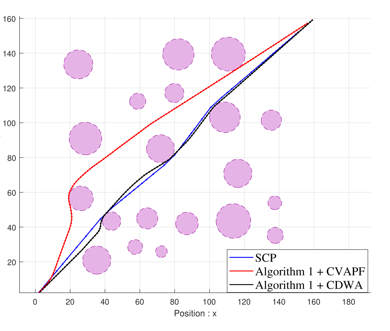
Figure 3: Trajectories generated by 3 distinct algorithm

In Fig.3, The red line represents the trajectory obtained using our two-layer optimization model with the CVAPF searching algorithm, the black line corresponds to the result from Algorithm 1 while utilizing CDWA to get $F^{(K)}$. In contrast, the blue line depicts the trajectory obtained by a general sequential convex programming algorithm, which is parameterized with 45 nodes. Notably, all three trajectories are feasible yet exhibit varying qualities of performance. To facilitate a detailed comparison, we have conducted experiments to measure both the final time and Relative Calculating Time (RCT), as listed in TABLE III.

Table 3: Quality Comparison

	SCP(45 nodes)	SCP(20 nodes)	CVAPF	CDWA
$t_{f}$ (seconds)	24.64	19.3	16.44	15.72
RCT(%)	100*	61.4	34.9	36.9

Correspondingly, the control inputs are shown in Fig.4. In the three charts, the red dashed line represents the acceleration of the $x$-direction, while the blue dashed line represents the acceleration of the $y$-direction.

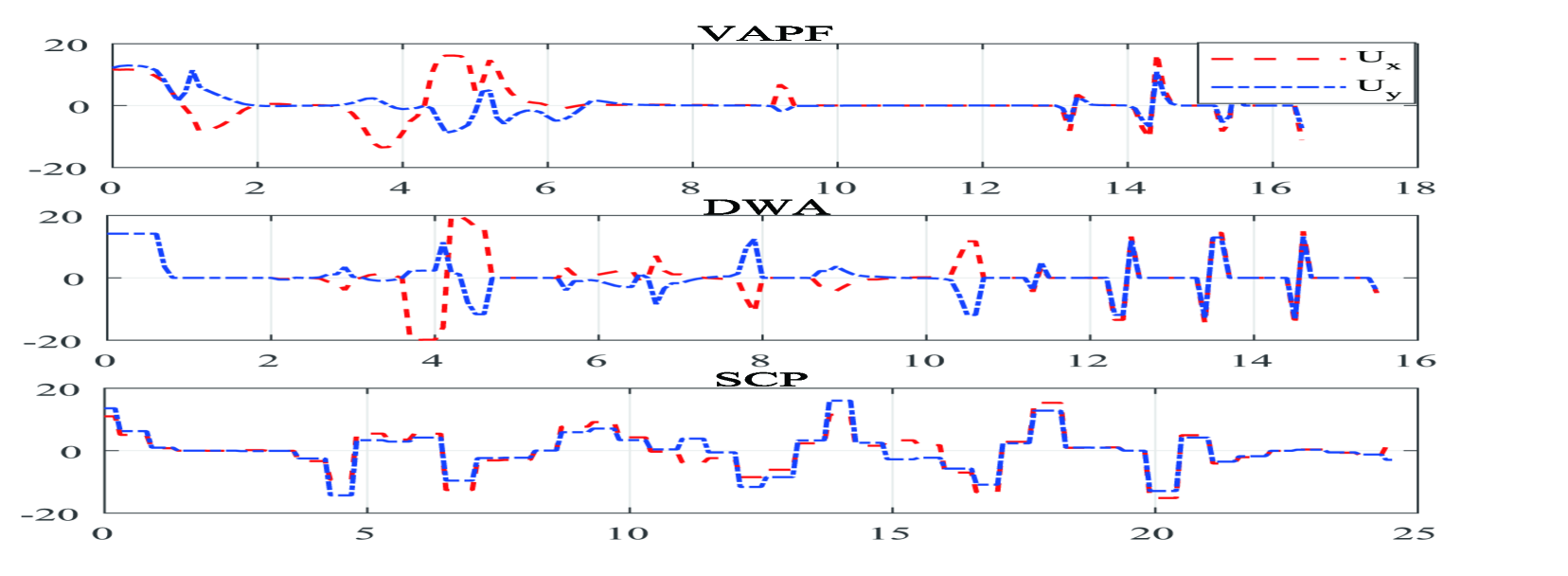
Figure 4: The inputs generated by distinct algorithms: (1) Algorithm 1 with CVAPF, (2) Algorithm 1 with CDWA, and (3) A direct SCP-based approach with 45 nodes.

To further evaluate the capability of Algorithm 1, we employ various metrics in subsequent experiments. Specifically, we utilize indexes such as $t_{f}$, successful rate, and computational time to assess performance. We first test the computation time. In this part, each algorithm is individually tested on 100 maps, with results plotted in Fig. 5 and statistical indicators listed in TABLE IV, where we use SCP45 and SCP20 are the abbreviations of Sequential Convex Programming with 45 Nodes and Sequential Convex Programming with 20 Nodes respectively.

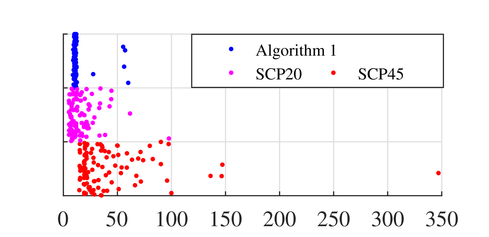
Figure 5: A comparison of the running time between SCPs and our algorithm

Table 4: Quality Comparison of Distinct Algorithms

	SCP45	SCP20	Algorithm 1 + CDWA
Success Rate(%)	90.4	60.2	91.1
RCT(Average)	255.2	100*	74.74
RCT(Worst)	355.2	100*	35.74
RCT(Medium)	220.9	100*	85.11

In TABLE LABEL:tab:tab4, We could further see more details of these experiments which include various metrics for evaluating the performance of our two-layer optimization algorithm, e.g. averaged relative calculating time, worst relative calculating time and the median. Fig.5 further provides insight into the reliability and predictability of our planning model by highlighting the computation time of Algorithm 1 and its competition methods. Notably, it reveals that our two-layer optimization model outperforms SCP algorithms in terms of calculation efficiency, with a shorter average computing time while having a more concentrated distribution of results. In contrast, SCP algorithms exhibit longer computation times and a more scattered distribution, and this is particularly evident as the number of nodes increases. Moreover, it can be observed that each dataset contains significantly larger samples than anticipated. Since our two-layer algorithm requires generating new trajectories before the vehicle reaches the end of its last control sequence, trials with abnormal computation time should be considered as failed experiments and are excluded from successful rate calculations. Despite this limitation, experiment data suggests that Algorithm 1 performs better than a general SCP method in certain static map scenarios.

4.2 Experiments with Dynamic Maps

In this part, we will conduct experiments to show the robustness of Algorithm 1 in time-varied maps with moving obstacles. Firstly, we revise and add some extra parameters shown in Table 5 to profile a time-varied map.

Table 5: The Parameters included in the experiments with time-varying maps

Vehicle Parameters	$v_{\max}$	$a_{\max}$	$z_{f}$	$z^{(1)}_{0}$
Range	6.0	6.0	$[160,160,0,0]^{\top}$	$0_{4\times 1}$
Map parameters	$n$	$r_{i}$	$\epsilon$	$v_{o}$
Range	$\{3,20\}$	$[3,11]$	7	$0.3v_{\max}$

Here, $v_{o}$ is applied to depict the maximal speed of obstacles where for arbitrary $p_{i}(t)$, there exist $\|p_{i}(t+\tilde{t})-p_{i}(t)\|\leq v_{o}\cdot|\tilde{t}|$ for any $t$ and $\tilde{t}$. For demonstration purposes, we initially set the number of obstacles to 3 in a toy example since using a map with fewer obstacles allows for a clear and concise illustration of the algorithm’s behaviour in figures. Then, as part of its validation process, we also test Algorithm 1 with a larger dynamic scenario featuring 20 moved obstacles. To make the motion simulation of the obstacle more realistic, we determine the position of the obstacle by using a double integrator with saturation. In other words, for each simulation step, an obstacle’s velocity is detected at the first. Then, analogue to the DWA, a dynamic acceleration set which meets the subsequent velocity is constructed. The acceleration is randomly selected in these sets instantly. After determining the acceleration, its velocity and position are updated sequentially by numerical integration. In the example, two 3-D figures are plotted to show the specific movement of the vehicle and obstacles in two distinct perspectives, which are demonstrated in Fig. 6.

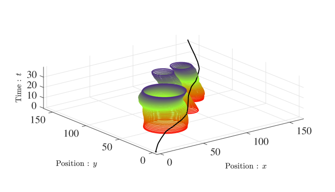
(a)

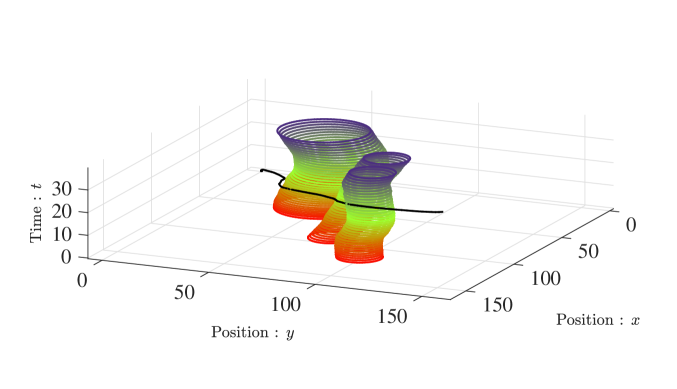
(b)

Figure 6: Obstacle avoidance experiment in time-varied scenarios: A Result

In Fig.6, both graphs share the same vertical axis, representing the time. When the vertical coordinates are specified, the corresponding horizontal plane represents the danger areas from obstacles at that particular moment. The solid black line indicates the vehicle’s trajectory throughout the task. By combining these two charts, it becomes evident that Algorithm 1 effectively avoids obstacles, showcasing its capability with the assistance of searching algorithms in a dynamic map. Furthermore, to aid readers in comprehending the obstacle avoidance capabilities of the vehicle more clearly, we provide a corresponding display diagram as depicted in Fig.7.

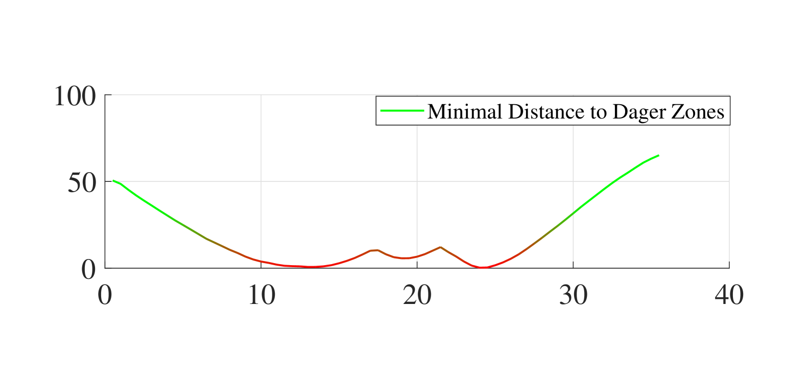
Figure 7: The minimal distance to danger zones during the task. in this figure, the minimal value is 0.2760

In Fig.7, the minimal distance between the vehicle and danger zones is demonstrated. It shows that the vehicle keeps a distance bigger than 0.2760m from all the danger zones at any time.

With $n=20$, we conducted subsequent experiments, testing Algorithm 1 with 150 diverse maps. The results are demonstrated in TABLE 6.

Table 6: Quality Comparison in Time Varying maps

	Successful Rate%	RCT(Average)	RCT(medium)
CVAPF	94.6	93.75	95.71
CDWA	93.3	100*	100*

Next, we will experimentally demonstrate the impact of $v_{\max}$ on the performance of Algorithm 1. In this part, we set $v_{\max}$ as an independent variable and maintain all other parameters constant. To comprehensively evaluate its effects, we tested Algorithm 1 with a large number of randomly created maps, each with distinct $v_{\max}$. The results are presented in TABLE 7.

Table 7: Reliability under Different $v_{\max}$

$v_{\max}$(m/s)	5.0	7.0	9.0	14.0
Successful Rate(%)	87.0	87.5	82.6	76.6

Our previous assertion is supported by this result, which suggests that a smaller $v_{\max}$ tends to yield more flexible steering and improves reliability. In contrast, setting $v_{\max}$ to larger value results in a potential of decreased reliability while the benefit is the reduction of $t_{f}$.

5 Conclusion

Our two-layer optimization-based planning algorithm demonstrated its capability in both theoretical proof and numerical experiments. Specifically, when $v_{\max}$ is well selected, the two-layer planning model outperforms general sequential convex programming algorithms, achieving an optimal balance between time optimality and reliability. However, the model still encounters challenges in extreme scenarios. One key limitation arises from its discrete solution generation, which only guarantees the feasibility in given discrete time points. As a result, it may struggle with feasibility at interpolated states, which is also a common issue faced by general motion planning algorithms. When the planning horizon for a single cycle is excessively long, the timeliness of solutions is compromised, and the algorithm may fail in dynamic scenarios where obstacles continue to shift. Additionally, the computation time for a single planning cycle may exceed the horizon of the latest generated control sequences, potentially leading to loss of vehicle control. To address these shortcomings of Algorithm 1, our future works will focus on enhancing robustness through more reliable searching methods and conducting a detailed analysis of nonlinear vehicle models.

Appendix A Proof of Theorem 4

For simplicity, the indicator of iteration order are omitted, e.g. $z^{(K)}\to z$. Take $\rho=0$. Recall the Lagrange function of $\mathcal{P}_{s}(z_{0})$ can be formulated as $L(z_{0};z,u,\upsilon,\zeta,s,q)$ with the same form of (33). If $L(z_{0};z^{*},u^{*},\upsilon^{*},\zeta^{*},s^{*},q^{*})$ is a local minimum of $L$, then following KKT conditions must be achieved:

$$\left\{\begin{array}[]{l}Az_{i}^{*}+Bu_{i}^{*}-z_{i+1}^{*}={\bf{0}}\\[10.00002pt] s_{i}^{*}{G_{1}}({z_{i}^{*}})={\bf{0}}\\[10.00002pt] q_{i}^{*}{G_{2}}({u_{i}^{*}})={\bf{0}}\\[10.00002pt] \zeta_{ij}^{*}\left({r_{j}^{2}-{{\left\|{{z_{i}^{*}}[1:2]-{p_{j}}}\right\|}^{2}}}\right)={\bf{0}}\\[10.00002pt] s_{i}^{*}\geq 0,q_{i}^{*}\geq 0,\zeta_{ij}^{*}\geq 0\\[10.00002pt] {z_{1}^{*}}={z_{0}}\end{array}\right.$$

and

$$\{{z^{*}_{i}},{u^{*}_{i}}\}=\mathop{\arg\min}\limits_{{z_{i}},{u_{i}}}{L}.$$ (46)

Our goal is to demonstrate that the solution of $\mathcal{P}_{s}(z_{0})$ satisfies the above KKT conditions. Take

$$L^{\prime}=L-\sum\limits_{i=1}^{N+1}{\sum\limits_{j=1}^{{n_{obs}}}{{\zeta_{ij}}\left({r_{j}^{2}-{{\left\|{{z_{i}}[1:2]-{p_{j}}}\right\|}^{2}}}\right)}}.$$

Then, for the strict problem, the following optimal conditions can be derived as

$${L_{s}}(z_{0};z,u,\upsilon,\eta,\sigma,\xi,s,q)=L^{\prime}$$

$$+\sum\limits_{i=1}^{N+1}{({\eta_{i}}-{\sigma_{i}}){\lambda_{f,i}}-{\eta_{i}}}+\sum\limits_{i=1}^{N+1}{{\xi_{i}}({\lambda_{d,i}}-{k_{i}}{\lambda_{f,i}})}.$$ (47)

If $\lambda_{\min,i}=0$ holds for arbitrary $i$, then the nominal trajectory itself is feasible, which is also a minimizer of $L$. Otherwise, if an relative interior solution is obtained, we have

$$\zeta_{ij}^{*}=\eta_{i}^{*}=\sigma_{i}^{*}=\xi_{i}^{*}=0$$

for all $i$ by complement slackness condition. Actually, now we can obtain that $L_{s}\equiv L$. The first order optimality conditions of the strict problem are

$$\left\{\begin{array}[]{l}\frac{{\partial{L_{s}}}}{{\partial{\lambda_{f,i}^{*}}}}=0\\ \\ \frac{{\partial{L_{s}}}}{{\partial{\lambda_{f,d}^{*}}}}=0\end{array}\right.$$ (48)

or

$$\{{\lambda_{f,i}^{*}},{\lambda_{d,i}^{*}}\}=\mathop{\arg\min}\limits_{{\lambda_{f,i}},{\lambda_{d,i}}}{L_{s}}.$$ (49)

In $\mathcal{P}_{s}(\cdot)$, it is worth noting that one pair of $\{\lambda_{f,i},\lambda_{d,i}\}$ determines $\{z_{i}\}$ uniquely. Moreover, since

$$Bu_{i}=z_{i+1}-Az_{i}-w_{i}$$ (50)

and $B$ is of full column rank, we can derive that a given $\{\lambda_{f,i},\lambda_{d,i}\}$ determines a unique state with unique input. In other words, (49) is a sufficient condition of (46), thereby completeing the proof. $\square$

Appendix B Proof of Theorem 5

It is easy to obtain two properties of $\Phi_{f}$: (i). Since the minimizer of $\Phi$ is a singleton, we have $\Phi_{f}(f_{opt})=\Phi_{f}(f_{opt}^{+})=0$; (ii). for $s_{1}\geq s_{2}\geq f_{opt}$, we have $\Phi_{f}(s_{1})\geq\Phi_{f}(s_{2})\geq 0$.

Suppose $\Phi$ is not upper semi-continuous at $\tilde{s}>f_{opt}$. Then, leverage the monotonic non-decrease property of $\Phi_{f}$, for any given $\delta>0$, there exists an $\epsilon>0$ with

$$\Phi_{f}(\tilde{s}+\delta)-\Phi_{f}(\tilde{s})\geq\epsilon.$$ (51)

Suppose $\mathbf{x}(\tilde{s}),\mathbf{y}(\tilde{s})$ are one pair of the cluster points of $\mathrm{Lev}(f,\tilde{s})$ where their distance reaches $D(\mathrm{Lev}(f,\tilde{s}))$. Then, with (51) we can derive that

$$\Phi_{f}(\tilde{s}+\delta)-\Phi_{f}(\tilde{s}) =\|\mathbf{x}(\tilde{s}+\delta)-\mathbf{y}(\tilde{s}+\delta)\|$$

$$-\|\mathbf{x}(\tilde{s})-\mathbf{y}(\tilde{s})\|$$

$$\leq\|\mathbf{x}(\tilde{s}+\delta)-\mathbf{x}(\tilde{s})\|$$

$$+\|\mathbf{y}(\tilde{s}+\delta)-\mathbf{y}(\tilde{s})\|.$$ (52)

Thus, we have

$$\|\mathbf{x}(\tilde{s}+\delta)-\mathbf{x}(\tilde{s})\|+\|\mathbf{y}(\tilde{s}+\delta)-\mathbf{y}(\tilde{s})\|\geq\epsilon.$$ (53)

Since (53) holds for arbitrary $\{\mathbf{x}(\tilde{s}+\delta),\mathbf{y}(\tilde{s}+\delta)\}\subset\mathrm{cl}(D(\mathrm{Lev}(f,\tilde{s}+\delta)))$ with $\|\mathbf{x}(\tilde{s}+\delta)-\mathbf{y}(\tilde{s}+\delta)\|=\Phi_{f}(\tilde{s}+\delta)$, we can further obtain

$$\epsilon \leq\min_{{\bf{x}}(\tilde{s}+\delta),{\bf{y}}(\tilde{s}+\delta)}\left\{{\left\|{{\bf{x}}(\tilde{s}+\delta)-{\bf{x}}(\tilde{s})}\right\|}\right.$$

$$\left.{+\left\|{{\bf{y}}(\tilde{s}+\delta)-{\bf{y}}(\tilde{s})}\right\|}\right\}.$$ (54)

Utilize the fact that all strict level sets are open, we can derive $\mathbf{x}(\tilde{s}),\mathbf{y}(\tilde{s})$ lie on the boundary of $\mathrm{cl}(\mathrm{Lev}(f,\tilde{s}))$ with $f(\mathbf{x}(\tilde{s}))=f(\mathbf{y}(\tilde{s}))=\tilde{s}$. Then, by choosing a non-increasing series $\{\delta_{n}\}$ which converges to 0, we have

$$\left({\mathop{\lim}\limits_{\delta\to{0^{+}}}{\rm{Lev}}(f,\tilde{s}+\delta)}\right)\backslash{\rm{Lev}}(f,\tilde{s})$$

$$=\left({\mathop{\lim}\limits_{n\to\infty}\bigcap\limits_{i=1}^{n}{{\rm{Lev}}(f,\tilde{s}+{\delta_{i}})}}\right)\backslash{\rm{Lev}}(f,\tilde{s}),$$

$$=\overline{{\rm{Lev}}}(f,\tilde{s})\backslash{\rm{Lev}}(f,\tilde{s}),$$

$$=\left\{{{\bf{x}}:f({\bf{x}})=\tilde{s}}\right\}.$$ (55)

By (54), at least one inequality of

$$\left\{\begin{array}[]{l}\left\|{{\bf{x}}(\tilde{s}+\delta)-{\bf{x}}(\tilde{s})}\right\|\geq\varepsilon/2\\ \left\|{{\bf{y}}(\tilde{s}+\delta)-{\bf{y}}(\tilde{s})}\right\|\geq\varepsilon/2\end{array}\right.$$

holds as $\delta\to 0^{+}$, which indicates that at least one of ${{\bf{x}}(\tilde{s}+\delta)}$ or ${{\bf{y}}(\tilde{s}+\delta)}$ is out of $\mathrm{cl}(\mathrm{Lev}(f,\tilde{s}))$ (Note that the fact holds since once ${\bf{x}}(\tilde{s}+\delta),{\bf{y}}(\tilde{s}+\delta)\in\mathrm{cl}(\mathrm{Lev}(f,\tilde{s}))$, (51) and (54) cannot satisfied simultaneously). Hence, suppose $\left\|{{\bf{x}}(\tilde{s}+\delta)-{\bf{x}}(\tilde{s})}\right\|\geq\varepsilon/2$ as $\delta\to 0^{+}$, we can fund a $\mathbf{x}^{\dagger}$ with $\mathbf{x}^{\dagger}\not\in\mathrm{cl}(\mathrm{Lev}(f,\tilde{s})),\mathbf{x}^{\dagger}\in\left({{\rm{Lev}}(f,\tilde{s})\cup\left\{{{\bf{x}}:f({\bf{x}})=\tilde{s}}\right\}}\right)\backslash{\rm{Lev}}(f,\tilde{s})$. Note that

$$\overline{{\rm{Lev}}}(f,\tilde{s})=\left({\mathop{\lim}\limits_{n\to\infty}\bigcap\limits_{i=1}^{n}{{\rm{Lev}}(f,\tilde{s}+{\delta_{i}})}}\right),$$

which preserves the convexity of $\overline{{\rm{Lev}}}(f,\tilde{s})$. Moreover, we have

$$\mathrm{conv}({\rm{Lev}}(f,\tilde{s}),\mathbf{x}^{\dagger})\backslash{\rm{Lev}}(f,\tilde{s})$$

$$\subset\overline{{\rm{Lev}}}(f,\tilde{s})\backslash{\rm{Lev}}(f,\tilde{s}),$$

$$=\left\{{{\bf{x}}:f({\bf{x}})=\tilde{s}}\right\}.$$ (56)

By (56), there exists interior points in $\left\{{{\bf{x}}:f({\bf{x}})=\tilde{s}}\right\}$. Take $\mathbf{x}^{*}\in\mathrm{int}\{\mathbf{x}:f(\mathbf{x})=\tilde{s}\}$ , then there exist $\mathcal{B}(\mathbf{x}^{*},r)$ with $f(\mathbf{x})\equiv\tilde{s}$ for any $\mathbf{x}\in\mathcal{B}(\mathbf{x}^{*},r)$, which indicates $\mathbf{0}\in\partial f(\mathbf{x}^{*})$. By Fermat condition and the convexity of $f$, $\mathbf{x}^{*}$ is an optimizer solution of $f$. However, with $f(\mathbf{x}^{*})=\tilde{s}>f_{opt}$, the optimality of $\mathbf{x}^{*}$ contradicts to the convexity. Hence, $\Phi_{f}$ cannot be discontinuous at $\tilde{s}\in(f_{opt},\infty)$. Combined with (i) we can further derive that $\Phi_{f}(s)$ is upper semi-continuous in $s\in[f_{opt},\infty)$ which completes the proof. $\square$

In the proof, if $f$ is defined in $\mathbb{R}^{l_{f}}$, then $f:\mathbb{E}\to\mathbb{R}$ can also written as $f^{\prime}$:

$$f^{\prime}({\bf{x}})=\left\{\begin{array}[]{l}f({\bf{x}})+{I_{\mathbb{E}}}({\bf{x}})\ \ \hfill({\bf{x}}\in\mathbb{E})\\ {I_{\mathbb{E}}}({\bf{x}})\ \ \hfill({\bf{x}}\notin\mathbb{E}),\end{array}\right.$$

where $I_{\mathbb{E}}$ is the indicator function defined by

$${I_{\mathbb{E}}}({\bf{x}})=\left\{\begin{array}[]{l}0{\rm{}}({\bf{x}}\in\mathbb{E})\\ \infty{\rm{}}({\bf{x}}\notin\mathbb{E}).\end{array}\right.$$

Appendix C Proof of Theorem 6

Suppose there are two non-empty strict level sets $L_{1}=\mathrm{Lev}(f,s_{1})$ and $L_{2}=\mathrm{Lev}(f,s_{2})$, where $\Phi_{f}(s_{1})=D_{1}$, $\Phi_{f}(s_{2})=D_{2}$ and $D_{2}>D_{1}\geq\Phi_{f}(f_{opt}^{+})$. Denote $\mathbf{x}^{*}(D_{1})\in\mathrm{cl}(L_{1}),\mathbf{x}^{*}(D_{2})\in\mathrm{cl}(L_{2})$. $\mathbf{y}^{*}(L_{1}),\mathbf{y}^{*}(L_{2})$ are their projection on $X^{*}$ respectively. Then we have

$$0 \leq\|\mathbf{x}^{*}(L_{2})-\mathbf{y}^{*}(L_{2})\|-\|\mathbf{x}^{*}(L_{1})-\mathbf{y}^{*}(L_{1})\|,$$

$$\leq\|\mathbf{x}^{*}(L_{2})-\mathbf{x}^{*}(L_{1})\|+\|\mathbf{y}^{*}(L_{2})-\mathbf{y}^{*}(L_{1})\|,$$

$$\leq 2\|\mathbf{x}^{*}(L_{2})-\mathbf{x}^{*}(L_{1})\|.$$ (57)

By the boundness of $X^{*}$, $\Phi_{f}(f_{opt}^{+})<\infty$. We first prove (57) converges to 0 as $D_{2}-D_{1}\to 0$. Suppose there exist $\epsilon>0$ which makes $\|\mathbf{x}^{*}(L_{2})-\mathbf{y}^{*}(L_{2})\|-\|\mathbf{x}^{*}(L_{1})-\mathbf{y}^{*}(L_{1})\|\geq\epsilon$ for any $D_{2}>D_{1}>D_{X^{*}}$, then utilize (57) we can obtain

$$\min\left\{{\left\|{{{\bf{x}}^{*}}({L_{2}})-{{\bf{x}}^{*}}({L_{1}})}\right\|}\right\}>\frac{\epsilon}{2},$$

by the continuity of $f$ we can further obtain

$$\min\left\{{\left\|{{{\bf{x}}^{*}}({L_{1}})-{{\bf{x}}^{*}}({L_{1}})}\right\|}\right\}=0>\frac{\epsilon}{2}$$

as $D_{2}\to D_{1}$, which contradicts to $\epsilon>0$. Therefore, we can prove that

$$\max_{\mathbf{x}\in\mathrm{cl}(\mathrm{Lev}(f,s))}\|\mathbf{x}-\mathrm{Proj}_{X^{*}}(\mathbf{x})\|$$ (58)

is an upper semi-continuous mapping of $D$ as $D\in[\Phi_{f}(f_{opt}^{+}),\Phi_{f}(+\infty))$. Moreover, by utilizing (58) we can obtain

$$\varphi(f_{opt})=0=\varphi(f_{opt}^{+}).$$ (59)

References

- [1] B. Paden, M. Čáp, S. Z. Yong, D. Yershov and E. Frazzoli, ”A Survey of Motion Planning and Control Techniques for Self-Driving Urban Vehicles,” in IEEE Transactions on Intelligent Vehicles, vol. 1, no. 1, pp. 33-55, March 2016, doi: 10.1109/TIV.2016.2578706.
- [2] P. E. Hart, N. J. Nilsson and B. Raphael, ”A Formal Basis for the Heuristic Determination of Minimum Cost Paths,” in IEEE Transactions on Systems Science and Cybernetics, vol. 4, no. 2, pp. 100-107, July 1968, doi: 10.1109/TSSC.1968.300136.
- [3] Xiang Liu and Daoxiong Gong, ”A comparative study of A-star algorithms for search and rescue in perfect maze,” 2011 International Conference on Electric Information and Control Engineering, Wuhan, 2011, pp. 24-27, doi: 10.1109/ICEICE.2011.5777723.
- [4] T. Zheng, Y. Xu and D. Zheng, ”AGV Path Planning based on Improved A-star Algorithm,” 2019 IEEE 3rd Advanced Information Management, Communicates, Electronic and Automation Control Conference (IMCEC), Chongqing, China, 2019, pp. 1534-1538, doi: 10.1109/IMCEC46724.2019.8983841.
- [5] G. Tang, C. Tang, C. Claramunt, X. Hu and P. Zhou, ”Geometric A-Star Algorithm: An Improved A-Star Algorithm for AGV Path Planning in a Port Environment,” in IEEE Access, vol. 9, pp. 59196-59210, 2021, doi: 10.1109/ACCESS.2021.3070054.
- [6] Z. Lin, K. Wu, R. Shen, X. Yu and S. Huang, ”An Efficient and Accurate A-Star Algorithm for Autonomous Vehicle Path Planning,” in IEEE Transactions on Vehicular Technology, vol. 73, no. 6, pp. 9003-9008, June 2024, doi: 10.1109/TVT.2023.3348140.
- [7] A. Candra, M. A. Budiman and K. Hartanto, ”Dijkstra’s and A-Star in Finding the Shortest Path: a Tutorial,” 2020 International Conference on Data Science, Artificial Intelligence, and Business Analytics (DATABIA), Medan, Indonesia, 2020, pp. 28-32, doi: 10.1109/DATABIA50434.2020.9190342.
- [8] B. Liu, W. Zhang, W. Chen, H. Huang and S. Guo, ”Online Computation Offloading and Traffic Routing for UAV Swarms in Edge-Cloud Computing,” in IEEE Transactions on Vehicular Technology, vol. 69, no. 8, pp. 8777-8791, Aug. 2020, doi: 10.1109/TVT.2020.2994541.
- [9] A. Stentz, ”Optimal and efficient path planning for partially-known environments,” Proceedings of the 1994 IEEE International Conference on Robotics and Automation, San Diego, CA, USA, 1994, pp. 3310-3317 vol.4, doi: 10.1109/ROBOT.1994.351061.
- [10] Maxim Likhachev, Geoff Gordon, and Sebastian Thrun. 2003. ARA*: anytime A* with provable bounds on sub-optimality. In Proceedings of the 16th International Conference on Neural Information Processing Systems (NIPS’03). MIT Press, Cambridge, MA, USA, 767–774.
- [11] J. J. Kuffner and S. M. LaValle, ”RRT-connect: An efficient approach to single-query path planning,” Proceedings 2000 ICRA. Millennium Conference. IEEE International Conference on Robotics and Automation. Symposia Proceedings (Cat. No.00CH37065), San Francisco, CA, USA, 2000, pp. 995-1001 vol.2, doi: 10.1109/ROBOT.2000.844730.
- [12] Y. Kuwata, J. Teo, G. Fiore, S. Karaman, E. Frazzoli and J. P. How, ”Real-Time Motion Planning With Applications to Autonomous Urban Driving,” in IEEE Transactions on Control Systems Technology, vol. 17, no. 5, pp. 1105-1118, Sept. 2009, doi: 10.1109/TCST.2008.2012116.
- [13] Y. Kuwata, G. A. Fiore, J. Teo, E. Frazzoli and J. P. How, ”Motion planning for urban driving using RRT,” 2008 IEEE/RSJ International Conference on Intelligent Robots and Systems, Nice, France, 2008, pp. 1681-1686, doi: 10.1109/IROS.2008.4651075.
- [14] L. Ma, J. Xue, K. Kawabata, J. Zhu, C. Ma and N. Zheng, ”Efficient Sampling-Based Motion Planning for On-Road Autonomous Driving,” in IEEE Transactions on Intelligent Transportation Systems, vol. 16, no. 4, pp. 1961-1976, Aug. 2015, doi: 10.1109/TITS.2015.2389215.
- [15] S. Karaman, M. R. Walter, A. Perez, E. Frazzoli and S. Teller, ”Anytime Motion Planning using the RRT*,” 2011 IEEE International Conference on Robotics and Automation, Shanghai, China, 2011, pp. 1478-1483, doi: 10.1109/ICRA.2011.5980479.
- [16] A. Perez, R. Platt, G. Konidaris, L. Kaelbling and T. Lozano-Perez, ”LQR-RRT*: Optimal sampling-based motion planning with automatically derived extension heuristics,” 2012 IEEE International Conference on Robotics and Automation, Saint Paul, MN, USA, 2012, pp. 2537-2542, doi: 10.1109/ICRA.2012.6225177.
- [17] R. Mashayekhi, M. Y. I. Idris, M. H. Anisi, I. Ahmedy and I. Ali, ”Informed RRT*-Connect: An Asymptotically Optimal Single-Query Path Planning Method,” in IEEE Access, vol. 8, pp. 19842-19852, 2020, doi: 10.1109/ACCESS.2020.2969316.
- [18] N. Kim, S. Cha and H. Peng, ”Optimal Control of Hybrid Electric Vehicles Based on Pontryagin’s Minimum Principle,” in IEEE Transactions on Control Systems Technology, vol. 19, no. 5, pp. 1279-1287, Sept. 2011, doi: 10.1109/TCST.2010.2061232.
- [19] G. Tang, F. Jiang and J. Li, ”Fuel-Optimal Low-Thrust Trajectory Optimization Using Indirect Method and Successive Convex Programming,” in IEEE Transactions on Aerospace and Electronic Systems, vol. 54, no. 4, pp. 2053-2066, Aug. 2018, doi: 10.1109/TAES.2018.2803558.
- [20] F. Yegenoglu, A. M. Erkmen and H. E. Stephanou, ”Online path planning under uncertainty,” Proceedings of the 27th IEEE Conference on Decision and Control, Austin, TX, USA, 1988, pp. 1075-1079 vol.2, doi: 10.1109/CDC.1988.194483.
- [21] J. Ma, Z. Cheng, X. Zhang, M. Tomizuka and T. H. Lee, ”Alternating Direction Method of Multipliers for Constrained Iterative LQR in Autonomous Driving,” in IEEE Transactions on Intelligent Transportation Systems, vol. 23, no. 12, pp. 23031-23042, Dec. 2022, doi: 10.1109/TITS.2022.3194571.
- [22] D. Malyuta et al., ”Convex Optimization for Trajectory Generation: A Tutorial on Generating Dynamically Feasible Trajectories Reliably and Efficiently,” in IEEE Control Systems Magazine, vol. 42, no. 5, pp. 40-113, Oct. 2022, doi: 10.1109/MCS.2022.3187542.
- [23] B. Açikmeşe and S. R. Ploen, “Convex programming approach to powered descent guidance for mars landing,” AIAA Journal of Guidance, Control and Dynamics, vol. 30, no. 5, pp. 1353–1366, 2007
- [24] J. M. Carson, B. Açikmeşe and L. Blackmore, ”Lossless convexification of Powered-Descent Guidance with non-convex thrust bound and pointing constraints,” Proceedings of the 2011 American Control Conference, San Francisco, CA, USA, 2011, pp. 2651-2656, doi: 10.1109/ACC.2011.5990959.
- [25] B. Açıkmeşe, J. M. Carson and L. Blackmore, ”Lossless Convexification of Nonconvex Control Bound and Pointing Constraints of the Soft Landing Optimal Control Problem,” in IEEE Transactions on Control Systems Technology, vol. 21, no. 6, pp. 2104-2113, Nov. 2013, doi: 10.1109/TCST.2012.2237346.
- [26] O. Khatib, ”Real-time obstacle avoidance for manipulators and mobile robots,” Proceedings. 1985 IEEE International Conference on Robotics and Automation, St. Louis, MO, USA, 1985, pp. 500-505, doi: 10.1109/ROBOT.1985.1087247.
- [27] Y. Gao, D. Li, Z. Sui and Y. Tian, ”Trajectory Planning and Tracking Control of Autonomous Vehicles Based on Improved Artificial Potential Field,” in IEEE Transactions on Vehicular Technology, vol. 73, no. 9, pp. 12468-12483, Sept. 2024, doi: 10.1109/TVT.2024.3389054.
- [28] F. Augugliaro, A. P. Schoellig and R. D’Andrea, ”Generation of collision-free trajectories for a quadrocopter fleet: A sequential convex programming approach,” 2012 IEEE/RSJ International Conference on Intelligent Robots and Systems, Vilamoura-Algarve, Portugal, 2012, pp. 1917-1922, doi: 10.1109/IROS.2012.6385823.
- [29] R. Bonalli, A. Cauligi, A. Bylard and M. Pavone, ”GuSTO: Guaranteed Sequential Trajectory optimization via Sequential Convex Programming,” 2019 International Conference on Robotics and Automation (ICRA), Montreal, QC, Canada, 2019, pp. 6741-6747, doi: 10.1109/ICRA.2019.8794205.
- [30] L. Blackmore, B. Açikmeşe and J. M. Carson, ”Lossless convexification of control constraints for a class of nonlinear optimal control problems,” 2012 American Control Conference (ACC), Montreal, QC, Canada, 2012, pp. 5519-5525, doi: 10.1109/ACC.2012.6314722.
- [31] P. Scheffe, T. M. Henneken, M. Kloock and B. Alrifaee, ”Sequential Convex Programming Methods for Real-Time Optimal Trajectory Planning in Autonomous Vehicle Racing,” in IEEE Transactions on Intelligent Vehicles, vol. 8, no. 1, pp. 661-672, Jan. 2023, doi: 10.1109/TIV.2022.3168130.
- [32] D. Fox, W. Burgard and S. Thrun, ”The dynamic window approach to collision avoidance,” in IEEE Robotics & Automation Magazine, vol. 4, no. 1, pp. 23-33, March 1997, doi: 10.1109/100.580977.