Further Exploration of Precise Binding Energies from Physics Informed Machine Learning and the Development of a Practical Ensemble Model

Abstract

Sixteen new physics informed machine learning models have been trained on binding energy residuals from modern mass models that leverage shape parameters and other physical features. The models have been trained on a subset of AME 2012 data and have been verified with a subset of the AME 2020 data. Among the machine learning approaches tested in this work, the preferred approach is the least squares boosted ensemble of trees which appears to have a superior ability to both interpolate and extrapolate binding energy residuals. The machine learning models for four mass models created from the ensemble of trees approach have been combined to create a composite model called the Four Model Tree Ensemble (FMTE). The FMTE model predicts binding energy values from AME 2020 with a standard deviation of 76 keV and a mean deviation of 34 keV for all nuclei with $N\geq 8$ and $Z\geq 8$. A comparison with new mass measurements for 33 isotopes not included in AME 2012 or AME 2020 indicates that the FMTE performs better than all mass models that were tested.

I Introduction

Accurate predictions of nuclear binding energies are critical for new experimental measurements expanding our understanding of nuclear physics (see e.g., Refs. [1, 2, 3, 4]) and for astrophysical calculations (see e.g., Refs. [5, 6, 7]). Models for binding energies typically reproduce the Atomic Mass Evaluation (AME) experimental values for nuclei with $N\geq 8$ and $Z\geq 8$, with standard deviations, denoted as $\sigma$, ranging from about 200-800 keV [8]. Machine Learning (ML) approaches provide the most accurate fits. These ML approaches have been used to model the binding energy directly using Neural Networks (NNs) [9], or Support Vector Machines (SVM) and Gaussian Process Regression (GPR) [10] which achieve a comparable level of accuracy.

Recently, mass models have been leveraged as a starting point and ML models provide corrections by fitting residuals based on deep NNs [11, 12], convolutional NNs [13], and using tree based ML [14]. Generally, these approaches have been successful in producing good fits to experimental binding energy values.

We have used NNs to fit the residual of binding energies minus a five parameter liquid drop model in Example 1 of Ref. [15]. This resulted in a ML model using only two physical features (the number of protons and the number of neutrons) that was trained on the AME 2012 [16] data that could reproduce the AME 2020 [17] with a standard deviation of $\sigma_{20}=$213 keV using a NN with 300 nodes on both of the two hidden layers used and $\tanh$ as the activation function.

We explored using other ML approaches and more physical features in Ref. [18]. The methodology takes advantage of there being small differences to model when using binding energy residuals, and the approach also takes advantage of the availability of the AME 2012 and AME 2020 datasets. We used the two datasets to ensure that we only trained using trusted values. We then used the values from an independent set of isotopes to determine the best ML model. This step helps to protect against overfitting the data. This resulted in all 12 ML models having values below $\sigma_{20}=$ 240 keV, including the lowest model at $\sigma_{20}=$ 92 keV.

In this manuscript we continue this methodology using SVM [19, 20], GPR [21], Fully Connected Neural Network (FCNN) [15, 22], and the Least Squares Boosted Ensemble of Trees (LSBET) [23, 24] as the ML approaches to model binding energy residuals from four modern mass models.

The four binding energy residuals modeled by each of these four ML approaches result in 16 new models. We leverage the best of these 16 along with the best of 12 prior models from Ref. [18] to develop a composite model that outperforms the other models across all metrics tested.

Section II describes the generation of testing and training sets and the residuals that will be modeled. Section III discusses the four mass models that have been selected. Section IV describes the ML approaches used to generate the new models. Section V describes the physical features that are included in the models. Section VI.1 discusses the intuition that can be gained from calculating the global Shapley value from each model (introduced in [25]). Section VI.2 discusses the creation of a composite model made from four LSBET models. Sections VI.3, VI.4, and VI.5 contain analyses using Garvey-Kelson relationships, model metric comparisons for recent mass measurements, and a test of the extrapolation of the models for neutron rich nuclei, respectively.

II Testing and Training Data

A critical aspect of our approach is the use of robust, independent data sets. We have used the same training and test sets as in Ref. [18]. Specifically, the training set is a subset of AME 2012 [16] that has had 400 isotopes removed. This count results from 57 values that have changed by more than 100 keV, 17 values that were marked as measured in AME 2012 but replaced by extrapolated values in AME 2020, and another 326 values that were one out of every seven values that were reserved for the test set.

There were 121 measurements for new isotopes in AME 2020 that were not included in AME 2012. These 121 measurements, along with the 57 substantially changed values and the 326 random seed values, were combined to create 504 binding energies used in our our test set. Our approach will be to choose the best models based on the performance with the test set.

The mean experimental uncertainties are 20 keV for the training set, 26 keV for the AME 2012, 44 keV for the test set, and 23 keV for the AME 2020 as discussed in Ref. [18]. These values are provided to provide context in the future discussions of the success of different model.

III Mass Models

In the previous work [18], we used two semi-empirical models and the 28-parameter Duflo Zuker (DZ) model from 1995 [26]. The mass models that have been chosen for this analysis are the Finite-Range Droplet Model (FRDM) 2012 [27], Hartree-Fock-Bogoliubov (HFB) 31 [28], Weizsäcker-Skyrme (WS) 4 [29], and WS4+Radial Basis Function (RBF) [29, 30]. The RBF correction used to create the WS4+ values already serves as a residual fit of the data. We have included this model to as a test of how much further improvement is possible within this model.

Each of these mass models are used to create a binding energy residual of the form:

$$\Delta B_{model}=B_{expt.}-B_{model}$$ (1)

The models generated using the WS4+ need to be evaluated carefully because the binding energy residuals are minor corrections, often smaller than 250 keV. The $\Delta B$ values for each of these models has been included in Figure 1a-d.

Figure 1: Binding energy difference, (a) $\Delta B_{FRDM}$, (b) $\Delta B_{HFB}$, (c) $\Delta B_{WS}$, and (d) $\Delta B_{WS4+}$ between the four theoretical models of interest experimental measurements from AME 2020. The 16 new models for $\Delta B$ are (e) FRDMSVM with $C=0.4409$ and $\epsilon=0.0441$, (f) HFBSVM with $C=0.5076$ and $\epsilon=0.0508$, (g) WSSVM with $C=0.2794$ and $\epsilon=0.0279$, (h) WSpSVM with $C=0.1552$ and $\epsilon=0.0155$, (i) FRDMGPR with zero basis function and $\sigma_{f}=0.00344$, (j) HFBGPR with zero basis function and $\sigma_{f}=0.215$, (k) WSGPR with linear basis function and $\sigma_{f}=0.0783$, (l) WSpGPR with linear basis function and $\sigma_{f}=0.0017$, (m) FRDMFCNN with $\lambda=6.25\times 10^{-4}$, (n) HFBFCNN with $\lambda=1.84\times 10^{-3}$, (o) WSFCNN with $\lambda=6.04\times 10^{-4}$, (p) WSpFCNN with $\lambda=3.88\times 10^{-4}$, (q) FRDMLSBET with a minimum leaf size of 20 and $\eta=0.212$, (r) HFBLSBET with a minimum leaf size of 25 and $\eta=0.111$, (s) WSLSBET with a minimum leaf size of 28 and $\eta=0.159$, and (t) WSpLSBET with a minimum leaf size of 31 and $\eta=0.131$.

The models chosen for this analysis have all been published after the AME 2012 was released and these are all models that provide shape parameters that can be used as physical features to also train on. For the FRDM, the deformation parameters $\beta_{2}$, $\beta_{3}$, $\beta_{4}$, and $\beta_{6}$ are determined for the model. For HFB it is the deformation parameters $\beta_{2}$, and $\beta_{4}$, and the charge radius ($R_{C}$), that accompany the binding energy values, and for the WS4 based models the deformation parameters $\beta_{2}$, $\beta_{4}$, and $\beta_{6}$ are provided.

IV Machine Learning Approaches

In total we trained and tested over one thousand machine learning models using the SVM, GPR, FCNN, and LSBET approaches for the four residuals resulting from Eqn. (1). The principles and virtues of each of these approaches has been discussed in Ref. [18]. Here we will focus on just the equations and features that have been optimized.

IV.1 Support Vector Machines

Similar to prior work using SVM regressions (specifically, Ref. [10]), we have also determined that the Gaussian kernel of the form:

$$K_{G}(x_{i},x_{j})=e^{-\gamma r^{2}}$$ (2)

generates the most reliable results. Here $x_{i}$, and $x_{j}$ represent two data points, and $r$ is the Euclidean distance between the two points:

$$r=||x_{i}-x_{j}||=\sqrt{(x_{i}-x_{j})^{T}(x_{i}-x_{j})}$$ (3)

and $\gamma$ is the kernel coefficient.

The optimized hyper-parameters for the SVM models are the kernel scale, box constraint (labeled $C$) which controls the penalty imposed on observations with large residuals, and the $\epsilon$ values that govern the margin of tolerance.

IV.2 Gaussian Process Regression

We have trained GPR models using a variety of kernel function as options. The exponential kernel of the form:

$$K_{exp.}(x_{j},x_{k})=\sigma_{f}^{2}e^{-r/\sigma_{l}}$$ (4)

where $\sigma_{l}$ is the characteristic length scale and $\sigma_{f}$ is the signal noise standard deviation. This kernel was used by the only by the best WSpGPR model.

The Isotropic Matern 5/2 which also involves $r$ from Eqn. (3) which of the form:

$$K_{M5/2}(x_{j},x_{k})=\sigma_{f}^{2}(1+\sqrt{5}r/\sigma_{l}+5r^{2}/{3\sigma_{l}^{2}})e^{-\sqrt{5}r/\sigma_{l}}$$ (5)

is similarly parameterized. It was used by the other three best GPR models. The optimized hyper-parameters for the GPR-based approach are the kernel scale, the type of the basis function used either zero, constant, or linear, and $\sigma_{f}$.

IV.3 Fully Connected Neural Networks

The architecture, parameter definitions, and training procedure for FCNNs were explained in our previous paper [18]. In the present work, the activation function was chosen to be Tanh for all the FCNN models. Variations containing two and three hidden layers were both used. The specific sizes of these layers that we tested are [100, 100], [200, 200], [300, 300], [400, 400], [100, 100, 100], [200, 200, 200], [300, 300, 300], and [400, 400, 400].

For each of these mass models, the networks with two hidden layers performed the best. For the HFB-FCNN model 400 nodes on both layers performed the best. For all other models 200 nodes on each layer performed the best. We have used the $L2$ regularization that consists in adding a penalty term to the loss function to protect against overfitting. The hyperparameter corresponding to this regularization is denoted by $\lambda$.

IV.4 Least Squares Boosted Ensemble of Trees

The LSBET approach, uses multiple decision trees each trained on different subsets of data. It predicts the residual for each tree and then based on the prediction, a step is taken which is scaled by the learning rate (denoted as $\eta$). Lastly, the squared error between the predicted and true values is minimized.

The LSBET models were trained with varying numbers of learners, specifically, 1000, 2000, 3000, 4000, and 5000 learners. The models trained with 3000 learners performed well in two out of the 4 cases. In the remaining two cases, the relative improvement achieved with 5000 learners was negligible. Considering these findings, all the models presented will incorporate 3000 learners.

The optimized hyper-parameters for the LSBET models are the minimum leaf size and the learning rate. The number of leaves indicates the number of data observations that a leaf node must have.

V Physical Features

We have begun with the same 10 physical features as in the previous work [18]. Four of the physical features are directly related to the number of particles in each isotope. These are the proton number ($Z$), neutron number ($N$), mass number ($A=N+Z$) and isospin projection ($T_{Z}=(N-Z)/2$. The next two parameters are the shell scaling parameters from Ref. [31]:

$$\nu=\frac{2N-N_{max}-N_{min}}{N_{max}-N_{min}},$$ (6)

and

$$\zeta=\frac{2Z-Z_{max}-Z_{min}}{Z_{max}-Z_{min}},$$ (7)

where the minimum value of -1 at the beginning of a shell and maximum value of 1 at a closed shell are defined by the nearest magic numbers, and a value of zero occurs if the nucleus is in the middle of a shell. These are based on:

$$N_{min/max}=[2,8,20,28,50,82,126,196],$$ (8)

and

$$Z_{min/max}=[2,8,20,28,50,82,114,124]$$ (9)

that result from Nilsson levels from Ref. [32].

The same Nilsson levels from Ref. [32] are used to define the neutron and proton sub-shell numbers, labeled as $N_{S}$ and $Z_{S}$, that count which sub-shell is occupied by the valence neutrons and protons, starting with 1 for 1s_1/2 orbital, 2 for the 1p_3/2 orbital, 3 for the 1p_1/2 orbital, and so on.

The features $N_{E}$ and $Z_{E}$ are Boolean operators indicating if the neutron or proton number are even (resulting in a value of 1) or odd (resulting in 0).

In addition to these 10 features, each of the mass models used in this analysis have an additional 3 or 4 shape based features that can also be used to train models on.

When including these parameters in pairs there can be up to $2^{7}=128$ possible combinations of pairs of features. We have used in initial Shapley value analysis using all features included to determine a hierarchy of physical features for each model. This has reduced the number of combinations of pairs to about a dozen.

Interestingly, during this preliminary Shapley value analysis it was observed that the ML approach, and not the particular mass model, that consistently dictated which physical features are critical and which are less influential.

VI Results and Discussion

We tested the 13 variations of models where aspects (e.g., $N_{S}$ and $Z_{S}$, or $\nu$ and $\zeta$) of the maximal model were omitted. Table 1 summarizes the seven combinations of physical features that were found to result in a best fit.

Table 1: Physical features used with ML models

Feature	Physical
Group	Features
1	$N,Z,T_{Z},A,\nu,\zeta,N_{E},Z_{E}$, $\beta_{2}$
2	$N,Z,T_{Z},A,\nu,\zeta,N_{S},Z_{S},N_{E},Z_{E}$
3	$N,Z,T_{Z},A,\nu,\zeta,N_{S},Z_{S},N_{E},Z_{E}$, $\beta_{2}$
4	$N,Z,T_{Z},A,\nu,\zeta,41.N_{E},Z_{E}$, $\beta_{2}$, $\beta_{4}$,$R_{C}$
5	$N,Z,T_{Z},A,\nu,\zeta,N_{S},Z_{S},N_{E},Z_{E}$, $\beta_{2}$, $\beta_{4}$, $R_{C}$
6	$N,Z,T_{Z},A,\nu,\zeta,N_{S},Z_{S},N_{E},Z_{E}$, $\beta_{2}$, $\beta_{4}$, $\beta_{6}$
7	$N,Z,T_{Z},A,\nu,\zeta,N_{S},Z_{S},N_{E},Z_{E}$, $\beta_{2}$, $\beta_{3}$, $\beta_{4}$, $\beta_{6}$

Feature Groups 5, 6, and 7 are contain the full listings for their respective models. The features present in each best fit are $N$, $Z$, $T_{Z}$, $A$, $\nu$, $\zeta$, $N_{E}$ and $Z_{E}$. Only Feature Group 2, used by only one model, didn’t take advantage of the shape-based features from the models. It is worth noting that this model and all of the other best fits utilized the shell scaling parameters $\nu$ and $\zeta$, which can serve as a proxy for $\beta_{2}$, because they have one value near a closed shell and another mid-shell. The behavior of $\beta_{2}$ is similar, but generally, it will have a low value if the protons or neutrons are near a closed shell and a higher value if both particles are mid-shell.

Table 2: Best trained models and corresponding evaluation metrics for $\Delta B_{FRDM2012}$, $\Delta B_{HFB31}$, $\Delta B_{WS4}$, and $\Delta B_{WS4+}$ using both AME 2012 [16], and AME 2020 [17] data.

Model	Feature	$\sigma_{12Train}$	$\overline{AE}_{12Train}$	$\sigma_{12}$	$\overline{AE}_{12}$	$\sigma_{20Test}$	$\overline{AE}_{20Test}$	$\sigma_{20}$	$\overline{AE}_{20}$
Name	Group	(MeV)	(MeV)	(MeV)	(MeV)	(MeV)	(MeV)	(MeV)	(MeV)
FRDM2012 [27]		0.571	0.402	0.579	0.410	0.727	0.496	0.606	0.422
FRDMSVM	7	0.235	0.138	0.254	0.150	0.422	0.240	0.284	0.159
FRDMGPR	7	0.067	0.044	0.118	0.063	0.259	0.165	0.133	0.070
FRDMFCNN	3	0.111	0.084	0.153	0.100	0.337	0.189	0.182	0.105
FRDMLSBET	3	0.017	0.013	0.101	0.037	0.266	0.164	0.122	0.046
HFB31 [28]		0.557	0.425	0.570	0.434	0.693	0.514	0.587	0.443
HFBSVM	5	0.322	0.209	0.339	0.221	0.482	0.313	0.360	0.230
HFBGPR	5	0.161	0.113	0.204	0.132	0.404	0.262	0.233	0.144
HFBFCNN	5	0.241	0.177	0.267	0.192	0.441	0.303	0.293	0.203
HFBLSBET	4	0.055	0.042	0.148	0.072	0.378	0.247	0.179	0.085
WS4 [30]		0.286	0.226	0.298	0.233	0.327	0.253	0.295	0.231
WSSVM	6	0.177	0.124	0.196	0.135	0.249	0.178	0.194	0.135
WSGPR	6	0.046	0.032	0.089	0.048	0.185	0.129	0.094	0.053
WSFCNN	6	0.111	0.085	0.150	0.101	0.228	0.161	0.144	0.100
WSLSBET	3	0.021	0.016	0.094	0.038	0.181	0.128	0.085	0.041
WS4+ [30, 29]		0.168	0.131	0.170	0.132	0.253	0.178	0.189	0.141
WSpSVM	6	0.070	0.037	0.082	0.046	0.214	0.133	0.116	0.058
WSpGPR	2	0.000	0.000	0.049	0.014	0.197	0.119	0.090	0.029
WSpFCNN	6	0.085	0.062	0.094	0.067	0.199	0.126	0.118	0.075
WSpLSBET	1	0.023	0.017	0.059	0.031	0.189	0.119	0.088	0.039
FMTE		0.015	0.012	0.081	0.031	0.164	0.112	0.076	0.034

Table 2 contains evaluation metrics for the original models compared to the new ML based models.

Comparisons of the WS with ML models against the original WS4+ model open a window to comparing results from ML approaches against the Radial Basis Function correction. Three of the four ML approaches (WSGPR, WSFCNN, and WSLSBET) outperform the WS4+ model when it comes to the test data and full AME 2020.

The WSpGPR model provides a clear demonstration of model overfitting. The training $\sigma$ and mean absolute error ($\overline{AE}$) values are both on the eV scale with values of 31.2 eV and 23.9 eV, respectively. One might naively believe this to be the best binding energy model, but these values are 6318 and 4965 times larger than the corresponding values using the test set. This case highlights the need for independent test sets. This model is a fit on the level of tens of eV but in practice it extrapolates far less well.

One virtue of the best LSBET models is that they often require fewer physical features than the other ML approaches. Additionally, regarding modeling binding energy residuals they often outperform the other approaches regarding evaluation metrics from the test set. By curating test and training sets, we have taken advantage of the known benefit of random forest approaches, like LSBET, which is that they inherently do not overfit because of the Law of Large Numbers [23].

Figure 1 shows the $\Delta B$ values for each initial model as well as the corresponding ML predicted residual. This demonstrates that for the SVM (Figure 1e-h) and GPR (Figure 1i-l) based models the residuals predicted are localized. Note that the WSGPR and WSpGPR both contain a linear basis function which tilts the background. In the regions further from stability, the FCNN models (Figure 1m-p) occasionally predict residuals that are off-scale compared to the original models (Figure 1a-d). Far from stability, the LSBET models (Figure 1q-t) predict residuals that are comparable to what the known $\Delta B$ values. This further solidifies the case that the LSBET is the preferable approach for modeling binding energy residuals.

VI.1 Understanding the Models Using Shapley Values

Figure 2: Distribution of local Shapley values for the 16 best models listed in order of feature importance for (a) FRDMSVM, (b) HFBSVM, (c) WSSVM, (d) WSpSVM, (e) FRDMGPR, (f) HFBGPR, (g) WSGPR, (h) WSpGPR, (i) FRDMFCNN, (j) HFBFCNN, (k) WSFCNN, (l) WSpFCNN, (m) FRDMLSBET, (n) HFBLSBET, (o) WSLSBET, and (p) WSpLSBET. The vertical spread in points represents how many values are located in the same region. The predictor value color demonstrates if the value for the given input predictor was high or low.

The Shapley values shown in Figure 2 have been sorted in order of overall importance to the model. For example, the $N_{E}$ and $Z_{E}$ values play a highly impactful role (both were in the top 3) for the WS4+ models, shown in the last column of the figure (see subplots d, h, l and p). Whereas, it was either preferable to not include the higher order deformation parameters ($\beta_{4}$ and $\beta_{6}$) or they were among the four least impactful in all of for the WS4+ models.

The features that have a left to right color gradient in Figure 2 are best described as being either monotonically increasing or decreasing. This corresponds to high (and low) values impacting the model consistently in one manner or the other. A good example of this is the dependence on mass number shown in Figure 2g corresponding to the WSGPR model. The high values of $A$ correspond to a negative Shapley value and low values of $A$ correspond to positive Shapley values.

An example of monotonically increasing behavior can be seen in Figure 2j for Z, A, and N, while a monotonically decreasing behavior occurs for $N_{S}$, $Z_{S}$, and $\beta_{2}$ for the HFBFCNN model. In general, color gradients from right to left or left to right shown in Figure 2 are more common among the highest contributing features of the FCNN and LSBET based models where as it is less often present in the SVM and GPR models, indicating that the SVM and GPR models have more complex behavior.

The comparison of the Shapley values for the WS4+ models with all others can provide insights into the potential of using this approach. The impact of WS4+ having already corrected the model with respect to measured masses means that the dominant features $A$, $N$, $Z$, and $T_{Z}$ in each of the SVM models and most of the GPR models seen in the first three columns do not persist in the WS4+ model. In principle, this is because the rudimentary features that in the FRDM, HFB, and WS models have already been accounted for in the Radial Basis Function correction used to create WS+.

The LSBET models (excluding WSpLSBET) are generally not very sensitive to the $N_{E}$ and $Z_{E}$, or $N_{S}$ and $Z_{S}$ values. Instead they depend on a fairly balanced assortment of features. This was also seen previously for the DZLSBET model. Generally, for FRDMLSBET, HFBLSBET, and WSLSBET the $\beta_{2}$ value is of mid-level importance. Overall, there is a complex interplay between the features which are sometimes monotonically increasing or decreasing sometimes not in the LSBET models. It is also worth reiterating that all of the most effective LSBET models exclude features that that would have resulted in a less accurate model.

VI.2 Generation of Composite Mass Model

Figure 3: Binding energy difference $\Delta B$ between the FMTE and AME 2020 [17]. Note that the absolute range displayed here is approximately one sixth of that shown in Figure 1.

This work has resulted in 16 new model which can be added to the 12 models from Ref. [18] to total 28 models that predict masses. Our goal has been to not produce a high number of decent models but instead to generate one superior mass model for external use. Starting with the 28 models generated we have tested millions of combinations of these models and have settled on composite model that is the combination of four LSBET models. The LSBET models were selected because they interpolate well. In Ref. [18], we found that LSBET models also reproduce features that emerge in Garvey-Kelson relations at N=Z whether the original mass model contains that structure or not. Additionally, the LSBET approach consistently results in extrapolated values on scale with what is seen in experiment near stability.

Ensembling models can increase overall accuracy of predictions for several reasons. First, individual models can be weak learners in the entire domain or parts of the domain. The errors made by individual models can be mitigated by ensembling the weak learners especially when the errors are of statistical nature stemming from limited sample size of the training data as we have in our case. Therefore it is not unreasonable to expect that ensembling a set of the best models will, in fact, produce an ensembled model that performs better any of the individual models. While the simplest way to ensemble a regression model is to take the average of their predictions, this might not provide an optimal ensemble. Instead, we have created a weighted average of the best models with the weights chosen that provide the best results for the $\overline{AE}$ for the test set.

The best four models that have been used in the composite model are DZ-LSBET, FRDM-LSBET, HFB-LSBET and WS-LSBET. The mixing ratio that was determined to produce the best MAE in the test set of four LSBET models is: 48.9% WS-LSBET, 42.1% DZ-LSBET, 5.8% FRDM-LSBET, and 3.2% HFB-LSBET. This new model has been termed the Four Model Tree Ensemble (FMTE). It’s worth noting that these ratios can be less precise, meaning that the metrics described in Tables 2 and 3 are unchanged even with modification of these ratios by a percent or two. This weighted average combination of models represents on average a 16% improvement for the 16 metrics shown in Tables 2 and 3 over the alternate of equally using 25% for each of the four models.

Figure 3 contains the $\Delta B$ values for the FMTE model. Further from stability are regions that exceed $|\Delta B|=250\text{keV}$, but the majority of values have $|\Delta B|<50\text{keV}$.

VI.3 Garvey-Kelson Relations

Figure 4: The Garvey-Kelson mass relationships for experimentally measured values, the original models, and the 12 best ML models. (a) experimental values from AME 2020 [17] and (b) FMTE.

The Garvey-Kelson mass relations provide a means of testing the relative output of a binding energy model by comparing nearby values [33]. The two relationships, Eqns. (1) and (3) from Ref. [34], used are:

$$\begin{split}M(N+2,Z-2)-M(N,Z)\\ +M(N,Z-1)-M(N+1,Z-2)\\ +M(N+1,Z)-M(N+2,Z-1)\approx 0,\end{split}$$ (10)

for $N\geq Z$, and

$$\begin{split}M(N-2,Z+2)-M(N,Z)\\ +M(N-1,Z)-M(N-2,Z+1)\\ +M(N,Z+1)-M(N-1,Z+2)\approx 0,\end{split}$$ (11)

for $N<Z$, where $M(N,Z)$ is the mass of an isotope with the corresponding number of protons and neutrons.

Figure 4 demonstrates the values for Garvey-Kelson relations for experimental measurements and for the FMTE model. The FMTE model reproduces the Wigner cusp at $N=Z$ (see, e.g., [35, 36, 37]), where these relations are known to deviate from zero as discussed by Garvey et al. in Ref. [33]. The FMTE model predicts that the phenomena continues for nuclei near the $N=Z$ line. Elsewhere the FMTE model is smooth resulting in Garvey-Kelson relation values that are nearly zero and comparable to what is seen from the experimental values.

VI.4 Comparisons using Recent Mass Measurements

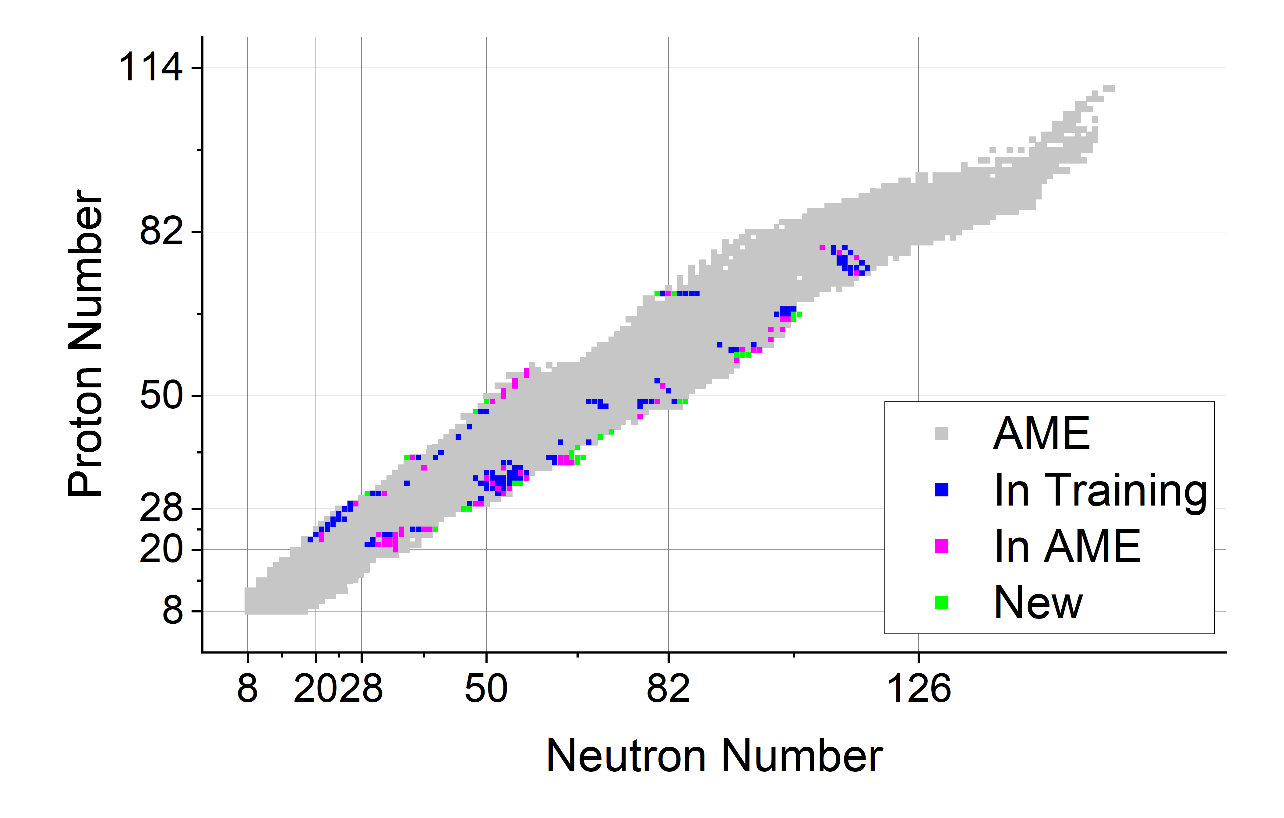
Figure 5: Recent mass measurements grouped by isotopes that were included in the training set, isotopes found in either AME 2012 or AME 2020, and new isotopes not included in either AME set. Isotopes found in either AME 2012 or AME 2020 are indicated in gray.

Table 3: Model evaluation metrics from recent mass measurements from Refs. [38, 39, 40, 41, 42, 43, 44, 45, 46, 47, 48, 49, 50, 51, 52, 53, 54, 55, 56, 57, 58, 59, 60, 61, 62] for five original mass models, the corresponding LSBET models, and the FMTE model.

Model	$\sigma_{Recent}$	$\overline{AE}_{Recent}$	$\sigma_{inTrain}$	$\overline{AE}_{inTrain}$	$\sigma_{inAME}$	$\overline{AE}_{inAME}$	$\sigma_{New}$	$\overline{AE}_{New}$
Name	(MeV)	(MeV)	(MeV)	(MeV)	(MeV)	(MeV)	(MeV)	(MeV)
DZ28 [26]	0.570	0.398	0.411	0.315	0.693	0.486	0.674	0.449
FRDM2012 [27]	0.836	0.631	0.724	0.558	0.945	0.701	0.743	0.549
HFB31 [28]	0.647	0.484	0.578	0.423	0.668	0.497	0.801	0.614
WS4 [30]	0.341	0.267	0.299	0.243	0.318	0.259	0.488	0.360
WS4+ [30, 29]	0.267	0.186	0.196	0.156	0.241	0.178	0.445	0.295
DZLSBET [18]	0.207	0.115	0.058	0.038	0.206	0.157	0.417	0.258
FRDMLSBET	0.246	0.133	0.060	0.040	0.300	0.199	0.420	0.261
HFBLSBET	0.371	0.209	0.077	0.057	0.362	0.281	0.761	0.533
WSLSBET	0.180	0.099	0.060	0.041	0.150	0.117	0.379	0.228
WSpLSBET	0.193	0.102	0.060	0.040	0.186	0.127	0.396	0.253
FMTE	0.175	0.090	0.058	0.038	0.142	0.111	0.376	0.206

A further test of the results from FMTE and the constituate LSBET models was conducted using a survey of recent (i.e., post AME 2020) mass measurements. This survey identified 207 new mass measurements from Refs. [38, 39, 40, 41, 42, 43, 44, 45, 46, 47, 48, 49, 50, 51, 52, 53, 54, 55, 56, 57, 58, 59, 60, 61, 62]. Of these recent measurements, 106 were for isotopes used in the training set. Among these measurements the values changed by 36 keV on average and the average experimental uncertainty is 25 keV. Another 68 measurements were for isotopes included in either AME 2012, AME 2020, or both which have been compared to previously. For these 68 isotopes the average change was 172 keV and 48 keV for these two groups, respectively. The average experimental uncertainty for these 68 measurements was 27 keV. There were an additional 33 measurements for isotopes not included in AME 2012 or AME 2020. The average experimental uncertainty for these newly measured isotopes is 132 keV.

Figure 5 demonstrates the range of isotopes with $N\geq 8$ and $Z\geq 8$ in the AME 2012 and AME 2020. As well as the location of these three subgroups of recent measurements. It is worth noting that many of the previously isotopes that were previously not measured (shown in green in 5) are near the regions where $\Delta B_{FMTE}$ is at it’s highest and lowest extremes, indicating that the model performs less well in that vicinity, nonetheless this is where the new data is.

VI.5 Extrapolation

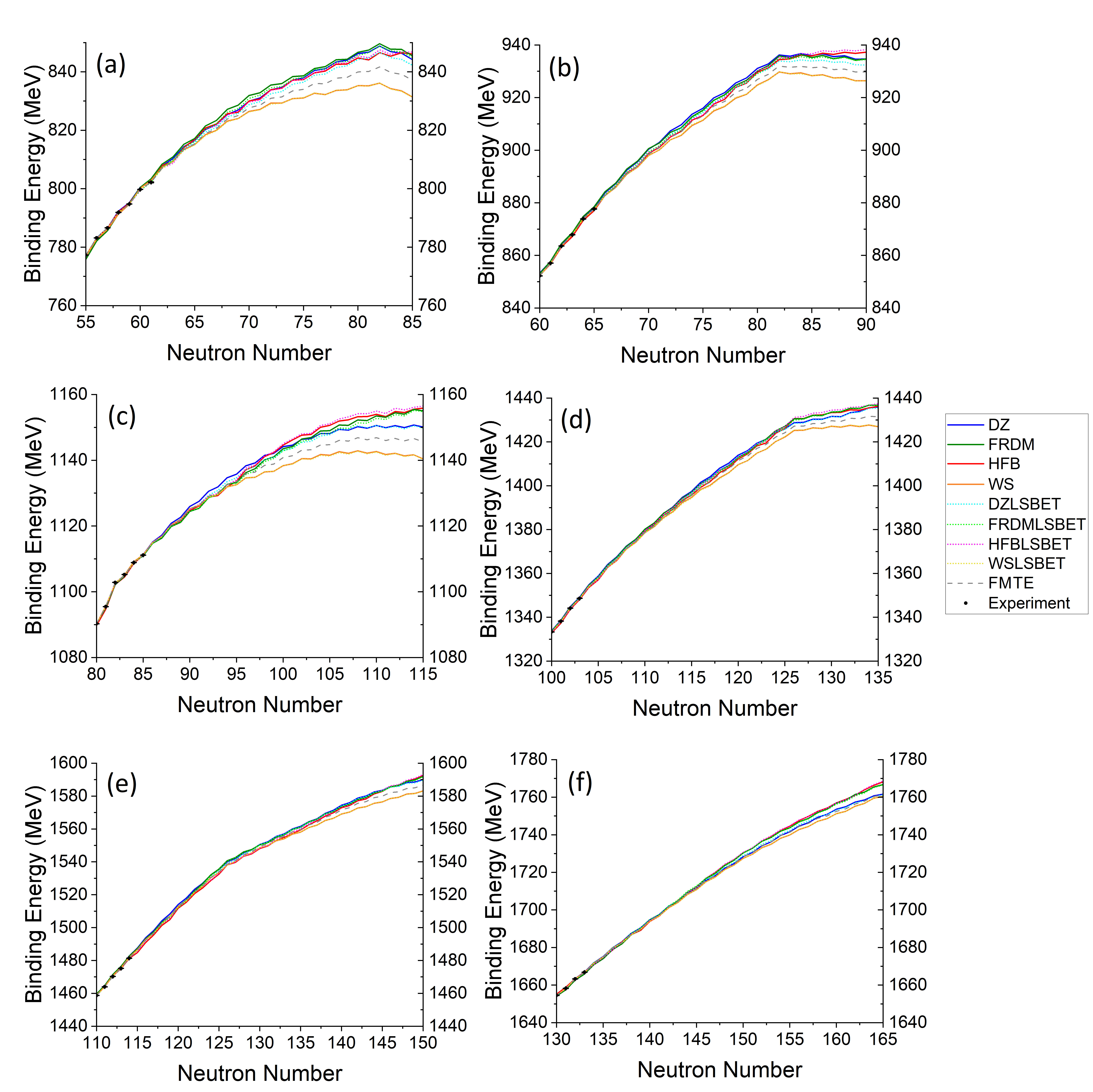
Figure 6: Mass model extrapolation comparison for neutron-rich (a) krypton, (b) zirconium, (c) tin, (d) gadolinium, (e) hafnium, and (f) lead isotopes. Experimental values from AME 2020 [17] are included as black circles. Solid lines indicate the four original models from Refs. [26], [28], [27], and [30]. Dotted lines denote LSBET models including DZLSBET from [18]. The FMTE model is included as the gray dashed lines.

Part of the purpose in producing the FMTE model is to have a model that can be useful for astrophysical calculations. Here we will focus on just the LSBET models and neutron rich nuclei.

Figure 6 shows the four original mass models, the four LSBET based residual models, and the FMTE model created by combining the LSBET models for neutron rich nuclei in six isotopic chains. Figure 6 demonstrates the general characteristic of the LSBET models which is that they generally are correcting each model toward a mid point. The exception to that observation is the HFBLSBET which is a correction that often adds to one of the highest valued models. The FMTE model is the optimized weighted average of the LSBET models as it consists of minor improvements on four of the most commonly used mass models.

VII Summary and Conclusion

We have built on Ref. [18] and further explored using machine learning approaches to model binding energy residuals using contemporary mass models that contain shape features. In 15 of 16 cases the models including some if not all of the shape features outperformed models without those attributes. We followed the previously used methodology including using the same split of training and test data, using Shapley values initially to determine which features might be omitted, and also using Shapley values to better understand the best models by determining if the observed behavior for each feature can be characterized as monotonically increasing or decreasing or more complex.

Generally speaking, our methodology of fitting binding energy residual didn’t improve the WS4+ model as much as other models. This is likely resulting from the fact that this data was already fit to experimental data with the RBF correction. In particular the WSpGPR was a highly precise fit of an already good fit. A comparison between the standard deviations and mean absolute errors of the training and test data sets revealed clear indications of overfitting.

The prior success of DZLSBET and the current success of WSLSBET show that the LSBET technique is the best to use to correct good models that haven’t been previously corrected. In addition to performing well regarding statistical metrics, the LSBET models have extrapolations that are comparable with the original values and result in reasonable Garvey-Kelson relation values (i.e., they reproduce physical features seen in the experimental data). The LSBET models require fewer physical features. If trained on a truly random and representative set then they will not overfit. And lastly, by their nature a group of LSBET models can be ensembled together.

This work culminates in the FMTE model which combines the WSLSBET and DZLSBET, and to a lesser extent the FRDMLSBET and HFBLSBET models. When comparing the various models, the FMTE appears to interpolate and extrapolate better than any other model, as demonstrated in the evaluation metrics involving the test set, the AME 2020 data, and the recent mass measurements. Specifically the $\overline{AE}$ value for the $N\geq 8$ and $Z\geq 8$ isotopes in AME 2020 is 34 keV, which is comparable to the average experimental uncertainty of 23 keV for that set and the corresponding standard deviation value is 76 keV.

The $\overline{AE}=$ 206 keV that the FMTE model has with new masses is roughly 100-400 keV better than the predecessor models though it does fall short of the desired 50 keV target needed for enhanced understanding of astrophysics [63]. Nonetheless, we propose the FMTE for general use including in astrophysical modeling where the constitute models can deviate by 20 MeV.

References

- Ramirez et al. [2012] E. M. Ramirez, D. Ackermann, K. Blaum, M. Block, C. Droese, C. E. Düllmann, M. Dworschak, M. Eibach, S. Eliseev, E. Haettner, F. Herfurth, F. P. Heßberger, S. Hofmann, J. Ketelaer, G. Marx, M. Mazzocco, D. Nesterenko, Y. N. Novikov, W. R. Plaß, D. Rodríguez, C. Scheidenberger, L. Schweikhard, P. G. Thirolf, and C. Weber, Direct mapping of nuclear shell effects in the heaviest elements, Science 337, 1207 (2012), https://www.science.org/doi/pdf/10.1126/science.1225636 .
- Hirsh et al. [2016] T. Y. Hirsh, N. Paul, M. Burkey, A. Aprahamian, F. Buchinger, S. Caldwell, J. A. Clark, A. F. Levand, L. L. Ying, S. T. Marley, G. E. Morgan, A. Nystrom, R. Orford, A. P. Galván, J. Rohrer, G. Savard, K. S. Sharma, and K. Siegl, First operation and mass separation with the caribu mr-tof, Nuclear Instruments and Methods in Physics Research Section B: Beam Interactions with Materials and Atoms 376, 229 (2016), proceedings of the XVIIth International Conference on Electromagnetic Isotope Separators and Related Topics (EMIS2015), Grand Rapids, MI, U.S.A., 11-15 May 2015.
- Vilen et al. [2018] M. Vilen, J. M. Kelly, A. Kankainen, M. Brodeur, A. Aprahamian, L. Canete, T. Eronen, A. Jokinen, T. Kuta, I. D. Moore, M. R. Mumpower, D. A. Nesterenko, H. Penttilä, I. Pohjalainen, W. S. Porter, S. Rinta-Antila, R. Surman, A. Voss, and J. Äystö, Precision mass measurements on neutron-rich rare-earth isotopes at jyfltrap: Reduced neutron pairing and implications for -process calculations, Phys. Rev. Lett. 120, 262701 (2018).
- Wei et al. [2024] J. Wei, C. Alleman, H. Ao, B. Arend, D. Barofsky, S. Beher, G. Bollen, N. Bultman, F. Casagrande, W. Chang, Y. Choi, S. Cogan, P. Cole, C. Compton, M. Cortesi, J. Curtin, K. Davidson, S. D. Carlo, X. Du, K. Elliott, B. Ewert, A. Facco, A. Fila, K. Fukushima, V. Ganni, A. Ganshyn, T. Ginter, T. Glasmacher, A. Gonzalez, Y. Hao, W. Hartung, N. Hasan, M. Hausmann, K. Holland, H. Hseuh, M. Ikegami, D. Jager, S. Jones, N. Joseph, T. Kanemura, S. Kim, C. Knowles, T. Konomi, B. Kortum, N. Kulkarni, E. Kwan, T. Lange, M. Larmann, T. Larter, K. Laturkar, M. LaVere, R. Laxdal, J. LeTourneau, Z.-Y. Li, S. Lidia, G. Machicoane, C. Magsig, P. Manwiller, F. Marti, T. Maruta, E. Metzgar, S. Miller, Y. Momozaki, M. Mugerian, D. Morris, I. Nesterenko, C. Nguyen, P. Ostroumov, M. Patil, A. Plastun, L. Popielarski, M. Portillo, A. Powers, J. Priller, X. Rao, M. Reaume, S. Rodriguez, S. Rogers, K. Saito, B. Sherrill, M. Smith, J. Song, M. Steiner, A. Stolz, O. Tarasov, B. Tousignant, R. Walker, X. Wang, J. Wenstrom, G. West, K. Witgen, M. Wright, T. Xu, Y. Yamazaki, T. Zhang, Q. Zhao, S. Zhao, P. Hurh, S. Prestemon, and T. Shen, Technological developments and accelerator improvements for the frib beam power ramp-up, Journal of Instrumentation 19 (05), T05011.
- Brett et al. [2012] S. Brett, I. Bentley, N. Paul, R. Surman, and A. Aprahamian, Sensitivity of the r-process to nuclear masses, The European Physical Journal A 48, 184 (2012).
- Aprahamian et al. [2014] A. Aprahamian, I. Bentley, M. Mumpower, and R. Surman, Sensitivity studies for the main r process: nuclear masses, AIP Advances 4, 041101 (2014), https://pubs.aip.org/aip/adv/article-pdf/doi/10.1063/1.4867193/12948123/041101_1_online.pdf .
- Martin et al. [2016] D. Martin, A. Arcones, W. Nazarewicz, and E. Olsen, Impact of nuclear mass uncertainties on the process, Phys. Rev. Lett. 116, 121101 (2016).
- Sobiczewski et al. [2018] A. Sobiczewski, Y. Litvinov, and M. Palczewski, Detailed illustration of the accuracy of currently used nuclear-mass models, Atomic Data and Nuclear Data Tables 119, 1 (2018).
- Lovell et al. [2022] A. E. Lovell, A. T. Mohan, T. M. Sprouse, and M. R. Mumpower, Nuclear masses learned from a probabilistic neural network, Phys. Rev. C 106, 014305 (2022).
- Yüksel et al. [2024] E. Yüksel, D. Soydaner, and H. Bahtiyar, Nuclear mass predictions using machine learning models, Phys. Rev. C 109, 064322 (2024).
- Kitouni et al. [2023] O. Kitouni, N. Nolte, S. Trifinopoulos, S. Kantamneni, and M. Williams, Nuclr: Nuclear co-learned representations, arxiv.org 10.48550/arXiv.2306.06099 (2023).
- Choi et al. [2024] S. Choi, K. Kim, Z. He, Y. Kim, and T. Kajino, Deep learning for nuclear masses in deformed relativistic hartree-bogoliubov theory in continuum, arxiv.org 10.48550/arXiv.2411.19470 (2024).
- Lu et al. [2025] Y. Lu, T. Shang, P. Du, J. Li, H. Liang, and Z. Niu, Nuclear mass predictions based on a convolutional neural network, Phys. Rev. C 111, 014325 (2025).
- Liu et al. [2025] G.-P. Liu, H.-L. Wang, Z.-Z. Zhang, and M.-L. Liu, Model-repair capabilities of tree-based machine-learning algorithms applied to theoretical nuclear mass models, Phys. Rev. C 111, 024306 (2025).
- Bentley and Gebran [2025] I. Bentley and M. Gebran, Neural Networks in the Physical Sciences (American Chemical Society, Washington, DC, USA, 2025) https://pubs.acs.org/doi/pdf/10.1021/acsinfocus.7e8014 .
- Wang et al. [2012] M. Wang, G. Audi, A. Wapstra, F. Kondev, M. MacCormick, X. Xu, and B. Pfeiffer, The ame2012 atomic mass evaluation, Chinese Physics C 36, 1603 (2012).
- Wang et al. [2021] M. Wang, W. Huang, F. Kondev, G. Audi, and S. Naimi, The ame 2020 atomic mass evaluation (ii). tables, graphs and references*, Chinese Physics C 45, 030003 (2021).
- Bentley et al. [2025] I. Bentley, J. Tedder, M. Gebran, and A. Paul, High precision binding energies from physics-informed machine learning, Phys. Rev. C 111, 034305 (2025).
- Drucker et al. [1996] H. Drucker, C. J. C. Burges, L. Kaufman, A. Smola, and V. Vapnik, Support vector regression machines, in Advances in Neural Information Processing Systems, Vol. 9, edited by M. Mozer, M. Jordan, and T. Petsche (MIT Press, 1996).
- Janet and Kulik [2020] J. P. Janet and H. J. Kulik, Machine Learning in Chemistry (American Chemical Society, Washington, DC, USA, 2020) https://pubs.acs.org/doi/pdf/10.1021/acs.infocus.7e4001 .
- Rasmussen and Williams [2005] C. Rasmussen and C. Williams, Gaussian Processes for Machine Learning (MIT Press. Cambridge, Massachusetts, 2005).
- Berlyand and Jabin [2023] L. Berlyand and P.-E. Jabin, Mathematics of Deep Learning: An Introduction (De Gruyter, Berlin, Boston, 2023).
- Breiman [2001] L. Breiman, Random forests, Machine Learning 45, 5 (2001).
- Hastie et al. [2009] T. Hastie, R. Tibshirani, and J. Friedman, The Elements of Statistical Learning: Data Mining, Inference, and Prediction, Springer series in statistics (Springer, 2009).
- Shapley [1951] L. S. Shapley, Notes on the n-Person Game-II: The Value of an n-Person Game, Rand Corporation (1951).
- Duflo and Zuker [1995] J. Duflo and A. Zuker, Microscopic mass formulas, Phys. Rev. C 52, R23 (1995).
- Möller et al. [2016] P. Möller, A. Sierk, T. Ichikawa, and H. Sagawa, Nuclear ground-state masses and deformations: Frdm(2012), Atomic Data and Nuclear Data Tables 109-110, 1 (2016).
- Goriely et al. [2016] S. Goriely, N. Chamel, and J. M. Pearson, Further explorations of skyrme-hartree-fock-bogoliubov mass formulas. xvi. inclusion of self-energy effects in pairing, Phys. Rev. C 93, 034337 (2016).
- Wang and Liu [2011] N. Wang and M. Liu, Nuclear mass predictions with a radial basis function approach, Phys. Rev. C 84, 051303 (2011).
- Wang et al. [2014] N. Wang, M. Liu, X. Wu, and J. Meng, Surface diffuseness correction in global mass formula, Physics Letters B 734, 215 (2014).
- Bentley [2016] I. Bentley, Particle-hole symmetry numbers for nuclei, Indian Journal of Physics 90, 1069 (2016).
- Firestone [1999] R. Firestone, Table of Isotopes CD-ROM (Wiley-Interscience, 1999).
- Garvey et al. [1969] G. T. Garvey, W. J. Gerace, R. L. Jaffe, I. Talmi, and I. Kelson, Set of nuclear-mass relations and a resultant mass table, Reviews of modern physics 41, S1 (1969).
- Barea et al. [2008] J. Barea, A. Frank, J. G. Hirsch, P. V. Isacker, S. Pittel, and V. Velázquez, Garvey-kelson relations and the new nuclear mass tables, Physical review. C 77 (2008).
- Satula et al. [1997] W. Satula, D. Dean, J. Gary, S. Mizutori, and W. Nazarewicz, On the origin of the wigner energy, Physics Letters B 407, 103 (1997).
- Jänecke et al. [2002] J. Jänecke, T. W. O’Donnell, and V. I. Goldanskii, Isospin inversion, interactions, and quartet structures in nuclei, Phys. Rev. C 66, 024327 (2002).
- Bentley and Frauendorf [2013] I. Bentley and S. Frauendorf, Relation between wigner energy and proton-neutron pairing, Phys. Rev. C 88, 014322 (2013).
- Silwal et al. [2022] R. Silwal, C. Andreoiu, B. Ashrafkhani, J. Bergmann, T. Brunner, J. Cardona, K. Dietrich, E. Dunling, G. Gwinner, Z. Hockenbery, J. Holt, C. Izzo, A. Jacobs, A. Javaji, B. Kootte, Y. Lan, D. Lunney, E. Lykiardopoulou, T. Miyagi, M. Mougeot, I. Mukul, T. Murböck, W. Porter, M. Reiter, J. Ringuette, J. Dilling, and A. Kwiatkowski, Summit of the n=40 island of inversion: Precision mass measurements and ab initio calculations of neutron-rich chromium isotopes, Physics Letters B 833, 137288 (2022).
- Giraud et al. [2022] S. Giraud, L. Canete, B. Bastin, A. Kankainen, A. Fantina, F. Gulminelli, P. Ascher, T. Eronen, V. Girard-Alcindor, A. Jokinen, A. Khanam, I. Moore, D. Nesterenko, F. de Oliveira Santos, H. Penttilä, C. Petrone, I. Pohjalainen, A. De Roubin, V. Rubchenya, M. Vilen, and J. Äystö, Mass measurements towards doubly magic 78ni: Hydrodynamics versus nuclear mass contribution in core-collapse supernovae, Physics Letters B 833, 137309 (2022).
- Hukkanen et al. [2024] M. Hukkanen, W. Ryssens, P. Ascher, M. Bender, T. Eronen, S. Grévy, A. Kankainen, M. Stryjczyk, O. Beliuskina, Z. Ge, S. Geldhof, M. Gerbaux, W. Gins, A. Husson, D. Nesterenko, A. Raggio, M. Reponen, S. Rinta-Antila, J. Romero, A. de Roubin, V. Virtanen, and A. Zadvornaya, Precision mass measurements in the zirconium region pin down the mass surface across the neutron midshell at N=66, Physics Letters B 856, 138916 (2024).
- Valverde et al. [2024] A. Valverde, F. Kondev, B. Liu, D. Ray, M. Brodeur, D. Burdette, N. Callahan, A. Cannon, J. Clark, D. Hoff, R. Orford, W. Porter, G. Savard, K. Sharma, and L. Varriano, Precise mass measurements of isobars with the canadian penning trap: Resolving the anomaly at 133te, Physics Letters B 858, 139037 (2024).
- Puentes et al. [2020] D. Puentes, G. Bollen, M. Brodeur, M. Eibach, K. Gulyuz, A. Hamaker, C. Izzo, S. M. Lenzi, M. MacCormick, M. Redshaw, R. Ringle, R. Sandler, S. Schwarz, P. Schury, N. A. Smirnova, J. Surbrook, A. A. Valverde, A. C. C. Villari, and I. T. Yandow, High-precision mass measurements of the isomeric and ground states of : Improving constraints on the isobaric multiplet mass equation parameters of the , quintet, Phys. Rev. C 101, 064309 (2020).
- Izzo et al. [2021] C. Izzo, J. Bergmann, K. A. Dietrich, E. Dunling, D. Fusco, A. Jacobs, B. Kootte, G. Kripkó-Koncz, Y. Lan, E. Leistenschneider, E. M. Lykiardopoulou, I. Mukul, S. F. Paul, M. P. Reiter, J. L. Tracy, C. Andreoiu, T. Brunner, T. Dickel, J. Dilling, I. Dillmann, G. Gwinner, D. Lascar, K. G. Leach, W. R. Plaß, C. Scheidenberger, M. E. Wieser, and A. A. Kwiatkowski, Mass measurements of neutron-rich indium isotopes for -process studies, Phys. Rev. C 103, 025811 (2021).
- Mukul et al. [2021] I. Mukul, C. Andreoiu, J. Bergmann, M. Brodeur, T. Brunner, K. A. Dietrich, T. Dickel, I. Dillmann, E. Dunling, D. Fusco, G. Gwinner, C. Izzo, A. Jacobs, B. Kootte, Y. Lan, E. Leistenschneider, E. M. Lykiardopoulou, S. F. Paul, M. P. Reiter, J. L. Tracy, J. Dilling, and A. A. Kwiatkowski, Examining the nuclear mass surface of rb and sr isotopes in the region via precision mass measurements, Phys. Rev. C 103, 044320 (2021).
- Paul et al. [2021] S. F. Paul, J. Bergmann, J. D. Cardona, K. A. Dietrich, E. Dunling, Z. Hockenbery, C. Hornung, C. Izzo, A. Jacobs, A. Javaji, B. Kootte, Y. Lan, E. Leistenschneider, E. M. Lykiardopoulou, I. Mukul, T. Murböck, W. S. Porter, R. Silwal, M. B. Smith, J. Ringuette, T. Brunner, T. Dickel, I. Dillmann, G. Gwinner, M. MacCormick, M. P. Reiter, H. Schatz, N. A. Smirnova, J. Dilling, and A. A. Kwiatkowski, Mass measurements of reduce x-ray burst model uncertainties and extend the evaluated isobaric multiplet mass equation, Phys. Rev. C 104, 065803 (2021).
- Orford et al. [2022] R. Orford, N. Vassh, J. A. Clark, G. C. McLaughlin, M. R. Mumpower, D. Ray, G. Savard, R. Surman, F. Buchinger, D. P. Burdette, M. T. Burkey, D. A. Gorelov, J. W. Klimes, W. S. Porter, K. S. Sharma, A. A. Valverde, L. Varriano, and X. L. Yan, Searching for the origin of the rare-earth peak with precision mass measurements across ce–eu isotopic chains, Phys. Rev. C 105, L052802 (2022).
- Porter et al. [2022] W. S. Porter, E. Dunling, E. Leistenschneider, J. Bergmann, G. Bollen, T. Dickel, K. A. Dietrich, A. Hamaker, Z. Hockenbery, C. Izzo, A. Jacobs, A. Javaji, B. Kootte, Y. Lan, I. Miskun, I. Mukul, T. Murböck, S. F. Paul, W. R. Plaß, D. Puentes, M. Redshaw, M. P. Reiter, R. Ringle, J. Ringuette, R. Sandler, C. Scheidenberger, R. Silwal, R. Simpson, C. S. Sumithrarachchi, A. Teigelhöfer, A. A. Valverde, R. Weil, I. T. Yandow, J. Dilling, and A. A. Kwiatkowski, Investigating nuclear structure near precision mass measurements of neutron-rich ca, ti, and v isotopes, Phys. Rev. C 106, 024312 (2022).
- Xing et al. [2023] Y. M. Xing, C. X. Yuan, M. Wang, Y. H. Zhang, X. H. Zhou, Y. A. Litvinov, K. Blaum, H. S. Xu, T. Bao, R. J. Chen, C. Y. Fu, B. S. Gao, W. W. Ge, J. J. He, W. J. Huang, T. Liao, J. G. Li, H. F. Li, S. Litvinov, S. Naimi, P. Shuai, M. Z. Sun, Q. Wang, X. Xu, F. R. Xu, T. Yamaguchi, X. L. Yan, J. C. Yang, Y. J. Yuan, Q. Zeng, M. Zhang, and X. Zhou, Isochronous mass measurements of neutron-deficient nuclei from projectile fragmentation, Phys. Rev. C 107, 014304 (2023).
- Jaries et al. [2023] A. Jaries, M. Stryjczyk, A. Kankainen, L. Al Ayoubi, O. Beliuskina, P. Delahaye, T. Eronen, M. Flayol, Z. Ge, W. Gins, M. Hukkanen, D. Kahl, S. Kujanpää, D. Kumar, I. D. Moore, M. Mougeot, D. A. Nesterenko, S. Nikas, H. Penttilä, D. Pitman-Weymouth, I. Pohjalainen, A. Raggio, W. Rattanasakuldilok, A. de Roubin, J. Ruotsalainen, and V. Virtanen, High-precision penning-trap mass measurements of cd and in isotopes at jyfltrap remove the fluctuations in the two-neutron separation energies, Phys. Rev. C 108, 064302 (2023).
- Xian et al. [2024] W. Xian, S. Chen, S. Nikas, M. Rosenbusch, M. Wada, H. Ishiyama, D. Hou, S. Iimura, S. Nishimura, P. Schury, A. Takamine, S. Yan, F. Browne, P. Doornenbal, F. Flavigny, Y. Hirayama, Y. Ito, S. Kimura, T. M. Kojima, J. Lee, J. Liu, H. Miyatake, S. Michimasa, J. Y. Moon, S. Naimi, T. Niwase, T. Sonoda, D. Suzuki, Y. X. Watanabe, V. Werner, K. Wimmer, and H. Wollnik, Mass measurements of neutron-rich nuclei constrain element abundances, Phys. Rev. C 109, 035804 (2024).
- Wang et al. [2024] K.-L. Wang, A. Estrade, M. Famiano, H. Schatz, M. Barber, T. Baumann, D. Bazin, K. Bhatt, T. Chapman, J. Dopfer, B. Famiano, S. George, M. Giles, T. Ginter, J. Jenkins, S. Jin, L. Klankowski, S. Liddick, Z. Meisel, N. Nepal, J. Pereira, N. Rijal, A. M. Rogers, O. B. Tarasov, and G. Zimba, Mass measurements of neutron-rich nuclei near , Phys. Rev. C 109, 035806 (2024).
- Jaries et al. [2024] A. Jaries, S. Nikas, A. Kankainen, T. Eronen, O. Beliuskina, T. Dickel, M. Flayol, Z. Ge, M. Hukkanen, M. Mougeot, I. Pohjalainen, A. Raggio, M. Reponen, J. Ruotsalainen, M. Stryjczyk, and V. Virtanen, Probing the midshell region for the process via precision mass spectrometry of neutron-rich rare-earth isotopes with the jyfltrap double penning trap, Phys. Rev. C 110, 045809 (2024).
- Kimura et al. [2024] S. Kimura, M. Wada, H. Haba, H. Ishiyama, S. Ishizawa, Y. Ito, T. Niwase, M. Rosenbusch, P. Schury, and A. Takamine, Comprehensive mass measurement study of fission fragments with mrtof-ms and detailed study of masses of neutron-rich ce isotopes, Phys. Rev. C 110, 045810 (2024).
- Ireland et al. [2025] C. M. Ireland, F. M. Maier, G. Bollen, S. E. Campbell, X. Chen, H. Erington, N. D. Gamage, M. J. Gutiérrez, C. Izzo, E. Leistenschneider, E. M. Lykiardopoulou, R. Orford, W. S. Porter, D. Puentes, M. Redshaw, R. Ringle, S. Rogers, S. Schwarz, L. Stackable, C. S. Sumithrarachchi, A. A. Valverde, A. C. C. Villari, and I. T. Yandow, High-precision mass measurement of restores smoothness of the mass surface, Phys. Rev. C 111, 014314 (2025).
- Mukai et al. [2025] M. Mukai, Y. Hirayama, P. Schury, Y. X. Watanabe, T. Hashimoto, N. Hinohara, S. C. Jeong, H. Miyatake, J. Y. Moon, T. Niwase, M. Reponen, M. Rosenbusch, H. Ueno, and M. Wada, Evidence for shape transitions near through direct mass measurements, Phys. Rev. C 111, 014322 (2025).
- Wolfgruber et al. [2024] T. Wolfgruber, M. Knöll, and R. Roth, Precise neural network predictions of energies and radii from the no-core shell model, Phys. Rev. C 110, 014327 (2024).
- Leistenschneider et al. [2021] E. Leistenschneider, E. Dunling, G. Bollen, B. A. Brown, J. Dilling, A. Hamaker, J. D. Holt, A. Jacobs, A. A. Kwiatkowski, T. Miyagi, W. S. Porter, D. Puentes, M. Redshaw, M. P. Reiter, R. Ringle, R. Sandler, C. S. Sumithrarachchi, A. A. Valverde, and I. T. Yandow (The LEBIT Collaboration and the TITAN Collaboration), Precision mass measurements of neutron-rich scandium isotopes refine the evolution of and shell closures, Phys. Rev. Lett. 126, 042501 (2021).
- Beck et al. [2021] S. Beck, B. Kootte, I. Dedes, T. Dickel, A. A. Kwiatkowski, E. M. Lykiardopoulou, W. R. Plaß, M. P. Reiter, C. Andreoiu, J. Bergmann, T. Brunner, D. Curien, J. Dilling, J. Dudek, E. Dunling, J. Flowerdew, A. Gaamouci, L. Graham, G. Gwinner, A. Jacobs, R. Klawitter, Y. Lan, E. Leistenschneider, N. Minkov, V. Monier, I. Mukul, S. F. Paul, C. Scheidenberger, R. I. Thompson, J. L. Tracy, M. Vansteenkiste, H.-L. Wang, M. E. Wieser, C. Will, and J. Yang, Mass measurements of neutron-deficient yb isotopes and nuclear structure at the extreme proton-rich side of the shell, Phys. Rev. Lett. 127, 112501 (2021).
- Li et al. [2022] H. F. Li, S. Naimi, T. M. Sprouse, M. R. Mumpower, Y. Abe, Y. Yamaguchi, D. Nagae, F. Suzaki, M. Wakasugi, H. Arakawa, W. B. Dou, D. Hamakawa, S. Hosoi, Y. Inada, D. Kajiki, T. Kobayashi, M. Sakaue, Y. Yokoda, T. Yamaguchi, R. Kagesawa, D. Kamioka, T. Moriguchi, M. Mukai, A. Ozawa, S. Ota, N. Kitamura, S. Masuoka, S. Michimasa, H. Baba, N. Fukuda, Y. Shimizu, H. Suzuki, H. Takeda, D. S. Ahn, M. Wang, C. Y. Fu, Q. Wang, S. Suzuki, Z. Ge, Y. A. Litvinov, G. Lorusso, P. M. Walker, Z. Podolyak, and T. Uesaka, First application of mass measurements with the rare-ri ring reveals the solar -process abundance trend at and , Phys. Rev. Lett. 128, 152701 (2022).
- Ge et al. [2024] Z. Ge, M. Reponen, T. Eronen, B. Hu, M. Kortelainen, A. Kankainen, I. Moore, D. Nesterenko, C. Yuan, O. Beliuskina, L. Cañete, R. de Groote, C. Delafosse, T. Dickel, A. de Roubin, S. Geldhof, W. Gins, J. D. Holt, M. Hukkanen, A. Jaries, A. Jokinen, A. Koszorús, G. Kripkó-Koncz, S. Kujanpää, Y. H. Lam, S. Nikas, A. Ortiz-Cortes, H. Penttilä, D. Pitman-Weymouth, W. Plaß, I. Pohjalainen, A. Raggio, S. Rinta-Antila, J. Romero, M. Stryjczyk, M. Vilen, V. Virtanen, and A. Zadvornaya, High-Precision Mass Measurements of Neutron Deficient Silver Isotopes Probe the Robustness of the Shell Closure, Phys. Rev. Lett. 133, 132503 (2024).
- M. Zhang et al. [2023] M. Zhang et al., -defined isochronous mass spectrometry and mass measurements of fragments, Eur. Phys. J. A 59, https://doi.org/10.1140/epja/s10050-023-00928-6 (2023).
- M. Mougeot et al. [2021] M. Mougeot et al., Mass measurements of 99–101in challenge ab initio nuclear theory of the nuclide 100sn, Nature Physics 17, https://doi.org/10.1038/s41567-021-01326-9 (2021).
- Clark et al. [2023] J. Clark, G. Savard, M. Mumpower, and A. Kankainen, Precise mass measurements of radioactive nuclides for astrophysics, Eur. Phys. J. A 59, 10.1140/epja/s10050-023-01037-0 (2023).