Magnetoconductivity due to electron-electron interaction
in a non-Galilean–invariant Fermi liquid

Abstract

The $T^{2}$-scaling of resistivity with temperature is often viewed as a classic hallmark of a Fermi-liquid (FL) behavior in metals. However, if umklapp scattering is suppressed, this scaling is not universally guaranteed to occur. In this case, the resistivity behavior is influenced by several factors, such as dimensionality (two vs. three), topology (simply- vs. multiply-connected Fermi surfaces), and (in two dimensions) the shape (convex vs. concave) of the Fermi surface (FS). Specifically for an isotropic spectrum, as well as for a two-dimensional (2D) convex FS, the $T^{2}$ term is absent, and the first non-zero contribution scales as $T^{4}\ln T$ in 2D and as $T^{4}$ in 3D. In this paper, we study the $T$-dependence of the resistivity, arising from electron-electron interactions, in the presence of a weak magnetic field. We show that, for an isotropic FS in any dimensions and for a convex 2D FS, the $T^{2}$ term is also absent in both Hall and diagonal magnetoconductivity, which instead scale as $BT^{4}\ln T$ and $B^{2}T^{4}\ln T$, respectively, in 2D and as $BT^{4}$ and $B^{2}T^{4}$ in 3D. The FL-like scaling, i.e., $BT^{2}$ and $B^{2}T^{2}$ of the Hall and diagonal conductivities is recovered for a concave FS in 2D. Furthermore, we show that, for an isotropic spectrum, magnetoresistance is absent even in the presence of electron-electron interactions. Additionally, we examine the high-temperature limit, when electron-electron scattering prevails over electron-impurity one, and show that all components of the conductivity tensor saturate in this limit at values that are determined by impurity scattering but, in general, differ from the corresponding values at $T=0$.

I Introduction

It is well established that electron-electron (ee) interactions can influence the resistivity of a non-Galilean invariant Fermi-liquid (FL) metal. The $T^{2}$ scaling of resistivity, which is regarded as a characteristic feature of FL behavior in metals, can be understood through the Pauli exclusion principle. This principle indicates that at low temperatures, only quasiparticles near the Fermi energy, within a width on the order of $T$, participate in binary collisions. It is important to note, however, that this argument pertains to the inverse quasiparticle relaxation time $1/\tau_{\mathrm{ee}}$ rather than the resistivity itself. For example, a Galilean-invariant FL has zero resistivity but finite thermal conductivity and viscosity, whose temperature dependences follow from the $T^{2}$ scaling of $1/\tau_{\mathrm{ee}}$. This is because in a Galilean-invariant system velocities are proportional to momenta, and conservation of momentum automatically implies conservation of the electric current. Hence, a momentum relaxation mechanism is needed in order to achieve a steady-state current.

In metals, the presence of a lattice breaks Galilean invariance, allowing for current relaxation through umklapp scattering [1], which conserves quasi-momentum up to a reciprocal lattice vector. For umklapp scattering to be permitted, the momentum transfer must be on the order of a reciprocal lattice vector. This requires two conditions to be met: (i) the Fermi surface (FS) must be sufficiently large [2], and (ii) the interactions must be of sufficiently short range [3]. In conventional metals, these conditions are typically satisfied due to the high density of charge carriers and effective screening of Coulomb interactions. As a result, umklapp collisions occur at rates comparable to $1/\tau_{\mathrm{ee}}$ and $\rho\propto T^{2}$.

Nevertheless, there are cases where these conditions fail to hold. For example, the first condition is breached in systems with low carrier densities, such as degenerate semiconductors, semimetals, and the surface states of three-dimensional topological insulators. The second condition can also be compromised when a metal is tuned to the vicinity of a Pomeranchuk-type quantum phase transition [3]. The interest in conduction mechanisms due to electron-electron (ee) interaction but without umklapps has been rekindled by recent experiments, in which a pronounced $T^{2}$- behavior of the resistivity was observed in low-density electron systems, when umklapps can be safely ruled out [4, 5, 6, 7, 8].

If umklapp processes are suppressed and the temperature is too low for electron-phonon interaction to be effective, the primary mechanism for current relaxation becomes electron-impurity ei collisions. However, normal ee collisions can also influence resistivity under certain conditions. This occurrence depends on the following properties of the Fermi surface (FS): (i) dimensionality (two vs. three), (ii) topology (simply vs. multiply connected FS), and (iii) shape (convex vs. concave) [9, 10, 3, 11, 12]. For example, the $T^{2}$ term is absent not only for a Galilean-invariant FL but also for any isotropic spectrum both in two and three dimensions. In two dimensions (2D), the conditions are more restrictive. Namely, the $T^{2}$ term is absent for a simply connected and convex, yet otherwise arbitrarily anisotropic FS. This occurs because the $T^{2}$ term originates from collisions between electrons restricted to move along the FS contour. As a result, momentum and energy conservation severely reduce the number of possible scattering channels, such that a convex FS contour behaves similarly to the integrable one-dimensional case, where no relaxation is possible [11].

Whether the $T^{2}$ is present is determined entirely by a change of the total (group) velocity of two electrons due to a collision (proportional to a change in the electric current):

$$\Delta\mathbf{v}=\mathbf{v}_{\mathbf{k}}+\mathbf{v}_{\mathbf{p}}-\mathbf{v}_{\mathbf{k-q}}-\mathbf{v}_{\mathbf{p+q}},$$ (1)

where ${\bf k}$ and ${\bf p}$ are the initial momenta of electrons and ${\bf q}$ is the momentum transfer. For example, in a Galilean-invariant system, i.e, a system with parabolic spectrum $\varepsilon_{\bf k}=k^{2}/2m$, one has ${\bf v}_{\bf k}={\bf k}/m$, and same for other velocities, such that $\Delta{\bf v}$ vanishes identically due to momentum conservation (in this case, not only the $T^{2}$ term but all higher-order terms are absent). For a system with isotropic but non-parabolic spectrum, $\Delta{\bf v}$ vanishes if all momenta are taken to lie on the FS. Expanding near the FS, one obtains $T^{4}\ln T$ and $T^{4}$ for the leading non-zero term in 2D and 3D, respectively. Likewise, a 2D convex FS allows only for two scattering channels–the Cooper channel, in which ${\bf k}=-{\bf p}$, and the swap channel, in which ${\bf p}={\bf k}-{\bf q}$, such that $\Delta{\bf v}=0$ for both channels. Expanding near the Cooper and swap solutions, one again obtains $T^{4}\ln T$ for the leading term. A concomitant suppression of the optical conductivity for the same geometries was considered in Refs. [13, 14, 15, 16, 17, 18, 19, 20, 21] both in the FL and non-FL regimes.

The main goal of this paper is to see if this trend still holds for the magnetoconductivity in the presence of a weak magnetic field. In part, our motivation stems from the fact that the hitherto unexplained $T^{2}$-behavior of the resistivity is often accompanied by anomalous magnetoresistance, which is strong, quasilinear [6, 22], and, in the case of SrTiO₃, almost independent of the mutual orientation of the electric current and magnetic field [22]. A priori, the magnetoconductivity probes more detailed characteristics of the spectrum than just the group velocity. For example, the magnetoconductivity in the relaxation-time approximation (RTA) is given by [23]

$$\sigma_{\alpha\neq\beta}(B) = -2e^{3}\tau^{2}B\int\frac{d\varepsilon_{\mathbf{k}}}{(2\pi)^{D}}(-n^{\prime}_{\bf k})\oint\frac{da_{\mathbf{k}}}{\varv_{\mathbf{k}}}\varv_{{\bf k},\alpha}u_{\mathbf{k},\beta},$$ (2a)

$$\delta\sigma_{\alpha\alpha}(B) = -2e^{4}\tau^{3}B^{2}\int\frac{d\varepsilon_{\mathbf{k}}}{(2\pi)^{D}}(-n^{\prime}_{\bf k})\oint\frac{da_{\mathbf{k}}}{\varv_{\bf k}}\varv_{{\bf k},\alpha}w_{{\bf k},\alpha},$$ (2b)

where $\tau$ is the relaxation time, the magnetic field $\mathbf{B}$ is applied along the $z$-axis, the electric field ${\bf E}$ lies in the $xy$ plane, $\alpha=(x,y,z)$, $da_{\bf k}$ is the FS element, $n^{\prime}_{\bf k}\equiv\partial n(\varepsilon_{\bf k})/\partial\varepsilon_{\bf k}$ with $n(\varepsilon_{\bf k})$ being the Fermi function, and

$${\bf u}_{\mathbf{k}} = \varv_{{\bf k},x}\frac{\partial{\bf v}_{\mathbf{k}}}{\partial k_{y}}-\varv_{\mathbf{k},y}\frac{\partial{\bf v}_{\mathbf{k}}}{\partial k_{x}},$$ (3a)

$${\bf w}_{\mathbf{k}} = \varv_{\mathbf{k},x}\frac{\partial{\bf u}_{\mathbf{k}}}{\partial k_{y}}-\varv_{\mathbf{k},y}\frac{\partial{\bf u}_{\mathbf{k}}}{\partial k_{x}}.$$ (3b)

As we see, unlike for zero field, the magnetoconductivity tensor contains higher derivatives of the dispersion, namely, the Hall conductivity in Eq. (2a) contains the components of the (inverse) effective mass tensor, $(1/m)_{\alpha\beta}=\partial\varv_{\alpha}/\partial k_{\beta}=\partial^{2}\varepsilon_{\bf k}/\partial k_{\alpha}\partial k_{\beta}$, while the diagonal magnetocondictivity in Eq. (2b) contains the third derivatives of $\varepsilon_{\bf k}$.

Nevertheless, in this paper, we will show that for an isotropic FS both in 2D and 3D, and for a convex FS in 2D, the $T^{2}$ terms vanish in all components of the magnetoconductivity tensor, and only the $T^{4}$ (in 3D) or $T^{4}\ln T$ (in 2D) terms survive.

The remainder of the paper is organized as follows. We begin by formulating the problem in terms of the Boltzmann equation (BE) in Sec. II. In Sec. III, we solve the BE perturbatively, first with respect to the magnetic field, and then with respect to ee scattering, which is a valid approximation for sufficiently low temperatures and weak magnetic fields. In Sec. III.2 we show that, for an isotropic but non-parabolic spectrum, the Hall and diagonal magnetoconductivity behave as $BT^{4}\ln T$ and $B^{2}T^{4}\ln T$, respectively, in 2D, and as $BT^{4}$ and in 3D. In the same section, we show that ee interactions do not give rise to magnetoresistance for the isotropic case. In Sec. III.3, we extend the analysis to a 2D convex and concave FSs. In Sec. IV we discuss the opposite regime of high temperatures, where ee contributions to all components of the magnetoconductivity tensor saturate. Our conclusions are given in Sec. V.

II Boltzmann equation: Generalities

We consider a BE with time-independent and spatially uniform electric $\mathbf{E}$ and magnetic $\mathbf{B}$ fields

$$-e\;(\mathbf{E}+\mathbf{v}_{\bf k}\times\mathbf{B})\cdot\frac{\partial f_{\mathbf{k}}}{\partial\mathbf{k}}=-I_{\mathrm{ee}}[f_{\mathbf{k}}]-I_{\mathrm{ei}}[f_{\mathbf{k}}],$$ (4)

Here, $-e$ is the electron charge and $f_{\mathbf{k}}$ is the distribution function. The collision integrals $I_{\mathrm{ee}}$ and $I_{\mathrm{ei}}$ on the right-hand side account for the effects of ee and electron-impurity (ei) interactions, respectively:

$$I_{\mathrm{ee}}[f_{\mathbf{k}}]=\int_{\mathbf{p}}\int_{\mathbf{k}}\int_{\mathbf{k^{\prime}}}W_{\mathbf{k},\mathbf{p}\leftrightarrow\mathbf{k^{\prime}}\mathbf{p^{\prime}}}\delta(\varepsilon_{\mathbf{p}}+\varepsilon_{\mathbf{k^{\prime}}}-\varepsilon_{\mathbf{k}}-\varepsilon_{\mathbf{p^{\prime}}})\\ \times\delta(\mathbf{k}+\mathbf{p}-\mathbf{k^{\prime}}-\mathbf{p^{\prime}})\times[f_{\mathbf{k}}f_{\mathbf{p}}(1-f_{\mathbf{k^{\prime}}})(1-f_{\mathbf{p^{\prime}}})\\ -f_{\mathbf{k^{\prime}}}f_{\mathbf{p^{\prime}}}(1-f_{\mathbf{k}})(1-f_{\mathbf{p}})],$$ (5)

and

$$I_{\mathrm{ei}}=\int_{\mathbf{k^{\prime}}}R_{\mathbf{k}\leftrightarrow\mathbf{k^{\prime}}}(f_{\mathbf{k^{\prime}}}-f_{\mathbf{k}})\delta(\varepsilon_{\mathbf{k}}-\varepsilon_{\mathbf{k^{\prime}}}),$$ (6)

where $R_{{\bf k}\leftrightarrow{\bf k}^{\prime}}$ and $W_{\mathbf{k},\mathbf{p}\leftrightarrow\mathbf{k^{\prime}}\mathbf{p^{\prime}}}$ are the corresponding scattering kernels, and $\int_{\mathbf{k}}$ is a short-hand notation for $\int d^{D}k/(2\pi)^{D}$ (and the same for other momenta).

For a weak electric field, the driving term $\mathbf{E}\cdot(\partial f_{\mathbf{k}}/\partial\mathbf{k})$ is reduced to $\mathbf{v}_{\mathbf{k}}\cdot\mathbf{E}n^{\prime}_{\mathbf{k}}$, where $\mathbf{v}_{\mathbf{k}}=\partial\varepsilon_{\bf k}/\partial{\bf k}$ is the electron group velocity. As usual, we define a non-equilibrium part of $f_{\bf k}$ as follows:

$$\delta f_{\mathbf{k}}=f_{\bf k}-n_{\bf k}=n_{\mathbf{k}}(1-n_{\mathbf{k}})g_{\mathbf{k}}=-Tn^{\prime}_{\mathbf{k}}g_{\mathbf{k}}.$$ (7)

Substituting Eq. (7) into Eq. (5) and linearizing in $g_{\bf k}$ yields [2]:

$$I_{\mathrm{ee}}[f_{\mathbf{k}}]=\int_{\mathbf{p}}\int_{\mathbf{k}}\int_{\mathbf{k^{\prime}}}W_{\mathbf{k},\mathbf{p}\leftrightarrow\mathbf{k^{\prime}}\mathbf{p^{\prime}}}\\ \times\delta(\varepsilon_{\mathbf{k}}+\varepsilon_{\mathbf{p}}-\varepsilon_{\mathbf{k^{\prime}}}-\varepsilon_{\mathbf{p^{\prime}}})\times\delta(\mathbf{k}+\mathbf{p}-\mathbf{k^{\prime}}-\mathbf{p^{\prime}})\\ \times(g_{\mathbf{k}}+g_{\mathbf{p}}-g_{\mathbf{k^{\prime}}}-g_{\mathbf{p^{\prime}}})\times n_{\mathbf{k}}n_{\mathbf{p}}(1-n_{\mathbf{k^{\prime}}})(1-n_{\mathbf{p^{\prime}}}).$$ (8)

For concrete results, we will assume that electrons interact via a screened Coulomb potential:

$$U(q)=\frac{2\pi e^{2}}{q+\kappa}\;\text{(in 2D) and}\;U(q)=\frac{4\pi e^{2}}{q^{2}+\kappa^{2}}\;\text{(in 3D)}.$$ (9)

In the first Born approximation,

$$W_{\mathbf{k},\mathbf{p}\leftrightarrow\mathbf{k^{\prime}}\mathbf{p^{\prime}}}=2\pi U({\bf k}-{\bf k}^{\prime})\left[U({\bf k}-{\bf k}^{\prime})-\frac{1}{2}U({\bf p}-{\bf k}^{\prime})\right].$$ (10)

For a weakly screened Coulomb interaction with $\kappa\ll k_{\rm F}$, the second term in the square brackets in Eq. (10) can be neglected:

$$W_{\mathbf{k},\mathbf{p}\leftrightarrow\mathbf{k^{\prime}}\mathbf{p^{\prime}}}=2\pi U^{2}(q),$$ (11)

where ${\bf q}={\bf k}-{\bf k}^{\prime}={\bf p}^{\prime}-{\bf p}$.

For point-like impurities the ei collision integral is reduced to the form:

$$I_{\mathrm{ei}}=-\frac{f_{\mathbf{k}}-\langle f_{\bf k}\rangle}{\tau_{\mathrm{i}}}.$$ (12)

On the other hand, the collision integral in the relaxation-time approximation (RTA) reads

$$I_{\mathrm{RTA}}=-\frac{f_{\mathbf{k}}-n_{\mathbf{k}}}{\tau},$$ (13)

where $\tau$ is a phenomenological relaxation time. The difference between Eqs. (12) and (13) is important for transport in a non-uniform electric field [24]; however, both forms give the same result for the conductivity in a uniform electric field. In what follows, we will use the RTA form, $I_{\rm ei}=I_{\rm RTA}|_{\tau=\tau_{\rm i}}$; a more detailed justification of such a replacement in given in Appendix A. We will also neglect a (usually) weak dependence of $\tau_{i}$ on $\varepsilon_{\bf k}$.

After these simplifications, the BE is reduced to

$$-e(\mathbf{E}\cdot\mathbf{v}_{{\bf k}})n^{\prime}_{\mathbf{k}}-e(\mathbf{v}_{\bf k}\times\mathbf{B})\cdot\frac{\partial f_{\mathbf{k}}}{\partial\mathbf{k}}=-\frac{f_{\mathbf{k}}-n_{\mathbf{k}}}{\tau_{\mathrm{i}}}-I_{\mathrm{ee}}[f_{\mathbf{k}}],$$ (14)

with $I_{\rm ee}$ given by Eq. (8). For the remainder of the paper, the magnetic field is assumed to be directed along $z$ axes and weak in the sense that $\omega_{\mathrm{c}}\tau_{\mathrm{i}}\ll 1$, where $\omega_{c}=eB/m_{c}$ is the cyclotron frequency and $m_{c}$ is the cyclotron mass, and the temperature is assumed to be much lower than the Fermi energy.

III Low temperatures:
slow electron-electron scattering

III.1 Perturbation theory in electron-electron scattering

In this section, we examine the low-temperature regime, when ee collisions are less frequent than ei collisions, i.e $1/\tau_{\mathrm{ee}}\ll 1/\tau_{\mathrm{i}}$, where $1/\tau_{\mathrm{ee}}$ will be properly defined below. Therefore, ee scattering can be treated as a correction to ei one. To begin, we solve Eq. (14) with $\mathbf{B}=0$ and $I_{\mathrm{ee}}=0$, which yields:

$$g_{\mathbf{k}}^{(0)}=-\frac{e\tau_{\mathrm{i}}\mathbf{E}\cdot\mathbf{v}_{\mathbf{k}}}{T}.$$ (15)

Next, we substitute $g_{\mathbf{k}}^{(0)}$ back into (14) and find a linear-in-$B$ correction

$$g_{\mathbf{k}}^{(B)}=\frac{e^{2}\tau_{\mathrm{i}}^{2}\bm{E}\cdot\mathbf{u_{\mathbf{k}}}}{T}B,$$ (16)

where $u_{\alpha}$ is given by Eq. (3a). Performing one more iteration in $B$, we obtain a quadratic-in-$B$ correction

$$g^{(B^{2})}_{\mathbf{k}}=\frac{e^{3}\tau_{\mathrm{i}}^{3}\bm{E}\cdot\mathbf{w}_{\mathbf{k}}}{T}B^{2},$$ (17)

where $w_{\alpha}$ is given by Eq. (3b). Finally, we iterate in $I_{\rm ee}$ to obtain the correction due to both $B$ and ee scattering:

$$g_{\mathbf{k}}^{({\rm ee},B)}=\frac{\tau_{\mathrm{i}}}{n^{\prime}_{\mathbf{k}}T}I_{\mathrm{ee}}[g^{(0)}_{\bf k}+g_{\mathbf{k}}^{(B)}+g_{\mathbf{k}}^{(B^{2})}].$$ (18)

The electric current is found as

$$j_{\alpha}=-2e\int_{\bf k}\varv_{\alpha}\delta f_{\bf k}.$$ (19)

The leading term in the conductivity is due to impurity scattering:

$$\sigma^{(ei)}_{\alpha\beta}=\frac{2e^{2}\tau_{\rm i}}{(2\pi)^{2}}\int\frac{da_{\bf k}}{\varv_{{\bf k}}}\varv_{{\bf k},\alpha}\varv_{{\bf k},\beta}.$$ (20)

The correction to $\sigma^{ei}_{\alpha\beta}$ due to ee scattering at $B=0$ is found by retaining only the $g_{\bf k}^{(0)}$ term on the right-hand side of Eq. (18) [3, 11]. Using the symmetry properties of $W_{\mathbf{k},\mathbf{p}\leftrightarrow\mathbf{k^{\prime}}\mathbf{p^{\prime}}}$ (see Appendix B), we obtain

$$\delta\sigma^{(ee,0)}_{\alpha\beta}=-\frac{e^{2}\tau_{\mathrm{i}}^{2}}{2T}\int\frac{d^{D}q}{(2\pi)^{3D}}\iiint^{\infty}_{-\infty}d\omega d\varepsilon_{\bf k}d\varepsilon_{\bf p}\\ \times\oint\oint\frac{da_{\mathbf{k}}}{\varv_{\mathbf{k}}}\frac{da_{\mathbf{p}}}{\varv_{\mathbf{p}}}W_{\mathbf{k},\mathbf{p}\leftrightarrow\mathbf{k^{\prime}}\mathbf{p^{\prime}}}\Delta\varv_{\alpha}\Delta\varv_{\beta}\ n(\varepsilon_{\mathbf{k}})n(\varepsilon_{\mathbf{p}})\\ \times[1-n(\varepsilon_{\bf k}-\omega)][1-n(\varepsilon_{\bf p}+\omega)]\\ \times\delta(\varepsilon_{\mathbf{k}}-\varepsilon_{\mathbf{k-q}}-\omega)\delta(\varepsilon_{\mathbf{p}}-\varepsilon_{{\bf p}+{\bf q}}+\omega).$$ (21)

Likewise, retaining the $g_{\mathbf{k}}^{(B)}$ term in Eq. (18) yields the correction to the Hall conductivity due to ee interaction

$$\delta\sigma^{(ee,B)}_{\alpha\neq\beta}=\frac{e^{3}\tau_{\mathrm{i}}^{3}B}{2T}\int\frac{d^{D}q}{(2\pi)^{3D}}\iiint^{\infty}_{-\infty}d\omega d\varepsilon_{\bf k}d\varepsilon_{\bf p}\\ \times\oint\oint\frac{da_{\mathbf{k}}}{\varv_{\mathbf{k}}}\frac{da_{\mathbf{p}}}{\varv_{\mathbf{p}}}W_{\mathbf{k},\mathbf{p}\leftrightarrow\mathbf{k^{\prime}}\mathbf{p^{\prime}}}\Delta\varv_{\alpha}\Delta u_{\beta}\ n(\varepsilon_{\mathbf{k}})n(\varepsilon_{\mathbf{p}})\\ \times[1-n(\varepsilon_{\bf k}-\omega)][1-n(\varepsilon_{\bf p}+\omega)]\\ \times\delta(\varepsilon_{\mathbf{k}}-\varepsilon_{\mathbf{k-q}}-\omega)\delta(\varepsilon_{\mathbf{p}}-\varepsilon_{{\bf p}+{\bf q}}+\omega).$$ (22)

where

$$\Delta{\bf u}={\bf u}_{\bf k}+{\bf u}_{\bf p}-{\bf u}_{{\bf k}-{\bf q}}-{\bf u}_{{\bf p}+{\bf q}},$$ (23)

${\bf u}$ is given by Eq. (3a), and $\alpha,\beta=(x,y)$. Finally, retaining the $g^{(B^{2})}_{\bf k}$ term in Eq. (18), we obtain a correction to the diagonal magnetoconductivity due to ee interaction

$$\delta\sigma^{(ee,B^{2})}_{\alpha\alpha}=\frac{e^{4}\tau_{\mathrm{i}}^{4}B^{2}}{2T}\int\frac{d^{D}q}{(2\pi)^{3D}}\iiint^{\infty}_{-\infty}d\omega d\varepsilon_{\bf k}d\varepsilon_{\bf p}\\ \times\oint\oint\frac{da_{\mathbf{k}}}{\varv_{\mathbf{k}}}\frac{da_{\mathbf{p}}}{\varv_{\mathbf{p}}}W_{\mathbf{k},\mathbf{p}\leftrightarrow\mathbf{k^{\prime}}\mathbf{p^{\prime}}}\Delta\varv_{\alpha}\Delta w_{\alpha}n(\varepsilon_{\mathbf{k}})n(\varepsilon_{\mathbf{p}})\\ \times[1-n(\varepsilon_{\bf k}-\omega)][1-n(\varepsilon_{\bf p}+\omega)]\\ \times\delta(\varepsilon_{\mathbf{k}}-\varepsilon_{\mathbf{k-q}}-\omega)\delta(\varepsilon_{\mathbf{p}}-\varepsilon_{{\bf p}+{\bf q}}+\omega),$$ (24)

where

$$\Delta\bf w={\bf w}_{\bf k}+\bf w_{\bf p}-{\bf w}_{{\bf k}-{\bf q}}-{\bf w}_{{\bf p}+{\bf q}},$$ (25)

and ${\bf w}$ is given by Eq. (3b).

Already the general expressions (22) and (24) reveal the main result of this paper: The same constraints that suppress the ee contribution to the conductivity at $B=0$ remain in force at finite $B$ as well. Indeed, the integrands of both Eqs. (22) and (24) contain a factor of $\Delta\varv_{\alpha}$. Therefore, if $\Delta\varv_{\alpha}$ vanishes, so do the corrections to the Hall and diagonal magnetoconductivity, irrespective of the behavior of higher derivatives of the dispersion, entering via $\Delta u_{\alpha}$ and $\Delta w_{\alpha}$.

III.2 Isotropic but non-parabolic spectrum

In this section, we consider the case of an isotropic but non-parabolic spectrum, $\varepsilon_{\bf k}=\varepsilon(k)$, both in 2D and 3D. In this case, the group velocity can be written as:

$$\mathbf{v}_{\mathbf{k}}=\frac{\mathbf{k}}{m(k)},$$ (26)

where $m(k)=k/(\partial\varepsilon_{\bf k}/\partial k)$ is the density-of-states mass. Then Eqs. (3a) and (3b) for $u_{{\bf k},\alpha}$ and $w_{{\bf k},\alpha}$ are reduced to $u_{{\bf k},\alpha}=(-k_{y}\delta_{x\alpha}+k_{x}\delta_{y\alpha})/m^{2}_{\rm F}(k)$ and $w_{{\bf k},\alpha}=k_{\alpha}/m^{3}_{\rm F}(k)$. If all the momenta are projected onto the FS, i.e., if $|\mathbf{k}|=|\mathbf{p}|=|\mathbf{k-q}|=|\mathbf{p+q}|=k_{\mathrm{F}}$, we get $\Delta\mathbf{v}=0$, $\Delta\mathbf{u}=0$, and $\Delta\mathbf{w}=0$, and the ee contributions to the corresponding components of the magnetoconductivity tensor vanish. To get a finite result, we need to expand $\Delta\mathbf{v}$, $\Delta\mathbf{u}$, and $\Delta\mathbf{w}$ in the vicinity of the FS [16], such that $|\mathbf{k}|=k_{\mathrm{F}}+(\varepsilon_{\mathbf{k}}-\varepsilon_{\rm F})/\varv_{\mathrm{F}}$, and similarly for other momenta. Performing such an expansion, we obtain:

$$\Delta\varv_{\alpha} = -\frac{1}{\varv_{\mathrm{F}}}\frac{m^{\prime}_{\rm F}}{m^{2}_{\rm F}}\left[(\varepsilon_{\mathbf{k}}-\varepsilon_{\mathbf{k-q}})k_{\alpha}+(\varepsilon_{\mathbf{p}}-\varepsilon_{\mathbf{p+q}})p_{\alpha}+(\varepsilon_{\mathbf{k-q}}-\varepsilon_{\mathbf{p+q}})q_{\alpha}\right],$$ (27a)

$$\Delta u_{\alpha} = \frac{2}{\varv_{\mathrm{F}}}\frac{m^{\prime}_{\rm F}}{m^{3}_{\rm F}}\left\{\left[(\varepsilon_{\mathbf{k}}-\varepsilon_{\mathbf{k-q}})k_{y}+(\varepsilon_{\mathbf{p}}-\varepsilon_{\mathbf{p+q}})p_{y}+(\varepsilon_{\mathbf{k-q}}-\varepsilon_{\mathbf{p+q}})q_{y}\right]\delta_{x\alpha}-\left[(\varepsilon_{\mathbf{k}}-\varepsilon_{\mathbf{k-q}})k_{x}+(\varepsilon_{\mathbf{p}}-\varepsilon_{\mathbf{p+q}})p_{x}+(\varepsilon_{\mathbf{k-q}}-\varepsilon_{\mathbf{p+q}})q_{x}\right]\delta_{y\alpha}\right\},$$

$$\Delta w_{\alpha} = -\frac{3}{\varv_{\mathrm{F}}}\frac{m^{\prime}_{\rm F}}{m^{4}_{\rm F}}\left[(\varepsilon_{\mathbf{k}}-\varepsilon_{\mathbf{k-q}})k_{\alpha}+(\varepsilon_{\mathbf{p}}-\varepsilon_{\mathbf{p+q}})p_{\alpha}+(\varepsilon_{\mathbf{k-q}}-\varepsilon_{\mathbf{p+q}})q_{\alpha}\right],$$ (27c)

where $m_{\rm F}\equiv m(k_{\rm F})$ and $m^{\prime}_{\rm F}\equiv\partial m(k)/\partial k|_{k=k_{\rm F}}$. The terms proportional to $q$ in the equations are small for $q\sim\kappa\ll k_{\rm F}$. Neglecting these terms, we obtain:

$$\Delta\varv_{\alpha} = -\frac{1}{\varv_{\mathrm{F}}}\frac{m^{\prime}_{\rm F}}{m^{2}_{\rm F}}\left[(\varepsilon_{\mathbf{k}}-\varepsilon_{\mathbf{k-q}})k_{\alpha}+(\varepsilon_{\mathbf{p}}-\varepsilon_{\mathbf{p+q}})p_{\alpha}\right],$$ (28a)

$$\Delta u_{\alpha} = \frac{2}{\varv_{\mathrm{F}}}\frac{m^{\prime}_{\rm F}}{m^{3}_{\rm F}}\left\{\left[(\varepsilon_{\mathbf{k}}-\varepsilon_{\mathbf{k-q}})k_{y}+(\varepsilon_{\mathbf{p}}-\varepsilon_{\mathbf{p+q}})p_{y}\right]\delta_{x\alpha}\right.$$

$$\left.-\left[(\varepsilon_{\mathbf{k}}-\varepsilon_{\mathbf{k-q}})k_{x}+(\varepsilon_{\mathbf{p}}-\varepsilon_{\mathbf{p+q}})p_{x}\right]\delta_{y\alpha}\right\},$$

$$\Delta w_{\alpha} = -\frac{3}{\varv_{\mathrm{F}}}\frac{m^{\prime}_{\rm F}}{m^{4}_{\rm F}}\left[(\varepsilon_{\mathbf{k}}-\varepsilon_{\mathbf{k-q}})k_{\alpha}+(\varepsilon_{\mathbf{p}}-\varepsilon_{\mathbf{p+q}})p_{\alpha}\right].$$ (28c)

Using the last results, we first calculate the ee contribution to the Hall conductivity $\sigma_{xy}$ of a 2D electron system, Using the energy-conserving delta functions in Eq. (22), we rewrite $\Delta\varv_{x}$, $\Delta u_{y}$ and $\Delta w_{x}$ as $\Delta\varv_{x}=-(m^{\prime}_{\rm F}/(\varv_{\mathrm{F}}m^{2}_{\rm F})\omega(k_{x}-p_{x})$, $\Delta u_{y}=-(2m^{\prime}_{\rm F}/\varv_{\mathrm{F}}m^{3}_{\rm F})\omega(k_{x}-p_{x})$ and $\Delta w_{x}=-(m^{\prime}_{\rm F}/(\varv_{\mathrm{F}}m^{4}_{\rm F})\omega(k_{x}-p_{x})$. After this step, one can set $\omega=0$ in the delta functions, because $\omega\sim T\ll E_{F}$. Substituting $\Delta\varv_{x}\Delta u_{y}$ into Eq. (22), we obtain

$$\delta\sigma^{(ee,B)}_{xy}=\frac{e^{3}\tau_{\mathrm{i}}^{3}k_{\mathrm{F}}^{2}}{T\varv_{\mathrm{F}}^{4}}\frac{{{m^{\prime}}_{\rm F}^{2}}}{m^{5}_{\rm F}}B\int\frac{d^{2}q}{(2\pi)^{6}}\iiint^{\infty}_{-\infty}d\omega d\varepsilon_{\mathbf{k}}d\varepsilon_{\mathbf{p}}\int^{2\pi}_{0}d\theta_{\mathbf{kq}}\int^{2\pi}_{0}d\theta_{\mathbf{pq}}W_{\mathbf{k},\mathbf{p}\leftrightarrow\mathbf{k^{\prime}}\mathbf{p^{\prime}}}\\ \times\delta(\varepsilon_{\mathbf{k}}-\varepsilon_{\mathbf{k-q}})\delta(\varepsilon_{\mathbf{p}}-\varepsilon_{\mathbf{p+q}})n(\varepsilon_{\mathbf{k}})n(\varepsilon_{\mathbf{p}})[1-n(\varepsilon_{\mathbf{k}}-\omega)][1-n(\varepsilon_{\mathbf{p}}+\omega)]\omega^{2}(k_{x}-p_{x})^{2},$$ (29)

where $\theta_{{\bf n}{\bf m}}$ is the angle between vectors $\mathbf{n}$ and $\mathbf{m}$. Next we evaluate the angular integrals assuming again $q\ll k_{\rm F}$, such that the arguments of the delta functions become $\varepsilon_{\mathbf{k}}-\varepsilon_{\mathbf{k-q}}\approx\varv_{\mathrm{F}}q\cos\theta_{{\bf k}{\bf q}}$ and similarly $\varepsilon_{\mathbf{p}}-\varepsilon_{\mathbf{p+q}}\approx-\varv_{\mathrm{F}}q\cos\theta_{{\bf p}{\bf q}}$. For example, the second delta function is then reduced to $\delta(\varepsilon_{\mathbf{p}}-\varepsilon_{\mathbf{p+q}})=[\delta(\theta_{{\bf p}{\bf q}}+\pi/2)+\delta(\theta_{{\bf p}{\bf q}}-\pi/2)]/q\varv_{\rm F}$. Let $\theta_{{\bf q}\hat{x}}=\theta$ be the angle between $\mathbf{q}$ and (arbitrarily chosen) $x$-axis. Then $\theta_{{\bf p}\hat{x}}=\theta_{{\bf p}{\bf q}}+\theta_{{\bf q}\hat{x}}=\pm\pi/2+\theta$, and the $x$ projection of ${\bf p}$ becomes $p_{x}=p\cos\theta_{{\bf p}\hat{x}}\approx k_{\mathrm{F}}\cos(\pm\pi/2+\theta)=\mp k_{\mathrm{F}}\sin\theta$; and similarly for other the components: $k_{x}=\mp k_{\mathrm{F}}\sin\theta$, $p_{y}=\mp k_{\mathrm{F}}\cos\theta$, and $k_{y}=\mp k_{\mathrm{F}}\cos\theta$. Combining all these results, we obtain the expression for the Hall conductivity:

$$\delta\sigma^{(ee,B)}_{xy}=\frac{8\pi e^{3}\tau_{\mathrm{i}}^{3}k^{4}_{F}}{(2\pi)^{6}T\varv_{\mathrm{F}}^{6}}\frac{m^{\prime}_{\rm F}}{m_{\mathrm{F}}^{5}}B\int_{T/\varv_{\rm F}}\frac{dq}{q}W_{\mathbf{k},\mathbf{p}\leftrightarrow\mathbf{k^{\prime}}\mathbf{p^{\prime}}}\int d\omega\omega^{2}\int d\varepsilon_{\mathbf{k}}\int d\varepsilon_{\mathbf{p}}n(\varepsilon_{\mathbf{k}})n(\varepsilon_{\mathbf{p}})[1-n(\varepsilon_{\mathbf{k}}-\omega)][1-n(\varepsilon_{\mathbf{p}}+\omega)],$$ (30)

where we cut the logarithmic singularity in the integral over $q$ at $q\sim T/\varv_{\rm F}$. The integrals over $\omega$, $\varepsilon_{\bf k}$, and $\varepsilon_{\bf p}$ yield $8T^{5}\pi^{4}/{15}$. Using the screened Coulomb potential (9), we finally obtain to leading logarithmic accuracy:

$$\delta\sigma^{(ee,B)}_{xy}=2\sigma^{ei}\omega_{c}\tau_{\mathrm{i}}\frac{\tau_{\mathrm{i}}}{\tau_{\mathrm{ee}}},$$ (31)

where

$$\sigma^{ei}=\frac{e^{2}}{2\pi}m_{\rm F}\varv_{\rm F}^{2}\tau_{\mathrm{i}}$$ (32)

is the residual conductivity and

$$\frac{1}{\tau_{\mathrm{ee}}}=\frac{2\pi^{3}}{15}\left(\frac{\partial\ln m}{\partial\ln k}\right)^{2}\Big{|}_{k=k_{\rm F}}\frac{T^{4}}{m_{\mathrm{F}}^{3}\varv_{\mathrm{F}}^{6}}\ln\frac{\varv_{\mathrm{F}}\kappa}{T}$$ (33)

is the effective ee scattering rate. The latter was defined in such a way that the correction to the zero-field conductivity due to ee interaction, Eq. (21), conforms to the Matthiessen rule: $\delta\sigma^{ee,0}=-\sigma_{\rm i}\tau_{\rm i}/\tau_{{\rm ee}}$. Note that $1/\tau_{\rm ee}=0$ if $m$ does not depend on $k$, i.e., if the system is Galilean-invariant. Equation (31) shows that for a 2D isotropic spectrum, the correction to the Hall conductivity due to ee interactions behaves as $BT^{4}\ln T$, which is the same $T$-dependence as of the correction to the zero-field conductivity [16]. To calculate the diagonal magnetoconductivity, we use Eq. (24) along with Eqs. (28a) and (28c). Repeating similar steps, we obtain

$$\delta\sigma_{xx}^{ee,B^{2}}=3\sigma^{ei}(\omega_{c}\tau_{\mathrm{i}})^{2}\frac{\tau_{\mathrm{i}}}{\tau_{\mathrm{ee}}},$$ (34)

which behaves as $B^{2}T^{4}\ln T$ in 2D.

In the 3D case, following similar steps as in Eqs. (22) and (24), we obtain Eqs. (31) and (34), respectively. However, $1/\tau_{\mathrm{ee}}$ in 3D is proportional just to $T^{4}$, without a logarithmic factor.

It is well known that there is no magnetoresistance for an isotropic electron spectrum in the presence of impurity scattering alone, because the $B$-dependences of $\sigma_{xx}$ and $\sigma_{xy}$ cancel each other on inverting the conductivity tensor. To determine whether ee gives rise to magnetoresistance, we expand $\rho_{xx}$ up to quadratic order in $B$:

$$\rho_{xx}=\frac{1}{\sigma^{ei}}\left(1-\frac{\delta\sigma_{xx}(B)}{\sigma^{ei}}-\frac{\delta\sigma_{xy}^{2}(B)}{\left(\sigma^{ei}\right)^{2}}\right),$$ (35)

where $\delta\sigma_{xx}=\sigma^{ei}\left(1-\omega^{2}_{c}\tau^{2}_{\rm i}\right)+\delta\sigma^{ee,B^{2}}_{xx}$ and $\delta\sigma_{xy}=-\sigma^{ei}\omega_{c}\tau_{\rm i}+\delta\sigma^{ee,B}_{xy}$. Subsituting Eqs. (31) and (34) into Eq. (35), we find that the magnetic field dependence cancels out and $\rho_{xx}=1/\sigma_{\rm i}$, which is the same as in the absence of ee interactions.

III.3 Anisotropic Fermi surface in 2D

Now, we turn to the case of a generic anisotropic FS in 2D. As stated in Sec. I, the $T^{2}$ contribution to the zero-field residual conductivity vanishes for the case of a convex FS, and the leading $T$-dependent term is $T^{4}\ln T$. On the other hand, the $T^{2}$ correction is nonzero for a concave FS. Now we will analyze the $T$-dependent corrections to magnetoconductivity.

To see why the $T^{2}$ correction vanishes for a convex FS, we recall that this correction comes from the scattering processes in which both the initial (${\bf k}$ and ${\bf p}$) and final (${\bf k}-{\bf q}$ and ${\bf p}+{\bf q}$) momenta lie on the FS. In 2D, this condition is satisfied only by the Cooper and swap channels, where ${\bf p}=-{\bf k}$ and ${\bf p}={\bf k}-{\bf q}$, respectively [10, 3, 11]. However, these channels do not relax the current in the absence of the magnetic field because $\Delta\mathbf{v}$ in Eq. (1) vanishes, and the $T^{2}$ term in Eq. (21) is absent. Likewise, the vectors $\Delta{\bf u}$ in Eq. (23) and $\Delta{\bf w}$ in Eq. (25) also vanish, and there are no $T^{2}$ corrections to either Hall or diagonal magnetoconductivities. To obtain a finite result, one must to expand the vectors $\Delta{\bf v}$, $\Delta{\bf u}$, and $\Delta{\bf w}$ near the Cooper and swap channels. For $\Delta{\bf v}$, such an expansion gives the current relaxation rate which behaves as $\max\left\{\omega^{4}\ln|\omega|,T^{4}\ln T\right\}$, i.e., in the same way as for an isotropic but non-parabolic electron spectrum [18]. Here, we will also need expansions of $\Delta{\bf u}$ and $\Delta{\bf w}$, which we demonstrate for the swap channel as an example. Expanding momenta close to the swap solution, $\mathbf{k}_{0}$ and $\mathbf{p}_{0}={\bf k}_{0}-{\bf q}$, $\mathbf{k}=\mathbf{k}_{0}+\delta\mathbf{k}$, and $\mathbf{p}=\mathbf{p}_{0}+\delta\mathbf{p}=\mathbf{k}_{0}-{\bf q}+\delta\mathbf{p}$, we have:

$$\Delta{\bf v}_{\rm s} = ([\delta\mathbf{k}-\delta\mathbf{p})\cdot\bm{\nabla}][{\bf v}_{{\bf k}_{0}}-{\bf v}_{{\bf k}_{0}-{\bf q}}],$$ (36a)

$$\Delta{\bf u}_{\rm s} = [(\delta\mathbf{k}-\delta\mathbf{p})\cdot\bm{\nabla}][{\bf u}_{{\bf k}_{0}}-\bf u_{{\bf k}_{0}-{\bf q}}],$$ (36b)

$$\Delta{\bf w}_{\rm s} = [(\delta\mathbf{k}-\delta\mathbf{p})\cdot\bm{\nabla}][{\bf w}_{{\bf k}_{0}}-\bf w_{{\bf k}_{0}-{\bf q}}].$$ (36c)

For the Hall conductivity, we obtain:

$$\delta\sigma^{ee,B}_{xy}=-\frac{e^{3}\tau^{3}_{\rm i}B}{2T(2\pi)^{6}}\int d^{2}q\int d^{2}\delta k\int\delta^{2}\delta p\int d\omega W_{\mathbf{k},\mathbf{p}\leftrightarrow{\bf k}^{\prime}{\bf p}^{\prime}}\delta(\varepsilon_{\mathbf{k}}-\varepsilon_{\mathbf{k-q}}-\omega)\delta(\varepsilon_{\mathbf{p}}-\varepsilon_{\mathbf{p+q}}+\omega)\\ \times n(\varepsilon_{\mathbf{k}})n(\varepsilon_{\mathbf{p}})[1-n(\varepsilon_{\mathbf{k}}-\omega)][1-n(\varepsilon_{{\bf p}}+\omega)]\Delta\varv_{{\rm s},x}\Delta u_{{\rm s},y}.$$ (37)

Although the integrals cannot be calculated explicitly for a generic FS, the $T$-dependence of the result can still be extracted. To this end, we employ the condition of small momentum transfers ($q\ll k_{\rm F}$) and further expand $\mathbf{a}\equiv\mathbf{v}_{{\bf k}_{0}-{\bf q}}-\mathbf{v}_{{\bf k}_{0}}\approx-(\mathbf{q}\cdot\bm{\nabla})\mathbf{v}_{{\bf k}_{0}}$ and $\mathbf{\mathbf{b}}\equiv\mathbf{u}_{{\bf k}_{0}-{\bf q}}-\mathbf{u}_{{\bf k}_{0}}\approx-(\mathbf{q}\cdot\bm{\nabla})\mathbf{u}_{{\bf k}_{0}}$. Also, the energy differences are expanded as $\varepsilon_{\mathbf{k}_{0}+\delta{\bf k}}-\varepsilon_{\mathbf{k}_{0}+\delta{\bf k}-\mathbf{q}}={-\bf a}\cdot\delta\mathbf{k}$ and $\varepsilon_{\mathbf{p}_{0}+\delta{\bf p}}-\varepsilon_{\mathbf{p}_{0}+\delta{\bf p}+\mathbf{q}}=\varepsilon_{\mathbf{k}_{0}+\delta{\bf p}-{\bf q}}-\varepsilon_{\mathbf{k}_{0}+\delta{\bf p}}{=\bf a}\cdot\delta\mathbf{p}$. Substituting the above expansions into Eq. (37) yields:

$$\delta\sigma^{ee,B}_{xy}=-\frac{e^{3}\tau^{3}_{\rm i}B}{2T(2\pi)^{6}}\int d^{2}q\int d^{2}\delta k\int d^{2}\delta p\int d\omega W_{\mathbf{k},\mathbf{p}\leftrightarrow{\bf k}^{\prime},{\bf p}^{\prime}}\delta({\bf a}\cdot\delta\mathbf{k}+\omega)\delta({\bf a}\cdot\delta\mathbf{p}+\omega)\\ \times n(\mathbf{v}_{{\bf k}_{0}}\cdot\delta{\bf k})n(\mathbf{v}_{{\bf k}_{0}-\mathbf{q}}\cdot\delta{\bf p})[1-n(\mathbf{v}_{{\bf k}_{0}}\cdot\delta{\bf k}-\omega)][1-n(\mathbf{v}_{{\bf k}_{0}-\mathbf{q}}\cdot\delta{\bf p}+\omega)]\Delta\varv_{{\rm s},x}\Delta u_{{\rm s},{y}}.$$ (38)

The delta functions in Eq. (38) imply that the 2D integrals over $\delta k$ and $\delta p$ are, in fact, one-dimensional integrals along the straight lines:

$$\delta{\bf k}\cdot{\bf a}=-\omega\;\text{ and}\;\delta{\bf p}\cdot{\bf a}=-\omega.\;\;$$ (39)

It is convenient to choose $\delta k_{x}$ and $\delta p_{x}$ as independent integration variables and exclude $\delta k_{y}$ and $\delta p_{y}$ via

$$\delta k_{y}=-\frac{\omega}{a_{y}}-\delta k_{x}\frac{a_{x}}{a_{y}},$$ (40a)

$$\delta p_{y}=-\frac{\omega}{a_{y}}-\delta p_{x}\frac{a_{x}}{a_{y}}.$$ (40b)

The Pauli principle (imposed by the Fermi functions functions) and energy conservation (imposed by the delta-functions), effectively confine $\delta k_{x}$ and $\delta p_{x}$ to the interval of width proportional to $T$:

$$-T/a\lesssim\delta k_{x},\,\delta p_{x}\lesssim T/a,$$ (41)

where $a\equiv|{\bf a}|$. At the same time, typical energy transfers are also limited by temperature: $|\omega|\sim T$. Substituting Eqs. (40a) and (40b) into Eqs. (36a) and (36b), we obtain near the swap solutions:

$$\Delta\mathbf{v}_{\rm s} = \left[\delta k_{x}\left(\partial_{k_{x}}-\frac{a_{x}}{a_{y}}\partial_{k_{y}}\right)+\delta p_{y}\left(\frac{a_{y}}{a_{x}}\partial_{k_{x}}-\partial_{k_{y}}\right)\right.$$ (42a)

$$\left.+\frac{\omega}{a_{x}}\partial_{k_{x}}-\frac{\omega}{a_{y}}\partial_{k_{y}}\right]\mathbf{a},$$

$$\Delta\mathbf{u}_{\rm s} = \left[\delta k_{x}\left(\partial_{k_{x}}-\frac{a_{x}}{a_{y}}\partial_{k_{y}}\right)+\delta p_{y}\left(\frac{a_{y}}{a_{x}}\partial_{k_{x}}-\partial_{k_{y}}\right)\right.$$ (42b)

$$\left.+\frac{\omega}{a_{x}}\partial_{k_{x}}-\frac{\omega}{a_{y}}\partial_{k_{y}}\right]\mathbf{b}.$$

Therefore, $\Delta{\bf v}_{\rm s},\,\Delta{\bf u}_{\rm s}\propto|\omega|\sim T$. With all the constraints having been resolved, Eq. (38) is reduced to

$$\delta\sigma^{ee,B}_{xy}\sim-\frac{e^{3}\tau^{3}B}{T}\int d^{2}qW_{\mathbf{k},\mathbf{p}\leftrightarrow{\bf k}^{\prime},{\bf p}^{\prime}}\frac{1}{a_{y}^{2}}\\ \times\int^{T}_{-T}d\omega\int_{-T/a}^{T/a}d\delta k_{x}\int_{-T/a}^{T/a}d\delta p_{x}\Delta\varv_{{\rm s},x}\Delta u_{{\rm s},y}.$$ (43)

Now we can power-count the result. The integrals over $\delta k_{x}$, $\delta p_{x}$, and $\omega$ give factor of $T$ each, while another factor of $T^{2}$ comes from the product $\Delta\varv_{{\rm s},x}\Delta u_{{\rm s},y}$. This leaves us with an overall factor of $T^{4}$. The integral over $q$ is log-divergent at $q\to 0$ because $a\propto q$. Cutting off the divergence at $T/\varv_{\rm F}$, we obtain $\delta\sigma^{ee,B}_{xy}\propto BT^{4}\ln T$, which is the same scaling as in the isotropic case. The contribution from the Cooper channel leads to the same result.

The same argument works for the diagonal magnetoconductivity, which contains a factor of $\Delta w$ instead of $\Delta u$ but, since $\Delta w\propto T$, we obtain again $\delta\sigma^{ee,B^{2}}_{xy}\propto B^{2}T^{4}\ln T$.

For a concave FS in 2D, there are more than two solutions for the initial momenta for a given $\mathbf{q}$. While some of these solutions still represent the Cooper and swap channels, the additional solutions allow for current relaxation. Consequently, $\delta\sigma^{ee,B}_{xy}\propto BT^{2}$ and $\delta\sigma^{ee,B^{2}}_{xy}\propto B^{2}T^{2}$.

IV High-temperatures:
fast electron-electron scattering

Up to this point, our analysis has concentrated on the low-temperature limit, where the ee contribution to resistivity is a correction to the ei one. This regime holds up to a temperature $T_{\rm i}$, at which the ee and ei scattering times become comparable. For $T\gg T_{\rm i}$, frequent but momentum-conserving ee collisions establish local equilibrium in the electron system; however, they cannot fix the value of the drift velocity. In the absence of ei scattering, electrons as a whole would be still accelerated by the electric field. The role of ei scattering is to provide a balancing frictional force, such that a steady state is achieved. The steady-state current in this regime is controlled entirely by impurities (assuming that electron-phonon scattering can still be neglected), and thus the resistivity saturates at some $T$-independent value, which, in general, is different from the residual one [25, 26]. Such a saturation was observed in ultraclean samples of aluminum [27] (although it was attributed to momentum-conserved electron-phonon rather than electron-electron scattering [25].)

A method of calculating the resistivity in the high-temperature regime, based on the spectral decomposition of the collision integral, was developed in Refs. [3, 11]. Here, we apply this method to magnetoconductivity. The ee collision integral in Eq. (14) can be considered as a linear operator $\hat{I}_{\mathrm{ee}}$, acting on the non-equilibrium part of the distribution function $f_{\mathbf{k}}^{(1)}\equiv f_{\mathbf{k}}-n_{\mathbf{k}}$

$$\hat{I}_{\mathrm{ee}}[f_{\mathbf{k}}^{(1)}]=\sum_{\mathbf{k^{\prime}}}\hat{I}_{\mathrm{ee}}(\mathbf{k},\mathbf{k}^{\prime})f_{\mathbf{k^{\prime}}}^{(1)}.$$ (44)

The non-Hermitian operator $I_{\mathrm{ee}}$ can be represented in terms of its left ($\langle\tilde{\Phi}^{\lambda}_{\gamma}|$) and right ($|\Phi^{\lambda}_{\gamma}\rangle$) eigenstates as

$$\hat{I}_{\mathrm{ee}}[f_{\mathbf{k}}^{(1)}]=\frac{1}{\tau_{\mathrm{ee}}^{\star}}\sum_{\lambda,\gamma}\lambda|\Phi^{\lambda}_{\gamma}\rangle\langle\tilde{\Phi}^{\lambda}_{\gamma}|,$$ (45)

where $\lambda$ is the corresponding eigenvalue, $\gamma=x,y,z$, and $\tau_{\mathrm{ee}}^{\star}$ is the effective ee scattering time, which sets an overall magnitude of the collision integral. The right and left eigenstates constitute an orthonormal basis:

$$\langle\tilde{\Phi}^{\lambda}_{\gamma}|\Phi^{\lambda^{\prime}}_{\gamma^{\prime}}\rangle=\frac{1}{\mathcal{V}}\sum_{\mathbf{k}}\tilde{\Phi}^{\lambda}_{\mathbf{k},\gamma}\Phi^{\lambda^{\prime}}_{\mathbf{k},\gamma^{\prime}}=\delta_{\lambda,\lambda^{\prime}}\delta_{\gamma\gamma^{\prime}},$$ (46)

where $\Phi^{\lambda}_{{\bf k},\gamma}=\langle{\bf k}|\Phi^{\lambda}_{\gamma}\rangle$, $\tilde{\Phi}^{\lambda}_{{\bf k},\gamma}=\langle\tilde{\Phi}_{{\bf k},\gamma}|{\bf k}\rangle$ and $\mathcal{V}$ is the system volume in the $D$-dimensional space. A general solution of Eq. (14) can be expanded over this complete basis as

$$f_{\mathbf{k}}^{(1)}=\sum_{\lambda}\mathbf{A}^{\lambda}\cdot\bm{\Phi}^{\lambda}_{\mathbf{k}},$$ (47)

where $\bm{\Phi}^{\lambda}_{\bf k}=\left(\Phi^{\lambda}_{{\bf k},x},\,\Phi^{\lambda}_{{\bf k},y},\Phi^{\lambda}_{{\bf k},z}\right)$ and $\mathbf{A}^{\lambda}=\mathbf{A}^{\lambda}_{0}+\mathbf{A}^{\lambda}_{1}+\mathbf{A}^{\lambda}_{2}\dots$ is an expansion in powers of the magnetic field, such that ${\bf A}^{\lambda}_{n}\propto B^{n}$. The ${\bf A}_{0}^{\lambda}$ term corresponds to $B=0$. To find this term, we substitute the series (47) into Eq. (14) with $B=0$, and project the result onto $|\bm{\tilde{\Phi}}^{\lambda}\rangle$ to obtain

$$\sum_{\bf k}\tilde{\Phi}^{\lambda}_{{\bf k},\rho}e(\mathbf{v}_{\mathbf{k}}\cdot\mathbf{E})n^{\prime}_{\bf k}=\frac{1}{\tau_{\mathrm{i}}}\sum_{{\bf k},\gamma,\lambda^{\prime}}\tilde{\Phi}^{\lambda}_{{\bf k},\rho}A^{\lambda^{\prime}}_{\gamma}\Phi^{\lambda^{\prime}}_{{\bf k},\gamma}\\ +\frac{1}{\tau_{\mathrm{ee}}^{\star}}\sum_{{\bf k},{\bf k}^{\prime}}\sum_{\gamma,\delta}\sum_{\lambda^{\prime},\lambda^{\prime\prime}}\tilde{\Phi}^{\lambda}_{{\bf k},\rho}\Phi^{\lambda^{\prime}}_{{\bf k},\gamma}\lambda^{\prime}\tilde{\Phi}^{\lambda^{\prime}}_{{\bf k}^{\prime},\gamma}A^{\lambda^{\prime\prime}}_{\delta}\Phi^{\lambda^{\prime\prime}}_{{\bf k}^{\prime},\delta}.$$ (48)

Using Eq. (46) we arrive at:

$$\mathbf{A}^{\lambda}_{0}=\left(\frac{1}{\tau_{\mathrm{i}}}+\frac{\lambda}{\tau_{\mathrm{ee}}^{\star}}\right)^{-1}\sum_{\bf k}\bm{\tilde{\Phi}}^{\lambda}_{{\bf k}}e(\mathbf{v}_{\mathbf{k}}\cdot\mathbf{E})n^{\prime}_{\bf k}.$$ (49)

In the limit of $1/\tau_{\mathrm{ee}}^{\star}\rightarrow\infty$, only the zero-mode ($\lambda=0$) contribution survives. Therefore,

$$\mathbf{A}_{0}^{0}=e\tau_{\mathrm{i}}\sum_{\bf k}\bm{\tilde{\Phi}}^{0}_{{\bf k}}(\mathbf{v}_{\mathbf{k}}\cdot\mathbf{E})n^{\prime}_{\bf k}.$$ (50)

The right and left zero modes are given by [11]

$$\tilde{\Phi}^{0}_{\mathbf{k},\gamma}=\tilde{C}_{\gamma}k_{\gamma},\;\Phi^{0}_{\mathbf{k},\gamma}=-C_{\gamma}k_{\gamma}n^{\prime}_{\bf k},$$ (51)

where no summation over $\gamma$ is implied, $\tilde{C}_{\gamma}$ and $C_{\gamma}$ are normalized by the condition

$$C_{\gamma}\tilde{C}_{\gamma}=[\nu_{\rm F}\langle k_{\gamma}^{2}\rangle]^{-1},$$ (52)

with $\nu_{\rm F}$ being the density of states at the Fermi energy, and

$$\langle F\rangle\equiv\frac{1}{\nu_{\rm F}\mathcal{V}}\sum_{\mathbf{k}}F(\mathbf{k})(-n^{\prime}_{\mathbf{k}}).$$ (53)

Accordingly, the high-temperature limit of the conductivity at $B=0$ reads [11]:

$$\sigma_{\alpha\beta}|_{T\rightarrow\infty}=2e^{2}\tau_{\rm i}\sum_{\gamma}\frac{\langle\varv_{\alpha}k_{\gamma}\rangle}{\langle k_{\gamma}^{2}\rangle}\langle k_{\gamma}\varv_{\beta}\rangle.$$ (54)

For comparison, the residual conductivity at $T=0$ is given by

$$\sigma_{\alpha\beta}|_{T\rightarrow 0}=2e^{2}\tau_{\rm i}\nu_{\rm F}\langle\varv_{\alpha}\varv_{\beta}\rangle.$$ (55)

To find a correction to the Hall conductivity, we need to iterate Eq. (14) in the Lorentz-force term once. Keeping again only the zero-mode contribution, we find:

$$\mathbf{A}^{0}_{1}=e\tau_{\mathrm{i}}\sum_{\bf k}\tilde{\bm{\Phi}}^{0}_{\bf k}(\mathbf{v}_{\mathbf{k}}\times\mathbf{B})\cdot\frac{\partial}{\partial\mathbf{k}}\left[\mathbf{A}^{0}_{0}\cdot\bm{\Phi}^{0}_{\mathbf{k}}\right].$$ (56)

Inserting the last result into Eq. (47), we obtain for the corresponding non-equilibrium part of the distribution function

$$f^{(1)}_{\mathbf{k}}=\sum_{\gamma}A^{0}_{1\gamma}\Phi^{0}_{\gamma}(\mathbf{k})=\frac{e^{2}\tau_{\mathrm{i}}^{2}}{\mathcal{V}^{2}}\sum_{\mathbf{k^{\prime}},\mathbf{k^{\prime\prime}}}\sum_{\gamma,\delta,\beta}C_{\gamma}k_{\gamma}n^{\prime}_{\mathbf{k^{\prime}}}\tilde{C}_{\gamma}k^{\prime}_{\gamma}\\ \times(\mathbf{v}_{\mathbf{k^{\prime}}}\times\mathbf{B})_{\delta}n^{\prime}_{\mathbf{k^{\prime}}}\tilde{C}_{\delta}k^{\prime\prime}_{\delta}\varv_{\mathbf{k^{\prime\prime}},\beta}n^{\prime}_{\mathbf{k^{\prime\prime}}}C_{\delta}E_{\beta}.$$ (57)

Taking into account Eqs. (52) and (53), we finally obtain:

$$\sigma_{\alpha\beta}(B)\Big{|}_{T\rightarrow\infty}=2e^{3}\tau_{\mathrm{i}}^{2}\nu_{\rm F}\sum_{\gamma,\delta}\frac{\langle\varv_{\alpha}k_{\gamma}\rangle}{\langle k_{\gamma}^{2}\rangle}\langle k_{\gamma}(\mathbf{v}\times{\bf B})_{\delta}\rangle\frac{\langle k_{\delta}\varv_{\beta}\rangle}{\langle k_{\delta}^{2}\rangle}.$$ (58)

Iterating in the Lorentz-force one more time, we obtain the diagonal magnetoconductivity

$$\delta\sigma_{\alpha\alpha}(B)|_{T\rightarrow\infty}\equiv\sigma_{\alpha\alpha}(B)|_{T\to\infty}-\sigma_{\alpha\alpha}(0)|_{T\to\infty}\\ =2e^{4}\tau_{\mathrm{i}}^{3}\nu_{\rm F}\\ \times\sum_{\gamma,\delta,\rho}\frac{\langle\varv_{\alpha}k_{\gamma}\rangle}{\langle k_{\gamma}^{2}\rangle}\frac{\langle k_{\gamma}({\bf v}\times{\bf B})_{\delta}\rangle\langle k_{\delta}({\bf v}\times{\bf B})_{\rho}\rangle}{\langle k_{\delta}^{2}\rangle}\frac{\langle k_{\rho}\varv_{\alpha}\rangle}{\langle k_{\rho}^{2}\rangle},$$ (59)

where $\sigma_{\alpha\alpha}(0)|_{T\to\infty}$ is the diagonal element of Eq. (54).

It is important to note that saturation occurs for any dimensionality and shape of the FS; that is, regardless of whether the temperature dependence of a particular component of the conductivity tensor begins at low temperatures with a $T^{2}$ term (like for a concave FS), or with a $T^{4}\ln T$ term (like for a convex FS), it will eventually saturate at higher temperatures. In practice, however, other scattering mechanisms, such as electron-phonon interaction, may obscure the saturation of conductivities.

In the opposite limit of low temperatures, Eqs. (2a) and (2b) give the standard expressions:

$$\sigma_{\alpha\beta}(B)|_{T\rightarrow 0} = -2e^{3}\tau_{\mathrm{i}}^{2}\nu_{\rm F}B\langle\varv_{\alpha}u_{\beta}\rangle,$$ (60a)

$$\delta\sigma_{\alpha\alpha}(B)|_{T\rightarrow 0} = -2e^{4}\tau_{\mathrm{i}}^{3}\nu_{\rm F}B^{2}\langle\varv_{\alpha}w_{\alpha}\rangle,$$ (60b)

where $u_{\alpha}$ and $w_{\alpha}$ are given by equations (3a) and (3b) respectively.

The low- and high-temperature limits of all the conductivity components differ in the way that the conductivity is averaged over the FS. Naturally, the two limits align for an isotropic dispersion, which implies that the zero-field conductivity exhibits a minimum at $T\sim T_{\rm i}$ [16]. Likewise, the Hall and diagonal magnetoconductivities are also expected to have minima at $T\sim T_{\rm i}$. As anisotropy increases, the low- and high-temperature limits starts to differ. A detailed temperature dependence of $\sigma_{\alpha\beta}$ can be obtained only via numerical solution of the Boltzmann equation, which is beyond the scope of this work. What we can readily calculate though is the ratio of the low-T/high-T limits, because (at least for pointlike impurities) it is determined entirely by the FS geometry. In the remainder of this section, we present the results of such a calculation.

As an example, we consider the tight-binding model for a 2D square lattice with nearest-neighbor hopping, such that

$$\varepsilon_{\mathbf{k}}=t\left[4-2\cos(k_{x}a)-2\cos(k_{y}a)\right],$$ (61)

where $t$ is the hopping amplitude and $a$ is the lattice constant. Both for low and nearly full fillings, the dispersion (61) becomes isotropic, and the low and high temperature limits of $\sigma_{\alpha\beta}$ coincide. Figure 1 shows the ratio of low- and high-temperature conductivities in zero magnetic field. As expected, the ratio is close to 1 for low filling ($\varepsilon_{\rm F}\ll 4t$), and reaches about 2 near half-filling $\varepsilon_{\rm F}\approx 4t$. [Due to particle-hole symmetry, the behavior is the same in the interval form half-filling at $4t$ to full-filling at $8t$).] Figure 2 shows the same ratio for the diagonal and Hall magnetoconductivities, depicted by the solid and dashed lines, respectively. The low-$T$/high-$T$ ratio for the diagonal magnetoconductiviy behaves qualitatively similar to the zero-field case, except for the reduction in $\delta\sigma_{xx}(B)|_{T\to\infty}$ compared to the $T=0$ value is much more pronounced, reaching a factor of $\approx 1/16=.0625$ near half-filling. The Hall conductivity behaves in the opposite way: the high-$T$ limit of $\sigma_{xy}(B)$ is significantly larger than the low-$T$ one; near half-filling, $\sigma_{xy}(B)|_{T\to 0}/\sigma_{xy}(B)|_{T\to\infty}\approx 0.1$.

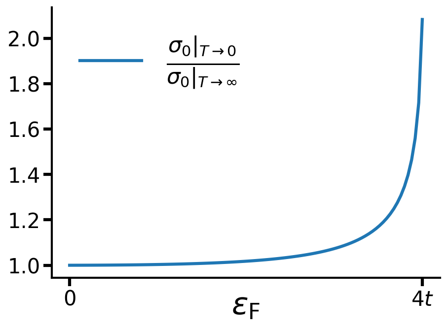
Figure 1: The ratio of the low- and high-T limits of the zero-field conductivity for the dispersion (61). Here, $\sigma_{0}\equiv\sigma_{xx}(B=0)=\sigma_{yy}(B=0)$. Note that $\varepsilon_{\rm F}=4t$ corresponds to half-filling, when the Fermi surface is most anisotropic.

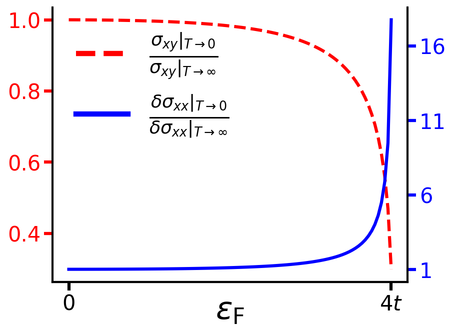
Figure 2: The ratio of the low- and high-T limits of the diagonal magnetoconductivity (solid line, right vertical axes) and Hall conductivity (dashed line, left vertical axes) for the dispersion (61).

V Conclusions

In this study, we have explored the Hall and diagonal magnetoconductivities arising from electron-electron (ee) interactions in a non-Galilean-invariant Fermi liquid. We showed that a $BT^{2}$ correction to the Hall conductivity and $B^{2}T^{2}$ correction to the diagonal magnetoconductivity are absent for an isotropic but non-parabolic spectrum in both 2D and 3D. The leading non-zero contributions scale in this case behave as $BT^{4}\ln T$ and $B^{2}T^{4}\ln T$, respectively, in 2D and as $BT^{4}$ and $B^{2}T^{4}$ in 3D. Although the components of the magnetoconductivity tensor depend on both $B$ and $T$, the diagonal magnetoresistance is absent for an isotropic system, as is also the case without ee interactions. The same scaling behavior, i.e, $BT^{4}\ln T$ for the Hall and $B^{2}T^{4}\ln T$ for the diagonal magnetoconductivity is also found for a convex surface in 2D, while the $BT^{2}$ and $B^{2}T^{2}$ scaling forms are recovered for a concave Fermi surface. We also analyzed the high-temperature regime, in which electron-electron scattering dominates over electron-impurity one, leading to a saturation in both zero-field and field-dependent corrections due to ee interaction. For an isotropic system, the conductivities in the high- and low-temperature limits coincide.

Appendix A Relaxation-time approximation for impurity scattering

The ei collision integral for point-like impurities-function is given by Eq. (12), which we copy below for the reader’s convenience

$$I_{\mathrm{ei}}=\frac{\langle f\rangle-f_{\mathbf{k}}}{\tau_{\mathrm{i}}}.$$ (62)

Therefore, the solution of the BE,

$$-e(\mathbf{v}\cdot\mathbf{E})n^{\prime}_{k}=\frac{\langle f\rangle-f_{\mathbf{k}}}{\tau_{\mathrm{i}}},$$ (63)

is defined only up to an arbitrary function of energy, $\langle f\rangle$. This does not affect the conductivity, as the $\langle f\rangle$ drops out from the current, but the distribution function itself remains undetermined. To fix this, we introduce a phenomenological collision integral of the relaxation-time approximation form

$$I_{\rm RTA}=\frac{n_{\mathbf{k}}-f_{\mathbf{k}}}{\tau},$$ (64)

where $n_{\mathbf{k}}$ is the equilibrium distribution function. Note that the integral of $I_{\rm RTA}$ over the directions of ${\bf k}$ at fixed energy is non-zero. Therefore, such a term cannot come from potential scattering, because the latter conserves the number of particles at given energy. At the same time $I_{\rm RTA}$ leads to energy dissipation, because $\int_{\bf k}\varepsilon_{\bf k}I_{\rm RTA}\neq 0$. Now the BE reads

$$-e(\mathbf{v}\cdot\mathbf{E})n^{\prime}_{k}=\frac{\langle f\rangle-f_{\mathbf{k}}}{\tau_{\mathrm{i}}}+\frac{n_{\mathbf{k}}-f_{\mathbf{k}}}{\tau},$$ (65)

which yields

$$f_{\mathbf{k}}=\frac{1}{\frac{1}{\tau_{\mathrm{i}}}+\frac{1}{\tau}}\left[e(\mathbf{v}\cdot\mathbf{E})n^{\prime}_{\mathbf{k}}+\frac{\langle f\rangle}{\tau_{\mathrm{i}}}+\frac{n_{\mathbf{k}}}{\tau}\right].$$ (66)

Averaging the last expression over angles, we find that $\langle f\rangle=n_{\mathbf{k}}$. Now the solution is unique

$$f_{\mathbf{k}}=n_{\mathbf{k}}+\frac{1}{\frac{1}{\tau_{\mathrm{i}}}+\frac{1}{\tau}}e(\mathbf{v}\cdot\mathbf{E})n^{\prime}_{\mathbf{k}}.$$ (67)

After this step, we can safely set $1/\tau=0$, which reproduces Eqs. (7) and (15).

Appendix B Symmetrized form of the electron-electron contribution to the conductivity

We assume that our system has both time-reversal and inversion symmetries. In this case, the scattering probability satisfies the microreversibility condition [28, 26]

$$W_{\mathbf{k},\mathbf{p}\leftrightarrow\mathbf{k^{\prime}}\mathbf{p^{\prime}}}=W_{\mathbf{k^{\prime}},\mathbf{p^{\prime}}\to\mathbf{k}\mathbf{p}}.$$ (68)

Next, indistinguishability of electrons implies that

$$W_{\mathbf{k},\mathbf{p}\leftrightarrow\mathbf{k}^{\prime},\mathbf{p}^{\prime}}=W_{\mathbf{k},\mathbf{p}\leftrightarrow\mathbf{p}^{\prime},\mathbf{k}^{\prime}}=W_{\mathbf{p},\mathbf{k}\to\mathbf{k}^{\prime},\mathbf{p}^{\prime}}=W_{\mathbf{p},\mathbf{k}\to\mathbf{p}^{\prime},\mathbf{k}^{\prime}}.$$ (69)

Finally, combining the last two properties, we obtain the third one

$$W_{\mathbf{kp\rightarrow k}^{\prime}\mathbf{p}^{\prime}}=W_{\mathbf{p}^{\prime}\mathbf{k}^{\prime}\rightarrow\mathbf{pk}}.$$ (70)

The first iteration of the BE with respect to magnetic field gives the following form of the correction to the Hall conductivity due to ee interactions

$$\delta\sigma^{ee,B}_{\alpha\beta} \propto \int_{{\bf k},{\bf p},{\bf k}^{\prime},{\bf p}^{\prime}}W_{\mathbf{k},\mathbf{p}\leftrightarrow\mathbf{k^{\prime}}\mathbf{p^{\prime}}}\varv_{\mathbf{k},\alpha}[u_{\mathbf{k},\beta}+u_{\mathbf{p},\beta}-u_{\mathbf{k^{\prime}},\beta}-u_{\mathbf{p^{\prime}},\beta}]\mathcal{D}_{{\bf k},{\bf p},{\bf k}^{\prime},{\bf p}^{\prime}}\equiv S.$$ (71)

where $\mathcal{D}_{{\bf k},{\bf p},{\bf k}^{\prime},{\bf p}^{\prime}}\equiv\delta({\bf k}^{\prime}+{\bf p}^{\prime}-{\bf k}-{\bf p})\delta(\varepsilon_{{\bf k}^{\prime}}+\varepsilon_{{\bf p}^{\prime}}-\varepsilon_{{\bf k}}-\varepsilon_{{\bf p}})n(\varepsilon_{\bf k})n(\varepsilon_{\bf p})\left[1-n(\varepsilon_{{\bf k}^{\prime}})\right]\left[1-n(\varepsilon_{{\bf p}^{\prime}})\right]$. Relabeling ($\mathbf{k}\leftrightarrow\mathbf{p}$) and $\mathbf{k^{\prime}}\leftrightarrow\mathbf{p^{\prime}}$), and using Eq. (69), we obtain:

$$S=\int_{{\bf k},{\bf p},{\bf k}^{\prime},{\bf p}^{\prime}}W_{\mathbf{p},\mathbf{k}\to\mathbf{k^{\prime}}\mathbf{p^{\prime}}}\varv_{\mathbf{p},\alpha}[u_{\mathbf{k},\beta}+u_{\mathbf{p},\beta}-u_{\mathbf{k^{\prime}},\beta}-u_{\mathbf{p^{\prime}},\beta}]\mathcal{D}_{{\bf k},{\bf p},{\bf k}^{\prime},{\bf p}^{\prime}}=\int_{{\bf k},{\bf p},{\bf k}^{\prime},{\bf p}^{\prime}}W_{\mathbf{k},\mathbf{p}\leftrightarrow\mathbf{k^{\prime}}\mathbf{p^{\prime}}}\varv_{\mathbf{p},\alpha}[u_{\mathbf{k},\beta}+u_{\mathbf{p},\beta}-u_{\mathbf{k^{\prime}},\beta}-u_{\mathbf{p^{\prime}},\beta}]\mathcal{D}_{{\bf k},{\bf p},{\bf k}^{\prime},{\bf p}^{\prime}}.$$ (72)

Next, we interchange $\mathbf{k}\leftrightarrow\mathbf{k^{\prime}}$ and $\mathbf{p}\leftrightarrow\mathbf{p^{\prime}}$, and apply Eq. (68), to obtain:

$$S=\int_{{\bf k},{\bf p},{\bf k}^{\prime},{\bf p}^{\prime}}W_{\mathbf{k^{\prime}},\mathbf{p^{\prime}}\to\mathbf{k}\mathbf{p}}\varv_{\mathbf{k^{\prime}},\alpha}[u_{\mathbf{k^{\prime}},\beta}+u_{\mathbf{p^{\prime}},\beta}-u_{\mathbf{k},\beta}-u_{\mathbf{p},\beta}]\mathcal{D}_{{\bf k},{\bf p},{\bf k}^{\prime},{\bf p}^{\prime}}=-\int_{{\bf k},{\bf p},{\bf k}^{\prime},{\bf p}^{\prime}}W_{\mathbf{k},\mathbf{p}\leftrightarrow\mathbf{k^{\prime}}\mathbf{p^{\prime}}}\varv_{\mathbf{k^{\prime}},\alpha}[u_{\mathbf{k},\beta}+u_{\mathbf{p},\beta}-u_{\mathbf{k^{\prime}},\beta}-u_{\mathbf{p^{\prime}},\beta}]\mathcal{D}_{{\bf k},{\bf p},{\bf k}^{\prime},{\bf p}^{\prime}}.$$ (73)

Finally, we interchange $\mathbf{k}\leftrightarrow\mathbf{p^{\prime}}$ and $\mathbf{p}\leftrightarrow\mathbf{k^{\prime}}$, and apply Eq. (70), to arrive at

$$S=\int_{{\bf k},{\bf p},{\bf k}^{\prime},{\bf p}^{\prime}}W_{\mathbf{p^{\prime}},\mathbf{k^{\prime}}\to\mathbf{p}\mathbf{k}}\varv_{\mathbf{p^{\prime}},\alpha}[u_{\mathbf{p^{\prime}},\beta}+u_{\mathbf{k^{\prime}},\beta}-u_{\mathbf{p},\beta}-u_{\mathbf{k},\beta}]\mathcal{D}_{{\bf k},{\bf p},{\bf k}^{\prime},{\bf p}^{\prime}}=-\int_{{\bf k},{\bf p},{\bf k}^{\prime},{\bf p}^{\prime}}W_{\mathbf{k},\mathbf{p}\leftrightarrow\mathbf{k^{\prime}}\mathbf{p^{\prime}}}\varv_{\mathbf{p^{\prime}},\alpha}[u_{\mathbf{k},\beta}+u_{\mathbf{p},\beta}-u_{\mathbf{k^{\prime}},\beta}-u_{\mathbf{p^{\prime}},\beta}]\mathcal{D}_{{\bf k},{\bf p},{\bf k}^{\prime},{\bf p}^{\prime}}.$$ (74)

Adding up Eqs. (71 - 74), we obtain:

$$S = \frac{1}{4}\int_{{\bf k},{\bf p},{\bf k}^{\prime},{\bf p}^{\prime}}W_{\mathbf{k},\mathbf{p}\leftrightarrow\mathbf{k^{\prime}}\mathbf{p^{\prime}}}[\varv_{\mathbf{k},\alpha}+\varv_{\mathbf{p},\alpha}-\varv_{\mathbf{k^{\prime}},\alpha}-\varv_{\mathbf{p^{\prime}},\alpha}][u_{\mathbf{k},\beta}+u_{\mathbf{p},\beta}-u_{\mathbf{k^{\prime}},\beta}-u_{\mathbf{p^{\prime}},\beta}]\mathcal{D}_{{\bf k},{\bf p},{\bf k}^{\prime},{\bf p}^{\prime}}$$ (75)

$$= \frac{1}{4}\int_{{\bf k},{\bf p},{\bf k}^{\prime},{\bf p}^{\prime}}W_{\mathbf{k},\mathbf{p}\leftrightarrow\mathbf{k^{\prime}}\mathbf{p^{\prime}}}\Delta\varv_{\alpha}\Delta u_{\beta}\mathcal{D}_{{\bf k},{\bf p},{\bf k}^{\prime},{\bf p}^{\prime}},$$

which is the form announced in Eq. (22) of the main text. A symmetrized form of the diagonal magnetoconductivity in Eq. (24) is derived along the same lines.

References

- Landau and Pomeranchuk [1936] L. Landau and I. Y. Pomeranchuk, On the properties of metals at very low temperatures, Ph. Zs. Sowjet. 10, 649 (1936).
- Abrikosov [1988] A. A. Abrikosov, Fundamentals of the Theory of Metals (Noth Holland, (1988).).
- Maslov et al. [2011] D. L. Maslov, V. I. Yudson, and A. V. Chubukov, Resistivity of a Non-Galilean–Invariant Fermi Liquid near Pomeranchuk Quantum Criticality, Phys. Rev. Lett. 106, 106403 (2011).
- Lin et al. [2015] X. Lin, B. Fauqué, and K. Behnia, Scalable resistivity in a small single-component Fermi surface, Science 349, 945 (2015).
- Collignon et al. [2019] C. Collignon, X. Lin, C. W. Rischau, B. Fauqué, and K. Behnia, Metallicity and superconductivity in doped strontium titanate, Annual Review of Condensed Matter Physics 10, 25 (2019).
- Lv et al. [2019] Y.-Y. Lv, L. Xu, S.-T. Dong, Y.-C. Luo, Y.-Y. Zhang, Y. B. Chen, S.-H. Yao, J. Zhou, Y. Cui, S.-T. Zhang, M.-H. Lu, and Y.-F. Chen, Electron-electron scattering dominated electrical and magnetotransport properties in the quasi-two-dimensional Fermi liquid single-crystal , Phys. Rev. B 99, 195143 (2019).
- Wang et al. [2020] J. Wang, J. Wu, T. Wang, Z. Xu, J. Wu, W. Hu, Z. Ren, S. Liu, K. Behnia, and X. Lin, T-square resistivity without Umklapp scattering in dilute metallic Bi2O2Se, Nature Comm. 11, 3846 (2020).
- Kumar et al. [2025] K. S. Kumar, D. Barbalas, R. Bhandia, D. Lee, S. Varshney, B. Jalan, and N. P. Armitage, Absence of two-phonon quasi-elastic scattering in the normal state of doped SrTiO3 by THz pump-probe spectroscopy (2025), arXiv:2501.15771 .
- Gurzhi et al. [1982] R. Gurzhi, A. Kopeliovich, and S. B. Rutkevich, Sov. Phys.–JETP 56, 159 (1982).
- Gurzhi et al. [1995] R. N. Gurzhi, A. N. Kalinenko, and A. I. Kopeliovich, Electron-electron momentum relaxation in a two-dimensional electron gas, Phys. Rev. B 52, 4744 (1995).
- Pal et al. [2012] H. K. Pal, V. I. Yudson, and D. L. Maslov, Resistivity of non-Galilean-invariant Fermi- and non-Fermi liquids, Lith. J. Phys. 52, 142 (2012).
- Ledwith et al. [2019] P. J. Ledwith, H. Guo, and L. Levitov, The hierarchy of excitation lifetimes in two-dimensional Fermi gases, Ann. Phys. 411, 167913 (2019).
- Rosch and Howell [2005] A. Rosch and P. C. Howell, Zero-temperature optical conductivity of ultraclean fermi liquids and superconductors, Phys. Rev. B 72, 104510 (2005).
- Rosch [2006] A. Rosch, Optical conductivity of clean metals, Annalen der Physik 15, 526 (2006).
- Maslov and Chubukov [2017] D. L. Maslov and A. V. Chubukov, Optical response of correlated electron systems, Rep. Prog. Phys. 80, 026503 (2017).
- Sharma et al. [2021] P. Sharma, A. Principi, and D. L. Maslov, Optical conductivity of a Dirac-Fermi liquid, Phys. Rev. B 104, 045142 (2021).
- Goyal et al. [2023] A. P. Goyal, P. Sharma, and D. L. Maslov, Intrinsic optical absorption in Dirac metals, Annals of Physics 456, 169355 (2023).
- Li et al. [2023] S. Li, P. Sharma, A. Levchenko, and D. L. Maslov, Optical conductivity of a metal near an Ising-nematic quantum critical point, Phys. Rev. B 108, 235125 (2023).
- Esterlis et al. [2021] I. Esterlis, H. Guo, A. A. Patel, and S. Sachdev, Large- theory of critical fermi surfaces, Phys. Rev. B 103, 235129 (2021).
- Guo [2023] H. Guo, Fluctuation spectrum of 2+1d critical fermi surface and its application to optical conductivity and hydrodynamics (2023), arXiv:2311.03458 [cond-mat.str-el] .
- Gindikin and Chubukov [2024] Y. Gindikin and A. V. Chubukov, Fermi surface geometry and optical conductivity of a two-dimensional electron gas near an Ising-nematic quantum critical point, Phys. Rev. B 109, 115156 (2024).
- Collignon et al. [2021] C. Collignon, Y. Awashima, Ravi, X. Lin, C. W. Rischau, A. Acheche, B. Vignolle, C. Proust, Y. Fuseya, K. Behnia, and B. Fauqué, Quasi-isotropic orbital magnetoresistance in lightly doped , Phys. Rev. Materials 5, 065002 (2021).
- Ziman [2001] J. Ziman, Electrons and Phonons (Oxford University Press, 2001).
- Mirlin and Wölfle [1997] A. D. Mirlin and P. Wölfle, Composite Fermions in the Fractional Quantum Hall Effect: Transport at Finite Wave Vector, Phys. Rev. Lett. 78, 3717 (1997).
- Gurzhi [1968] R. N. Gurzhi, Hydrodynamic effects in solids at low temperature, Phys. Usp. 11, 255 (1968).
- Gantmakher and Levinson [1987] V. F. Gantmakher and Y. B. Levinson, Carrier Scattering in Metals and Semiconductors (North-Holland, Amsterdam, 1987).
- Ch’iang and Eremenko [1966] Y. N. Ch’iang and V. Eremenko, Pecularities of the temperature dependence of electric conductivity of aluminum at helium temperatures, JETP Lett 3, 447 (1966).
- Sturman [1984] B. I. Sturman, Collision integral for elastic scattering of electrons and phonons, Sov. Phys.-Uspekhi 27, 881 (1984).