Auto-Associative Memories for Direct Signaling of Visual Angle During Object Approaches
Abstract
Being hit by a ball is usually not a pleasant experience. While a ball may not be fatal, other objects can be. To protect themselves, many organisms, from humans to insects, have developed neuronal mechanisms to signal approaching objects such as predators and obstacles. The study of these neuronal circuits is still ongoing, both experimentally and theoretically. Many computational proposals rely on temporal contrast integration, as it encodes how the visual angle of an approaching object changes with time. However, mechanisms based on contrast integration are severely limited when the observer is also moving, as it is difficult to distinguish the background-induced temporal contrast from that of an approaching object. Here, I present results of a new mechanism for signaling object approaches, based on modern content-addressable (auto-associative) memories. Auto-associative memories were first proposed by Hopfield in 1982, and are a class of simple neuronal networks which transform incomplete or noisy input patterns to complete and noise-free output patterns. The memory holds different sizes of a generic pattern template that is efficient for segregating an approaching object from irrelevant background motion. Therefore, the model’s output correlates directly with angular size. Generally, the new mechanism performs on a par with previously published models. The overall performance was systematically evaluated based on the network’s responses to artificial and real-world video footage. A gentle introduction to the key ideas of this paper is available on Youtube.
Acknowledgements
This study was financially supported by grant PGC2018-099506-B-I00 and PID2022-142599NB-I00 from the Spanish Government.
1 Introduction
Detection of collision threats through visual information is vital for many organisms [27]. When an observer (e.g. a robot or an organism) does not move, tracking an approaching object is a straightforward computational exercise. However, when the observer is moving (and looking) straight ahead [15], all objects in its field of view appear to collide. The additional movement due to the self-motion of the observer is referred to as background motion or background movement. With background motion, a computational challenge is to distinguish objects that will eventually collide with the observer from those that will pass by. In other words, any collision detection system should filter out background motion such that it responds to any colliding object in the same way as it would without background movement.
It is worthwhile to understand the neuronal circuitry of the locust’s lobula giant movement detector (LGMD) neurons, as they reliably respond to approaching objects in depth, even in the presence of background motion [47, 41, 48]. Two types of LGMD neurons are distinguished by their responses to luminance contrast: LGMD1 responds to both lighter and darker objects than the background [41], while LGMD2 responds only to darker objects [49]. When probing the LGMD1’s response to object approaches against a drifting grating, a reduction in response occurs [41]. For the LGMD2, the reduction is less pronounced for intermediate drifting frequencies111The (effective) drifting frequency of a grating increases both with its spatial frequency and temporal frequency. [49].
The effect of background suppression on LGMD responses is further highlighted by showing locusts selected parts of the Star Wars movie [41] or dashcam videos showing car crashes and less harmful traffic footage [17].
Computational models for the LGMD usually start with calculating the difference between two consecutive (gray-level) video frames (temporal contrast or isotropic optical flow). Temporal contrast extraction is a frame-rate based implementation of event-based signal processing in the sense that a signal is only generated if a movement occurs from one frame to the next [53, 14].
For an approaching object in the absence of background motion, the spatial sum of temporal contrast (SOC) correlates with the object’s angular velocity (Figure 1). Angular velocity refers to the rate of change of the visual angle. For driving LGMD responses, (temporal) contrast edges were identified as a relevant feature [48], when these edges increase in size and velocity in concert with an approaching object. Activity related to temporal contrast provides excitatory input to the LGMD.
In parallel, inhibition to neighboring spatial positions in retinotopic space is generated (lateral inhibition for short). If excitatory activity is eventually to build up in the LGMD neuron and trigger a response, then excitation must escape the inhibitory wavefront. This occurs for approaching objects, because the closer the object gets, the bigger will be its image projected on the retina (angular size), and the faster its edges will grow (angular velocity) [39, 42]. Lateral inhibition therefore implements a predictive mechanism for non-approaching objects [28]
Two further inhibitory mechanisms may act to avoid undesired responses and improve the suppression of background motion: (i) large-field feedforward inhibition is activated upon a large increment of SOC from one time step to the next; this prevents corresponding activity from building up in the LGMD. For example, such sudden increases can occur in response to changes in the viewing direction and/or self-motion.
(ii) The mean LGMD activity across the recent past can also be subtracted from the instantaneous LGMD activity. Along with adequate thresholding of the LGMD response the baseline excitation due to background motion is removed.
If the inhibitory pathways have lowpass characteristics in time, then persistence of past activity in these channels decreases responsiveness and object approaches may be missed.
This problem can be solved by increasing the number of parallel inhibitory channels, such that the activity in each channel is kept low on the average. For example, temporal contrast can constitute parallel ON (positive values of temporal contrast) and OFF (negative values) channels [28]. Thus, “sparsification” reduces possible interferences between residual inhibition from past events and the excitation from the present input.
Inspired by the locust visual system, a fairly popular class of (SOC-based) computational models and algorithms have been proposed and are under ongoing development (e.g. [39, 4, 29, 28, 34, 59, 12, 6, 11, 33]). The results of three instances of this class of models will be used as reference to compare them with the proposal of this paper.
The model proposed in this paper takes a rather unusual approach, using a modern Hopfield network, whose output correlates with the angular size of an approaching object. Our focus is on background suppression. Numerical experiments suggest that Hopfield-based collision signaling has a comparable performance to (SOC-based) LGMD models. In particular, the Hopfield model can signal an object approach when plain SOC does not show a corresponding increase in activity at the end of an approach. This implies that a SOC-based LGMD model would miss the approaching object. However, for certain video sequences the Hopfield model is outperformed by the LGMD models. These limitations are are linked to the specific nature of information processing in both models and will be described further down.
2 Material and Methods
2.1 Hopfield Networks
Throughout the paper, capital letters denote matrices, and lower case letters represent column vectors. Vectors are denoted either by (where the index is a label), or as (where the index refers to the element of the -th row of ). In order to denote the -th element of , we use .
A Hopfield network is an auto-associative memory where the stored pattern vectors constitute attractors provided that a Lyapunov (or energy) function exists. Thus, if the network is set to some initial state , it will evolve to a (local) minimum of the Lyapunov function. The originally proposed Hopfield network admits only binary states and pattern [21, 22], and has a comparatively low storage capacity. Correlations between stored pattern reduce storage capacity further and typically generate retrieval states which are linear combinations of the correlated pattern.
222Some illustrations for the classical Hopfield network with input versus retrieved pattern can be found via the following URLs:
(i) adding noise to the input;
(ii) rotating the input;
(iii) using contours.
For all illustrations, the query pattern was stored in the Hopefield network.
Dense associative memories (aka modern Hopfield networks) extend classical Hopfield networks such that storage capacity grows super-linearly [31] or even exponentially [8] with the number of network units. This is achieved by using nonlinear functions with a narrow support around the stored pattern, leading to smaller basins of attraction.
The binary pattern restriction has been overcome recently [37, 58, 32], while maintaining exponential storage capacity and one (or few) update steps until convergence
333Illustrations of input versus retrieved pattern using a modern associative memory:
(i) adding noise to the input;
(ii) rotation (gray-scale);
(iii) rotation (binary input);
(iv) using contour images.
For all illustrations, the query pattern was stored in the pattern memory..
Accordingly, one update rule is based on the -function, which essentially corresponds to the attention mechanism of transformer networks [56],
| (1) |
The continuous state of the network (”query”) is ; is the inverse temperature. The continuous-valued pattern vectors , are stored as columns of the pattern matrix . For an auto-associative memory, (in transformers, is the value matrix).
The -function is defined as
| (2) |
The argument of of Equation (1) computes the inner product of the state with all stored pattern . Assuming proper pattern normalization, the resulting vector can be interpreted as the initial probability distribution across the stored pattern . If all pattern in are well separated (i.e., no two pattern are similar to each other)444By defining separation as , Theorem 5 in ref. [37] states that the retrieval error for pattern decreases exponentially with ., then the pattern with the highest probability typically is selected after one iteration of Equation (1), while all others are suppressed. However, correlations among some of the stored patterns can result in the retrieval of meta-stable states [37]: Instead of one retrieved pattern, a mixture of similar pattern may appear, because more than one element of is close or equal to the maximum. This can be mitigated by setting to a bigger value, although this may result in numerical issues.
2.2 A Modern Hopfield Network for Collision Detection

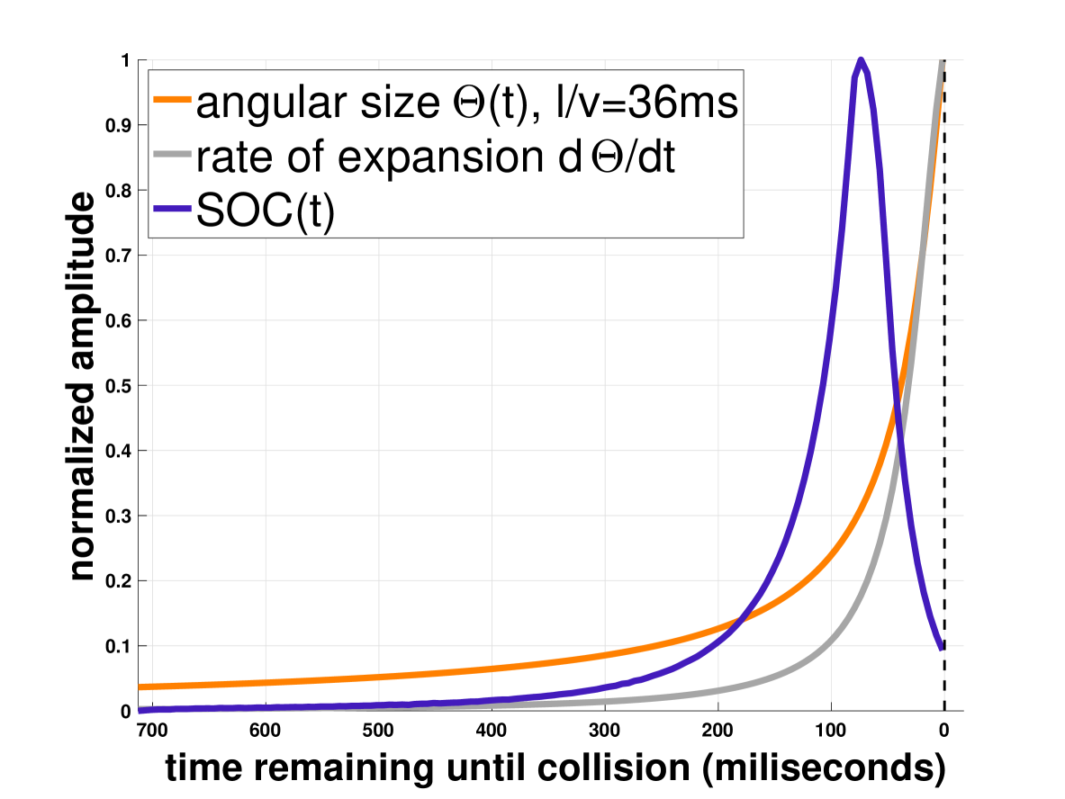
In this section, an algorithm (computational model) for detecting objects that approach the observer on a direct collision course is defined. We emphasize reproducibility by providing step-by-step instructions. The selected parameter values were determined through a systematic exploration of the parameter space with the goal of achieving “good” overall performance with a set of benchmark videos. Good performance means that the model’s response follows the angular size of the approaching object (Figure 1): when the object is far away, the response should be small or zero, and when the object is close, the response should increase almost exponentially, while being as smooth as possible. Specifically, the benchmark set consisted of four artificial and four real-world video sequences.
2.2.1 Video Frame Processing

Let be a gray-level video frame with rows and columns at discrete time . Video frames with can be symmetrically embedded in a square matrix with a constant luminance (e.g. ) such that the resulting frame has an equal number of rows and columns, respectively. Proceeding so, however, may compromise the detection of potential collisions. Alternatively, the frames can be cropped such that .
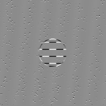
Let be a convolution kernel implementing a modified version of the Sobel-Feldman operator (cf. [46]) for enhancing the horizontal edges of (Figure 2b),
| (3) |
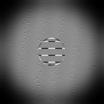
A region-of-interest (mask) is constructed by (i) creating a white disk (luminance ) on black background (luminance ) with radius , and (ii) blurring the disk with a Gaussian kernel with standard deviation pixel (Figure 2c). Applying the mask to the video frames improves specifically performance for videos with strong background motion. Videos without background motion would not benefit much from the mask. Neither the value of nor the degree of spatial blur turned out to be critical for the considered video footage. The value of was selected from plus “no mask at all”. The degree of spatial blur was selected from .
Figure 2d shows the final result of video processing: At each time , frame is first convolved with (symbol ””) and then element-wise multiplied with (Hadamard product, symbol ””),
| (4) |
2.2.2 Image to Vector Conversion
In order to be used with modern Hopfield networks, (image) matrices ( video frames and template pattern ) have to be converted into vectors ( and , respectively) with . All vectors are assumed to have the following properties:
-
1.
(index mapping)
-
2.
(centering at zero)
-
3.
(normalization)
The first property states that all matrices have to be converted into vectors in the same way (i.e., with identical index mapping). The second property is implemented by subtracting the mean . The third property is implemented by dividing by the Euclidean norm . Thus, all vectors are unit vectors.
2.2.3 Pattern Memory
Pattern vectors are columns of pattern matrices (pattern memory , cf. Equation (1)). Specifically we have two separate pattern memories
| (5) | |||||
| (6) |
This implies two corresponding instances of Equation (1), one with , and another one with .
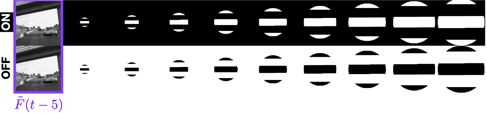
Let be the pattern vector from converting the processed video frame with the properties defined in Section 2.2.2. Then, . That is, the first column of both pattern memories is dynamically updated with a by five time steps delayed video frame (Figure 3)555For initialization, the video sequence may be started at , or for . The delay by five time steps was selected from , , and . We tried furthermore an adaptive delay, but discarded it because it did not lead to a significant improvement over the fixed delay.. The remaining columns of and do not change with time and are laid out as follows.
Let be a gray-level template image with rows and columns, respectively. The default template image is a disk with an overlaid horizontal grating (2 cycles per image) as shown in Figure 3. Notice that the grating orientation matches the orientation of the Sobel-Feldman operator for processing the video frames (Equation (3)).
In total, versions of the template image are generated, with varying disk diameters of pixel, starting with a scale-factor of and increasing to in steps of 666This heuristics for has been found by trying starting values combined with increments . Results are not significantly different for most videos if instead we start with a constant disk diameter of seven pixel and use increments of ..
Subsequently, the edges of each template image are enhanced with the Laplacian operator,
| (7) |
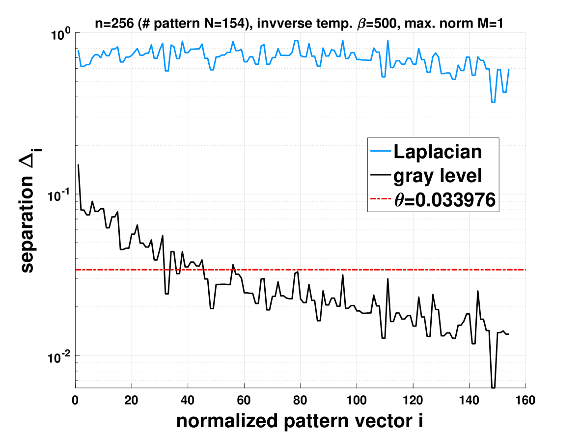
and converted into vectors with the properties defined in Section 2.2.2. The are stored in from column to . The inverse versions are stored in . Therefore, the size of and is , with and (one more because of ). Compared with storing gray-level images, their edge-enhanced counterparts are better separated (Figure 4). Notice that the pattern matrices have to be specifically build according to video frame size .
Several combinations of functions operating on the pixels of the video frames were tried for Equations 3 and 7, respectively:
-
1.
Luminance (unprocessed video frames)
-
2.
Laplacian
-
3.
Difference of successive video frames (temporal contrast)
-
4.
Difference between the gradient magnitudes of successive video frames
-
5.
Odd-symmetric Sobel-Feldman operator with orientations
-
6.
Even-symmetric Sobel-Feldman operator ( LDL kernel, where “L” (light) means positive values of the filter kernel and “D” (dark) stands for negative values) with orientations
-
7.
Oriented temporal contrast along directions using the following calculations: (i) Temporal contrast; (ii) convolution of absolute temporal contrast with an oriented and even-symmetric Sobel-Feldman kernel; (iii) spatial blurring the result of the previous step with an asymmetric Gaussian kernel (standard deviation and , respectively) with perpendicular orientation (iv) multiplication with temporal contrast.
When oriented operators were used for both video frame processing and pattern memory processing, then their respective orientations were matched . Furthermore, “temporal contrast” for the pattern memory is defined as the difference .
2.2.4 Pattern Retrieval
The proposed algorithm proceeds frame-wise where denotes the current video frame. The current video frame is processed and converted into . The queries are initialized with and , where denotes the iteration number of the update rules
| (8) | |||||
with the probability distributions and , respectively, defined as
| (9) | |||||
The inverse temperature is set to , and Equation (8) is iterated until or (analogous for ). As mentioned in Section 2.1, the update usually converges after one iteration for well separated pattern (Figure 4).
The inverse temperature cannot be increased much further for an improved suppression of meta-stable states. The reason is that numerical overflow due to exponentiation may occur777If numerical problems occur, then one could replace Equation (2) by a ”fail-safe” version along with . Doing so would also suppress meta-stable retrieval states..
2.2.5 Conversion of Retrieval States into Neuronal Activity
The retrieved pattern are not used any further (except for illustration). The label of the winning pattern (or their mean in case of a meta-stable retrieval state) is directly taken as activity. Let be a row vector denoting the column number of pattern memories and , respectively. The (scalar) activities and are defined as the inner products
| (10) | |||||
The higher the activity, the greater the disk diameter of the retrieved pattern. Therefore, activities are proportional to the angular size of an approaching object. The lowest activity is obtained if the delayed video frame is retrieved. Since the activity is usually very spiky, online smoothing (lowpass filtering) is applied,
| (11) | |||||
This equation is a discrete representation of a leaky integrator neuron (cf. Text S8 of [27]). The memory coefficient is a constant that sets the degree of smoothing; is the state variable and the smoothed output; is the original signal (filter input). If is close to one (equivalent to a small leakage conductance), then the input is mainly integrated and thus strongly smoothed. However, more smoothing translates into a greater delay (i.e., phase lag) between input and output. This has to be taken into account for real-time applications of the proposed algorithm. Accordingly,
| (12) | |||||
where and & are the smoothed activities ( filter output). Finally, the ON and OFF signals are combined by multiplication [5, 13, 25, 26],
| (13) |
Notice that because . This is to say that because the minimum activity of either channel is nonzero, will reflect the activity of at least or .
2.3 Benchmark Models
The results of the “Hopfield” model as introduced above will be compared to three models which are based on temporal contrast extraction (”SOC-based models”). These are briefly outlined in what follows.
2.3.1 A neural model of the locust visual system for detection of object approaches with real-world scenes [28] (“Advanced”)
The model “Advanced” splits temporal contrast into parallel ON and OFF pathways. The ON channel encodes luminance increments from one video frame to the next, the OFF channel decreasing luminance. Lateral inhibition is implemented by self-limiting diffusion layers. Diffusion is self-limiting because it curtails the excitatory activity by which it is fed. Let be the halfwave rectified activity of the ON-channel, and that of the OFF-channel. The channels are combined by
| (14) |
where and filter memory . Different to the “Hopfield” model, and of “Advanced” can be zero. The first term thus implements a logical “AND” gate, which would be zero for example for a white disk approaching against a black background, or an approaching bird against a clear sky. In order to obtain non-zero activity in the latter cases, the second term was included.
2.3.2 Self-Supervised Learning of the Biologically-Inspired Obstacle Avoidance of Hexapod Walking Robot [6] (“CizFai19”)
The “CizFai19”-model computes LGMD1 responses to both lighter and darker objects than the background [41]. It was implemented following the equations seven (“photoreceptor layer”, i.e. temporal contrast) to eleven (“summation layer”) of Section 3.3. in ref. [6]. Equation twelve eventually sets all units of the summation layer to zero if . Since the threshold (originally a scalar constant) “ has to be set experimentally in such a way to avoid saturation of the LGMD output”, here I replaced it by an adaptive mechanism controlled by temporal contrast activity888The model is invariant with respect to the range of luminance values. ,
| (15) |
where is scalar, the size of the gray-level video frame is and the filter memory coefficient is set to (cf. Equation (11) above). Subsequently, all summation layer units with are set to zero. For computing the model’s output (i.e., the LGMD membrane potential), let . Then:
| (16) |
subject to another adaptive threshold that varies according to
| (17) |
with filter memory coefficient .
2.3.3 A Robust Collision Perception Visual Neural Network With Specific Selectivity to Darker Objects [11] (“FuHuPe20”)
The “FuHuPe20”-model computes LGMD2 responses to darker objects than the background [49]. As the previous model, it also uses temporal contrast at its front end. Since the complementary ON-channel is missing, I created it by using a second instance of the model with inverse temporal contrast as input. After conducting tests with a variety of video footage, the (free) frame rate parameter of the model was set constant to Hz. The spiking output (i.e., equation 27 in ref. [11]) of both model instances and , respectively, was combined according to Equation (14) with and filter memory . Lowpass filtering of the spikes essentially mirrors the membrane potential of a (hypothetical) neuron postsynaptic to the LGMD.
3 Results
3.1 Principal Characteristics and Limitations
In this section, we explore some of the main characteristics of the “Hopfield”-model by means of artificial video sequences. The sequences can be fully parameterized in terms of physical approach variables (cf. Figure 1), object type (e.g., spatial frequency and orientation of the rectangular grating that forms the texture of the approaching disk), and background (e.g. a sine wave grating with a certain spatial frequency, orientation, and drifting speed). Drifting speed was implemented as the time dependent phase of the grating where is the frame number and with Hz.
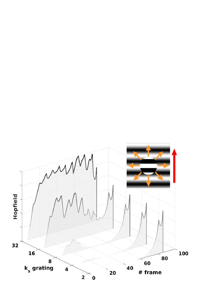
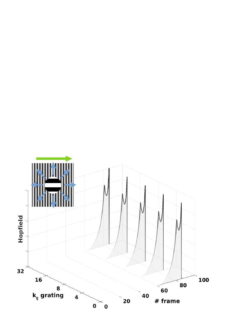
The determining factor for constructing a worst case scenario for the “Hopfield”-model is the orientation of the background grating. When the grating is horizontally oriented (as the template pattern shown in Figure 3), then pattern retrieval is compromised (i.e., interference occurs) for certain combinations of the grating’s drifting speed and spatial frequency. Similarly, variation of the spatial frequency and orientation of the approaching disk’s texture only impairs pattern retrieval if the background grating is horizontally oriented. In contrast, variations of disk or grating parameters would not interfere with pattern retrieval when the grating is vertically oriented: Corresponding data are only insignificantly different from to those shown in Figure 5b.
Assuming a horizontally oriented background grating, the critical parameter is its spatial frequency (Figure 5a): Increasing will increase interference and therefore overall retrieval activity. For , retrieval activity will no longer increase in the final approach phase. These properties of the “Hopfield”-model are linked to high-pass filtering: The “Hopfield”-model predominantly uses the high spatial frequencies of video frames and pattern templates (Equations (4) and (7), respectively).

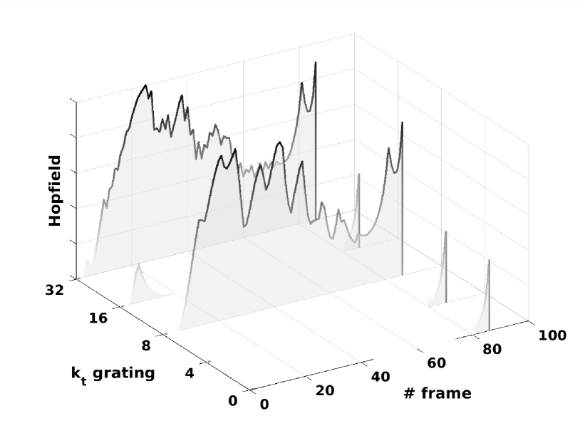
For suitable combinations of and , ”resonance” effects due to temporal aliasing can be observed (Figure 6b): The curves for Hz have less overall activity than those for Hz. Thus, a nearly similar plot to Figure 5a would result when using Hz instead of Hz (not shown).
With a horizontally oriented grating as background, increasing the spatial frequency of the approaching disk generates less overall activity, especially in the initial approach phase (not shown). The resonance pattern observed with respect to is consistent with the one described above. With respect to the orientation of the approaching disk, activity in the initial approach phase tends to decrease close to the horizontal orientation. Again, for a vertically oriented background grating, retrieval activity is largely independent of disk spatial frequency and orientation.
Figure 6a shows the sum-of-temporal-contrast (SOC, cf. Figure 1) as a function of . Since SOC is isotropic, there are no effects of disk or grating orientation. As SOC is a temporal high-pass filter, increasing increases SOC activity. Conversely, SOC is largely independent of (not shown).
With respect to the spatial frequency of the approaching disk’s texture, SOC activity in the final approach phase increases with increasing spatial frequency. Thus, the final peak of the curves for and Hz in Figure 6a could be recovered by increasing the disk’s spatial frequency. No significant changes in the SOC curves occur when varying the disk orientation (not shown).
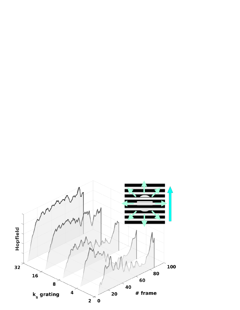

When the drifting grating partially occludes the approaching disk (Figure 7a), more spurious activity (interference) is generated than with the drifting grating in the background (Figure 5a). As before, interference only occurs when the orientations of the grating and the template pattern match (Figure 3): a foreground grating with vertical orientation would produce similar results to those shown in Figure 5b for all spatial frequencies and drifting speeds .
The spurious activity generated by a rotating background grating depends on both the rotation speed (in degrees per frame) and spatial frequency . Generally, low rotation speeds (in the examined range from to degrees per frame) and higher spatial frequencies generate more interference. For low rotation speeds, interference can only occur if the grating orientation at some time is the same as that of the template pattern. Conversely, at high speeds, phase aliasing
may periodically generate spurious activity (see curve for in Figure 7b). However, for all combinations of rotation speed (in the range of to degrees per frame) and spatial frequency of the grating, the activity increase in the final approach phase remains clearly distinguishable from the spurious activity generated before.

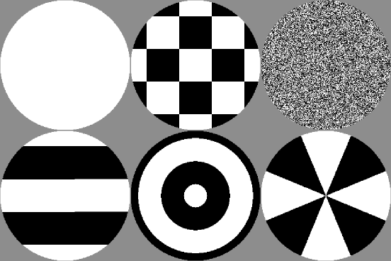
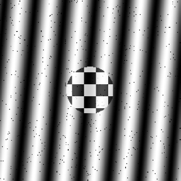
Can the “Hopfield”-model also signal approaching disks with a different pattern than the striped disk used as a template pattern (Figure 3)? To investigate this, we studied model responses with five additional object patterns (Figure 8b) approaching over background gratings of various drifting velocities and orientations. For a vertically oriented grating, the model responded to all object patterns except for the starburst grating. The highest response amplitudes were obtained for the uniform disk and the linear (default) grating. The chessboard pattern and the circular grating generated smaller amplitudes, while the smallest amplitude was obtained for the noise patch. Responses did not significantly depend on the drifting speed or spatial frequency of the grating. When using an approaching object with a square shape instead of a disk, similar responses were obtained for all six pattern.
When increasing the spatial frequency of the textured disks (except of the noise patch), then responses with more spurious activity are generated, and any response peak in the final approach phase gets smaller or disappears. This implies that the detection of the corresponding approaching disk becomes virtually impossible. As to SOC, the starburst grating and the uniform disk will generate practically no activity increase in the final approach phase (not shown). All other types of approaching disks will generate a distinct peak in the final approach phase. The peaks vary with spatial frequency, but nonetheless remain clearly visible (not shown).
With a diagonally oriented background grating, the gross response pattern as a function of drifting speed is analogous to that shown in Figure 6b: For drifting speeds and Hz, very narrow response peaks are produced (i.e., very late response onset). For and Hz, responses do not contain spurious activity, but their onset occurs later than with the horizontal grating. For and Hz, response onset is similar to the horizontal grating, but responses are contaminated with small amounts of spurious activity.
Responses to the horizontally oriented grating resemble those of the diagonal grating, but with significantly more spurious activity generated at Hz (as shown in Figure 8a) and Hz.
How do SOC responses behave with the mentioned object patterns and background grating configurations? SOC responses do not vary significantly with grating orientation and object shape (square vs. circular). Importantly, SOC shows a response peak in the final approach phase with the starburst pattern, where the latter and the uniform pattern have the smallest response amplitude compared to the rest. These peaks generated with the starburst and uniform object patterns are distinguishable up to Hz, and from Hz, the activity generated by the background grating becomes larger, causing these peaks to disappear. The response peak of the approaching linear (default) disk disappears for Hz. The SOC peaks of all other types of disks are eventually gone at Hz.
3.2 Model Shootout with Artificial Videos
The results of the sum of temporal contrast (SOC) and the “Hopfield”-model from the previous section can be attributed to their respective filtering characteristics: SOC is a temporal high-pass filter, and strong background movement can interfere with the detection of an approaching object. The “Hopfield”-model, meanwhile, uses spatial high-pass filtering and its performance depends critically on whether the background has a similar structure as the template pattern. If it does, spurious retrievals can be generated, making it difficult to detect the approaching object.
In this section, we compare the responses of the “Hopfield”-model and SOC with three other models that are based on temporal contrast (”SOC-based models” for short). These are “FuHuPe20” (Section 2.3.3 [11]), “CizFai19” (Section 2.3.2 [6]), and “Advanced” (Section 2.3.1 [28]).
As each of the models covers a different range of output values, their responses had to be normalized in order to be displayed in a single figure. Specifically, the output of the “Hopfield”-model depends on the number of stored patterns . Because of Equation 13, the output can therefore vary between one and . The displayed curves were scaled by times a factor that is specified in the figure legends where applicable.
For “FuHuPe20”, we filtered the output spikes (cf. Section 2.3.3) which vary from zero to two. For displaying, we accordingly divided the filtered output by two.
The rest of the curves (including SOC and the visual angle ) were first divided by their respective maximum and subsequently multiplied by the maximum response between scaled “Hopfield” and scaled “FuHuPe20”.

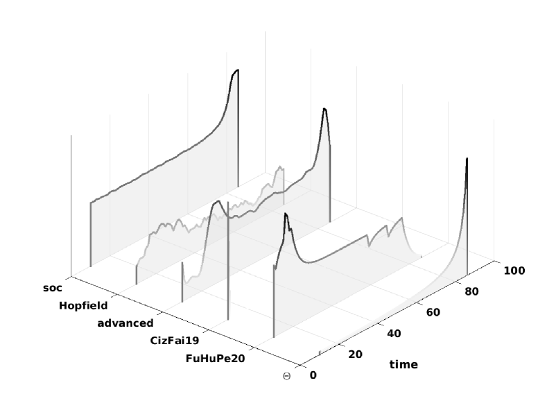
Figure 9 juxtaposes model responses for two types of approaching objects (uniform disk and noise patch) against a background of dynamically varying white noise. Luminance of the uniform disk was set to be identical to the spatio-temporal mean of the background, that is . This is likely a situation that would never be encountered in real-world applications, and it is even hard for humans on a calibrated computer monitor to perceive the approaching object before it nearly covers the entire frame. The simulations suggest that it is difficult for the tested models as well. With the uniform disk, only the “Hopfield” -model reveals an activity increase in the final approach phase. SOC stays saturated until the uniform disk grows large enough such that it occludes the background. This causes the activity decrease of SOC in the final approach phase. As a consequence, none of the SOC based model signals the approaching uniform disk.
A different situation is at hand with the approaching noise patch (third pattern of Figure 8b), where SOC shows an activity increase with time. Nevertheless, this increase is not mirrored in the responses of the SOC-based models except of “Advanced”. “Hopfield”, on the other hand, shows merely a moderate increase.

How does the output of the various models depend on the location of the focus of expansion (FOE)? Figure 10a shows SOC which represent the input to the models “Advanced”, “CizFai19”, and “FuHuPe20” as a function of the horizontal position of the FOE. The output of these SOC-based models follow their input, where each model’s response occurs later with increasing displacement of the FOE from the center of the video frames. This behavior is consistently observed irrespective of background luminance and object pattern.
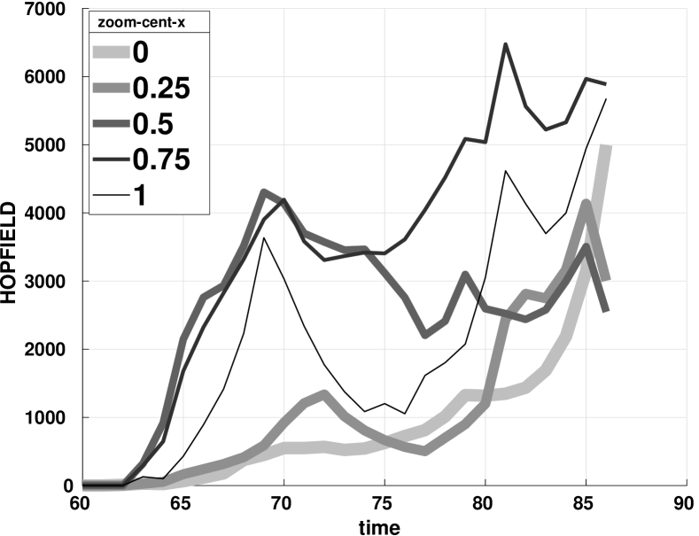
In contrast, the output of the “Hopfield”-model is influenced by background luminance and object pattern. For example, the highest response amplitudes are generated for an uniform white or black background. The closer the background luminance to medium gray, the smaller the “Hopfield”-responses. Similarly, an approaching object with uniform luminance (e.g. a texture-less white disk) produces higher responses with an onset at an earlier time than a patterned object (e.g. a disk with checkerboard pattern). When moving the FOE horizontally towards the frame boundary, “Hopfield”-responses tend to increase stronger at earlier times compared to a centered FOE (Figure 10b). Nevertheless, the time of the response onset does not change significantly.
3.3 Real-World Footage
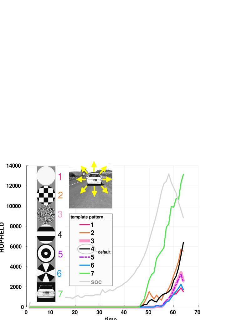
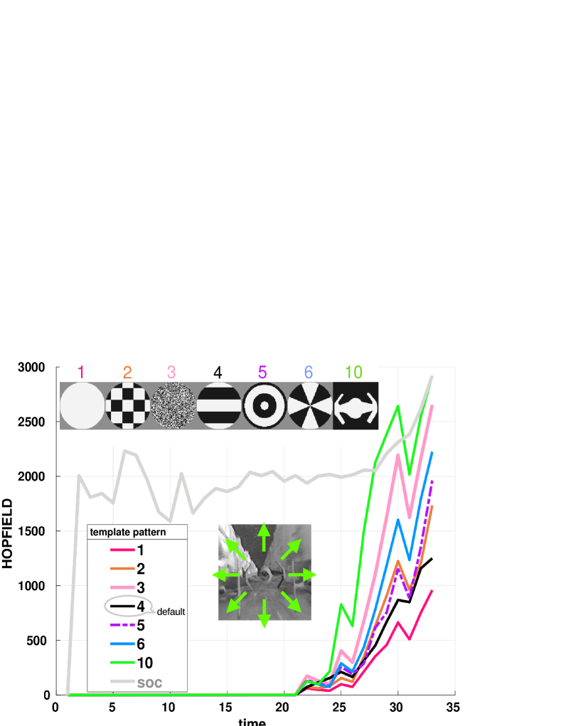
In this section model responses to four representative videos are compared with each other. Firstly, Figure 11 shows responses of the “Hopfield”-model along with the sum of temporal contrast (SOC) for different template patterns. The default template pattern is a horizontally-striped disk (Figure 3), which gave the best overall results with a set of benchmark videos. Therefore, the performance of the “Hopfield”-model may depend on the specific video under consideration. Figure 11 shows that the optimal template pattern for each video is that which achieves the highest correlation with the approaching object. This is a car for the Mercedes Sequence, and the central space ship for the Star Wars Sequence. The rest of the selected template pattern produced responses with lower amplitudes. However, the next best (artificial) templates are not necessarily identical across different videos: While for Mercedes these are the checkerboard disk and the default template, respectively, for Star Wars we have the noise patch and the starburst grating, respectively.
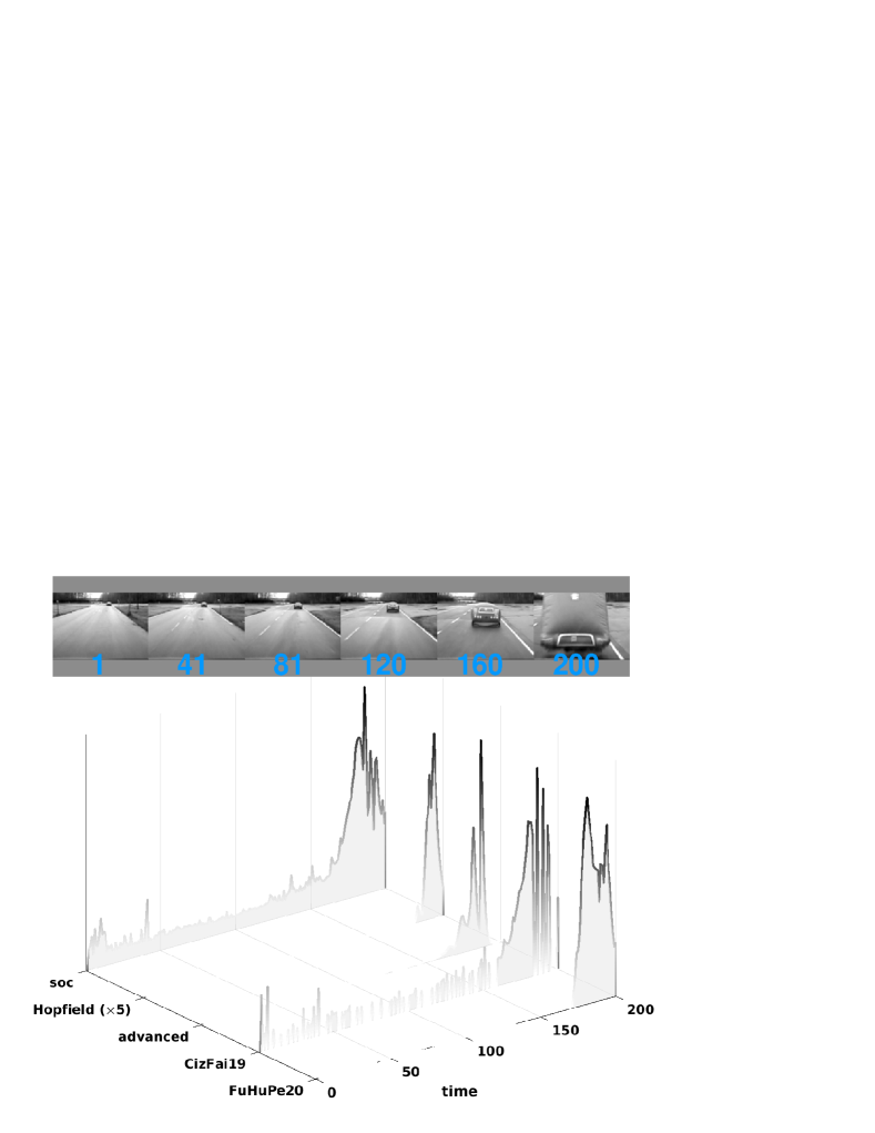
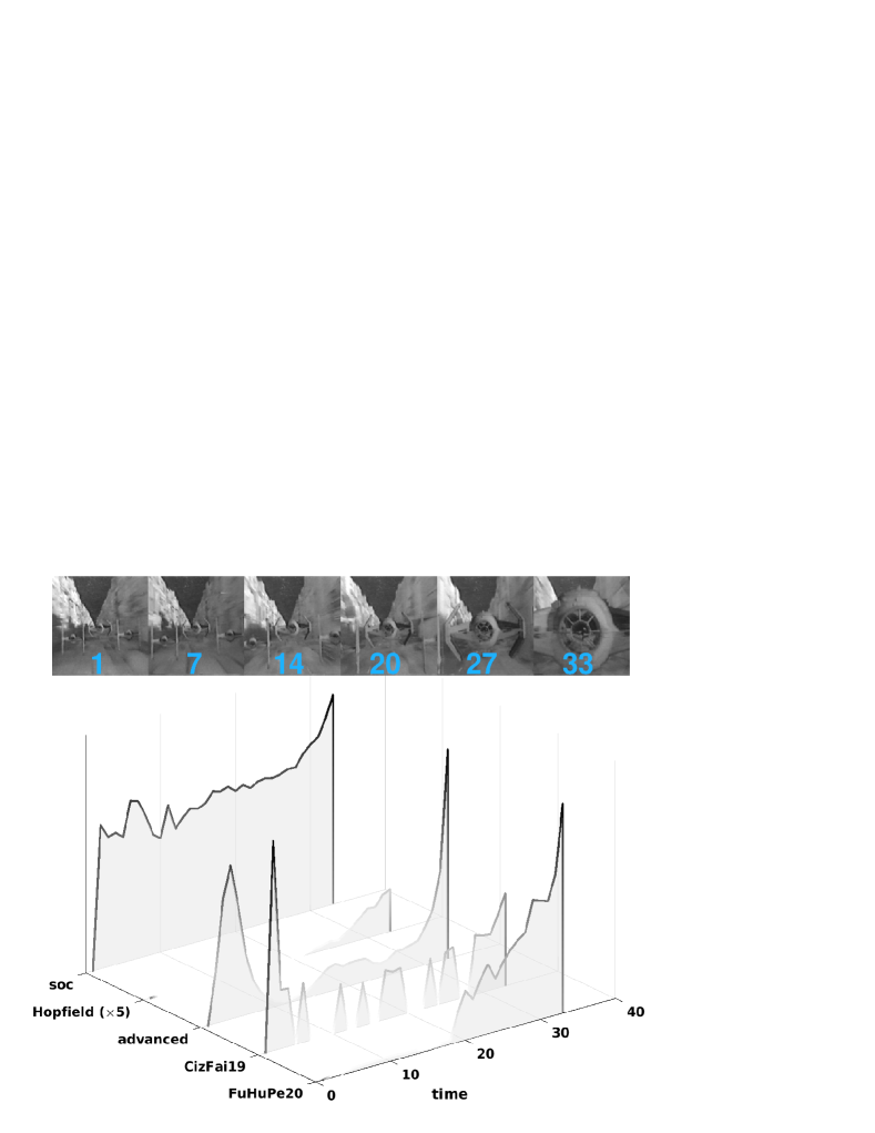
Figure 12a juxtaposes responses of all models to the Balloon Car Sequence. The video has modest background movement and shows a crash with an inflated mockup car. The background movement translates into non-zero SOC responses throughout the approach, and is well suppressed by the models “FuHuPe20”, “Advanced”, and “Hopfield”. The response onset of “FuHuPe20” and “Advanced” coincide with the activity increase of SOC, where the latter two models respond earlier than “Hopfield” does. In summary, all considered models signal the approach to the stationary balloon car.
Figure 12b shows corresponding results for the Star Wars Sequence, where three spaceships are approaching the observer. The observer looks into the opposite direction of his or her movement. As a consequence, the background moves opposite to the approaching space ships as well. This benchmark video is challenging due to strong background movement, low contrast, poor spatial resolution and occasional glitches. The SOC activity reflects these properties, because activity is large, choppy, and increases during the whole approach. As before, “FuHuPe20” and “Hopfield” are efficient in the suppression of background motion and start signaling the spaceship(s) in their final approach phase. “Advanced” shows a smooth and vigorous activity increase at the end of the approach, but still has non-zero activity before. It also responds strongly to the first video frames until adaptation to background motion is completed. Finally, “CizFai19” has a rather jaggy output, and the activity increase at the end is probably not sufficiently pronounced for a consistent detection of the imminent collision.
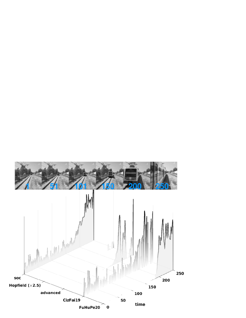
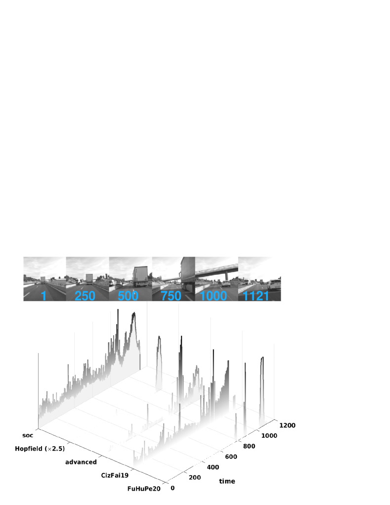
Figure 13 shows model responses to two videos without an actual or imminent collisions. Therefore, all models should ideally stay silent. The first video shows a train that seems to be on a collision course, but ultimately drives past the viewer. Because the camera was handheld, there is also a certain amount of camera shake which accounts for the non-zero SOC responses throughout. Camera shake translates to sudden wide/large-field movement which should be suppressed. In the locust visual system, LGMD responses to wide-field motion are suppressed by feedforward inhibition [41, 39]. From all models, “Hopfield” shows the smallest activity (note that “Hopfield”-responses were scaled by factor ). The rest of the models have a clear increase of activity in the final phase of the approach, where wide-field movement is suppressed in the output of “FuHuPe20” and “Advanced”, but not in “CizFai19”.
Figure 13b shows two typical situations that may occur when driving on a highway: first we overtake a truck and then we drive under a bridge. None of these events implies an imminent collision, therefore all model output should remain zero. The video involves complex background movement (e.g. oncoming vehicles, road marking, guard railings), as evidenced by the noisy SOC activity. SOC also reflects the overtaking maneuver from frame to . The first activity peak (frame ) is when the rear of the truck moves out of sight. The second peak (frame ) comes from the front of the truck as it moves out of the field of view. Finally, the last peak is produced by the bridge. The “Hopfield”-model in particular does not respond to these events, but shows a spurious peak around frame , just when the overtaking maneuver has been completed (recall that “Hopfield”-responses were scaled by ). It stays silent during the rest of the drive. The “FuHuPe20”-model shows narrow response peaks to all events: start and finish of overtaking and the bridge. “Advanced” shows a strong response to the end of the overtaking maneuver, and less to the bridge. There appears another narrow peak with low amplitude around frame , caused by an oncoming truck on the opposite lane. Finally. “CizFai19” responds to all events in an undifferentiated way.
4 Discussion and Conclusions
Summary. In this paper, I proposed a radically different algorithm for signaling object approaches which is based on modern Hopfield networks. It includes separated information processing along parallel ON- and OFF-channels. The critical mechanism that enables the use of Hopfield networks in the context of collision detection is a dynamic pattern memory. That is, at each time step, the memory is updated with a delayed video frame. Since Hopfield networks will always retrieve the pattern that best correlates with its initial state, the model would perform rather erratically without the memory update.
The proposed model is quite different from the bulk of published approaches, which extract temporal contrast from their input. SOC-based models are often biologically inspired, and model, for example, the neuronal circuitry of the LGMD neuron of the locust. To assess the performance of the “Hopfield”-model, its principal characteristics were studied with artificial video sequences. Subsequently, the output of three representative SOC-based models where compared with “Hopfield” for a couple of benchmark videos.
All of the considered SOC-based models are highpass filters in time, and their output is related to the angular velocity (cf. Figure 1). Conversely, since in the memory of the “Hopfield”-model a template pattern is stored with different sizes, its output is related to angular size. Furthermore, “Hopfield” involves spatial highpass filtering for processing the video frames and for its memory.
The results of the models can often be attributed to their different filtering characteristics (spatial vs. temporal highpass). For instance, SOC-based models will eventually fail to track an approaching object against a background grating with a high drifting frequency. “Hopfield”, on the other hand, will have a poor performance when the background grating matches the orientation of the template pattern (cf. Figure 3). In that sense, both model types are complementary and could be used in parallel in order to reduce the number of false collision alerts or missed approaches.
It is likely that the “Hopfield”-model could be made more robust by increasing the number of pattern memories for storing a variety of template pattern. This was not subject of the present work, since it has to be studied carefully how to combine the retrieval results across multiple pattern memories.
Dashcam footage and cropped video frames. In reference [17], dashcam videos with different traffic situations were shown to locusts and responses of the descending contralateral movement detector (DCMD) neuron were recorded. The DCMD replicates LGMD firing up to a frequency of Hz [38, 24]. It was found that the DCMD could distinguish traffic situations where collisions occur from normal driving. After challenging the “Hopfield”-model with dashcam footage extracted from Youtube crash compilations, I found that the “Hopfield”-model did not generate any response to videos showing all types of collisions (e.g., frontal and lateral) and near misses. The dashcam videos usually have a wide field of view and have much distortion which is typical of non-corrected lenses in short focal lengths. Furthermore, due to the aspect ratio, the footage typically occupied only one third of the frame when embedded in a square frame format. The Balloon Car Sequence of Figure 12a has similar properties, but a narrower field of view with few distortion. Furthermore, an uncropped version of the Balloon Car Sequence did not change the responses of “Hopfield”, nor did the “Hopfield”-model respond in a different way to a cropped version of the Train Sequence (Figure 13) with a wider field of view. This suggests that the field of view and the degree of distortion of the video is critical for a proper functioning of “Hopfield”.
Usage of stored patterns. The amplitude of “Hopfield”-responses reflects the retrieved pattern. Why does the model only use a limited range of the stored pattern vectors, but not continuously respond to the angular size of an approaching object? This is because of the dynamic memory update by a five time steps delayed video frame (Equation 5). For a “vanilla” object approach (uniform white disk approaching against a uniform black background, see Figure 1), the relationship between the delay and the response onset is such that the longer the delay, the earlier the response onset to the approaching disk. However, the advance of the response onset is only moderate, even for long delays (e.g. vs. time steps). This relationship does not readily generalize to real-world videos, where with different numbers of delay time steps the response curves of “Hopfield” may become noisier, response amplitudes may be altered, and finally the response onset may be advanced or even delayed. Furthermore, when an object that will eventually collide with the observer is still far, then it may not be exactly in the image center (e.g. due to camera shake). As consequence the tiny versions of the template pattern will not be retrieved. Therefore, for real-world videos one can expect lower hit-rates at bigger distances. Notice that distant objects will also generate few temporal contrast, leading to a comparable “problem” for SOC-based models as well.
Biological plausibility. In humans, (auto-) associative processes are thought to play an important role for perception, prediction and behavior [3]. For example, object recognition in the brain makes use of such content-addressable memories in order to organize bottom-up sensory input [2]. This makes the whole process quick and reliable, even when the sensory input is incomplete (e.g. occluded objects), ambiguous (e.g. few visual cues [54]) or has a poor resolution (e.g., face recognition from a large distance [7]). Therefore, at least for the human brain, “Hopfield” may represent a plausible model of how angular size is perceived. Note that when the extent of an object has been learned previously, then its exact absolute distance could be computed from measuring the angular size of its image projected on the retina. The pattern memory (Equation 5) may be implemented biologically with a different structure than a matrix.
To simplify notation, I refer to retinotopically arranged units such as photoreceptors and postsynaptic neurons (e.g. motion detectors [18]) as image for short. The pattern memory could be implemented with a dendritic processing scheme as follows. Synapses at the distal part of the dendrite would receive input from the central part of the image. The connectivity pattern would replicate the shape of the template pattern (Figure 3). Since the template patterns are sparse (because of spatial highpass filtering), connections would only be required along their contours. Synapses at the proximal part of the dendrite would receive input from the peripheral regions of the image. With this scheme, an approaching object would activate each time more proximal synapses as it moves closer to the observer. At the start of the approach, a postsynaptic potential (PSP) is generated at the distal site. This PSP package travels down the dendrite while the object is approaching further and keeps on with generating more PSPs along the dendrite. If the location of the synapses and the length of the dendrite is matched with the preferred speed and size of the approaching object, then previously generated PSPs (that travel downwards) coincide with currently generated ones. This would cause a continuous increase of the PSP amplitude during an approach. A suitable chosen threshold on the final PSP amplitude would therefore be tantamount to a threshold in angular size.
In fact, many animals and insects appear to trigger escape or avoidance reactions by a threshold in angular size [55]. The Fiddler crab seems to be an exception as it relies instead on a threshold in angular velocity [9].
Specifically, it has been hypothesized that locusts optimized their escape reactions to predators of diameters around to mm [40], and avoidance reactions in flight are triggered around degrees of visual angle [43]. Any such size preference must be encoded somewhere in the LGMD circuit, and the just outlined dendritic processing scheme could master that.
Functions like for explaining distance perception [15] or for fitting LGMD-responses [19] postulate the availability of angular size apart from angular velocity (i.e., SOC). So do theoretical accounts which address the biophysical implementations of and , respectively [13, 25, 27, 26]. Although non-retinotopic feedforward inhibition received by the LGMD seems to be related to [36, 44], no precise statement has been made as to its computation.
On the other hand, the majority of models for collision detection and avoidance start with computing the difference between successive image frames. As mentioned, summing the activity across a difference image is proportional to angular velocity in the absence of both background movement and weird lighting conditions. Mathematically, in order to recover angular size, one has to integrate successive measurements of angular velocity. Integration on-the-fly could be carried out by a dendritic processing scheme similar to the one sketched above. Another possibility to estimate angular size (given rate of expansion) is by suppressing all activity enclosed by the outer contour of an object’s projected image [28]. The idea therefore is to just keep the activity corresponding to the outer contour. In the case of a sphere, the outer contour is the circumference of a circle. Then, the mean activity across the image would be proportional to angular size.
Learning to avoid obstacles
Reinforcement learning (RL) lends itself to detect or avoid collisions: a reward could be issued upon successfully avoiding an obstacle. Otherwise a penalty is imposed. Usually, RL entails the stochastic exploration of a set of rules (policies) for achieving some goal or task. Model parameters are adjusted according to the reinforcement signal. Abstractly speaking, however, RL just optimizes model parameters. In this broader sense, RL could appear in different scenarios.
For example, in this paper combinations of eight model parameters were systematically explored. Subsequently, the parameter values were selected which achieved the best possible performance over a set of eight benchmark videos. The selection of model parameters according to some evaluation score (or fitness function) is also at the heart of genetic algorithms (GA; [35]). Genetic algorithms converge faster to a good solution compared to brute-force-parameter-parsing. However, there is no guarantee that a GA finds the best solution.
A GA with a population size was used in [59] to optimize six model parameters of a simple LGMD-model . The optimization criterion was to reduce the number of false alerts and false misses across a set of benchmark videos.
In robotics, obstacle avoidance is often combined with path selection and navigation methods. Specifically, deep reinforcement learning (DRL) allows to train a single neural network that uses video images as input and motion signals as output (end-to-end approaches). Hierarchized architectures were proposed as well, where sensory processing and navigation is separated. Since it is impossible to give a in-depth review on this rapidly evolving topic, I limit myself to highlight a couple of typical examples.
The approach proposed in [16] combined a chaotic neuronal network (the actor) with a regular neuronal network (the critic). The critic evaluates the actor’s performance and computes the reward signal for RL. Both the actor and the critic received a total of sensory signals which informed about locations of the obstacle and the target, respectively, and the distance to the walls. The output of the actor are motor commands for the robot (left / right). Although the environment and problem configuration was rather simple, the interesting aspect of the proposal lies in the generation of the stochastic movements of the agent. With usual RL techniques, external noise has to be applied to generate the random behavior which is rewarded or penalized. In [16], however, the external noise was replaced by the internal dynamics of the chaotic neuronal network. Thus, during the learning process, attractors may form according to the agent’s goal. The network therefore can be tuned to be more goal-directed or more exploratory.
The approach of [20] used an LGMD model from [45]. Rather than plain luminance. normalized image moments [23] were fed into the LGMD model. Image moments are less sensitive to camera noise and intensity variations, respectively. The output (one dimensional) of the LGMD model was fed into a deep neuronal network (DNN) along with the relative position to the target to which a micro unmanned aerial vehicle (UAV) should move. The DNN was trained with DRL where an explicit reward function was used. It outputs navigation commands for the micro UAV. The trained network navigates the UAV through complex environments and thus shows that the one-dimensional LGMD signal computed from monocular camera input is sufficient for successfully avoiding collisions. This is remarkable in the sense that no explicit depth information seems necessary.
The latter proposal stands in contrast to [57], which relied on estimating depth information. To this end, a generative adversarial network (GAN) was trained to predict depth maps from monocular camera images in ”simple, maze-like environments”. An end-to-end approach was taken (where several models were compared to each other), where the input were the camera images along with its predicted depth map. For training a laser range finder was employed in order to determine the reward signal that was computed with an explicit reward function. Despite of being a generative model, the depth predictions of the GAN will likely fail in complex and unconstrained environments.
In [60], a shallow network was trained to replicate the receptive field (RF) structure and response properties of Drosophila’s LPLC2 neurons [30]. Receptive fields (RFs) were represented as kernels ( network output), where two RF models were compared with each other: linear receptive field (LRI) units and rectified inhibition (RI) units, respectively. The input to the network was optical flow magnitude in four orthogonal directions. Training data consisted of four types of artificial motion pattern (“loom-and-hit”, “loom-and-miss”, “retreat”, “rotation”) and were labeled with their respective collision probability (one for “loom-and-hit”, zero for the rest). A total of trajectories were generated for training. The filter kernels were evenly distributed across visual space. Different networks were trained with a different number of kernels (). Individual filter responses were pooled to evaluate the overall performance for signaling collisions. By assuming circular and mirror-symmetric kernels, the number of trainable parameters was reduced to (LRF) and (RI), respectively. Three further kernel types were created by rotating the trained kernel by and degree. The kernels were arranged accordingly across visual space. The resulting kernels matched their biological counterparts in that their pooled response is sensitive to radially outward moving edges such as being generated during an object approach, but is inhibited by retreating objects. Apart from this outward solution, a trivial solution and an inward solution emerged as a result from several training sessions with different network initializations. In line with biological LPLC2 neurons [1] the pooled responses encode angular size, although the input corresponds to optical flow signals (i.e., directional angular velocity).
In summary, there are two conceivable scenarios for the use of deep reinforcement learning (DRL) to avoid collisions. First, one can train a DRL-architecture with the output of any proposed collision avoidance model (CAM for short) to predict from their output whether a collision is about to occur or not (e.g. similar to [20]). Alternatively, the DRL-architecture could be trained to output the probability of an imminent collision. The second scenario is an end-to-end approach, which uses video frames as input (e.g. analogous to [57]). The advantage of the first approach is that it is less computationally demanding than an end-to-end approach. It can be expected that a vision-based end-to-end approach that reliably works in unconstrained environments requires a huge amount of (labeled) training data.
In general, although the performance of deep learning (DL)-architectures is often spectacular, the energy demand for training should not be undervalued. For example, reference [51] estimated that the development of an DL-architecture up to publication standards typically requires the training of candidate models across six months, what amounts to more than kilotons of emissions. Even worse, training large models such as a transformers will generate about kilotons of . This should be compared to the relatively modest computational demand of most published CAMs for development and optimization. Moreover, by adjusting frame rate and/or frame size, all of the considered CAM models can run on current hardware in real-time. A further concern about current DL-architectures relates to reliability and predictability. It is well established that DL-applications reflect any bias inherent in the data which were used for training. With respect to generalization performance, the complexity (i.e. the very number of free model parameters) disallows any systematic analysis based on its final configuration (i.e., after training). Apart from providing only limited insights into the information processing chain of a trained network, rather unexpected failures were reported: for example, DL-architectures trained for traffic sign recognition (or the recognition of other objects) can easily be led astray by just applying small modifications to the original traffic signs (e.g. with a sticker or a marker) [50, 10, 52]. Suchlike modifications would not impair the performance of CAM models.
References
- [1] Jan M. Ache, Jason Polsky, Shada Alghailani, Ruchi Parekh, Patrick Breads, Martin Y. Peek, Davi D. Bock, Catherine R. von Reyn, and Gwyneth M. Card, Neural basis for looming size and velocity encoding in the drosophila giant fiber escape pathway, Current Biology 29 (2019), no. 6, 1073–1081.e4.
- [2] M. Bar, Visual objects in context, Nature Reviews Neuroscience 5 (2004), 617–629.
- [3] M. Bar, E. Aminoff, M. Mason, and M. Fenske, The units of thought, Hippocampus 17 (2007), no. 5, 420–428.
- [4] M. Blanchard, F.C. Rind, and F.M.J. Verschure, Collision avoidance using a model of locust LGMD neuron, Robotics and Autonomous Systems 30 (2000), 17–38.
- [5] G.A. Carpenter and S. Grossberg, Adaptation and transmitter gating in vertebrate photoreceptors, Journal of Theoretical Biology 1 (1981), 1–42.
- [6] P. Cizek and J. Faigl, Self-supervised learning of the biologically-inspired obstacle avoidance of hexapod walking robot, Bioinspiration & Biomimetics 14 (2019), no. 4, 046002.
- [7] D. Cox, E. Meyers, and P. Sinha, Contextually evoked object-specific responses in human visual cortex, Science 304 (2004), no. 5667, 115–117.
- [8] M. Demircigil, J. Heusel, M. Löwe, S. Upgang, and F. Vermet, On a model of associative memory with huge storage capacity, Journal of Statistical Physics 168 (2017), no. 2, 288–299.
- [9] C.G. Donohue, Z.M. Bagheri, J.C. Partridge, and J.M. Hemmi, Fiddler crabs are unique in timing their escape responses based on speed-dependent visual cues, Current Biololgy 32 (2022), no. 23, 5159–5164.e4.
- [10] Kevin Eykholt, Ivan Evtimov, Earlence Fernandes, Bo Li, Amir Rahmati, Chaowei Xiao, Atul Prakash, Tadayoshi Kohno, and Dawn Song, Robust physical-world attacks on deep learning visual classification, 2018 IEEE/CVF Conference on Computer Vision and Pattern Recognition, 2018, pp. 1625–1634.
- [11] Q. Fu, C. Hu, J. Peng, F.C. Rind, and S. Yue, A robust collision perception visual neural network with specific selectivity to darker objects, IEEE Transactions on Cybernetics 50 (2020), no. 12, 5074–5088.
- [12] Q. Fu, C. Hu, J. Peng, and S. Yue, Shaping the collision selectivity in a looming sensitive neuron model with parallel ON and OFF pathways and spike frequency adaptation, Neural Networks 106 (2018), 127–143.
- [13] F. Gabbiani, H.G. Krapp, C. Koch, and G. Laurent, Multiplicative computation in a visual neuron sensitive to looming, Nature 420 (2002), 320–324.
- [14] G. Gallego, T. Delbrück, G. Orchard, C. Bartolozzi, B. Taba, A. Censi, S. Leutenegger, A.J. Davison, J. Conradt, K. Daniilidis, and D. Scaramuzza, Event-based vision: A survey, IEEE Transactions on Pattern Analysis and Machine Intelligence 44 (2022), no. 1, 154–180.
- [15] J.J. Gibson, The Perception of the Visual World, Houghton Mifflin, Boston, 1950.
- [16] Yuki Goto and Katsunari Shibata, Influence of the chaotic property on reinforcement learning using a chaotic neural network, Neural Information Processing (Cham) (Derong Liu, Shengli Xie, Yuanqing Li, Dongbin Zhao, and El-Sayed M. El-Alfy, eds.), Springer International Publishing, 2017, pp. 759–767.
- [17] F.J. Harris, Simplified bionic solutions: A simple bio-inspired vehicle collision detection system, Bioinspiration & Biomimetics 12 (2017), no. 2, 026007.
- [18] B. Hassenstein and W. Reichardt, Systemtheoretische Analyse der Zeit-, Reihenfolgen- und Vorzeichenauswertung bei der Bewegungsperzeption des Rüsselkäfers Chlorophanus, Zeitschrift für Naturforschung B 11 (1956), no. 9-10, 513–524.
- [19] N. Hatsopoulos, F. Gabbiani, and G. Laurent, Elementary computation of object approach by a wide-field visual neuron, Science 270 (1995), 1000–1003.
- [20] Lei He, Nabil Aouf, James F. Whidborne, and Bifeng Song, Integrated moment-based LGMD and deep reinforcement learning for UAV obstacle avoidance, 2020 IEEE International Conference on Robotics and Automation (ICRA), 2020, pp. 7491–7497.
- [21] J.J. Hopfield, Neural networks and physical systems with emergent collective computational abilities, Proceedings of the National Academy of Sciences USA 79 (1982), no. 8, 2554–2558.
- [22] , Neurons with graded response have collective computational properties like those of two-state neurons, Proceedings of the National Academy of Sciences USA 81 (1984), no. 10, 3088–3092.
- [23] Ming-Kuei Hu, Visual pattern recognition by moment invariants, IRE Transactions on Information Theory 8 (1962), no. 2, 179–187.
- [24] S. Judge and F.C. Rind, The locust dcmd, a movement-detecting neurone tightly tuned to collision trajectories, Journal of Experimental Biology 200 (1997), no. 16, 2209–2216.
- [25] M.S. Keil, Emergence of multiplication in a biophysical model of a wide-field visual neuron for computing object approaches: Dynamics, peaks, & fits, Advances in Neural Information Processing Systems 24 (J. Shawe-Taylor, R.S. Zemel, P. Bartlett, F.C.N. Pereira, and K.Q. Weinberger, eds.), 2011, pp. 469–477.
- [26] , Dendritic pooling of noisy threshold processes can explain many properties of a collision-sensitive visual neuron, PLoS Computational Biology 11 (2015), no. 10, e1004479.
- [27] M.S. Keil and J. López-Moliner, Unifying time to contact estimation and collision avoidance across species, PLoS Computational Biology 8 (2012), no. 8, e1002625.
- [28] M.S. Keil, E. Roca-Morena, and A. Rodríguez-Vázquez, A neural model of the locust visual system for detection of object approaches with real-world scenes, Proceedings of the Fourth IASTED International Conference (Marbella, Spain), vol. 5119, 6-8 September 2004, pp. 340–345.
- [29] M.S. Keil and A. Rodríguez-Vázquez, Towards a computational approach for collision avoidance with real-world scenes, Proceedings of SPIE: Bioengineered and Bioinspired Systems (Maspalomas, Gran Canaria, Canary Islands, Spain) (A. Rodríguez-Vázquez, D. Abbot, and R. Carmona, eds.), vol. 5119, SPIE - The International Society for Optical Engineering, 19-21 May 2003, pp. 285–296.
- [30] N.C. Klapoetke, A. Nern, M.Y. Peek, E.M. Rogers, P. Breads, G.M. Rubin, M.B. Reiser, and G.M. Card, Ultra-selective looming detection from radial motion opponency, Nature 551 (2017), 237–241.
- [31] D. Krotov and J.J. Hopfield, Dense associative memory for pattern recognition, Advances in Neural Information Processing Systems 29 (2016), 1172–1180.
- [32] , Large associative memory problem in neurobiology and machine learning, arxiv.org 2008.06996 [q-bio.NC] (2020).
- [33] F. Lei, Z. Peng, M. Liu, J. Peng, V. Cutsuridis, and S. Yue, A robust visual system for looming cue detection against translating motion, IEEE Transactions on Neural Networks and Learning Systems 34 (2023), no. 11, 8362–8376.
- [34] G. Liñám, J. Cuadri, M.S. Keil, R. Stafford, and E. Roca, A bio-inspired collision detection algorithm for VLSI implementation, Proceedings of SPIE: Bioengineered and Bioinspired Systems II (Sevilla, Spain) (A. Rodríguez-Vázquez, E. Roca, and D. Abbot, eds.), SPIE - The International Society for Optical Engineering, 9-11 May 2005.
- [35] Melanie Mitchell, An introduction to genetic algorithms, MIT Press, Cambridge, MA, 1996.
- [36] J. Palka, An inhibitory process influencing visual responses in a fibre of the ventral nerve cord of locusts, Journal of Insect Physiology 13 (1967), no. 2, 235–248.
- [37] H. Ramsauer, B. Schäfl, J. Lehner, P. Seidl, M. Widrich, L. Gruber, M. Holzleitner, M. Pavlović, G. Kjetil Sandve, V. Greiff, D. Kreil, M. Kopp, G. Klambauer, J. Brandstetter, and S. Hochreiter, Hopfield networks is all you need, arxiv.org 2008.02217 [cs.NE] (2020).
- [38] F.C. Rind, A chemical synapse between two motion detecting neurones in the locust brain, Journal of Experimental Biology 110 (1984), 143–167.
- [39] F.C. Rind and D.I. Bramwell, Neural network based on the input organization of an identified neuron signaling implending collision, Journal of Neurophysiology 75 (1996), no. 3, 967–985.
- [40] F.C. Rind and D.R. Santer, Collision avoidance and a looming sensitive neuron: size matters but biggest is not necessarily best, Proceeding of the Royal Society of London B 271 (2004), S27–S29.
- [41] F.C. Rind and P.J. Simmons, Orthopteran DCMD neuron: a reevaluation of responses to moving objects. I. Selective responses to approaching objects, Journal of Neurophysiology 68 (1992), no. 5, 1654–1666.
- [42] , Local circuit for the computation of object approach by an identified visual neuron in the locust, The Journal of Comparative Neurology 395 (1998), 405–415.
- [43] R. M. Robertson and A. G. Johnson, Retinal image size triggers obstacle avoidance in flying locusts, Naturwissenschaften 80 (1993), 176–178.
- [44] C.H.F. Rowell, M. O’Shea, and J.L.D. Williams, The neuronal basis of a sensory analyser, the acridid movement detector system.IV.The preference for small field stimuli, Journal of Experimental Biology 68 (1977), 157–185.
- [45] Yue. S. and Rind. F.C., Collision detection in complex dynamic scenes using an LGMD-based visual neural network with feature enhancement, IEEE Transactions on Neural Networks 17 (2006), no. 3, 705–716.
- [46] H. Scharr, Optimal operators in digital image processing (Optimale Operatoren in der Digitalen Bildverarbeitung), Ph.D. thesis, University of Heidelberg (Germany), Combined Faculties for the Natural Sciences and for Mathematics, 2000.
- [47] G.R. Schlotterer, Response of the locust descending movement detector neuron to rapidly approaching and withdrawing visual stimuli, Canadian Journal of Zoology 55 (1977), 1372–1376.
- [48] P.J. Simmons and F.C. Rind, Orthopteran DCMD neuron: a reevaluation of responses to moving objects. II. Critical cues for detecting approaching objects, Journal of Neurophysiology 68 (1992), no. 5, 1667–1682.
- [49] , Responses to object approach by a wide field visual neurone the lgmd2 of the locust: characterization and image cues, Journal of Comparative Physiology 180 (1997), no. 3, 203–214.
- [50] Chawin Sitawarin, Arjun Nitin Bhagoji, Arsalan Mosenia, Mung Chiang, and Prateek Mittal, Darts: Deceiving autonomous cars with toxic signs, arXiv.org 1802.06430 [cs.CR] (2018).
- [51] Emma Strubell, Ananya Ganesh, and Andrew McCallum, Energy and policy considerations for deep learning in NLP, Proceedings of the 57th Annual Meeting of the Association for Computational Linguistics (Florence, Italy), Association for Computational Linguistics, July 2019, pp. 3645–3650.
- [52] Jiawei Su, Danilo Vasconcellos Vargas, and Kouichi Sakurai, One pixel attack for fooling deep neural networks, IEEE Transactions on Evolutionary Computation 23 (2019), no. 5, 828–841.
- [53] M.H. Tayarani-Najaran and M. Schmuker, Event-based sensing and signal processing in the visual, auditory, and olfactory domain: A review, Frontiers in Neural Circuits 31 (2021), no. 15, 610446.
- [54] C. Teufel, S.C. Dakin, and P.C. Fletcher, Prior object-knowledge sharpens properties of early visual feature-detectors, Scientific Reports 8 (2018), no. 1, 10853.
- [55] D. Tomsic and F.C. Rind, Animal behavior: Timing escape on angular size or angular velocity?, Current Biology 33 (2023), no. 3, R108–R110.
- [56] A. Vaswani, N. Shazeer, N. Parmar, J. Uszkoreit, L. Jones, A. N. Gomez, Ł. Kaiser, , and I. Polosukhin, Attention is all you need, Advances in Neural Information Processing Systems 30 (2017), 5998–6008.
- [57] Patrick Wenzel, Torsten Schön, Laura Leal-Taixé, and Daniel Cremers, Vision-based mobile robotics obstacle avoidance with deep reinforcement learning, 2021 IEEE International Conference on Robotics and Automation (ICRA), 2021, pp. 14360–14366.
- [58] M. Widrich, B. Schäfl, M. Pavlović, H. Ramsauer, L. Gruber, M. Holzleitner, J. Brandstetter, G. Kjetil Sandve, V. Greiff, S. Hochreiter, and G. Klambauer, Modern hopfield networks and attention for immune repertoire classification, Advances in Neural Information Processing Systems 33 (2020), 18832–18845.
- [59] S. Yue, F.C. Rind, M.S. Keil, J. Cuadri-Carvajo, and R. Stafford, A bio-inspired visual collision detection mechanism for cars: Optimisation of a model of a locust neuron to a novel environment, Neurocomputing 69 (2006), no. 13–15, 1591–1598.
- [60] Baohua Zhou, Zifan Li, Sunnie Kim, John Lafferty, and Damon A Clark, Shallow neural networks trained to detect collisions recover features of visual loom-selective neurons, eLife 11 (2022), e72067.