Analytic Formulas for the Anomalous Hall Effect in Itinerant Magnets

Abstract

We clarify the origin of what is sometimes called the “topological anomalous Hall effect,” provide analytical formulas to compute all the contributions to the Hall conductivity in the presence of Kondo-coupled spins and spin orbit coupling. The derivation is technical but we emphasize that the results can be very easily applied.

Introduction.—The electrical Hall effect, whereby a current transverse to an applied electric field can flow, proceeds from the coupling of a magnetic field to itinerant electrons. The (electrical) anomalous Hall effect Nagaosa (2006); Culcer (2024) refers to the same phenomenon when the Hall conductivity is not directly proportional to an applied magnetic field and, without skew scattering, generally arises from an electronic Berry curvature. Given the momentum-space Berry curvature for a band $n$ of (effectively) free electrons at each point in the Brillouin zone $\boldsymbol{k}$, $\Omega_{(n)}^{\gamma}(\boldsymbol{k})=i\epsilon_{\alpha\beta\gamma}\partial_{k_{\alpha}}[\langle u_{n}(\boldsymbol{k})|\partial_{k_{\beta}}u_{n}(\boldsymbol{k})\rangle]$, with $\alpha,\beta,\gamma$ cartesian coordinates, $|u_{n}(\boldsymbol{k})\rangle$ the unit cell periodic part of the single-electron wavefunction in band $n$, the TKNN formula provides the resulting electrical Hall conductivity, $\sigma^{xy}_{\rm H}=\sum_{n}\int_{\boldsymbol{k}}\Omega_{(n)}^{z}(\boldsymbol{k})f_{n}(\boldsymbol{k})$, where $f_{n}(\boldsymbol{k})$ is the electronic filling function of band $n$ at momentum $\boldsymbol{k}$. In turn, “sources” of Berry flux such as band crossings, e.g. in Weyl semimetals, will then naturally produce a nonzero Hall conductivity Burkov and Balents (2011). While the Berry curvature appearing in the Hall conductivity formula Karplus and Luttinger (1954); Adams and Blount (1959); Thouless et al. (1982) written above may be a characteristic of the pure (‘intrinsic’) electronic bands (we mean a band structure with spin-orbit coupling), it can also arise from a ‘reconstructed’ band structure resulting from the (‘extrinsic’) coupling of the charge carriers to other degrees of freedom. This is expected to be the case in particular when electrons couple to spins which locally (or globally) display nonzero spin chirality, $\chi_{ijk}=\vec{S}_{i}\cdot(\vec{S}_{j}\times\vec{S}_{k})$ for spins at three site $i,j,k$ or when the spin-orbit structure and a (possibly coplanar) spin structure conspire to produce a nonzero Berry curvature Ye et al. (1999); Chen et al. (2014); Zhang et al. (2020); Li et al. (2023). $\chi_{ijk}$ can be viewed as a ‘real space Berry curvature’ Zhang et al. (2020) and continuum versions such as $\vec{n}\cdot(\partial_{x_{\mu}}\vec{n}\times\partial_{x_{\nu}}\vec{n})$ appear in semiclassical (long-wavelength) approaches Wickles and Belzig (2013); Mangeolle et al. (2024). In practice the effects of both the structure of the pure electronic bands and that of the coupling to other degrees of freedom combine and couple. To the best of our knowledge, only within some approximations (e.g. double exchange Karplus and Luttinger (1954)) and under specific assumptions (e.g. long-wavelength limit) has the explicit relation between ‘real space Berry curvature’ and Hall conductivity been shown, and the effects of spin-orbit coupling have only been analyzed numerically.

Here, we derive analytical formulas for the Hall conductivity directly in terms of (i) real space structures such as spin chiralities within a unit cell and (ii) spin-orbit coupled hopping terms, and include all combinations of effects. To proceed, we make use of formulas for the Berry curvature and quantum metric in terms of projection operators, and expressions for the projectors as polynomials of the Hamiltonian matrix.

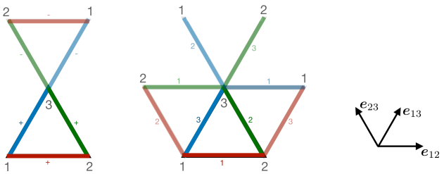
Figure 1: Three-sublattice cases: kagomé (left) and three-sublattice triangular (middle) lattices, with $\boldsymbol{e}_{12}^{(0)}=\boldsymbol{e}_{12}^{(1)}=(1,0)$, $\boldsymbol{e}_{23}^{(0)}=\boldsymbol{e}_{23}^{(2)}=\frac{1}{2}(-1,\sqrt{3})$, $\boldsymbol{e}_{31}^{(0)}=\boldsymbol{e}_{31}^{(3)}=\frac{-1}{2}(1,\sqrt{3})$.

Kondo-coupled band structure.—While the formalism developed here applies beyond this specific case, let us focus for concreteness on the case of a Kondo-coupled band structure with hamiltonian ${\rm H}=\frac{1}{\sqrt{N_{\rm u.c.}}}\sum_{\boldsymbol{k}}\Psi^{\dagger}_{\boldsymbol{k}}\hat{H}(\boldsymbol{k})\Psi^{\vphantom{\dagger}}_{\boldsymbol{k}}$ where $N_{\rm u.c.}$ is the number of unit cells, $\Psi^{\dagger}_{\boldsymbol{k}}$ is an $M=2N$ vector of spin-1/2 fermion creation operators, where $N$ is the number of sites in the (magnetic) unit cell, and $\hat{H}(\boldsymbol{k})$ is the following generic Hamiltonian matrix in reciprocal space:

$$\hat{H}(\boldsymbol{k}) =\sum_{a,b=1}^{N}\sum_{\mu=0}^{3}{\sf h}_{ab}^{\mu}({\boldsymbol{k}})\hat{E}_{ab}\hat{\sigma}^{\mu},$$ (1)

where $\hat{E}_{ab}$ is the $N\times N$ matrix with a $1$ at position $ab$ and zeros everywhere else, i.e. with matrix elements

$$(\hat{E}_{ab})_{ij}\equiv\delta_{ai}\delta_{bj},$$ (2)

where we use a ‘hat’ on $\hat{E}$ in order to emphasize $\hat{E}_{ab}$ is a matrix rather than a matrix element, $\hat{\sigma}^{0}={\rm Id}_{2}$ is the identity matrix, $\hat{\sigma}^{1,2,3}$ are the three Pauli matrices, with

$${\sf h}_{a\neq b}^{\mu}(\boldsymbol{k}) =\sum_{\eta=1}^{{\rm n}_{ab}}t_{ab,(\eta)}^{\mu}e^{i\boldsymbol{k}\cdot\boldsymbol{e}_{ab}^{(\eta)}},$$ (3)

$${\sf h}_{aa}^{\mu\neq 0}(\boldsymbol{k}) =K_{a}^{\mu}S_{a}^{\mu}+\sum_{\eta=1}^{{\rm n}_{aa}}t_{aa,(\eta)}^{\mu}e^{i\boldsymbol{k}\cdot\boldsymbol{e}_{aa}^{(\eta)}},$$

$${\sf h}_{aa}^{0}(\boldsymbol{k}) =\sum_{\eta=1}^{{\rm n}_{aa}}t_{aa,(\eta)}^{\mu}e^{i\boldsymbol{k}\cdot\boldsymbol{e}_{aa}^{(\eta)}},$$

where $ab$ is a bond between sublattices $a$ and $b$ and the sum over $\eta$ runs over the ${\rm n}_{ab}$ $ab$-type bonds with a nonzero hopping and separated by $\boldsymbol{e}_{a\neq b}^{(\eta)}=-\boldsymbol{e}_{ba}^{(\eta)}$, $K_{a}^{\mu}$ parametrizes the Kondo coupling on sublattice $a$, and hermiticity imposes $({\sf h}_{ab}^{\mu})^{*}={\sf h}_{ba}^{\mu}$ so that we can set $(t_{ab,(\eta)}^{\mu})^{*}=t_{ba,(\eta)}^{\mu}$ (more precisely, it is possible to make such choices of $\eta$). For convenience, we also define ${\sf h}_{ab,(\eta)}^{\mu}(\boldsymbol{k})$ such that ${\sf h}_{ab}^{\mu}(\boldsymbol{k})=\sum_{\eta}{\sf h}_{ab,(\eta)}^{\mu}(\boldsymbol{k})$, i.e. ${\sf h}_{ab,(\eta)}^{\mu}(\boldsymbol{k})=t_{ab,(\eta)}^{\mu}e^{i\boldsymbol{k}\cdot\boldsymbol{e}_{ab}^{(\eta)}}$ for $\eta=1,..,{\rm n}_{ab}$, and ${\sf h}_{aa,(0)}^{\mu\neq 0}(\boldsymbol{k})=K_{a}^{\mu}S_{a}^{\mu}$. We also note

$$\partial_{k_{\alpha}}{\sf h}_{ab}^{\mu}=i\sum_{\eta}e^{\alpha}_{ab,(\eta)}t_{ab,(\eta)}^{\mu}e^{i\boldsymbol{k}\cdot\boldsymbol{e}_{ab}^{(\eta)}}$$ (4)

for future reference. Note that it is the decomposition Eq. (1) in sublattice $a,b$ and spin $\mu$ indices and the separate traces which will allow to relate the Berry curvature to real space (sublattice) and spin quantities.

As applications, we will consider the nearest-neighbor kagomé lattice and the three-sublattice nearest-neighbor triangular lattice with a triangular basis, see Fig. 1. In both cases, $M=2N=6$. In the kagomé lattice case, on each $ab=12,23,31$-type bond, $\eta=1,2=\mp$. In the triangular lattice case, $\eta=1,2,3$ for each $ab$-bond type.

Formulas for the Berry curvature in terms of the Hamiltonian.—We now turn to the expressions of the Berry curvature and quantum metric in terms of the Hamiltonian. As mentioned above, we make use of band projectors in expressing the Berry curvature, and in particular rederive formulas present in Refs. Graf and Piéchon (2021); Graf (2022) using matrices rather than Bloch vectors. Using the formula $G_{(n)}^{\alpha\beta}={\rm Tr}[\partial_{\alpha}\hat{P}_{(n)}(1-\hat{P}_{(n)})\partial_{\beta}\hat{P}_{(n)}]$ for the quantum geometric tensor in band $n$ with “directions” $\alpha,\beta$ where $\partial_{\alpha}\equiv\partial_{k_{\alpha}}$, and $\hat{P}_{(n)}=|u_{n}(\boldsymbol{k})\rangle\langle u_{n}(\boldsymbol{k})|$ the projector into band $n$ (we will look only away from band degeneracies), we can write $G_{(n)}^{\alpha\beta}=\Gamma^{\alpha\beta}_{(n)}-\frac{i}{2}\Omega^{\alpha\beta}_{(n)}$ Provost and Vallée (1980); Resta (2011); Graf and Piéchon (2021), where $\Gamma^{\alpha\beta}_{(n)}\equiv{\rm Re}G_{(n)}^{\alpha\beta}$ and $\Omega^{\alpha\beta}_{(n)}=-2{\rm Im}G_{(n)}^{\alpha\beta}$ are the quantum metric Provost and Vallée (1980) and Berry curvature (note that in three-dimensions we can use equivalently two indices $\alpha\beta$ or one perpendicular direction index $\gamma$), respectively.

Then, using $\hat{H}=\sum_{n}\varepsilon_{n}\hat{P}_{(n)}$ ($\varepsilon_{n}$ is the energy in band $n$) and $\hat{P}_{(n)}=\prod_{m\neq n}(\hat{H}-\varepsilon_{m})/\prod_{m\neq n}(\varepsilon_{n}-\varepsilon_{m})$ one can show that

$$\hat{P}_{(n)}=\sum_{r=0}^{M-1}\ell^{(n)}_{r}\hat{H}^{r},$$ (5)

where $\ell^{(n)}_{r}$ are prefactors which depend only on $\varepsilon_{n}$ and ${\rm Tr}\hat{H}^{r^{\prime}}$, and $\hat{H}^{0}\equiv{\rm Id}_{M}$. The exact expressions of the prefactors $\ell_{r}^{(n)}$ are given in Appendix A.2 (Eq. (29)). What is most important is that (i) the sum in Eq. (5) terminates and (ii) $\hat{P}_{(n)}$ can be entirely expressed in terms of $\varepsilon_{n}(\boldsymbol{k})$ and the hamiltonian matrix $\hat{H}(\boldsymbol{k})$, i.e. in particular no eigenvectors are required and only the $n$th eigenvalue of $\hat{H}$ must be calculated. The finiteness of the sum in $\hat{P}_{(n)}$ means we can organize the terms in “powers” of $\hat{H}$, from $3$ to $3(M-1)$ in the case of the Berry curvature and from $2$ to $3(M-1)$ in the case of the quantum metric. The maximum number of matrix elements in a product therefore grows like the volume of the unit cell.

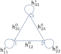
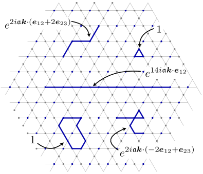
Figure 2: (a) Graphical representation of a length-6 loop (e.g. $r_{1}=r_{2}=r_{3}=2$) in a three-sublattice unit cell. This produces, among others a $\Lambda_{\{1,3\}}$ contribution (see Eqs. (7,E). (b) Loops of unit cell indices become strings on the lattice, with both start and end points belonging to the same sublattice. Here we are not showing on-site loops as in (a), but each site may host any number. In $\Omega^{\alpha\beta}_{(n)}$, each string is weighed by the factor shown multiplied by $e^{\alpha}_{a_{1}a_{2}(\eta_{1})}e^{\beta}_{a_{p}a_{p+1}(\eta_{p})}$ and any on-site factors. The straight line represents the contribution with the maximum possible extent.

Moreover, as noted in Refs. Graf and Piéchon (2021); Graf (2022), in the case of the Berry curvature, “orthogonality” relations (see Appendix B) allow one to rewrite the Berry curvature as

$$\Omega_{(n)}^{\alpha\beta} =-i\sum_{r_{1},r_{2},r_{3}}\ell^{(n)}_{r_{1}}\ell^{(n)}_{r_{2}}\ell^{(n)}_{r_{3}}{\rm Tr}\left[[\partial_{\beta}(\hat{H}^{r_{3}}),\partial_{\alpha}(\hat{H}^{r_{1}})]\hat{H}^{r_{2}}\right]$$ (6)

(the sums over the $r_{i}$ run from $1$ to $2N-1$), i.e. when applying the chain rule on $\partial_{\alpha/\beta}\hat{P}_{(n)}$ using Eq. (5) in $\Omega^{\alpha\beta}_{(n)}$, only the terms with the derivatives acting on the $\hat{H}^{r}$ survive, and not those with derivatives acting on the coefficients $\ell^{(n)}_{r}$. Furthermore, using the chain rule on Eq. (6), we can write, using $\sum_{p_{1}=0}^{r_{1}-1}\sum_{p_{3}=0}^{r_{3}-1}\cdots\sim\sum_{p=0}^{r_{1}+r_{3}-2}\xi_{r_{1},r_{3}}(p)\cdots$ with $\xi_{\{r_{i}\}}(p)={\rm min}\left[{\rm min}(r_{1},r_{3}),(r_{1}+r_{3})/2-|p-(R+r_{2}+2)/2|\right]\in\mathbb{N}$ when $\cdots$ depends on $p_{1}+p_{3}$ only,

$$\Omega^{\alpha\beta}_{(n)} =2\sum_{r_{1,2,3}}\ell_{r_{1}}^{(n)}\ell_{r_{2}}^{(n)}\ell_{r_{3}}^{(n)}$$ (7)

$$\quad\qquad\sum_{p=r_{2}+2}^{R}\xi_{\{r_{i}\}}(p){\rm Im}{\rm Tr}[\partial_{\alpha}\hat{H}\hat{H}^{p-2}\partial_{\beta}\hat{H}\hat{H}^{R-p}],$$

where we defined $R\equiv r_{1}+r_{2}+r_{3}$, and in the sum we have $q_{1}\equiv p-2\in\llbracket r_{2}-1,r_{1}+r_{2}-2\rrbracket$ and $q_{2}\equiv R-p\in\llbracket r_{3},r_{1}+r_{3}-1\rrbracket$. Because of the antisymmetry of $\Omega^{\alpha\beta}_{(n)}$ under $\alpha\leftrightarrow\beta$, many terms in the sums in Eq. (7) cancel. This is in particular true because $\Lambda_{(q_{1},q_{2})}^{\alpha\beta}\equiv{\rm Tr}[\partial_{\alpha}\hat{H}\hat{H}^{q_{1}}\partial_{\beta}\hat{H}\hat{H}^{q_{2}}]=-\Lambda_{(q_{2},q_{1})}^{\alpha\beta}$, so that in $\Omega^{\alpha\beta}_{(n)}$, if $\Lambda_{(q_{1},q_{2})}^{\alpha\beta}$ and $\Lambda_{(q_{2},q_{1})}^{\alpha\beta}$ both appear with the same $\ell$ prefactors, they cancel against one another. In Eq. (E) we provide the resulting explicit expression for the Berry curvature of a three-sublattice system.

Formulas for the Berry curvature in terms of Hamiltonian matrix elements.—Let us now write powers of $\hat{H}$ using the matrix elements defined above. We have $\hat{E}_{ab}\hat{E}_{cd}=\delta_{bc}\hat{E}_{ad}$, $\hat{\sigma}^{\mu}\hat{\sigma}^{\nu}=\sum_{\rho=0}^{3}g_{\mu\nu\rho}\hat{\sigma}^{\rho}$, with $g_{\mu\nu\rho}=d_{\mu\nu\rho}+if_{\mu\nu\rho}$ where, for $\mu,\nu,\rho=0,..,3$,

$$d_{\mu\nu\rho} =\delta_{(\mu\nu}\delta_{\rho)0}-2\delta_{\mu 0}\delta_{\nu 0}\delta_{\rho 0},$$

$$f_{\mu\nu\rho} =\epsilon_{\mu\nu\rho}.$$ (8)

Here $\delta_{(\mu\nu}\delta_{\rho)0}\equiv\delta_{\mu\nu}\delta_{\rho 0}+\delta_{\rho\mu}\delta_{\nu}+\delta_{\nu\rho}\delta_{\mu 0}$ is the symmetrized sum and $\epsilon_{\mu\nu\rho}$ is the three-dimensional Levi-Civita tensor where implicitly $\epsilon_{\mu\nu\rho}=0$ if $\mu$, $\nu$ or $\rho$ is zero. In turn,

$$\hat{H}^{r}=\sum_{\{\mu_{i}\},\{\rho_{j}\}}g_{\mu_{1}\mu_{2}\rho_{2}}\cdots g_{\rho_{r-1}\mu_{r}\rho_{r}}\hat{\sf H}_{\mu_{1}}\cdots\hat{\sf H}_{\mu_{r}}\hat{\sigma}_{\rho_{r}},$$ (9)

where $\hat{\sf H}_{\mu}$ is the $N\times N$ matrix with matrix elements $(\hat{\sf H}_{\mu})_{ab}={\sf h}_{ab}^{\mu}$, and we have $(\hat{\sf H}_{\mu})^{\dagger}=\hat{\sf H}_{\mu}$. Finally (recall $R=r_{1}+r_{2}+r_{3}$),

$$\Omega_{(n)}^{\alpha\beta}=2\sum_{r_{1},r_{2},r_{3}=1}^{2N-1}\mathcal{L}_{r_{1},r_{2},r_{3}}^{(n)}\sum_{\{\mu_{i}\}_{i=1,..,R}}\!\!\!{\rm Im}\left(\mathcal{G}_{\mu_{1}\cdots\mu_{R}}\sum_{p=r_{2}+2}^{R}\xi_{\{r_{i}\}}(p)\mathcal{H}_{\mu_{1}\cdots\mu_{R}}^{[p]}\right).$$ (10)

Here, $\mathcal{L}^{(n)}_{r_{1},r_{2},r_{3}}=\ell_{r_{1}}^{(n)}\ell_{r_{2}}^{(n)}\ell_{r_{3}}^{(n)}$ is the product of projector prefactors defined in Eq. (5), $\mathcal{G}_{\mu_{1}\cdots\mu_{R}}={\rm Tr}[\hat{\sigma}_{\mu_{1}}\cdots\hat{\sigma}_{\mu_{R}}]=\frac{1}{2}\sum_{\{\rho_{i}\}_{i=1,..,R}}g_{\rho_{R}\mu_{1}\rho_{1}}\cdots g_{\rho_{R-1}\mu_{R}\rho_{R}}$ (see Appendix C.1) is the contraction of Lie algebra structure constants defined in Eq. (Analytic Formulas for the Anomalous Hall Effect in Itinerant Magnets) and can be tabulated once and for all. It is $\mathcal{G}$ which will entirely fix the “geometric” structure of the terms in the Berry curvature, i.e. determine which contributions such as $\vec{S}_{i}\cdot(\vec{S}_{j}\times\vec{S}_{k})$, $\vec{S}_{i}\cdot\vec{S}_{j}$, $\vec{t}_{ij}\cdot(\vec{t}_{kl}\times\vec{t}_{mq})$, $\vec{t}_{ij}\cdot(\vec{S}_{k}\times\vec{S}_{l})$ etc. appear in $\Omega$ (see below). Finally

$$\mathcal{H}_{\mu_{1}\cdots\mu_{R}}^{\alpha\beta,[p]} ={\rm Tr}[\partial_{\alpha}\hat{\sf H}_{\mu_{1}}\hat{\sf H}_{\mu_{2}}\cdots\partial_{\beta}\hat{\sf H}_{\mu_{p}}\hat{\sf H}_{\mu_{p+1}}\cdots\hat{\sf H}_{\mu_{R}}],$$ (11)

where $p$ labels the index where $\partial_{\beta}$ acts. For the kagomé and three-sublattice triangular lattices, $1\leq r_{i}\leq 5$, and so $3\leq R\leq 15$.

It is interesting to make the structure of the Berry curvature as a sum of “loops” (resp. strings with ends on identical sublattices) of varying lengths within the unit cell—Fig. 2(a)—(resp. on the lattice—Fig. 2(b)) more obvious. Using Eq. (3), we write

$$\mathcal{H}_{\mu_{1}\cdots\mu_{R}}^{\alpha\beta,[p]} =\!\!\!\!\sum_{\{a_{1},a_{2},a_{p},a_{p+1}\}}\!\!\!\!J_{a_{1},a_{2},a_{p},a_{p+1}}^{\alpha\beta|\mu_{1}\mu_{p}}(\hat{\sf H}_{\mu_{2}}\cdots\hat{\sf H}_{\mu_{p-1}})_{a_{2}a_{p}}(\hat{\sf H}_{\mu_{p+1}}\cdots\hat{\sf H}_{\mu_{R}})_{a_{p+1}a_{1}},$$ (12)

and we note $(\hat{\sf H}_{\mu_{2}}\cdots\hat{\sf H}_{\mu_{p-1}})_{a_{2}a_{p}}={\sf h}^{\mu_{2}}_{a_{2}a_{3}}\cdots{\sf h}^{\mu_{p-1}}_{a_{p-1}a_{p}}$, and

$$J_{a_{1},a_{2},a_{p},a_{p+1}}^{\alpha\beta|\mu_{1}\mu_{p}} =-\sum_{\eta_{1},\eta_{p}}e_{a_{1}a_{2}(\eta_{1})}^{\alpha}e_{a_{p}a_{p+1}(\eta_{p})}^{\beta}{\sf h}^{\mu_{1}}_{a_{1}a_{2},(\eta_{1})}{\sf h}^{\mu_{p}}_{a_{p}a_{p+1},(\eta_{p})}$$ (13)

are the products of the matrix elements for the terms on which $\partial_{\alpha,\beta}$ act. We may therefore write

$$\mathcal{H}_{\mu_{1}\cdots\mu_{R}}^{\alpha\beta,[p]} =-\sum_{\{a_{i}\}}\sum_{\eta_{1},\eta_{p}}[e_{a_{1}a_{2}(\eta_{1})}^{\alpha}e_{a_{p}a_{p+1}(\eta_{p})}^{\beta}]\;{\sf h}^{\mu_{1}}_{a_{1}a_{2},(\eta_{1})}{\sf h}^{\mu_{2}}_{a_{2}a_{3}}\cdots{\sf h}^{\mu_{p}}_{a_{p}a_{p+1},(\eta_{p})}{\sf h}^{\mu_{p+1}}_{a_{p+1}a_{p+2}}\cdots{\sf h}^{\mu_{R}}_{a_{R}a_{1}}$$

$$=-\sum_{\{a_{i}\}}\sum_{\{\eta_{i}\}}[e_{a_{1}a_{2}(\eta_{1})}^{\alpha}e_{a_{p}a_{p+1}(\eta_{p})}^{\beta}]\;t^{\mu_{1}}_{a_{1}a_{2}(\eta_{1})}t^{\mu_{2}}_{a_{2}a_{3}(\eta_{2})}\cdots t^{\mu_{R}}_{a_{R}a_{1}(\eta_{R})}e^{i\boldsymbol{k}\cdot({\boldsymbol{e}}_{a_{1}a_{2}(\eta_{1})}+{\boldsymbol{e}}_{a_{2}a_{3}(\eta_{2})}+\cdots+{\boldsymbol{e}}_{a_{R}a_{1}(\eta_{R})})}.$$ (14)

We also note that the second line of Eq. (Analytic Formulas for the Anomalous Hall Effect in Itinerant Magnets) involves sums of $e^{i\boldsymbol{k}\cdot\boldsymbol{\mathcal{S}}}$, where

$$\boldsymbol{\mathcal{S}}=\boldsymbol{e}_{a_{1}a_{2}(\eta_{1})}+\cdots+\boldsymbol{e}_{a_{R}a_{1}(\eta_{R})}.$$ (15)

Because the ‘strings’ $\boldsymbol{\mathcal{S}}$ always “start” and “end” on a given sublattice, $\boldsymbol{\mathcal{S}}$ is always a Bravais lattice vector, $\boldsymbol{\mathcal{S}}=\sum_{i=1}^{d}\sum_{n_{i}}n_{i}\boldsymbol{A}_{i}$, $n_{i}\in\mathbb{Z}$, where the $\boldsymbol{A}_{i}$ are elementary Bravais lattice vectors. For the kagomé lattice where the distance between two nearest-neighbor sites is $\mathfrak{a}$, we have for example $\boldsymbol{A}_{1}=2\mathfrak{a}\boldsymbol{e}_{12}$ and $\boldsymbol{A}_{2}=2\mathfrak{a}\boldsymbol{e}_{13}$. In turn, while the $e^{i\boldsymbol{k}\cdot\boldsymbol{\mathcal{S}}}$ terms take different prefactors, as $R$ becomes larger, the sums of these terms become increasingly peaked around the $\boldsymbol{k}$ values where $\boldsymbol{k}\cdot\boldsymbol{\mathcal{S}}=0\;[2\pi]$, i.e. at the reciprocal Bravais lattice vectors, $\boldsymbol{k}_{\rm peak}=\sum_{i=1}^{d}\sum_{x_{i}}x_{i}\boldsymbol{B}_{i}$, $x_{i}\in\mathbb{Z}$, with e.g. $\boldsymbol{B}_{1}=\frac{\pi}{\mathfrak{a}}\frac{\boldsymbol{e}_{13}\times\boldsymbol{\hat{z}}}{\boldsymbol{e}_{12}\cdot(\boldsymbol{e}_{13}\times\boldsymbol{\hat{z}})}$, $\boldsymbol{B}_{2}=\frac{\pi}{\mathfrak{a}}\frac{\boldsymbol{\hat{z}}\times\boldsymbol{e}_{12}}{\boldsymbol{e}_{12}\cdot(\boldsymbol{e}_{13}\times\boldsymbol{\hat{z}})}$ for the kagomé lattice.

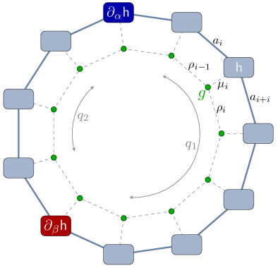
Figure 4: Graphical ‘tensor network’ representation of one of the terms in $\Omega_{(n)}^{\alpha\beta}$, Eq. (6), with $(q_{1},q_{2})=(6,3)$ present for example in the sum for $r_{1}=3$, $r_{2}=4$ and $r_{3}=4$. The light blue rectangles represent $\hat{\sf H}$ while the dark blue and dark red rectangles $\partial_{\alpha/\beta}\hat{\sf H}$, respectively, while the green circles represent the ‘structure constant’ $g=d+if$. Lines represent contractions of $\mu$ (between a rectangle and a circle) and $\rho$ (between circles) spin indices and $a$ site indices (between rectangles).

Finally, we note that $\Omega_{(n)}^{\alpha\beta}$ can be represented as a sum of contractions of tensors, which we show graphically in Fig. 4.

Nontrivial case where the Berry curvature vanishes for any spin configuration.—If (for $a\neq b$) ${\sf h}_{ab,(\eta)}^{\mu}=t_{0}e^{i\boldsymbol{k}\cdot\boldsymbol{e}_{ab(\eta)}}$ (i.e. $t_{ab(\eta)}^{\mu}$ is independent of $ab(\eta)$ and of $\mu$), then it is useful to define $\boldsymbol{I}_{ab}\equiv\sum_{\eta}\boldsymbol{e}_{ab(\eta)}e^{i\boldsymbol{k}\cdot\boldsymbol{e}_{ab(\eta)}}=-\boldsymbol{I}_{ba}^{*}$ (no summation over $a,b$!). In the case of the triangular lattice

$$\boldsymbol{I}_{ab}^{\rm t} =\upsilon_{ab}(\boldsymbol{e}_{12(0)}e^{i\upsilon_{ab}\boldsymbol{k}\cdot\boldsymbol{e}_{12(0)}}$$ (16)

$$\quad\qquad+\boldsymbol{e}_{23(0)}e^{i\upsilon_{ab}\boldsymbol{k}\cdot\boldsymbol{e}_{23(0)}}+\boldsymbol{e}_{31(0)}e^{i\upsilon_{ab}\boldsymbol{k}\cdot\boldsymbol{e}_{31(0)}}),$$

where $\upsilon_{12}=\upsilon_{23}=\upsilon_{31}$, $\upsilon_{ba}=-\upsilon_{ab}=\pm 1$. This entails that ${\boldsymbol{I}}_{12}^{\rm t}={\boldsymbol{I}}_{23}^{\rm t}={\boldsymbol{I}}_{31}^{\rm t}=-({\boldsymbol{I}}_{21}^{\rm t})^{*}=-({\boldsymbol{I}}_{32}^{\rm t})^{*}=-({\boldsymbol{I}}_{13}^{\rm t})^{*}$. Using the latter, the hermiticity of $\hat{\sf H}_{\mu}$, and $\Omega^{\alpha\beta}=-\Omega^{\beta\alpha}$ and $\Omega^{\alpha\beta}\in\mathbb{R}$, one can show that the Berry curvature vanishes for any configuration of the spins. This is an important result of this work. We provide details of the derivation in Appendix F. Note that this does not apply for example in the case of the kagomé lattice where $\boldsymbol{I}_{ab}^{\rm k}=\upsilon_{ab}\boldsymbol{e}_{ab}(e^{i\boldsymbol{k}\cdot\boldsymbol{e}_{ab}}-e^{-i\boldsymbol{k}\cdot\boldsymbol{e}_{ab}})^{\upsilon_{ab}}$ and so e.g. $\boldsymbol{I}_{12}^{\rm k}\neq\boldsymbol{I}_{23}^{\rm k}$.

Berry curvature as a “polynomial” of geometric elements of the spin (and/or hopping vector) texture in the unit cell.—We now investigate the structure of the contractions between $g$ tensors and $\hat{\sf H}_{\mu}$ matrices in order to explicitly express the Berry curvature as a “polynomial” in terms such as $\vec{S}_{i}\cdot\vec{S}_{j}$, $\vec{S}_{i}\cdot(\vec{S}_{j}\times\vec{S}_{k})$, and their products and powers, with $\boldsymbol{k}$-dependent coefficients that can be exactly and explicitly computed. [Note that we use quotation marks around “polynomial” because the $\ell_{r}^{(n)}$ coefficients also in principle depend on the spins through $\varepsilon_{n}$ and ${\rm Tr}\hat{H}^{r^{\prime}}$.] In other words, for three-sublattice systems without spin-orbit coupling, we can write:

$$\Omega^{\alpha\beta}_{(n)}(\mathbf{k})=\sum_{r_{1},r_{2},r_{3}}\ell^{(n)}_{r_{1}}\ell^{(n)}_{r_{2}}\ell^{(n)}_{r_{3}}\mathcal{P}^{\alpha\beta}_{i_{12},i_{23},i_{31},i_{123}}(\vec{S}_{1}\cdot\vec{S}_{2})^{i_{12}}(\vec{S}_{2}\cdot\vec{S}_{3})^{i_{23}}(\vec{S}_{3}\cdot\vec{S}_{1})^{i_{31}}(\chi_{123})^{i_{123}},$$ (17)

with $\chi_{123}=\vec{S}_{1}\cdot(\vec{S}_{2}\times\vec{S}_{3})$, $i_{12,23,31,123}\in\mathbb{N}$ and $i_{\rm tot}=2(i_{12}+i_{23}+i_{31})+3i_{123}\leq 13$, and the $\mathcal{P}$’s are functions of only $\boldsymbol{k}$ (and $t_{0},K$) that can be determined analytically. Importantly, in a spin-orbit coupling-free system, all contributions to the Berry curvature involve between $3$ and $3(2N-1)-2$ powers of $K$. Longer strings are only associated with higher $i_{\rm tot}$ and in turn higher powers of the Kondo coupling, so that in the weak-Kondo-coupling regime contributions from shorter strings will dominate the Berry curvature.

In the presence of spin-orbit coupling, one must include in the sum polynomials of all the following terms

$$(\vec{S}_{1}\cdot\vec{S}_{2}),(\vec{S}_{2}\cdot\vec{S}_{3}),(\vec{S}_{3}\cdot\vec{S}_{1})$$

$$(\chi_{123}),$$

$$(\vec{t}_{12}\cdot\vec{t}_{23}),(\vec{t}_{23}\cdot\vec{t}_{31}),(\vec{t}_{31}\cdot\vec{t}_{12})$$

$$(\vec{t}_{12}\cdot(\vec{t}_{23}\times\vec{t}_{31})),$$

$$(\vec{S}_{1}\cdot\vec{t}_{12}),(\vec{S}_{1}\cdot\vec{t}_{23}),(\vec{S}_{1}\cdot\vec{t}_{31}),(\vec{S}_{2}\cdot\vec{t}_{12}),(\vec{S}_{2}\cdot\vec{t}_{23}),(\vec{S}_{2}\cdot\vec{t}_{31}),(\vec{S}_{3}\cdot\vec{t}_{12}),(\vec{S}_{3}\cdot\vec{t}_{23}),(\vec{S}_{3}\cdot\vec{t}_{31}),$$

$$(\vec{t}_{12}\cdot(\vec{S}_{1}\times\vec{S}_{2})),(\vec{t}_{23}\cdot(\vec{S}_{1}\times\vec{S}_{2})),(\vec{t}_{31}\cdot(\vec{S}_{1}\times\vec{S}_{2})),(\vec{t}_{12}\cdot(\vec{S}_{2}\times\vec{S}_{3})),(\vec{t}_{23}\cdot(\vec{S}_{2}\times\vec{S}_{3})),(\vec{t}_{31}\cdot(\vec{S}_{2}\times\vec{S}_{3})),(\vec{t}_{12}\cdot(\vec{S}_{3}\times\vec{S}_{1})),$$

$$\qquad\qquad(\vec{t}_{23}\cdot(\vec{S}_{3}\times\vec{S}_{1})),(\vec{t}_{31}\cdot(\vec{S}_{3}\times\vec{S}_{1})),$$

$$(\vec{S}_{1}\cdot(\vec{t}_{12}\times\vec{t}_{23})),\cdots,$$ (18)

where $\vec{t}_{ab}\equiv(t^{x}_{ab},t^{y}_{ab},t^{z}_{ab})$ and we suppressed the $\eta$ subscripts for clarity (other “similar” combinations are also possible involving $(t_{ab}^{\mu})^{*}$ if the $t$’s are complex).

For (relative) simplicity, we focus on a nearest-neighbor-only case without spin-orbit coupling, $t^{0}_{a\neq b}=t_{0}$, $\vec{t}_{a\neq b}=\vec{0}$, $K_{a}^{\mu}=K$, and such that no nearest-neighbors belong to the same sublattice (this ensures that the terms on the diagonal blocks of the Hamiltonian matrix are Kondo-coupled spins only). Since $g_{\mu\nu 0}=\delta_{\mu\nu}$, in that case, the zero-components, $\mu=0$, correspond to intersublattice hopping terms (block off-diagonal, $a\neq b$), while the $\mu=1,2,3$ components are the Kondo-coupled spin terms (block diagonal, $a=b$). $\mathcal{H}$ comes down to summing the exponentials of all the paths one can take in a fixed (and bounded) number of (here, nearest-neighbor) steps from one sublattice point to another, see Fig. 2(b), and we find that $\Omega^{\alpha\beta}$ (away from band crossings) simply equals

$$\Omega^{\alpha\beta}_{(n)}(\boldsymbol{k})=\chi_{123}$$ (19)

$$\sum_{0\leq i_{12}+i_{23}+i_{31}\leq 2}\!\!\!\!\!\!\!\!\!\!\!\!\!\!\!w^{\alpha\beta}_{(n);i_{12},i_{23},i_{31}}(\boldsymbol{k})(\vec{S}_{1}\cdot\vec{S}_{2})^{i_{12}}(\vec{S}_{2}\cdot\vec{S}_{3})^{i_{23}}(\vec{S}_{3}\cdot\vec{S}_{1})^{i_{31}},$$

where the $w$’s are functions of $\boldsymbol{k}$, which we obtain analytically (we list the first few $\Lambda_{(q_{1},q_{2})}^{xy}$’s in Appendix E, Eq. (E)). In Figure 3 we plot $w^{xy}_{(n);000}$ for the kagomé lattice for $t_{0}=-1,K=1/2$ and $n=1$ (and $\vec{S}_{1}=(1,0,0)$, $\vec{S}_{2}=(0,1,0)$ and $\vec{S}_{3}=(0,0,1)$, whose specification is only required to compute $\epsilon_{n}(\boldsymbol{k})$ because it appears in the $\ell^{(n)}$’s).

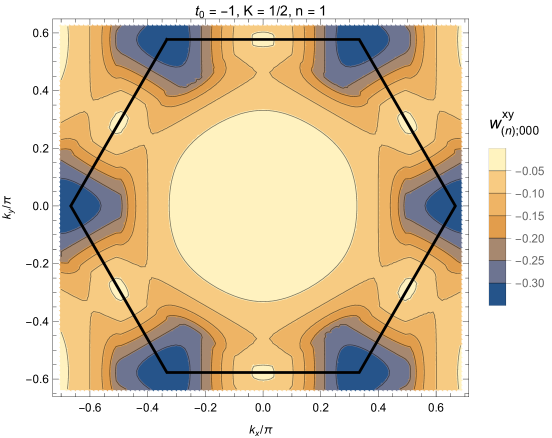
Figure 3: $w_{(1);000}^{xy}(\boldsymbol{k})$ as defined in Eq. (19), $\Omega_{(1)}^{xy}(\boldsymbol{k})=\chi_{123}w_{(1);000}^{xy}(\boldsymbol{k})$ with $\chi_{123}=\vec{S}_{1}\cdot(\vec{S}_{2}\times\vec{S}_{3})$, for the spin-orbit-coupling-free model on the kagomé lattice with $t_{0}=-1,K=1/2$ with $\vec{S}_{1}\perp\vec{S}_{2}\perp\vec{S}_{3}\perp\vec{S}_{1}$.

Discussion.—In this manuscript, we have provided an exact method to compute the Berry curvature analytically as a finite sum over finite strings on the lattice (this is in contrast, for example, with the claims in e.g. Ref. Tatara and Kawamura (2002)), in particular in electronic systems Kondo-coupled to spins. We made no assumptions on the strengh of the Kondo coupling, ‘double exchange’ Karplus and Luttinger (1954), long-wavelength limits, or on the size of the magnetic unit cell. We expect that this will allow a more accurate interpretation of experiments as well as easier and more accurate calculations of the Berry curvature and associated Hall conductivity than those accessible now Fukui et al. (2005); Weiße et al. (2006). Of course, beyond Berry curvature effects, skew-scattering Ishizuka and Nagaosa (2021); Nagaosa et al. (2010) may also contribute to $\sigma^{xy}_{\rm H}$ in real systems, but our exact derivation of the intrinsic effects should allow to better distinguish the contributions.

We explicitly applied our formalism to three-sublattice systems without spin-orbit coupling and showed that the Berry curvature vanished for the triangular lattice, regardless of the orientation of the spins. On the kagomé lattice (and any other three-sublattice system), we found that all contributions to the Berry curvature included a single power of the scalar chirality of the spins $\chi_{123}=\vec{S}_{1}\cdot(\vec{S}_{2}\times\vec{S}_{3})$ on one sublattice, and some of the ones involving higher powers of the Kondo coupling also included $\vec{S}_{i}\cdot\vec{S}_{j}$ elements.

This formalism allows for many extensions as it is merely an analytical way to relate energies and combinations of matrix elements to band quantities. In particular, higher-spin systems, systems with fluctuating spins, systems coupled to degrees of freedom other than spins, the computation of other observables Graf and Piéchon (2021), the quantum metric, and systems with any number of sublattices Diop et al. (2022); Martin and Batista (2008) can be studied the same way. In the latter case, we expect that quantities beyond three-sublattice chiralities and/or multiple powers of the spin-chiralities will appear because the imaginary part of traces of Pauli matrices can then involve, for example, additional Levi-Civita tensors. Taking the limit of the unit cell as the entire system (in a numerical experiment for example), where there will be both more allowed terms (“larger loops”), but also larger sums over small terms (“small loops”), we believe it might be possible to use the procedure presented in this manuscript as an expansion, perhaps in loop size, and truncate it.

As an even more immediate application, it will be interesting to explicitly explore the evolution of the Berry curvature as a function of spin-orbit coupling, the strength of the Kondo coupling and the size of the unit cell.

Appendix A Polynomials

Here we extend the results of Refs. Graf and Piéchon (2021); Graf (2022) to the case of traceful SU(M) basis matrices, and more specifically to the physical choice of basis we make (Eq. (17)).

A.1 Useful polynomial identities

Here we quote some well-known identities, also reviewed in Ref. Graf and Piéchon (2021); Graf (2022), useful for the derivations in Secs. A.2 and B.

The ‘elementary symmetric polynomials’ $\mathfrak{X}\mapsto\mathcal{E}_{r}(\mathfrak{X})$ with $r=0,..,|\mathfrak{X}|$ ($|\mathfrak{X}|$ denotes the size of the set $\mathfrak{X}$) are the sums of all distinct products of $r$ distinct variables taken from the set $\mathfrak{X}$, i.e.

$$\mathcal{E}_{0}(\{x_{1},\cdots,x_{M}\})=1,\qquad\mathcal{E}_{1}(\{x_{1},\cdots,x_{M}\})=\sum_{i=1}^{M}x_{i},$$

$$\mathcal{E}_{2}(\{x_{1},\cdots,x_{M}\})=\sum_{1\leq i<j\leq M}x_{i}x_{j},\qquad\cdots,$$

$$\mathcal{E}_{M}(\{x_{1},\cdots,x_{M}\})=\prod_{i=1}^{M}x_{i}.$$ (20)

The ‘complete exponential Bell polynomials’ $\mathfrak{X}\mapsto\mathcal{Y}_{r}(\mathfrak{X})$ with $r\in\mathbb{N}$ and $|\mathfrak{X}|=r$ are defined by

$$\mathcal{Y}_{0}(\{\})=1,\quad\mathcal{Y}_{r}(\{x_{1},\cdots,x_{r}\})=r!\sum\prod_{i=1}^{r}\frac{x_{i}^{j_{i}}}{(i!)^{j_{i}}j_{i}!},$$ (21)

where the sum is taken over the $\{j_{i}\in\mathbb{N}\}_{i=1,..,r}$ such that $\sum_{i=1}^{r}ij_{i}=r$ bel (2024).

Now we define the morphism of sets $\mathfrak{X}\mapsto\mathfrak{S}_{r}(\mathfrak{X})$

$$\mathfrak{S}_{0}(\mathfrak{X}) =\{\},$$ (22)

$$\mathfrak{S}_{r}(\{x_{1},..,x_{p}\}) =\left\{(-1)^{k-1}(k-1)!\left(\sum_{i=1}^{p}x_{i}^{k}\right)\right\}_{k=1,..,r}.$$

Note that $|\mathfrak{S}_{r}(\mathfrak{X})|=r$ independently of $|\mathfrak{X}|$. Newton’s identities allow to show that

$$\mathcal{E}_{r}(\mathfrak{X})=\frac{1}{r!}\mathcal{Y}_{r}(\mathfrak{S}_{r}(\mathfrak{X})).$$ (23)

These relations are particularly useful when expressing polynomials of the form:

$$\prod_{m=1}^{M}(x-x_{m})$$ (24)

$$=(-1)^{M}\prod_{m=1}^{M}x_{m}+\cdots-x^{M-1}\sum_{m=1}^{M}x_{m}+x^{M}$$

$$=\sum_{r=0}^{M}(-1)^{M-r}\mathcal{E}_{M-r}(\{x_{1},\cdots,x_{M}\})x^{r}$$

$$=\sum_{r=0}^{M}\frac{(-1)^{M-r}}{(M-r)!}\mathcal{Y}_{M-r}\Big{(}\mathfrak{S}_{M-r}(\{x_{1},\cdots,x_{M}\})\Big{)}x^{r}.$$

A.2 Projector as a polynomial in $H$

We have, in general, away from degeneracies, for $\{\varepsilon_{m}\}_{m=1,..,M}$ the eigenvalues of a $M\times M$ Hamiltonian $\hat{H}$, and $\hat{P}_{(n)}$ the projector onto the $n$th band of $\hat{H}$,

$$\hat{P}_{(n)}=\prod_{m\neq n}\frac{\hat{H}-\varepsilon_{m}}{\varepsilon_{n}-\varepsilon_{m}}=\frac{\prod_{m\neq n}(\hat{H}-\varepsilon_{m})}{\prod_{m\neq n}(\varepsilon_{n}-\varepsilon_{m})}.$$ (25)

If we expand the products in the numerator, we obtain

$$\prod_{m\neq n}(\hat{H}-\varepsilon_{m})$$ (26)

$$=\sum_{r=0}^{M-1}\frac{(-1)^{(M-1)-r}}{[(M-1)-r]!}\mathcal{Y}_{(M-1)-r}\Big{(}\mathfrak{S}_{(M-1)-r}^{(n)}(\hat{H})\Big{)}\hat{H}^{r},$$

where

$$\mathfrak{S}_{0}^{(n)}(\hat{H}) \equiv\{\},$$ (27)

$$\mathfrak{S}_{r>0}^{(n)}(\hat{H}) \equiv\mathfrak{S}_{r}(\{\varepsilon_{1},\cdots,\varepsilon_{n-1},\varepsilon_{n+1},\cdots,\varepsilon_{M}\})$$

$$=\left\{(-1)^{k-1}(k-1)!\left({\rm Tr}\hat{H}^{k}-\varepsilon_{n}^{k}\right)\right\}_{k=1,..,r}.$$

Similarly,

$$\prod_{m\neq n}(\varepsilon_{n}-\varepsilon_{m})$$

$$=\sum_{r=0}^{M-1}\frac{(-1)^{(M-1)-r}}{[(M-1)-r]!}\mathcal{Y}_{(M-1)-r}\Big{(}\mathfrak{S}_{(M-1)-r}^{(n)}(\hat{H})\Big{)}\varepsilon_{n}^{r},$$

$$\equiv\mathcal{N}_{(n)}(\hat{H})$$ (28)

and we define, for $r=0,..,M-1$,

$$\ell^{(n)}_{r}(\hat{H})\equiv\frac{(-1)^{(M-1)-r}}{[(M-1)-r]!}\frac{\mathcal{Y}_{(M-1)-r}\Big{(}\mathfrak{S}_{(M-1)-r}^{(n)}(\hat{H})\Big{)}}{\mathcal{N}_{(n)}(\hat{H})},$$ (29)

so that

$$\hat{P}_{(n)}=\sum_{r=0}^{M-1}\ell^{(n)}_{r}\hat{H}^{r},$$ (30)

as in the main text, Eq. (5).

A.3 Expressions for $M=6$

Here we give the expressions for $\mathcal{N}_{(n)}$ and $\ell_{r}^{(n)}$ defined in Eqs. (A.2,29) for a $6\times 6$ Hamiltonian. Defining, $\forall r\in\mathbb{N}$, $\mathcal{C}_{r}(\boldsymbol{k})\equiv{\rm Tr}\hat{H}^{r}(\boldsymbol{k})=\sum_{n=1}^{M}\varepsilon_{n}^{r}(\boldsymbol{k})$, i.e. the ‘$r$ power sum’ of the eigenvalues of $\hat{H}$ and

$$\mathcal{N}_{(n)} =6\varepsilon_{n}^{5}-5\mathcal{C}_{1}\varepsilon_{n}^{4}+2(\mathcal{C}_{1}^{2}-\mathcal{C}_{2})\varepsilon_{n}^{3}$$ (31)

$$\quad+\frac{1}{2}\left(-\mathcal{C}_{1}^{3}+3\mathcal{C}_{1}\mathcal{C}_{2}-2\mathcal{C}_{3}\right)\varepsilon_{n}^{2}$$

$$\quad+\frac{1}{12}\left(\mathcal{C}_{1}^{4}-6\mathcal{C}_{1}^{2}\mathcal{C}_{2}+3\mathcal{C}_{2}^{2}+8\mathcal{C}_{1}\mathcal{C}_{3}-6\mathcal{C}_{4}\right)\varepsilon_{n}$$

$$\quad+\frac{1}{120}\left(-\mathcal{C}_{1}^{5}+10\mathcal{C}_{1}^{3}\mathcal{C}_{2}-20\mathcal{C}_{1}^{2}\mathcal{C}_{3}+20\mathcal{C}_{2}\mathcal{C}_{3}\right.$$

$$\quad\qquad\qquad\left.-15\mathcal{C}_{1}(\mathcal{C}_{2}^{2}-2\mathcal{C}_{4})-24\mathcal{C}_{5}\right),$$

and

$$\mathcal{N}_{(n)}\ell_{0}^{(n)} =\varepsilon_{n}^{5}-\mathcal{C}_{1}\varepsilon_{n}^{4}+\frac{1}{2}(\mathcal{C}_{1}^{2}-\mathcal{C}_{2})\varepsilon_{n}^{3}$$

$$\quad+\frac{1}{6}(-\mathcal{C}_{1}^{3}+3\mathcal{C}_{1}\mathcal{C}_{2}-2\mathcal{C}_{3})\varepsilon_{n}^{2}$$

$$\quad+\frac{1}{24}(\mathcal{C}_{1}^{4}-6\mathcal{C}_{1}^{2}\mathcal{C}_{2}+3\mathcal{C}_{2}^{2}+8\mathcal{C}_{1}\mathcal{C}_{3}-6\mathcal{C}_{4})\varepsilon_{n}$$

$$\quad+\frac{1}{120}\left(-\mathcal{C}_{1}^{5}+10\mathcal{C}_{1}^{3}\mathcal{C}_{2}-20\mathcal{C}_{1}^{2}\mathcal{C}_{3}+20\mathcal{C}_{2}\mathcal{C}_{3}\right.$$

$$\quad\qquad\qquad\left.-15\mathcal{C}_{1}(\mathcal{C}_{2}^{2}-2\mathcal{C}_{4})-24\mathcal{C}_{5}\right),$$

$$\mathcal{N}_{(n)}\ell_{1}^{(n)} =\varepsilon_{n}^{4}-\mathcal{C}_{1}\varepsilon_{n}^{3}+\frac{1}{2}(\mathcal{C}_{1}^{2}-\mathcal{C}_{2})\varepsilon_{n}^{2}$$

$$\quad+\frac{1}{6}(-\mathcal{C}_{1}^{3}+3\mathcal{C}_{1}\mathcal{C}_{2}-2\mathcal{C}_{3})\varepsilon_{n}$$

$$\quad+\frac{1}{24}(\mathcal{C}_{1}^{4}-6\mathcal{C}_{1}^{2}\mathcal{C}_{2}+3\mathcal{C}_{2}^{2}+8\mathcal{C}_{1}\mathcal{C}_{3}-6\mathcal{C}_{4}),$$

$$\mathcal{N}_{(n)}\ell_{2}^{(n)} =\varepsilon_{n}^{3}-\mathcal{C}_{1}\varepsilon_{n}^{2}+\frac{1}{2}(\mathcal{C}_{1}^{2}-\mathcal{C}_{2})\varepsilon_{n}$$

$$\quad+\frac{1}{6}(-\mathcal{C}_{1}^{3}+3\mathcal{C}_{1}\mathcal{C}_{2}-2\mathcal{C}_{3}),$$

$$\mathcal{N}_{(n)}\ell_{3}^{(n)} =\varepsilon_{n}^{2}-\mathcal{C}_{1}\varepsilon_{n}+\frac{1}{2}(\mathcal{C}_{1}^{2}-\mathcal{C}_{2}),$$

$$\mathcal{N}_{(n)}\ell_{4}^{(n)} =\varepsilon_{n}-\mathcal{C}_{1},$$

$$\mathcal{N}_{(n)}\ell_{5}^{(n)} =1.$$ (32)

Appendix B Berry curvature in terms of powers of the Hamiltonian and eigenenergies

B.1 Expressions for the quantum geometric tensor

We start by recalling the definition of the quantum geometric tensor in terms of projection operators into bands Resta (2011); Graf and Piéchon (2021),

$$G_{(n)}^{\alpha\beta} ={\rm Tr}[\partial_{\alpha}\hat{P}_{(n)}(1-\hat{P}_{(n)})\partial_{\beta}\hat{P}_{(n)}].$$ (33)

Its symmetric part under $\alpha\leftrightarrow\beta$ is the quantum metric

$$\Gamma^{\alpha\beta}_{(n)} =\frac{1}{2}(G_{(n)}^{\alpha\beta}+G_{(n)}^{\beta\alpha})$$

$$={\rm Tr}[\partial_{\alpha}\hat{P}_{(n)}\partial_{\beta}\hat{P}_{(n)}]-\frac{1}{2}{\rm Tr}[\{\partial_{\beta}\hat{P}_{(n)},\partial_{\alpha}\hat{P}_{(n)}\}\hat{P}_{(n)}]$$

$$=\frac{1}{2}(G_{(n)}^{\alpha\beta}+[G_{(n)}^{\alpha\beta}]^{*})$$

$$={\rm Re}G^{\alpha\beta}_{(n)},$$ (34)

and the Berry curvature is

$$\Omega^{\alpha\beta}_{(n)} =i(G_{(n)}^{\alpha\beta}-G_{(n)}^{\beta\alpha})$$

$$=-i{\rm Tr}[[\partial_{\beta}\hat{P}_{(n)},\partial_{\alpha}\hat{P}_{(n)}]\hat{P}_{(n)}]$$

$$={\rm Im}\left({\rm Tr}[[\partial_{\beta}\hat{P}_{(n)},\partial_{\alpha}\hat{P}_{(n)}]\hat{P}_{(n)}]\right)$$

$$=i(G_{(n)}^{\alpha\beta}-[G_{(n)}^{\alpha\beta}]^{*})$$

$$=-2{\rm Im}G^{\alpha\beta}_{(n)}$$

$$=2{\rm Im}{\rm Tr}[\partial_{\alpha}\hat{P}_{(n)}\hat{P}_{(n)}\partial_{\beta}\hat{P}_{(n)}],$$ (35)

since ${\rm Im}{\rm Tr}[\partial_{\alpha}\hat{P}_{(n)}\partial_{\beta}\hat{P}_{(n)}]=0$.

In the more conventional form of eigenvectors,

$$G_{(n)}^{\alpha\beta} =\langle\partial_{\alpha}\psi_{n}|(1-\hat{P}_{(n)})|\partial_{\beta}\psi_{n}\rangle$$

$$=\sum_{m\neq n}\frac{\langle\psi_{n}|\partial_{\alpha}\hat{H}|\psi_{m}\rangle\langle\psi_{m}|\partial_{\beta}\hat{H}|\psi_{n}\rangle}{[\varepsilon_{n}-\varepsilon_{m}]^{2}},$$ (36)

and

$$\Gamma^{\alpha\beta}_{(n)}={\rm Re}\langle\partial_{\alpha}\psi_{n}|(1-\hat{P}_{(n)})|\partial_{\beta}\psi_{n}\rangle,$$ (37)

$$\Omega^{\alpha\beta}_{(n)} =-2{\rm Im}\langle\partial_{\alpha}\psi_{n}|(1-\hat{P}_{(n)})|\partial_{\beta}\psi_{n}\rangle$$

$$=-2{\rm Im}\langle\partial_{\alpha}\psi_{n}|\partial_{\beta}\psi_{n}\rangle$$

$$=i(\partial_{\alpha}[\langle\psi_{n}|\partial_{\beta}\psi_{n}\rangle]-\partial_{\beta}[\langle\psi_{n}|\partial_{\alpha}\psi_{n}\rangle]).$$ (38)

B.2 In terms of powers of the Hamiltonian and eigenenergies

In turn, using Eq. (30),

$$\Omega^{\alpha\beta}_{(n)} =2\sum_{r_{1},r_{2},r_{3}=0}^{M-1}{\rm Im}{\rm Tr}\left[\partial_{\alpha}[\ell_{r_{1}}^{(n)}\hat{H}^{r_{1}}]\ell_{r_{2}}^{(n)}\hat{H}^{r_{2}}\partial_{\beta}[\ell_{r_{3}}^{(n)}\hat{H}^{r_{3}}]\right],$$

$$\Gamma_{(n)}^{\alpha\beta} =\sum_{r_{1},r_{2}=0}^{M-1}{\rm Tr}\left[\partial_{\alpha}[\ell_{r_{1}}^{(n)}\hat{H}^{r_{1}}]\partial_{\beta}[\ell_{r_{2}}^{(n)}\hat{H}^{r_{2}}]\right]-\sum_{r_{1},r_{2},r_{3}=0}^{M-1}{\rm Re}{\rm Tr}\left[\partial_{\alpha}[\ell_{r_{1}}^{(n)}\hat{H}^{r_{1}}]\ell_{r_{2}}^{(n)}\hat{H}^{r_{2}}\partial_{\beta}[\ell_{r_{3}}^{(n)}\hat{H}^{r_{3}}]\right].$$ (39)

Note that this in principle requires to differentiate the $\ell$’s. However, as noted in Ref. Graf and Piéchon (2021); Graf (2022), an important simplification arises in the case of the Berry curvature, which we now examine. Using the chain rule, we have

$$\Omega^{\alpha\beta}_{(n)} =2\sum_{r_{1},r_{2},r_{3}=0}^{M-1}\ell_{r_{1}}^{(n)}\ell_{r_{2}}^{(n)}\ell_{r_{3}}^{(n)}{\rm Im}{\rm Tr}\left[\partial_{\alpha}[\hat{H}^{r_{1}}]\hat{H}^{r_{2}}\partial_{\beta}[\hat{H}^{r_{3}}]\right]+2\sum_{r_{1},r_{2},r_{3}=0}^{M-1}\partial_{\alpha}\ell_{r_{1}}^{(n)}\ell_{r_{2}}^{(n)}\partial_{\beta}\ell_{r_{3}}^{(n)}{\rm Im}{\rm Tr}\left[\hat{H}^{r_{1}}\hat{H}^{r_{2}}\hat{H}^{r_{3}}\right]$$

$$\quad+2\sum_{r_{1},r_{2},r_{3}=0}^{M-1}\ell_{r_{1}}^{(n)}\ell_{r_{2}}^{(n)}\partial_{\beta}\ell_{r_{3}}^{(n)}{\rm Im}{\rm Tr}\left[\partial_{\alpha}[\hat{H}^{r_{1}}]\hat{H}^{r_{2}}\hat{H}^{r_{3}}\right]+2\sum_{r_{1},r_{2},r_{3}=0}^{M-1}\partial_{\alpha}\ell_{r_{1}}^{(n)}\ell_{r_{2}}^{(n)}\ell_{r_{3}}^{(n)}{\rm Im}{\rm Tr}\left[\hat{H}^{r_{1}}\hat{H}^{r_{2}}\partial_{\beta}[\hat{H}^{r_{3}}]\right].$$ (40)

Using the antisymmetry of $\Omega^{\alpha\beta}_{(n)}$ under the $\alpha\leftrightarrow\beta$ exchange, i.e. $\Omega^{\beta\alpha}_{(n)}=-\Omega^{\alpha\beta}_{(n)}$, we now show that only the first term of Eq. (B.2) survives. Indeed, relabeling the dummy indices $r_{1}\leftrightarrow r_{3}$ in half the terms, we find

$$\frac{1}{2}(\Omega^{\alpha\beta}_{(n)}-\Omega^{\beta\alpha}_{(n)}) =\sum_{r_{1},r_{2},r_{3}=0}^{M-1}\ell_{r_{1}}^{(n)}\ell_{r_{2}}^{(n)}\ell_{r_{3}}^{(n)}{\rm Im}{\rm Tr}\left[[\partial_{\beta}[\hat{H}^{r_{3}}],\partial_{\alpha}[\hat{H}^{r_{1}}]]\hat{H}^{r_{2}}\right]+\sum_{r_{1},r_{2},r_{3}=0}^{M-1}\partial_{\alpha}\ell_{r_{1}}^{(n)}\ell_{r_{2}}^{(n)}\partial_{\beta}\ell_{r_{3}}^{(n)}{\rm Im}{\rm Tr}\left[[\hat{H}^{r_{3}},\hat{H}^{r_{1}}]\hat{H}^{r_{2}}\right]$$

$$\quad+\sum_{r_{1},r_{2},r_{3}=0}^{M-1}\ell_{r_{1}}^{(n)}\ell_{r_{2}}^{(n)}\partial_{\beta}\ell_{r_{3}}^{(n)}{\rm Im}{\rm Tr}\left[\partial_{\alpha}[\hat{H}^{r_{1}}][\hat{H}^{r_{2}},\hat{H}^{r_{3}}]\right]+\sum_{r_{1},r_{2},r_{3}=0}^{M-1}\partial_{\alpha}\ell_{r_{1}}^{(n)}\ell_{r_{2}}^{(n)}\ell_{r_{3}}^{(n)}{\rm Im}{\rm Tr}\left[[\hat{H}^{r_{1}},\hat{H}^{r_{2}}]\partial_{\beta}[\hat{H}^{r_{3}}]\right].$$ (41)

Since $[\hat{H}^{r},\hat{H}^{r^{\prime}}]=0$, we have

$$\Omega^{\alpha\beta}_{(n)} =2\sum_{r_{1},r_{2},r_{3}=1}^{M-1}\ell^{(n)}_{r_{1}}\ell_{r_{2}}^{(n)}\ell_{r_{3}}^{(n)}{\rm Im}{\rm Tr}\left[\partial_{\alpha}[\hat{H}^{r_{1}}]\hat{H}^{r_{2}}\partial_{\beta}[\hat{H}^{r_{3}}]\right],$$ (42)

where we removed the $r_{i}=0$ terms in the sum since they identically vanish. Indeed, $\hat{H}^{0}\equiv{\rm Id}_{M}$ has only constant elements, so its derivative vanishes. Moreover, note that we can rewrite the $r_{2}=0$ contribution as $\partial_{\alpha}[\hat{H}^{r_{1}}]\hat{H}^{0}\partial_{\beta}[\hat{H}^{r_{3}}]$ whose sum over $r_{1},r_{3}$ in $\Omega^{\alpha\beta}$ vanishes since it is symmetric under $\alpha\leftrightarrow\beta$ while $\Omega^{\alpha\beta}$ is antisymmetric under this exchange.

Appendix C Explicit contractions in spin space

C.1 General relations

In sublattice space,

$$\hat{E}_{a_{1}a_{2}}\hat{E}_{a_{3}a_{4}}\cdots\hat{E}_{a_{2r-1}a_{2r}}=\delta_{a_{2}a_{3}}\delta_{a_{4}a_{5}}\cdots\delta_{a_{2r-2}a_{2r-1}}\hat{E}_{a_{1}a_{2r}}$$ (43)

and, in spin space, for $r\geq 2$,

$$\hat{\sigma}_{\mu_{1}}\hat{\sigma}_{\mu_{2}}\cdots\hat{\sigma}_{\mu_{r}}=\sum_{\{\rho_{i}\}_{i=2,..,r}}\!\!\!\!g_{\mu_{1}\mu_{2}\rho_{2}}g_{\rho_{2}\mu_{3}\rho_{3}}\cdots g_{\rho_{r-1}\mu_{r}\rho_{r}}\hat{\sigma}_{\rho_{r}}.$$ (44)

We have for $\mu,\nu,\rho=0,1,2,3$, $\zeta=\pm 1$ and $[\hat{A},\hat{B}]_{\zeta}=\hat{A}\hat{B}+\zeta\hat{B}\hat{A}$ for two matrices $\hat{A}$ and $\hat{B}$:

$${\rm Tr}\left([\hat{\sigma}^{\mu},\hat{\sigma}^{\nu}]_{\zeta}\hat{\sigma}^{\rho}\right)$$ (45)

$$=4i\frac{(1-\zeta)}{2}\epsilon_{\mu\nu\rho}+4\frac{(1+\zeta)}{2}\left(\delta_{(\mu\nu}\delta_{0\rho)}-2\delta_{0\mu}\delta_{0\nu}\delta_{0\rho}\right),$$

where $\delta_{(\mu\nu}\delta_{0\rho)}\equiv\delta_{\mu\nu}\delta_{0\rho}+\delta_{\rho\mu}\delta_{0\nu}+\delta_{\nu\rho}\delta_{0\mu}$, and $\epsilon_{\mu\nu\rho}$ is an abuse of notation for the 3d Levi-Civita tensor such that that $\epsilon_{\mu\nu\rho}=0$ if any of the $\mu,\nu,\rho=0$, and

$$g_{\mu\nu\rho} \equiv\frac{1}{2}{\rm Tr}\left(\hat{\sigma}^{\mu}\hat{\sigma}^{\nu}\hat{\sigma}^{\rho}\right)$$

$$=i\epsilon_{\mu\nu\rho}+\left(\delta_{(\mu\nu}\delta_{0\rho)}-2\delta_{0\mu}\delta_{0\nu}\delta_{0\rho}\right).$$ (46)

We note the identity (excluding $\mu,\nu,\rho,\lambda,\kappa,\tau=0$)

$$\epsilon_{\mu\nu\rho}\epsilon_{\lambda\kappa\tau} =\delta_{\mu\tau}(\delta_{\nu\lambda}\delta_{\rho\kappa}-\delta_{\nu\kappa}\delta_{\rho\lambda})$$

$$\quad+\delta_{\mu\lambda}(-\delta_{\nu\tau}\delta_{\rho\kappa}+\delta_{\nu\kappa}\delta_{\rho\tau})$$

$$\quad-\delta_{\mu\kappa}(-\delta_{\nu\tau}\delta_{\rho\lambda}+\delta_{\nu\lambda}\delta_{\rho\tau}),$$ (47)

and in particular,

$$\epsilon_{\mu\nu\rho}\epsilon_{\rho\kappa\tau}=-\delta_{\mu\tau}\delta_{\nu\kappa}+\delta_{\mu\kappa}\delta_{\nu\tau}.$$ (48)

We have the following relations

$${\rm Tr}[\hat{\sigma}_{\mu_{1}}] =2g_{\mu_{1}00}=2\delta_{\mu_{1}0},$$

$${\rm Tr}[\hat{\sigma}_{\mu_{1}}\hat{\sigma}_{\mu_{2}}] =2g_{\mu_{1}\mu_{2}0}=2\delta_{\mu_{1}\mu_{2}},$$

$${\rm Tr}[\hat{\sigma}_{\mu_{1}}\hat{\sigma}_{\mu_{2}}\hat{\sigma}_{\mu_{3}}] =2g_{\mu_{1}\mu_{2}\mu_{3}},$$ (49)

as well as

$$g_{\mu\nu\rho}^{*}=g_{\rho\nu\mu},$$ (50)

and for $r>3$, using Eq. (44),

$${\rm Tr}[\hat{\sigma}_{\mu_{1}}\hat{\sigma}_{\mu_{2}}\cdots\hat{\sigma}_{\mu_{r}}] =\sum_{\{\rho_{i}\}_{i=2,..,r}}g_{\mu_{1}\mu_{2}\rho_{2}}\cdots g_{\rho_{r-1}\mu_{r}\rho_{r}}{\rm Tr}\hat{\sigma}_{\rho_{r}}$$

$$=2\!\!\!\!\sum_{\{\rho_{i}\}_{i=2,..,r}}g_{\mu_{1}\mu_{2}\rho_{2}}\cdots g_{\rho_{r-1}\mu_{r}\rho_{r}}\delta_{\rho_{r}0}$$

$$=2\!\!\!\!\sum_{\{\rho_{i}\}_{i=2,..,r-1}}\!\!\!\!g_{\mu_{1}\mu_{2}\rho_{2}}g_{\rho_{2}\mu_{3}\rho_{3}}\cdots g_{\rho_{r-1}\mu_{r}0}$$

$$=2\!\!\!\!\sum_{\{\rho_{i}\}_{i=2,..,r-2}}\!\!\!\!g_{\mu_{1}\mu_{2}\rho_{2}}g_{\rho_{2}\mu_{3}\rho_{3}}\cdots g_{\rho_{r-2}\mu_{r-1}\mu_{r}}.$$ (51)

Now, since, for any $\mu_{0}$, $\hat{\sigma}^{\mu_{0}}\hat{\sigma}^{\mu_{0}}={\rm Id}_{2}$ (no summation), we have also $\sum_{\mu_{0}=0}^{4}\hat{\sigma}^{\mu_{0}}\hat{\sigma}^{\mu_{0}}=4{\rm Id}_{2}$, and

$${\rm Tr}[\hat{\sigma}_{\mu_{1}}\hat{\sigma}_{\mu_{2}}\cdots\hat{\sigma}_{\mu_{r}}]$$

$$\qquad=\frac{1}{4}\sum_{\mu_{0}}{\rm Tr}[\hat{\sigma}_{\mu_{0}}\hat{\sigma}_{\mu_{1}}\hat{\sigma}_{\mu_{2}}\cdots\hat{\sigma}_{\mu_{r}}\hat{\sigma}_{\mu_{0}}]$$

$$\qquad=\frac{1}{2}\!\!\!\!\sum_{\mu_{0},\{\rho_{i}\}_{i=1,..,r+1}}g_{\mu_{0}\mu_{1}\rho_{1}}\cdots g_{\rho_{r-1}\mu_{r}\rho_{r}}g_{\rho_{r}\mu_{0}\rho_{r+1}}\delta_{\rho_{r+1}0}$$

$$\qquad=\frac{1}{2}\!\!\!\!\sum_{\mu_{0},\{\rho_{i}\}_{i=1,..,r}}g_{\mu_{0}\mu_{1}\rho_{1}}\cdots g_{\rho_{r-1}\mu_{r}\rho_{r}}g_{\rho_{r}\mu_{0}0}$$

$$\qquad=\frac{1}{2}\!\!\!\!\sum_{\{\rho_{i}\}_{i=1,..,r}}g_{\rho_{r}\mu_{1}\rho_{1}}\cdots g_{\rho_{r-1}\mu_{r}\rho_{r}}.$$ (52)

C.2 Explicit traces of $\hat{\sigma}^{x,y,z}$ products

In this section, $\mu_{i}=x,y,z=1,2,3$, i.e. we exclude $\mu_{i}=0$, and we provide the traces of the products of up to 5 Pauli matrices (the expressions for a larger number of Pauli matrices become very long and we deemed it not very instructive or useful to write them):

$${\rm Tr}[\sigma^{\mu_{1}}]=0,$$ (53)

$${\rm Tr}[\sigma^{\mu_{1}}\sigma^{\mu_{2}}]=2\delta_{\mu_{1}\mu_{2}},$$

$${\rm Tr}[\sigma^{\mu_{1}}\sigma^{\mu_{2}}\sigma^{\mu_{3}}]=2i\epsilon_{\mu_{1}\mu_{2}\mu_{3}},$$

$${\rm Tr}[\sigma^{\mu_{1}}\sigma^{\mu_{2}}\sigma^{\mu_{3}}\sigma^{\mu_{4}}]=2(\delta_{\mu_{1}\mu_{4}}\delta_{\mu_{2}\mu_{3}}-\delta_{\mu_{1}\mu_{3}}\delta_{\mu_{2}\mu_{4}}+\delta_{\mu_{1}\mu_{2}}\delta_{\mu_{3}\mu_{4}}),$$

$${\rm Tr}[\sigma^{\mu_{1}}\sigma^{\mu_{2}}\sigma^{\mu_{3}}\sigma^{\mu_{4}}\sigma^{\mu_{5}}]=2i(\delta_{\mu_{2}\mu_{3}}\epsilon_{\mu_{1}\mu_{4}\mu_{5}}-\delta_{\mu_{1}\mu_{3}}\epsilon_{\mu_{2}\mu_{4}\mu_{5}}+\delta_{\mu_{4}\mu_{5}}\epsilon_{\mu_{1}\mu_{2}\mu_{3}}+\delta_{\mu_{1}\mu_{2}}\epsilon_{\mu_{3}\mu_{4}\mu_{5}}).$$

Note that cyclic permutation of the indices are identical because of the cyclicity of the trace, and that traces of an odd number of Pauli matrices are purely imaginary while those of an even number of Pauli matrices are purely real. For our application to three-sublattice systems, it is also important that, up to thirteen Pauli matrices, the traces may always be reduced to a form where either zero (even number of matrices in the trace) or only one (odd number of matrices in the trace) Levi-Civita symbol appears. The consequence is that only a single power of the chirality within the unit cell, $\chi_{123}$, can appear, cf. Eq. (19), where $i_{123}=1$. Finally note the interesting results in Refs. Dittner (1971); Borodulin et al. (2022).

Appendix D Decomposition of the Hamiltonian into tensor product bases

We have, for $a,b=1,..,N$,

$$\hat{H}=\left.\begin{pmatrix}\cdots&\cdots&\cdots&\cdots&\cdots\\ \cdots&\hat{H}_{aa}&\cdots&\hat{H}_{a<b}&\cdots\\ \cdots&\cdots&\cdots&\cdots&\cdots\\ \cdots&\hat{H}_{b>a}&\cdots&\cdots&\cdots\\ \cdots&\cdots&\cdots&\cdots&\cdots\\ \end{pmatrix}\right\}M=2N,$$ (54)

with $\hat{H}_{ab}$ $2\times 2$ matrices:

$$\hat{H}_{ab} =\sum_{\mu=0}^{3}{\sf h}_{ab}^{\mu}\hat{\sigma}^{\mu},$$ (55)

such that $\hat{H}_{ba}^{\vphantom{\dagger}}=\hat{H}_{ab}^{\dagger}$ since $\hat{H}$ is hermitian, and so $({\sf h}_{ab}^{\mu})^{*}={\sf h}_{ba}^{\mu}$. Note that $\hat{H}_{ab}$ itself is not necessarily hermitian (in turn, the ${\sf h}_{ab}^{\mu}$ can be complex). We may also write

$$\hat{H} =\sum_{\mu=0}^{3}\hat{\sf H}_{\mu}\otimes\hat{\sigma}^{\mu},$$ (56)

where

$$\hat{\sf H}_{\mu}=\underbrace{\begin{pmatrix}\cdots&\cdots&\cdots&\cdots&\cdots\\ \cdots&{\sf h}^{\mu}_{aa}&\cdots&{\sf h}_{a<b}^{\mu}&\cdots\\ \cdots&\cdots&\cdots&\cdots&\cdots\\ \cdots&{\sf h}^{\mu}_{b>a}&\cdots&\cdots&\cdots\\ \cdots&\cdots&\cdots&\cdots&\cdots\\ \end{pmatrix}}_{N},$$ (57)

where $\hat{\sf H}_{\mu}^{\dagger}=\hat{\sf H}_{\mu}$.

Appendix E Three-sublattice structure

Recall that we defined

$$\Lambda_{(q_{1},q_{2})}^{\alpha\beta}\equiv{\rm Tr}[\partial_{\alpha}\hat{H}\hat{H}^{q_{1}}\partial_{\beta}\hat{H}\hat{H}^{q_{2}}],$$ (58)

and we have

$$\Omega_{(n)}^{\alpha\beta}=2\sum_{r_{1,2,3}=1}^{M-1}\ell_{r_{1}}^{(n)}\ell_{r_{2}}^{(n)}\ell_{r_{3}}^{(n)}\sum_{p=r_{2}+2}^{R}\xi_{\{r_{i}\}}(p){\rm Im}\Lambda_{(p-2,R-p)}^{\alpha\beta}.$$ (59)

For a given set of values $(r_{1},r_{2},r_{3})$ and their permutations, all terms $\Lambda^{\alpha\beta}_{(q_{1},q_{2})}\equiv{\rm Tr}[\partial_{\alpha}\hat{H}\hat{H}^{q_{1}}\partial_{\beta}\hat{H}\hat{H}^{q_{2}}]$ for pairs $(q_{1}=p-2,q_{2}=R-p)$ for which there exists in the $\sum_{p}$ sum another pair $(q^{\prime}_{1},q^{\prime}_{2})=(q_{2},q_{1})$ cancel against each other. In Eq. (E) we provide the full expression for the Berry curvature in as a function of these terms.

We find that for three-sublattice systems, dropping the band index supercripts $(n)$ on the $\ell$’s and the $(\alpha\beta)$ superscripts on the $\Lambda$’s to avoid clutter,

$$\Omega^{\alpha\beta}_{(n)}$$

$$=2{\rm Im}\Big{[}-\Lambda_{(0,1)}\ell_{1}^{3}$$

$$\quad\qquad\;\;-3\ell_{1}^{2}\ell_{2}\Lambda_{(0,2)}$$

$$\quad\qquad\;\;-3\ell_{1}\ell_{2}^{2}\Lambda_{(1,2)}-3\left(\ell_{3}\ell_{1}^{2}+\ell_{2}^{2}\ell_{1}\right)\Lambda_{(0,3)}$$

$$\quad\qquad\;\;-\left(\ell_{2}^{3}+6\ell_{1}\ell_{3}\ell_{2}+3\ell_{1}^{2}\ell_{4}\right)\Lambda_{(0,4)}-2\left(\ell_{2}^{3}+3\ell_{1}\ell_{3}\ell_{2}\right)\Lambda_{(1,3)}$$

$$\quad\qquad\;\;-3\left(\ell_{5}\ell_{1}^{2}+\ell_{3}^{2}\ell_{1}+2\ell_{2}\ell_{4}\ell_{1}+\ell_{2}^{2}\ell_{3}\right)\Lambda_{(0,5)}-3\left(2\ell_{3}\ell_{2}^{2}+2\ell_{1}\ell_{4}\ell_{2}+\ell_{1}\ell_{3}^{2}\right)\Lambda_{(1,4)}-3\left(\ell_{3}\ell_{2}^{2}+\ell_{1}\ell_{3}^{2}\right)\Lambda_{(2,3)}$$

$$\quad\qquad\;\;-3\left(\ell_{4}\ell_{2}^{2}+\ell_{3}^{2}\ell_{2}+2\ell_{1}\ell_{5}\ell_{2}+2\ell_{1}\ell_{3}\ell_{4}\right)\Lambda_{(0,6)}-6\left(\ell_{4}\ell_{2}^{2}+\ell_{3}^{2}\ell_{2}+\ell_{1}\ell_{5}\ell_{2}+\ell_{1}\ell_{3}\ell_{4}\right)\Lambda_{(1,5)}$$

$$\quad\qquad\;\;\qquad-3\left(\ell_{4}\ell_{2}^{2}+2\ell_{3}^{2}\ell_{2}+2\ell_{1}\ell_{3}\ell_{4}\right)\Lambda_{(2,4)}$$

$$\quad\qquad\;\;-\left(\ell_{3}^{3}+6\ell_{2}\ell_{4}\ell_{3}+6\ell_{1}\ell_{5}\ell_{3}+3\ell_{1}\ell_{4}^{2}+3\ell_{2}^{2}\ell_{5}\right)\Lambda_{(0,7)}-\left(2\ell_{3}^{3}+12\ell_{2}\ell_{4}\ell_{3}+6\ell_{1}\ell_{5}\ell_{3}+3\ell_{1}\ell_{4}^{2}+6\ell_{2}^{2}\ell_{5}\right)\Lambda_{(1,6)}$$

$$\quad\qquad\;\;\qquad-3\left(\ell_{3}^{3}+4\ell_{2}\ell_{4}\ell_{3}+2\ell_{1}\ell_{5}\ell_{3}+\ell_{1}\ell_{4}^{2}+\ell_{2}^{2}\ell_{5}\right)\Lambda_{(2,5)}-\left(\ell_{3}^{3}+6\ell_{2}\ell_{4}\ell_{3}+3\ell_{1}\ell_{4}^{2}\right)\Lambda_{(3,4)}$$

$$\quad\qquad\;\;-3\left(\ell_{4}\ell_{3}^{2}+2\ell_{2}\ell_{5}\ell_{3}+\ell_{2}\ell_{4}^{2}+2\ell_{1}\ell_{4}\ell_{5}\right)\Lambda_{(0,8)}-6\left(\ell_{4}\ell_{3}^{2}+2\ell_{2}\ell_{5}\ell_{3}+2\ell_{2}\ell_{4}^{2}+2\ell_{1}\ell_{4}\ell_{5}\right)\Lambda_{(1,7)}$$

$$\quad\qquad\;\;\qquad-3\left(3\ell_{4}\ell_{3}^{2}+4\ell_{2}\ell_{5}\ell_{3}+2\ell_{2}\ell_{4}^{2}+2\ell_{1}\ell_{4}\ell_{5}\right)\Lambda_{(2,6)}-6\left(\ell_{4}\ell_{3}^{2}+\ell_{2}\ell_{5}\ell_{3}+\ell_{2}\ell_{4}^{2}+\ell_{1}\ell_{4}\ell_{5}\right)\Lambda_{(3,5)}$$

$$\quad\qquad\;\;-3\left(\ell_{5}\ell_{3}^{2}+\ell_{4}^{2}\ell_{3}+\ell_{1}\ell_{5}^{2}+2\ell_{2}\ell_{4}\ell_{5}\right)\Lambda_{(0,9)}-3\left(2\ell_{5}\ell_{3}^{2}+2\ell_{4}^{2}\ell_{3}+\ell_{1}\ell_{5}^{2}+4\ell_{2}\ell_{4}\ell_{5}\right)\Lambda_{(1,8)}$$

$$\quad\qquad\;\;\qquad-3\left(3\ell_{5}\ell_{3}^{2}+3\ell_{4}^{2}\ell_{3}+\ell_{1}\ell_{5}^{2}+4\ell_{2}\ell_{4}\ell_{5}\right)\Lambda_{(2,7)}-3\left(2\ell_{5}\ell_{3}^{2}+3\ell_{4}^{2}\ell_{3}+\ell_{1}\ell_{5}^{2}+4\ell_{2}\ell_{4}\ell_{5}\right)\Lambda_{(3,6)}$$

$$\quad\qquad\;\;\qquad-3\left(\ell_{5}\ell_{3}^{2}+\ell_{4}^{2}\ell_{3}+\ell_{1}\ell_{5}^{2}+2\ell_{2}\ell_{4}\ell_{5}\right)\Lambda_{(4,5)}$$

$$\quad\qquad\;\;-\left(\ell_{4}^{3}+6\ell_{3}\ell_{5}\ell_{4}+3\ell_{2}\ell_{5}^{2}\right)\Lambda_{(0,10)}-2\left(\ell_{4}^{3}+6\ell_{3}\ell_{5}\ell_{4}+3\ell_{2}\ell_{5}^{2}\right)\Lambda_{(1,9)}-3\left(\ell_{4}^{3}+6\ell_{3}\ell_{5}\ell_{4}+2\ell_{2}\ell_{5}^{2}\right)\Lambda_{(2,8)}$$

$$\quad\qquad\;\;\qquad-2\left(2\ell_{4}^{3}+9\ell_{3}\ell_{5}\ell_{4}+3\ell_{2}\ell_{5}^{2}\right)\Lambda_{(3,7)}-2\left(\ell_{4}^{3}+6\ell_{3}\ell_{5}\ell_{4}+3\ell_{2}\ell_{5}^{2}\right)\Lambda_{(4,6)}$$

$$\quad\qquad\;\;-3\left(\ell_{4}^{2}\ell_{5}+\ell_{3}\ell_{5}^{2}\right)\Lambda_{(0,11)}-6\left(\ell_{4}^{2}\ell_{5}+\ell_{3}\ell_{5}^{2}\right)\Lambda_{(1,10)}-9\left(\ell_{5}\ell_{4}^{2}+\ell_{3}\ell_{5}^{2}\right)\Lambda_{(2,9)}-3\left(4\ell_{5}\ell_{4}^{2}+3\ell_{3}\ell_{5}^{2}\right)\Lambda_{(3,8)}$$

$$\quad\qquad\;\;\qquad-9\left(\ell_{5}\ell_{4}^{2}+\ell_{3}\ell_{5}^{2}\right)\Lambda_{(4,7)}-3\left(\ell_{4}^{2}\ell_{5}+\ell_{3}\ell_{5}^{2}\right)\Lambda_{(5,6)}$$

$$\quad\qquad\;\;-3\ell_{4}\ell_{5}^{2}\Lambda_{(0,12)}-6\ell_{4}\ell_{5}^{2}\Lambda_{(1,11)}-9\ell_{4}\ell_{5}^{2}\Lambda_{(2,10)}-12\ell_{4}\ell_{5}^{2}\Lambda_{(3,9)}-12\ell_{4}\ell_{5}^{2}\Lambda_{(4,8)}-6\ell_{4}\ell_{5}^{2}\Lambda_{(5,7)}$$

$$\quad\qquad\;\;-\ell_{5}^{3}\Lambda_{(0,13)}-2\ell_{5}^{3}\Lambda_{(1,12)}-3\ell_{5}^{3}\Lambda_{(2,11)}-4\ell_{5}^{3}\Lambda_{(3,10)}-5\ell_{5}^{3}\Lambda_{(4,9)}-3\ell_{5}^{3}\Lambda_{(5,8)}-\ell_{5}^{3}\Lambda_{(6,7)}\Big{]}.$$ (60)

coefficients in front of $\chi_{123}$ for the kagomé lattice

On the spin-orbit-coupling-free kagomé lattice, for $\alpha\beta=xy$, and defining $\Lambda_{(q_{1},q_{2})}^{{\rm im}}={\rm Im}\Lambda_{(q_{1},q_{2})}$,

$$\Lambda_{(0,1)}^{{\rm im}}=\Lambda_{(0,2)}^{{\rm im}}=\Lambda_{(0,3)}^{{\rm im}}=\Lambda_{(1,2)}^{{\rm im}}=\Lambda_{(0,4)}^{{\rm im}}=0,$$

$$\Lambda_{(1,3)}^{{\rm im}}$$

$$\;=2\sqrt{3}K^{3}(3-\cos^{2}k_{x}+\sin^{2}k_{x}-2\cos k_{x}\cos(\sqrt{3}k_{y}))\chi_{123}.$$ (61)

Appendix F Three-sublattice triangular lattice

F.1 Explicit form of the Hamiltonian

On the triangular lattice (with $C_{3}$ symmetry)

$$\hat{H}(\boldsymbol{k})= \begin{pmatrix}\vec{S}_{1}\cdot\vec{\sigma}&t_{0}(e^{i\boldsymbol{k}\cdot\boldsymbol{e}_{12(1)}}+e^{i\boldsymbol{k}\cdot\boldsymbol{e}_{12(2)}}+e^{i\boldsymbol{k}\cdot\boldsymbol{e}_{12(3)}})&t_{0}(e^{i\boldsymbol{k}\cdot\boldsymbol{e}_{13(1)}}+e^{i\boldsymbol{k}\cdot\boldsymbol{e}_{13(2)}}+e^{i\boldsymbol{k}\cdot\boldsymbol{e}_{13(3)}})\\ t_{0}(e^{i\boldsymbol{k}\cdot\boldsymbol{e}_{21(1)}}+e^{i\boldsymbol{k}\cdot\boldsymbol{e}_{21(2)}}+e^{i\boldsymbol{k}\cdot\boldsymbol{e}_{21(3)}})&\vec{S}_{2}\cdot\vec{\sigma}&t_{0}(e^{i\boldsymbol{k}\cdot\boldsymbol{e}_{23(1)}}+e^{i\boldsymbol{k}\cdot\boldsymbol{e}_{23(2)}}+e^{i\boldsymbol{k}\cdot\boldsymbol{e}_{23(3)}})\\ t_{0}(e^{i\boldsymbol{k}\cdot\boldsymbol{e}_{31(1)}}+e^{i\boldsymbol{k}\cdot\boldsymbol{e}_{31(2)}}+e^{i\boldsymbol{k}\cdot\boldsymbol{e}_{31(3)}})&t_{0}(e^{i\boldsymbol{k}\cdot\boldsymbol{e}_{32(1)}}+e^{i\boldsymbol{k}\cdot\boldsymbol{e}_{32(2)}}+e^{i\boldsymbol{k}\cdot\boldsymbol{e}_{32(3)}})&\vec{S}_{3}\cdot\vec{\sigma}\end{pmatrix},$$ (62)

and so

$$\hat{H}(\boldsymbol{k}) =\begin{pmatrix}\vec{S}_{1}\cdot\vec{\sigma}&t_{0}F(\boldsymbol{k})&t_{0}^{*}F^{*}(\boldsymbol{k})\\ t_{0}^{*}F^{*}(\boldsymbol{k})&\vec{S}_{2}\cdot\vec{\sigma}&t_{0}F(\boldsymbol{k})\\ t_{0}F(\boldsymbol{k})&t_{0}^{*}F^{*}(\boldsymbol{k})&\vec{S}_{3}\cdot\vec{\sigma}\end{pmatrix},$$ (63)

where

$$F(\boldsymbol{k})=e^{i\boldsymbol{k}\cdot\boldsymbol{e}_{12}}+e^{i\boldsymbol{k}\cdot\boldsymbol{e}_{23}}+e^{i\boldsymbol{k}\cdot\boldsymbol{e}_{31}}.$$ (64)

We also have

$$\partial_{\gamma}\hat{H}(\boldsymbol{k}) =\begin{pmatrix}0&it_{0}I^{\gamma}(\boldsymbol{k})&-it_{0}^{*}(I^{\gamma})^{*}(\boldsymbol{k})\\ -it_{0}^{*}(I^{\gamma})^{*}(\boldsymbol{k})&0&it_{0}I^{\gamma}(\boldsymbol{k})\\ it_{0}I^{\gamma}(\boldsymbol{k})&-it_{0}^{*}(I^{\gamma})^{*}(\boldsymbol{k})&0\end{pmatrix},$$ (65)

where

$$I^{\gamma}(\boldsymbol{k})=-i\partial_{\gamma}F(\boldsymbol{k})={e}_{12}^{\gamma}e^{i\boldsymbol{k}\cdot\boldsymbol{e}_{12}}+{e}_{23}^{\gamma}e^{i\boldsymbol{k}\cdot\boldsymbol{e}_{23}}+{e}_{31}^{\gamma}e^{i\boldsymbol{k}\cdot\boldsymbol{e}_{31}}.$$ (66)

F.2 Vanishing Berry curvature

Here we consider Eq. (13) and apply it to the case of a three-sublattice triangular lattice (where the unit cell is a triangle of nearest-neighbors) where, for $a\neq b$

$${\sf h}^{\mu}_{ab,(\eta)}=t_{0}^{\mu}e^{i\boldsymbol{k}\cdot\boldsymbol{e}_{ab(\eta)}},$$ (67)

i.e. $t_{ab,(\eta)}^{\mu}$ is actually independent of $a,b$ and $\eta$. This is in particular the case in the absence of spin-orbit coupling, where, additionally we have $t_{0}^{\mu}=t_{0}\delta_{\mu 0}$. Then, Eq. (13) becomes (recall we defined $\boldsymbol{I}_{ab}\equiv\sum_{\eta}\boldsymbol{e}_{ab(\eta)}e^{i\boldsymbol{k}\cdot{e}_{ab(\eta)}}$, and $\boldsymbol{I}\equiv\boldsymbol{I}_{12}$)

$$J_{a_{1},a_{2},a_{p},a_{p+1}}^{\alpha\beta|\mu_{1}\mu_{p}}$$ (68)

$$=-t_{0}^{\mu_{1}}t_{0}^{\mu_{p}}\sum_{\eta_{1},\eta_{p}}e_{a_{1}a_{2}(\eta_{1})}^{\alpha}e_{a_{p}a_{p+1}(\eta_{p})}^{\beta}e^{i\boldsymbol{k}\cdot(\boldsymbol{e}_{a_{1}a_{2}(\eta_{1})}+\boldsymbol{e}_{a_{p}a_{p+1}(\eta_{p})})}$$

$$=-t_{0}^{\mu_{1}}t_{0}^{\mu_{p}}I_{a_{1}a_{2}}^{\alpha}I_{a_{p}a_{p+1}}^{\beta},$$

As mentioned in the main text, we have

$$\boldsymbol{I}\equiv\boldsymbol{I}^{\rm t}_{12}=\boldsymbol{I}^{\rm t}_{23}=\boldsymbol{I}^{\rm t}_{31}=-(\boldsymbol{I}^{\rm t}_{21})^{*}=-(\boldsymbol{I}^{\rm t}_{32})^{*}=-(\boldsymbol{I}^{\rm t}_{13})^{*},$$ (69)

where $\boldsymbol{I}^{\rm t}_{ab}$ is defined in Eq. (16). Now, under $\alpha\leftrightarrow\beta$, we have

$$I^{\alpha}_{a_{1}a_{2}}I^{\beta}_{a_{p}a_{p+1}} \rightarrow I^{\beta}_{a_{1}a_{2}}I^{\alpha}_{a_{p}a_{p+1}}$$ (70)

$$\rightarrow(I^{\beta}_{a_{p}a_{p+1}}I^{\alpha}_{a_{1}a_{2}})^{\upsilon_{a_{1}a_{2}}\upsilon_{a_{p}a_{p+1}}},$$

where we used Eq. (69) in the second line, and where, when we use $\upsilon_{ab}$ as an exponent, we mean $A^{\upsilon_{ab}}=A^{*}$ for $\upsilon_{ab}=-1$ and $A^{\upsilon_{ab}}=A$ for $\upsilon_{ab}=1$. We may also write

$$I^{\alpha}_{a_{1}a_{2}}I^{\beta}_{a_{p}a_{p+1}}=\upsilon_{a_{1}a_{2}}\upsilon_{a_{p}a_{p+1}}(I^{\alpha})^{\upsilon_{a_{1}a_{2}}}(I^{\beta})^{\upsilon_{a_{p}a_{p+1}}}.$$ (71)

We can distinguish two cases.

1. The first is that where $\upsilon_{a_{1}a_{2}}\upsilon_{a_{p}a_{p+1}}=1$—which means that both $a_{1}a_{2}$ and $a_{p}a_{p+1}$ are “ordered” or both are “disordered”—in which case we have immediately

   $$I^{\alpha}_{a_{1}a_{2}}I^{\beta}_{a_{p}a_{p+1}}\rightarrow I^{\beta}_{a_{1}a_{2}}I^{\alpha}_{a_{p}a_{p+1}}=I^{\alpha}_{a_{1}a_{2}}I^{\beta}_{a_{p}a_{p+1}},$$ (72)

   (note however that the above is equal to $I^{\alpha}I^{\beta}$ or to $(I^{\alpha}I^{\beta})^{*}$) and so those contribute $\left.\Omega^{\beta\alpha}\right|_{1}=\left.\Omega^{\alpha\beta}\right|_{1}$, and so zero.

2. In the second case, where $\upsilon_{a_{1}a_{2}}\upsilon_{a_{p}a_{p+1}}=-1$, we have, under $\alpha\leftrightarrow\beta$

   $$I^{\alpha}_{a_{1}a_{2}}I^{\beta}_{a_{p}a_{p+1}}\rightarrow I^{\beta}_{a_{1}a_{2}}I^{\alpha}_{a_{p}a_{p+1}}=(I^{\alpha}_{a_{1}a_{2}}I^{\beta}_{a_{p}a_{p+1}})^{*}.$$ (73)

   We can rewrite the above as

   $$-I^{\alpha}(I^{\beta})^{*}\rightarrow-I^{\beta}(I^{\alpha})^{*}=(I^{\alpha}(-I^{\beta})^{*})^{*}$$ (74)

   or as

   $$-(I^{\alpha})^{*}I^{\beta}\rightarrow-(I^{\beta})^{*}I^{\alpha}=((-I^{\alpha})^{*}I^{\beta})^{*}.$$ (75)

   The sum of those terms in ${\rm Tr}[\Lambda_{(q_{1},q_{2})}^{\alpha\beta}]$ which fall in case 2 are

   $$\left.{\sf Tr}[\Lambda_{(q_{1},q_{2})}^{\alpha\beta}]\right|_{-1}=$$

   $$|t_{0}|^{2}I^{\alpha}(I^{\beta})^{*}$$

   $${\sf Tr}[(\hat{H}^{q_{1}})_{21}(\hat{H}^{q_{2}})_{31}+(\hat{H}^{q_{1}})_{12}(\hat{H}^{q_{2}})_{13}$$

   $$+(\hat{H}^{q_{1}})_{23}(\hat{H}^{q_{2}})_{21}+(\hat{H}^{q_{1}})_{32}(\hat{H}^{q_{2}})_{12}$$

   $$+(\hat{H}^{q_{1}})_{31}(\hat{H}^{q_{2}})_{32}+(\hat{H}^{q_{1}})_{13}(\hat{H}^{q_{2}})_{23}$$

   $$+(\hat{H}^{q_{1}})_{11}(\hat{H}^{q_{2}})_{33}+(\hat{H}^{q_{1}})_{22}(\hat{H}^{q_{2}})_{11}+(\hat{H}^{q_{1}})_{33}(\hat{H}^{q_{2}})_{22}]$$

   $$+|t_{0}|^{2}(I^{\alpha})^{*}I^{\beta}{\sf Tr}[(\hat{H}^{q_{1}})_{31}(\hat{H}^{q_{2}})_{21}+(\hat{H}^{q_{1}})_{13}(\hat{H}^{q_{2}})_{12}$$

   $$+(\hat{H}^{q_{1}})_{21}(\hat{H}^{q_{2}})_{23}+(\hat{H}^{q_{1}})_{12}(\hat{H}^{q_{2}})_{32}$$

   $$+(\hat{H}^{q_{1}})_{32}(\hat{H}^{q_{2}})_{31}+(\hat{H}^{q_{1}})_{23}(\hat{H}^{q_{2}})_{13}$$

   $$+(\hat{H}^{q_{1}})_{33}(\hat{H}^{q_{2}})_{11}+(\hat{H}^{q_{1}})_{11}(\hat{H}^{q_{2}})_{22}+(\hat{H}^{q_{1}})_{22}(\hat{H}^{q_{2}})_{33}],$$ (76)

   where ${\sf Tr}$ is a Pauli-space ($2\times 2$) trace and $\hat{\sf H}_{\mu_{1}}\cdots\hat{\sf H}_{\mu_{q_{1}}}$ are sublattice matrix ($3\times 3$) multiplications.

   We can show explicitly that

   $${\sf Tr}[(\hat{H}^{q_{1}})_{21}(\hat{H}^{q_{2}})_{31}+(\hat{H}^{q_{1}})_{12}(\hat{H}^{q_{2}})_{13}$$

   $$\quad+(\hat{H}^{q_{1}})_{23}(\hat{H}^{q_{2}})_{21}+(\hat{H}^{q_{1}})_{32}(\hat{H}^{q_{2}})_{12}$$

   $$\quad+(\hat{H}^{q_{1}})_{31}(\hat{H}^{q_{2}})_{32}+(\hat{H}^{q_{1}})_{13}(\hat{H}^{q_{2}})_{23}]$$

   $$={\sf Tr}[(\hat{H}^{q_{1}})_{31}(\hat{H}^{q_{2}})_{21}+(\hat{H}^{q_{1}})_{13}(\hat{H}^{q_{2}})_{12}$$

   $$\quad+(\hat{H}^{q_{1}})_{21}(\hat{H}^{q_{2}})_{23}+(\hat{H}^{q_{1}})_{12}(\hat{H}^{q_{2}})_{32}$$

   $$\quad+(\hat{H}^{q_{1}})_{32}(\hat{H}^{q_{2}})_{31}+(\hat{H}^{q_{1}})_{23}(\hat{H}^{q_{2}})_{13}]\in\mathbb{R},$$ (77)

   and

   $${\sf Tr}[(\hat{H}^{q_{1}})_{11}(\hat{H}^{q_{2}})_{33}+(\hat{H}^{q_{1}})_{22}(\hat{H}^{q_{2}})_{11}+(\hat{H}^{q_{1}})_{33}(\hat{H}^{q_{2}})_{22}]$$

   $$={\sf Tr}[(\hat{H}^{q_{1}})_{33}(\hat{H}^{q_{2}})_{11}+(\hat{H}^{q_{1}})_{11}(\hat{H}^{q_{2}})_{22}+(\hat{H}^{q_{1}})_{22}(\hat{H}^{q_{2}})_{33}]\in\mathbb{R},$$ (78)

   and so $\left.{\sf Tr}[\Lambda_{(q_{1},q_{2})}^{\alpha\beta}]\right|_{-1}\in\mathbb{R}$, so that it does not contribute to the Berry curvature.

Combining cases 1 and 2 together, we have shown that the Berry curvature for the spin-orbit-coupling-free triangular lattice vanishes, regardless of the spin configuration.