Solid-State Gravitational Redshift: Transport Signatures of Massless Dirac Fermions in Tilted Dirac Cone Heterostructures
Abstract
We investigate the propagation of electron waves in a two-dimensional tilted Dirac cone heterostructure where tilt depends on the coordinate along the junction. The resulting Dirac equation in an emergent curved spacetime for the spinor can be efficiently solved using 4th-order Runge-Kutta numerical method by a transformation to a ”suitable” spinor where the resulting Dirac cone looks locally upright. The spatial texture of the tilt induces oscillatory behaviors in key physical quantities such as the norm of the wave function, polar and azimuthal angles and of the pseudospin, and the integrated transmission where oscillation wave-lengths get shorter (longer) in stronger (weaker) tilt regions. Such an oscillatory behavior reminiscent of gravitational red-shift is an indicator of an underlying spacetime metric that can be probed in tunneling experiments. We derive analytical approximations for the position-dependent wave numbers that explain the red-shift patterns and corroborate them with numerical simulations. For a tilt ”bump” spread over length scale , upon increasing , the amplitude of red-shifted oscillations reduces whereas the number of peaks increases. The scale invariance of Dirac equation allows to probe these aspects of -dependence by a voltage sweep in transmission experiments. Smooth variations of the tilt reduce impedance mismatch of the electron waves, thereby giving rise to very high transmission rate. This concept can be used in combination with a sigmoid-shaped tilt texture for red-shift or blue-shift engineering of the transmitted waves, depending on whether the sigmoid is downswing or upswing.
I Introduction
Tilted Dirac fermions [1] can arise when two bands arbitrarily cross. They also appear in many two-dimensional system [2] from organic conductors [3] to surface of elemental tungsten [4] to borohpene [5].
Tilting as a band structure aspect can drive many interesting properties such as tunneling valley Hall effect [6], anisotropic optical conductivity [7], plasmonic gains [8], tilt-induced kind in the plasmon modes [9, 10], hyperbolic plasmon modes [11, 12], anomalous heat flow [13]. While the Dirac point in the non-interacting systems is protected by appropriately generalized chiral symmetry [14], upon including many-body interactions, interesting phenomena such as chiral excitionic instability [15], chiral symmetry breaking [16], maybe possible. Also adding disorder and interactions sets interesting competition between the tilt parameter and Coulomb interactions [17]. The tilt effects shows up in many measurements such as thermal difference reflectivity [18], RKKY interaction mediated by tilted Dirac fermions [19], spin transport [20], in-plane conductivity [21],
While upright Dirac cones represent solid-state realization of an emergent Lorentz invariance which is associated with the corresponding emergent Minkowski spacetime with coordinates 111Here is the spatial dimension. and the metric , the tilted Dirac fermions are associated with the metric [22] known as Painlevé-Gulstrand spacetime. In this way interesting aspects of curved spacetime are brought into solids possessing a tilting texture [23, 24, 25, 26, 27, 28, 29, 30]. The structure of the above Painlevé-Gulstrand (PG) spacetime is defined by shape of the function in space or time. defines exterior of blackhole that upon crossing the event horizon at enters the interior of blackhole with [25, 26, 27, 28].
The tilt of the Dirac cone can be manipulated which will then correspond solid-state physics way of controling the above PG metric. For example in borophene it has been shown that replacing boron atoms arranged on chain-like threads e.g. by carbon atoms significantly modifies the tilting [31]. As such a texture of dopants (random or deterministic) will generate a corresponding curved spacetime that can be random [32] or deterministic. Other class of Dirac cones that can be manipulated by external magnetic influence are spin-orbit coupled Dirac cones e.g. on the surface of topological insulators [33]. In such systems a textured magnetic influence such as a domain wall deposited on the surface of a topological insulator or the surface of tungsten [4] are expected to create spatial variations by tens of percents of tilt [34].
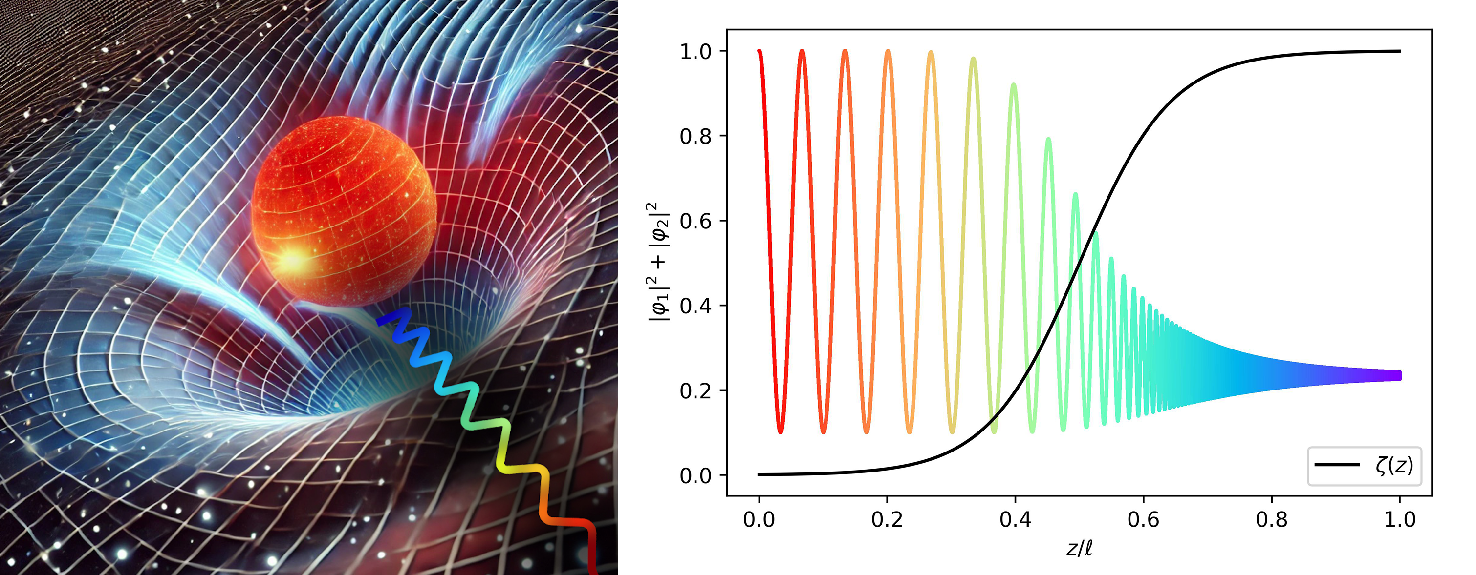
Given the above possibility of synthesizing PG metric in solids, how do the corresponding ”gravity-like” aspects manifest in spectroscopies? One of the salient predictions of Einstein’s general relativity was that the photons (despite being massless), when climb up a gravitational potential, loose their energy , thereby getting red-shifted [35] as in Fig. 1. Within Newtonian mechanics this would make sense only if the photon had mass. For a massless particle, the gravitational red-shift can be explained in terms of an underlying curved spacetime. This tiny shift [37] involving fractional frequency changes of the order was measured in 1959 by Pound and Rebka [36] using high-accuracy measurement enabled by Mössbauer effect.
The purpose of this paper is to theoretically demonstrate a similar effect in a solid-state setup for massless Dirac electrons without using general relativity’s computational tools. The remarkable aspect of the present solid-state gravitational red-shift is that the fractional change in this case can be on the scale of or larger. Such a red-shift like behavior of Dirac electrons in solids can be similarly considered to be one possible indicator of an underlying emergent spacetime geometry. A change of variable from the original Dirac spinor to a convenient spinor acts like a change of frame of reference from ”substrate frame” where the transport experiment is being conducted, to a locally non-tilted frame of reference.
Recent advance in the theoretical interpretation of zero-bias photocurrents in spin-orbit-coupled surface Dirac cones of topological insulators -— attributed to frame transformations [34], promises exciting prospects for inducing strong position-dependent tilts via magnetic domain walls. The smooth variation of tilt not only minimizes impedance mismatch, leading to nearly perfect transmission, but also unlocks the potential for tilted Dirac cone junctions to act as tunable devices—capable of red- or blue-shifting electron waves depending on whether the tilt profile follows an upswing or downswing along the junction. This introduces a novel concept for wavelength up- or down-conversion in conducting media, harnessing abstract gravitational concepts to enable useful applications – distinct from traditional semiconductor-based approaches.
The paper is organized as follows: In section II we discuss the boundary conditions and the transformation that simplifies the Dirac equation in variable tilt background. In section III we formulate the transport coefficients in the transformed spinor basis. Section IV we present numerical results and our WKB-like approximate analytic treatment. In section V we compute the transmission coefficient that is accessible in transport measurements. We end the paper in section VI by a summary and outlook.
II Alternative representation of the Hamiltonian
In this section, we derive an alternative representation of the Hamiltonian that can comfortably give the continuity equation necessary to describe the behavior of massless Dirac fermions in two-dimensional (2D) materials with position-dependent tilting. Let us start with the conventional expression of the Hamiltonian for massless Dirac fermions in a 2D system with a constant tilt the -direction [34]
| (1) |
where and denote the Fermi and tilt velocities, respectively, while and represent the well-known Pauli matrices, and is the identity matrix. For later convenience we have rotated the standard representation of the Dirac equation in the plan around the axis to obtain a representation in the plane. This form of the Hamiltonian has the advantage that it can be rewritten as
| (2) |
where
| (3) |
and is the tilting parameter that is driven by the coefficient of the unit matrix that has been now absorbed into the above matrix . This transformation is an essential step of the present work that facilitates derivation of analytical expressions, along with plausible numerical solutions of the ensuing wave equations. The above form can now be nicely generalized to a situation with spatially variable . As particles propagate through the medium, the Hamiltonian must be constructed to ensure the corresponding continuity equation is satisfied. With this crucial requirement in mind, and based on the Hamiltonian provided in Eq. (2), it is reasonable to introduce the desired Hamiltonian as
| (4) |
It is important to note that, since the tilting parameter is a function of , the matrix also depends on , and the derivative with respect to acts on this matrix as well. This equation is similar to the way position-dependent mass in semiconducting heterostructure are handled [38, 39, 40], although generalizations can be possible by allowing the arbitrary powers with for the two such that in the spirit of corresponding position-dependent mass problems [40]. Similar forms of the Hamiltonian as in Eq. (4) have been used in Refs. [41] and [42] for the Dirac equation with a -dependent Fermi velocity. In fact Eq. (4) at the expense of introducing a -dependent matrix , appears like a Dirac equation for a locally upright Dirac cone. In that respect it can be considered as a solid-state physicist way of introducing Einstein’s vielbeins (or frame fields) [43]. As we will see in Eq. (26), this transformation allows to write current densities that in the new (local) basis looks like corresponding expressions for upright Dirac cones. Therefore this important equation secretly has a frame field content.
Using our representation of the Hamiltonian in Eq. (4) the continuity equation is
| (5) |
where the probability density, , and the probability current density are
| (6) |
where is the two-component (spinor) wave function, and and are unit vectors in the - and -directions, respectively. In the general case, , , and are functions of both position and time. However, for the sake of brevity, this dependence is not explicitly shown in the equations above. The Hamiltonian in Eq. (4), the continuity equation in Eq. (5), and the expressions for and in Eq. (6) are all mutually consistent. Furthermore the Hamiltonian (4) is Hermitian in the sense that [44].
The specific case where is constant has been thoroughly studied in our previous work [45]. That study examined the behavior of massless Dirac particles as they cross the boundary between two materials with different tilt parameters, the occurrence of Klein tunneling, and the spin rotation angle of these particles after crossing the interface. In the present work, we extend this investigation to the case where varies as a function of .
III Transmission Probability and Klein Tunneling
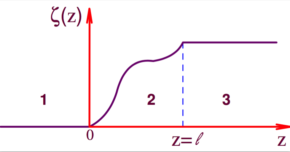
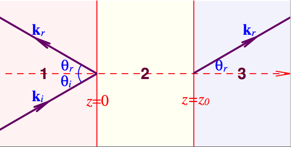
Using the Hamiltonian and the associated continuity equation for tilted Dirac cones with spatially varying tilt parameters, we can explore the transport in heterostructure composed schematically depicted in Fig. 2. In this figure, three regions labeled are separated by a region labeled within which the tilt varies in space. The corresponding tilts in general can be , , and . The middle layer has a thickness of , while the outer layers extend infinitely. In the setup we have studied, region is assumed to have no tilt, i.e. where the Dirac fermions represented by upright Dirac cones. In region , the tilt continuously varies starting from in its left end and continuously reached in its right end. The shape of variations can be any continuous function schematically displaced in Fig. 2.
The Schrödinger eigenvalue equation, which governs the behavior of massless Dirac fermions in the various regions of the setup depicted in Fig. 2, is expressed in its general form as
| (7) |
where represents the eigenfunction of corresponding to the energy eigenvalue . The -axis is considered to be normal to the interface of the media. In this configuration, due to the translation invariance in the direction, the is conserved, and will be of the following form
| (8) |
For this class of wave functions, the Schrödinger eigenvalue equation for the middle region simplifies to
| (9) |
Defining the new spinor by
| (10) |
Eq. (9) becomes
| (11) |
To develop some intuition to the structure of solutions, first consider the normal incidence of massless Dirac fermions from region onto the interface. In this case, the particles travel along the -axis, so . Furthermore a complete scattering state can be considered by setting the spinor part of the wave function and consequently to have only one non-zero component, i.e. their spinor part is proportional to either or . For example consider the first case where which corresponds to the boundary conditions
| (12) |
Eq. (11) reduces to
| (13) |
where represents the element in row and column of the matrix . The solution to this equation, under the boundary conditions of Eq. (12), is
| (14) |
where
Finally, using Eq. (10), is determined as
| (15) |
Eq. (15) shows that the -component of the probability current density, , remains constant, signifying the occurrence of Klein tunneling. In this scenario, which corresponds to normal incidence at the interface, there is a perfect transmission probability, allowing all particles to traverse the central slab and enter the third medium.
If instead the boundary conditions are
| (16) |
then in the above equations, should be replaced by and the corresponding eigen-spinor must be replaces by .
Next, let us consider a more general case. As illustrated in the right panel of Fig. 2, we assume that massless Dirac fermions travel through medium and strike the interface with the middle slab at an arbitrary angle. Our goal is to calculate the reflection and transmission probabilities for these states as they traverse the intermediate region.
Referring to the right panel of Fig. 2, the wave function of the system in the outer regions is
| (17) |
where
| (18) |
where subscripts , and , refer to incident, reflected and transmitted waves, respectively. The coefficients and represent the reflection and transmission amplitudes. The angles , , and , termed the angles of incidence, reflection, and transmission, respectively 222Note that for the upright Dirac cones, the direction of wave vectors are the same as group velocities, whereas in the tilted Dirac cone case they are not the same. We choose to parameterize the angular variables refering to the wave vectors [45]. as shown in Fig. LABEL:Fig02. Correspondingly, the wave vectors associated with the incident, reflected, and transmitted waves are denoted as , , and .
The components of these wave vectors in the -direction (normal to the interface) are , , and , while their components in the -direction are , , and . Due to translational invariance along direction, all the -components of the wave vectors are equal and therefore they are all specified with a single vlaue
| (19) |
It is crucial to note that the value of -components of wave vectors adjust themselves to satisfy the boundary conditions that ensure continuity equation. The value of depends on the tilting parameter in region 3. Moreover, the energy is also converted in all regions and in region 1 where there is no tilting, we have:
| (20) |
allowing us to easily determine and .
To compute , we note that in region 3, the Schrödinger eigenvalue equation from the Hamiltonian in Eq. (1) is
| (21) |
The eigenvalues of the operator on the left-hand side are . Since we are considering waves propagating to the right (), we choose the positive eigenvalue. Setting this eigenvalue equal to , we obtain
| (22) |
which is an implicit equation for that can be solved for . With the -components of the incident, reflected, and transmitted wave vectors, along with the known angles of incidence, reflection, and transmission, the wave functions , , and are uniquely determined.
To fully characterize the wave function of the system outside the central slab, it is crucial to determine the amplitudes and defined in Eq. (17). This requires a detailed analysis of the wave function behavior within the central region. By examining this wave function and applying the continuity conditions, the values of and can be precisely determined. To achieve this, we utilize Schrdöinger’s equation for a fixed energy , as given by Eq. (11) for the central slab region. In this region, the wave function is represented as a two-component spinor
| (23) |
In the middle slab (), Eq. (11) can be separated into two coupled first-order differential equations governing and :
| (24) |
where the coefficients , , and are defined as:
| (25) |
For arbitrary variable functions of satisfying the appropriate boundary conditions (as illustrated in Fig. 2), these coupled first-order differential equations can be numerically solved to desired accuracy. The boundary conditions are derived from the continuity of the -component of the probability current density at the interfaces. Using the expression for from Eq. (6), we can express the -component of the current density as:
| (26) |
As pointed out below Eq. (4), the last line looks like the current density for a locally upright Dirac cone. Therefore the new spinor defined by Eq. (10) can be interpreted as a spinor in a locally Minkowski spacetime. As such, the matrix defined in Eq. (4) encapsulates a transformation to a locally flat Minkowski spacetime.
To proceed with the question of boundary conditions, since , it follows that is continuous across all regions, including at the interfaces. In particular, at the interface between regions 2 and 3 (), this continuity implies:
| (27) |
where and are the Fermi velocities in regions 2 and 3, respectively. This boundary condition is essential to obtain unique numerical solutions and of the coupled differential equaitons (24). In this work we will assume that all regions have the same Fermi velocity .
By applying the continuity condition at the boundary , the following expression is derived:
| (28) |
This equation consists of two coupled algebraic equations the solution of which readily gives the amplitudes of reflection () and transmission (),
| (29) |
With these amplitudes, the reflection and transmission probabilities and can be readily computed:
| (30) |
Needless to say, they satisfy .
IV Results and Discussion
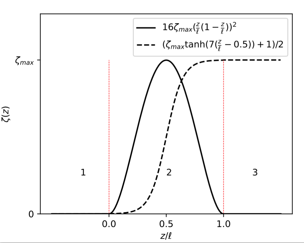
In this section, we perform a detailed analysis of the solution to the set of differential equations in Eqs. (24). We begin by examining a heterojunction composed of three regions where regions and have two uniform tilts as shown in Fig. 3. The middle layer has a position-dependent tilt. In our work we have considered two distinct tilting textures and for ”bump” and ”sigmoid” shaped functions given by
| (31) |
where is a parameter that we take at most to be , and represents the length of the middle layer, measured in units of . Note that due to linear energy-momentum scaling, fixing the energy , fixes this natural unit for the length. Therefore the length and energy are not independent variables. Studying the problem at higher (lower) or smaller (larger) means that a fixed value, e.g. in units of will correspond to longer (shorter) physical lengths for the variable-tilt region. For the sigmoid shaped tilting profile we choose,
| (32) |
which introduces an alternative tilting profile. Both functions are displayed in Fig. 3 where is shown by solid lines and by dashed line.
Next, we solve the set of Eqs. (24) by considering an incoming electron with a given wave vector . It is clear that , and therefore, will be determined according to Eq. (27). This provides the boundary conditions for the equations at and allows us to numerically find the solutions of these equations.
Due to the complex structure of the spinors and , the final solutions of the system are parameterized as
| (33) |
where , where and are usual spherical angles which for a spinor are given by
The angles and can be regarded as the polar and azimuthal angles of the spinors in locally flat Minkowski spacetime. In the following, we present numerical results for , , and obtained using the 4th-order Runge-Kutta method.
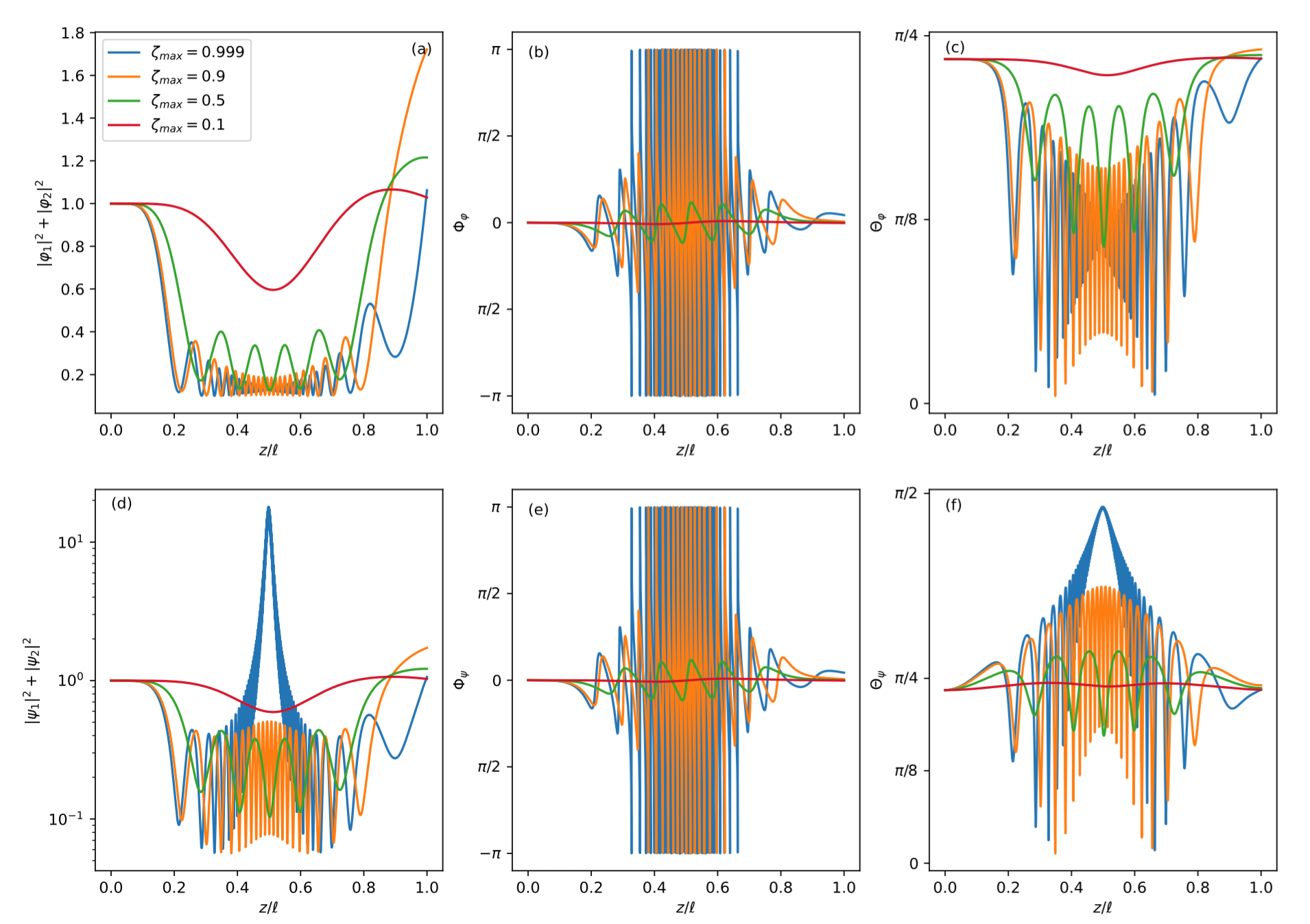
We choose the parameter of the incident wave and take the length of the middle layer to be (in units of ). The corresponding numerical solutions are presented in Fig. 4. The first row of panels, labeled (a), (b), and (c), displays , , and as functions of for four different values of the tilt heights: which specifies the height of the bump. As can be seen upon increasing the magnitude of the bump, more oscillations are induced to all of these quantities as a function of the dimensionless length . Another salient feature of all the figures of the top row that represent the spinor components and the spherical angles as a function of position is that for large enough where enough oscillations are formed, the wave length of the oscillations are smaller in the center of the bump whereas the wave lengths are larger (i.e. red-shifted) away from the bump. Note that the normalization of is such that the continuity equation holds. The physically observable transmission coefficients are calculated based on the ratios of the amplitudes at beginning and end of the middle region, and this normalization does not pose any issues.
As pointed out the spinor represents the wave function in a local frame. It is useful to transform it back to the original frame (that can be dubbed substrate frame to emphasize its solid state context) by the defining relation . The results are shown in second row as panels (d), (e), and (f) of Fig. 4. For clarity, we use the notations and for the spherical angles of , and and for those of .
Notably, in both frames the oscillation are faster in the regions where the local value of is larger which is reminiscent of ”gravitational” red-shift pattern. As can be seen this behavior manifests itself in both local frame () and substrate frame (). In particular, the oscillation patterns of the azimuthal angle and are quite similar. Note that the azimuthal angles are with respect to -axis that also denotes the direction of transport. Therefore the azimuthal angles both represent transverse precession in the local frame and and the substrate frames.
The behavior of polar angle that represents the orientation of the spinor with respect to the motion direction is however quite different which can be seen from the comparison of panels (c) and (f). Let us begin by noting the similarities in the wavelength of the oscillations: both panels clearly share the red-shift behavior. In the substrate frame, as can be seen in panel (f), by increasing the bump strength in the center of the middle region where can reach its value, the average value around which the oscillations is taking place is lifted upward. For (blue curve) that is very close to the ”horizon” value of this enhancement of the and its tendency to ”equator” value of is more manifest in panel (f). This means that in the substrate frame first of all the horizon is indicated as locking of the polar angle to equatorial value, and secondly the nodding amplitude is suppressed more and more. The suppression of the nodding amplitude is also seen in panel (c) that represents the polar angle in local frame. However, in this frame the saturation value of the polar angle is which is much smaller than the equatorial value.
A comparison can also be made between panels (a) and (d) that represent the total probability constructed from both components of the spinors in local and substrate frames, respectively. Again as can be seen both frames display clearly the red-shift pattern in their wave lengths. In the local frame as can be seen in panel (a), the average value around which the oscillations are taking place approaches a fixed value at the center where has its maximum value. The approach to horizon is remarkably reflected in the behavior of the probability in panel (d) as a strong peak (note the logarithmic scale in panel d). Comparing panel (d) against (a), can be seen that the approach to the critical value can be diagnosed in the substrate coordinate in which the solid-state measurements are done. Local frame that moves along with the electron wave is only a mathematically convenient frame for the computation.
Combining the information from and the probability if one has a local probe of pseudospin, the enhancement of the local can be inferred from both the noting amplitude as well as the strength of the signal that will be directly controlled by the square of wave function.
IV.1 Analytical result for the position-dependent oscillations
Can one understand the above numerical results analytically? It turns out that the answer is yes, and a very illuminating physical picture emerges. To address the physical origin of position-dependent or equivalently -dependent oscillations, we focus on a small enough interval of where the function can be approximated as constant. Within this interval, the Schrödinger equation (9) for , derived from Eq. (23), takes the form:
| (34) |
where is the identity matrix. Now in the spirit of WKB approximation, we seek solutions of the form where depends on and hence local value of . Substituting this ansatz into Eq. (34), we obtain two eigenvalues for denoted by and which are given by:
| (35) |
By transforming the Pauli matrix to local frame, namely we have and and . As a result, the eigenvalues and in Eq. (34) are identical to those of:
| (36) |
where the spinors in the two frames are related by .
Let the eigenfunctions of Eq. (36) be and , and those of Eq. (34) be and . The relationship between these eigenfunctions is given by
| (37) |
where the subscripts in the right hand side indicate the first and second spinor components. This relation shows that the eigenfunctions and in the local frame are not orthogonal and the amount of non-orthogonality is determined controlled by the amount of tilt parameter vanishing for .
If the initial state of the system is chosen as a linear combination of the eigenbasis, i.e., , the norm of varies with as:
| (38) |
where . This result demonstrates that oscillates periodically as a function of , and for a sufficiently large length, it may even return to its initial value.
This analysis even allows to extrapolate to neighboring point . The solution in an adjacent interval can be expressed as:
| (39) |
where . It is evident that even small changes in alter the norm of . Furthermore, it can be shown that the expectation value of is conserved, i.e., , since . This result is consistent with the earlier discussion on current density conservation. Algebraically it derives from the fact that sicne both and are diagonal matrices, the Pauli matrix in both substrate frame and local frame is the same. While the norm of oscillates with , it can also acquire a phase factor due to precession around the -axis.
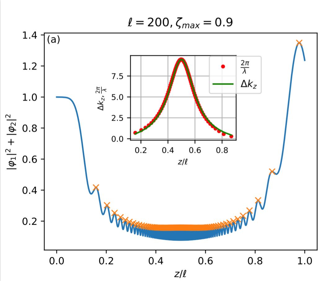
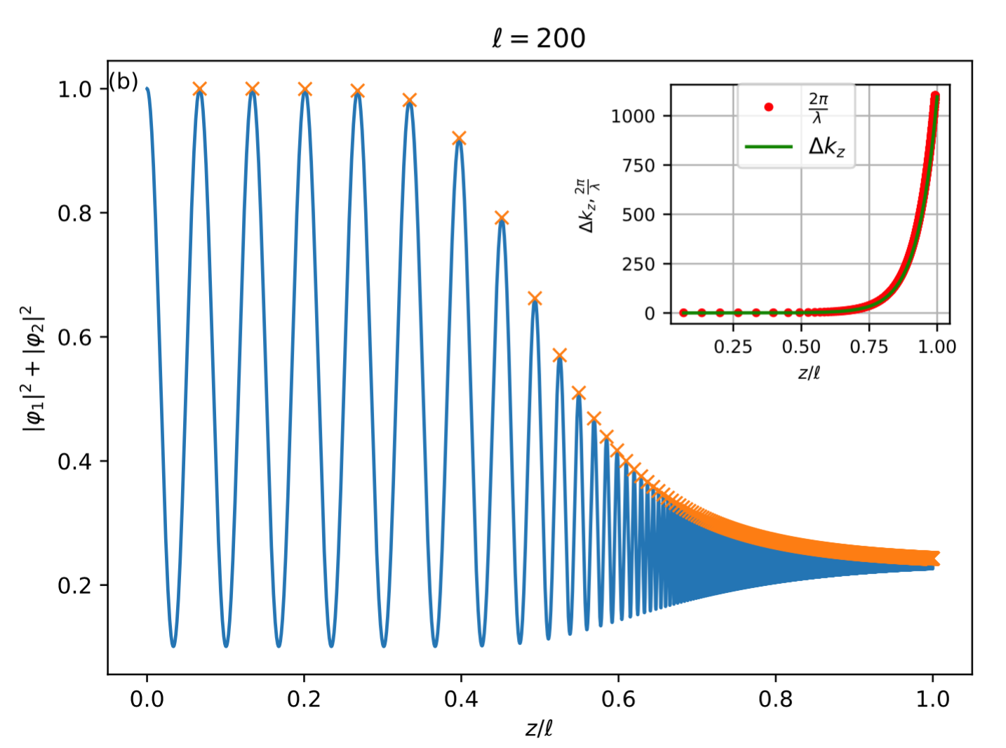
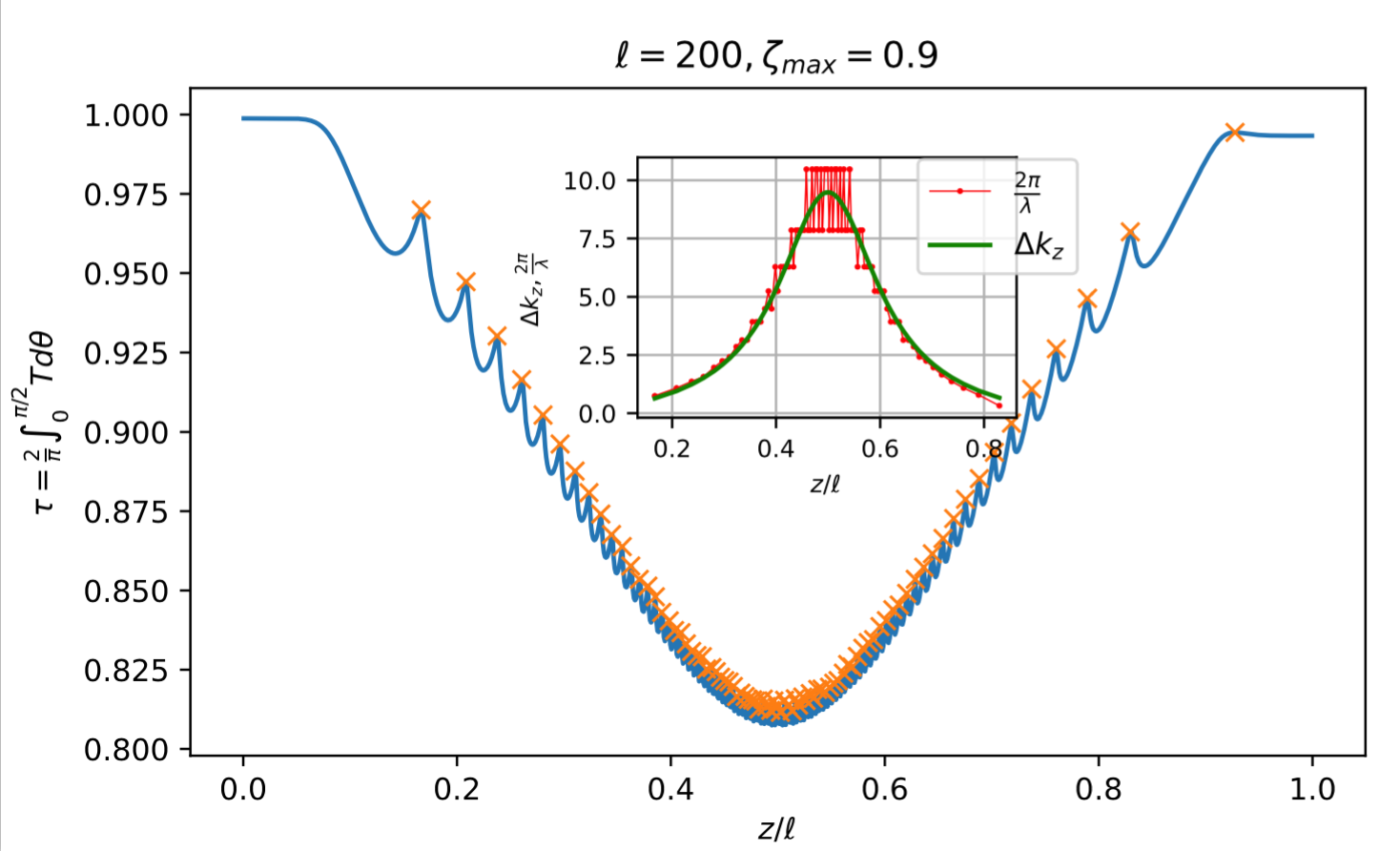
To corroborate the above analytical result with numerical computations, in Fig. 5 for a middle layer with we examine the variation in for the two tilting functions (top panel (a)) and (bottom panel (b)) defined in Eqns. (31) and (32) and for the incident wave with . The oscillation peaks in Fig. 5 are marked by orange crosses. By locating the positions of adjacent peaks we determined the wavelength from which the wave number is obtained as . In the insets the wave numbers for both and are compared with the following analytic expression :
| (40) |
As can be seen a very good agreement between this analytic wave numbers and numerical results for both tilting functions can be achieved. Panel (b) further indicates that the red-shift behavior is not limited to the bumped tilt texture. Such a red-shift behavior can be considered as a probe of the local value of . Our analysis confirms that similar wave numbers can be obtained for other quantities, such as and .
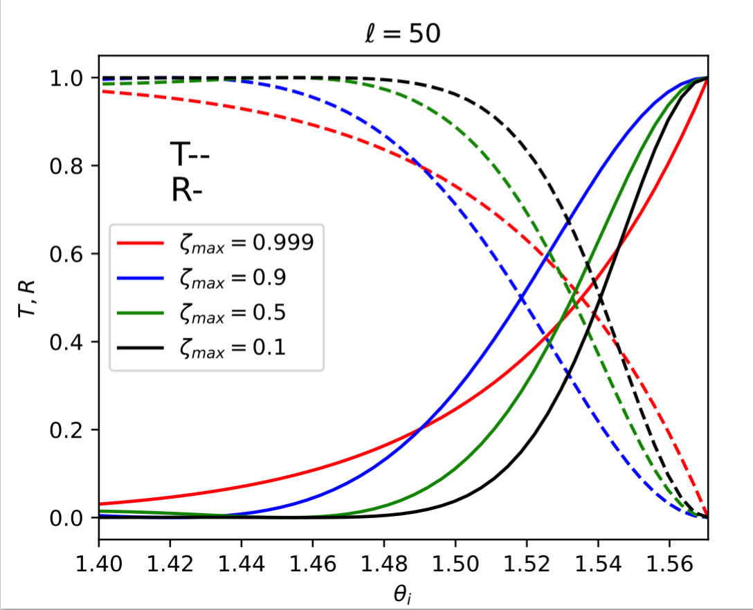
Before concluding this section, it is worth addressing why for the bump profile which is symmetric around , the solutions are not symmetric; specifically, why are the solutions at the boundaries and not identical, even though layers 1 and 3 are equivalent? The asymmetry arises from the reflected waves: while the solutions of the equations in the set (24) are periodic, there is always a reflected wave, and not all of the incident waves are transmitted. This partial reflection leads to an asymmetrical profile in the solution. Figure 6 illustrates the transmission () and reflection () coefficients, calculated using Eqs. (30), for a fixed and different values of , as functions of in an interval close to . Furthermore, as pointed out, the spinor corresponds to a local frame. This local frame at every point can be considered as a upright Dirac cone moving with velocity [34]. As such, one moving direction is preferred and hence the two directions along and opposite to moving velocity are not equivalent, although the profile of magnitude looks symmetric.
V Transport measurement of red-shift pattern
To suggest a tangible experimental trace of the above red-shift features, in Fig. 7 we have computed the integrated transmission that quantifies the fraction of the incident wave transmitted through the tilted region by
where is the angle-dependent transmission coefficient. For this analysis, we evaluate at various positions within the tilted region, representing the fraction of the length that the wave has traversed.
Fig. 7 shows as a function of for the tilting function . As expected the redshift behavior obtained for a fixed value of the incident wave parameter , persists after integrating over . Again the left-right asymmetry continues to hold in illustrating the complex interplay between wave reflection and transmission within the tilted region. These oscillations arise from the interference of waves as they propagate and reflect, and they persist even though the external layers are equivalent. The inset of Fig. 7 highlights the corresponding wavenumber, extracted from the oscillatory behavior of . Interestingly, the wavenumber matches perfectly with as previously discussed and shown in the inset of Fig. 5. But here we are dealing with -integrated version of numerical and analytical results. This agreement confirms the consistency of the observed oscillatory behavior across different physical quantities, further validating our analytical predictions regarding .
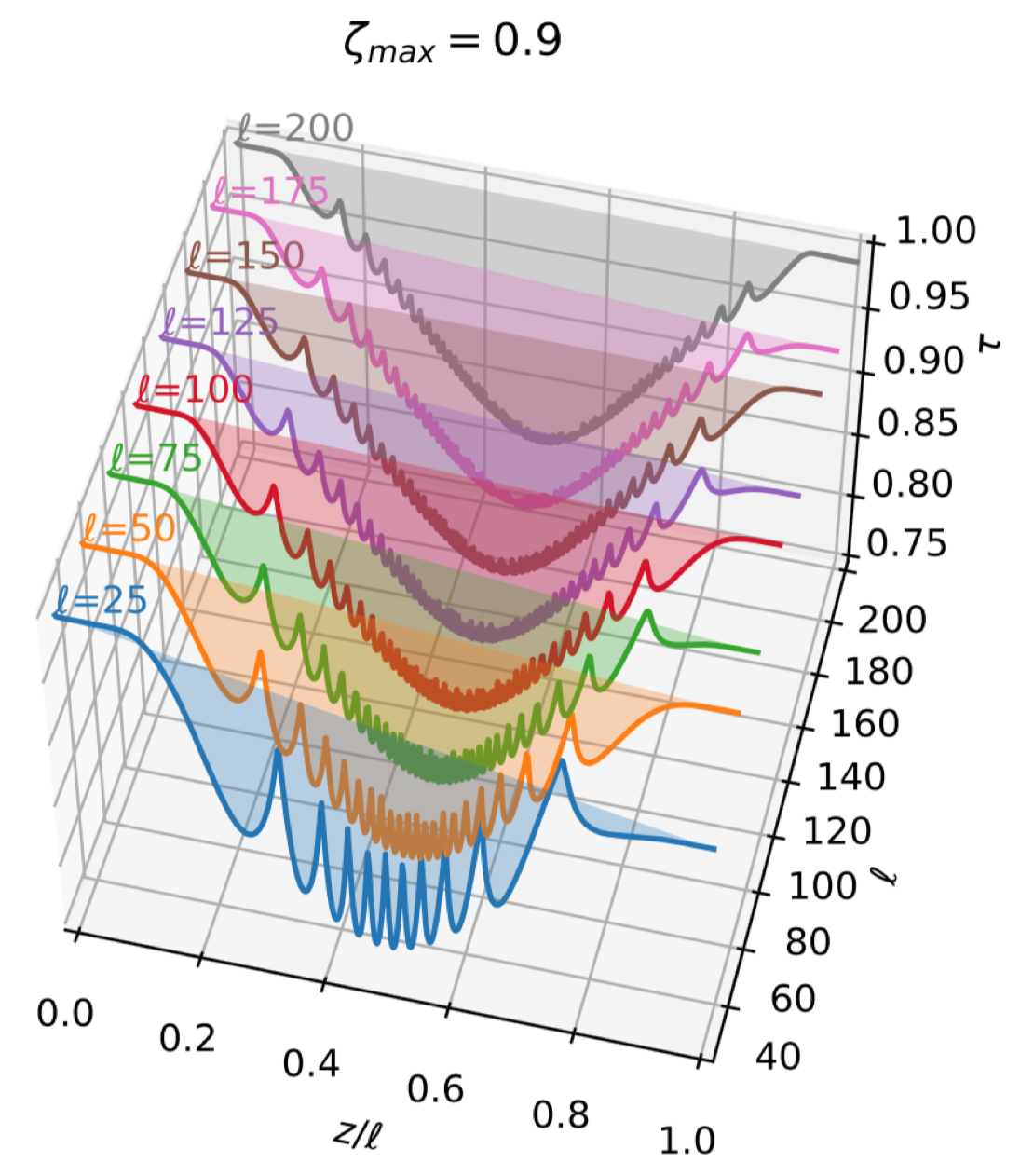
The above results are obtained for a fixed value of the energy . For the fixed that also fixes the unit of length , it means that the physical length of the middle layer hosting the variable tilt medium is . For example when eV and m/s, would correspond to nm. One could ask what happens when the physical junction length becomes thiner. This computation has been plotted in Fig. 8 where the integrated transmission has been plotted for smaller length scales down to nearly an order of magnitude smaller length scale of that at eV corresponds to nm. The following points can be observed in the figures:
-
1.
For all the above length scales, the redshift pattern is manifest, i.e. by moving away from the bump, the wave length of the oscillations increases.
- 2.
-
3.
The number of peaks scales linearly with as given in table 1 and fits remarkably well to the formula . This means that although the wave length undergoes a red-shift pattern away from the bump center, the total number of oscillations for the bump-shaped tilting profile manages to scale with the length of the junction.
-
4.
As can be clearly seen, by spreading the bump over a longer junction amplitude of the oscillations steadily decreases for larger . One can extrapolate from Fig. 8 that for very large junction length , the transmission curve becomes a smooth curve.
| 10 | 20 | 30 | 40 | 50 | 60 | 70 | 79 | |
| 25 | 50 | 75 | 100 | 125 | 150 | 175 | 200 |
The property (2) above rests on the fact that gradual change in that gives rise to gradual change in velocity, produces small impedance mismatch [46], thereby diminishing the reflection and enhancing the transmission. This property can be employed as engineering concept in designing media to convert electron wave number while the nearly perfectly transmit. The wave length of the incident and transmitted waves are red-/blue-shifted depending on the step direction of the sigmoid profile. This concept is similar to the graded-index optical fiber [47, 48].
For larger , the bump in Fig. 3 spreads over a longer distance, and therefore the spatial variations of , namely on average becomes smaller. In such a situation, the property (4) above means that the amplitude of the oscillations are controlled by the derivative . Such derivatives appear in the Christoffel connections that govern the motion of waves in the ray-optics limit.
In experimental setup measuring the conductance one usually synthesizes one sample with a fixed and there is not much room to change the . How can the above results be useful? As pointed out, the linear scaling of energy and momentum implies that for a physical junction with a given length, the dimensionless number that counts the number of fitting into the physical junction, can be decreased by increasing . Therefore moving to lower corresponds to moving from gray plot to blue plot in Fig. 8. This can be done in the lab by sweeping the voltage in a scanning tunneling spectroscopy: Scanning along the junction can probe various positions, whereas scanning the energy from low to high voltages amounts to scanning from blue to gray curves of Fig. 8. Measuring the tunneling current at a fixe energy as a function of will give a typical redshift pattern of the form displayed in Fig. 7. Increasing the voltage and scanning again the junction width would lead to (i) increase in the number of peaks, and (ii) decrease in the amplitude of oscillations as in Fig. 8. For example doubling the voltage and scanning the junction width to is expected to double the number of peaks within the junction as suggested by table 1.
VI Summary and outlook
Tilt of Dirac cones is a proxy for an emergent spacetime metric where tilting parameter directly appears in the off-diagonal components of the spacetime metric that mix space and time coordinates. When an underlying metric is present, it must show up in various quantities. In this work we have computed the transmission of electron waves through a region where tilting has spatial profiles of bump and sigmoid shape in Fig. 3. We find features in the amplitude of the wave function, spherical angles of the pseudospin, and the transmission coefficients that resemble the ”gravitational redshift”. It means that the wave length of oscillatory behavior is smaller in regions with larger tilt and get (red) shifted to larger wave lengths in regions with smaller .
The ability to red- or blue-shift electron waves, in addition to demonstrating a general-relativistic effect in the lab, can find potential application: Since due to very low impedance mismatch that arises from gradual change of tilting, the reflection is diminished and the medium nearly perfectly transmits the waves a sigmoid tilting profile can be used to perfectly transmit electron waves and deliver them with red-/blue-shifted wave lengths.
Recent experimental evidence for the tilting induced by magnetic influence in the spin-orbit coupled Dirac cones at the surface of topological insulators [33, 34] is a promising platform to imprint spatially variable textures of tilting by a corresponding texture of the magnetization. The present proof of principle study indicates that aspects of the underlying spacetime geometry can be detected by standard solid-state spectroscopic tools. In the spin-orbit coupled Dirac cones, interesting oscillatory behavior of pseudo-spin orientation and the corresponding red-shift effects is expected to find novel applications in spintronics devices.
VII Acknowledgements
S.A.J. acknowledges the support of Hendrik J. Bluhm.
References
- Muechler et al. [2016] L. Muechler, A. Alexandradinata, T. Neupert, and R. Car, Topological nonsymmorphic metals from band inversion, Physical Review X 6, 10.1103/physrevx.6.041069 (2016).
- Isobe [2017] H. Isobe, Tilted dirac cones in two dimensions, in Theoretical Study on Correlation Effects in Topological Matter (Springer Singapore, 2017) p. 63–81.
- Kobayashi et al. [2007] A. Kobayashi, S. Katayama, Y. Suzumura, and H. Fukuyama, Massless fermions in organic conductor, Journal of the Physical Society of Japan 76, 034711 (2007).
- Varykhalov et al. [2017] A. Varykhalov, D. Marchenko, J. Sánchez-Barriga, E. Golias, O. Rader, and G. Bihlmayer, Tilted dirac cone on w(110) protected by mirror symmetry, Physical Review B 95, 10.1103/physrevb.95.245421 (2017).
- Lopez-Bezanilla and Littlewood [2016] A. Lopez-Bezanilla and P. B. Littlewood, Electronic properties of borophene, Physical Review B 93, 10.1103/physrevb.93.241405 (2016).
- Zhang et al. [2023] S.-H. Zhang, D.-F. Shao, Z.-A. Wang, J. Yang, W. Yang, and E. Y. Tsymbal, Tunneling valley hall effect driven by tilted dirac fermions, Physical Review Letters 131, 10.1103/physrevlett.131.246301 (2023).
- [7] Anisotropic longitudinal optical conductivities of tilted dirac bands in MoS2, .
- Park et al. [2022] S. H. Park, M. Sammon, E. Mele, and T. Low, Plasmonic gain in current biased tilted dirac nodes, Nature Communications 13, 10.1038/s41467-022-35139-y (2022).
- Jalali-Mola and Jafari [2018a] Z. Jalali-Mola and S. A. Jafari, Tilt-induced kink in the plasmon dispersion of two-dimensional dirac electrons, Physical Review B 98, 10.1103/physrevb.98.195415 (2018a).
- Jalali-Mola and Jafari [2018b] Z. Jalali-Mola and S. A. Jafari, Kinked plasmon dispersion in borophene-borophene and borophene-graphene double layers, Physical Review B 98, 10.1103/physrevb.98.235430 (2018b).
- Torbatian et al. [2021] Z. Torbatian, D. Novko, and R. Asgari, Hyperbolic plasmon modes in tilted dirac cone phases of borophene, Physical Review B 104, 10.1103/physrevb.104.075432 (2021).
- Mojarro et al. [2022] M. A. Mojarro, R. Carrillo-Bastos, and J. A. Maytorena, Hyperbolic plasmons in massive tilted two-dimensional dirac materials, Physical Review B 105, 10.1103/physrevb.105.l201408 (2022).
- Sengupta et al. [2018] P. Sengupta, Y. Tan, E. Bellotti, and J. Shi, Anomalous heat flow in 8-pmmn borophene with tilted dirac cones, Journal of Physics: Condensed Matter 30, 435701 (2018).
- KAWARABAYASHI et al. [2012] T. KAWARABAYASHI, Y. HATSUGAI, T. MORIMOTO, and H. AOKI, Generalization of chiral symmetry for tilted dirac cones, International Journal of Modern Physics: Conference Series 11, 145–150 (2012).
- Ohki et al. [2020] D. Ohki, M. Hirata, T. Tani, K. Kanoda, and A. Kobayashi, Chiral excitonic instability of two-dimensional tilted dirac cones, Physical Review Research 2, 10.1103/physrevresearch.2.033479 (2020).
- Gomes and Ramos [2021] Y. M. P. Gomes and R. O. Ramos, Tilted dirac cone effects and chiral symmetry breaking in a planar four-fermion model, Physical Review B 104, 10.1103/physrevb.104.245111 (2021).
- Zhao and Wang [2019] P.-L. Zhao and A.-M. Wang, Interplay between tilt, disorder, and coulomb interaction in type-i dirac fermions, Physical Review B 100, 10.1103/physrevb.100.125138 (2019).
- Mojarro et al. [2023] M. A. Mojarro, R. Carrillo-Bastos, and J. A. Maytorena, Thermal difference reflectivity of tilted two-dimensional dirac materials, Physical Review B 108, 10.1103/physrevb.108.l161401 (2023).
- Paul et al. [2019] G. C. Paul, S. F. Islam, and A. Saha, Fingerprints of tilted dirac cones on the rkky exchange interaction in 8- pmmn borophene, Physical Review B 99, 10.1103/physrevb.99.155418 (2019).
- Sinha [2019] D. Sinha, Spin transport and spin pump in graphene-like materials: effects of tilted dirac cone, The European Physical Journal B 92, 10.1140/epjb/e2019-90332-7 (2019).
- Suzumura et al. [2014] Y. Suzumura, I. Proskurin, and M. Ogata, Effect of tilting on the in-plane conductivity of dirac electrons in organic conductor, Journal of the Physical Society of Japan 83, 023701 (2014).
- Volovik and Zhang [2017] G. E. Volovik and K. Zhang, Lifshitz transitions, type-ii dirac and weyl fermions, event horizon and all that, Journal of Low Temperature Physics 189, 276–299 (2017).
- Volovik [2021] G. E. Volovik, Type-ii weyl semimetal versus gravastar, JETP Letters 114, 236–242 (2021).
- Liang and Ojanen [2019] L. Liang and T. Ojanen, Curved spacetime theory of inhomogeneous weyl materials, Physical Review Research 1, 10.1103/physrevresearch.1.032006 (2019).
- Zubkov [2018] M. Zubkov, Analogies between the black hole interior and the type ii weyl semimetals, Universe 4, 135 (2018).
- Volovik [2016] G. E. Volovik, Black hole and hawking radiation by type-ii weyl fermions, JETP Letters 104, 645–648 (2016).
- Kedem et al. [2020] Y. Kedem, E. J. Bergholtz, and F. Wilczek, Black and white holes at material junctions, Physical Review Research 2, 10.1103/physrevresearch.2.043285 (2020).
- Könye et al. [2022] V. Könye, C. Morice, D. Chernyavsky, A. G. Moghaddam, J. van den Brink, and J. van Wezel, Horizon physics of quasi-one-dimensional tilted weyl cones on a lattice, Physical Review Research 4, 10.1103/physrevresearch.4.033237 (2022).
- Farajollahpour and Jafari [2020] T. Farajollahpour and S. A. Jafari, Synthetic non-abelian gauge fields and gravitomagnetic effects in tilted dirac cone systems, Physical Review Research 2, 10.1103/physrevresearch.2.023410 (2020).
- Hashimoto and Matsuo [2020] K. Hashimoto and Y. Matsuo, Escape from black hole analogs in materials: Type-ii weyl semimetals and generic edge states, Physical Review B 102, 10.1103/physrevb.102.195128 (2020).
- Yekta et al. [2023] Y. Yekta, H. Hadipour, and S. A. Jafari, Tunning the tilt of the dirac cone by atomic manipulations in 8pmmn borophene, Communications Physics 6, 10.1038/s42005-023-01161-9 (2023).
- Ghorashi et al. [2020] S. A. A. Ghorashi, J. F. Karcher, S. M. Davis, and M. S. Foster, Criticality across the energy spectrum from random artificial gravitational lensing in two-dimensional dirac superconductors, Physical Review B 101, 10.1103/physrevb.101.214521 (2020).
- Ogawa et al. [2016] N. Ogawa, R. Yoshimi, K. Yasuda, A. Tsukazaki, M. Kawasaki, and Y. Tokura, Zero-bias photocurrent in ferromagnetic topological insulator, Nature Communications 7, 10.1038/ncomms12246 (2016).
- Jafari [2024] S. A. Jafari, Moving frame theory of zero-bias photocurrent on the surface of topological insulators, Physical Review Research 6, 10.1103/physrevresearch.6.033006 (2024).
- Einstein [1916] A. Einstein, Die grundlage der allgemeinen relativitätstheorie, Annalen der Physik 354, 769–822 (1916).
- Pound and Rebka [1959] R. V. Pound and G. A. Rebka, Gravitational red-shift in nuclear resonance, Physical Review Letters 3, 439–441 (1959).
- Ryder [2009] L. Ryder, Introduction to General Relativity (Cambridge University Press, 2009).
- Koç and Tütüncüler [2003] R. Koç and H. Tütüncüler, Exact solution of position dependent mass schrödinger equation by supersymmetric quantum mechanics, Annalen der Physik 515, 684–691 (2003).
- Mazharimousavi and Halilsoy [2013] S. H. Mazharimousavi and M. Halilsoy, One dimensional newton’s equation with variable mass (2013), arXiv:1308.2981 .
- Rosas-Ortiz [2020] O. Rosas-Ortiz, Position-dependent mass systems: Classical and quantum pictures, in Geometric Methods in Physics XXXVIII (Springer International Publishing, 2020) p. 351–361.
- Raoux et al. [2010] A. Raoux, M. Polini, R. Asgari, A. R. Hamilton, R. Fazio, and A. H. MacDonald, Velocity-modulation control of electron-wave propagation in graphene, Phys. Rev. B 81, 073407 (2010).
- Joy et al. [2020] S. Joy, S. Khalid, and B. Skinner, Transparent mirror effect in twist-angle-disordered bilayer graphene, Phys. Rev. Res. 2, 043416 (2020).
- Yepez [2011] J. Yepez, Einstein’s vierbein field theory of curved space (2011), arXiv:1106.2037 .
- Witten [2016] E. Witten, Three lectures on topological phases of matter, La Rivista del Nuovo Cimento 39, 313–370 (2016).
- Al-Marzoog et al. [2024] R. Al-Marzoog, A. Rezaei, Z. Noorinejad, M. Amini, E. Ghanbari-Adivi, and S. A. Jafari, Tilted dirac cones in two-dimensional materials: Impact on electron transmission and pseudospin dynamics, Phys. Rev. B 110, 165427 (2024).
- Howard [1992] G. Howard, The Physics of Waves (Benjamin Cummings, 1992).
- Gong et al. [2010] Y. Gong, T. Zhao, Y.-J. Rao, Y. Wu, and Y. Guo, A ray-transfer-matrix model for hybrid fiber fabry-perot sensor based on graded-index multimode fiber, Optics Express 18, 15844 (2010).
- Gong et al. [2014] Y. Gong, W. Huang, Q.-F. Liu, Y. Wu, Y. Rao, G.-D. Peng, J. Lang, and K. Zhang, Graded-index optical fiber tweezers with long manipulation length, Optics Express 22, 25267 (2014).