Static spherically symmetric solutions of the $f(R)$ gravity

Abstract

Static spherically symmetric (SSS) solutions of $f(R)$ gravity are studied in the Einstein frame. The solutions involve SSS configuration mass $M$ and scalaron mass $\mu$ (in geometrized units). For typical astrophysical masses, the dimensionless parameter $M\mu$ has very large value. We found analytic solutions on a finite interval for $M\mu\to\infty$ in case of a family of scalaron potentials. The asymptotically flat solutions on $(0,\infty)$ have been studied numerically for $M\mu$ up to $10^{20}$ in case of the quadratic $f(R)$ model.

Keywords: spherical symmetry, modified gravity, scalar fields

I Introduction

In the $f(R)$ gravity, the gravitational Einstein-Hilbert Lagrangian density is replaced by a more general function of the scalar curvature $R$ (see [1, 2, 3] for a review) . This leads to fourth-order equations with respect to the space-time metric $g_{\mu\nu}$ (Jordan frame). However, in a number of the $f(R)$ versions, it is possible to reduce the problem to usual Einstein equations with respect to new metric $\hat{g}_{\mu\nu}$ (Einstein frame) by means of conformal transformation [1, 2, 3]

$$\hat{g}_{\mu\nu}=e^{2\xi}g_{\mu\nu}\,,$$ (1)

where some scalar field $\xi$ dubbed scalaron satisfies an additional nonlinear wave equation that involves a scalaron mass $\mu$.

Natural questions arise concerning the possible role of the $f(R)$ gravity in compact astrophysical objects. Most publications on this subject deal with the black-hole configurations [5, 6, 7, 8, 9]. The static spherically symmetric (SSS) objects without a horizon have been investigated in [10, 4]. Such objects turn out to be either linearly stable or unstable depending on the choice of configuration parameters [4].

In different $f(R)$ theories, the scalaron masses vary from $\sim 10^{13}~\text{Gev}$ to $\sim 4~\text{meV}$ (see, e.g., [11, 12]). This yields very large dimensionless $M\mu$ (in geometrized units), where $M$ is the configuration mass. The latter, comparatively small, value of $\mu$ corresponds to length scale $l_{\mu}\sim 5\cdot 10^{-3}~\text{cm}$ yielding for the Solar mass $\mu M=M/l_{\mu}\simeq 3\cdot 10^{9}$ and another 8-9 orders of magnitude more for typical masses of the central objects in active galactic nuclei. This leads to exponentially large numbers and creates some difficulties for application of standard numerical algorithms to investigation of SSS configurations. Note that the numerical results obtained in [10, 4] in a case of the quadratic $f(R)$ model deal only with modest $M\mu$.

In this paper, we consider approximate SSS solutions for sufficiently large $M\mu$. For numerical estimates we use the scalaron potential of the quadratic $f(R)$ gravity [11], see also [12, 10].

This paper is organized as follows. In Section II, we review the relations of $f(R)$ gravity in the Einstein frame for SSS configurations. The basic equations in a suitable form for consideration of large $M\mu$ are presented in Section III. Then we justify the approximate solutions for a special class of the scalaron potentials IV. In Section V we perform numerical calculations to illustrate the solutions. In Section VI, we discuss our results.

II Basic equations in the Einstein frame

The well known example when the transition to the Einstein frame is possible by means of transformation (1) is due to the quadratic $f(R)$ [13, 11, 12]; the corresponding scalaron self-interaction potential $W(\xi)$ is [13, 11, 12];

$$W(\xi)=\mu^{2}w(\xi)\,,\quad w(\xi)=\frac{3}{4}\left(1-e^{-2\xi}\right)^{2}\,.$$ (2)

For the SSS space-time we use the Schwarzschild (curvature) coordinates

$$d\hat{s}^{2}\equiv\hat{g}_{\mu\nu}dx^{\mu}dx^{\nu}=e^{\alpha}dt^{2}-e^{\beta}dr^{2}-r^{2}dO^{2},$$ (3)

where $r>0$, $\alpha\equiv\alpha(r)$, $\beta\equiv\beta(r)$ and $dO^{2}=d\theta^{2}+\sin^{2}\theta d\varphi^{2}$ stands for the metric element on the unit sphere.

In absence of non-gravitational fields, the nontrivial equations for static metric (3) in the Einstein frame are (see, e.g., [4])

$$\frac{d}{dr}(\alpha+\beta) =6r\left(\frac{d\xi}{dr}\right)^{2}\,,$$ (4)

$$\frac{d}{dr}(\alpha-\beta) =-\frac{2}{r}+\frac{2e^{\beta}}{r}\left[1-r^{2}W(\xi)\right]\,.$$ (5)

where $\xi\equiv\xi(r)$. Equations (4), (5) for $\alpha$ and $\beta$ must be supplemented by an equation for scalaron $\xi$:

$$\frac{d}{dr}\left[r^{2}e^{\frac{\alpha-\beta}{2}}\frac{d\xi}{dr}\right]=\frac{r^{2}}{6}e^{\frac{\alpha+\beta}{2}}W^{\prime}(\xi)\,.$$ (6)

In the asymptotically flat static space-time, it is assumed that for $r\to\infty$ we have $\xi(r)\to 0$ and Eq. (6) can be approximated by the equation for the linear massive scalar field on the Schwarzschild background

$$\exp[\alpha(r)]=1-r_{g}/r,\quad\exp[\beta(r)]=(1-r_{g}/r)^{-1}\,,$$ (7)

where $r_{g}=2{M}$, where ${M}>0$ is the configuration mass. Formulas (7) are valid for $r\to\infty$, since $\xi\to 0$ tends to zero fairly quickly. However, this is not enough to determine the unique solution of the system (4),(5),(6) and additional information about $\xi(r)$ is needed. For large $r$, small $\xi(r)$ must decay exponentially with the asymptotic behavior [14, 15, 16]

$$\xi(r)=Q\left(\frac{r_{g}}{r}\right)^{1+M\mu}e^{-\mu r}\,.$$ (8)

The constant $Q$, which characterizes the strength of the scalar field at infinity, will be called the “scalar charge”. For given $M$ and $Q$, the asymptotic formulas (7),(8) determine the solution in a unique way [4].

In what follows we will restrict ourselves to positive $\xi$, where potential (2) has a plateau-like form; this form is preferable for physical reasons in view of cosmological data (see, e.g. [17]).

III Reduction of equations

From rigorous analytical considerations in case of a monotonous function $w(\xi)$, $\xi>0$ [4] (cf. also a case of a minimally coupled scalar field [18]), it follows that in any non-trivial case there must be some ”scalarization region”, where one can hope to see a smoking gun of the modified gravity. In case of the non-monotonous potentials (e.g., the hill-top potentials) numerical simulations show similar behavior at least for sufficiently large $M\mu$. We will focus on the astrophysically interesting case, when the size of this region is large enough, say $\sim(100\div 1000)r_{g}$. On the other hand, there must be an interval of small exponentially decaying $\xi(r)$ for $r\geq r_{0}$; the metric in this region quickly takes on the Schwarzschild values (7) as $r$ grows. This will be labeled as interval A. We assume that $r_{0}$ marks a boundary between these two regions and $\xi_{0}\equiv\xi(r_{0})$ is sufficiently small so as to use formulas (7), (45), (45) for $r\geq r_{0}$. For given $\xi(r_{0})$, the value of $r_{0}$ can be related with the scalar charge according to (45).

It may be difficult to perform direct numerical integration of the basic equations in the form (4),(5),(6) for $M\mu\gg 10^{12}$ with a standard software because of exponentially large numbers involved. In order to consider the problem for large $M\mu$, we introduce new independent variable $p$ by means of the relations

$$r\mu=X_{0}+\frac{p}{X_{0}}\equiv X_{0}U(p)\,,\,\,U(p)=1+\frac{p}{X^{2}_{0}}\,,$$ (9)

where $X_{0}=\mu r_{0}\gg 1$ and the interval $r\in(0,r_{0}]$ corresponds to negative $p\in(-X_{0}^{2},0]$. We will move from $p=0$ to negative values.

Denote

$$\chi=\frac{\alpha+\beta}{2}\,,\quad Y=U\exp\left(\frac{\alpha-\beta}{2}\right)$$ (10)

Equation (4) yields

$$\frac{d\chi}{dp}=3U\left(\frac{d\xi}{dp}\right)^{2}\,,$$ (11)

Equation (5) multiplied by $\exp[(\alpha-\beta)/2]$ can be transformed to

$$\frac{dY}{dp}=e^{\chi}\left[\frac{1}{X^{2}_{0}}-U^{2}w(\xi)\right]\,.$$ (12)

In terms of (9) and (10), from equation (6) we get

$$\frac{d}{dp}\left[UY\frac{d\xi}{dp}\right]=\frac{U^{2}}{6X_{0}^{2}}e^{\chi}w^{\prime}(\xi)\,.$$ (13)

By denoting

$$Z=-X_{0}UY\frac{d\xi}{dp}\,,$$ (14)

we obtain from (13) two first-order equations

$$\frac{d\xi}{dp}=-\frac{Z}{X_{0}UY}\,,$$ (15)

$$\frac{dZ}{dp}=-\frac{U^{2}}{6X_{0}}e^{\chi}w^{\prime}(\xi)\,.$$ (16)

Substitution of (15) into (11) yields

$$\frac{d\chi}{dp}=\frac{3Z^{2}}{UY^{2}}\,.$$ (17)

Now we have a closed system of four equations (12),(15),(16),(17) in a normal form, which is ready for the backwards numerical integration, starting from $p=0$. Correspondingly, we set initial data at $p=0$, which corresponds to $r=r_{0}>r_{g}$:

$$\xi(0)=\xi_{0}\,,\,\,\quad Y(0)\equiv Y_{0}=\exp\left[\frac{\alpha_{0}-\beta_{0}}{2}\right]\,,$$

$$\chi(0)=\chi_{0}\,,\quad Z_{0}=-X_{0}Y_{0}\left(\frac{d\xi}{dp}\right)_{0}$$ (18)

From (44) we get

$$Z_{0}=-X_{0}Y_{0}\left(\frac{d\xi}{dp}\right)_{0}=\xi_{0}\exp{(\alpha_{0}/2)}\,,$$ (19)

where $\alpha_{0}=\alpha(0)$.

IV Approximate solution

The aim of this Section is to present a family of approximate analytic solutions of (12),(15),(16),(17) in some interval $r\in(0,r_{0}]$, $r_{0}>>r_{g}$, which can be useful to check numerical methods.

We consider a class of potentials (2), where

$$w(\xi)=3\xi^{2}(1+O(\xi))\,,\,\,w^{\prime}(\xi)=6\xi(1+O(\xi))$$ (20)

for $|\xi|<<1$; also

$$|w(\xi)|\leq w_{0}<\infty\,,\,\,|w^{\prime}(\xi)|\leq w_{1}<\infty\,,$$ (21)

and

$$\gamma(\xi)=1-\frac{w(\xi)}{3\xi^{2}}>0\,,\quad\xi>0,$$ (22)

where $w_{0},\,w_{1}$ and $\gamma(\xi)=O(\xi)$ do not depend on $\mu$. These properties are fulfilled in case of the quadratic $f(R)$ gravity [13, 11], however, the scope of application of the results following from these conditions is much wider; with some caveats it covers, e.g., the case of the hill-top and table-top potentials listed in [17].

The initial conditions for the scalaron field and metric well be imposed at $r_{0}$ corresponding to (7), (45). We fix $r_{0}$ and $\xi_{0}:0<\xi_{0}\ll 1$ and consider limit $M\mu\to\infty$. In this Section we do not discuss the condition of the asymptotic flatness and corresponding solutions for $r\geq r_{0}$, which may impose additional restrictions on $\xi_{0}$.

Consider the transition region B, where

$$\xi(p)\approx\xi_{0},\quad Z(p)\approx Z_{0},\quad U(p)\approx 1.$$ (23)

We will see that to satisfy these relations it is sufficient to restrict $p$ as follows: $0>p>p_{1}\simeq-\sqrt{X_{0}}$.

For sufficiently large $M\mu$, the $X_{0}^{-2}$ term in the right-hand side of (12) can be neglected and equations (12),(17) yield

$$\frac{d\chi}{dp}=\frac{3Z^{2}}{Y^{2}}\,,\quad\frac{dY}{dp}=-e^{\chi}w(\xi)\,.$$ (24)

Combining these equations, we have

$$\frac{1}{Y^{2}}\frac{dY}{dp}=-\frac{w(\xi_{0})}{3Z^{2}_{0}}e^{\chi}\frac{d\chi}{dp}\,,$$

whence

$$\frac{1}{Y(p)}=\frac{1}{Y_{0}}+\frac{w(\xi_{0})}{3Z_{0}^{2}}\left[e^{\chi(p)}-e^{\chi_{0}}\right]\,.$$ (25)

In view of (19) and (22)

$$e^{\chi_{0}}\frac{Y_{0}}{Z_{0}^{2}}=\frac{1}{\xi_{0}^{2}}\,,\quad 1-\frac{Y_{0}w(\xi_{0})}{3Z_{0}^{2}}e^{\chi_{0}}=\gamma(\xi_{0})>0$$

Then

$$\frac{Y_{0}}{Y}\approx\frac{1}{Y_{*}}+e^{\chi-\chi_{0}}\,,\quad Y_{*}=\frac{1}{\gamma(\xi_{0})}\,.$$ (26)

Now let us assume that for $r=r_{0}$ the metric takes on the Schwarzschild values, so $\chi_{0}=0$, $|\beta_{0}|\ll 1$. Using (26) and $Z\approx Z_{0}$ from (19), equation (17) can be integrated to obtain

$$\ln\left(\frac{\gamma(\xi_{0})+e^{\chi}}{\gamma(\xi_{0})+1}\right)-\chi- \frac{\gamma(\xi_{0})(1-e^{\chi})}{[\gamma(\xi_{0})+e^{\chi}][\gamma(\xi_{0})+1]}$$

$$=-\frac{3\gamma^{2}(\xi_{0})}{Y_{0}}\xi_{0}^{2}X_{0}^{2}\ln\left(\frac{r}{r_{0}}\right)$$ (27)

where we take account of $\chi(0)=0$. From this we have inequality for $-\sqrt{X_{0}}\leq p\leq 0$

$$\chi(p)\lesssim-3\frac{\gamma^{2}(\xi_{0})}{Y_{0}}\,\xi_{0}^{2}\,|p|\,.$$ (28)

Using (28) and (21), for $-\sqrt{X_{0}}\leq p\leq 0$ we get from (16), because of the factor $X_{0}^{-1}$ in the right-hand side of this equation,

$$|Z(z)-Z_{0}|\leq\frac{C_{1}(\xi_{0})}{X_{0}}\,,\quad|p|\leq\sqrt{X_{0}}\,,$$ (29)

and using (26), from (15)

$$|\xi(p)-\xi_{0}|\approx\frac{Z_{0}}{X_{0}}\left(\gamma(\xi_{0})+e^{\chi}\right)\leq\frac{C_{2}(\xi_{0})}{\sqrt{X_{0}}}\,,$$ (30)

where $-\sqrt{X_{0}}\leq p\leq 0$ and constants $C_{1}(\xi_{0}),C_{2}(\xi_{0})$ do not depend on $X_{0}$. These are rough estimates, but they are sufficient for further consideration in case of $X_{0}\to\infty$ and fixed $\xi_{0}$ to justify approximations (23) in the region (B).

Owing to (28), for $p_{1}=-\sqrt{X_{0}}$, fixed $\xi_{0}$ and large enough $M\mu$

$$\exp[\chi(p_{1})]<\exp{(-3\gamma^{2}(\xi_{0})Y_{0}\xi_{0}^{2}\sqrt{X_{0}})}\ll\gamma(\xi_{0})\,;$$ (31)

this means that $Y(p)$ practically reaches maximal value $Y_{*}$ in the interval B.

Now we can consider interval C, where $p<p_{1}$ and we can deal with the exact equations (12) and (16). In consequence of (17) function ${\chi(p)}$ is monotonous, therefore $\exp{\chi(p)}<\exp{\chi(p_{1})}$ is bounded by very small constant

$$e^{\chi(p)}<\exp{\left(-3\frac{\gamma^{2}(\xi_{0})}{Y_{0}}\,\xi_{0}^{2}\,\sqrt{X_{0}}\right)}$$ (32)

This value enters into right-hand sides of (12) and (16) as an exponentially small factor for $X_{0}\to\infty$. Though we have a very large interval of $p\in(-X_{0}^{2},p_{1})$, this factor suppresses these right-hand sides and leads to practically constant values in interval C

$$Y(p)=Y_{S}\equiv\lim\limits_{r\to 0}Y(r)\,,\quad Z(p)=Z_{S}\equiv\lim\limits_{r\to 0}Z(r)\,,$$ (33)

and

$$Z_{S}\approx Z_{0},\quad Y_{S}\approx Y_{0}Y_{*}\,,$$ (34)

for $M\mu\gg 1$. On account of definitions (10) of $Y$ and (14) of $Z$, this means

$$r\exp\left(\frac{\alpha-\beta}{2}\right)\approx const,\quad r\frac{d\xi}{dr}\approx const$$ (35)

with very good accuracy for large $M\mu$. Formula (27) can be extended for $p<p_{1}$, i.e. to all interval C. Owing to the above estimates we get from (15) in this region (including $r\to 0$)

$$\xi(r)=-\frac{\xi_{0}}{\sqrt{Y_{0}}}\gamma(\xi_{0})X_{0}\ln\left(\frac{r}{r_{0}}\right)+\xi_{0}\,,$$ (36)

and from (17)

$$\chi(r)=3\frac{\xi_{0}^{2}}{Y_{0}}\gamma^{2}(\xi_{0})X_{0}^{2}\ln\left(\frac{r}{r_{0}}\right)\,.$$ (37)

The metric coefficients in the Einstein frame are obtained according to (1), (10):

$$e^{\alpha}=\frac{Y_{0}}{\gamma(\xi_{0})}\left(\frac{r}{r_{0}}\right)^{H-1}\,,\quad e^{\beta}=\frac{\gamma(\xi_{0})}{Y_{0}}\left(\frac{r}{r_{0}}\right)^{H+1}\,,$$ (38)

where $H\equiv 3\xi_{0}^{2}\gamma^{2}(\xi_{0})X_{0}^{2}/Y_{0}\gg 1$ for $M\mu\gg 1$ and fixed $\xi_{0}$.

Numerical tests have been carried out in case of the scalaron potential of the quadratic model (2), it satisfies conditions (20), (21), (22) for $\xi>0$. We compared numerical calculations with previous analytic relations for $\xi_{0}\sim 10^{-3}\div 10^{-5}$, $r_{0}\sim(10\div 1000)r_{g}$, $M\mu\sim 10^{5}\div 10^{25}$. Numerical simulations confirm that approximate formulas (33),(34) in region C hold with a good accuracy for $M\mu\gtrsim 10^{11}$. Examples of dependence of limiting parameter $Y_{S}$ upon $M\mu$ are shown in Fig. 1 for different sizes of the scalarization region corresponding to different values of the scalar charge. Asymptotics at large $M\mu$ are in good agreement with formula (26).

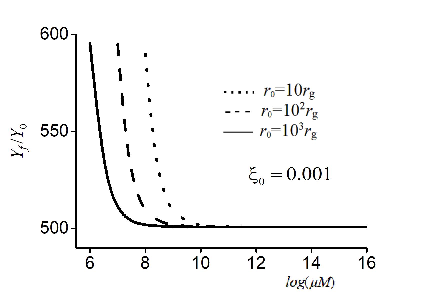
Figure 1: The case of potential (2): dependence of limiting value $Y_{S}/Y_{0}$ upon $M\mu$ for three sizes $r_{0}$ of the scalarization region determined by condition $\xi(r_{0})=0.001$.

V Numerical simulations

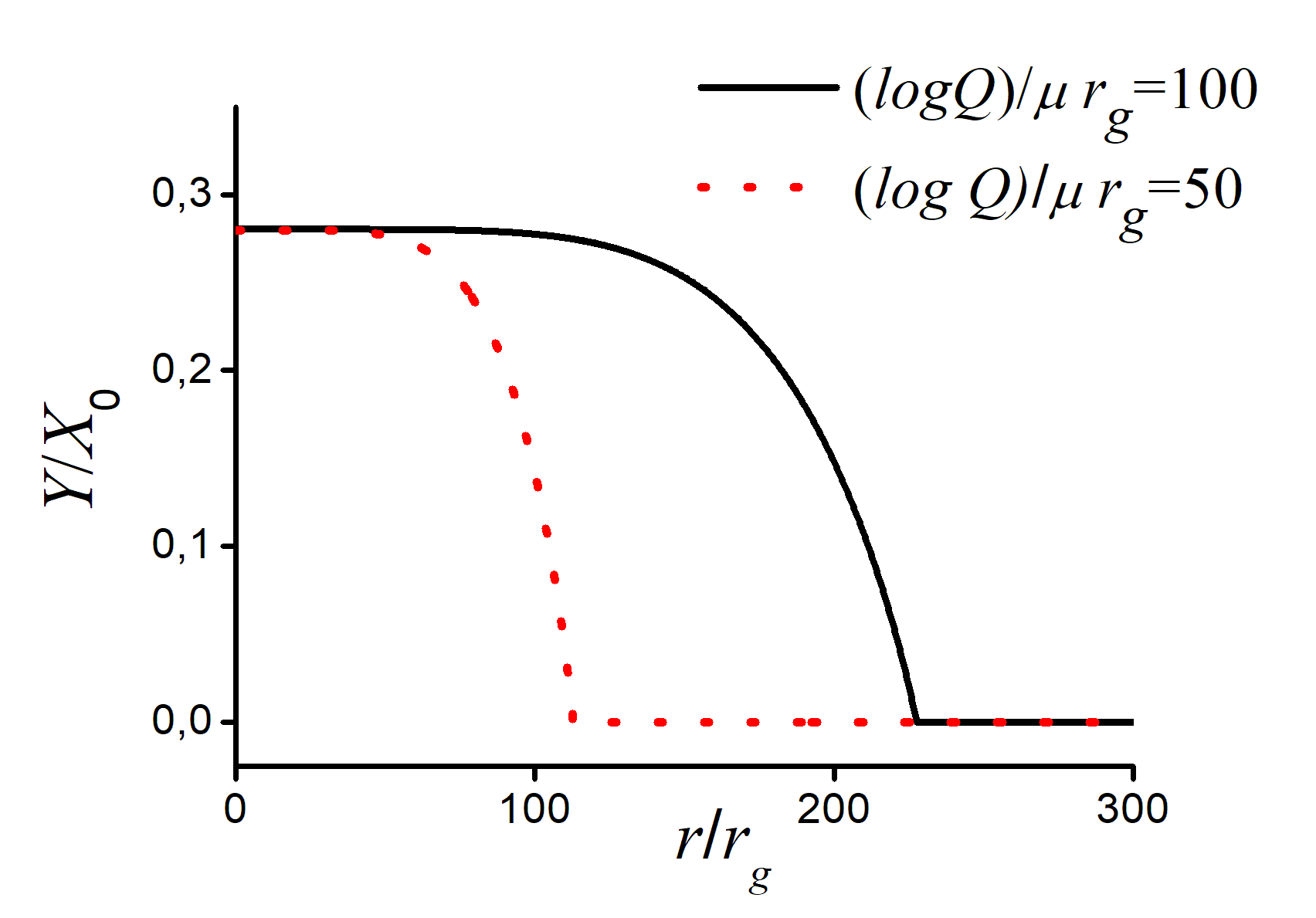
Figure 2: The case of potential (2): $Y(r)/X_{0}$ against $r/r_{g}$ for $\log Q=10^{22}$ and $\log Q=2\cdot 10^{22}$. In this calculation we used $\mu=10^{20}$, however the curves look almost the same for for $\log(\mu)=10\div 20$. Corresponding sizes of the scalarization region are $113r_{g}$ and $228r_{g}$; outside this area there is an increase in $Y(r)$ that is not visible here.

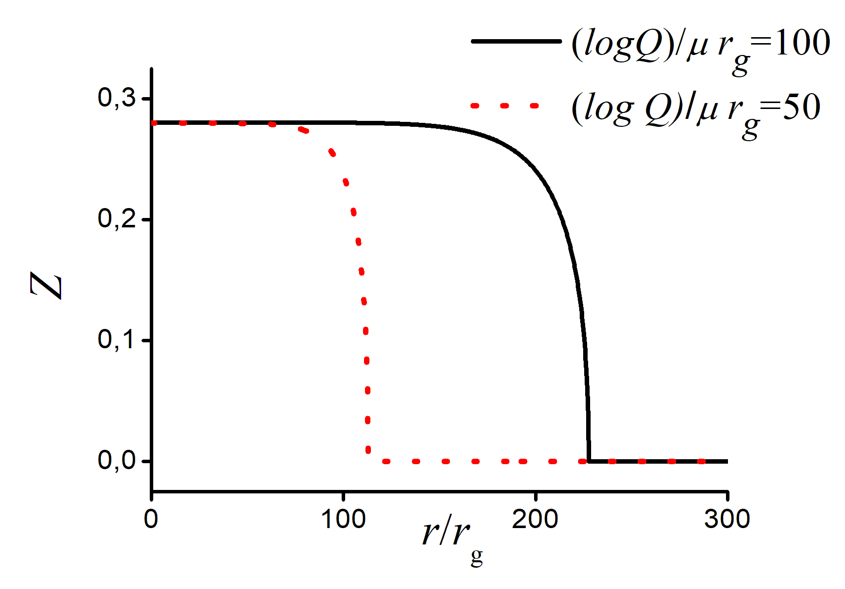
Figure 3: The case of potential (2): $Z(r)$ against $r/r_{g}$ for the same parameters as in Fig. 2. Outside the scalarization region region $Z(r)>0$ tends to zero exponentially. The curves look the same for $\log(\mu)=10\div 20$.

Figure 4: The case of potential (2): $\alpha(r)$ against $r/r_{g}$. A: $\log Q=2\cdot 10^{22}$; B: $\log Q=10^{22}$. The curves look the same for $\log(\mu M)=10\div 20$. Outside the scalarization region $\alpha(r)\approx-r_{g}/r$.

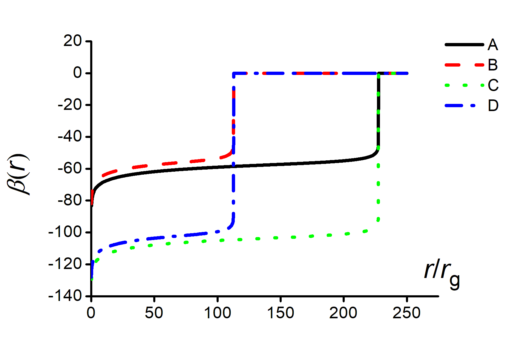
Figure 5: The case of potential (2): $\beta(r)$ against $r/r_{g}$. A: $\mu M=10^{20}$, $\log Q=2\cdot 10^{22}$; B: $\mu M=10^{20}$, $\log Q=10^{22}$; C: $\mu M=10^{10}$, $\log Q=2\cdot 10^{22}$; D: $\mu M=10^{10}$, $\log Q=10^{22}$. Outside the scalarization region $\beta(r)\approx r_{g}/r$.

The results of the previous Section with fixed $\xi_{0}$ and $M\mu\to\infty$ give some idea of the structure of SSS configurations. However, the statement of the problem must be modified in case of asymptotically flat SSS systems because $\xi_{0},M\mu$ and $r_{0}$ are correlated. The value $\xi_{0}$ must satisfy inequality (47) in order that the weak-field approximation (45) and/or (8) can be used up to $r\to r_{0}+0$. Therefore, in further numerical simulations we set the initial conditions as follows:

$$\xi(r_{0})=\frac{\tilde{\xi}_{0}}{\sqrt{X_{0}}},$$ (39)

where $\tilde{\xi}_{0}\ll 1$. We remind that we consider the positive branch of $\xi$. Under condition (39) the considerations of Section IV are no longer valid and the size of the intermediate transition region B for $X_{0}\to\infty$ is not small. In this case asymptotic values $Y_{S}$, $Z_{S}$ (33) also exist (see Figs. 2) and 3), but relation between these values and configuration parameters $M,Q$ must be derived numerically. The existence of limits (33) is ensured by the rapid decrease of $e^{\chi}\approx e^{\beta}$ as r decreases (see Figs. 4, 5). The behavior of $\xi(r)$ is shown in Fig. 6.

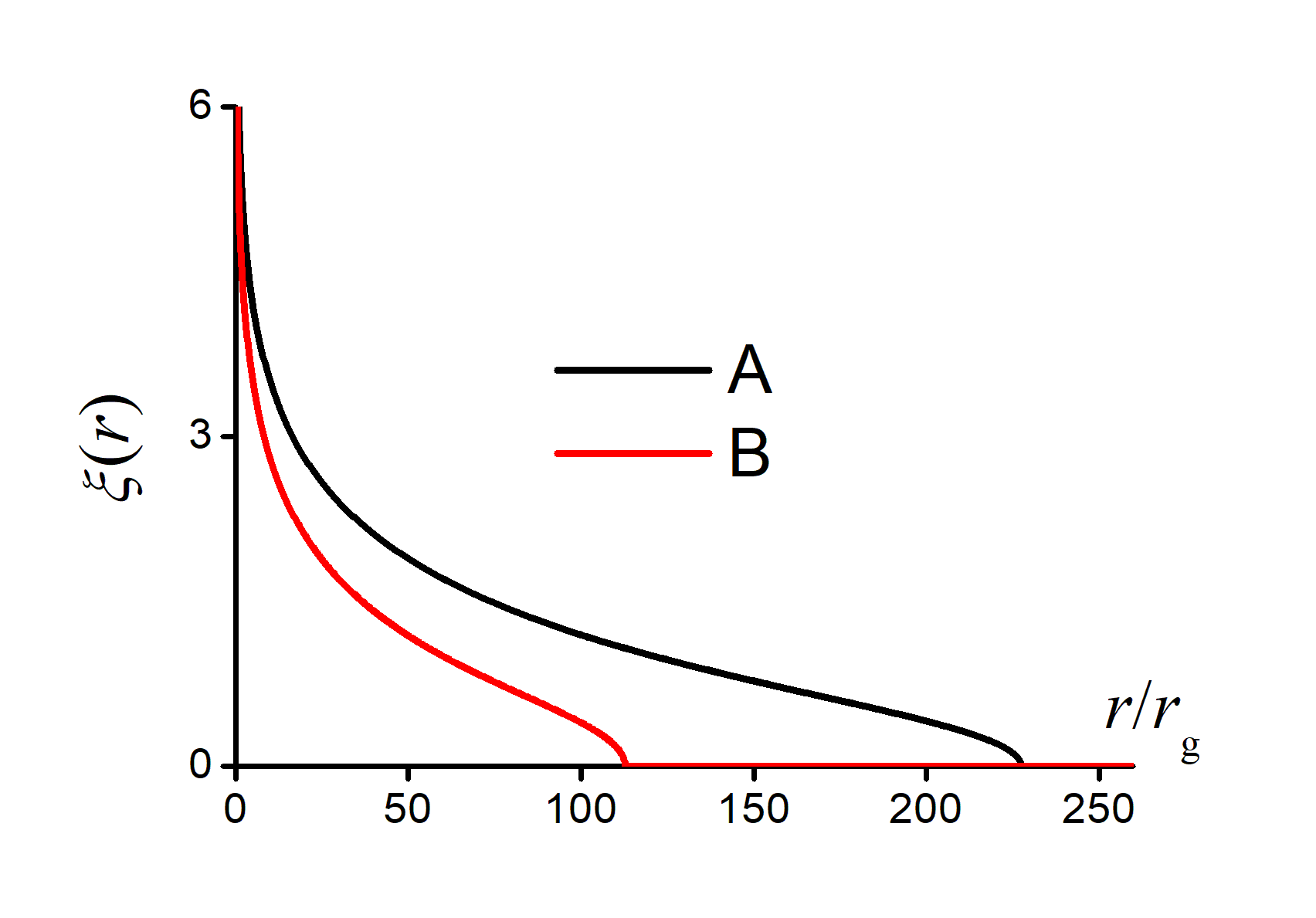
Figure 6: The case of potential (2): $\xi(r)$ against $r/r_{g}$. A: $\mu M=10^{20}$, $\log Q=2\cdot 10^{22}$; B: $\mu M=10^{20}$, $\log Q=10^{22}$. The curves look the same for $\log(\mu M)=10\div 20$. Outside the scalarization region $\xi(r)$ is given by (8).

VI Discussion

We studied SSS configurations in the Einstein frame of the $f(R)$ gravity and found a representation of the basic equations that allowed us to derive approximate solutions and to perform numerical calculations for rather high values of $M\mu$.

In case of potentials satisfying conditions (20),(21), (22) that are typical for a number of known $f(R)$ gravity models, for fixed data at some $r_{0}\gg r_{g}$, $0<\xi_{0}\ll 1$ and large enough $M\mu$, the SSS solutions exhibit similar behavior on $(0,r_{0}]$ that can be described analytically. The key formulas are (26), (34). Comparison with numerical simulations is shown in Fig. 1.

In case of asymptotically flat systems, there are three main regions of the radial variable with different types of behavior of the solutions.

In the region A ($r\geq r_{0}\gg r_{g}$), we have small scalaron field that decays exponentially according to (45). The metric takes on the Schwarzschild values.

Region B. This is an intermediate region of $r$ with a rapid change of the metric near $r_{0}$ with subsequent (with decreasing $r$) smooth transition to asymptotic values (33) in the region C closer to the origin. Regions B and C are significantly different from the Schwarzschild case. In C we have practically constant values of $rd\xi/dr$ and $r\exp((\alpha-\beta)/2)$.

Our results have been obtained in the Einstein frame. The metric coefficients in the Jordan frame can be obtained by the formula (1).

Acknowledgements. I am grateful to Yu. Shtanov and O. Stashko for useful discussions. This work was partially supported by the National Research Foundation of Ukraine under project No. 2023.03/0149.

Appendix A Approximate solutions in the region A

For $|\xi|\ll 1$ the scalaron potential and its derivative are approximated by (20) and equation (6) can be written as

$$\frac{d}{dr}\left[r^{2}e^{\frac{\alpha-\beta}{2}}\frac{d\xi}{dr}\right]=\mu^{2}r^{2}e^{\frac{\alpha+\beta}{2}}\xi\,.$$ (40)

For large $M\mu\gg 1$ we can apply the WKB method. Substitution of $\xi(r)=\exp[\mu u]$ into (40) we have

$$\left(\frac{du}{dr}\right)^{2}+\frac{1}{\mu}\frac{d^{2}u}{dr^{2}}+\frac{1}{\mu}\left[\frac{d}{dr}\left(2\ln r+\frac{\alpha-\beta}{2}\right)\right]=e^{\beta}$$ (41)

Putting $u(r)=u_{0}(r)+\mu^{-1}u_{1}(r)+...$ in zeroth order in $\mu^{-1}$ leads to

$$\frac{du_{0}}{dr}=-e^{\beta/2}$$ (42)

where we taken into account the asymptotic behavior at the infinity. In the next order

$$u_{1}(r)=-\ln r-\alpha/4+Const\,.$$ (43)

up to terms of the order of $(M\mu)^{-1}$.

Using (42) yields

$$\frac{d\xi}{dr}=-{\mu\xi}e^{\beta/2}\left[1+O\left(\frac{1}{M\mu}\right)\right]\,.$$ (44)

If $M\mu\gg 1$ and $\xi\ll 1$, in case of the Schwarzschild metric (7) we get

$$\xi(r)=\frac{Q(4/e)^{M\mu}\exp\left(-\mu r\sqrt{1-\frac{r_{g}}{r}}\right)}{(1-\frac{r_{g}}{r})^{1/4}\left(1+\sqrt{1-\frac{r_{g}}{r}}\right)^{\mu r_{g}}}\left(\frac{r_{g}}{r}\right)^{1+M\mu},$$ (45)

which is true up to terms of order $(M\mu)^{-1}$. This formula leads to (8) for $r\gg r_{g}$, However, for $M\mu\gg 1$, (45) is effective for $r>r_{g}$ comparable to $r_{g}$, provided that $\xi$ is small enough not affect the metric via (4),(5).

Now we must investigate how $\xi(r)$ affects $\alpha(r)$ and $\beta(r)$ under tha conditions of the asymptotic flatness. We assume here $r\gg r_{g}$.

Using (7) as zeroth approximation, the first order correction to $\chi(x)$ is obtained from (4) taking into account either (8) or (45)

$$\chi(r)=-3\int\limits_{r}^{\infty}dr^{\prime}r^{\prime}\left(\frac{d\xi}{dr}\right)^{2}\,\approx-\frac{3}{2}\mu r\xi^{2}(r)\,.$$ (46)

Therefore, in order that $|\chi_{0}|\ll 1$, one must have

$$X_{0}\xi_{0}^{2}\ll 1\,.$$ (47)

Also, under condition (47) one can infer from (5) that $|e^{-\alpha_{0}}(1-r_{g}/r_{0})-1|\ll 1$, $|e^{\beta_{0}}(1-r_{g}/r_{0})-1|\ll 1$. In this case one can be sure that for $r\geq r_{0}$ we can use formulas (7) and (45). In this case (47) shows that one cannot choose $M\mu$ sufficiently large without changing $\xi_{0}$.

References

- Sotiriou and Faraoni [2010] T. P. Sotiriou and V. Faraoni, theories of gravity, Reviews of Modern Physics 82, 451 (2010), arXiv:0805.1726 [gr-qc] .
- De Felice and Tsujikawa [2010] A. De Felice and S. Tsujikawa, theories, Living Reviews in Relativity 13, 3 (2010), arXiv:1002.4928 [gr-qc] .
- Nojiri et al. [2017] S. Nojiri, S. D. Odintsov, and V. K. Oikonomou, Modified gravity theories on a nutshell: Inflation, bounce and late-time evolution, Phys. Rept. 692, 1 (2017), arXiv:1705.11098 [gr-qc] .
- Zhdanov et al. [2024] V. I. Zhdanov, O. S. Stashko, and Y. V. Shtanov, Spherically symmetric configurations in the quadratic f (R ) gravity, Phys. Rev. D 110, 024056 (2024), arXiv:2403.16741 [gr-qc] .
- de La Cruz-Dombriz et al. [2009] A. de La Cruz-Dombriz, A. Dobado, and A. L. Maroto, Black holes in theories, Phys. Rev. D 80, 124011 (2009), arXiv:0907.3872 [gr-qc] .
- Bhattacharya [2016] S. Bhattacharya, Rotating Killing horizons in generic gravity theories, General Relativity and Gravitation 48, 128 (2016), arXiv:1602.04306 [gr-qc] .
- Cañate [2017] P. Cañate, A no-hair theorem for black holes in gravity, Classical and Quantum Gravity 35, 025018 (2017).
- Nashed and Nojiri [2020] G. G. L. Nashed and S. Nojiri, Nontrivial black hole solutions in gravitational theory, Phys. Rev. D 102, 124022 (2020), arXiv:2012.05711 [gr-qc] .
- Nashed and Nojiri [2021] G. G. L. Nashed and S. Nojiri, Specific neutral and charged black holes in gravitational theory, Phys. Rev. D 104, 124054 (2021), arXiv:2103.02382 [gr-qc] .
- Hernandéz-Lorenzo and Steinwachs [2020] E. Hernandéz-Lorenzo and C. F. Steinwachs, Naked singularities in quadratic gravity, Phys. Rev. D 101, 124046 (2020), arXiv:2003.12109 [gr-qc] .
- Starobinsky [1980] A. A. Starobinsky, A new type of isotropic cosmological models without singularity, Phys. Lett. B 91, 99 (1980).
- Shtanov [2021] Y. Shtanov, Light scalaron as dark matter, Physics Letters B 820, 136469 (2021), arXiv:2105.02662 [hep-ph] .
- Cembranos [2009] J. A. R. Cembranos, Dark matter from gravity, Phys. Rev. Lett. 102, 141301 (2009), arXiv:0809.1653 [hep-ph] .
- Asanov [1968] R. A. Asanov, Static scalar and electric fields in Einstein’s theory of relativity, Soviet Journal of Experimental and Theoretical Physics 26, 424 (1968).
- Asanov [1974] R. A. Asanov, Point source of massive scalar field in gravitational theory, Theoretical and Mathematical Physics 20, 667 (1974).
- Rowan and Stephenson [1976] D. J. Rowan and G. Stephenson, The massive scalar meson field in a Schwarzschild background space, Journal of Physics A Mathematical General 9, 1261 (1976).
- Shtanov et al. [2023] Y. Shtanov, V. Sahni, and S. S. Mishra, Tabletop potentials for inflation from gravity, J. Cosmol. Astroparticle Phys. 03, 023 (2023), arXiv:2210.01828 [gr-qc] .
- Zhdanov and Stashko [2020] V. I. Zhdanov and O. S. Stashko, Static spherically symmetric configurations with nonlinear scalar fields: Global and asymptotic properties, Phys. Rev. D 101, 064064 (2020), arXiv:1912.00470 [gr-qc] .