Monte Carlo model of distilled remote entanglement between superconducting qubits across optical channels

Abstract

A promising quantum computing architecture comprises modules of superconducting quantum processors linked by optical channels via quantum transducers. To map transducer device performance to system-level channel performance, our model uses Monte Carlo simulations that incorporate 2-to-1 and 3-to-1 entanglement distillation protocols. We show that the Extreme Photon Loss distillation protocol is particularly high performing and that, even without distillation, present-day transducers are at the threshold of enabling Bell pair distribution with fidelities of 50%. If the next generation of transducers can improve by 3 orders of magnitude in both added noise and efficiency, and increase repetition rates by 50$\times$, then they would allow for remote two-qubit gates achieving 99.7% fidelities at 100 kHz rates. These results set targets for transducers to be ready for deployment into scaled superconducting quantum computers.

I Introduction

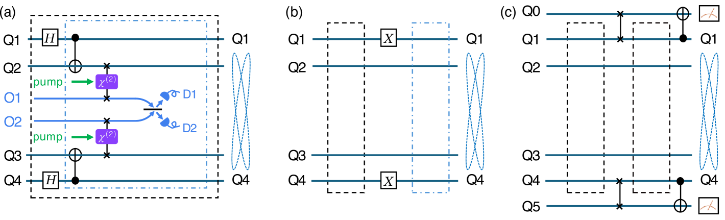
Figure 1: Circuit diagrams for different remote entanglement procedures. (a) The 1-click protocol using four superconducting qubits (Q1-Q4). Q1 and Q4 are the data qubits that are to be remotely entangled. Q2 and Q3 are the interface qubits that are swapped to optical photon channels O1 and O2 via the quantum transducer (denoted $\chi^{(2)}$). After upconversion, the optical photons are sent to detectors D1 and D2 through a 50:50 beamsplitter. (b) The 2-click protocol comprises two 1-click protocols with with an intervening $\pi$-pulse. The dashed boxes are instances of the 1-click protocol from (a). (c) Remote entanglement with the EPL distillation protocol. A Bell pair is heralded and swapped to memory qubits Q0 and Q5. After creation of second Bell pair, an interference measurement is applied between the memory qubits and data qubits, and a measurement of $\ket{11}$ on the memory qubits heralds successfully distilled entanglement of Q1 and Q4.

Microwave-to-optical quantum transducers enable coherent conversion between microwave and optical photons [1, 2, 3, 4, 5, 6, 7, 8] They are the key hardware resource needed for microwave-based quantum information systems to be networked over room-temperature connections. In recent years, rapid advances in quantum transduction hardware have included platforms based on electro-optics [4, 2, 1], optomechanics [9, 10, 11], and atoms [5, 12, 13]. Experiments employing these transducers have recently resulted in the demonstration of entanglement between microwave and optical modes [1, 14, 15].

As transducer hardware improves, a need has arisen to better understand the relationship between the performance of the transducer as an isolated device and that of the associated quantum channel. Transducer performance is often abstracted to parameters like microwave-to-optical conversion efficiency ($\eta$), added noise ($N_{add})$, and bandwidth (BW). Mapping these parameters onto channel-level metrics like fidelity and entangled bit (ebit) rate is key to determining when quantum transducers will be ready to be deployed.

Moreover, the achievement of remote entanglement with high fidelities will require mitigating noise and other errors through techniques like entanglement distillation [16, 17, 18]. Entanglement distillation, which uses copies of Bell pairs to improve fidelity at the expense of ebit rate [19, 20], could be key to transducer-linked channels having fidelities that approach the $90\%+$ of all-microwave-based long distance gates [21, 22]. Determining how distillation protocols perform in the context of heralded entanglement via transduction, and which protocols are optimal, are important open questions.

To address these questions, we developed a semiclassical Monte Carlo model of remote entanglement that maps transducer device-level metrics to the fidelity and ebit rate of the quantum channels. Our work complements analytical mapping methods [23] while providing a few advantages. First, our model considers multiphoton noise/transduction events. These multiphoton events are particularly important in the high-$N_{add}$ regime ($N_{add}\approx 1$), where today’s state-of-the-art transducers are mostly operating. See Appendix B for a tabulation of device performance levels of current state-of-the-art transducers. Second, the statistical properties of outcome distributions are readily obtained. Third, arbitrary entanglement distillation protocols can be modeled, including the effect of quantum memory relaxation and dephasing.

We use our framework to model single-click heralded entanglement swapping [24, 25, 26, 27], and then extend it to the Barrett-Kok protocol [28] and simple 2-to-1 [16, 17, 18, 29, 30] and 3-to-1 (see appendix C) entanglement distillation schemes [17]. Recent experimental demonstrations prove the feasibility of implementing these distillation protocols in qubit testbeds (not involving transducers) [31, 32].

We conduct our analysis from the standpoint of a red-detuned transduction scheme [33], whereby microwave photons originating in superconducting qubits are transferred to microwave transducers and upconverted into optical photons. However, our analysis applies equally well to the blue-detuned scheme, where transducers are operated as sources of microwave-optical entangled pairs through spontaneous parametric downconversion [1].

Our model generates several practical insights into transduction protocols. We find that the Extreme Photon Loss (EPL) distillation protocol allows for Bell pairs to be generated with fidelities nearly identical to those deriving from the Barrett-Kok protocol, but at rates that scale more favorably with $\eta$. Looking forward to performance levels required for practical deployment, our model shows that once $\eta$ and $N_{add}$ are improved by 2 orders of magnitude each, this protocol can generate Bell pairs with entanglement fidelities exceeding 90% at a 10 kHz rate. With 3 orders of magnitude of improvement each, 99+% fidelities can be obtained at 100 kHz rates.

II Background

II.1 Entanglement swapping

We adapt a canonical entanglement swapping scheme [30, 34] to our system with superconducting qubits and transducers. The superconducting qubits are connected to the quantum transducers through interface qubits, and the transducers themselves are abstracted to being microwave resonators coupled to optical resonators through a nonlinear $\chi^{(2)}$ medium (Fig. 1(a)). The goal of this protocol is to generate $\ket{\Psi^{\pm}}$ Bell pairs across an optical channel linking two superconducting qubits:

$$\ket{\Psi^{\pm}}=\frac{1}{\sqrt{2}}(\ket{ge}\pm\ket{eg}),$$ (1)

where $\ket{e}$ and $\ket{g}$ are the qubit ground and excited states, respectively.

1. Two pairs of superconducting qubits are initialized into their ground states. Q1 and Q4 are the two data qubits in two remote dilution refrigerators that are to be entangled, and Q2 and Q3 are interface qubits, which connect the qubits to the transducers. Alice and Bob each have a data qubit, interface qubit, and optical photon number in their transducer’s optical resonator: $\ket{\Psi}_{A,B}=\ket{\Psi_{\text{data}}{\Psi_{\text{interface}}{\Psi}_{\text{optical}}}}_{A,B}$. Q1 and Q4 are put into pairwise superposition states via Hadamard gates, resulting in:

   $$\ket{\Psi}_{A,B}=\frac{1}{\sqrt{2}}(|g\rangle+|e\rangle)\ket{g0}$$ (2)

   where $\ket{0}$ refers to the photon number occupying the optical resonator of the transducer.

2. Pairwise CNOT gates then entangle the data qubits (Q1 and Q4) with the interface qubits (Q2 and Q3):

   $$\ket{\Psi}_{A,B}=\frac{1}{2}(\ket{gg}+\ket{ee})\ket{0}$$ (3)

3. The interface qubit states are then swapped to the transducers’ unoccupied microwave resonators. At this point, the transducers’ pumps are pulsed, and in the limit of $\eta=1$ (100% transduction success), the states in these microwave resonators are then swapped to previously unoccupied optical resonators, resulting in:

   $$\ket{\Psi}_{A,B}=\frac{1}{2}(\ket{gg0}+\ket{eg1}).$$ (4)

4. The role of the interface qubits is now complete, so we no longer include them in our notation. Alice and Bob’s data qubits and optical resonator states are:

   $$\ket{\Psi}_{A}\ket{\Psi}_{B}=\frac{1}{2}(\ket{g0}+\ket{e1})_{A}(\ket{g0}+\ket{e1})_{B}$$ (5)

5. The photons are then directed to the 50:50 optical beamsplitter, whose action is:

   $$\ket{00}_{ab}\rightarrow\ket{00}_{cd}$$ (6)

   $$\ket{10}_{ab}\rightarrow\frac{1}{\sqrt{2}}(\ket{10_{cd}}+\ket{01}_{cd})$$ (7)

   $$\ket{01}_{ab}\rightarrow\frac{1}{\sqrt{2}}(\ket{10}_{cd}-\ket{01}_{cd})$$ (8)

   $$\ket{11}_{ab}\rightarrow\frac{1}{\sqrt{2}}(\ket{20}_{cd}-\ket{02}_{cd})$$ (9)

   where $a$ and $b$ are the beamsplitter’s input ports, and $c$ and $d$ are its output ports. The state of the two qubits plus the two photon states after the beamsplitter is then:

   $$\begin{split}\\ \ket{\Psi}_{A,B}=\ket{gg}\frac{\ket{00}_{cd}}{2}+\ket{ge}\frac{\ket{01}_{cd}-\ket{10}_{cd}}{\sqrt{2}}\\ +\ket{eg}\frac{\ket{01}_{cd}+\ket{10}_{cd}}{\sqrt{2}}+\ket{ee}\frac{\ket{20}_{cd}-\ket{02}_{cd}}{2}\end{split}$$ (10)

6. Thus, the detection of exactly one photon in one of the detectors (i.e. in the $c$ or $d$ optical channel) projects Q1 and Q4 into one of the $\ket{\Psi^{\pm}}$ Bell states, where the $\pm$ phase depends on which detector clicked.

A heuristic for the role of the interface qubits is that, together with the transducers, they facilitate a sort of fluorescence. In fluorescent atomic qubits or color center qubits like the Nitrogen vacancy center in diamond [35], qubit readout is accomplished through fluorescence, whose intensity or polarization is correlated with the qubit’s state. In these systems, optical cycling transitions allow qubit readout without consumption of the qubit. In our case, by swapping interface qubits to the transducers instead of directly swapping the data qubits, we allow for the state of the data qubits to persist through the swapping process.

Optical single photon detectors will often not be photon-number resolving, i.e. they will ”click” once whether they receive one or more photons. As a result of this, as well as sub-unity $\eta$, double excitation errors can arise, in which $\ket{ee}$ states are heralded instead of the desired $\ket{\Psi^{\pm}}$ states. A well-known approach to mitigate these errors is the Barrett-Kok protocol [28, 26], otherwise known as the 2-click protocol. Here, after an optical photon is detected, pairwise $\pi$ pulses are applied to the data qubits, and transduction and heralding are attempted again Fig. 1(b). The $\pi$ pulses rotate $\ket{ee}$ states into $\ket{gg}$ states, which will not produce optical photons in the second heralding round, thereby excluding them from degrading the heralded fidelity.

The 2-click protocol also transforms local phase errors deriving from unequal lengths of the setup’s optical arms to a global phase [28], thereby mitigating the need for active path-length stabilization during transduction. However, the 2-click protocol requires two exactly sequential successful transduction events, leading to very low ebit rates in the $\eta\ll 1$ regime [23, 18, 20].

II.2 Entanglement Distillation

Entanglement distillation corrects errors in noisy Bell states through processes of interference and down-selection. Different distillation protocols address different types of noise and loss mechanisms.

The extreme photon loss (EPL) protocol [16, 19] is specifically designed to handle highly lossy quantum communication networks. When applied to $\ket{\Psi^{\pm}}$ states, it corrects generalized amplitude damping errors to both $\ket{gg}$ and $\ket{ee}$ states. Like the 2-click protocol, it also converts local phase errors deriving from path length fluctuations to a global phase that can be ignored.

In the EPL protocol, a single Bell pair is first heralded (Fig. 1(c)). The Bell pair is swapped to a pair of memory qubits (Q0 and Q5), and a second Bell pair is then heralded in the data qubits (Q1 and Q4). Pairwise CNOT gates interfere the two Bell pairs and the state of the memory qubits is measured. If $\ket{Q2,Q3}=\ket{1,1}$, then the sequence is successful and the entanglement between Q1 and Q4 is accepted. Otherwise, the qubits are reinitialized, and the sequence is repeated.

Like many other entanglement distillation methods, the EPL protocol requires input fidelities of $F>0.5$ to be effective, as well as ebit generation rates exceeding memory decay rates.

The EPL protocol contrasts with other well-known bipartite distillation protocols such as the BBPSSW protocol [16] and the DEJMPS protocol [29], which do not correct both $\ket{gg}$ and $\ket{ee}$ errors. We also model the Chi 3-to-1 protocol [17]. In general, the choice of entanglement distillation protocol involves identifying dominant error sources and deciding how to trade off fidelity improvement, ebit rates, and resource demands.

III Model and Performance Metrics

The core of our Monte Carlo approach is a semiclassical generalized amplitude damping and dephasing model of entanglement swapping in the presence of added noise. When one of the optical photon detectors ”clicks,” a Bell pair may be heralded, but errors deriving from noise photons and double excitations may also cause undesired states to be heralded. Our model captures these possibilities by treating qubit excitation and transduction events as random variables following statistical processes.

We follow the circuit in Fig. 1(a), except that the Hadamard gates are generalized to single-qubit gates that excite qubits Q1 and Q4 into pairwise superposition states $\sqrt{1-p_{e}}\ket{g}+\sqrt{p_{e}}\ket{e}$, where the parameter $p_{e}$ specifies the qubit’s probability of excitation [36, 37]. We model qubit states in the measurement basis with Bernoulli random variables $x_{1}$ and $x_{2}$, which can be 0 or 1 with $\langle x_{1}\rangle=\langle x_{2}\rangle=p_{e}$, representing the excitation level of Q1 and Q4 respectively. These two qubits are then pairwise entangled with the two superconducting interface qubits with a pair of CNOT gates, which sets Q2 to equal Q1 and Q3 to equal Q4.

The states of the interface qubits Q3 and Q4 are then transferred to the microwave resonators of the two transducers. Whether transduction is successful is modeled with two more Bernoulli random variables $\eta_{1}$ and $\eta_{2}$ satisfying $\langle\eta_{j}\rangle=\eta$. Here, $\eta$ is the end-to-end efficiency of the microwave-to-optical channel, not just the efficiency of the transducer. This efficiency is the product of the efficiency of the transducer, the transducer-to-fiber couplers, the pump filters, and the optical photon detectors.

Next, added noise is represented by a discrete number of added noise photons that can populate the microwave resonators and probabilistically get transduced. The number of added noise photons are modeled as whole-number random variables $n_{1}$ and $n_{2}$ drawn from Poissonian distributions with expectation values $\langle n_{1}\rangle=\langle n_{2}\rangle=N_{add}$. Like the photons that were transferred to the microwave resonators from the qubits, these noise photons are then probabilistically upconverted to optical frequencies, with efficiencies ($\eta_{3}$, $\eta_{4}$, …), each of which is a Bernoulli random variable like $\eta_{1}$ and $\eta_{2}$. At the end of each trial of this simulation, between 0 and 2 qubit-derived photons and between 0 and $n_{1}+n_{2}$ noise photons have been upconverted and detected. We then classify the density matrix of the data qubit pair as follows: (Fig. 2):

1. Successful entanglement swapping
   In a successful entanglement swapping sequence (Fig. 2(a)), exactly one of the data qubits will have been excited, and that excitation from an interface qubit will have been swapped to the transducer, upconverted, and detected. Meanwhile, noise photons will have either not been excited, or they will have been excited but not transduced. In this case, the resulting two-qubit state of the data qubits is one of the two ${\Psi^{\pm}}$ Bell states.

   The phase of the Bell state (e.g. whether $\Psi^{+}$ or $\Psi^{-}$ is heralded) depends upon which single-photon detector clicks. However, if we define $\Psi^{+}$ to be the phase if detector 1 clicks, then if detector 2 clicks, a single qubit rotation could be used to rotate $\Psi^{-}$ into $\Psi^{+}$ . Thus, for the purposes of this simulation, either detector clicking heralds a successfully generated Bell pair.

2. Amplitude damping to the $\ket{gg}$ ground state
   If neither data qubit was excited, but a detector receives a photon anyway (i.e. it receives a noise photon), then the $\ket{gg}$ state is heralded instead of the Bell state. This error can be visualized as an amplitude damping of the Bell state to $\ket{gg}$ (Fig. 2(b)) .

3. Generalized amplitude damping to the $\ket{ee}$ state
   If both data qubits were excited, and one of those photons or a noise photon has reached the detector, then the $\ket{ee}$ state is heralded instead of the Bell state. This double excitation error can be visualized as an amplitude damping of the Bell state to $\ket{ee}$ (Fig. 2(c)).

4. Phase damping to a mixed state
   If exactly one of the data qubits is excited, as is targeted, but a noise photon reaches the detector, then we set the heralded density matrix to the mixed state comprising equal populations of $\ket{ge}$ and $\ket{eg}$, as shown in (Fig. 2(d)). The justification for this density matrix is that noise photons populating the microwave resonator have no phase relationship with the data qubits Q1 and Q4. Therefore, when a noise photon is detected, no information about the relative phases of the two qubits is learned, just as would be the case for a true dark count deriving from the optical detector [23].

5. No photon is detected
   When no photon is detected, heralding fails and another attempt at entanglement swapping is performed.

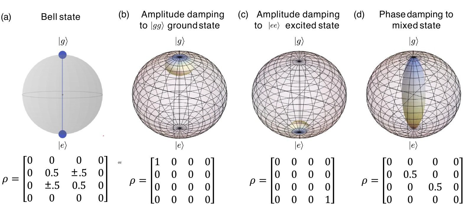
Figure 2: Bloch sphere representations of the 4 possible outcomes of a trial of our Monte-Carlo model, along with the associated density matrices. (a) The Bell state $|\Psi^{\pm}\rangle$. (b) Amplitude damping channel to the $|gg\rangle$ state deriving from transduced added noise photons. (c) Generalized amplitude damping to the excited state $|ee\rangle$ due to double excitation errors. (d) Phase damping channel to the $\rho_{mixed}=\frac{1}{2}(\ket{ge}\bra{ge}+\ket{eg}\bra{eg}$) state, showing loss of coherence from system without loss of energy.

After each heralding event, the fidelity of the resulting density matrix to the target state is calculated. The fidelity is calculated by using

$$F_{ic}=Tr[\rho^{{}^{\prime}}|\Psi^{+}\rangle\langle\Psi^{+}|]$$ (11)

where $\rho^{\prime}$ represents the density matrix after rotating into $|\Psi^{+}\rangle$. A full derivation of the single-click protocol’s density matrix is available in the appendix D.

Many trials are run, and the fidelity is averaged across these trials. The ebit rate is calculated by multiplying the attempt frequency by the Bell pair success fraction. For the 2-click and distillation protocols, additional heralding attempts are made, as prescribed by those protocols. Optimal protocols are then identified by adjusting the several parameters that can be used to trade off fidelity and ebit rate:

• The protocol type (e.g. 1-click, 2-click, EPL, or another distillation protocol).

• The parameter $p_{e}$.

• The transducer’s pump laser power or pulse time, which affect both $\eta$ and $N_{add}$.

The assumptions made in this simulation are as follows:

1. The superconducting qubit gates are ideal.

2. Superconducting qubit measurement fidelities are ideal.

3. The qubits’ relaxation and decoherence are disregarded (except when memory $T_{1}$ loss is explicitly included in Fig. 6).

4. The heralded states correspond to the density matrices as shown in  Fig. 2. In particular, the added noise process happens independently of the process of transduction of photons deriving from the superconducting qubits.

5. The noise photons obey Poissonian statistics.

6. The detector dark count rates are negligible compared to the rate of upconverted noise photons.

7. Parametric amplification effects are neglected, i.e. the transducers here are functioning solely as microwave-to-optical upconversion devices.

8. The product of the transducer’s pulse time and its bandwidth is 1, leading to an optimal amount of introduced added noise, given the specification of the transducer.

9. The single photon detectors are not photon-number resolving, i.e. they click if one or more photons reaches them within a time bin.

IV Results and Discussion

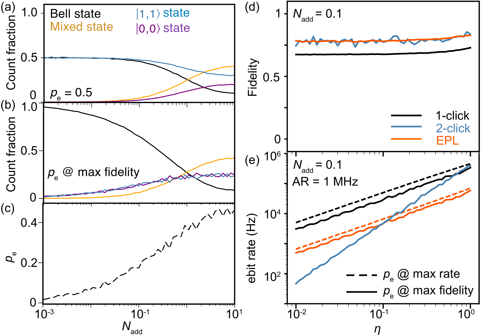
Figure 3: The fraction of heralded events corresponding to the scenarios shown in Fig. 2 at (a) $p_{e}=0.5$ and (b) the $p_{e}$ value that maximizes fidelity of the 1-click protocol. (c) The $p_{e}$ value that maximizes the fidelity of the 1-click protocol. (d) The fidelity and (e) ebit rate of the 1-click, 2-click and EPL protocols as a function of $\eta$, with $N_{add}$ = 0.1 and the attempt rate = 1 MHz.

In executing our Monte Carlo simulation, we generally average 5000 trials for each set of parameters.

We start by quantifying the count rate of the noise-induced errors during the 1-click remote entanglement process (Fig. 3(a,b)). The fraction of counts resulting in the desired Bell pair state increases as $N_{add}$ decreases, but this fraction saturates at 0.5 if $p_{e}$ is held constant. This saturation derives from double excitation errors. At $p_{e}=0.5$, the ebit rate for the 1-click and 2-click protocols is maximized, as is the fidelity of the 2-click protocol.

However, the $p_{e}$ value that maximizes fidelity for the 1-click rate depends on $N_{add}$ (Fig. 3(c)). When $N_{add}$ is high, the optimal $p_{e}$ value is high as well, so that the qubit excitation rate can compete with the noise photon rate. As $N_{add}$ is decreased, the optimal $p_{e}$ decreases as well, to minimize double excitation errors.

The simulated fidelity and ebit rate show several clear trends as $\eta$ is swept. The fidelity is fairly insensitive to $\eta$ (Fig. 3(d)). The 2-click and EPL fidelities exceed the 1-click fidelity and are nearly identical to each other. Naturally, the ebit rate is highly sensitive to $\eta$. The 2-click ebit rate scales quadratically with $\eta$, whereas the ebit rate for the 1-click and EPL protocols scales linearly with $\eta$ (Fig. 3(e)).

This difference in scaling between the 2-click protocol and the ebit protocol demonstrates the advantage of distillation. This difference derives from the use of the memory in distillation. With the 2-click protocol, two successful transduction events must happen in a row – hence the $\eta^{2}$ scaling. With the EPL protocol, the second transduction cycle can be attempted many times in a row, within the limits of the memory’s $T_{1}$ and $T_{2}$ times, so a linear scaling with $\eta$ is achieved. The EPL protocol’s benefit is that it allows for a 2-click-like fidelity with a 1-click-like ebit-rate scaling.

Fidelity is a strong function of $N_{add}$ (Fig. 4(a-c)). At very high $N_{add}$, the two-qubit fidelity approaches 0.25, the fidelity that is expected if each qubit’s state derives from a coin flip. As $N_{add}$ is decreased, the optimized 1-click fidelity reaches 90% at $N_{add}=10^{-2}$. However, the ebit rate for the fidelity-optimized 1-click protocol drops precipitously as $N_{add}$ is lowered, because the optimal $p_{e}$ value decreases with $N_{add}$ (Fig. 4(c)).

On the other hand, the EPL fidelity is insensitive to $p_{e}$ (Fig. 4(d)). Moreover, the fidelities for both the 2-click protocol and the EPL distillation protocols improve much faster than the 1-click fidelity as $N_{add}$ is lowered (Fig. 4(e). They reach 0.997 at $N_{add}$ = $10^{-3}$, corresponding to over an order of magnitude improvement (in infidelity) over the 1-click protocol. The EPL ebit-rate is maximized at $p_{e}$ = 0.3 (Fig. 4(f). The ebit rate for all three protocols is insensitive to $N_{add}$ until $N_{add}$ exceeds a threshold. This threshold is $N_{add}\sim 1$ for the 1-click protocol and $N_{add}\sim 0.1$ for the 2-click and EPL protocols (Fig. 4(c,f).

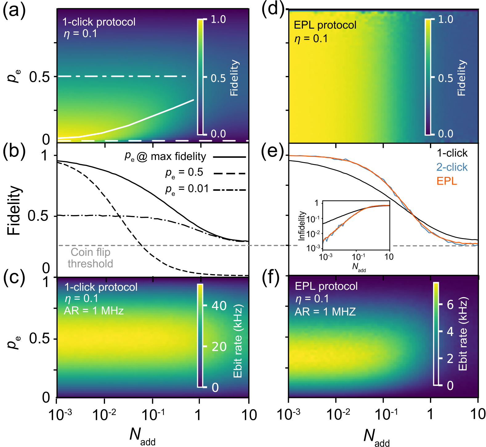
Figure 4: The fidelity and e-bit rate as a function of $N_{add}$. (a) The fidelity of the 1-click protocol as a function of $N_{add}$ and $p_{e}$, with $\eta$ = 0.1. The solid white line corresponds to maximum fidelity line cut. (b) Fidelity vs. $N_{add}$ line-cuts of (a) at maximum fidelity (solid line), maximum e-bit rate (dashed-dotted line), and minimal near-0 values of $p_{e}$ (dashed line). (c) E-bit rate as a function $N_{add}$ and $p_{e}$, with the attempt rate (AR) = 1 MHz. (d) Fidelity of the EPL protocol as a function of $N_{add}$ and $p_{e}$, with $\eta$ = 0.1. (e) Fidelity and infidelity of the 1-click, 2-click, and EPL protocols as a function of $N_{add}$ , with $p_{e}$ chosen to maximize fidelity for the 1-click protocol. (f) Ebit rate of the EPL protocol, with AR = 1 MHz, as before.

To understand how these variables interrelate, we consider a scenario in which both $\eta$ and $N_{add}$ are directly proportional to the laser pump power and then vary that power while fixing their ratio to $\eta/N_{add}=10$. We can then plot fidelity vs. ebit rate and identify outperforming protocols (Fig. 5). We find that for low ebit rates (below 10 kHz), the EPL protocol outperforms the 2-click protocol, whereas the 2-click protocol outperforms in the high $\eta$ regime when the ebit rate is above 10 kHz. We also plotted the performance of the Chi 3-to-1 distillation protocol [17] here, but it was not found to be optimal in any regime here.

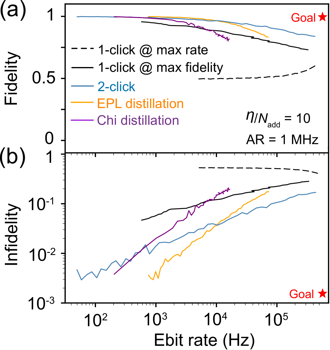
Figure 5: A comparison of e-bit rate vs. (a) fidelity and (b) infidelity for the 1-click, 2-click, EPL 2-to-1 distillation, and Chi 3-to-1 distillation protocols. To generate these curves, we vary $N_{add}$ (from $10^{-3}$ to $10^{-1}$) and $\eta$ (from $10^{-2}$ to 1) together, while fixing the ratio $\eta/N_{add}=10$, and setting the attempt rate to 1 MHz. For the 1-click protocol, $p_{e}$ can be chosen to maximize either fidelity or ebit rate.

We have not yet considered the effect of $T_{1}$ or $T_{2}$ decay of the first Bell pair while waiting for the second Bell pair to be heralded[38, 39]. With present-day transducers and superconducting qubits as memories, this decay is a significant consideration. Accordingly, we also modeled distillation in the presence of qubit relaxation. To be realistic, we started with present-day performance parameters given by the current generation of optomechanical transducers [9, 3, 40, 41, 42] and specified $\eta=10^{-4}$ , $N_{add}=0.5$, and a repetition rate of 100 kHz. We modeled the superconducting qubits as having $T_{1}=300$ $\mu s$, which is typical of high-performing transmons  [43, 44]. We find that distillation is not possible with present-day transducers, unless a quantum memory is used that has a significantly longer lifetime than that of a superconducting qubit.

However, the 1-click protocol comprising devices performing at these levels should be at the threshold of being able to demonstrate remote entanglement above 50% (Fig. 6). We also considered three improvement scenarios (S1, S2, and S3) and observe that as the transducer and $T_{1}$ performance metrics improve, distillation becomes viable. In improvement scenario S2 (Fig. 6), achieving a distilled fidelity of 0.97 at an ebit rate of 7.5 kHz requires a 1000$\times$ increase in $\eta$, and 50$\times$ reduction to $N_{add}$, as well as repetition rate improvements. In scenario S3, consisting of $\eta=0.3$, $N_{add}=0.001$, $T_{1}=10$ ms, and a repetition rate of 1 MHz, a Bell-pair fidelity of 0.997 and ebit rates exceeding 100 kHz are achievable. These results underscore the critical role of reducing noise and increasing transducer efficiency [18], along with reducing other insertion losses in the optical path.

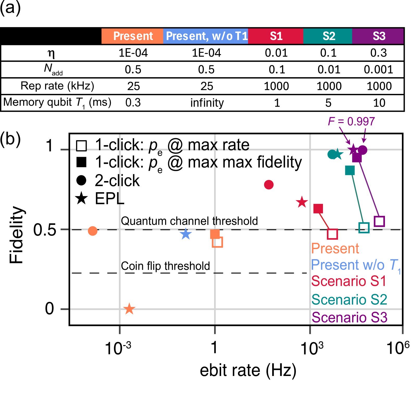
Figure 6: A comparison of ebit rate and fidelity for the 1-click, 2-click, and EPL protocols under five different scenarios. ”Present” is the approximate state-of-the-art. ”Present w/o $T_{1}$” is the same specifications except the memory qubit’s $T_{1}$ time is set to be infinity. For this scenario, only the EPL protocol’s metrics are shown, as the others do not use a memory. S1-S3 are three improvement scenarios. The solid lines connecting the open and closed squares represent points on the fidelity vs. ebit rate that can be achieved by the 1-click protocol through the choice of $p_{e}$.

Besides the simple distillation schemes considered here, there are other distillation schemes that could be implemented. Other 2-to-1 distillation schemes [22, 31] could be considered, or the distillation schemes considered here could be applied recursively. More sophisticated distillation protocols include hashing protocols, breeding protocols, stabilizer protocols, and many others [45, 18]. Furthermore, the output of Bell pairs generated by the 2-click protocol could be used as input states to any of these distillation schemes. In general, though, selecting the appropriate distillation protocol will involve a decision regarding how to trade off fidelity and ebit rate, and the EPL protocol already performs well with a low overhead. In the context of distilling Bell pairs heralded through transducers, another question is when multiple transducers per qubit should be considered. This would certainly help with the ebit rate and/or enable more advanced distillation protocols than simple 2-to-1 protocols. Because every transducer comes with a power, space, and wiring overhead, this approach could be impractical. Nonetheless, it should be considered if the number of required system-to-system links is low.

V Conclusion

Our analysis shows that present-day transducers are nearing the threshold of being capable of distributing Bell states with fidelities of 50%, a milestone for remote entanglement generation [1, 27]. The EPL protocol is a particularly promising distillation protocol, correcting both $\ket{gg}$ and $\ket{ee}$ errors and providing first-order protection against phase fluctuations caused by path-length differences [19]. Its fidelity matches that of the 2-click protocol across a wide parameter range, yet its ebit rate scales linearly with $\eta$.

However, for transducers to rival the performance of current all-microwave links with fidelities exceeding 90% [21, 22, 46], significant advances to transducer hardware are still needed. Distillation with today’s transducers and quantum memories comprising today’s superconducting qubits remains infeasible, as the memory dephasing rate exceeds the ebit rate.

Nonetheless, the application of entanglement distillation to remote entanglement of superconducting qubits has a clear pathway forward. As transducer device progress is realized, the improvement scenarios we considered show that high fidelities are possible. Alternatively, quantum memories such as the silicon-vacancy color center could mitigate decoherence and relaxation of the quantum memory [32]. Additionally, the use of hybrid quantum architectures that combine solid-state memories with photonic systems [27, 31] could address current limitations in transducer efficiency and noise. Together, these advances could enable advanced error-correction methods and entanglement distillation to provide a robust framework for long-distance quantum communication in noisy environments.

Data and Code Availability

The data and code that support the findings of this study are available from the corresponding authors upon reasonable request.

Appendix A Model for entanglement formation with transducers

An analytical model to describe transducer-mediated conditional entanglement of remote qubits has been previously devised [23], where the output from two qubits would be converted to optical frequencies via transduction and subsequently interfere the signals on a beam splitter. A click in one of the detectors is an indication that the single-click scheme has succeeded. Subsequently applying a symmetric $\pi$-pulse to the qubits and conditioning on a second click in a 2-click scheme decreases the sensitivity to transduced noise photons. The focus of this appendix is to compare the analytical calculation of fidelity and compare it with our Monte Carlo simulation.

The analytical derivation starts with understanding the constituents of the remote entanglement procedure, which are the transduction + optical path efficiency ($\eta$) and the dark count rate ($P_{d}$). The transduction efficiency $\eta$ of the transducer can be modeled as:

$$\eta=\eta_{h}\int_{0}^{T}|h_{out}(t)|^{2}dt$$ (12)

where $\eta_{h}=\int_{-\infty}^{\infty}\eta(\Omega)|h_{in}(\Omega)|^{2}d\Omega$ is the mode-dependent efficiency and $h_{out}$ is the outgoing signal from the transducer in a time interval $T$. Each transducer contributes an average dark count rate of $\frac{r_{N}T}{2}$ in each detector, where $r_{N}$ is the added noise rate, whereby the probability for at least one dark count in a particular detector is:

$$P_{d} =(1-e^{\frac{-r_{N}T}{2}})^{2}=(1-e^{-r_{N}T})$$ (13)

$$\approx(1-1+r_{N}T+O(r_{N}T)^{2})\approx r_{N}T$$

for $r_{N}T\ll 1$. Following the description from subsection II.1, we consider the various possible outcomes compatible with the fulfillment of the condition that a click occurs. This results in $\rho_{1-click}^{\prime}=\ket{\Psi}\bra{\Psi}$, the density matrix after the protocol, we obtain:

$$\rho_{1-click}^{{}^{\prime}} =\frac{1}{N_{1}}((1-P_{e})^{2}2P_{d}(1-P_{d})|00\rangle\langle 00|$$ (14)

$$+2P_{e}(1-P_{e})\eta(1-P_{d})|\Psi_{+}\rangle\langle\Psi_{+}|$$

$$+P_{e}(1-P_{e})(1-\eta)(1-P_{d})2P_{d}(|01\rangle\langle 01|+|10\rangle\langle 10|)$$

$$+P_{e}^{2}((1-(1-\eta)^{2})+(1-\eta)^{2}2P_{d})(1-P_{d})|11\rangle\langle 11|$$

where $N_{1}$ is the normalization factor and the relation holds $Tr[\rho_{1-click}^{{}^{\prime}}]=1$. $P_{e}$ represents the excitation probability of the superconducting qubits while $P_{d}$ represents the dark photon rate stemming from the noise rate given by the transducer and its efficiency $\eta$.

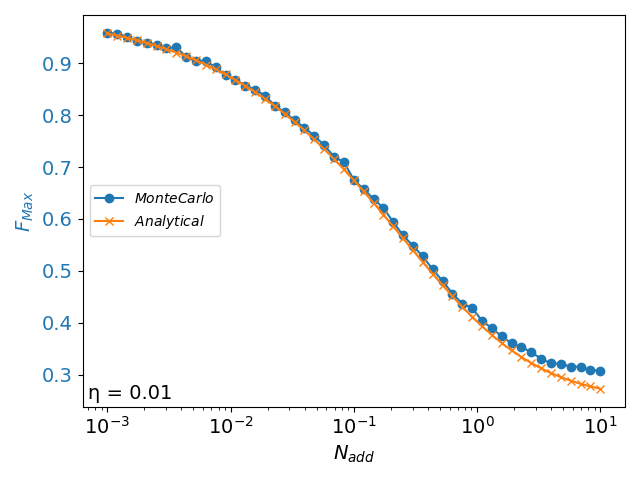
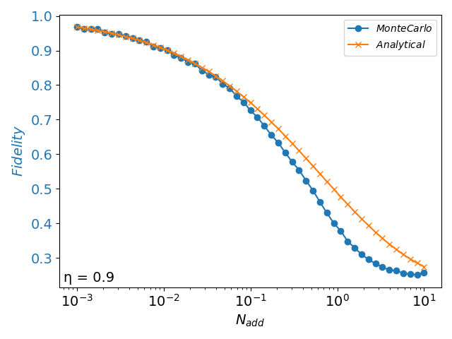
Figure 7: Fidelity for corresponding added noise $N_{add}$ at maximized excitation value $P_{e}$ for analytical [23] and numerical results. Left shows the evolution of the fidelity for a transducer efficiency $\eta=0.01$, the analytical and numerical agree almost perfectly wth the exception at larger $N_{add}$, where the analytical solutions starts to decay quickly to 0.25. Right Same results for $\eta=0.9$ where the results still agree well with small deviations.

An analytical result to the fidelity of the single click protocol can be derived by plugging equation 14 into equation 11. Under the assumption that the conditions in the limit of $\frac{P_{d}}{\eta}<<P_{e}<<1$, we obtain:

$$F_{1c}=\frac{2P_{e}(1-P_{e})\eta+P_{e}(1-P_{e})(1-\eta)2P_{d}}{P_{e}\eta(1-2P_{d})(2-P_{e}\eta)+2P_{d}}$$ (15)

From 15, we compare the analytical and numerical results in Fig. 7 for $\eta=0.01$ and $\eta=0.9$. In both cases, $p_{e}$ is optimized for fidelity. We observe that the analytical result [23] and numerical results agree well when $\eta=0.01$ and $N_{add}<1$. The divergences in the high $\eta$ / high $N_{add}$ regimes are due to discrepancies in the treatment of multiphoton events. It is important to note that the probability of having a dark count at a single detector is $r_{N}T$, but having a dark count in either detector is $2r_{N}T$.

The 2-click scheme follows similar definitions as the 1-click scheme. The scheme works in two steps, and we will take as a condition that at least 1-click in exactly one arm occurs in each of the two steps. This results in $\rho_{2-click}^{\prime}=\ket{\Psi}\bra{\Psi}$, the density matrix after the two-click protocol, we obtain:

$$\rho_{2-click}^{{}^{\prime}} =\frac{1}{N_{2}}((1-P_{e})^{2}2P_{d}(1-P_{d})([1-(1-\eta)^{2}](1-P_{d})+(1-\eta)^{2}2P_{d}(1-P_{d}))|00\rangle\langle 00|$$ (16)

$$+2P_{e}(1-P_{e})\eta^{2}(1-P_{d})^{2}|\Psi_{+}\rangle\langle\Psi_{+}|$$

$$+((\eta(1-P_{d})+(1-\eta)(1-P_{d})2P_{d})^{2}-\eta^{2}(1-P_{d})^{2})(|01\rangle\langle 01|+|10\rangle\langle 10|)$$

$$+P_{e}^{2}((1-(1-\eta)^{2})+(1-\eta)^{2}2P_{d})(1-P_{d})^{2}2P_{d}|11\rangle\langle 11|)$$

From the equations 14 and 16 it is clear that the two-photon scheme has a smaller sensitivity to added noise than the one-photon scheme. On the other hand, the two-photon scheme will have a lower success probability if the transducer has a low efficiency since it requires the detection of two photons.

Appendix B State of the Art Performance in Current Experimental Setups

	Bulk LiNbO3 [47]	Thin-Film LiNbO3 [48]	SiN membrane [49]	Si/ LiNbO3 P-O-M [11]	Si / LiNbO3 P-O-M [9]	Si O-M [50]
$\eta$	8.7%	0.9%	47%	$5.2\times 10^{-5}$	5%	0.47%
$N_{add}$	0.16	0.12	3.2	6	5	0.58
$f_{\text{rep}}$ (kHz)	0.5	CW	CW	100	170	CW
BW (MHz)	10	30	0.012	14.8	1.5	18

Table 1: Device performance parameters of several state-of-the-art transduction platforms.

Table 1 is a non-exhaustive list of the performance parameters of the current generation of high-performing quantum transducers. The following key parameters are included: transducer efficiency ($\eta$), added noise ($N_{add}$), operating frequency ($f_{rep}$), and bandwidth (BW). The platforms considered include LiNbO₃ electro-optics, LiNbO₃ piezo-optomechanics (P-O-M), and SiN membranes. Note that in this table, $\eta$ is the microwave waveguide to optical waveguide efficiency, not the end-to-end optical + transduction efficiency as in the rest of the paper. The latter includes not only transduction efficiency, but also fiber coupling efficiency, optical filter efficiencies, and detector efficiencies.

Appendix C Chi-Protocol Circuit Diagram

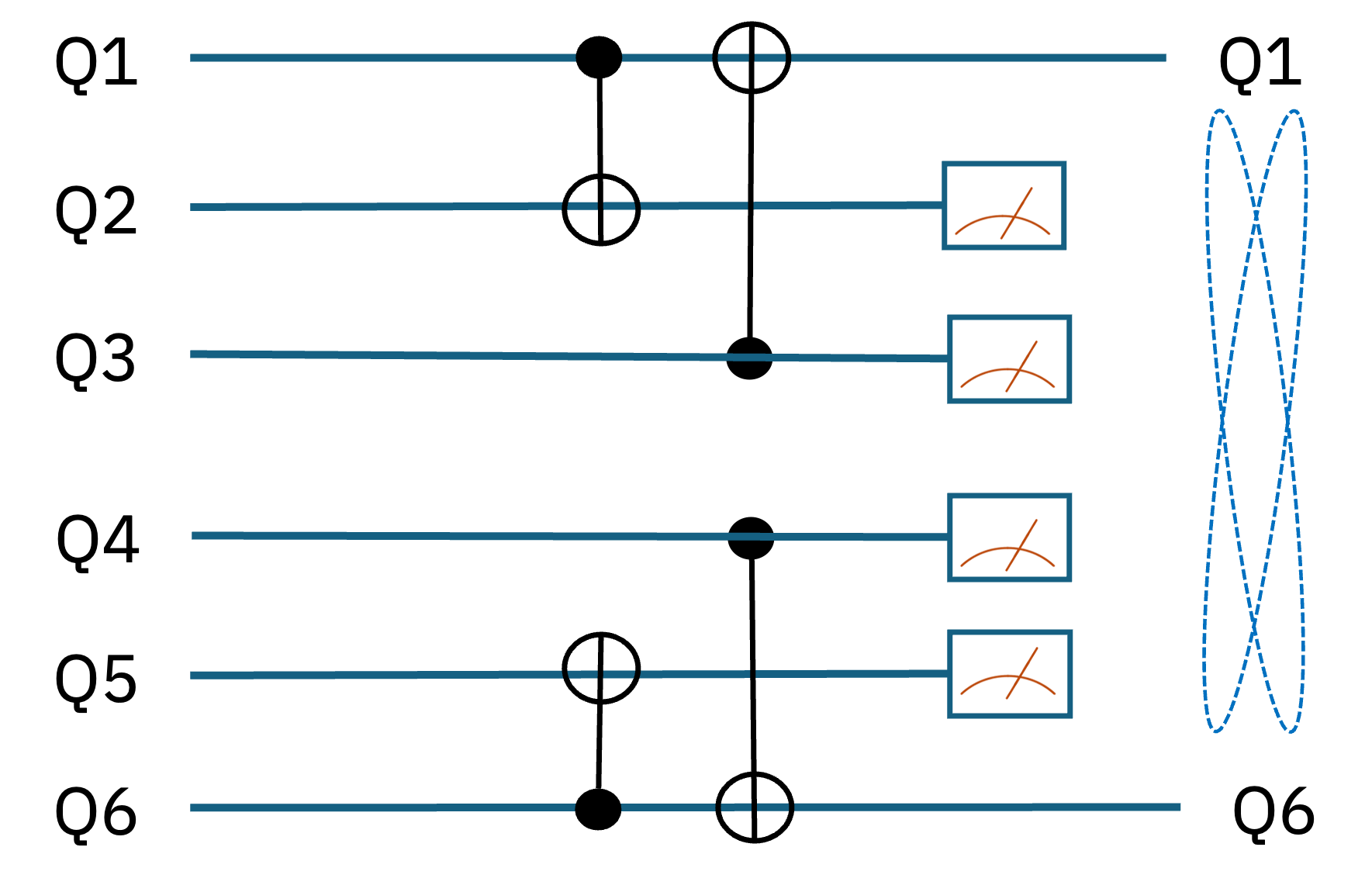
Figure 8: Chi protocol with local unitary operations $U_{A}$ and $U_{B}$ [17]

Fig. 8 displays the circuit diagram of the Chi protocol. This entanglement purification protocol works on three copies of a state via two bilateral controlled-NOT operations. The one-round success probability of the protocol is larger than 2-to-1 protocols, but comes with the added constraint of having to prepare three different copies of Bell pairs.

Appendix D Derivation of local phase stability via EPL Protocol

We initialize each of our two remote qubits into the superposition state $\frac{1}{\sqrt{2}}(|g\rangle+|e\rangle)$. Both qubits are excited and routed through the transducer where the upconverted photons are then collected and sent through a beam splitter prior to detection. If a photon is detected, then we obtain:

$$\rho=(1-N)|\Psi\rangle\langle\Psi|+N|ee\rangle\langle ee|$$ (17)

where $|\Psi\rangle=\frac{1}{\sqrt{2}}(|ge\rangle+e^{i\phi}|eg\rangle$. The local phase $\phi$ is introduced through optical path length fluctuations and can . When applying the EPL protocol for entanglement distillation we are able to remove such local phase. Starting with two noisy entangled pairs, each of the form $\rho$ , we apply bilocal CNOT gates within each cell according to the Fig. 1 circuit. The protocol then calls for one of the qubit pairs to be measured in the z basis. Any result other than “11” is rejected. Thus, measuring “11” implies that the remaining qubit pair is state $|\Psi\rangle$ and we have eliminated both the $|ee\rangle$ components due to photon loss and the unwanted phase $\phi$. We demonstrate the analysis with a more general approach also looking at mixed states and the $|gg\rangle$ state. Thus we start with noisy entangled pairs of the form:

$$\rho_{1}=N|\Psi\rangle\langle\Psi|+(1-N)(|gg\rangle\langle gg|+|ee\rangle\langle ee|)$$ (18)

and of the form

$$\rho_{2}=N|\Psi\rangle\langle\Psi|+(1-N)|M\rangle\langle M|$$ (19)

where $|M\rangle\langle M|=|ge\rangle\langle ge|+|eg\rangle\langle eg|$ and $\Psi$ as previously stated. The full density matrix is $\rho_{total}^{1}=\rho_{1}\otimes\rho_{1}$ and $\rho_{total}^{2}=\rho_{2}\otimes\rho_{2}$ such that

$$\rho_{total}^{1} =(N|\Psi\rangle\langle\Psi|+(1-N)(|gg\rangle\langle gg|+|ee\rangle\langle ee|))\otimes$$ (20)

$$(K|\Psi\rangle\langle\Psi|+(1-K)(|gg\rangle\langle gg|+|ee\rangle\langle ee|))$$

and

$$\rho_{total}^{2} =(N|\Psi\rangle\langle\Psi|+(1-N)(|M\rangle\langle M|))\otimes$$ (21)

$$(K|\Psi\rangle\langle\Psi|+(1-K)(|M\rangle\langle M|))$$

From there we extend and obtain:

$$\rho_{total}^{1} =NK(|\Psi\rangle|\Psi\rangle\langle\Psi|\langle\Psi|)+N(1-K)(|\Psi\rangle|gg\rangle\langle gg|\langle\Psi|+|\Psi\rangle|ee\rangle\langle ee|\langle\Psi|)$$ (22)

$$+K(1-N)(|gg\rangle|\Psi\rangle\langle\Psi|\langle gg|+|ee\rangle|\Psi\rangle\langle\Psi|\langle ee|)$$

$$+(1-K)(1-N)(|gg\rangle|gg\rangle\langle gg|\langle gg|+|gg\rangle|ee\rangle\langle ee|\langle gg|+|ee\rangle|gg\rangle\langle gg|\langle ee|+|ee\rangle|ee\rangle\langle ee|\langle ee|)$$

and

$$\rho_{total}^{2} =NK(|\Psi\rangle|\Psi\rangle\langle\Psi|\langle\Psi|)+N(1-K)(|\Psi\rangle|ge\rangle\langle ge|\langle\Psi|+|\Psi\rangle|eg\rangle\langle eg|\langle\Psi|)$$ (23)

$$+K(1-N)(|ge\rangle|\Psi\rangle\langle\Psi|\langle ge|+|eg\rangle|\Psi\rangle\langle\Psi|\langle eg|)$$

$$+(1-K)(1-N)(|ge\rangle|ge\rangle\langle ge|\langle ge|+|ge\rangle|eg\rangle\langle eg|\langle ge|)+|eg\rangle|ge\rangle\langle ge|\langle eg|+|eg\rangle|eg\rangle\langle eg|\langle eg|)$$

We apply then the bilocal CNOT gates such that $CNOT\rho_{total}CNOT^{\dagger}$ is:

$$\rho_{total}^{1} =NK(|ge\rangle(|gg\rangle+e^{i\phi}|ee\rangle)+|eg\rangle(|ee\rangle+e^{i\phi}|gg\rangle)((\langle gg|e^{-i\phi}+\langle ee|)e^{-i\phi}\langle eg|+(\langle gg|+\langle ee|e^{-i\phi})\langle ge|)$$ (24)

$$+N(1-K)(|ge\rangle|ge\rangle\langle ge|\langle ge|+e^{i\phi}|eg\rangle|eg\rangle\langle eg|\langle eg|e^{-i\phi})(|ge\rangle|eg\rangle\langle eg|\langle ge|+e^{i\phi}|eg\rangle|ge\rangle\langle ge|\langle eg|e^{-i\phi})$$

$$+K(1-N)(|gg\rangle(|ge\rangle+e^{i\phi}|eg\rangle)(\langle eg|e^{-i\phi}+\langle ge|)\langle gg|+|ee\rangle(|eg\rangle+e^{i\phi}|ge\rangle)(\langle ge|e^{-i\phi}+\langle eg|)\langle ee|)$$

$$+(1-K)(1-N)(|gg\rangle|gg\rangle\langle gg|\langle gg|+|gg\rangle|ee\rangle\langle ee|\langle gg|+|ee\rangle|ee\rangle\langle ee|\langle ee|+|ee\rangle|gg\rangle\langle gg|\langle ee|)$$

and

$$\rho_{total}^{2} =NK(|ge\rangle(|gg\rangle+e^{i\phi}|ee\rangle)+|eg\rangle(|ee\rangle+e^{i\phi}|gg\rangle)((\langle gg|e^{-i\phi}+\langle ee|)e^{-i\phi}\langle eg|+(\langle gg|+\langle ee|e^{-i\phi})\langle ge|)$$ (25)

$$+N(1-K)(|ge\rangle|gg\rangle\langle gg|\langle ge|+e^{i\phi}|eg\rangle|ee\rangle\langle ee|\langle eg|e^{-i\phi})(|ge\rangle|ee\rangle\langle ee|\langle ge|+e^{i\phi}|eg\rangle|gg\rangle\langle gg|\langle eg|e^{-i\phi})$$

$$+K(1-N)(|ge\rangle|gg\rangle\langle gg|\langle ge|+e^{i\phi}|ge\rangle|ee\rangle\langle ee|\langle ge|e^{-i\phi})+|eg\rangle|ee\rangle\langle ee|\langle eg|+e^{i\phi}|eg\rangle|gg\rangle\langle gg|\langle eg|e^{-i\phi})$$

$$+(1-K)(1-N)(|ge\rangle|gg\rangle\langle gg|\langle ge|+|ge\rangle|ee\rangle\langle ee|\langle ge|+|eg\rangle|ee\rangle\langle ee|\langle eg|+|eg\rangle|gg\rangle\langle gg|\langle eg|)$$

We now rearrange and collect terms to measure the target qubits:

$$\rho_{total}^{1} =NK((|ge\rangle+e^{2i\phi}|eg\rangle)|gg\rangle\langle gg|(\langle ge|+\langle eg|e^{-2i\phi})$$ (26)

$$+e^{i\phi}(|eg\rangle+|ge\rangle)\textbf{$|ee\rangle\langle ee|$}(\langle ge|+\langle eg|)e^{-i\phi}((\langle gg|e^{-i\phi}+\langle ee|)e^{-i\phi}\langle eg|+(\langle gg|+\langle ee|e^{-i\phi})\langle ge|))$$

$$+N(1-K)((|ge\rangle+eg\rangle)|\textbf{$|ge\rangle\langle ge|$}(\langle eg|+\langle ge|)+e^{i\phi}(|eg\rangle+|ge\rangle)\textbf{$|eg\rangle\langle eg|$}(\langle eg|+\langle ge|)e^{-i\phi})$$

$$+K(1-N)((|gg\rangle+e^{i\phi}|ee\rangle)\textbf{$|ge\rangle\langle ge|$}(\langle ee|e^{-i\phi}+\langle gg|)+(|ee\rangle+e^{i\phi}|gg\rangle)\textbf{$|eg\rangle\langle eg|$}(\langle gg|e^{-i\phi}+\langle ee|))$$

$$+(1-K)(1-N)((|gg\rangle+|ee\rangle)\textbf{$|gg\rangle\langle gg|$}(\langle gg|+\langle ee|)+(|gg\rangle+|ee\rangle)\textbf{$|ee\rangle\langle ee|$}(\langle gg|+\langle ee|))$$

and

$$\rho_{total}^{2} =NK((|ge\rangle+e^{2i\phi}|eg\rangle)|gg\rangle\langle gg|(\langle ge|+\langle eg|e^{-2i\phi})$$ (27)

$$+e^{i\phi}(|eg\rangle+|ge\rangle)|ee\rangle\langle ee|(\langle ge|+\langle eg|)e^{-i\phi}((\langle gg|e^{-i\phi}+\langle ee|)e^{-i\phi}\langle eg|+(\langle gg|+\langle ee|e^{-i\phi})\langle ge|))$$

$$+(N+K-2NK)((|ge\rangle+e^{i\phi}eg\rangle)||gg\rangle\langle gg|(\langle eg|e^{-i\phi}+\langle ge|)+(|ge\rangle+e^{i\phi}|eg\rangle)|ee\rangle\langle ee|(\langle eg|e^{-i\phi}+\langle ge|)$$

$$+(1-K)(1-N)((|ge\rangle+|eg\rangle)|gg\rangle\langle gg|(\langle eg|+\langle ge|)+(|ge\rangle+|eg\rangle)|ee\rangle\langle ee|(\langle eg|+\langle ge|))$$

We measure only the target qubits with flag $|11\rangle$. We see that for the first configuration only two possible outcomes exist, while for the second configuration three possible outcomes exist, namely:

$$\rho_{total}^{1} =NK((|eg\rangle+|ge\rangle)\textbf{$|ee\rangle\langle ee|$}(\langle ge|+\langle eg|))+(1-K)(1-N)((|gg\rangle+|ee\rangle)\textbf{$|ee\rangle\langle ee|$}(\langle gg|+\langle ee|))$$ (28)

and

$$\rho_{total}^{2} =NK((|eg\rangle+|ge\rangle)|ee\rangle\langle ee|(\langle ge|+\langle eg|))+(N+K-2NK)((|ge\rangle+e^{i\phi}|eg\rangle)|ee\rangle\langle ee|(\langle eg|e^{-i\phi}+\langle ge|)$$ (29)

$$+(1-K)(1-N)((|ge\rangle+|eg\rangle)|ee\rangle\langle ee|(\langle eg|+\langle ge|))$$

For the first configuration, the unknown local phase $\phi$ is eliminated. Due to the generalization of the state with $|00\rangle$, the system may return the Bell state $\Phi$ in case of a double error configuration while preparing the initial Bell pairs. Thus, we state that the system is protected against local bit flips up to second order. For the other configuration when looking at the mixed state $|M\rangle$ we observe that the dependence on the local phase $\phi$ does only vanish for an ideal configuration where both states were initially prepared with an entangled state. Whereas interestingly, a double error configuration would lead to a correct result of $\Psi$.

References

- Zhong et al. [2018] C. Zhong, X. Han, and L. Jiang, Physical Review Applied 18, 032322 (2018).
- Zhao et al. [2023] H. Zhao, A. Bozkurt, and M. Mirhosseini, Optica 10, 790 (2023).
- Mirhosseini et al. [2020] M. Mirhosseini, A. Sipahigil, M. Kalaee, and O. Painter, Nature 588, 599 (2020).
- Wang et al. [2022a] C. Wang, I. Gonin, A. Grassellino, S. Kazakov, A. Romanenko, V. P. Yakovlev, and S. Zorzetti, npj Quantum Information 8, 149 (2022a).
- Kumar et al. [2023] A. Kumar, A. Suleymanzade, M. Stone, L. Taneja, A. Anferov, D. I. Schuster, and J. Simon, Nature 615, 614 (2023).
- Wang et al. [2022b] C.-H. Wang, F. Li, and L. Jiang, Nature Communications 13, 6698 (2022b).
- Weaver et al. [2023] M. J. Weaver, P. Duivestein, A. C. Bernasconi, S. Scharmer, M. Lemang, T. C. van Thiel, F. Hijazi, B. Hensen, S. Gröblacher, and R. Stockill, in European Quantum Electronics Conference (Optica Publishing Group, 2023) p. eb_13_2.
- Sahbaz et al. [2024] F. Sahbaz, J. N. Eckstein, D. J. Van Harlingen, and S. I. Bogdanov, Physical Review A 109, 042409 (2024).
- Jiang et al. [2020] W. Jiang, C. J. Sarabalis, Y. D. Dahmani, R. N. Patel, F. M. Mayor, T. P. McKenna, R. Van Laer, and A. H. Safavi-Naeini, Nature communications 11, 1166 (2020).
- Simonsen et al. [2019] A. Simonsen, S. A. Saarinen, J. D. Sanchez, J. H. Ardenkjær-Larsen, A. Schliesser, and E. S. Polzik, Optics Express 27, 18561 (2019).
- Weaver et al. [2024] M. J. Weaver, P. Duivestein, A. C. Bernasconi, S. Scharmer, M. Lemang, T. C. v. Thiel, F. Hijazi, B. Hensen, S. Gröblacher, and R. Stockill, Nature Nanotechnology 19, 166 (2024).
- Imamouglu [2009] A. Imamouglu, Physical review letters 102, 083602 (2009).
- Verdú et al. [2009] J. Verdú, H. Zoubi, C. Koller, J. Majer, H. Ritsch, and J. Schmiedmayer, Physical review letters 103, 043603 (2009).
- Shi and Zhuang [2024] H. Shi and Q. Zhuang, arXiv preprint 2404.09441 https://doi.org/10.48550/arXiv.2404.09441 (2024).
- Meesala et al. [2024] S. Meesala, D. Lake, S. Wood, P. Chiappina, C. Zhong, A. D. Beyer, M. D. Shaw, L. Jiang, and O. Painter, Physical Review X 14, 031055 (2024).
- Bennett et al. [1996] C. H. Bennett, G. Brassard, S. Popescu, B. Schumacher, J. A. Smolin, and W. K. Wootters, Physical review letters 76, 722 (1996).
- Chi et al. [2012] D. P. Chi, T. Kim, and S. Lee, Physics Letters A 376, 143 (2012).
- Rozpedek et al. [2018] F. Rozpedek, T. Schiet, L. P. Thinh, D. Elkouss, A. C. Doherty, and S. Wehner, Physical Review A 97, 062333 (2018).
- Nickerson et al. [2014] N. H. Nickerson, J. F. Fitzsimons, and S. C. Benjamin, Physical Review X 4, 041041 (2014).
- Beukers et al. [2024] H. K. Beukers, M. Pasini, H. Choi, D. Englund, R. Hanson, and J. Borregaard, PRX Quantum 5, 010202 (2024).
- Wu et al. [2024] X. Wu, H. Yan, G. Andersson, A. Anferov, M.-H. Chou, C. R. Conner, J. Grebel, Y. J. Joshi, S. Li, J. M. Miller, et al., Physical Review X 14, 041030 (2024).
- Zhao et al. [2021] X. Zhao, B. Zhao, Z. Wang, Z. Song, and X. Wang, npj Quantum Information 7, 159 (2021).
- Zeuthen et al. [2020] E. Zeuthen, A. Schliesser, A. S. Sørensen, and J. M. Taylor, Quantum Science and Technology 5, 034009 (2020).
- Cabrillo et al. [1999] C. Cabrillo, J. I. Cirac, P. Garcia-Fernandez, and P. Zoller, Physical Review A 59, 1025 (1999).
- Campbell and Benjamin [2008] E. T. Campbell and S. C. Benjamin, Physical review letters 101, 130502 (2008).
- Narla et al. [2016] A. Narla, S. Shankar, M. Hatridge, Z. Leghtas, K. M. Sliwa, E. Zalys-Geller, S. O. Mundhada, W. Pfaff, L. Frunzio, R. J. Schoelkopf, et al., Physical Review X 6, 031036 (2016).
- Kurokawa et al. [2022] H. Kurokawa, M. Yamamoto, Y. Sekiguchi, and H. Kosaka, Physical Review Applied 18, 064039 (2022).
- Barrett and Kok [2005] S. D. Barrett and P. Kok, Physical Review A—Atomic, Molecular, and Optical Physics 71, 060310 (2005).
- Deutsch et al. [1996] D. Deutsch, A. Ekert, R. Jozsa, C. Macchiavello, S. Popescu, , and A. Sanpera, Physical Review Letters 77, 2818 (1996).
- Dür et al. [1999] W. Dür, H.-J. Briegel, J. I. Cirac, and P. Zoller, Physical Review A 59, 169 (1999).
- Yan et al. [2022] H. Yan, Y. Zhong, H.-S. Chang, A. Bienfait, M.-H. Chou, C. R. Conner, É. Dumur, J. Grebel, R. G. Povey, and A. N. Cleland, Physical Review Letters 128, 080504 (2022).
- Knaut et al. [2024] C. Knaut, A. Suleymanzade, Y.-C. Wei, D. Assumpcao, P.-J. Stas, Y. Huan, B. Machielse, E. Knall, M. Sutula, G. Baranes, et al., Nature 629, 573 (2024).
- M [2010] T. M, Physical Review A 81, 063837 (2010).
- Pan et al. [1998] J.-W. Pan, D. Bouwmeester, H. Weinfurter, and A. Zeilinger, Physical review letters 80, 3891 (1998).
- Bernien et al. [2013] H. Bernien, B. Hensen, W. Pfaff, G. Koolstra, M. S. Blok, L. Robledo, T. H. Taminiau, M. Markham, D. J. Twitchen, L. Childress, et al., Nature 497, 86 (2013).
- Siddhu and Smolin [2023] V. Siddhu and J. Smolin, Physical Review A 108, 032617 (2023).
- Pal [2022] R. Pal, Physical Review A 97, 064039 (2022).
- Siddhu et al. [2024] V. Siddhu, D. Abedlahdi, J.-O. Tomas, and J. Smolin, arXiv preprint 4505.06231v1 https://doi.org/10.48550/arXiv.2405.06231 (2024).
- Aliferis et al. [2009] P. Aliferis, F. Brito, D. DiVincenzo, J. Preskill, M. Steffen, and B. Terhal, New J. Phys. 11, 013061 (2009).
- Han et al. [2021] X. Han, W. Fu, C.-L. Zou, L. Jiang, and H. X. Tang, Optica 8, 1050 (2021).
- Andrews et al. [2014] R. W. Andrews, R. W. Peterson, T. P. Purdy, K. Cicak, R. W. Simmonds, C. A. Regal, and K. W. Lehnert, Nature physics 10, 321 (2014).
- Fang et al. [2016] K. Fang, M. H. Matheny, X. Luan, and O. Painter, Nature Photonics 10, 489 (2016).
- Place et al. [2021] A. P. Place, L. V. Rodgers, P. Mundada, B. M. Smitham, M. Fitzpatrick, Z. Leng, A. Premkumar, J. Bryon, A. Vrajitoarea, S. Sussman, et al., Nature communications 12, 1779 (2021).
- Bal et al. [2024] M. Bal, A. A. Murthy, S. Zhu, F. Crisa, X. You, Z. Huang, T. Roy, J. Lee, D. v. Zanten, R. Pilipenko, et al., npj Quantum Information 10, 43 (2024).
- W.Dür and H.J.Briegel [2007] W.Dür and H.J.Briegel, IOP Science 70, 1381 (2007).
- Zhong et al. [2021] Y. Zhong, H.-S. Chang, A. Bienfait, É. Dumur, M.-H. Chou, C. R. Conner, J. Grebel, R. G. Povey, H. Yan, D. I. Schuster, et al., Nature 590, 571 (2021).
- Sahu et al. [2022] R. Sahu, W. Hease, A. Rueda, G. Arnold, L. Qiu, and J. M. Fink, Nature communications 13, 1276 (2022).
- Warner et al. [2023] H. K. Warner, J. Holzgrafe, B. Yankelevich, D. Barton, S. Poletto, C. Xin, N. Sinclair, D. Zhu, E. Sete, B. Langley, et al., arXiv preprint arXiv:2310.16155 https://doi.org/10.48550/arXiv.2310.16155 (2023).
- Brubaker et al. [2022] B. M. Brubaker, J. M. Kindem, M. D. Urmey, S. Mittal, R. D. Delaney, P. S. Burns, M. R. Vissers, K. W. Lehnert, and C. A. Regal, Physical Review X 12, 021062 (2022).
- Zhao et al. [2024] H. Zhao, W. D. Chen, A. Kejriwal, and M. Mirhosseini, arXiv preprint arXiv:2406.02704 https://doi.org/10.48550/arXiv.2406.02704 (2024).