On the Identifiability of Causal Abstractions
Xiusi Li Sékou-Oumar Kaba Siamak Ravanbakhsh
Mila, McGill University Mila, McGill University Mila, McGill University
Abstract
Causal representation learning (CRL) enhances machine learning models’ robustness and generalizability by learning structural causal models associated with data-generating processes. We focus on a family of CRL methods that uses contrastive data pairs in the observable space, generated before and after a random, unknown intervention, to identify the latent causal model. (Brehmer et al., , 2022) showed that this is indeed possible, given that all latent variables can be intervened on individually. However, this is a highly restrictive assumption in many systems. In this work, we instead assume interventions on arbitrary subsets of latent variables, which is more realistic. We introduce a theoretical framework that calculates the degree to which we can identify a causal model, given a set of possible interventions, up to an abstraction that describes the system at a higher level of granularity.
1 INTRODUCTION
Causal representation learning (CRL) (Schölkopf et al., , 2021) generalizes non-linear independent component analysis (Hyvärinen and Pajunen, , 1999; Hyvarinen et al., , 2019) and causal discovery (Spirtes et al., , 2001), aiming to extract both latent variables and their causal graph in the form of structural causal models (SCMs). The question of identifiability naturally arises since we would like to guarantee that the set of models consistent with the given observable distribution is unique up to some equivalence class. In particular, we would like to know the level of granularity at which the true latent variables and the causal graph can be recovered.
We consider the problem of CRL assuming we have access to counterfactual data pairs and from the same observable space, before and after a random, unknown intervention. This is necessitated by the infeasibility of learning disentangled representations from unsupervised observational data alone (Hyvärinen and Pajunen, , 1999; Locatello et al., , 2019), and is sometimes referred to as self-supervised (Von Kügelgen et al., , 2021), contrastive (Zimmermann et al., , 2021), or weakly supervised learning (Shu et al., , 2019; Locatello et al., , 2020; Brehmer et al., , 2022; Ahuja et al., , 2022).
Previously, in this particular setting, it has been shown that the full causal graph can be recovered up to isomorphism (Brehmer et al., , 2022), and all the latent variables can be recovered up to element-wise diffeomorphism. However, as was noted by the authors, this result relies on overly restrictive assumptions; for example, the number of nodes on the causal graph must be known in advance, and each node must be intervened upon individually with nonzero probability.
Instead, we show that when we remove these assumptions, we can still identify “coarser” versions of the causal model, known as its abstractions, the related works of which we will expand on in the following paragraph. This relaxation is significant as it makes the setting much more realistic; in many systems, intervening on every variable individually is infeasible.
Causal abstraction (Rubenstein et al., , 2017; Beckers and Halpern, , 2019; Rischel, , 2020; Rischel and Weichwald, , 2021; Otsuka and Saigo, , 2022; Anand et al., , 2023; Massidda et al., , 2023) is the study of how microscopic variables and causal mechanisms can be aggregated to macroscopic abstractions on a higher level while maintaining a notion of interventional consistency, which enables more efficient reasoning and interpretability (Geiger et al., , 2021, 2024). Since this is still an emerging avenue of research, a standard unified formalism has yet to be established. However, as was highlighted previously in (Zennaro, , 2022), all of the various definitions of causal abstractions, in one way or another, tend to have a structural map dealing with the causal graph, and a distributional map dealing with the variables and stochastic causal mechanisms associated with its nodes and edges respectively.
In classic causal inference, the idea of structural abstraction can in some sense already be found in the form of Markov equivalence classes, or interventional Markov equivalence classes (Verma and Pearl, , 1990; Hauser and Bühlmann, , 2012; Yang et al., , 2018), where in the simplest cases, directed edges on the causal graph are abstracted away to undirected ones.
In CRL, the concept of distributional abstraction is more prevalent. For example, (Von Kügelgen et al., , 2021) introduces a definition for block-identifiability, in which the grouping of latent variables into blocks essentially serves as an abstraction of individual latent variables. More recent works (Ahuja et al., , 2022; Yao et al., , 2023) also examine overlapping blocks of latent variables and the identifiability of their intersections, complements, and unions.
In this paper, we investigate the identifiability of latent causal models up to their abstractions. Previous works in this setting have either focused on the problem of whether a pre-conceived latent causal model can be identified at all (Brehmer et al., , 2022), or are only concerned with identifying abstractions of the latent variables without identifying abstractions of the latent causal graph (Von Kügelgen et al., , 2021; Ahuja et al., , 2022; Yao et al., , 2023).
To the best of our knowledge, we provide the first identifiability results that give a graphical criterion for the degree of abstraction which we can identify latent causal models up to, depending on the interventional data available within the context of the weakly-supervised CRL problem, which take into account both structural and distributional properties of SCMs.
We structure the remainder of this work as follows. In Section 2.1 we introduce the weakly-supervised CRL problem setup in terms of the data generating process, which is essentially the same as the one outlined in (Brehmer et al., , 2022). In Section 2.2, we proceed to give increasingly restrictive definitions of the identifiability of causal model parameters up to equivalence, and in Section 2.3 we move on to increasingly restrictive definitions of the identifiability of causal model parameters up to abstraction. In Section 3 we explain the assumptions behind our main results, before presenting the statements. We leave the detailed proofs of these results to the appendix but draw attention to some key properties of the data generating process in Section 3.3, and the proof techniques used at a high level. In Section 3.4 we provide some intuition for some of the unexpected conclusions that can be drawn from the results. Finally, in Section 4, we outline the various downstream applications of our results, as well their limitations.
2 PROBLEM FORMULATION
2.1 DATA GENERATING PROCESS
In this section, we describe the data-generating process in our problem setting, which is the functional relationship between the latent causal model parameters and the resultant distribution of counterfactual or contrastive pairs of observational data.
We first introduce the structural causal model (SCM) describing the pre-intervention latent variables. Let be a directed acyclic graph, and associate each of the nodes with a vector space , a random variable taking values on , as well as a conditional probability distribution . Furthermore, let each of the conditional distributions have a functional representation 111The functional characterization of causal mechanisms, as was first introduced in (Verma and Pearl, , 1990) allows us to define the effect of interventions on the model, and is sometimes referred to as noise outsourcing in contemporary literature (see e.g. Bloem-Reddy et al., (2020)).
| (1) |
where the distributions of the exogenous variables are all mutually independent, and each is a deterministic function. Then we can denote and , and define a deterministic function by successively applying the causal mechanisms . Therefore the distribution of the pre-intervention latents can be parametrized by
| (2) |
We next describe the interventions on the latent variables. Let be a random variable taking values in the power set of vertices of (assumed to be finite), which tells us which latent variables are intervened upon at any one time. We denote the distribution of this discrete random variable as . Futhermore we write and refer to its elements as intervention targets (i.e. the subsets of nodes which get intervened upon with nonzero probability). In the event that for some , we assume that for every node in the causal mechanism from to becomes completely severed, in what is known as a perfect intervention. Therefore, the post-intervention latents conditional on satisfy
| (3) |
| (4) |
where the new exogenous variable corresponding to the target set post-intervention is independent from the pre-intervention exogenous variable , and each is a new function. Thus we can describe the effect of a random, unknown intervention on the structural causal model. Therefore the joint distribution of pre-intervention and post-intervention latent pairs can be parametrized by , where
| (5) |
Finally, let be the vector space known as the observation space, and let be an invertible mixing function such that
| (6) |
Therefore the joint distribution of counterfactual pairs of observational data can be parametrized by
| (7) |
It is important to note that the counterfactual setting outlined here differs from methods using interventional data (Brouillard et al., , 2020; Gresele et al., , 2020; Ahuja et al., , 2023; von Kügelgen et al., , 2024; Zhang et al., , 2024) in two respects.
-
1.
The counterfactual setting makes the more restrictive assumption of having access to the joint distribution of , whereas the interventional setting usually only assumes access to the marginal distributions of and separately.
-
2.
The interventional setting makes the more restrictive assumption of being able to observe the type of intervention that occurs, even though the exact intervention target corresponding to a given type may be unknown. Concretely, in the interventional setting, we assume access to multiple marginal distributions of indexed by an environment222This is also sometimes referred to as a “view” Yao et al., (2023) variable . The crucial point here is that is observable, and that for any fixed , the latent variable is generated by a causal model with an invariant causal structure. In comparison, in the counterfactual setting, the intervention variable is not observable, and samples of are generated by a mixture of causal models with distinct graphical structures.
While CRL methods using interventional data are arguably more practical for applications such as biology (Belyaeva et al., , 2021), where we have access to data generated from known experimental settings; methods using counterfactuals are better suited to cases such as temporal data from dynamical systems or offline reinforcement learning (Lippe et al., , 2022; Ahuja et al., , 2022; Brehmer et al., , 2022), where at any given time step a random intervention may take place. Further justification for the assumption of availability of counterfactual data pairs will be elaborated on in Section 4.
2.2 IDENTIFIABILITY UP TO EQUIVALENCE
Identifiability in statistics refers to the ability to uniquely determine the true values of model parameters from observed data. A model is considered strongly identifiable if there is only a single set of parameter values that can generate the observed data. More generally, identifiability up to an equivalence class means that while there may be multiple sets of parameter values that can generate the same observed data, these sets are equivalent in some meaningful way.
For our purposes, we assume there exist some ground truth parameters , and that we may take unlimited samples from the latent causal model , in order to learn an estimator of . We say that is identifiable up to some equivalence relation with respect to some hypothesis class of model parameters , if for any
| (8) |
2.2.1 LATENT DISENTANGLEMENT
One instance of an equivalence relation between and is defined in terms of an equivalence relation between the corresponding mixing function and . It is known as disentanglement (Bengio et al., , 2013; Higgins et al., , 2018), and we will draw attention to two variants of its definition.
The first variant deals with a single latent subspace that we want to isolate, which loosely speaking means that we want any two equivalent models to produce latent distributions that have the same marginals when restricted to this subspace.
Definition 2.1 (Latent disentanglement).
Given latent causal models parametrized by and as defined in Section 2.1, and latent subspaces and , we say that
with respect to these subspaces, if there exists a measurable function such that if we define the random variables and to be the latent components of and corresponding to the latent subspace and respectively , then the function satisfies
| (9) |
Alternatively, we can say that the encoder disentangles the ground truth latent variable by identifying it with the variable in the resultant latent representation .
We emphasize that the above definition is a distributional equivalence between a single pair of latent components in two causal models, without placing constraints on any of the other components.
The second variant of the definition of disentanglement deals with a full decomposition of the latent space into a direct sum of latent subspaces, such that we want any two equivalent models to produce latent distributions that have the same marginals when restricted to any of the subspaces in this decomposition.
Definition 2.2 (Full latent disentanglement).
Given latent causal models parametrized by and as defined in Section 2.1, and latent space decompositions and , we say that
with respect to these decompositions, if there exist a bijective function and measurable functions for all such that if we define the random variables and to be the latent components of and corresponding to the latent subspaces and respectively, then for all we have
| (10) |
Alternatively, we can say that the encoder produces a fully disentangled representation of the ground truth latent variables .
We emphasize that the above definition consists of distributional equivalences between the full sets of latent components in two causal models, up to the permutation given by , therefore it is easy to check that the following statement holds.
Lemma 2.1.
Given latent causal models parametrized by and as defined in Section 2.1, suppose with respect to the decompositions and . Then for all , we have with respect to and .
2.2.2 STRUCTURAL CAUSAL MODEL ISOMORPHISM
Note that so far, we have only defined distributional equivalences between the variables of the latent causal model and their representations. An even stronger equivalence relation than full latent disentanglement between and takes causal structure into account, and requires that in addition the causal graphs and be isomorphic. This is sometimes referred to as structural causal model isomorphism (Fong, , 2013; Brehmer et al., , 2022) or the CRL identifiability class von Kügelgen et al., (2024).
Definition 2.3 (SCM isomorphism).
Given latent causal models parametrized by and as defined in Section 2.1, note that there exist canonical decompositions of their latent subspaces and into direct sums of subspaces and respectively. We say that
if there exists a graph isomorphism , and measurable functions such that Eq(10) holds for all .
Alternatively, we say that the structural causal models with parameters and are isomorphic.
Note that the above definition consists of a structural equivalence in the form of the graph isomorphism, as well as distributional equivalences between latent components in two causal models that are compatible with the graph isomorphism, therefore it is easy to check that the following statement holds.
Lemma 2.2.
Given latent causal models parametrized by and as defined in Section 2.1, suppose . Then with respect to and .
2.3 IDENTIFIABILITY UP TO ABSTRACTION
In this section, we introduce the concept of identifiability up to model abstraction, which can be thought of as the “common factor” between all models which are consistent with the observable distribution.
To do this, we need some notion of a partial order on , which compares causal models by their level of granularity or, in some sense, complexity. Broadly speaking, given any causal model , there is always another, more complex model that produces the same observable distribution 333For example, we can always add more “dummy variables” that increase the number of nodes on the causal graph, which, when marginalized upon do not produce any effect on the final observable distributions under intervention. What we want to know is what all the models which are able to produce the same observable distribution as have in common, meaning that we want to find an abstraction of that is the infimum of all these models. Note that this principle of finding minimal causal structures consistent with the observed data, which can be thought of as a reformulation of Occam’s razor, is discussed at length in Chapter 2 of Pearl, (2009).
Concretely, in our problem setting, is said to be identifiable up to the abstraction with respect to and some hypothesis class of parameters if for all
| (11) |
We will proceed to extend the definitions of equivalence relations on the parameter space from the previous subsection to (weak) partial orders on .
2.3.1 LATENT ABSTRACTION
Definition 2.4 (Latent abstraction).
Given latent causal models parametrized by and as defined in Section 2.1, and a latent subspace , together with a set of complementary latent subspaces , we say that
with respect to this latent subspace in and set of latent subspaces in if there exists measurable functions for all such that if we define the random variables to be the latent components of corresponding to the latent subspaces , then
| (12) |
Alternatively, we can say that the encoder produces an abstraction of the latent variables .
Note that here we have defined a single distributional equivalence between a subset of latent components in one model, and the distribution of a single latent component in another.
Definition 2.5 (Full latent abstraction).
Given latent causal models parametrized by and as defined in Section 2.1, and decompositions of the latent spaces and into direct sums of subspaces and respectively, we say that
with respect to these decompositions if there exist a surjective function and measurable functions such that if we define the random variables and to be the latent components of and corresponding to the latent subspaces and respectively, then for all , we have
| (13) |
Alternatively, we can say that the encoder produces an abstraction of the latent variables
Note that here we have defined a full set of distributional equivalences based on a surjection between all the latent components of two causal models, therefore it is easy to check that the following statement holds.
Lemma 2.3.
Given latent causal models parametrized by and as defined in Section 2.1, suppose with respect to the decompositions and . Then for all , we have with respect to the latent subspace and the set of latent subspaces .
2.3.2 STRUCTURAL CAUSAL MODEL HOMOMORPHISM
To extend the definition of a structural causal model isomorphism, we make use of a more general definition of structure preserving maps between SCMs that is explored in (Otsuka and Saigo, , 2022).
Definition 2.6 (SCM homomorphism).
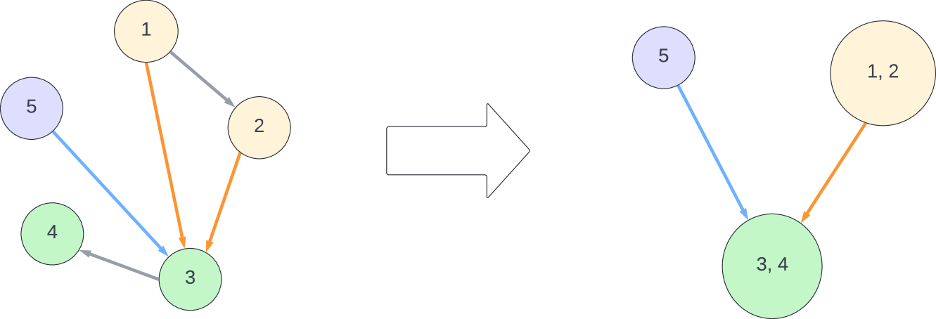
Given latent causal models parametrized by and as defined in Section 2.1, we say that there exists a structural causal model homomorphism between SCMs with parameters and if there exists a graph homomorphism , and measurable functions such that Eq(13) holds for all . See Fig. 2 for example.
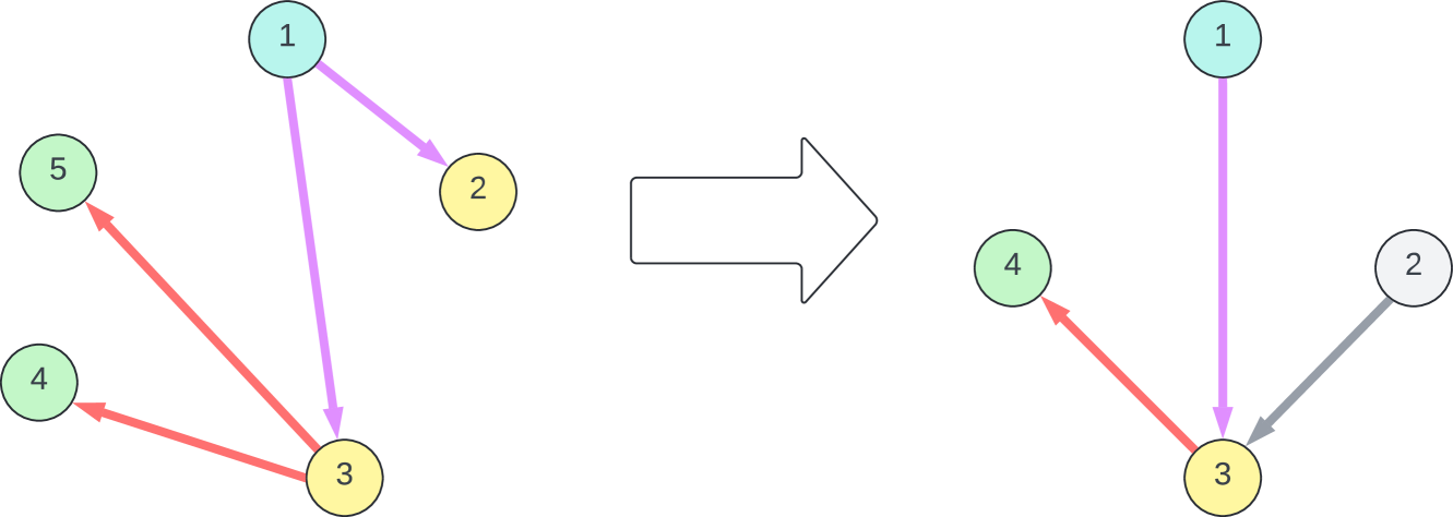
Definition 2.7 (SCM abstraction).
Given latent causal models parametrized by and as defined in Section 2.1, we say that
if there exists a SCM homomorphism between SCMs with parameters and , and the associated graph homomorphism is surjective (i.e. an epimorphism). See Fig. 3 for example.
Alternatively, we can say that is an abstraction of the SCM parameters .
Note that the above definition consists of a structural map in the form of a graph epimorphism, as well as a full set of distributional equivalences between all the latent components of two causal models that is compatible with the structural map, therefore it is easy to check that the following statement holds.
Lemma 2.4.
Given latent causal models parametrized by and as defined in Section 2.1, suppose . Then with respect to the canonical decompositions and .
Finally, we can check that the equivalence relations from Section 2.2 are consistent with the definitions of partial orders that give rise to the corresponding abstractions defined in this section.
Lemma 2.5.
Given latent causal models parametrized by and as defined in Section 2.1, and any
3 IDENTIFIABILITY RESULTS
3.1 PRELIMINARIES
Before presenting our main result, we will introduce several key concepts on which it is based, as well as some notation. We will assume that the reader is familiar with the definitions of -algebras and partitions, which can otherwise be found in Appendix A.
Family of non-descendants
Given a directed graph , the non-descendants of a subset of its vertices shall be denoted as , that is the intersection of the non-descendants of all the nodes in . Furthermore, for a family of intervention targets, we will denote the corresponding family of non-descendants as
-algebra generated by family of sets
Given a collection of subsets of a set , the -algebra generated by , denoted , is the smallest -algebra on that contains all the sets in . More formally, is the intersection of all -algebras on that contain , ensuring that satisfies the properties of a -algebra (containing the empty set, closed under complements and countable union).
Partition generated by -algebra
The partition generated by a -algebra on a set , denoted , is the collection of disjoint measurable sets in that together cover . More formally, it consists of the equivalence classes of the relation that considers two elements to be equivalent if every set in either contains both or contains neither. These equivalence classes form a partition, and each class is an element of the -algebra. This partition is maximal in the sense that the elements of the partition cannot be further subdivided using sets from .
Quotient graph generated by partition
The quotient graph of a directed graph with respect to a partition of the vertex set is defined such that the vertex set of is exactly , and for distinct blocks and in , there is a directed edge from to in if and only if there exists at least one directed edge from a vertex in to a vertex in in the original directed graph .
Graph condensations
Note that the definition above implies that given a directed acyclic graph and an arbitrary partition of its vertices, the resultant quotient graph can contain cycles. However, it is always true that there exists another quotient graph , known as the condensation of , that is acyclic. This is important because it ensures that we can always obtain an abstraction of some causal model for any partition of the vertices by taking the condensation.
We construct the condensation by taking the quotient of with respect to the partition defined by all the strongly connected components of , which are maximal subgraphs such that for all vertices , there exists a directed path from to and from to .
3.2 MAIN RESULTS
For both of the results stated in this section, we make the following assumptions on the hypothesis class of parameters
-
1.
Faithfulness of the causal graph: Let be a perfect map (Pearl, , 2009) for the distribution of , meaning that it encapsulates all the conditional independences.
-
2.
Absolute continuity of latent distributions: Let 444Here we use to denote isomorphic vector spaces, let , be continuously differentiable for all and , and let and be absolutely continuous.
-
3.
Smoothness of mixing function: Let be a diffeomorphism.
3.2.1 IDENTIFIABLE MODEL ABSTRACTION
Our first result shows that the parameters of a latent causal model as defined in Section 2.1 can be identified up to a SCM abstraction, depending on the non-descendant sets of the intervention targets.
Theorem 3.1.
Any latent causal model with parameters is identifiable up to a SCM abstraction with causal graph
| (14) |
meaning that for all
| (15) |
Furthermore, we can show that the quotient graph is acyclic, so we do not have to resort to taking its condensation.
Example 3.1.
Let be the latent causal model depicted in Fig. 1, so that . Then the corresponding family of non-descendants is , as shown by the subsets of blue vertices on the panel on the right of the figure. Hence we can compute the partition , and know that we can identify the latent causal model up to the SCM abstraction shown in Fig. 4.
3.2.2 ADDITIONAL IDENTIFIABLE LATENTS
Our second result follows from the first, and uses our definition of latent disentanglement to identify additional latents. Here we have a notion of equivalence between latent variables that correspond to the intersections of intervention targets with the same non-descendant sets, but no constraints on the causal mechanisms between them.
Theorem 3.2.
For any denote the intersection of all intervention targets with as their non-descendant set as
Now provided that is a singleton set and , then we can identify the latent up to disentanglement, meaning that for all
| (16) |
with respect to and some latent subspace in .
Example 3.2.
Let be the latent causal model depicted in Fig. 1, so that and as before. Then by looking at the intersections of subsets of blue vertices in each of the boxes with dotted lines, we can see that and . Thus we can disentangle the latent variable , provided that it takes value on .
3.3 PROOF OUTLINES
We leave the precise details of the proofs of Theorem 3.1 and Theorem 3.2 to Appendix C, and instead highlight some key properties of the data generating process that the proofs depend on. All together, these should serve as an outline of the main techniques used.
Finite mixtures
Since the intervention target is a discrete random variable and takes only a finite number of values, the latent distribution becomes a finite mixture of distributions with one mixture component for each value of
| (17) |
We will show that these components can be separated up to equivalence classes of where each component corresponds to an element .
| (18) |
Invariance of non-descendant variables
From Eq. 1 and Eq. 4, we can see that given any intervention target , the block of latents which correspond to the non-descendant set of (i.e. nodes in which are not descendants of any member of ), is invariant across the counterfactual pair, and crucially is the “maximally” invariant block. Formally, if we let denote the non-descendant set of then
| (19) | |||
| (20) |
Von Kügelgen et al., (2021) made use of this property to isolate the combined “content” block, , from the “style” block, which consists of the remainder of the latents, identifying the true causal model up to the abstraction . However, through a slightly more careful examination, we show that every block in can be disentangled (see Theorem 3.1). Essentially, this comes down to the fact that for each , the distribution is an absolutely continuous measure with non-zero mass on a submanifold of that uniquely identifies , since with respect to . Therefore we can obtain a matching of all latent blocks and their complements in the non-descendant sets of intervention targets, for any two latent causal models which produce the same observable distribution. Note that for this step, the assumption of absolute continuity of the latent distributions, together with the assumption of the smoothness of the mixing function are key.
Independence of interventional targets
From Eq. 3, we can see that given any intervention target , the block of post-intervention latents corresponding to is statistically independent of the pre-intervention latents. i.e. . Brehmer et al., (2022) made use of this property to disentangle for all , but under the restrictive assumption that consists precisely of all the atomic intervention targets 555an intervention target set is said to be atomic if for some node , so that no distinct intervention targets share the same non-descendant set. We remove this assumption, and instead disentangle (see Theorem 3.2) by making use of the fact that for all
| (21) |
Loosely, the equation above translates to the fact that with respect to the distribution of , which we managed to separate from the other mixture components of the total paired latent distribution as a result of the previous step, corresponds to the maximal partition of that is independent from . Note that the faithfulness of the causal graph is particularly important here, since we do not want to fail to take into account conditional independences which were not represented in the graph.
3.4 DISCUSSION
Theorem 3.1 implies that in order to identify the latent variables corresponding to a subset of nodes in the SCM up to abstraction, it is not necessary to have an intervention on directly (i.e. requiring ), which is perhaps surprising. Instead, it is sufficient to have .
Furthermore, this result implies that all distributional maps between “blocks” of variables are compatible with a structural map that abstracts to its quotient as defined in Eq. 14.
This is particularly relevant in cases of CRL problems where recovering the full causal graph is not possible due to lack of atomic interventions. In these scenarios, we can learn the causal structure up to an abstraction , meaning that while the causal relationships between certain latent variables corresponding to nodes in are not clear, the causal mechanisms between aggregated subsets of these variables corresponding to nodes in can be recovered correctly.
Additionally, Theorem 3.2 tells us that we can disentangle even more of the latent variables than the ones implied by Theorem 3.1, at the cost of disregarding the causal graph.
4 DOWNSTREAM APPLICATIONS AND LIMITATIONS
In terms of downstream tasks, our method has the usual applications for causal discovery, including causal effect estimation with respect to high-level variables; although we emphasize that in our particular problem formulation, none of the causal variables are directly observable, and therefore our work differs from the settings in classic ATE estimation or those presented in (Anand et al., , 2023).
Instead, we find that our weakly-supervised CRL setup makes assumptions that are more prevalent in recent machine learning literature, in which under unknown interventions counterfactual data pairs are indeed available, sometimes at the cost of the direct observability of causal variables. For example
-
•
In contrastive learning (Von Kügelgen et al., , 2021), pairs of data samples before and after random augmentations or transformations, which can be viewed as interventions, are used in order to learn latent representations with causal dependencies
-
•
In problems with temporal data (Lippe et al., , 2022), we may consider sequential observations of the system as our counterfactual data.
-
•
In the field of causal interpretability, specifically with respect to the method of interchange intervention training (Geiger et al., , 2022), we ay generate synthetic counterfactual data pairs by activation patching of neural networks.
In most machine learning applications, access to the latent causal structure can benefit generalization to out-of-distribution data. It can also serve as a foundation for interpretable and fair ML methods.
The eventual objective in CRL is having a methodology for learning the underlying latent causal model, up to some degree of abstraction. However, this is a distinct objective from having theoretical identifiability results, which demonstrate that should one succeed in learning an estimator of the model parameters which maximize the likelihood of observable distribution, then the true causal model is identified up to abstraction.
Learning remains an important problem of its own, and we make no claim in addressing that problem. Our example in Appendix D demonstrates a possible route for a small toy problem, and is by no mean a demonstration of a scalable method for identification of the abstract causal model, which we shall leave for future research.
5 CONCLUSION
We introduced a new framework for examining the identifiability of causal models up to abstraction. While previous works aiming to jointly learn the causal graph in conjunction with the latent variables have focused on fully identifying the graph up to isomorphism (Brehmer et al., , 2022; von Kügelgen et al., , 2024; Wendong et al., , 2024), we show that with relaxed assumptions, we can still recover a quotient graph and additional latent blocks that can all be determined from the family of intervention targets, which are not necessarily atomic and do not have to include all nodes of the graph. We argue that this is meaningful because in some ways, the identifiable causal model abstraction to constitutes the “real” ground truth model given the observable distribution, by the law of parsimony.
ACKNOWLEDGMENTS
This research was supported by CIFAR AI Chairs, NSERC Discovery, and Samsung AI Labs. Mila and Compute Canada provided computational resources. The authors would like to thank Sébastien Lachapelle for insightful discussions.
References
- Ahuja et al., (2022) Ahuja, K., Hartford, J. S., and Bengio, Y. (2022). Weakly supervised representation learning with sparse perturbations. Advances in Neural Information Processing Systems, 35:15516–15528.
- Ahuja et al., (2023) Ahuja, K., Mahajan, D., Wang, Y., and Bengio, Y. (2023). Interventional causal representation learning. In International conference on machine learning, pages 372–407. PMLR.
- Anand et al., (2023) Anand, T. V., Ribeiro, A. H., Tian, J., and Bareinboim, E. (2023). Causal effect identification in cluster dags. In Proceedings of the AAAI Conference on Artificial Intelligence, volume 37, pages 12172–12179.
- Beckers and Halpern, (2019) Beckers, S. and Halpern, J. Y. (2019). Abstracting causal models. In Proceedings of the aaai conference on artificial intelligence, volume 33, pages 2678–2685.
- Belyaeva et al., (2021) Belyaeva, A., Squires, C., and Uhler, C. (2021). Dci: learning causal differences between gene regulatory networks. Bioinformatics, 37(18):3067–3069.
- Bengio et al., (2013) Bengio, Y., Courville, A., and Vincent, P. (2013). Representation learning: A review and new perspectives. IEEE transactions on pattern analysis and machine intelligence, 35(8):1798–1828.
- Bloem-Reddy et al., (2020) Bloem-Reddy, B., Whye, Y., et al. (2020). Probabilistic symmetries and invariant neural networks. Journal of Machine Learning Research, 21(90):1–61.
- Brehmer et al., (2022) Brehmer, J., De Haan, P., Lippe, P., and Cohen, T. S. (2022). Weakly supervised causal representation learning. Advances in Neural Information Processing Systems, 35:38319–38331.
- Brouillard et al., (2020) Brouillard, P., Lachapelle, S., Lacoste, A., Lacoste-Julien, S., and Drouin, A. (2020). Differentiable causal discovery from interventional data. Advances in Neural Information Processing Systems, 33:21865–21877.
- Fong, (2013) Fong, B. (2013). Causal theories: A categorical perspective on bayesian networks. arXiv preprint arXiv:1301.6201.
- Geiger et al., (2024) Geiger, A., Ibeling, D., Zur, A., Chaudhary, M., Chauhan, S., Huang, J., Arora, A., Wu, Z., Goodman, N., Potts, C., et al. (2024). Causal abstraction: A theoretical foundation for mechanistic interpretability. Preprint.
- Geiger et al., (2021) Geiger, A., Lu, H., Icard, T., and Potts, C. (2021). Causal abstractions of neural networks. In Ranzato, M., Beygelzimer, A., Dauphin, Y., Liang, P., and Vaughan, J. W., editors, Advances in Neural Information Processing Systems, volume 34, pages 9574–9586. Curran Associates, Inc.
- Geiger et al., (2022) Geiger, A., Wu, Z., Lu, H., Rozner, J., Kreiss, E., Icard, T., Goodman, N., and Potts, C. (2022). Inducing causal structure for interpretable neural networks. In International Conference on Machine Learning, pages 7324–7338. PMLR.
- Gresele et al., (2020) Gresele, L., Rubenstein, P. K., Mehrjou, A., Locatello, F., and Schölkopf, B. (2020). The incomplete rosetta stone problem: Identifiability results for multi-view nonlinear ica. In Uncertainty in Artificial Intelligence, pages 217–227. PMLR.
- Hauser and Bühlmann, (2012) Hauser, A. and Bühlmann, P. (2012). Characterization and greedy learning of interventional markov equivalence classes of directed acyclic graphs. The Journal of Machine Learning Research, 13(1):2409–2464.
- Higgins et al., (2018) Higgins, I., Amos, D., Pfau, D., Racaniere, S., Matthey, L., Rezende, D., and Lerchner, A. (2018). Towards a definition of disentangled representations. arXiv preprint arXiv:1812.02230.
- Hyvärinen and Pajunen, (1999) Hyvärinen, A. and Pajunen, P. (1999). Nonlinear independent component analysis: Existence and uniqueness results. Neural networks, 12(3):429–439.
- Hyvarinen et al., (2019) Hyvarinen, A., Sasaki, H., and Turner, R. (2019). Nonlinear ica using auxiliary variables and generalized contrastive learning. In The 22nd International Conference on Artificial Intelligence and Statistics, pages 859–868. PMLR.
- Lippe et al., (2022) Lippe, P., Magliacane, S., Löwe, S., Asano, Y. M., Cohen, T., and Gavves, S. (2022). Citris: Causal identifiability from temporal intervened sequences. In International Conference on Machine Learning, pages 13557–13603. PMLR.
- Locatello et al., (2019) Locatello, F., Bauer, S., Lucic, M., Raetsch, G., Gelly, S., Schölkopf, B., and Bachem, O. (2019). Challenging common assumptions in the unsupervised learning of disentangled representations. In international conference on machine learning, pages 4114–4124. PMLR.
- Locatello et al., (2020) Locatello, F., Poole, B., Rätsch, G., Schölkopf, B., Bachem, O., and Tschannen, M. (2020). Weakly-supervised disentanglement without compromises. In International conference on machine learning, pages 6348–6359. PMLR.
- Massidda et al., (2023) Massidda, R., Geiger, A., Icard, T., and Bacciu, D. (2023). Causal abstraction with soft interventions. In Conference on Causal Learning and Reasoning, pages 68–87. PMLR.
- Otsuka and Saigo, (2022) Otsuka, J. and Saigo, H. (2022). On the equivalence of causal models: A category-theoretic approach. In Conference on Causal Learning and Reasoning, pages 634–646. PMLR.
- Pearl, (2009) Pearl, J. (2009). Causality. Cambridge university press.
- Rischel, (2020) Rischel, E. F. (2020). The category theory of causal models. Master’s thesis, University of Copenhagen.
- Rischel and Weichwald, (2021) Rischel, E. F. and Weichwald, S. (2021). Compositional abstraction error and a category of causal models. In Uncertainty in Artificial Intelligence, pages 1013–1023. PMLR.
- Rubenstein et al., (2017) Rubenstein, P. K., Weichwald, S., Bongers, S., Mooij, J. M., Janzing, D., Grosse-Wentrup, M., and Schölkopf, B. (2017). Causal consistency of structural equation models. arXiv preprint arXiv:1707.00819.
- Schölkopf et al., (2021) Schölkopf, B., Locatello, F., Bauer, S., Ke, N. R., Kalchbrenner, N., Goyal, A., and Bengio, Y. (2021). Toward causal representation learning. Proceedings of the IEEE, 109(5):612–634.
- Shu et al., (2019) Shu, R., Chen, Y., Kumar, A., Ermon, S., and Poole, B. (2019). Weakly supervised disentanglement with guarantees. arXiv preprint arXiv:1910.09772.
- Spirtes et al., (2001) Spirtes, P., Glymour, C., and Scheines, R. (2001). Causation, prediction, and search. MIT press.
- Verma and Pearl, (1990) Verma, T. and Pearl, J. (1990). Equivalence and synthesis of causal models. Probabilistic and Causal Inference.
- von Kügelgen et al., (2024) von Kügelgen, J., Besserve, M., Wendong, L., Gresele, L., Kekić, A., Bareinboim, E., Blei, D., and Schölkopf, B. (2024). Nonparametric identifiability of causal representations from unknown interventions. Advances in Neural Information Processing Systems, 36.
- Von Kügelgen et al., (2021) Von Kügelgen, J., Sharma, Y., Gresele, L., Brendel, W., Schölkopf, B., Besserve, M., and Locatello, F. (2021). Self-supervised learning with data augmentations provably isolates content from style. Advances in neural information processing systems, 34:16451–16467.
- Wendong et al., (2024) Wendong, L., Kekić, A., von Kügelgen, J., Buchholz, S., Besserve, M., Gresele, L., and Schölkopf, B. (2024). Causal component analysis. Advances in Neural Information Processing Systems, 36.
- Yang et al., (2018) Yang, K., Katcoff, A., and Uhler, C. (2018). Characterizing and learning equivalence classes of causal DAGs under interventions. In Dy, J. and Krause, A., editors, Proceedings of the 35th International Conference on Machine Learning, volume 80 of Proceedings of Machine Learning Research, pages 5541–5550. PMLR.
- Yao et al., (2023) Yao, D., Xu, D., Lachapelle, S., Magliacane, S., Taslakian, P., Martius, G., von Kügelgen, J., and Locatello, F. (2023). Multi-view causal representation learning with partial observability. arXiv preprint arXiv:2311.04056.
- Zennaro, (2022) Zennaro, F. M. (2022). Abstraction between structural causal models: A review of definitions and properties. arXiv preprint arXiv:2207.08603.
- Zhang et al., (2024) Zhang, J., Greenewald, K., Squires, C., Srivastava, A., Shanmugam, K., and Uhler, C. (2024). Identifiability guarantees for causal disentanglement from soft interventions. Advances in Neural Information Processing Systems, 36.
- Zimmermann et al., (2021) Zimmermann, R. S., Sharma, Y., Schneider, S., Bethge, M., and Brendel, W. (2021). Contrastive learning inverts the data generating process. In International Conference on Machine Learning, pages 12979–12990. PMLR.
CHECKLIST
-
1.
For all models and algorithms presented, check if you include:
-
(a)
A clear description of the mathematical setting, assumptions, algorithm, and/or model. [Yes]
-
(b)
An analysis of the properties and complexity (time, space, sample size) of any algorithm. [Not Applicable]
-
(c)
(Optional) Anonymized source code, with specification of all dependencies, including external libraries. [No]
-
(a)
-
2.
For any theoretical claim, check if you include:
-
(a)
Statements of the full set of assumptions of all theoretical results. [Yes]
-
(b)
Complete proofs of all theoretical results. [Yes]
-
(c)
Clear explanations of any assumptions. [Yes]
-
(a)
-
3.
For all figures and tables that present empirical results, check if you include:
-
(a)
The code, data, and instructions needed to reproduce the main experimental results (either in the supplemental material or as a URL). [Yes]
-
(b)
All the training details (e.g., data splits, hyperparameters, how they were chosen). [Yes]
-
(c)
A clear definition of the specific measure or statistics and error bars (e.g., with respect to the random seed after running experiments multiple times). [Not Applicable]
-
(d)
A description of the computing infrastructure used. (e.g., type of GPUs, internal cluster, or cloud provider). [Not Applicable]
-
(a)
-
4.
If you are using existing assets (e.g., code, data, models) or curating/releasing new assets, check if you include:
-
(a)
Citations of the creator If your work uses existing assets. [Not Applicable]
-
(b)
The license information of the assets, if applicable. [Not Applicable]
-
(c)
New assets either in the supplemental material or as a URL, if applicable. [Not Applicable]
-
(d)
Information about consent from data providers/curators. [Not Applicable]
-
(e)
Discussion of sensible content if applicable, e.g., personally identifiable information or offensive content. [Not Applicable]
-
(a)
-
5.
If you used crowdsourcing or conducted research with human subjects, check if you include:
-
(a)
The full text of instructions given to participants and screenshots. [Not Applicable]
-
(b)
Descriptions of potential participant risks, with links to Institutional Review Board (IRB) approvals if applicable. [Not Applicable]
-
(c)
The estimated hourly wage paid to participants and the total amount spent on participant compensation. [Not Applicable]
-
(a)
APPENDIX
Appendix A DEFINITIONS
Definition A.1 (-algebra).
A -algebra on a set is a collection of subsets of which satisfies the following properties
-
1.
Universality:
-
2.
Closure under Complements:
-
3.
Closure under Countable Union:
Definition A.2 (Partition).
A partition of a set is a collection of non-empty, pairwise disjoint subsets of such that:
-
1.
for all (the subsets are pairwise disjoint),
-
2.
(the union of all subsets covers ).
Definition A.3 (Group).
A group is a set equipped with a binary operation (often denoted by ) that satisfies the following four axioms:
-
1.
Closure: ,
-
2.
Associativity: ,
-
3.
Identity: such that ,
-
4.
Inverse: , such that
Definition A.4 (Group Action).
A group action of a group on a set is a map that satisfies the following two properties:
-
1.
Identity: For all , , where is the identity element of
-
2.
Compatibility: For all and , .
Definition A.5 (Stabilizer).
Let be a group acting on a set . For any element , the stabilizer of , denoted by , is the subgroup of consisting of all elements that fix
Definition A.6 (Diffeomorphism Group).
The diffeomorphism group on a differentiable manifold , denoted by , is the group of all smooth, invertible maps from to itself with smooth inverses. In other words, it consists of all bijective maps such that both and its inverse are differentiable. The group operation in is composition of maps. The identity element of is the identity map . The inverse of a diffeomorphism is its inverse map .
Definition A.7 (Pushforward Distributions).
The pushforward of a distribution describes how a probability distribution is transformed under a given function. Let be a measure space, where is a set, is a -algebra of measurable sets on , and is a measure for a distribution on . Let be a measurable function from to another measurable space . The pushforward of the measure under , denoted by , is a new measure on defined by:
In other words, the measure of a set under the pushforward measure is the measure of its preimage under the original measure .
Appendix B ASIDE ON DISTRIBUTIONAL ASYMMETRY
Given random variables and such that for some measurable function , we are motivated by the question: does the statistical independence of and imply the functional independence of and ? More formally, we want to know if the following holds
| (22) |
At first glance, the answer might seem to be yes. But suppose that has a standard Gaussian distribution on , has a uniform distribution over and , where denotes a clockwise rotation about the origin in . Then it is easy to see that the distribution is a 2D standard Gaussian for all , so , but certainly is not constant with respect to its second argument.
One way to guarantee that statistical independence implies function independence is by assuming that is smooth and that cannot be preserved by a “smoothly varying” family of diffeomorphisms, which we will show below.
Proposition B.1.
Suppose the stabilizer of the distribution is totally disconnected in the diffeomorphism group . Then the condition in Eq. 22 holds.
Proof.
First, note that the diffeomorphism group can act on the space of probability distributions on in a natural way. For any diffeomorphism and any probability distribution on , the pushforward of by , denoted by , is a new probability distribution on . We can thus easily check that the group action is well-defined.
Next, for any metric on we can equip with the following metric, where for we have . A set is said to be totally disconnected if there is no and such that . Intuitively, this means there is no smoothly varying family of diffeomorphisms in , however small.
Finally, consider the set of diffeomorphisms . By the smoothness of we can see that is connected in . Since the stabilizer of the distribution is totally disconnected in the diffeomorphism group , implies that
| (23) |
which means that is contained a left coset of the stabilzer of , and therefore must be totally disconnected. But since is connected this means that it is a singleton set, and hence there exists such that for all . ∎
Appendix C PROOFS
Theorem 3.1 Under the following assumptions on the hypothesis class of parameters , latent causal model with parameters is identifiable up to a causal model abstraction with directed acyclic causal graph
-
1.
Faithfulness of the causal graph: Let be a perfect map for the distribution of , meaning that it encapsulates all the conditional independences.
-
2.
Absolute continuity of latent distributions: Let , let , be continuously differentiable for all and , and let and be absolutely continuous.
-
3.
Smoothness of mixing function: Let be a diffeomorphism.
Proof.
Suppose we have such that . Denote the measures representing the distributions of and as and respectively. Denote their marginals and as and respectively. Let , and write . Then by definition of the data generating process
| (24) |
Finite Mixtures conditioned on Non-Descendants We can decompose these distributions into finite mixtures, so that we have
| (25) | ||||
| (26) |
where and denote the distributions and , and and denote the positive constants and .
Distributions of Latent Differences By a slight abuse of notation define the following operator on both and .
| (27) |
For any note that the support of is restricted to the subspace , and moreover is the maximal subset such that the support of can be restricted to the subspace .
So for distinct , is the maximal subset such that the union of the supports of and can be restricted to the subspace , and is the maximal subset such that the intersection of the supports of and can be restricted to the subspace .
Similarly, for distinct , is the maximal subset such that the union of the supports of and can be restricted to the subspace , and is the maximal subset such that the intersection of the supports of and can be restricted to the subspace .
Separating Non-Descendant Mixtures For all we can let be the maximal subset such that , so that this defines a bijection
| (28) |
such that for all
| (29) | |||
| (30) |
Disentangling Non-Descendant Sets The projection of onto consists only of components such that . So under , given , the joint distribution of the latent variables and is represented by a corresponding mixture of components where , so the support of each is restricted to . Therefore almost surely implies almost surely, meaning that is conditionally independent of given . Similarly, we can show that is conditionally independent of given . Hence there exists such that
| (31) |
Disentangling Complements of Non-Descendants The projection of onto only contains components if . Thus almost surely implies almost surely for all with , so almost surely. Therefore is conditionally independent of given . Similarly, we can show that is conditionally independent of given . Hence there exists such that
| (32) |
Disentangling Intersections If there are functions and identifying and then naturally their marginals would agree on such that they define a new function that identifies .
Identifying Quotient Graph Given that we have shown that we can identify all latents corresponding to complements of non-descendant sets as well as intersections, we can extend the such that for any we have and , and note that this is a bijection from to . Furthermore, using and to denote and respectively, we can now restrict to a bijection
| (33) |
This matching of partitions constitutes a graph isomorphism between the quotient graphs and , which is equivalent to a graph epimorphism from to . To show this, note that any edge in the quotient graph from a source block to a terminal block is the result of causal dependency between some vertices and , by faithfulness of the original graph. So since , we must have , which means . Therefore there is an edge from to in . The same of course holds for and .
Finally, we can quickly note that is indeed acyclic, since any cycle in implies that there exists a directed edge from the complement of a non-descendant set to itself, which violates the definition of a non-descendant set.
∎
Theorem C.1.
For any denote the intersection of all intervention targets with as their non-descendant set as
Now provided that is a singleton set and , then we can identify the latent up to disentanglement, meaning that for all
| (34) |
Proof.
To show that we can additionally identify , note that for any , by definition of the data generating process, there exists some deterministic function such that
| (35) |
Thus we can deduce
| (36) | ||||
| (37) | ||||
| (38) |
Note also that the latent distribution under satisfies . Therefore by Proposition B.1, there exists such that , since is a random variable with domain on , so the stabilizer of its distribution contains at most two elements – the identity and a reflection about a point on – and thus must be totally disconnectd.
∎
Appendix D EXPERIMENTS
SETUP
We generate synthetic data for linear Gaussian models, where the parameter space is defined as follows. For any directed acyclic graph with nodes, we let each of the nodes be equipped with the latent space . We let the distribution of the exogenous variables be a standard isotropic unit Gaussian and furthermore define , where the coefficients are sampled from a Gaussian mixture model that has two equal components with means ±1 and standard deviation 0.25. For the intervention parameters, we sample the new exogenous variables from unit Gaussians again and let be the identity for all subsets and . We then uniformly sample a rotation matrix with respect to the Haar measure for our mixing function .
RESULTS
We maximize the likelihood of a set of latent causal parameters over the parameter space for linear Gaussian models as described above via gradient descent, with respect to the observed data. We validate our theory by showing that for parameters with sufficiently high likelihood, the learned encoder inverts the ground truth mixing function up to the required level of abstraction, meaning that in particular, as a result of Theorem 3.1, is approximately a block diagonal matrix where each of the blocks corresponds to an element in .