The fast rate of convergence of the smooth adapted Wasserstein distance

Martin Larsson Carnegie Mellon University, Department of Mathematical Sciences, larsson@cmu.edu    Jonghwa Park Carnegie Mellon University, Department of Mathematical Sciences, jonghwap@andrew.cmu.edu    Johannes Wiesel Carnegie Mellon University & University of Copenhagen, Department of Mathematical Sciences, wiesel@cmu.edu
Abstract

Estimating a $d$-dimensional distribution $\mu$ by the empirical measure $\accentset{\smash{\raisebox{-3.25499pt}{\scalebox{0.8}{$\widehat{\phantom{x}}$}}}}{\mu}_{n}$ of its samples is an important task in probability theory, statistics and machine learning. It is well known that $\mathbb{E}[\mathcal{W}_{p}(\accentset{\smash{\raisebox{-3.25499pt}{\scalebox{0.8}{$\widehat{\phantom{x}}$}}}}{\mu}_{n},\mu)]\lesssim n^{-1/d}$ for $d>2p$, where $\mathcal{W}_{p}$ denotes the $p$-Wasserstein metric. An effective tool to combat this curse of dimensionality is the smooth Wasserstein distance $\mathcal{W}^{(\sigma)}_{p}$, which measures the distance between two probability measures after having convolved them with isotropic Gaussian noise $\mathcal{N}(0,\sigma^{2}\text{I})$. In this paper we apply this smoothing technique to the adapted Wasserstein distance. We show that the smooth adapted Wasserstein distance $\mathcal{A}\mathcal{W}_{p}^{(\sigma)}$ achieves the fast rate of convergence $\mathbb{E}[\mathcal{A}\mathcal{W}_{p}^{(\sigma)}(\accentset{\smash{\raisebox{-3.25499pt}{\scalebox{0.8}{$\widehat{\phantom{x}}$}}}}{\mu}_{n},\mu)]\lesssim n^{-1/2}$, if $\mu$ is subgaussian. This result follows from the surprising fact, that any subgaussian measure $\mu$ convolved with a Gaussian distribution has locally Lipschitz kernels.

Keywords: empirical measure, (smooth, adapted) Wasserstein distance, fast rate, curse of dimensionality, Lipschitz kernels

1 Introduction

Let the Borel probability measures $\mu$ and $\nu$ be the laws of two stochastic processes $X=(X_{t})_{t=1}^{T}$ and $Y=(Y_{t})_{t=1}^{T}$ on the path space $(\mathbb{R}^{d})^{T}$, where $d\geq 1$ and $T\geq 2$. Let furthermore $\mathcal{P}_{p}((\mathbb{R}^{d})^{T})$ denote the set of all Borel probability measures on $(\mathbb{R}^{d})^{T}$ with finite $p$-moments, where $1\leq p<\infty$ is fixed. The weak topology on $\mathcal{P}_{p}((\mathbb{R}^{d})^{T})$ is metrized by the $p$-Wasserstein distance

$\displaystyle\mathcal{W}_{p}(\mu,\nu):=\left(\inf_{\pi\in\operatorname{Cpl}(\mu,\nu)}\int\left|x-y\right|^{p}\pi(dx,dy)\right)^{1/p}.$ (1)

Here, $\left|\cdot\right|$ denotes the $\ell^{2}$-norm on $(\mathbb{R}^{d})^{T}$ and $\operatorname{Cpl}(\mu,\nu)$ is the set of all couplings of $\mu$ and $\nu$; see [35, 34, 33] for a general overview of optimal transport theory and the Wasserstein distance.

For computational as well as estimation purposes, $\mu$ is often approximated by its empirical distribution $\accentset{\smash{\raisebox{-3.25499pt}{\scalebox{0.8}{$\widehat{\phantom{x}}$}}}}{\mu}_{n}:=\frac{1}{n}\sum_{j=1}^{n}\delta_{X^{(j)}}$ where $X^{(1)},\ldots,X^{(n)}$ are i.i.d samples from $\mu$. By the Glivenko–Cantelli theorem, $\accentset{\smash{\raisebox{-3.25499pt}{\scalebox{0.8}{$\widehat{\phantom{x}}$}}}}{\mu}_{n}$ converges weakly to $\mu$ almost surely as the sample size $n$ approaches infinity. As a consequence, $\mathcal{W}_{p}(\accentset{\smash{\raisebox{-3.25499pt}{\scalebox{0.8}{$\widehat{\phantom{x}}$}}}}{\mu}_{n},\mu)$ vanishes with probability one. However, this convergence is severely impeded by an exponential dependence on the dimension $dT$ of the path space, posing a challenge for computational efficiency. In fact, [13] shows the sharp curse of dimensionality (COD) convergence rates $\mathbb{E}[\mathcal{W}_{p}(\accentset{\smash{\raisebox{-3.25499pt}{\scalebox{0.8}{$\widehat{\phantom{x}}$}}}}{\mu}_{n},\mu)]\leq Cn^{-1/(dT)}$ whenever $dT>2p$ and $\mu$ is supported on $([0,1]^{d})^{T}$.

In order to improve these convergence rates, the smooth $p$-Wasserstein distance $\mathcal{W}^{(\sigma)}_{p}$ was recently studied [16, 18, 17, 27, 32, 19, 20].

Definition 1 (Smooth Wasserstein distance).

Let $1\leq p<\infty$ and $\mu,\nu\in\mathcal{P}_{p}((\mathbb{R}^{d})^{T})$. The smooth $p$-Wasserstein distance between $\mu$ and $\nu$ with smoothing parameter $\sigma>0$ is defined as

$\displaystyle\mathcal{W}^{(\sigma)}_{p}(\mu,\nu):=\mathcal{W}_{p}(\mu\ast\mathcal{N}_{\sigma},\nu\ast\mathcal{N}_{\sigma}).$ (2)

Here $\ast$ denotes the convolution operator and $\mathcal{N}_{\sigma}=\mathcal{N}(0,\sigma^{2}\text{I}_{dT})$ is an isotropic Gaussian measure on $(\mathbb{R}^{d})^{T}$.

Smoothing $\mathcal{W}_{p}$ in this way leads to several interesting results. In particular, the expected $\mathcal{W}^{(\sigma)}_{p}$-distance between $\accentset{\smash{\raisebox{-3.25499pt}{\scalebox{0.8}{$\widehat{\phantom{x}}$}}}}{\mu}_{n}$ and $\mu$ exhibits dimension-free convergence rates; this clearly improves upon the classical Wasserstein convergence rates discussed above. The following list gives a general overview of known results for $\mathcal{W}^{(\sigma)}_{p}$:

  1. (1)

    The two metrics $\mathcal{W}^{(\sigma)}_{p}$ and $\mathcal{W}_{p}$ generate the same topology on $\mathcal{P}_{p}((\mathbb{R}^{d})^{T})$. See [16, 27].

  2. (2)

    In [18, 27] it is shown that $\mathbb{E}[\mathcal{W}^{(\sigma)}_{p}(\accentset{\smash{\raisebox{-3.25499pt}{\scalebox{0.8}{$\widehat{\phantom{x}}$}}}}{\mu}_{n},\mu)^{p}]\leq Cn^{-1/2}$ holds when $\mu$ has a finite $q$-moment for some $q>2(dT+p)$. This result implies the slow rate of convergence, i.e., $\mathbb{E}[\mathcal{W}^{(\sigma)}_{p}(\accentset{\smash{\raisebox{-3.25499pt}{\scalebox{0.8}{$\widehat{\phantom{x}}$}}}}{\mu}_{n},\mu)]\leq Cn^{-1/(2p)}$ for some $C>0$.

  3. (3)

    If $\int e^{\beta\left|x\right|^{2}}\mu(dx)<\infty$ for some $\beta>(p-1)/\sigma^{2}$ (requiring $\mu$ to be subgaussian), this can be improved to the fast rate of convergence, i.e., $\mathbb{E}[\mathcal{W}^{(\sigma)}_{p}(\accentset{\smash{\raisebox{-3.25499pt}{\scalebox{0.8}{$\widehat{\phantom{x}}$}}}}{\mu}_{n},\mu)]\leq Cn^{-1/2}$ for some $C>0$; see [27].

  4. (4)

    Under the same assumption as in (3), $\sqrt{n}\mathcal{W}^{(\sigma)}_{p}(\accentset{\smash{\raisebox{-3.25499pt}{\scalebox{0.8}{$\widehat{\phantom{x}}$}}}}{\mu}_{n},\mu)$ converges weakly to a supremum of a tight Gaussian process. Details can be found in [17, 32] for $p=1$ and [19, 20] for $p>1$.

When $p>1$, the fast rate implies strictly faster convergence than the slow rate. While establishing the slow rate (2) under minimal assumptions is of independent interest, the distributional limit (4) suggests that the fast rate (3) is sharp in general. As a simple example, take $\mu=\frac{1}{2}(\delta_{a}+\delta_{b})$ for $a\neq b$. Similar to [13, Example (a) on page 2], we have $\mathbb{E}[\mathcal{W}_{p}^{(\sigma)}(\accentset{\smash{\raisebox{-3.25499pt}{\scalebox{0.8}{$\widehat{\phantom{x}}$}}}}{\mu}_{n},\mu)]\geq Cn^{-1/2}$ (see Appendix A for details).

In this paper, we extend the smoothing technique for $\mathcal{W}_{p}^{(\sigma)}$ to the adapted Wasserstein distance $\mathcal{A}\mathcal{W}_{p}$ and study the statistical properties of its smoothed counterpart $\mathcal{A}\mathcal{W}_{p}^{(\sigma)}$, the smooth adapted Wasserstein distance. The adapted Wasserstein distance was introduced to address the following issue:

For many time-dependent operators $F:\mathcal{P}_{p}((\mathbb{R}^{d})^{T})\to\mathbb{R}$, $\liminf_{n\to\infty}|F(\mu_{n})-F(\mu)|>0$ even if $\lim_{n\to\infty}\mathcal{W}_{p}(\mu_{n},\mu)=0$.

Examples of such operators $F$ are the value functions of optimal stopping problems, the Doob decomposition, superhedging problems, utility maximization, stochastic programming and risk measurements [28, 29, 15, 2, 7]; these commonly account for the time-structure of $\mu$ and $\nu$. As we describe in more detail below, $\mathcal{A}\mathcal{W}_{p}$ generates the coarsest topology, which makes such operators continuous [8]. Having introduced $\mathcal{A}\mathcal{W}_{p}^{(\sigma)}$, the main result of this paper, presented in Theorem 4, can be summarized as follows:

If $\mu$ is subgaussian, then $\mathbb{E}[\mathcal{A}\mathcal{W}^{(\sigma)}_{p}(\mu,\accentset{\smash{\raisebox{-3.25499pt}{\scalebox{0.8}{$\widehat{\phantom{x}}$}}}}{\mu}_{n})]\lesssim 1/\sqrt{n}$, i.e., the fast rate of convergence holds for the smooth adapted Wasserstein distance.

Before discussing Theorem 4 in Section 1.4 in more detail, we first recall basic facts about $\mathcal{A}\mathcal{W}_{p}$ in Section 1.1 and review existing results on finite-sample guarantees for $\mathcal{A}\mathcal{W}_{p}$ in Section 1.2.

1.1 Adapted distances

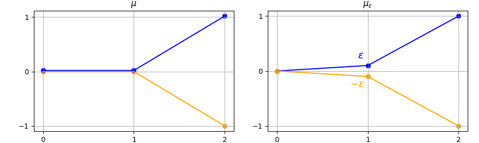
To illustrate the fact that the usual Wasserstein distance $\mathcal{W}_{p}$ is inadequate for time-dependent optimization problems, take $T=2,d=1$ and consider the laws $\mu=\frac{1}{2}\delta_{(0,1)}+\frac{1}{2}\delta_{(0,-1)}$ and $\mu_{\varepsilon}=\frac{1}{2}\delta_{(\varepsilon,1)}+\frac{1}{2}\delta_{(-\varepsilon,-1)}$. Figure 1 illustrates their sample paths. It is evident that $\mu_{\varepsilon}$ is close to $\mu$ in Wasserstein distance for small $\varepsilon$; in fact, $\mathcal{W}_{p}(\mu_{\varepsilon},\mu)=\varepsilon$. However, the process $X^{\varepsilon}\sim\mu^{\epsilon}$ differs significantly from $X\sim\mu$ as its values at time $2$ are already determined at time $1$. As a consequence, the values of utility maximization problems and optimal stopping problems for $\mu^{\epsilon}$ do not converge to the corresponding values for $\mu$.

Refer to caption
Figure 1: $\mu=\frac{1}{2}\delta_{(0,1)}+\frac{1}{2}\delta_{(0,-1)}$ on the left and $\mu_{\varepsilon}=\frac{1}{2}\delta_{(\varepsilon,1)}+\frac{1}{2}\delta_{(-\varepsilon,-1)}$ on the right.

To take the flow of information formalized through the natural filtration of a stochastic process into account, several variants of the weak topology have been independently developed by different communities, e.g., [24, 4, 22, 31, 21, 25, 1, 11]. Notably, [8] demonstrates that all these seemingly different variants of topologies coincide and are generated by the adapted Wasserstein distance. In order to define it formally, we first introduce the notion of bicausal couplings.

Definition 2 (Bicausal coupling).

Let $\mu$ and $\nu$ be two probability measures on $(\mathbb{R}^{d})^{T}$. A coupling $\pi\in\operatorname{Cpl}(\mu,\nu)$ is bicausal if for $(X,Y)\sim\pi$ and $t\in\{1,2,\ldots,T-1\}$,

$\displaystyle(Y_{1},\ldots,Y_{t})\text{ and }(X_{t+1},\ldots,X_{T})\text{ are conditionally independent given }X_{1},\ldots,X_{t},$ (3)

and

$\displaystyle(X_{1},\ldots,X_{t})\text{ and }(Y_{t+1},\ldots,Y_{T})\text{ are conditionally independent given }Y_{1},\ldots,Y_{t}.$ (4)

The set of all bicausal couplings between $\mu$ and $\nu$ is denoted by $\operatorname{Cpl_{bc}}(\mu,\nu)$.

Definition 3 (The adapted Wasserstein distance).

Let $1\leq p<\infty$ and $\mu,\nu\in\mathcal{P}_{p}((\mathbb{R}^{d})^{T})$. The adapted $p$-Wasserstein distance between $\mu$ and $\nu$ is defined as

$\displaystyle\mathcal{A}\mathcal{W}_{p}(\mu,\nu):=\left(\inf_{\pi\in\operatorname{Cpl_{bc}}(\mu,\nu)}\int\sum_{t=1}^{T}\left|x_{t}-y_{t}\right|^{p}\pi(dx,dy)\right)^{1/p}.$ (5)

Similarly to (2), the smooth adapted $p$-Wasserstein distance between $\mu$ and $\nu$ with smoothing parameter $\sigma>0$ is defined as

$\displaystyle\mathcal{A}\mathcal{W}^{(\sigma)}_{p}(\mu,\nu):=\mathcal{A}\mathcal{W}_{p}(\mu\ast\mathcal{N}_{\sigma},\nu\ast\mathcal{N}_{\sigma}).$ (6)

As mentioned above, the adapted Wasserstein distance induces the coarsest topology that makes optimal stopping problems continuous [8]. This topology is finer than the weak topology.

1.2 Approximations in adapted distances

Unlike the Wasserstein case, it is well-known (e.g., [30, 5]) that the empirical measure $\accentset{\smash{\raisebox{-3.25499pt}{\scalebox{0.8}{$\widehat{\phantom{x}}$}}}}{\mu}_{n}$ does not converge to $\mu$ in adapted Wasserstein distance as $n\to\infty$. To ensure approximation of $\mu$ by empirical data in adapted Wasserstein sense, [5] devise the so-called adapted empirical measure $\boldsymbol{\accentset{\smash{\raisebox{-3.25499pt}{\scalebox{0.8}{$\widehat{\phantom{x}}$}}}}{\mu}_{n}}$ as an alternative to the empirical measure $\accentset{\smash{\raisebox{-3.25499pt}{\scalebox{0.8}{$\widehat{\phantom{x}}$}}}}{\mu}_{n}$. It is defined as a projection of $\accentset{\smash{\raisebox{-3.25499pt}{\scalebox{0.8}{$\widehat{\phantom{x}}$}}}}{\mu}_{n}$ onto a refining grid and satisfies $\lim_{n\to\infty}\mathcal{A}\mathcal{W}_{p}(\boldsymbol{\accentset{\smash{\raisebox{-3.25499pt}{\scalebox{0.8}{$\widehat{\phantom{x}}$}}}}{\mu}_{n}},\mu)=0$. However the convergence rate obtained for $\boldsymbol{\accentset{\smash{\raisebox{-3.25499pt}{\scalebox{0.8}{$\widehat{\phantom{x}}$}}}}{\mu}_{n}}$ is essentially the same as the Wasserstein COD rates for $\mathbb{E}[\mathcal{W}_{p}(\accentset{\smash{\raisebox{-3.25499pt}{\scalebox{0.8}{$\widehat{\phantom{x}}$}}}}{\mu}_{n},\mu)]$. In fact, it was shown in [5, 3] that $\mathbb{E}[\mathcal{A}\mathcal{W}_{1}(\boldsymbol{\accentset{\smash{\raisebox{-3.25499pt}{\scalebox{0.8}{$\widehat{\phantom{x}}$}}}}{\mu}_{n}},\mu)]\leq Cn^{-1/(dT)}$ for some $C>0$ when $d\geq 3$ and $\mu$ is a probability measure on $([0,1]^{d})^{T}$ that has Lipschitz kernels. As $\mathcal{W}_{p}\leq C\mathcal{A}\mathcal{W}_{p}$ for some constant $C$ that depends only on $d,T$, the rates for $\mathbb{E}[\mathcal{A}\mathcal{W}_{1}(\boldsymbol{\accentset{\smash{\raisebox{-3.25499pt}{\scalebox{0.8}{$\widehat{\phantom{x}}$}}}}{\mu}_{n}},\mu)]$ are sharp.

Motivated by the non-adapted counterpart $\mathcal{W}^{(\sigma)}_{p}$, smoothing techniques have been introduced to achieve dimension-free adapted Wasserstein approximations. One of the earliest works in this direction is [30], which states that $\mathcal{A}\mathcal{W}_{p}(\mu,\accentset{\smash{\raisebox{-3.25499pt}{\scalebox{0.8}{$\widehat{\phantom{x}}$}}}}{\mu}_{n}\ast\eta_{\sigma_{n}})$ converges to zero in probability under arguably restrictive assumptions on $\mu$. Here $\eta_{\sigma_{n}}$ are non-Gaussian smoothing kernels converging weakly to the Dirac distribution $\delta_{0}$ for $\sigma_{n}\to 0$. Precise statements can be found in [30, Theorem $4$]. On the contrary, we keep $\sigma>0$ fixed throughout this work.

1.3 Prior results for the smooth adapted Wasserstein distance

Paralleling our list for $\mathcal{W}_{p}^{(\sigma)}$ above, let us now provide an overview of known results for $\mathcal{A}\mathcal{W}_{p}^{(\sigma)}$. It seems natural to conjecture that items (1)-(4) still hold when replacing $\mathcal{W}_{p}$ by $\mathcal{A}\mathcal{W}_{p}$ and $\mathcal{W}_{p}^{(\sigma)}$ by $\mathcal{A}\mathcal{W}_{p}^{(\sigma)}$. Perhaps surprisingly, it turns out that this is not the case, as already the first item on the list fails. Here is the corresponding list of facts for the adapted Wasserstein distance:

  1. (1)

    The two metrics $\mathcal{A}\mathcal{W}^{(\sigma)}_{p}$ and $\mathcal{W}_{p}$ generate the same topology on on $\mathcal{P}_{p}((\mathbb{R}^{d})^{T})$ [9]. Note that this is not the same topology as the one generated by $\mathcal{A}\mathcal{W}_{p}$.

  2. (2)

    For $p=1$, [23] shows that $\mathbb{E}[\mathcal{A}\mathcal{W}^{(\sigma)}_{1}(\accentset{\smash{\raisebox{-3.25499pt}{\scalebox{0.8}{$\widehat{\phantom{x}}$}}}}{\mu}_{n},\mu)]\leq Cn^{-1/2}$ for compactly supported $\mu$. For general $p\geq 1$, [9] shows that $\mathbb{E}[\mathcal{A}\mathcal{W}_{p}^{(\sigma)}(\accentset{\smash{\raisebox{-3.25499pt}{\scalebox{0.8}{$\widehat{\phantom{x}}$}}}}{\mu}_{n},\mu)^{p}]\leq Cn^{-1/2+p/(2q)}$ if $\int\left|x\right|^{q}\mu(dx)<\infty$ for some $q>p\vee(dT+2)$. In particular, if $\mu$ has a compact support, we can take $q$ arbitrarily large, resulting in the bound $\mathbb{E}[\mathcal{A}\mathcal{W}^{(\sigma)}_{p}(\accentset{\smash{\raisebox{-3.25499pt}{\scalebox{0.8}{$\widehat{\phantom{x}}$}}}}{\mu}_{n},\mu)^{p}]\leq Cn^{-1/2+\varepsilon}$ for arbitrarily small $\varepsilon>0$ and a constant $C>0$ depending on $\varepsilon$. This recovers the slow rate (2) for $\mathcal{A}\mathcal{W}^{(\sigma)}_{p}$, up to a loss of $\varepsilon$.

  3. (3)

    To the best of our knowledge, there is no existing result for the fast rate for $\mathcal{A}\mathcal{W}^{(\sigma)}_{p}$. Our paper fills this gap.

  4. (4)

    To the best of our knowledge, there is no result for the limiting distribution of $\sqrt{n}\mathcal{A}\mathcal{W}^{(\sigma)}_{p}(\accentset{\smash{\raisebox{-3.25499pt}{\scalebox{0.8}{$\widehat{\phantom{x}}$}}}}{\mu}_{n},\mu)$. We plan to address this question in future research.

Regarding the fast rate for $\mathcal{A}\mathcal{W}^{(\sigma)}_{p}$, the closest paper we could find is [10], where the authors introduce the so-called smoothed empirical martingale projection distance $\text{MPD}^{\ast\xi}(\accentset{\smash{\raisebox{-3.25499pt}{\scalebox{0.8}{$\widehat{\phantom{x}}$}}}}{\mu}_{n},p)$. It is defined as the minimal $\mathcal{A}\mathcal{W}^{p}_{p}$-value between $\accentset{\smash{\raisebox{-3.25499pt}{\scalebox{0.8}{$\widehat{\phantom{x}}$}}}}{\mu}_{n}\ast\xi$ for a smoothing distribution $\xi$ and the set of martingale measures (i.e., the set of measures $\nu$ satisfying $\mathbb{E}[X_{2}|X_{1}]=X_{1}$ if $(X_{1},X_{2})\sim\nu$). $\text{MPD}^{\ast\xi}(\accentset{\smash{\raisebox{-3.25499pt}{\scalebox{0.8}{$\widehat{\phantom{x}}$}}}}{\mu}_{n},p)$ is used to construct a test for the martingale property of $\mu$. When $\mu$ is a martingale measure, [10] shows that $n^{p/2}\text{MPD}^{\ast\xi}(\accentset{\smash{\raisebox{-3.25499pt}{\scalebox{0.8}{$\widehat{\phantom{x}}$}}}}{\mu}_{n},p)$ has a weak limit. Although $\xi$ is not necessarily Gaussian and their setting differs from ours, it reflects the spirit of the fast rate we aim to explore. This is why we will examine this example in more detail in Section 1.5.

1.4 Main results

We are now in a position to state our main result: the fast rate for the smooth adapted $p$-Wasserstein distance and subgaussian measures $\mu$.

Theorem 4 (Fast rate).

Let $1<p<\infty$ and $\sigma>0$. Suppose that $\mu$ is a probability measure on $(\mathbb{R}^{d})^{T}$, where $d\geq 1$ and $T\geq 2$, such that $\int e^{q\left|x\right|^{2}/(2\sigma^{2})}\mu(dx)<\infty$ for $q>8p(2p-1)(T+9)$. Then there exists a constant $C>0$ that depends only on $p,q,d,T,\sigma$ and $\int e^{q\left|x\right|^{2}/(2\sigma^{2})}\mu(dx)$ such that

$\displaystyle\mathbb{E}[\mathcal{A}\mathcal{W}^{(\sigma)}_{p}(\accentset{\smash{\raisebox{-3.25499pt}{\scalebox{0.8}{$\widehat{\phantom{x}}$}}}}{\mu}_{n},\mu)]\leq\frac{C}{\sqrt{n}}.$ (7)

Using the fact that $\mathcal{W}_{p}\leq C\mathcal{A}\mathcal{W}_{p}$ for some constant $C$ that depends only on $d,T$, Theorem 4 is sharp.

We detail the proof of Theorem 4 in Section 2. We also remark that the moment assumption $q>8p(2p-1)(T+9)$ can be relaxed. In fact, we will see in Section 2, that (7) holds if $q>\inf_{\beta}q^{*}(p,T,\beta)$, where the infimum is taken over all parameters $\beta$ in the set (P). We refer to (Q) for a precise definition of $q^{*}(p,T,\beta)$.

The proof of Theorem 4 combines the dynamic programming principle for the adapted Wasserstein distance (see Proposition 13) with the following rather surprising result, stating that any compactly supported measure convolved with Gaussian noise automatically has Lipschitz kernels:

Proposition 5 (Smoothed measures have Lipschitz kernels; exact statement in Proposition 6).

Suppose $\mu$ is a compactly supported probability measure on $(\mathbb{R}^{d})^{T}$. Then there exists a constant $C>0$ that depends only on $d,p,\sigma,\operatorname{supp}(\mu)$ such that

$\displaystyle\mathcal{W}_{p}((\mu\ast\mathcal{N}_{\sigma})_{x_{1:t}},(\mu\ast\mathcal{N}_{\sigma})_{y_{1:t}})\leq C\left|x_{1:t}-y_{1:t}\right|$ (8)

for all $x,y\in(\mathbb{R}^{d})^{T}$ and $t\in\{1,2,\ldots,T-1\}$. Here, $x_{1:t}$ denotes the first $t$ coordinates of $x$ and $(\mu\ast\mathcal{N}_{\sigma})_{x_{1:t}}$ is a probability measure on $\mathbb{R}^{d}$ defined via

$\displaystyle(\mu\ast\mathcal{N}_{\sigma})_{x_{1:t}}(dx_{t+1}):=\mathbb{P}(X_{t+1}\in dx_{t+1}\,|\,X_{1}=x_{1},\cdots,X_{t}=x_{t})$ (9)

for $X\sim\mu\ast\mathcal{N}_{\sigma}$.

In Proposition 6 below we extend this result to subgaussian measures, showing that a smoothed subgaussian measure has locally Lipschitz kernels. Since Lipschitz kernels naturally arise in many applications and are well-studied [5, 3, 9, 12], we believe that Proposition 6 is of independent interest.

1.5 Applications

We now present a concrete application of the fast rate (7), which is taken from [10]. Consider a probability measure $\mu$ on $(\mathbb{R}^{d})^{2}$. Recall that we call $\mu$ a martingale measure, if $\mathbb{E}[X_{2}|X_{1}]=X_{1}$ holds for $(X_{1},X_{2})\sim\mu$. Closely following [10], let us define the smoothed martingale projection distance (SMPD) via

$\displaystyle\text{SMPD}(\mu,p):=\inf\big{\{}\mathcal{A}\mathcal{W}_{p}(\mu\ast\xi,\nu)\,|\,\nu\text{ is a martingale measure}\big{\}}.$ (10)

Here we define $\xi$ as the law of $(Z_{1},Z_{1}+Z_{2})$, where $(Z_{1},Z_{2})$ are two independent Gaussian random variables with mean 0 and covariance matrix $\text{I}_{d}$. $\text{SMPD}(\mu,p)$ measures the $\mathcal{A}\mathcal{W}_{p}$-distance between $\mu\ast\xi$ and the space of martingale measures, and is used to test whether $\mu$ is a martingale measure. While [10] offers an in-depth analysis of this distance, let us emphasize here that $\mu$ is a martingale if and only if $\text{SMPD}(\mu,p)=0$. In particular, to test the martingale hypothesis using i.i.d samples, we aim to bound the probability

$\displaystyle\mathbb{P}\left(\left|\text{SMPD}(\mu,p)-\text{SMPD}(\accentset{\smash{\raisebox{-3.25499pt}{\scalebox{0.8}{$\widehat{\phantom{x}}$}}}}{\mu}_{n},p)\right|>\alpha\right)$ (11)

for $\alpha>0$. By the triangle inequality,

$\displaystyle\left|\text{SMPD}(\mu,p)-\text{SMPD}(\accentset{\smash{\raisebox{-3.25499pt}{\scalebox{0.8}{$\widehat{\phantom{x}}$}}}}{\mu}_{n},p)\right|\leq\mathcal{A}\mathcal{W}_{p}(\mu\ast\xi,\accentset{\smash{\raisebox{-3.25499pt}{\scalebox{0.8}{$\widehat{\phantom{x}}$}}}}{\mu}_{n}\ast\xi).$ (12)

Combined with the Markov inequality leads to

$\displaystyle\mathbb{P}\left(\left|\text{SMPD}(\mu,p)-\text{SMPD}(\accentset{\smash{\raisebox{-3.25499pt}{\scalebox{0.8}{$\widehat{\phantom{x}}$}}}}{\mu}_{n},p)\right|>\alpha\right)\leq\frac{\mathbb{E}[\mathcal{A}\mathcal{W}_{p}(\mu\ast\xi,\accentset{\smash{\raisebox{-3.25499pt}{\scalebox{0.8}{$\widehat{\phantom{x}}$}}}}{\mu}_{n}\ast\xi)]}{\alpha}.$ (13)

The fast rate (7) applied to the right hand side of (13) establishes the convergence rate $n^{-1/2}$, which is independent of the dimension $d$.

1.6 Notation and preparations

We close this section by setting up notation in Section 1.6. As mentioned above, $\left|\cdot\right|$ is the Euclidean norm, and we denote the scalar (dot) product by $\cdot$. Throughout the paper, $T\geq 2$ is the number of time steps and $d\geq 1$ is the dimension of the state space. The Hölder conjugate of $p$ is denoted by $p^{\prime}$, i.e., $1/p+1/p^{\prime}=1$.

For any Borel set $A$ in Euclidean space, the set of all Borel probability measures on $A$ is denoted by $\mathcal{P}(A)$. For $1\leq p<\infty$, $\mathcal{P}_{p}(A)$ is the set of all $\mu\in\mathcal{P}(A)$ that have finite $p$-moments, i.e., $\int\left|x\right|^{p}\mu(dx)<\infty$. For a measure $\mu$, we denote the pushforward measure of $\mu$ under a Borel function $T$ by $T_{\#}\mu$, i.e., $T_{\#}\mu(A)=\mu(\{x:T(x)\in A\})$ for all Borel sets $A$.

Given $X\sim\mu\in\mathcal{P}((\mathbb{R}^{d})^{T})$, we denote the mean of $X$ by $\operatorname{m}(\mu):=\int x\mu(dx)$. Also, the trace of the covariance matrix of $X$ is denoted by $\operatorname{var}(\mu):=\int\left|x-\operatorname{m}(\mu)\right|^{2}\mu(dx)$. For $r>0$, we define $M_{r}(\mu):=\int\left|x\right|^{r}\mu(dx)$ and $\mathcal{E}_{r}(\mu):=\int e^{r\left|x\right|^{2}}\mu(dx)$.

For $x\in(\mathbb{R}^{d})^{T}$ and $t\in\{1,2,\ldots,T\}$, we use the shorthand notation $x_{t}$ to denote the $t$-coordinate of $x$ and $x_{1:t}:=(x_{1},\ldots,x_{t})$. In particular, $x_{1:T}=x$. Similarly, given $\mu\in\mathcal{P}((\mathbb{R}^{d})^{T})$, we write $\mu_{t}$ for the projection of $\mu$ onto the $t$-coordinate and $\mu_{1:t}$ for the projection of $\mu$ onto the first $t$-coordinates. Precisely speaking, $\mu_{t}$=$P^{t}_{\#}\mu$ and $\mu_{1:t}=P^{1:t}_{\#}\mu$ for $P^{t}(x)=x_{t}$ and $P^{1:t}(x)=x_{1:t}$.

Given $x\in(\mathbb{R}^{d})^{T}$ and $\mu\in\mathcal{P}((\mathbb{R}^{d})^{T})$, recall that a disintegration(or kernel) of $\mu$ is a measure $\mu_{x_{1:t}}\in\mathcal{P}(\mathbb{R}^{d})$, $t\in\{1,2,\ldots,T\}$ which is defined via $\mu_{x_{1:t}}(dx_{t+1})=\mathbb{P}(X_{t+1}\in dx_{t+1}\;|\;X_{1:t}=x_{1:t})$ for $X\sim\mu\in\mathcal{P}((\mathbb{R}^{d})^{T})$.

Given $\sigma>0$, we write $\varphi_{\sigma}:(\mathbb{R}^{d})^{T}\to\mathbb{R}$ for the Gaussian density, i.e., $\varphi_{\sigma}(x)=(2\pi\sigma^{2})^{-dT/2}e^{-\left|x\right|^{2}/2}$. It is the density of the centered Gaussian measure on $(\mathbb{R}^{d})^{T}$ with covariance matrix $\sigma^{2}\text{I}_{dT}$, which is denoted by $\mathcal{N}_{\sigma}$. Given $\mu\in\mathcal{P}((\mathbb{R}^{d})^{T})$, $\mu\ast\mathcal{N}_{\sigma}$ is a convolution of $\mu$ and $\mathcal{N}_{\sigma}$, i.e., $\mu\ast\mathcal{N}_{\sigma}(A)=\int\mathcal{N}_{\sigma}(A-x)\mu(dx)$ for all measurable $A$. Note that $\mu\ast\mathcal{N}_{\sigma}$ has density $x\mapsto\varphi_{\sigma}\ast\mu(x)=\int\varphi_{\sigma}(x-y)\mu(dy)$. We use the shorthand notation $\mu^{\sigma}:=\mu\ast\mathcal{N}_{\sigma}$. For $t\in\{1,2,\ldots,T\}$, we abuse notation and write $\varphi_{\sigma}(x_{1:t})=(2\pi\sigma^{2})^{-dt/2}e^{-\left|x_{1:t}\right|^{2}/2}$. Similarly, $\mathcal{N}_{\sigma}$ can mean a centered Gaussian measure on $(\mathbb{R}^{d})^{t}$ with covariance matrix $\sigma^{2}\text{I}_{dt}$ depending on the context. Following the same reasoning, the density of $(P^{1:t}_{\#}\mu)^{\sigma}=(P^{1:t}_{\#}\mu)\ast\mathcal{N}_{\sigma}$ is denoted by $x_{1:t}\mapsto\varphi_{\sigma}\ast\mu(x_{1:t})=\int\varphi_{\sigma}(x_{1:t}-y_{1:t})\mu(dy_{1:t})$.

For a probability measure $\mu$ and i.i.d samples $X^{(1)},X^{(2)},\ldots,X^{(n)}$ of $\mu$, we define the empirical measure of $\mu$ via $\accentset{\smash{\raisebox{-3.25499pt}{\scalebox{0.8}{$\widehat{\phantom{x}}$}}}}{\mu}_{n}=\frac{1}{n}\sum_{j=1}^{n}\delta_{X^{(j)}}$. Note that this is a measure-valued random variable. Adopting the same notation as above, we write $\accentset{\smash{\raisebox{-3.25499pt}{\scalebox{0.8}{$\widehat{\phantom{x}}$}}}}{\mu}^{\sigma}_{n}$ for $\accentset{\smash{\raisebox{-3.25499pt}{\scalebox{0.8}{$\widehat{\phantom{x}}$}}}}{\mu}_{n}\ast\mathcal{N}_{\sigma}$.

Let $\mu\in\mathcal{P}(A)$ for some Borel set $A$ in a Euclidean space. For $1\leq p<\infty$, $L^{p}(\mu;\mathbb{R}^{k})$ is the set of all functions $f:A\to\mathbb{R}^{k}$ such that $\left\|f\right\|_{L^{p}(\mu;\mathbb{R}^{k})}:=(\int_{A}\left|f\right|^{p}d\mu)^{1/p}<\infty$. When $k=1$, we often write $L^{p}(\mu)\>=L^{p}(\mu;\mathbb{R}^{k})$. We denote by $C_{c}^{\infty}(\mathbb{R}^{N})$ the set of all smooth functions $h:\mathbb{R}^{N}\to\mathbb{R}$ with compact support. For the multi-index $\alpha=(\alpha_{1},\ldots,\alpha_{N})$ and $h\in\mathbb{R}^{N}\to\mathbb{R}$, we write $\left|\alpha\right|=\sum_{j=1}^{N}\alpha_{j}$ and denote the $\alpha$-th derivative of $h$ by $\partial^{\alpha}h(x)=\frac{\partial^{\alpha_{1}}}{\partial x_{1}^{\alpha_{1}}}\frac{\partial^{\alpha_{2}}}{\partial x_{2}^{\alpha_{2}}}\cdots\frac{\partial^{\alpha_{N}}}{\partial x_{N}^{\alpha_{N}}}h(x)$.

If $\gamma$ is a finite signed measure on $\mathbb{R}^{N}$ and $\mathcal{F}$ is a class of functions on $\mathbb{R}^{N}$, we identify $\gamma$ with the linear functional $g\mapsto\gamma(g):=\int gd\gamma$ on $\mathcal{F}$ and denote its $\ell^{\infty}(\mathcal{F})$-norm by $\left\|\gamma\right\|_{\mathcal{F}}:=\sup\{\gamma(g):g\in\mathcal{F}\}$.

2 Proof of Theorem 4

Unless otherwise stated, the parameters $1<p<\infty$ and $\sigma>0$ are fixed throughout the remainder of this note. Furthermore we always assume that $T\geq 2$ and $d\geq 1$.

The proof of Theorem 4 is divided into three parts: Section 2.1, Section 2.2 and Section 2.3. In Section 2.1 we prove Proposition 6, which states that the smoothed measures have locally Lipschitz kernels. In Section 2.2 we combine Propostion 6 with the dynamic programming principle for $\mathcal{A}\mathcal{W}_{p}$ stated in Proposition 13 and establish an upper bound for the $\mathcal{A}\mathcal{W}^{(\sigma)}_{p}$-distance between $\mu$ and $\accentset{\smash{\raisebox{-3.25499pt}{\scalebox{0.8}{$\widehat{\phantom{x}}$}}}}{\mu}_{n}$. Using empirical process theory (see Lemma 18), we prove Theorem 4 in Section 2.3.

2.1 Kernels of smoothed measures

This section is mainly devoted to the proof of Proposition 6. As mentioned in Section 1, a subgaussian measure convolved with Gaussian noise has locally Lipschitz kernels. Moreover, if the measure is compactly supported, then its kernels are Lipschitz.

Proposition 6 (Kernels of a smoothed measure).

Let $0<\beta<1/p^{\prime}$. Suppose that $\mu\in\mathcal{P}((\mathbb{R}^{d})^{T})$ satisfies $\mathcal{E}_{q/(2\sigma^{2})}(\mu)<\infty$ for $q>2(p-1)/\beta$. Then there exists a constant $C>0$ that depends only on $d,p,\sigma,q,\beta,\mathcal{E}_{q/(2\sigma^{2})}(\mu)$ such that for all $x,y\in(\mathbb{R}^{d})^{T}$ and $t\in\{1,2,\ldots,T-1\}$,

$\displaystyle\mathcal{W}_{p}((\mu^{\sigma})_{x_{1:t}},(\mu^{\sigma})_{y_{1:t}})\leq Ce^{\frac{\beta}{\sigma^{2}}\left(\left|x_{1:t}-\operatorname{m}(\mu_{1:t})\right|\vee\left|y_{1:t}-\operatorname{m}(\mu_{1:t})\right|\right)^{2}}\left|x_{1:t}-y_{1:t}\right|.$ (14)

In particular, if $\mu$ is compactly supported,

$\displaystyle\mathcal{W}_{p}((\mu^{\sigma})_{x_{1:t}},(\mu^{\sigma})_{y_{1:t}})\leq C\left|x_{1:t}-y_{1:t}\right|$ (15)

for some constant $C>0$ that depends only on $d,p,\sigma,\operatorname{supp}(\mu)$.

The proof is based on [19, Proposition $2.1$] which shows that the Wasserstein distance $\mathcal{W}_{p}$ can be bounded above by the dual Sobolev norm.

Proposition 7 (Proposition $2.1$ in [19]).

Let $1\leq p<\infty$ and suppose that $\mu_{0},\mu_{1}\in\mathcal{P}(\mathbb{R}^{d})$ with $\mu_{0},\mu_{1}\ll\rho$ for some reference measure $\rho\in\mathcal{P}(\mathbb{R}^{d})$. Denote their respective densities by $f_{i}=d\mu_{i}/d\rho$, $i=0,1$. If $f_{0}$ or $f_{1}$ is bounded from below by some $c>0$, then

$\displaystyle\mathcal{W}_{p}(\mu_{0},\mu_{1})\leq pc^{-1/p^{\prime}}\sup\left\{(\mu_{1}-\mu_{0})(\psi):\psi\in C^{\infty}_{c}(\mathbb{R}^{d}),\left\|\nabla\psi\right\|_{L^{p^{\prime}}(\rho;\mathbb{R}^{d})}\leq 1\right\}.$ (16)
Remark 8.

When $p=1$, a density argument applied to the Kantorovich–Rubinstein duality for $\mathcal{W}_{1}(\mu_{0},\mu_{1})$ shows that equality holds in (16). Note that the supremum in (16) is the operator norm of $(\mu_{1}-\mu_{0})$ in the dual of the homogeneous Sobolev space $\dot{H}^{1,p^{\prime}}$. See [27, 19] for details.

We will apply Proposition 7 to kernels of smoothed measures. To proceed, we define a function class $\mathcal{F}^{\sigma,p}$ for $1<p<\infty$, which is essentially the function class appearing in (16) adapted to our setting:

$\displaystyle\mathcal{F}^{\sigma,p}:=\{\psi-\mathcal{N}_{\sigma\eta}(\psi):\psi\in C^{\infty}_{c}(\mathbb{R}^{d}),\left\|\nabla\psi\right\|_{L^{p^{\prime}}(\mathcal{N}_{\sigma\eta};\mathbb{R}^{d})}\leq 1\}\text{ where }\eta:=\sqrt{1/(2p)^{\prime}}=\sqrt{1-\frac{1}{2p}}.$ (17)

The reason for the choice $\rho=\mathcal{N}_{\sigma\eta}$ will become apparent below.

Lemma 9.

Let $\mu\in\mathcal{P}_{2}((\mathbb{R}^{d})^{T})$, $x\in(\mathbb{R}^{d})^{T}$ and $t\in\{1,2,\ldots,T\}$.

  1. (a)

    If $0<a_{1}<a_{2}$, then

    $\displaystyle(\varphi^{a_{2}}_{\sigma}\ast\mu(x_{1:t}))^{1/a_{2}}\leq e^{\frac{(1-a_{1}/a_{2})}{2\sigma^{2}}\operatorname{var}(\mu_{1:t})}e^{\frac{(1-a_{1}/a_{2})}{2\sigma^{2}}\left|x_{1:t}-\operatorname{m}(\mu_{1:t})\right|^{2}}(\varphi^{a_{1}}_{\sigma}\ast\mu(x_{1:t}))^{1/a_{1}}.$ (18)
  2. (b)

    If $0<a<1$ and $h\in L^{1/a}(\mu)$, then

    $\displaystyle\int\varphi_{\sigma}(x_{1:t}-y_{1:t})\left|h(y_{1:T})\right|\mu(dy)\leq\left\|h\right\|_{L^{1/a}(\mu)}e^{\frac{a}{2\sigma^{2}}\operatorname{var}(\mu_{1:t})}e^{\frac{a}{2\sigma^{2}}\left|x_{1:t}-\operatorname{m}(\mu_{1:t})\right|^{2}}\varphi_{\sigma}\ast\mu(x_{1:t}).$ (19)
Proof.

(a): From Jensen’s inequality and

$$\int\left|x_{1:t}-y_{1:t}\right|^{2}\mu(dy)=|x_{1:t}-\operatorname{m}(\mu_{1:t})|^{2}+\operatorname{var}(\mu_{1:t})$$

we obtain

$\displaystyle\varphi^{a_{1}}_{\sigma}\ast\mu(x_{1:t})$ $\displaystyle=\int(2\pi\sigma^{2})^{-a_{1}dt/2}e^{-\frac{a_{1}\left|x_{1:t}-y_{1:t}\right|^{2}}{2\sigma^{2}}}\mu(dy)$ (20)
$\displaystyle\geq(2\pi\sigma^{2})^{-a_{1}dt/2}e^{-\frac{a_{1}\int\left|x_{1:t}-y_{1:t}\right|^{2}\mu(dy)}{2\sigma^{2}}}=(2\pi\sigma^{2})^{-a_{1}dt/2}e^{-\frac{a_{1}}{2\sigma^{2}}\operatorname{var}(\mu_{1:t})}e^{-\frac{a_{1}}{2\sigma^{2}}\left|x_{1:t}-\operatorname{m}(\mu_{1:t})\right|^{2}}.$ (21)

Thus, we obtain

$\displaystyle(\varphi^{a_{1}}_{\sigma}\ast\mu(x_{1:t}))^{1/a_{1}}$ $\displaystyle=(\varphi^{a_{1}}_{\sigma}\ast\mu(x_{1:t}))^{1/a_{2}}(\varphi^{a_{1}}_{\sigma}\ast\mu(x_{1:t}))^{1/a_{1}-1/a_{2}}$ (22)
$\displaystyle\geq(\varphi^{a_{1}}_{\sigma}\ast\mu(x_{1:t}))^{1/a_{2}}\left((2\pi\sigma^{2})^{-a_{1}dt/2}e^{-\frac{a_{1}}{2\sigma^{2}}\operatorname{var}(\mu_{1:t})}e^{-\frac{a_{1}}{2\sigma^{2}}\left|x_{1:t}-\operatorname{m}(\mu_{1:t})\right|^{2}}\right)^{1/a_{1}-1/a_{2}}$ (23)
$\displaystyle=[(2\pi\sigma^{2})^{-dt(a_{2}-a_{1})/2}\varphi^{a_{1}}_{\sigma}\ast\mu(x_{1:t})]^{1/a_{2}}e^{-\frac{(1-a_{1}/a_{2})}{2\sigma^{2}}\operatorname{var}(\mu_{1:t})}e^{-\frac{(1-a_{1}/a_{2})}{2\sigma^{2}}\left|x_{1:t}-\operatorname{m}(\mu_{1:t})\right|^{2}}.$ (24)

Since $(2\pi\sigma^{2})^{dt/2}\varphi_{\sigma}\leq 1$ on $(\mathbb{R}^{d})^{t}$ by definition and $a_{2}>a_{1}$, we have

$\displaystyle[(2\pi\sigma^{2})^{-dt(a_{2}-a_{1})/2}\varphi^{a_{1}}_{\sigma}\ast\mu(x_{1:t})]^{1/a_{2}}$ $\displaystyle=[(2\pi\sigma^{2})^{dt/2}\varphi_{\sigma})]^{a_{1}-a_{2}}\varphi_{\sigma}^{a_{2}}\ast\mu(x_{1:t}))^{1/a_{2}}$ (25)
$\displaystyle\geq(\varphi^{a_{2}}_{\sigma}\ast\mu(x_{1:t}))^{1/a_{2}}.$ (26)

This shows the desired result.

(b): Set $r:=1/a>1$ and use Hölder’s inequality to see that

$\displaystyle\int\varphi_{\sigma}(x_{1:t}-y_{1:t})\left|h(y_{1:T})\right|\mu(dy_{1:T})\leq\left\|h\right\|_{L^{r}(\mu)}(\varphi^{r^{\prime}}_{\sigma}\ast\mu(x_{1:t}))^{1/r^{\prime}}.$ (27)

Applying the previous part (a) with $a_{1}=1$ and $a_{2}=r^{\prime}>1$ we obtain

$\displaystyle(\varphi^{r^{\prime}}_{\sigma}\ast\mu(x_{1:t}))^{1/r^{\prime}}\leq e^{\frac{a}{2\sigma^{2}}\operatorname{var}(\mu_{1:t})}e^{\frac{a}{2\sigma^{2}}\left|x_{1:t}-\operatorname{m}(\mu_{1:t})\right|^{2}}\varphi_{\sigma}\ast\mu(x_{1:t}).$ (28)

This ends the proof. $\Box$

Lemma 10.

Let $0<\beta<1/p^{\prime}$. Suppose that $\mu\in\mathcal{P}((\mathbb{R}^{d})^{T})$ satisfies $\mathcal{E}_{q_{0}/(2\sigma^{2})}(\mu)<\infty$, where $q_{0}=2(p-1)(1/\beta-p^{\prime})>0$. If $\gamma\in\mathcal{P}((\mathbb{R}^{d})^{T})$ is absolutely continuous with respect to the Lebesgue measure, then for all $x\in(\mathbb{R}^{d})^{T}$ and $t\in\{1,2,\ldots,T-1\}$,

$\displaystyle\mathcal{W}_{p}((\mu^{\sigma})_{x_{1:t}},\gamma)\leq Ce^{\frac{\beta}{2\sigma^{2}}\left|x_{1:t}-\operatorname{m}\left(\mu_{1:t}\right)\right|^{2}}\left\|(\mu^{\sigma})_{x_{1:t}}-\gamma\right\|_{\mathcal{F}^{\sigma,p}},$ (29)

where $C=p((2p)^{\prime})^{d/(2p^{\prime})}(\mathcal{E}_{q_{0}/(2\sigma^{2})}(\mu_{t+1}))^{\beta/(1-\beta p^{\prime})}e^{\frac{\beta}{2\sigma^{2}}\operatorname{var}\left(\mu_{1:t}\right)}$.

Proof.

Recall $\eta=\sqrt{1/(2p)^{\prime}}$ as defined in (17). The proof follows from applying Proposition 7 to the reference measure $\rho:=\mathcal{N}_{\sigma\eta}$, once we have shown the following lower bound for the density:

$\displaystyle\frac{d(\mu^{\sigma})_{x_{1:t}}}{d\mathcal{N}_{\sigma\eta}}(x_{t+1})$ $\displaystyle=\frac{\varphi_{\sigma}\ast\mu(x_{1:t+1})}{\varphi_{\sigma}\ast\mu(x_{1:t})\varphi_{\sigma\eta}(x_{t+1})}$ (30)
$\displaystyle\geq\eta^{d}e^{-\frac{\beta p^{\prime}}{2\sigma^{2}}\operatorname{var}(\mu_{1:t})}(\mathcal{E}_{q_{0}/(2\sigma^{2})}(\mu_{t+1}))^{-\beta p^{\prime}/(1-\beta p^{\prime})}e^{-\frac{\beta p^{\prime}}{2\sigma^{2}}\left|x_{1:t}-\operatorname{m}(\mu_{1:t})\right|^{2}}.$ (31)

The well-known inequality $|x_{t+1}-y_{t+1}|^{2}\leq|x_{t+1}|^{2}/\eta^{2}+|y_{t+1}|^{2}/(1-\eta^{2})$ implies

$\displaystyle\varphi_{\sigma}(x_{t+1}-y_{t+1})=(2\pi\sigma^{2})^{-d/2}e^{-\frac{\left|x_{t+1}-y_{t+1}\right|^{2}}{2\sigma^{2}}}\geq\eta^{d}\varphi_{\sigma\eta}(x_{t+1})e^{-\frac{\left|y_{t+1}\right|^{2}}{2\sigma^{2}(1-\eta^{2})}}.$ (32)

We thus conclude that

$\displaystyle\varphi_{\sigma}\ast\mu(x_{1:t+1})$ $\displaystyle=\int\varphi_{\sigma}(x_{1:t}-y_{1:t})\varphi_{\sigma}(x_{t+1}-y_{t+1})\mu(dy)$
$\displaystyle\geq\eta^{d}\varphi_{\sigma\eta}(x_{t+1})\int\varphi_{\sigma}(x_{1:t}-y_{1:t})e^{-\frac{\left|y_{t+1}\right|^{2}}{2\sigma^{2}(1-\eta^{2})}}\mu(dy).$

We now apply the reverse Hölder inequality

$\displaystyle\int fgd\mu\geq\left(\int f^{1/r}d\mu\right)^{r}\left(\int g^{-1/(r-1)}d\mu\right)^{-(r-1)}$ (33)

with $r=\frac{1}{1-\beta p^{\prime}}>1$, $f(y_{1:t})=\varphi_{\sigma}(x_{1:t}-y_{1:t})$ and $g(y_{t+1})=e^{-\frac{\left|y_{t+1}\right|^{2}}{2\sigma^{2}(1-\eta^{2})}}$. Noting that

$\displaystyle\frac{1}{r}=1-\beta p^{\prime},\quad\frac{1}{1-\eta^{2}}\frac{1}{r-1}=2p\frac{1-\beta p^{\prime}}{\beta p^{\prime}}=q_{0},$ (34)

this gives

$\displaystyle\eta^{d}\varphi_{\sigma\eta}(x_{t+1})\int\varphi_{\sigma}(x_{1:t}-y_{1:t})e^{-\frac{\left|y_{t+1}\right|^{2}}{2\sigma^{2}(1-\eta^{2})}}\mu(dy)$ (35)
$\displaystyle\geq\eta^{d}\varphi_{\sigma\eta}(x_{t+1})(\varphi^{1-\beta p^{\prime}}_{\sigma}\ast\mu(x_{1:t}))^{\frac{1}{1-\beta p^{\prime}}}(\mathcal{E}_{q_{0}/(2\sigma^{2})}(\mu_{t+1}))^{-\beta p^{\prime}/(1-\beta p^{\prime})}.$ (36)

Choosing $a_{1}=1-\beta p^{\prime}<1=a_{2}$ in Lemma 9.(a) and noting that $(1-a_{1}/a_{2})=\beta p^{\prime}$, we obtain

$\displaystyle(\varphi^{1-\beta p^{\prime}}_{\sigma}\ast\mu(x_{1:t}))^{\frac{1}{1-\beta p^{\prime}}}\geq\varphi_{\sigma}\ast\mu(x_{1:t})e^{-\frac{\beta p^{\prime}}{2\sigma^{2}}\left|x_{1:t}-\operatorname{m}(\mu_{1:t})\right|^{2}}e^{-\frac{\beta p^{\prime}}{2\sigma^{2}}\operatorname{var}(\mu_{1:t})}.$ (37)

Combining (36) and (37) yields the desired result. $\Box$

Let us recall that the Gaussian measure $\mathcal{N}_{\sigma}$ on $\mathbb{R}^{d}$ satisfies the $r$-Poincare inequality [26, Theorem 2.4] for all $1\leq r<\infty$: there exists a constant $D>0$ that depends only on $d,r,\sigma$ such that

$\displaystyle\left\|\psi-\mathcal{N}_{\sigma}(\psi)\right\|_{L^{r}(\mathcal{N}_{\sigma})}\leq D\left\|\nabla\psi\right\|_{L^{r}(\mathcal{N}_{\sigma};\mathbb{R}^{d})}\text{ for all }\psi\in C^{\infty}_{c}(\mathbb{R}^{d}).$ (38)

In particular, for $f\in\mathcal{F}^{\sigma,p}$ and $\eta=\sqrt{1/(2p)^{\prime}}$, there exists a constant $D_{p,d,\sigma}>0$ that depends only on $p,d,\sigma$ such that

$\displaystyle\left\|f\right\|_{L^{p^{\prime}}(\mathcal{N}_{\sigma\eta})}\leq D_{p,d,\sigma}.$ (39)

For ease of reference we record the following computation.

Lemma 11.

Let $f\in\mathcal{F}^{\sigma,p}$ and recall the constant $D_{p,d,\sigma}$ in (39).

  1. (a)

    If $x\in\mathbb{R}^{d}$, then

    $\displaystyle\left|f\right|\ast\varphi_{\sigma}(x)\leq D_{p,d,\sigma}(2^{1/p}/(2p)^{\prime})^{d/2}e^{\frac{(p-1)\left|x\right|^{2}}{\sigma^{2}}}.$ (40)
  2. (b)

    If $\mu\in\mathcal{P}((\mathbb{R}^{d})^{T})$, $x,y\in(\mathbb{R}^{d})^{T}$ and $t\in\{1,2,\ldots,T-1\}$,

    $\displaystyle\int\left|f(x_{t+1})\right|\varphi_{\sigma}\ast\mu(x_{1:t+1})dx_{t+1}\leq D_{p,d,\sigma}(2^{1/p}/(2p)^{\prime})^{d/2}\int\varphi_{\sigma}(x_{1:t}-y_{1:t})e^{\frac{(p-1)\left|y_{t+1}\right|^{2}}{\sigma^{2}}}\mu(dy).$ (41)
Proof.

(a): We first apply Hölder’s inequality and (39) to obtain

$\displaystyle\left|f\right|\ast\varphi_{\sigma}(x)=\int\left|f(y)\right|\varphi_{\sigma\eta}^{-1}(y)\varphi_{\sigma}(x-y)\mathcal{N}_{\sigma\eta}(dy)$ $\displaystyle\leq\left\|f\right\|_{L^{p^{\prime}}(\mathcal{N}_{\sigma\eta};\mathbb{R}^{d})}\left(\int\varphi^{1-p}_{\sigma\eta}(y)\varphi^{p}_{\sigma}(x-y)dy\right)^{1/p}$ (42)
$\displaystyle\leq D_{p,d,\sigma}\left(\int\varphi^{1-p}_{\sigma\eta}(y)\varphi^{p}_{\sigma}(x-y)dy\right)^{1/p}.$ (43)

To conclude the proof of (a), it suffices to show that

$\displaystyle\int\varphi_{\sigma\eta}^{1-p}(y)\varphi^{p}_{\sigma}(x-y)dy=2^{d/2}(1-1/(2p))^{dp/2}e^{\frac{p(p-1)\left|x\right|^{2}}{\sigma^{2}}}.$ (44)

To see this, let us first note that for any $0<a<b$,

$\displaystyle\int_{\mathbb{R}^{d}}e^{a\left|y\right|^{2}-b\left|x-y\right|^{2}}dy=e^{\frac{ab}{b-a}\left|x\right|^{2}}\int_{\mathbb{R}^{d}}e^{-(b-a)\left|y-\frac{b}{b-a}x\right|^{2}}dy=(\pi/(b-a))^{d/2}e^{\frac{ab}{b-a}\left|x\right|^{2}}.$ (45)

Here, the first equality follows from $a\left|y\right|^{2}-b\left|x-y\right|^{2}=-(b-a)|y-\frac{b}{b-a}x|^{2}+\frac{ab}{b-a}\left|x\right|^{2}$. If we choose $a:=(p-1)/(2\sigma^{2}\eta^{2})$ and $b:=p/(2\sigma^{2})$, we have $b>a$ as

$\displaystyle\frac{p-1}{\eta^{2}}=\frac{p-1}{2p-1}2p<p.$ (46)

Furthermore,

$\displaystyle\varphi^{1-p}_{\sigma\eta}(y)\varphi^{p}_{\sigma}(x-y)=(2\pi\sigma^{2}\eta^{2})^{d(p-1)/2}(2\pi\sigma^{2})^{-dp/2}e^{a\left|y\right|^{2}-b\left|x-y\right|^{2}}.$ (47)

Thus, by (45),

$\displaystyle\int\varphi_{\sigma\eta}^{1-p}(y)\varphi^{p}_{\sigma}(x-y)dy=(2\pi\sigma^{2}\eta^{2})^{d(p-1)/2}(2\pi\sigma^{2})^{-dp/2}(\pi/(b-a))^{d/2}e^{\frac{ab}{b-a}\left|x\right|^{2}}.$ (48)

This shows the desired result noting that

$\displaystyle b-a=\frac{p}{2\sigma^{2}}-\frac{p-1}{2\sigma^{2}\eta^{2}}=\frac{p}{2\sigma^{2}}\Big{(}1-\frac{2p-2}{2p-1}\Big{)}=\frac{p}{2\sigma^{2}}\frac{1}{2p-1}=\frac{1}{4\sigma^{2}\eta^{2}},$

and

$\displaystyle\frac{ab}{b-a}=\frac{(p-1)p}{(2\sigma^{2})^{2}\eta^{2}}4\sigma^{2}\eta^{2}=\frac{(p-1)p}{\sigma^{2}}.$ (49)

(b): By Fubini’s theorem,

$\displaystyle\int\left|f(x_{t+1})\right|\varphi_{\sigma}\ast\mu(x_{1:t+1})dx_{t+1}$ $\displaystyle=\int\int\left|f(x_{t+1})\right|\varphi_{\sigma}(x_{1:t+1}-y_{1:t+1})\mu(dy_{1:t+1})dx_{t+1}$ (50)
$\displaystyle=\int\varphi_{\sigma}(x_{1:t}-y_{1:t})\left|f\right|\ast\varphi_{\sigma}(y_{t+1})\mu(dy).$ (51)

We now apply the previous result (a) to bound $\left|f\right|\ast\varphi_{\sigma}(y_{t+1})$. This concludes the proof. $\Box$

A Taylor expansion combined with Lemma 11 shows the following lemma.

Lemma 12.

Let $0<\beta<1$. Suppose that $\mu\in\mathcal{P}((\mathbb{R}^{d})^{T})$ satisfies $\mathcal{E}_{q/(2\sigma^{2})}(\mu)<\infty$, where $q>2(p-1)/\beta$. Then for all $x,y\in(\mathbb{R}^{d})^{T}$ and $t\in\{1,2,\ldots,T-1\}$,

$\displaystyle\left\|(\mu^{\sigma})_{x_{1:t}}-(\mu^{\sigma})_{y_{1:t}}\right\|_{\mathcal{F}^{\sigma,p}}\leq Ce^{\frac{\beta}{2\sigma^{2}}\left(\left|x_{1:t}-\operatorname{m}(\mu_{1:t})\right|\vee\left|y_{1:t}-\operatorname{m}(\mu_{1:t})\right|\right)^{2}}\left|x_{1:t}-y_{1:t}\right|,$ (52)

where

$\displaystyle C=\sigma^{-2}D_{p,d,\sigma}(2^{1/p}/(2p)^{\prime})^{d/2}e^{\frac{\beta}{2\sigma^{2}}\operatorname{var}(\mu_{1:t})}\left(\left\|h\right\|_{L^{1/\beta}(\mu)}+(M_{r}(\mu_{1:t}))^{1/r}(\mathcal{E}_{q/(2\sigma^{2})}(\mu_{1:t}))^{2(p-1)/q}\right)$ (53)

with $D_{p,d,\sigma}$ defined in (39), $h(w)=\left|w_{1:t}\right|e^{\frac{(p-1)\left|w_{t+1}\right|^{2}}{\sigma^{2}}}$ and $r=\frac{q}{\beta q-2(p-1)}$.

Proof.

For $f\in\mathcal{F}^{\sigma,p}$, note that

$\displaystyle((\mu^{\sigma})_{x_{1:t}}-(\mu^{\sigma})_{y_{1:t}})(f)=\int f(z_{t+1})\left(\frac{\varphi_{\sigma}\ast\mu(x_{1:t},z_{t+1})}{\varphi_{\sigma}\ast\mu(x_{1:t})}-\frac{\varphi_{\sigma}\ast\mu(y_{1:t},z_{t+1})}{\varphi_{\sigma}\ast\mu(y_{1:t})}\right)dz_{t+1}.$ (54)

Let $x_{1:t}(s):=sx_{1:t}+(1-s)y_{1:t}$ for $s\in[0,1]$ and set $g(s):=\frac{\varphi_{\sigma}\ast\mu(x_{1:t}(s),z_{t+1})}{\varphi_{\sigma}\ast\mu(x_{1:t}(s))}$. From Fubini’s theorem and $g(1)-g(0)=\int_{0}^{1}g^{\prime}(s)ds$ we have

$\displaystyle((\mu^{\sigma})_{x_{1:t}}-(\mu^{\sigma})_{y_{1:t}})(f)\leq\int_{0}^{1}\left(\int\left|f(z_{t+1})\right|\left|g^{\prime}(s)\right|dz_{t+1}\right)ds.$ (55)

Let us define $\kappa\in\mathcal{P}((\mathbb{R}^{d})^{T})$ via $\kappa(A):=\frac{1}{\varphi_{\sigma}\ast\mu(x_{1:t}(s))}\int_{A}\varphi_{\sigma}(x_{1:t}(s)-w_{1:t})\mu(dw_{1:t})$. We compute

$\displaystyle\frac{d}{ds}\log(\varphi_{\sigma}\ast\mu(x_{1:t}(s),z_{t+1}))$ (56)
$\displaystyle=-\frac{1}{\varphi_{\sigma}\ast\mu(x_{1:t}(s),z_{t+1})}\int\varphi_{\sigma}(x_{1:t}(s)-w_{1:t},z_{t+1}-w_{t+1})\Big{(}\frac{x_{1:t}(s)-w_{1:t}}{\sigma^{2}}\Big{)}\cdot\left(x_{1:t}-y_{1:t}\right)\mu(dw)$ (57)
$\displaystyle=-\frac{x_{1:t}(s)\cdot(x_{1:t}-y_{1:t})}{\sigma^{2}}+\frac{1}{\sigma^{2}g(s)}\int\varphi_{\sigma}(z_{t+1}-w_{t+1})w_{1:t}\cdot(x_{1:t}-y_{1:t})\kappa(dw).$ (58)

Similarly,

$\displaystyle\frac{d}{ds}\log(\varphi_{\sigma}\ast\mu(x_{1:t}(s)))=-\frac{x_{1:t}(s)\cdot(x_{1:t}-y_{1:t})}{\sigma^{2}}+\frac{1}{\sigma^{2}}\int w_{1:t}\cdot(x_{1:t}-y_{1:t})\kappa(dw).$ (59)

Canceling terms

$\displaystyle\frac{g^{\prime}(s)}{g(s)}=\frac{d}{ds}\log(g(s))=\frac{1}{\sigma^{2}g(s)}\int\varphi_{\sigma}(z_{t+1}-w_{t+1})w_{1:t}\cdot(x_{1:t}-y_{1:t})\kappa(dw)-\frac{1}{\sigma^{2}}\int w_{1:t}\cdot(x_{1:t}-y_{1:t})\kappa(dw).$ (60)

Hence we bound

$\displaystyle\left|g^{\prime}(s)\right|\leq\frac{\left|x_{1:t}-y_{1:t}\right|}{\sigma^{2}}\left(\int\varphi_{\sigma}(z_{t+1}-w_{t+1})\left|w_{1:t}\right|\kappa(dw)+g(s)\int\left|w_{1:t}\right|\kappa(dw_{1:t})\right).$ (61)

By applying this bound along with Fubini’s theorem, we obtain

$\displaystyle\int\left|f(z_{t+1})\right|\left|g^{\prime}(s)\right|dz_{t+1}$ (62)
$\displaystyle\leq\frac{\left|x_{1:t}-y_{1:t}\right|}{\sigma^{2}}\left(\int\left|f\right|\ast\varphi_{\sigma}(w_{t+1})\left|w_{1:t}\right|\kappa(dw)+\int\left|f(z_{t+1})\right|g(s)dz_{t+1}\int\left|w_{1:t}\right|\kappa(dw)\right)$ (63)
$\displaystyle=:\frac{\left|x_{1:t}-y_{1:t}\right|}{\sigma^{2}}(\text{I}+\text{II}).$ (64)

It remains to bound $\text{I}+\text{II}$. For this, using Lemma 11(a) and Lemma 9(b) for $x_{1:t}(s)$ instead of $x_{1:t}$,

I $\displaystyle\leq D_{p,d,\sigma}(2^{1/p}/(2p)^{\prime})^{d/2}\int\left|w_{1:t}\right|e^{\frac{(p-1)\left|w_{t+1}\right|^{2}}{\sigma^{2}}}\kappa(dw)$ (65)
$\displaystyle\leq D_{p,d,\sigma}(2^{1/p}/(2p)^{\prime})^{d/2}\left\|h\right\|_{L^{1/\beta}(\mu)}e^{\frac{\beta}{2\sigma^{2}}\operatorname{var}(\mu_{1:t})}e^{\frac{\beta}{2\sigma^{2}}\left|x_{1:t}(s)-\operatorname{m}(\mu_{1:t})\right|^{2}},$ (66)

where $h(w):=\left|w_{1:t}\right|e^{\frac{(p-1)\left|w_{t+1}\right|^{2}}{\sigma^{2}}}$. Similarly, we can establish

$\displaystyle\text{II}\leq D_{p,d,\sigma}(2^{1/p}/(2p)^{\prime})^{d/2}\left((M_{r}(\mu_{1:t}))^{1/r}(\mathcal{E}_{q/(2\sigma^{2})}(\mu_{t+1}))^{2(p-1)/q}\right)$ (67)
$\displaystyle\hskip 142.26378pt\cdot e^{\frac{\beta}{2\sigma^{2}}\operatorname{var}(\mu_{1:t})}e^{\frac{\beta}{2\sigma^{2}}\left|x_{1:t}(s)-\operatorname{m}(\mu_{1:t})\right|^{2}},$ (68)

where $r:=\frac{q}{\beta q-2(p-1)}>1$. Indeed, Lemma 11(b) shows

II $\displaystyle=\frac{1}{\varphi_{\sigma}\ast\mu(x_{1:t}(s))}\int\left|f(z_{t+1})\right|\varphi_{\sigma}\ast\mu(x_{1:t}(s),z_{t+1})dz_{t+1}\int\left|w_{1:t}\right|\kappa(dw)$ (69)
$\displaystyle\leq D_{p,d,\sigma}(2^{1/p}/(2p)^{\prime})^{d/2}\int e^{\frac{(p-1)\left|w_{t+1}\right|^{2}}{\sigma^{2}}}\kappa(dw)\int\left|w_{1:t}\right|\kappa(dw).$ (70)

To see (68), we apply Lemma 9(b) to $a=\beta-2(p-1)/q=1/r\in(0,1)$ for $x_{1:t}(s)$, which yields

$\displaystyle\int\left|w_{1:t}\right|\kappa(dw)\leq(M_{r}(\mu_{1:t}))^{1/r}e^{\frac{\beta-2(p-1)/q}{2\sigma^{2}}\operatorname{var}(\mu_{1:t})}e^{\frac{\beta-2(p-1)/q}{2\sigma^{2}}\left|x_{1:t}(s)-\operatorname{m}(\mu_{1:t})\right|^{2}}.$ (71)

By choosing $a=2(p-1)/q\in(0,1)$ in Lemma 9(b),

$\displaystyle\int e^{\frac{(p-1)\left|w_{t+1}\right|^{2}}{\sigma^{2}}}\kappa(dw)\leq(\mathcal{E}_{q/(2\sigma^{2})}(\mu_{t+1}))^{2(p-1)/q}e^{\frac{2(p-1)/q}{2\sigma^{2}}\operatorname{var}(\mu_{1:t})}e^{\frac{2(p-1)/q}{2\sigma^{2}}\left|x_{1:t}(s)-\operatorname{m}(\mu_{1:t})\right|^{2}}.$ (72)

This shows (68). By plugging (66) and (68) into (55) and using $|x_{1:t}(s)-\operatorname{m}(\mu_{1:t})|\leq|x_{1:t}-\operatorname{m}(\mu_{1:t})|\vee|y_{1:t}-\operatorname{m}(\mu_{1:t})|$, this concludes the proof of the lemma. $\Box$

Proof of Proposition 6.

It is easy to check that the moment assumptions of Lemma 10 and Lemma 12 are satisfied. We denote the constant apppering in Lemma 10 by $C_{1}$, and the constant appearing in Lemma 12 by $C_{2}$. Then from Lemma 10 and Lemma 12,

$\displaystyle\mathcal{W}_{p}((\mu^{\sigma})_{x_{1:t}},(\mu^{\sigma})_{y_{1:t}})$ $\displaystyle\leq C_{1}e^{\frac{\beta}{2\sigma^{2}}\left|x_{1:t}-\operatorname{m}(\mu_{1:t})\right|^{2}}\left\|(\mu^{\sigma})_{x_{1:t}}-(\mu^{\sigma})_{y_{1:t}}\right\|_{\mathcal{F}^{\sigma,p}}$ (73)
$\displaystyle\leq C_{1}C_{2}e^{\frac{\beta}{2\sigma^{2}}\left|x_{1:t}-\operatorname{m}(\mu_{1:t})\right|^{2}}e^{\frac{\beta}{2\sigma^{2}}\left(\left|x_{1:t}-\operatorname{m}(\mu_{1:t})\right|\vee\left|y_{1:t}-\operatorname{m}(\mu_{1:t})\right|\right)^{2}}\left|x_{1:t}-y_{1:t}\right|.$ (74)

Since the moments of $\mu$ appearing in $C_{1}$ and $C_{2}$ can be all bounded from above by $\mathcal{E}_{q/(2\sigma^{2})}(\mu)$, this proves the general case. When $\mu$ is compactly supported, we can get the desired result by sending $\beta\to 0$. Indeed, by translating the support of $\mu$ if necessary, we may assume that $0\in\operatorname{supp}(\mu)$. Next we note that the constant $C_{1}$ in Lemma 10 has a finite limit as $\beta\to 0$. Indeed, as $\beta\to 0$,

$\displaystyle C_{1}=p((2p)^{\prime})^{d/(2p^{\prime})}\left(\mathcal{E}_{\frac{p-1}{\sigma^{2}}(\frac{1}{\beta}-p^{\prime})}(\mu_{t+1})\right)^{\beta/(1-\beta p^{\prime})}e^{\frac{\beta}{2\sigma^{2}}\operatorname{var}(\mu_{1:t})}\longrightarrow p((2p)^{\prime})^{d/(2p^{\prime})}\left\|g\right\|^{(p-1)/\sigma^{2}}_{L^{\infty}(\mu_{t+1})},$ (75)

where $g(x_{t+1}):=e^{\left|x_{t+1}\right|^{2}}$. In particular, we bound

$\displaystyle\lim_{\beta\to 0}C_{1}\leq p((2p)^{\prime})^{d/(2p^{\prime})}e^{\frac{(p-1)\operatorname{diam}(\operatorname{supp}(\mu_{t+1}))}{\sigma^{2}}}.$ (76)

Similarly, the constant $C_{2}$ has a finite limit as $\beta\to 0$ and this limit can be controlled using $p,d,\sigma,\operatorname{supp}(\mu)$. This proves Proposition 6. $\Box$

2.2 Dynamic programming principle

In this section, we prove Lemma 15, which states that $\mathcal{A}\mathcal{W}^{(\sigma)}_{p}(\mu,\accentset{\smash{\raisebox{-3.25499pt}{\scalebox{0.8}{$\widehat{\phantom{x}}$}}}}{\mu}_{n})$ can be bounded above by a sum of $\mathcal{W}_{2p}$-distances between the kernels of $\mu^{\sigma}$ and $\accentset{\smash{\raisebox{-3.25499pt}{\scalebox{0.8}{$\widehat{\phantom{x}}$}}}}{\mu}^{\sigma}_{n}$ under suitable moment assumptions on $\mu$. To achieve this, we first apply Proposition 6 to $\mathcal{W}_{2p}$ and then incorporate it into the dynamic programming principle (DPP) for the adapted Wasserstein distance [6, Proposition $5.1$] which we present next.

Proposition 13 (Proposition $5.1$ in [6]).

Given $\mu,\nu\in\mathcal{P}_{p}((\mathbb{R}^{d})^{T})$, let us define $V_{t}:(\mathbb{R}^{d})^{t}\times(\mathbb{R}^{d})^{t}\to\mathbb{R}$, $t\in\{1,2,\ldots,T\}$ and $V_{0}\in\mathbb{R}$ via the following recursive formula: $V_{T}=0$ and for $t\in\{0,1,\ldots,T-1\}$,

$\displaystyle V_{t}(x_{1:t},y_{1:t})=\inf_{\gamma_{x_{1:t},y_{1:t}}\in\operatorname{Cpl}(\mu_{x_{1:t}},\nu_{y_{1:t}})}\int\left|x_{t+1}-y_{t+1}\right|^{p}+V_{t+1}(x_{1:t+1},y_{1:t+1})\gamma_{x_{1:t},y_{1:t}}(dx_{t+1},dy_{t+1}),$ (77)

where $\mu_{x_{1:0}}:=\mu_{1}$ and $\nu_{y_{1:0}}:=\nu_{1}$. Then $V_{0}=\mathcal{A}\mathcal{W}_{p}(\mu,\nu)^{p}$.

The following example illustrates how the DPP together with Proposition 6 is used to establish an upper bound for $\mathcal{A}\mathcal{W}^{(\sigma)}_{p}(\mu,\accentset{\smash{\raisebox{-3.25499pt}{\scalebox{0.8}{$\widehat{\phantom{x}}$}}}}{\mu}_{n})$ when $\mu$ is compactly supported.

Example 14 (Compact case).

If $\mu$ has a compact support, then there exists a constant $C>0$ that depends only on $d,T,p,\sigma,\operatorname{supp}(\mu)$ such that

$\displaystyle\mathcal{A}\mathcal{W}^{(\sigma)}_{p}(\mu,\accentset{\smash{\raisebox{-3.25499pt}{\scalebox{0.8}{$\widehat{\phantom{x}}$}}}}{\mu}_{n})\leq C\left(\mathcal{W}^{(\sigma)}_{p}(\mu_{1},(\accentset{\smash{\raisebox{-3.25499pt}{\scalebox{0.8}{$\widehat{\phantom{x}}$}}}}{\mu}_{n})_{1})+\sum_{t=1}^{T-1}\left(\int\mathcal{W}_{p}((\mu^{\sigma})_{y_{1:t}},(\accentset{\smash{\raisebox{-3.25499pt}{\scalebox{0.8}{$\widehat{\phantom{x}}$}}}}{\mu}^{\sigma}_{n})_{y_{1:t}})^{p}\accentset{\smash{\raisebox{-3.25499pt}{\scalebox{0.8}{$\widehat{\phantom{x}}$}}}}{\mu}^{\sigma}_{n}(dy)\right)^{1/p}\right)\text{ a.s. }$ (78)
Proof.

We follow the proof of [5, Lemma $3.1$] closely. Suppose $T=2$. Then Proposition 13 shows that

$\displaystyle\mathcal{A}\mathcal{W}^{(\sigma)}_{p}(\mu,\accentset{\smash{\raisebox{-3.25499pt}{\scalebox{0.8}{$\widehat{\phantom{x}}$}}}}{\mu}_{n})^{p}=\inf_{\gamma\in\operatorname{Cpl}((\mu^{\sigma})_{1},(\accentset{\smash{\raisebox{-3.25499pt}{\scalebox{0.8}{$\widehat{\phantom{x}}$}}}}{\mu}^{\sigma}_{n})_{1})}\int\left|x_{1}-y_{1}\right|^{p}+\mathcal{W}_{p}((\mu^{\sigma})_{x_{1}},(\accentset{\smash{\raisebox{-3.25499pt}{\scalebox{0.8}{$\widehat{\phantom{x}}$}}}}{\mu}^{\sigma}_{n})_{y_{1}})^{p}\gamma(dx_{1},dy_{1})$ (79)

From Proposition 6, $\mu^{\sigma}$ has Lipschitz kernels. Using this fact with the triangle inequality, we find

$\displaystyle\mathcal{W}_{p}((\mu^{\sigma})_{x_{1}},(\accentset{\smash{\raisebox{-3.25499pt}{\scalebox{0.8}{$\widehat{\phantom{x}}$}}}}{\mu}^{\sigma}_{n})_{y_{1}})^{p}$ $\displaystyle\leq C\mathcal{W}_{p}((\mu^{\sigma})_{x_{1}},(\mu^{\sigma})_{y_{1}})^{p}+C\mathcal{W}_{p}((\mu^{\sigma})_{y_{1}},(\accentset{\smash{\raisebox{-3.25499pt}{\scalebox{0.8}{$\widehat{\phantom{x}}$}}}}{\mu}^{\sigma}_{n})_{y_{1}})^{p}$ (80)
$\displaystyle\leq C\left|x_{1}-y_{1}\right|^{p}+C\mathcal{W}_{p}((\mu^{\sigma})_{y_{1}},(\accentset{\smash{\raisebox{-3.25499pt}{\scalebox{0.8}{$\widehat{\phantom{x}}$}}}}{\mu}^{\sigma}_{n})_{y_{1}})^{p}.$ (81)

Plugging this into (79) and choosing $\gamma$ as an optimal coupling for $\mathcal{W}_{p}^{(\sigma)}(\mu_{1},(\accentset{\smash{\raisebox{-3.25499pt}{\scalebox{0.8}{$\widehat{\phantom{x}}$}}}}{\mu}_{n})_{1})$,

$\displaystyle\mathcal{A}\mathcal{W}^{(\sigma)}_{p}(\mu,\accentset{\smash{\raisebox{-3.25499pt}{\scalebox{0.8}{$\widehat{\phantom{x}}$}}}}{\mu}_{n})\leq C\mathcal{W}^{(\sigma)}_{p}(\mu_{1},(\accentset{\smash{\raisebox{-3.25499pt}{\scalebox{0.8}{$\widehat{\phantom{x}}$}}}}{\mu}_{n})_{1})+C\left(\int\mathcal{W}_{p}((\mu^{\sigma})_{y_{1}},(\accentset{\smash{\raisebox{-3.25499pt}{\scalebox{0.8}{$\widehat{\phantom{x}}$}}}}{\mu}_{n})_{y_{1}})^{p}\accentset{\smash{\raisebox{-3.25499pt}{\scalebox{0.8}{$\widehat{\phantom{x}}$}}}}{\mu}^{\sigma}_{n}(dy)\right)^{1/p}.$ (82)

This shows the bound (78) for $T=2$ and the general case follows from an induction argument. See [5, Lemma $3.1$] for details. $\Box$

Lemma 15 below is essentially a generalization of Example 14 to subgaussian measures $\mu$ that are not necessarily compactly supported. For its statement we recall the projection map $P^{1}((x_{1},\ldots,x_{T}))=x_{1}$ and $\mu_{1}=P^{1}_{\#}\mu$ and $(\accentset{\smash{\raisebox{-3.25499pt}{\scalebox{0.8}{$\widehat{\phantom{x}}$}}}}{\mu}_{n})_{1}=P^{1}_{\#}\accentset{\smash{\raisebox{-3.25499pt}{\scalebox{0.8}{$\widehat{\phantom{x}}$}}}}{\mu}_{n}$.

Lemma 15 (DPP).

Let $\beta$ satisfy (P)\eqref{assume:parameters}. Suppose that $\mu\in\mathcal{P}((\mathbb{R}^{d})^{T})$ satisfies $\operatorname{m}(\mu)=0$ and $\mathcal{E}_{q/(2\sigma^{2})}(\mu)<\infty$ where $q>q^{*}(p,T,\beta)$. Then there exists a constant $C>0$ that depends only on $d,T,p,\sigma,q,\beta,\mathcal{E}_{q/(2\sigma^{2})}(\mu)$ such that

$\displaystyle\mathcal{A}\mathcal{W}^{(\sigma)}_{p}(\mu,\accentset{\smash{\raisebox{-3.25499pt}{\scalebox{0.8}{$\widehat{\phantom{x}}$}}}}{\mu}_{n})\leq$ $\displaystyle C\Big{(}\mathcal{E}_{\frac{2p\beta(T-1)}{\sigma^{2}(1-4p\beta(T-1))}}(\accentset{\smash{\raisebox{-3.25499pt}{\scalebox{0.8}{$\widehat{\phantom{x}}$}}}}{\mu}_{n})\Big{)}^{1/(2p)}$ (83)
$\displaystyle\cdot\left(\mathcal{W}^{(\sigma)}_{2p}(\mu_{1},(\accentset{\smash{\raisebox{-3.25499pt}{\scalebox{0.8}{$\widehat{\phantom{x}}$}}}}{\mu}_{n})_{1})+\sum_{t=1}^{T-1}\left(\int\mathcal{W}_{2p}((\mu^{\sigma})_{y_{1:t}},(\accentset{\smash{\raisebox{-3.25499pt}{\scalebox{0.8}{$\widehat{\phantom{x}}$}}}}{\mu}^{\sigma}_{n})_{y_{1:t}})^{2p}\accentset{\smash{\raisebox{-3.25499pt}{\scalebox{0.8}{$\widehat{\phantom{x}}$}}}}{\mu}^{\sigma}_{n}(dy)\right)^{1/(2p)}\right)\,\,\text{a.s.}$ (84)

The main difference between Lemma 15 and Example 14 is that the upper bound in Lemma 15 is looser in the sense that it is stated in terms of $\mathcal{W}_{2p}$-distances rather than $\mathcal{W}_{p}$-distances. Before we proceed, let us briefly examine this difference. Recall from Proposition 6 that the kernels of $\mu^{\sigma}$ are locally Lipschitz with additional exponential functions appearing in (14). Going back to the proof of Example 14, this results in (ignoring constant factors)

$\displaystyle\mathcal{W}_{p}((\mu^{\sigma})_{x_{1}},(\accentset{\smash{\raisebox{-3.25499pt}{\scalebox{0.8}{$\widehat{\phantom{x}}$}}}}{\mu}^{\sigma}_{n})_{y_{1}})^{p}\lesssim e^{\frac{p\beta}{\sigma^{2}}\left(\left|x_{1}-\operatorname{m}(\mu_{1})\right|\vee\left|y_{1}-\operatorname{m}(\mu_{1})\right|\right)^{2}}\left|x_{1}-y_{1}\right|^{p}+\mathcal{W}_{p}((\mu^{\sigma})_{y_{1}},(\accentset{\smash{\raisebox{-3.25499pt}{\scalebox{0.8}{$\widehat{\phantom{x}}$}}}}{\mu}^{\sigma}_{n})_{y_{1}})^{p}$ (85)

instead of (81). Plugging this back into (79),

$\displaystyle\begin{split}\mathcal{A}\mathcal{W}^{(\sigma)}_{p}(\mu,\accentset{\smash{\raisebox{-3.25499pt}{\scalebox{0.8}{$\widehat{\phantom{x}}$}}}}{\mu}_{n})^{p}&\lesssim\inf_{\gamma\in\operatorname{Cpl}((\mu^{\sigma})_{1},(\accentset{\smash{\raisebox{-3.25499pt}{\scalebox{0.8}{$\widehat{\phantom{x}}$}}}}{\mu}^{\sigma}_{n})_{1})}\int e^{\frac{p\beta}{\sigma^{2}}\left(\left|x_{1}-\operatorname{m}(\mu_{1})\right|\vee\left|y_{1}-\operatorname{m}(\mu_{1})\right|\right)^{2}}\left|x_{1}-y_{1}\right|^{p}\gamma(dx_{1},dy_{1})\\ &+\int\mathcal{W}_{p}((\mu^{\sigma})_{y_{1}},(\accentset{\smash{\raisebox{-3.25499pt}{\scalebox{0.8}{$\widehat{\phantom{x}}$}}}}{\mu}^{\sigma}_{n})_{y_{1}})^{p}\accentset{\smash{\raisebox{-3.25499pt}{\scalebox{0.8}{$\widehat{\phantom{x}}$}}}}{\mu}^{\sigma}_{n}(dy).\end{split}$ (86)

Compared to Example 14 where $\beta$ can be chosen equal to zero, this bound is looser as $\mu$ is only assumed to be subgaussian. To control the infimum above, we choose $\gamma$ as an optimal coupling for $\mathcal{W}_{2p}((\mu^{\sigma})_{1},(\accentset{\smash{\raisebox{-3.25499pt}{\scalebox{0.8}{$\widehat{\phantom{x}}$}}}}{\mu}^{\sigma}_{n})_{1})$ (not for $\mathcal{W}_{p}$ as before) and use the Cauchy–Schwarz inequality, which yields

$\displaystyle\mathcal{A}\mathcal{W}^{(\sigma)}_{p}(\mu,\accentset{\smash{\raisebox{-3.25499pt}{\scalebox{0.8}{$\widehat{\phantom{x}}$}}}}{\mu}_{n})^{p}$ $\displaystyle\lesssim\left(\int e^{\frac{2p\beta}{\sigma^{2}}\left(\left|x_{1}-\operatorname{m}(\mu_{1})\right|\vee\left|y_{1}-\operatorname{m}(\mu_{1})\right|\right)^{2}}\gamma(dx_{1},dy_{1})\right)^{1/2}\mathcal{W}_{2p}((\mu^{\sigma})_{1},(\accentset{\smash{\raisebox{-3.25499pt}{\scalebox{0.8}{$\widehat{\phantom{x}}$}}}}{\mu}^{\sigma}_{n})_{1})^{p}$ (87)
$\displaystyle+\int\mathcal{W}_{p}((\mu^{\sigma})_{y_{1}},(\accentset{\smash{\raisebox{-3.25499pt}{\scalebox{0.8}{$\widehat{\phantom{x}}$}}}}{\mu}^{\sigma}_{n})_{y_{1}})^{p}\accentset{\smash{\raisebox{-3.25499pt}{\scalebox{0.8}{$\widehat{\phantom{x}}$}}}}{\mu}^{\sigma}_{n}(dy).$ (88)

Omitting details, this implies that under suitable moment assumptions on $\mu$,

$\displaystyle\mathcal{A}\mathcal{W}^{(\sigma)}_{p}(\mu,\accentset{\smash{\raisebox{-3.25499pt}{\scalebox{0.8}{$\widehat{\phantom{x}}$}}}}{\mu}_{n})^{p}\lesssim\left(\mathcal{E}_{\frac{2p\beta}{\sigma^{2}(1-4p\beta)}}(\accentset{\smash{\raisebox{-3.25499pt}{\scalebox{0.8}{$\widehat{\phantom{x}}$}}}}{\mu}_{n})\right)^{1/2}\left(\mathcal{W}^{(\sigma)}_{2p}(\mu_{1},(\accentset{\smash{\raisebox{-3.25499pt}{\scalebox{0.8}{$\widehat{\phantom{x}}$}}}}{\mu}_{n})_{1})^{p}+\left(\int\mathcal{W}_{2p}((\mu^{\sigma})_{y_{1}},(\accentset{\smash{\raisebox{-3.25499pt}{\scalebox{0.8}{$\widehat{\phantom{x}}$}}}}{\mu}_{n})_{y_{1}})^{2p}\accentset{\smash{\raisebox{-3.25499pt}{\scalebox{0.8}{$\widehat{\phantom{x}}$}}}}{\mu}^{\sigma}_{n}(dy)\right)^{1/2}\right).$ (89)

In Lemma 15 we extend this reasoning to general $T$ by an induction argument.

In the induction argument, we will need to apply Proposition 6 to $\mathcal{W}_{2p}$ instead of $\mathcal{W}_{p}$. For simplicity of notation, we will henceforth fix a parameter $\beta$ satisfying (P) below and define $q^{*}(p,T,\beta)$ as follows:

$\displaystyle\quad 0<\beta<\min\left\{\frac{1}{4p(T-1)},\frac{1}{8p}\right\},$ (P)
$\displaystyle q^{*}(p,T,\beta):=\max\Bigg{\{}\frac{2(2p-1)}{\beta},\frac{6p(T-1)\beta}{1-4p(T-1)\beta},\frac{12p\beta}{1-8p\beta},4(2p-1)+\frac{2}{\left(\sqrt{(4p)^{\prime}}-1\right)^{2}}\Bigg{\}}>0.$ (Q)

This specific choice of $\beta$ and $q^{*}(p,T,\beta)$ will become clear later in the proof. However let us record the following important implication of this choice: if $\beta$ satisfies (P) and $\mu\in\mathcal{P}((\mathbb{R}^{d})^{T})$ satisfies $\mathcal{E}_{q/(2\sigma^{2})}(\mu)<\infty$ for some $q>q^{*}(p,T,\beta)$, then the parameters $(\beta,q)$ satisfy the assumptions of Proposition 6 and Lemma 10 for $\mathcal{W}_{2p}$ as follows:

$\displaystyle 0<\beta<\frac{1}{8p}<\frac{1}{2}<\frac{1}{(2p)^{\prime}},\quad q>q^{*}(p,T,\beta)\geq\frac{2(2p-1)}{\beta}>2(2p-1)\left(\frac{1}{\beta}-(2p)^{\prime}\right)>0.$ (90)

Revisiting Proposition 6, we conclude that for all $x,y\in(\mathbb{R}^{d})^{T}$ and $t\in\{1,2,\ldots,T-1\}$,

$\displaystyle\mathcal{W}_{2p}((\mu^{\sigma})_{x_{1:t}},(\mu^{\sigma})_{y_{1:t}})\leq Ce^{\frac{\beta}{\sigma^{2}}(|x_{1:t}-\operatorname{m}(\mu_{1:t})|\vee|y_{1:t}-\operatorname{m}(\mu_{1:t})|)^{2}}\left|x_{1:t}-y_{1:t}\right|$ (91)

for some constant $C>0$ that depends only on $d,p,\sigma,q,\beta,\mathcal{E}_{q/(2\sigma^{2})}(\mu)$. Similarly, Lemma 10 applied to $\mathcal{W}_{2p}$ shows that if $\gamma\in\mathcal{P}((\mathbb{R}^{d})^{T})$ is absolutely continuous with respect to the Lebesgue measure,

$\displaystyle\mathcal{W}_{2p}((\mu^{\sigma})_{x_{1:t}},\gamma)\leq Ce^{\frac{\beta}{2\sigma^{2}}|x_{1:t}-\operatorname{m}(\mu_{1:t})|^{2}}\left\|(\mu^{\sigma})_{x_{1:t}}-\gamma\right\|_{\mathcal{F}^{\sigma,2p}}$ (92)

for some constant $C$ that depends only on $d,p,\beta,\sigma,\mathcal{E}_{q/(2\sigma^{2})}(\mu)$.

We also record the following computation for future reference.

Lemma 16.

Let $0<\theta<1/(2\sigma^{2})$ and $\mu\in\mathcal{P}((\mathbb{R}^{d})^{T})$. Then $\mathcal{E}_{\theta}(\mu^{\sigma})=(1-2\sigma^{2}\theta)^{-dT/2}\mathcal{E}_{\frac{\theta}{1-2\sigma^{2}\theta}}(\mu)$.

Proof.

By Fubini’s theorem,

$\displaystyle\mathcal{E}_{\theta}(\mu^{\sigma})=\int e^{\theta\left|x\right|^{2}}\varphi_{\sigma}\ast\mu(x)dx=(2\pi\sigma^{2})^{-dT/2}\int\left(\int_{(\mathbb{R}^{d})^{T}}e^{\theta\left|x\right|^{2}}e^{-\frac{\left|x-y\right|^{2}}{2\sigma^{2}}}dx\right)\mu(dy).$ (93)

Applying (45) with $a=\theta$ and $b=1/(2\sigma^{2})$ and computing

$\displaystyle b-a=\frac{1}{2\sigma^{2}}-\theta,\quad\frac{ab}{b-a}=\frac{\theta}{2\sigma^{2}}\frac{1}{1/(2\sigma^{2})-\theta}=\frac{\theta}{1-2\sigma^{2}\theta}$ (94)

yields

$\displaystyle\int_{(\mathbb{R}^{d})^{T}}e^{\theta\left|x\right|^{2}}e^{-\frac{\left|x-y\right|^{2}}{2\sigma^{2}}}dx=\left(\frac{\pi}{1/(2\sigma^{2})-\theta}\right)^{dT/2}e^{\frac{\theta}{1-2\sigma^{2}\theta}\left|x\right|^{2}}.$ (95)

This concludes the proof. $\Box$

Remark 17 (Choice of 2p in Lemma 15).

It is worthwhile to emphasize that the $\mathcal{W}_{2p}$-distances in (84) can be replaced by $\mathcal{W}_{r}$-distances for any $r>p$ under suitable choices of parameters $\beta>0$ and $q^{*}(p,T,\beta)>0$. Our choice of $\beta$ and $q^{*}(p,T,\beta)$ in (P) and (Q) is tailored specifically to establish the upper bound (84) in terms of $\mathcal{W}_{2p}$-distances. Indeed, let us revisit (86) and choose $\gamma$ as an optimal coupling for $\mathcal{W}_{r}((\mu^{\sigma})_{1},(\accentset{\smash{\raisebox{-3.25499pt}{\scalebox{0.8}{$\widehat{\phantom{x}}$}}}}{\mu}^{\sigma}_{n})_{1})$ instead of $\mathcal{W}_{2p}((\mu^{\sigma})_{1},(\accentset{\smash{\raisebox{-3.25499pt}{\scalebox{0.8}{$\widehat{\phantom{x}}$}}}}{\mu}^{\sigma}_{n})_{1})$. Following a similar argument we obtain

$\displaystyle\mathcal{A}\mathcal{W}^{(\sigma)}_{p}(\mu,\accentset{\smash{\raisebox{-3.25499pt}{\scalebox{0.8}{$\widehat{\phantom{x}}$}}}}{\mu}_{n})\leq C\left(\mathcal{E}_{\vartheta}(\accentset{\smash{\raisebox{-3.25499pt}{\scalebox{0.8}{$\widehat{\phantom{x}}$}}}}{\mu}_{n})\right)^{1/r}\left(\mathcal{W}^{(\sigma)}_{r}(\mu_{1},(\accentset{\smash{\raisebox{-3.25499pt}{\scalebox{0.8}{$\widehat{\phantom{x}}$}}}}{\mu}_{n})_{1})+\sum_{t=1}^{T-1}\left(\int\mathcal{W}_{r}((\mu^{\sigma})_{y_{1:t}},(\accentset{\smash{\raisebox{-3.25499pt}{\scalebox{0.8}{$\widehat{\phantom{x}}$}}}}{\mu}^{\sigma}_{n})_{y_{1:t}})^{r}\accentset{\smash{\raisebox{-3.25499pt}{\scalebox{0.8}{$\widehat{\phantom{x}}$}}}}{\mu}^{\sigma}_{n}(dy)\right)^{1/r}\right)$ (96)

for some $\vartheta>0$ that we will not specify here.

Proof of Lemma 15.

Set $m_{1:t}:=(\left|x_{1:t}\right|\vee\left|y_{1:t}\right|)^{2}$ for $t\in\{1,\ldots,T-1\}$ and $m_{1:0}:=0$. Let $\gamma^{\star}_{x_{1:t},y_{1:t}}$ be an optimal coupling of $\mathcal{W}_{2p}((\mu^{\sigma})_{x_{1:t}},(\accentset{\smash{\raisebox{-3.25499pt}{\scalebox{0.8}{$\widehat{\phantom{x}}$}}}}{\mu}^{\sigma}_{n})_{y_{1:t}})$ for $t\in\{0,1,\ldots,T-1\}$ with the convention that $(\mu^{\sigma})_{x_{1:0}}=(\mu^{\sigma})_{1}$ and $(\accentset{\smash{\raisebox{-3.25499pt}{\scalebox{0.8}{$\widehat{\phantom{x}}$}}}}{\mu}^{\sigma}_{n})_{y_{1:0}}:=(\accentset{\smash{\raisebox{-3.25499pt}{\scalebox{0.8}{$\widehat{\phantom{x}}$}}}}{\mu}^{\sigma}_{n})_{1}$. We define $E(x_{1:T},y_{1:T}):=1$ and

$\displaystyle E(x_{1:t},y_{1:t}):=e^{\frac{p\beta}{\sigma^{2}}m_{1:t}}\left\|E(x_{1:t+1},y_{1:t+1})\right\|_{L^{2}(\gamma^{\star}_{x_{1:t},y_{1:t}})},t\in\{0,1,\ldots,T-1\}.$ (97)

Moreover, for each $t\in\{0,1,\ldots,T-1\}$, we define $W_{t}(y_{1:t}):=\mathcal{W}_{2p}((\mu^{\sigma})_{y_{1:t}},(\accentset{\smash{\raisebox{-3.25499pt}{\scalebox{0.8}{$\widehat{\phantom{x}}$}}}}{\mu}^{\sigma}_{n})_{y_{1:t}})^{p}$ and for all $s\in\{t+1,\ldots,T-1\}$, we set

$\displaystyle W_{s}(y_{1:t}):=\left\|W_{s}(y_{1:t+1})\right\|_{L^{2}((\accentset{\smash{\raisebox{-3.25499pt}{\scalebox{0.8}{$\widehat{\phantom{x}}$}}}}{\mu}^{\sigma}_{n})_{y_{1:t}})}.$ (98)

For the value functions $V_{t}$ defined in Proposition 13, we now show by the backward induction that for all $t\in\{0,1,\ldots,T-1\}$,

$\displaystyle V_{t}(x_{1:t},y_{1:t})\leq CE(x_{1:t},y_{1:t})\left(\left|x_{1:t}-y_{1:t}\right|^{p}+\sum_{s=t}^{T-1}W_{s}(y_{1:t})\right)$ (99)

for some constant $C>0$ with the convention $\left|x_{1:0}-y_{1:0}\right|:=0$. Since $\operatorname{m}(\mu)=0$, the estimate (91) shows that there exists a finite constant $C>0$ that depends on $d,p,\sigma,q,\beta,\mathcal{E}_{q/(2\sigma^{2})}(\mu)$ such that

$\displaystyle\mathcal{W}_{2p}((\mu^{\sigma})_{x_{1:t}},(\mu^{\sigma})_{y_{1:t}})^{p}\leq Ce^{\frac{p\beta}{\sigma^{2}}m_{1:t}}\left|x_{1:t}-y_{1:t}\right|^{p}.$ (100)

By the triangle inequality and (100), we establish the initial case

$\displaystyle V_{T-1}(x_{1:T-1},y_{1:T-1})$ $\displaystyle\leq\mathcal{W}_{2p}((\mu^{\sigma})_{x_{1:T-1}},(\accentset{\smash{\raisebox{-3.25499pt}{\scalebox{0.8}{$\widehat{\phantom{x}}$}}}}{\mu}^{\sigma}_{n})_{y_{1:T-1}})^{p}$ (101)
$\displaystyle\leq Ce^{\frac{p\beta}{\sigma^{2}}m_{1:T-1}}\left|x_{1:T-1}-y_{1:T-1}\right|^{p}+C\mathcal{W}_{2p}((\mu^{\sigma})_{y_{1:T-1}},(\accentset{\smash{\raisebox{-3.25499pt}{\scalebox{0.8}{$\widehat{\phantom{x}}$}}}}{\mu}^{\sigma}_{n})_{y_{1:T-1}})^{p}.$ (102)

Now, let us assume that the induction hypothesis (99) holds for $V_{t+1}$. Using the shorthand notation $\left\|\cdot\right\|_{L^{2}}:=\left\|\cdot\right\|_{L^{2}(\gamma^{\star}_{x_{1:t},y_{1:t}})}$, the Cauchy–Schwarz inequality shows that

$\displaystyle V_{t}(x_{1:t},y_{1:t})$ (103)
$\displaystyle\leq\int\left|x_{t+1}-y_{t+1}\right|^{p}+V_{t+1}(x_{1:t+1},y_{1:t+1})\gamma^{\star}_{x_{1:t},y_{1:t}}(dx_{t+1},dy_{t+1})$ (104)
(99)CE(x1:t+1,y1:t+1)(|x1:ty1:t|p+|xt+1yt+1|p+s=t+1T1Ws(y1:t+1))γx1:t,y1:t(dxt+1,dyt+1)\displaystyle\underbrace{\leq}_{\eqref{eq:indhyp}}C\int E(x_{1:t+1},y_{1:t+1})\left(\left|x_{1:t}-y_{1:t}\right|^{p}+\left|x_{t+1}-y_{t+1}\right|^{p}+\sum_{s=t+1}^{T-1}W_{s}(y_{1:t+1})\right)\gamma^{\star}_{x_{1:t},y_{1:t}}(dx_{t+1},dy_{t+1}) (105)
$\displaystyle\leq C\left\|E(x_{1:t+1},y_{1:t+1})\right\|_{L^{2}}\left(\left|x_{1:t}-y_{1:t}\right|^{p}+\mathcal{W}_{2p}((\mu^{\sigma})_{x_{1:t}},(\accentset{\smash{\raisebox{-3.25499pt}{\scalebox{0.8}{$\widehat{\phantom{x}}$}}}}{\mu}^{\sigma}_{n})_{y_{1:t}})^{p}+\sum_{s=t+1}^{T-1}\left\|W_{s}(y_{1:t+1})\right\|_{L^{2}}\right).$ (106)

From (100) and the triangle inequality, we obtain

$\displaystyle\mathcal{W}_{2p}((\mu^{\sigma})_{x_{1:t}},(\accentset{\smash{\raisebox{-3.25499pt}{\scalebox{0.8}{$\widehat{\phantom{x}}$}}}}{\mu}^{\sigma}_{n})_{y_{1:t}})^{p}\leq Ce^{\frac{p\beta}{\sigma^{2}}m_{1:t}}\left|x_{1:t}-y_{1:t}\right|^{p}+CW_{t}(y_{1:t}).$ (107)

Togehter with (97) and (98), this shows (99). Thus,

$\displaystyle\mathcal{A}\mathcal{W}^{(\sigma)}_{p}(\mu,\accentset{\smash{\raisebox{-3.25499pt}{\scalebox{0.8}{$\widehat{\phantom{x}}$}}}}{\mu}_{n})^{p}\leq CE(x_{1:0},y_{1:0})\sum_{t=0}^{T-1}W_{t}(y_{1:0}).$ (108)

Note that for $\gamma^{\star}(dx_{1:T},dy_{1:T}):=\prod_{t=0}^{T-1}\gamma^{\star}_{x_{1:t},y_{1:t}}(dx_{t+1},dy_{t+1})\in\operatorname{Cpl}(\mu^{\sigma},\accentset{\smash{\raisebox{-3.25499pt}{\scalebox{0.8}{$\widehat{\phantom{x}}$}}}}{\mu}^{\sigma}_{n})$,

$\displaystyle E(x_{1:0},y_{1:0})$ $\displaystyle=\left(\int\prod_{t=1}^{T-1}e^{\frac{2p\beta}{\sigma^{2}}m_{1:t}}\gamma^{\star}(dx,dy)\right)^{1/2}$ (109)
$\displaystyle\leq\left(\int e^{\frac{2p\beta}{\sigma^{2}}(T-1)m_{1:T-1}}\gamma^{\star}(dx,dy)\right)^{1/2}\leq\left(\mathcal{E}_{\frac{2p\beta(T-1)}{\sigma^{2}}}(\mu^{\sigma})+\mathcal{E}_{\frac{2p\beta(T-1)}{\sigma^{2}}}(\accentset{\smash{\raisebox{-3.25499pt}{\scalebox{0.8}{$\widehat{\phantom{x}}$}}}}{\mu}_{n}^{\sigma})\right)^{1/2}.$ (110)

For the last inequality, we use $e^{\frac{2p\beta}{\sigma^{2}}(T-1)m_{1:T-1}}\leq e^{\frac{2p\beta}{\sigma^{2}}(T-1)\left|x\right|^{2}}+e^{\frac{2p\beta}{\sigma^{2}}(T-1)\left|y\right|^{2}}$. Set $\theta:=\frac{2p\beta(T-1)}{\sigma^{2}}$. Note from (P) and (Q) that

$\displaystyle\theta=\frac{2p(T-1)}{\sigma^{2}}\beta<\frac{2p(T-1)}{\sigma^{2}}\frac{1}{4p(T-1)}=\frac{1}{2\sigma^{2}}$ (111)

and $\mathcal{E}_{\frac{\theta}{1-2\sigma^{2}\theta}}(\mu)<\infty$, as

$\displaystyle\frac{q}{2\sigma^{2}}>\frac{q^{*}(p,T,\beta)}{2\sigma^{2}}\geq\frac{1}{2\sigma^{2}}\frac{6p(T-1)\beta}{1-4p(T-1)\beta}>\frac{2p\beta(T-1)}{\sigma^{2}(1-4p(T-1)\beta)}=\frac{\theta}{1-2\sigma^{2}\theta}.$ (112)

Therefore Lemma 16 shows that

$\displaystyle E(x_{1:0},y_{1:0})\leq C\Big{(}\mathcal{E}_{\frac{2p\beta(T-1)}{\sigma^{2}(1-4p\beta(T-1))}}(\accentset{\smash{\raisebox{-3.25499pt}{\scalebox{0.8}{$\widehat{\phantom{x}}$}}}}{\mu}_{n})\Big{)}^{1/2}.$ (113)

It is evident from the definition of $W_{t}$ that

$\displaystyle W_{0}(y_{1:0})=\mathcal{W}^{(\sigma)}_{2p}(\mu_{1},(\accentset{\smash{\raisebox{-3.25499pt}{\scalebox{0.8}{$\widehat{\phantom{x}}$}}}}{\mu}_{n})_{1})^{p},\quad W_{t}(y_{1:0})=\left(\int\mathcal{W}_{2p}((\mu^{\sigma})_{y_{1:t}},(\accentset{\smash{\raisebox{-3.25499pt}{\scalebox{0.8}{$\widehat{\phantom{x}}$}}}}{\mu}^{\sigma}_{n})_{y_{1:t}})^{2p}\accentset{\smash{\raisebox{-3.25499pt}{\scalebox{0.8}{$\widehat{\phantom{x}}$}}}}{\mu}^{\sigma}_{n}(dy)\right)^{1/2}.$ (114)

Taking the $1/p$-th power in (108) completes the proof of the lemma. $\Box$

2.3 Empirical process theory

In this section, we prove Theorem 4. The main ingredient of this theorem is the following lemma, which is a classical result from empirical process theory.

Lemma 18 (Lemma $8$ in [27]).

Let $\mathcal{H}\subseteq C^{m}(\mathbb{R}^{N})$ be a function class, and let $m$ be a positive integer with $m>N/2$. Let $\{\mathcal{B}_{j}\}_{j=1}^{\infty}$ be a cover of $\mathbb{R}^{N}$ consisting of nonempty bounded convex sets with $\sup_{j}\operatorname{diam}(\mathcal{B}_{j})<\infty$. Set $M_{j}=\sup_{f\in\mathcal{H}}\left\|f\right\|_{C^{m}(\mathcal{B}_{j})}$ with $\left\|f\right\|_{C^{m}(\mathcal{B}_{j})}=\max_{\left|\beta\right|\leq m}\sup_{z\in\text{int}(\mathcal{B}_{j})}\left|\partial^{\beta}f(z)\right|$. Then

$\displaystyle\mathbb{E}[\sqrt{n}\left\|\mu-\accentset{\smash{\raisebox{-3.25499pt}{\scalebox{0.8}{$\widehat{\phantom{x}}$}}}}{\mu}_{n}\right\|_{\mathcal{H}}]\leq C\sum_{j=1}^{\infty}M_{j}\mu(\mathcal{B}_{j})^{1/2}$ (115)

for some constant $C>0$ that depends on $N,m,\sup_{j}\operatorname{diam}(\mathcal{B}_{j})$.

For $t\in\{1,2,\ldots,T-1\}$, we consider a partition $\{E^{(t)}_{k}\}_{k=0}^{\infty}$ of $(\mathbb{R}^{d})^{t}$ which is defined as follows: we set $E^{(t)}_{0}:=\{y_{1:t}\in(\mathbb{R}^{d})^{t}:\left|y_{1:t}\right|<1\}$ and for $k\geq 1$, we set $E^{(t)}_{k}:=\{y_{1:t}\in(\mathbb{R}^{d})^{t}:k\leq\left|y_{1:t}\right|<k+1\}$. Recall $\mathcal{F}^{\sigma,2p}$ in (17). For each $t\in\{1,2,\ldots,T-1\}$ and non-negative integer $k$, we define $\mathcal{H}^{t,\sigma,2p}_{k}$ as the set of all functions $h:(\mathbb{R}^{d})^{t+1}\to\mathbb{R}$ such that

$\displaystyle h(z_{1:t+1})=\varphi_{\sigma}(y_{1:t}-z_{1:t})\text{ for some }y_{1:t}\in E^{(t)}_{k},$ (116)
$\displaystyle\text{ or }h(z_{1:t+1})=\varphi_{\sigma}(y_{1:t}-z_{1:t})f\ast\varphi_{\sigma}(z_{t+1})\text{ for some }f\in\mathcal{F}^{\sigma,2p},y_{1:t}\in E^{(t)}_{k}.$ (117)

Let us recall the following classical result on sums of independent random variables.

Proposition 19 (Corollary $4$ and Section $5$ in [14]).

Let $Y_{1},Y_{2},\ldots,$ be i.i.d random variables and define $\overline{Y}_{n}:=\frac{1}{n}\sum_{j=1}^{n}Y_{j}$. Suppose $\mathbb{E}[\left|Y_{1}\right|^{r}]<\infty$ for some $r\geq 1$ and $x>0$.

  1. (a)

    If $1\leq r\leq 2$, then there exists a positive constant $C$ that depends only on $r$ such that

    $\displaystyle\mathbb{P}(\left|\overline{Y}_{n}-\mathbb{E}[Y_{1}]\right|>x)\leq C\mathbb{E}[\left|Y_{1}-\mathbb{E}[Y_{1}]\right|^{r}]n^{1-r}x^{-r}.$ (118)
  2. (b)

    If $r\geq 2$, then there exist positive constants $c$ and $C$ that depends only on $r$ such that

    $\displaystyle\mathbb{P}(\left|\overline{Y}_{n}-\mathbb{E}[Y_{1}]\right|>x)\leq C\mathbb{E}[\left|Y_{1}-\mathbb{E}[Y_{1}]\right|^{r}]n^{1-r}x^{-r}+e^{-cnx^{2}/\mathbb{E}[\left|Y_{1}-\mathbb{E}[Y_{1}]\right|^{2}]}.$ (119)
Lemma 20.

Let $\beta$ satisfy (P)\eqref{assume:parameters}. Suppose that $\mu\in\mathcal{P}((\mathbb{R}^{d})^{T})$ satisfies $\operatorname{m}(\mu)=0$ and $\mathcal{E}_{q/(2\sigma^{2})}(\mu)<\infty$, where $q>q^{*}(p,T,\beta)$. Then there exists a constant $C>0$ that depends only on $d,T,p,\sigma,q,\beta,\mathcal{E}_{q/(2\sigma^{2})}(\mu)$, such that

$\displaystyle\mathbb{E}[\mathcal{A}\mathcal{W}^{(\sigma)}_{p}(\mu,\accentset{\smash{\raisebox{-3.25499pt}{\scalebox{0.8}{$\widehat{\phantom{x}}$}}}}{\mu}_{n})]\leq C\left(\frac{1}{\sqrt{n}}+\sum_{t=1}^{T-1}\sum_{k=0}^{\infty}k^{\frac{dt-1}{4p}}e^{\frac{(k+2)^{2}}{2\sigma^{2}(4p)^{\prime}}}\mathbb{E}\left[||\mu_{1:t+1}-(\accentset{\smash{\raisebox{-3.25499pt}{\scalebox{0.8}{$\widehat{\phantom{x}}$}}}}{\mu}_{n})_{1:t+1}||_{\mathcal{H}^{t,\sigma,2p}_{k}}\right]\right).$ (120)
Proof.

For $t\in\{1,2,\ldots,T-1\}$ and a non-negative integer $k$, we define

$\displaystyle\text{I}^{(t)}_{k}:=\int_{E^{(t)}_{k}}\mathcal{W}_{2p}((\mu^{\sigma})_{y_{1:t}},(\accentset{\smash{\raisebox{-3.25499pt}{\scalebox{0.8}{$\widehat{\phantom{x}}$}}}}{\mu}^{\sigma}_{n})_{y_{1:t}})^{2p}\accentset{\smash{\raisebox{-3.25499pt}{\scalebox{0.8}{$\widehat{\phantom{x}}$}}}}{\mu}^{\sigma}_{n}(dy).$ (121)

Set $q_{1}:=\frac{4p(T-1)\beta}{1-4p(T-1)\beta}$ and note that Lemma 15 can be expressed as

$\displaystyle\mathcal{A}\mathcal{W}^{(\sigma)}_{p}(\mu,\accentset{\smash{\raisebox{-3.25499pt}{\scalebox{0.8}{$\widehat{\phantom{x}}$}}}}{\mu}_{n})\leq C(\mathcal{E}_{q_{1}/(2\sigma^{2})}(\accentset{\smash{\raisebox{-3.25499pt}{\scalebox{0.8}{$\widehat{\phantom{x}}$}}}}{\mu}_{n}))^{1/(2p)}\left(\mathcal{W}_{2p}^{(\sigma)}(\mu_{1},(\accentset{\smash{\raisebox{-3.25499pt}{\scalebox{0.8}{$\widehat{\phantom{x}}$}}}}{\mu}_{n})_{1})+\sum_{t=1}^{T-1}\left(\sum_{k=0}^{\infty}\text{I}^{(t)}_{k}\right)^{1/(2p)}\right).$ (122)

Set $q_{2}:=\frac{8p\beta}{1-8p\beta}$. Let us define the set $\Omega_{0}$ via

$\displaystyle\Omega_{0}:=$ $\displaystyle\{\left|\operatorname{m}(\accentset{\smash{\raisebox{-3.25499pt}{\scalebox{0.8}{$\widehat{\phantom{x}}$}}}}{\mu}_{n})-\operatorname{m}(\mu)\right|<1\}\cap\{\left|M_{2}(\accentset{\smash{\raisebox{-3.25499pt}{\scalebox{0.8}{$\widehat{\phantom{x}}$}}}}{\mu}_{n})-M_{2}(\mu)\right|<1\}$ (123)
$\displaystyle\cap\{|\mathcal{E}_{q_{1}/(2\sigma^{2})}(\accentset{\smash{\raisebox{-3.25499pt}{\scalebox{0.8}{$\widehat{\phantom{x}}$}}}}{\mu}_{n})-\mathcal{E}_{q_{1}/(2\sigma^{2})}(\mu)|<1\}\cap\{|\mathcal{E}_{q_{2}/(2\sigma^{2})}(\accentset{\smash{\raisebox{-3.25499pt}{\scalebox{0.8}{$\widehat{\phantom{x}}$}}}}{\mu}_{n})-\mathcal{E}_{q_{2}/(2\sigma^{2})}(\mu)|<1\}.$ (124)

As specified in (Q), $q^{*}(p,T,\beta)\geq\frac{3q_{1}}{2}$. Hence $q/q_{1}>\frac{3}{2}>1$ and Proposition 19 shows that

$\displaystyle\mathbb{P}(|\mathcal{E}_{q_{1}/(2\sigma^{2})}(\accentset{\smash{\raisebox{-3.25499pt}{\scalebox{0.8}{$\widehat{\phantom{x}}$}}}}{\mu}_{n})-\mathcal{E}_{q_{1}/(2\sigma^{2})}(\mu)|>1)\leq Cn^{1-q/q_{1}}$ (125)

for some constant $C>0$ that depends on $p,\beta,T,q,\sigma,\mathcal{E}_{q/(2\sigma^{2})}(\mu)$. Similarly, we obtain from $q^{*}(p,T,\beta)\geq\frac{3q_{2}}{2}$ that

$\displaystyle\mathbb{P}(|\mathcal{E}_{q_{2}/(2\sigma^{2})}(\accentset{\smash{\raisebox{-3.25499pt}{\scalebox{0.8}{$\widehat{\phantom{x}}$}}}}{\mu}_{n})-\mathcal{E}_{q_{2}/(2\sigma^{2})}(\mu)|>1)\leq Cn^{1-q/q_{2}}$ (126)

for a constant $C>0$ that depends on $p,\beta,T,q,\sigma,\mathcal{E}_{q/(2\sigma^{2})}(\mu)$. As a consequence, $\mathbb{P}(\Omega^{c}_{0})\leq Cn^{-r/2}$ where $r:=2(q/(q_{1}\vee q_{2})-1)>1$. By Hölder’s inequality applied to $1/r^{\prime}+1/r=1$, we find

$\displaystyle\mathbb{E}[\mathcal{A}\mathcal{W}^{(\sigma)}_{p}(\mu,\accentset{\smash{\raisebox{-3.25499pt}{\scalebox{0.8}{$\widehat{\phantom{x}}$}}}}{\mu}_{n})\mathbbm{1}_{\Omega^{c}_{0}}]$ $\displaystyle\leq\mathbb{E}[(M_{p}(\mu^{\sigma})^{1/p}+M_{p}(\accentset{\smash{\raisebox{-3.25499pt}{\scalebox{0.8}{$\widehat{\phantom{x}}$}}}}{\mu}^{\sigma}_{n})^{1/p})\mathbbm{1}_{\Omega^{c}_{0}}]$ (127)
$\displaystyle\leq(\mathbb{E}[(M_{p}(\mu^{\sigma})^{1/p}+M_{p}(\accentset{\smash{\raisebox{-3.25499pt}{\scalebox{0.8}{$\widehat{\phantom{x}}$}}}}{\mu}^{\sigma}_{n})^{1/p})^{r^{\prime}}])^{1/r^{\prime}}\mathbb{P}(\Omega^{c}_{0})^{1/r}\leq Cn^{-1/2},$

recalling that $\mathbb{E}[M_{p}(\accentset{\smash{\raisebox{-3.25499pt}{\scalebox{0.8}{$\widehat{\phantom{x}}$}}}}{\mu}^{\sigma}_{n})^{s}]<\infty$ for all $s>0$. Also, note from (P) and (Q) that

$\displaystyle q^{*}(p,T,\beta)>\frac{2(2p-1)}{\beta}>\frac{2(2p-1)}{1/(8p)}\geq 2(2p-1).$ (128)

As illustrated in (3) (see [27] for details), this implies the fast rate

$\displaystyle\mathbb{E}[\mathcal{W}^{(\sigma)}_{2p}(\mu_{1},(\accentset{\smash{\raisebox{-3.25499pt}{\scalebox{0.8}{$\widehat{\phantom{x}}$}}}}{\mu}_{n})_{1})]\leq Cn^{-1/2}$ (129)

for some constant $C$ that depends on $d,p,\sigma,\mathcal{E}_{q/(2\sigma^{2})}(\mu)$. Combining these results with the inequality $(\sum_{k}\text{I}^{(t)}_{k})^{1/(2p)}\leq\sum_{k}(\text{I}^{(t)}_{k})^{1/(2p)}$,

$\displaystyle\mathbb{E}[\mathcal{A}\mathcal{W}^{(\sigma)}_{p}(\mu,\accentset{\smash{\raisebox{-3.25499pt}{\scalebox{0.8}{$\widehat{\phantom{x}}$}}}}{\mu}_{n})]\leq Cn^{-1/2}+\mathbb{E}[\mathcal{A}\mathcal{W}^{(\sigma)}_{p}(\mu,\accentset{\smash{\raisebox{-3.25499pt}{\scalebox{0.8}{$\widehat{\phantom{x}}$}}}}{\mu}_{n})\mathbbm{1}_{\Omega_{0}}]\leq Cn^{-1/2}+C\sum_{t=1}^{T-1}\sum_{k=0}^{\infty}\mathbb{E}\big{[}\big{(}\text{I}^{(t)}_{k}\big{)}^{1/(2p)}\mathbbm{1}_{\Omega_{0}}\big{]}.$ (130)

Hence, it suffices to show that for $t\in\{1,2,\ldots,T-1\}$ and non-negative integer $k$ we have

$\displaystyle\text{I}^{(t)}_{k}\leq Ck^{\frac{dt-1}{2}}e^{\frac{(4p-1)(k+2)^{2}}{4\sigma^{2}}}||\mu_{1:t+1}-(\accentset{\smash{\raisebox{-3.25499pt}{\scalebox{0.8}{$\widehat{\phantom{x}}$}}}}{\mu}_{n})_{1:t+1}||^{2p}_{\mathcal{H}^{t,\sigma,2p}_{k}}\text{ on }\Omega_{0}.$ (131)

From $\operatorname{m}(\mu)=0$ and the estimate (92),

$\displaystyle\mathcal{W}_{2p}((\mu^{\sigma})_{y_{1:t}},(\accentset{\smash{\raisebox{-3.25499pt}{\scalebox{0.8}{$\widehat{\phantom{x}}$}}}}{\mu}^{\sigma}_{n})_{y_{1:t}})\leq Ce^{\frac{\beta}{2\sigma^{2}}\left|y_{1:t}\right|^{2}}||(\mu^{\sigma})_{y_{1:t}}-(\accentset{\smash{\raisebox{-3.25499pt}{\scalebox{0.8}{$\widehat{\phantom{x}}$}}}}{\mu}^{\sigma}_{n})_{y_{1:t}}||_{\mathcal{F}^{\sigma,2p}}\text{ a.s. }$ (132)

If $f\in\mathcal{F}^{\sigma,2p}$, we have

$\displaystyle((\mu^{\sigma})_{y_{1:t}}-(\accentset{\smash{\raisebox{-3.25499pt}{\scalebox{0.8}{$\widehat{\phantom{x}}$}}}}{\mu}^{\sigma}_{n})_{y_{1:t}})(f)$ (133)
$\displaystyle=(\mu^{\sigma})_{y_{1:t}}(f)-\frac{\int\varphi_{\sigma}(y_{1:t}-z_{1:t})f\ast\varphi_{\sigma}(z_{t+1})\accentset{\smash{\raisebox{-3.25499pt}{\scalebox{0.8}{$\widehat{\phantom{x}}$}}}}{\mu}_{n}(dz)}{\varphi_{\sigma}\ast\accentset{\smash{\raisebox{-3.25499pt}{\scalebox{0.8}{$\widehat{\phantom{x}}$}}}}{\mu}_{n}(y_{1:t})}$ (134)
$\displaystyle=(\mu^{\sigma})_{y_{1:t}}(f)\frac{\int\varphi_{\sigma}(y_{1:t}-z_{1:t})(\accentset{\smash{\raisebox{-3.25499pt}{\scalebox{0.8}{$\widehat{\phantom{x}}$}}}}{\mu}_{n}-\mu)(dz)}{\varphi_{\sigma}\ast\accentset{\smash{\raisebox{-3.25499pt}{\scalebox{0.8}{$\widehat{\phantom{x}}$}}}}{\mu}_{n}(y_{1:t})}+\frac{\int\varphi_{\sigma}(y_{1:t}-z_{1:t})f\ast\varphi_{\sigma}(z_{t+1})(\mu-\accentset{\smash{\raisebox{-3.25499pt}{\scalebox{0.8}{$\widehat{\phantom{x}}$}}}}{\mu}_{n})(dz)}{\varphi_{\sigma}\ast\accentset{\smash{\raisebox{-3.25499pt}{\scalebox{0.8}{$\widehat{\phantom{x}}$}}}}{\mu}_{n}(y_{1:t})}$ (135)
$\displaystyle\leq(\mu^{\sigma})_{y_{1:t}}(\left|f\right|)\frac{||\mu_{1:t+1}-(\accentset{\smash{\raisebox{-3.25499pt}{\scalebox{0.8}{$\widehat{\phantom{x}}$}}}}{\mu}_{n})_{1:t+1}||_{\mathcal{H}^{t,\sigma,2p}_{k}}}{\varphi_{\sigma}\ast\accentset{\smash{\raisebox{-3.25499pt}{\scalebox{0.8}{$\widehat{\phantom{x}}$}}}}{\mu}_{n}(y_{1:t})}+\frac{||\mu_{1:t+1}-(\accentset{\smash{\raisebox{-3.25499pt}{\scalebox{0.8}{$\widehat{\phantom{x}}$}}}}{\mu}_{n})_{1:t+1}||_{\mathcal{H}^{t,\sigma,2p}_{k}}}{\varphi_{\sigma}\ast\accentset{\smash{\raisebox{-3.25499pt}{\scalebox{0.8}{$\widehat{\phantom{x}}$}}}}{\mu}_{n}(y_{1:t})}$ (136)
$\displaystyle\leq Ce^{\frac{\beta}{2\sigma^{2}}\left|y_{1:t}\right|^{2}}\frac{||\mu_{1:t+1}-(\accentset{\smash{\raisebox{-3.25499pt}{\scalebox{0.8}{$\widehat{\phantom{x}}$}}}}{\mu}_{n})_{1:t+1}||_{\mathcal{H}^{t,\sigma,2p}_{k}}}{\varphi_{\sigma}\ast\accentset{\smash{\raisebox{-3.25499pt}{\scalebox{0.8}{$\widehat{\phantom{x}}$}}}}{\mu}_{n}(y_{1:t})}+\frac{||\mu_{1:t+1}-(\accentset{\smash{\raisebox{-3.25499pt}{\scalebox{0.8}{$\widehat{\phantom{x}}$}}}}{\mu}_{n})_{1:t+1}||_{\mathcal{H}^{t,\sigma,2p}_{k}}}{\varphi_{\sigma}\ast\accentset{\smash{\raisebox{-3.25499pt}{\scalebox{0.8}{$\widehat{\phantom{x}}$}}}}{\mu}_{n}(y_{1:t})}.$ (137)

To obtain the last inequality, we divide both sides of the following estimate by $\varphi_{\sigma}\ast\mu(y_{1:t})$.

$\displaystyle\int\left|f(y_{t+1})\right|\varphi_{\sigma}\ast\mu(y_{1:t+1})dy_{t+1}\leq C\int\varphi_{\sigma}(y_{1:t}-z_{1:t})e^{\frac{(2p-1)\left|z_{t+1}\right|^{2}}{\sigma^{2}}}\mu(dz)\leq Ce^{\frac{\beta}{2\sigma^{2}}\left|y_{1:t}\right|^{2}}\varphi_{\sigma}\ast\mu(y_{1:t}).$ (138)

This estimate comes from a straightforward application of Lemma 11(b) and Lemma 9(b): Lemma 11(b) shows the first inequality. To obtain the second inequality, we choose $a:=\beta$ and $h(z):=e^{(2p-1)\left|z_{t+1}\right|^{2}/\sigma^{2}}$ in Lemma 9(b). The moment assumption of Lemma 9(b) is satisfied as $q^{*}(p,T,\beta)\geq 2(2p-1)/\beta$.

Plugging these in and applying Hölder’s inequality we conclude

$\displaystyle\text{I}^{(t)}_{k}$ $\displaystyle\leq C\int_{E^{(t)}_{k}}e^{\frac{2p\beta\left|y_{1:t}\right|^{2}}{\sigma^{2}}}\frac{||\mu_{1:t+1}-(\accentset{\smash{\raisebox{-3.25499pt}{\scalebox{0.8}{$\widehat{\phantom{x}}$}}}}{\mu}_{n})_{1:t+1}||^{2p}_{\mathcal{H}^{t,\sigma,2p}_{k}}}{(\varphi_{\sigma}\ast\accentset{\smash{\raisebox{-3.25499pt}{\scalebox{0.8}{$\widehat{\phantom{x}}$}}}}{\mu}_{n}(y_{1:t}))^{2p}}\accentset{\smash{\raisebox{-3.25499pt}{\scalebox{0.8}{$\widehat{\phantom{x}}$}}}}{\mu}^{\sigma}_{n}(dy)$ (139)
$\displaystyle\leq C(\mathcal{E}_{4p\beta/\sigma^{2}}(\accentset{\smash{\raisebox{-3.25499pt}{\scalebox{0.8}{$\widehat{\phantom{x}}$}}}}{\mu}^{\sigma}_{n}))^{1/2}\left(\int_{E^{(t)}_{k}}\frac{||\mu_{1:t+1}-(\accentset{\smash{\raisebox{-3.25499pt}{\scalebox{0.8}{$\widehat{\phantom{x}}$}}}}{\mu}_{n})_{1:t+1}||^{4p}_{\mathcal{H}^{t,\sigma,2p}_{k}}}{(\varphi_{\sigma}\ast\accentset{\smash{\raisebox{-3.25499pt}{\scalebox{0.8}{$\widehat{\phantom{x}}$}}}}{\mu}_{n}(y_{1:t}))^{4p-1}}dy\right)^{1/2}.$ (140)

From $\beta<1/(8p)$ in (P), we have $\theta:=4p\beta/\sigma^{2}<1/(2\sigma^{2})$. Thus, Lemma 16 yields

$\displaystyle\mathcal{E}_{\theta}(\accentset{\smash{\raisebox{-3.25499pt}{\scalebox{0.8}{$\widehat{\phantom{x}}$}}}}{\mu}^{\sigma}_{n})=(1-2\sigma^{2}\theta)^{-dT/2}\mathcal{E}_{q_{2}/(2\sigma^{2})}(\accentset{\smash{\raisebox{-3.25499pt}{\scalebox{0.8}{$\widehat{\phantom{x}}$}}}}{\mu}_{n})\leq(1-2\sigma^{2}\theta)^{-dT/2}(1+\mathcal{E}_{q_{2}/(2\sigma^{2})}(\mu))<\infty\text{ on }\Omega_{0},$ (141)

where we have used that

$\displaystyle\frac{\theta}{1-2\sigma^{2}\theta}=\frac{4p\beta}{1-8p\beta}\frac{1}{\sigma^{2}}=\frac{8p\beta}{1-8p\beta}\frac{1}{\sigma^{2}}=\frac{q_{2}}{2\sigma^{2}}.$ (142)

Jensen’s inequality with $\int\left|y_{1:t}-z_{1:t}\right|^{2}\accentset{\smash{\raisebox{-3.25499pt}{\scalebox{0.8}{$\widehat{\phantom{x}}$}}}}{\mu}_{n}(dz)=|y_{1:t}-\operatorname{m}((\accentset{\smash{\raisebox{-3.25499pt}{\scalebox{0.8}{$\widehat{\phantom{x}}$}}}}{\mu}_{n})_{1:t})|^{2}+\operatorname{var}((\accentset{\smash{\raisebox{-3.25499pt}{\scalebox{0.8}{$\widehat{\phantom{x}}$}}}}{\mu}_{n})_{1:t})$ shows that

$\displaystyle\varphi_{\sigma}\ast\accentset{\smash{\raisebox{-3.25499pt}{\scalebox{0.8}{$\widehat{\phantom{x}}$}}}}{\mu}_{n}(y_{1:t})$ $\displaystyle=(2\pi\sigma^{2})^{-dt/2}\int e^{-\frac{\left|y_{1:t}-z_{1:t}\right|^{2}}{2\sigma^{2}}}\accentset{\smash{\raisebox{-3.25499pt}{\scalebox{0.8}{$\widehat{\phantom{x}}$}}}}{\mu}_{n}(dz)$ (143)
$\displaystyle\geq(2\pi\sigma^{2})^{-dt/2}e^{-\frac{1}{2\sigma^{2}}\left|y_{1:t}-\operatorname{m}((\accentset{\smash{\raisebox{-3.25499pt}{\scalebox{0.8}{$\widehat{\phantom{x}}$}}}}{\mu}_{n})_{1:t})\right|^{2}}e^{-\frac{1}{2\sigma^{2}}\operatorname{var}((\accentset{\smash{\raisebox{-3.25499pt}{\scalebox{0.8}{$\widehat{\phantom{x}}$}}}}{\mu}_{n})_{1:t})}.$ (144)

Since $\operatorname{m}(\mu)=0$ we have $|\operatorname{m}((\accentset{\smash{\raisebox{-3.25499pt}{\scalebox{0.8}{$\widehat{\phantom{x}}$}}}}{\mu}_{n})_{1:t})|\leq 1$ on $\Omega_{0}$. Similarly we have $\operatorname{var}((\accentset{\smash{\raisebox{-3.25499pt}{\scalebox{0.8}{$\widehat{\phantom{x}}$}}}}{\mu}_{n})_{1:t})\leq M_{2}(\accentset{\smash{\raisebox{-3.25499pt}{\scalebox{0.8}{$\widehat{\phantom{x}}$}}}}{\mu}_{n})\leq 1+M_{2}(\mu)$. Using this and the triangle inequality, we obtain that on $\Omega_{0}$,

$\displaystyle\frac{1}{\varphi_{\sigma}\ast\accentset{\smash{\raisebox{-3.25499pt}{\scalebox{0.8}{$\widehat{\phantom{x}}$}}}}{\mu}_{n}(y_{1:t})}\leq(2\pi\sigma^{2})^{dt/2}e^{\frac{1}{2\sigma^{2}}\left|y_{1:t}-\operatorname{m}((\accentset{\smash{\raisebox{-3.25499pt}{\scalebox{0.8}{$\widehat{\phantom{x}}$}}}}{\mu}_{n})_{1:t})\right|^{2}}e^{\frac{1}{2\sigma^{2}}\operatorname{var}((\accentset{\smash{\raisebox{-3.25499pt}{\scalebox{0.8}{$\widehat{\phantom{x}}$}}}}{\mu}_{n})_{1:t})}\leq(2\pi\sigma^{2})^{dt/2}e^{\frac{1}{2\sigma^{2}}(\left|y_{1:t}\right|+1)^{2}}e^{\frac{1+M_{2}(\mu)}{2\sigma^{2}}}.$ (145)

Using the fact that $\left|y_{1:t}\right|\leq k+1$ if $y_{1:t}\in E^{(t)}_{k}$,

$\displaystyle\int_{E^{(t)}_{k}}\frac{||\mu_{1:t+1}-(\accentset{\smash{\raisebox{-3.25499pt}{\scalebox{0.8}{$\widehat{\phantom{x}}$}}}}{\mu}_{n})_{1:t+1}||^{4p}_{\mathcal{H}^{t,\sigma,2p}_{k}}}{(\varphi_{\sigma}\ast\accentset{\smash{\raisebox{-3.25499pt}{\scalebox{0.8}{$\widehat{\phantom{x}}$}}}}{\mu}_{n}(y_{1:t}))^{4p-1}}dy$ $\displaystyle\leq C\int_{E^{(t)}_{k}}e^{\frac{(4p-1)(\left|y_{1:t}\right|+1)^{2}}{2\sigma^{2}}}||\mu_{1:t+1}-(\accentset{\smash{\raisebox{-3.25499pt}{\scalebox{0.8}{$\widehat{\phantom{x}}$}}}}{\mu}_{n})_{1:t+1}||^{4p}_{\mathcal{H}^{t,\sigma,2p}_{k}}dy$ (146)
$\displaystyle\leq Ck^{dt-1}e^{\frac{(4p-1)(k+2)^{2}}{2\sigma^{2}}}||\mu_{1:t+1}-(\accentset{\smash{\raisebox{-3.25499pt}{\scalebox{0.8}{$\widehat{\phantom{x}}$}}}}{\mu}_{n})_{1:t+1}||^{4p}_{\mathcal{H}^{t,\sigma,2p}_{k}}\text{ on }\Omega_{0}.$ (147)

For the last inequality, we use that the Lebesgue measure of $E^{(t)}_{k}$ can be bounded above by $k^{dt-1}$ up to a constant factor. This establishes (131). $\Box$

For $t\in\{1,2,\ldots,T-1\}$, we now construct a cover $\{\mathcal{B}^{(t)}_{j}\}_{j=1}^{\infty}$ of $(\mathbb{R}^{d})^{t}$ as follows: set $N^{(t)}_{0}:=\{0\}$. For $k\geq 1$, let $N^{(t)}_{k}$ be a maximal $1$-separated subset of $E^{(t)}_{k}$. In particular, $E^{(t)}_{k}\subseteq\bigcup_{y_{1:t}\in N^{(t)}_{k}}B(y_{1:t},1)$ where $B(y_{1:t},1)$ is a closed Euclidean ball of radius $1$ centered at $y_{1:t}$. The cover $\{\mathcal{B}^{(t)}_{j}\}_{j=1}^{\infty}$ is defined by relabeling the collection $\bigcup_{k\geq 0}\{B(y_{1:t},1):y_{1:t}\in N^{(t)}_{k}\}$. By [27, Equation $(12)$],

$\displaystyle\big{|}N^{(t)}_{k}\big{|}\leq(2(k+1)+1)^{dt}-(2k-1)^{dt}=(2k+3)^{dt}-(2k-1)^{dt}\leq Ck^{dt-1}$ (148)

for a constant $C>0$ that depends on $d,t$.

Lemma 21.

Let $\mu\in\mathcal{P}((\mathbb{R}^{d})^{T})$, $t\in\{1,2,\ldots,T-1\}$ and $k\geq 0$. If $0<\delta<1$, then there exists a constant $C>0$ that depends only on $d,t,\sigma,p$, such that

$\displaystyle\mathbb{E}\left[\sqrt{n}||\mu_{1:t+1}-(\accentset{\smash{\raisebox{-3.25499pt}{\scalebox{0.8}{$\widehat{\phantom{x}}$}}}}{\mu}_{n})_{1:t+1}||_{\mathcal{H}^{t,\sigma,2p}_{k}}\right]$ (149)
$\displaystyle\leq C\sum_{\ell=0}^{\infty}\Big{(}(k+1)^{m_{t,d}}e^{-\frac{(1-\delta)^{2}}{2\sigma^{2}}k^{2}}+\mathbbm{1}_{\{\ell\geq\delta k-2\}}\Big{)}(\ell+1)^{m_{t,d}}e^{\frac{2p-1}{\sigma^{2}}(\ell+2)^{2}}\sum_{j\in C^{(t+1)}_{\ell}}\mu_{1:t+1}(\mathcal{B}^{(t+1)}_{j})^{1/2}.$ (150)

Here $m_{t,d}:=\lfloor d(t+1)/2\rfloor+1$ and $C^{(t+1)}_{\ell}$ is the set of all $j$ for which the center of $\mathcal{B}^{(t+1)}_{j}$ is contained in $E^{(t+1)}_{\ell}$.

Proof.

We apply Lemma 18 to $\mathcal{H}^{t,\sigma,2p}_{k}\subseteq C^{m_{t,d}}((\mathbb{R}^{d})^{t+1})$ and the cover $\{\mathcal{B}^{(t+1)}_{j}\}_{j=1}^{\infty}$ of $(\mathbb{R}^{d})^{t+1}$ defined above. Denoting $M_{j}:=\sup_{h\in\mathcal{H}^{t,\sigma,2p}_{k}}\left\|h\right\|_{C^{m_{t,d}}(\mathcal{B}^{(t+1)}_{j})}$ we find

$\displaystyle\mathbb{E}\left[||\mu_{1:t+1}-(\accentset{\smash{\raisebox{-3.25499pt}{\scalebox{0.8}{$\widehat{\phantom{x}}$}}}}{\mu}_{n})_{1:t+1}||_{\mathcal{H}^{t,\sigma,2p}_{k}}\right]$ $\displaystyle\leq C\sum_{j=1}^{\infty}M_{j}\mu_{1:t+1}(\mathcal{B}^{(t+1)}_{j})^{1/2}$ (151)
$\displaystyle\leq C\sum_{\ell=0}^{\infty}\sum_{j\in C^{(t+1)}_{\ell}}M_{j}\mu_{1:t+1}(\mathcal{B}^{(t+1)}_{j})^{1/2}.$ (152)

Let $h\in\mathcal{H}^{t,\sigma,2p}_{k}$. There are two types of $h$. First, suppose $h(z_{1:t+1})=\varphi_{\sigma}(y_{1:t}-z_{1:t})$ for $y_{1:t}\in E^{(t)}_{k}$. For a multi-index $\alpha$ with $\left|\alpha\right|\leq m_{t,d}$, note that $\partial^{\alpha}h(z_{1:t+1})=p_{\alpha}(y_{1:t}-z_{1:t})\varphi_{\sigma}(y_{1:t}-z_{1:t})$ for some polynomial $p_{\alpha}$ of degree at most $m_{t,d}$. In particular, we can find a constant $C>0$ that depends on $d,t,\sigma$ such that

$\displaystyle\left|\partial^{\alpha}h(z_{1:t+1})\right|\leq C(1+\left|y_{1:t}-z_{1:t}\right|)^{m_{t,d}}\varphi_{\sigma}(y_{1:t}-z_{1:t})$ (153)

for all $|\alpha|\leq m_{t,d}$. Set $0<\delta<1$. If $\left|z_{1:t}\right|\leq\delta k$, then from $k\leq\left|y_{1:t}\right|<k+1$ and the triangle inequality, we obtain

$\displaystyle(1-\delta)k\leq\left|y_{1:t}\right|-\left|z_{1:t}\right|\leq\left|y_{1:t}-z_{1:t}\right|\leq\left|y_{1:t}\right|+\left|z_{1:t}\right|\leq(k+1)+\delta k<2k+1.$ (154)

In particular, if $\left|z_{1:t}\right|\leq\delta k$,

$\displaystyle(1+\left|y_{1:t}-z_{1:t}\right|)^{m_{t,d}}\varphi_{\sigma}(y_{1:t}-z_{1:t})\leq(2k+2)^{m_{t,d}}(2\pi\sigma^{2})^{-dt/2}e^{-\frac{(1-\delta)^{2}k^{2}}{2\sigma^{2}}}.$ (155)

Hence we can find a constant $C>0$ depending on $d,t,\sigma$ such that

$\displaystyle\left|\partial^{\alpha}h(z_{1:t+1})\right|\leq C\left((k+1)^{m_{t,d}}e^{-\frac{(1-\delta)^{2}k^{2}}{2\sigma^{2}}}+\mathbbm{1}_{\{\left|z_{1:t}\right|>\delta k\}}\right).$ (156)

Now, suppose $h(z_{1:t+1})=\varphi_{\sigma}(y_{1:t}-z_{1:t})f\ast\varphi_{\sigma}(z_{t+1})$ for $f\in\mathcal{F}^{\sigma,2p}$ and $y_{1:t}\in E^{(t)}_{k}$. Similar to the previous case, there exists a constant $C>0$ that depends on $d,t,\sigma$ such that for all $\left|\alpha\right|\leq m_{t,d}$,

$\displaystyle\left|\partial^{\alpha}h(z_{1:t+1})\right|$ (157)
$\displaystyle\leq C(1+\left|y_{1:t}-z_{1:t}\right|)^{m_{t,d}}\varphi_{\sigma}(y_{1:t}-z_{1:t})\int\left|f(w_{t+1})\right|(1+\left|z_{t+1}-w_{t+1}\right|)^{m_{t,d}}\varphi_{\sigma}(z_{t+1}-w_{t+1})dw_{t+1}.$ (158)

Set $\tilde{\eta}:=\sqrt{1/(4p)^{\prime}}$. As in the proof of Lemma 11(a) we estimate

$\displaystyle\int\left|f(w_{t+1})\right|(1+\left|z_{t+1}-w_{t+1}\right|)^{m_{t,d}}\varphi_{\sigma}(z_{t+1}-w_{t+1})dw_{t+1}$ (159)
$\displaystyle=\int\left|f(w_{t+1})\right|(1+\left|z_{t+1}-w_{t+1}\right|)^{m_{t,d}}\varphi_{\sigma}(z_{t+1}-w_{t+1})\varphi^{-1}_{\sigma\tilde{\eta}}(z_{t+1}-w_{t+1})d\mathcal{N}_{\sigma\tilde{\eta}}(dw_{t+1})$ (160)
$\displaystyle\leq\left\|f\right\|_{L^{(2p)^{\prime}}(\mathcal{N}_{\sigma\tilde{\eta}};\mathbb{R}^{d})}\left(\int\varphi^{1-2p}_{\sigma\tilde{\eta}}(w_{t+1})(1+\left|z_{t+1}-w_{t+1}\right|)^{2pm_{t,d}}\varphi^{2p}_{\sigma}(z_{t+1}-w_{t+1})dw_{t+1}\right)^{1/(2p)}$ (161)
$\displaystyle\leq D_{2p,d,\sigma}\left(\int\varphi^{1-2p}_{\sigma\tilde{\eta}}(w_{t+1})(1+\left|z_{t+1}-w_{t+1}\right|)^{2pm_{t,d}}\varphi^{2p}_{\sigma}(z_{t+1}-w_{t+1})dw_{t+1}\right)^{1/(2p)}.$ (162)

The first inequality follows from Hölder’s inequality. The constant $D_{2p,d,\sigma}$ defined in (39) shows the second inequality. To compute the Riemann integral appeared in (162), we use (45) and (47) to find constants $c_{1},c_{2},c_{3}>0$ that depend only on $p,d,\sigma,t$ such that

$\displaystyle\varphi^{1-2p}_{\sigma\tilde{\eta}}(w_{t+1})\varphi^{2p}_{\sigma}(z_{t+1}-w_{t+1})=c_{1}e^{\frac{2p(2p-1)}{\sigma^{2}}\left|z_{t+1}\right|^{2}}e^{-c_{2}\left|w_{t+1}-c_{3}z_{t+1}\right|^{2}},$ (163)

where we set $a=(2p-1)/(2\sigma^{2}\tilde{\eta}^{2}),b=2p/(2\sigma^{2})$ and $\frac{ab}{b-a}=\frac{(2p-1)2p}{\sigma^{2}}$ as in (49). Using the bound

$\displaystyle(1+\left|z_{t+1}-w_{t+1}\right|)^{2pm_{t,d}}$ $\displaystyle\leq C\left((1+\left|z_{t+1}\right|)^{2pm_{t,d}}+(1+\left|w_{t+1}-c_{3}z_{t+1}\right|)^{2pm_{t,d}}\right)$ (164)
$\displaystyle\leq C(1+\left|z_{t+1}\right|)^{2pm_{t,d}}(1+\left|w_{t+1}-c_{3}z_{t+1}\right|)^{2pm_{t,d}}$ (165)

for some constant $C>0$ depending on $p,d,\sigma,t$, we establish

$\displaystyle\int\varphi^{1-2p}_{\sigma\tilde{\eta}}(w_{t+1})(1+\left|z_{t+1}-w_{t+1}\right|)^{2pm_{t,d}}\varphi^{2p}_{\sigma}(z_{t+1}-w_{t+1})dw_{t+1}$ (166)
$\displaystyle\leq C(1+\left|z_{t+1}\right|)^{2pm_{t,d}}e^{\frac{2p(2p-1)}{\sigma^{2}}\left|z_{t+1}\right|^{2}}\int(1+\left|w_{t+1}-c_{3}z_{t+1}\right|)^{2pm_{t,d}}e^{-c_{2}\left|w_{t+1}-c_{3}z_{t+1}\right|^{2}}dw_{t+1}$ (167)

for possibly different constant $C>0$. Plugging this back into (162),

$\displaystyle\int\left|f(w_{t+1})\right|(1+\left|z_{t+1}-w_{t+1}\right|)^{m_{t,d}}\varphi_{\sigma}(z_{t+1}-w_{t+1})dw_{t+1}\leq C(1+\left|z_{t+1}\right|)^{m_{t,d}}e^{\frac{2p-1}{\sigma^{2}}\left|z_{t+1}\right|^{2}}$ (168)

follows. Hence from (156) we establish

$\displaystyle\left|\partial^{\alpha}h(z_{1:t+1})\right|\leq C\left((k+1)^{m_{t,d}}e^{-\frac{(1-\delta)^{2}k^{2}}{2\sigma^{2}}}+\mathbbm{1}_{\{\left|z_{1:t}\right|>\delta k\}}\right)(1+\left|z_{t+1}\right|)^{m_{t,d}}e^{\frac{2p-1}{\sigma^{2}}\left|z_{t+1}\right|^{2}}$ (169)

up to a constant factor $C$ that depends on $p,d,\sigma,t$.

Consider $\mathcal{B}^{(t+1)}_{j}$, whose center is contained in $E^{(t+1)}_{\ell}$. If $z_{1:t+1}\in\mathcal{B}^{(t+1)}_{j}$, $\left|z_{1:t+1}\right|\leq\ell+2$. Consequently, $\sup_{z_{1:t+1}\in\mathcal{B}^{(t+1)}_{j}}\mathbbm{1}_{\{\left|z_{1:t}\right|>\delta k\}}\leq\mathbbm{1}_{\{\ell\geq\delta k-2\}}$. This implies

$\displaystyle M_{j}=\sup_{h\in\mathcal{H}^{t,\sigma,2p}_{k}}\left\|h\right\|_{C^{m_{t,d}}(\mathcal{B}^{t+1}_{j})}\leq C\left((k+1)^{m_{t,d}}e^{-\frac{(1-\delta)^{2}k^{2}}{2\sigma^{2}}}+\mathbbm{1}_{\{\ell\geq\delta k-2\}}\right)(\ell+3)^{m_{t,d}}e^{\frac{(2p-1)(\ell+2)^{2}}{\sigma^{2}}}.$ (170)

Using $(\ell+3)^{m_{t,d}}\leq C(\ell+1)^{m_{t,d}}$ and applying this bound to (152) proves the desired estimate. $\Box$

Proof of Theorem 4.

Let $\beta$ satisfy (P). We first prove that the fast rate holds for $\mu\in\mathcal{P}((\mathbb{R}^{d})^{T})$ if $\mathcal{E}_{q/(2\sigma^{2})}(\mu)<\infty$ with $q>q^{*}(p,T,\beta)$. Since $\mathcal{A}\mathcal{W}^{(\sigma)}_{p}$-distance is translation invariant, we may assume $\operatorname{m}(\mu)=0$. From Lemma 20, it suffices to show that for $t\in\{1,2,\ldots,T-1\}$, the sum

$\displaystyle\text{S}:=\sum_{k=0}^{\infty}k^{\frac{dt-1}{4p}}e^{\frac{(k+2)^{2}}{2\sigma^{2}(4p)^{\prime}}}\mathbb{E}\left[\sqrt{n}||\mu_{1:t+1}-(\accentset{\smash{\raisebox{-3.25499pt}{\scalebox{0.8}{$\widehat{\phantom{x}}$}}}}{\mu}_{n})_{1:t+1}||_{\mathcal{H}^{t,\sigma,2p}_{k}}\right]$ (171)

is finite. Let $0<\delta<1$. It follows from Lemma 21 and Fubini’s theorem that this sum is bounded from above by $\text{S}_{1}+\text{S}_{2}$ up to a constant factor depending on $d,t,\sigma,p$, where

$\displaystyle\text{S}_{1}:=\sum_{k=0}^{\infty}k^{\frac{dt-1}{4p}}e^{\frac{(k+2)^{2}}{2\sigma^{2}(4p)^{\prime}}}(k+1)^{m_{t,d}}e^{-\frac{(1-\delta)^{2}}{2\sigma^{2}}k^{2}}\sum_{\ell=0}^{\infty}(\ell+1)^{m_{t,d}}e^{\frac{2p-1}{\sigma^{2}}(\ell+2)^{2}}\sum_{j\in C^{(t+1)}_{\ell}}\mu_{1:t+1}(\mathcal{B}^{(t+1)}_{j})^{1/2},$ (172)
$\displaystyle\text{S}_{2}:=\sum_{\ell=0}^{\infty}(\ell+1)^{m_{t,d}}e^{\frac{2p-1}{\sigma^{2}}(\ell+2)^{2}}\sum_{k\leq(\ell+2)/\delta}k^{\frac{dt-1}{4p}}e^{\frac{(k+2)^{2}}{2\sigma^{2}(4p)^{\prime}}}\sum_{j\in C^{(t+1)}_{\ell}}\mu_{1:t+1}(\mathcal{B}^{(t+1)}_{j})^{1/2}.$ (173)

Since $\mathcal{E}_{q/(2\sigma^{2})}(\mu)<\infty$, Markov’s inequality and (148) show that

$\displaystyle\sum_{j\in C^{(t+1)}_{\ell}}\mu_{1:t+1}(\mathcal{B}^{(t+1)}_{j})^{1/2}\leq\big{|}N^{(t+1)}_{\ell}\big{|}\mu(\{y:\left|y\right|\geq\ell-1\})^{1/2}\leq C\ell^{d(t+1)-1}e^{-\frac{q}{4\sigma^{2}}(\ell-1)^{2}}.$ (174)

Comparing leading terms, the sum $\text{S}_{1}$ is finite if $(1-\delta)^{2}>1/(4p)^{\prime}$ and $q>4(2p-1)$. From the bound

$\displaystyle\sum_{k\leq(\ell+2)/\delta}k^{\frac{dt-1}{4p}}e^{\frac{(k+2)^{2}}{2\sigma^{2}(4p)^{\prime}}}\leq(\lfloor(\ell+2)/\delta\rfloor+1)(\lfloor(\ell+2)/\delta\rfloor+1)^{\frac{dt-1}{4p}}\exp\left(\frac{(\lfloor(\ell+2)/\delta\rfloor+3)^{2}}{2\sigma^{2}(4p)^{\prime}}\right)$ (175)

we conclude that the sum $\text{S}_{2}$ is finite if $q>4(2p-1)+2/(\delta^{2}(4p)^{\prime})$. Note that $(1-\delta)^{2}>1/(4p)^{\prime}$ if and only if $2/(\delta^{2}(4p)^{\prime})>2/(\sqrt{(4p)^{\prime}}-1)^{2}$. Since

$\displaystyle q>q^{*}(p,T,\beta)\geq 4(2p-1)+\frac{2}{(\sqrt{(4p)^{\prime}}-1)^{2}},$ (176)

we can choose a $\delta$ so that $\text{S}_{1}$ and $\text{S}_{2}$ are finite. This establishes the desired result.

Now let us choose $\beta=\frac{1}{4p(T+9)}$ in the parameter set (P). Since $T\geq 2$ and $p>1$, it is evident that the maximum between the first three terms in (Q) is $8p(2p-1)(T+9)$. By the Cauchy–Schwarz inequality,

$\displaystyle 4(2p-1)+\frac{2}{(\sqrt{(4p)^{\prime}}-1)^{2}}$ $\displaystyle=4(2p-1)+2(\sqrt{(4p)^{\prime}}+1)^{2}(4p-1)^{2}$ (177)
$\displaystyle\leq 4(2p-1)+4((4p)^{\prime}+1)(4p-1)^{2}=4(2p-1)+4(8p-1)(4p-1).$ (178)

The quadratic inequality $4(2p-1)+4(8p-1)(4p-1)\leq 88p(2p-1)$ holds for all $p>1$. From $8p(2p-1)(T+9)\geq 88p(2p-1)$, we have $q^{*}(p,T,\beta)=8p(2p-1)(T+9)$. This proves Theorem 4. $\Box$

Appendix A The fast rate is sharp

Let $a,b\in(\mathbb{R}^{d})^{T}$ and $a\neq b$. Consider $\mu=\frac{1}{2}(\delta_{a}+\delta_{b})$ and its empirical measure $\accentset{\smash{\raisebox{-3.25499pt}{\scalebox{0.8}{$\widehat{\phantom{x}}$}}}}{\mu}_{n}=\frac{1}{n}\sum_{j=1}^{n}\delta_{X^{(j)}}$ where $X^{(1)},\ldots,X^{(n)}$ are i.i.d samples from $\mu$. In [27, Remark after Lemma $5$], it is shown that $\mathcal{W}_{p}^{(\sigma)}(\accentset{\smash{\raisebox{-3.25499pt}{\scalebox{0.8}{$\widehat{\phantom{x}}$}}}}{\mu}_{n},\mu)$ has the lower bound

$\displaystyle 2^{-dT/2}\left(\mathbb{E}^{\mu}\left[e^{\frac{\left|X\right|^{2}}{2\sigma^{2}}}\right]\right)^{-1}\sup\left\{(\mu^{\sigma}-\accentset{\smash{\raisebox{-3.25499pt}{\scalebox{0.8}{$\widehat{\phantom{x}}$}}}}{\mu}^{\sigma}_{n})(\varphi):\varphi\in C_{c}^{\infty}((\mathbb{R}^{d})^{T}),\left\|\nabla\varphi\right\|_{L^{p^{\prime}}(\mathcal{N}_{\sqrt{2}\sigma};(\mathbb{R}^{d})^{T})}\leq 1\right\}.$ (179)

Here, $\mu^{\sigma}:=\mu\ast\mathcal{N}_{\sigma}$ and $\accentset{\smash{\raisebox{-3.25499pt}{\scalebox{0.8}{$\widehat{\phantom{x}}$}}}}{\mu}^{\sigma}_{n}:=\accentset{\smash{\raisebox{-3.25499pt}{\scalebox{0.8}{$\widehat{\phantom{x}}$}}}}{\mu}_{n}\ast\mathcal{N}_{\sigma}$. Denoting by $Z_{n}=\frac{1}{n}\sum_{j=1}^{n}\mathbbm{1}_{\{X^{(j)}=a\}}$, it is easy to compute that

$\displaystyle\mu^{\sigma}=\frac{1}{2}\mathcal{N}(a,\sigma^{2}\text{I}_{dT})+\frac{1}{2}\mathcal{N}(b,\sigma^{2}\text{I}_{dT}),\quad\accentset{\smash{\raisebox{-3.25499pt}{\scalebox{0.8}{$\widehat{\phantom{x}}$}}}}{\mu}^{\sigma}_{n}=Z_{n}\mathcal{N}(a,\sigma^{2}\text{I}_{dT})+(1-Z_{n})\mathcal{N}(b,\sigma^{2}\text{I}_{dT}).$ (180)

A similar computation was used in [13, Example (a) on page 2]. The above implies

$\displaystyle(\mu^{\sigma}-\accentset{\smash{\raisebox{-3.25499pt}{\scalebox{0.8}{$\widehat{\phantom{x}}$}}}}{\mu}^{\sigma}_{n})(\varphi)=\int\varphi d\mu^{\sigma}-\int\varphi d\accentset{\smash{\raisebox{-3.25499pt}{\scalebox{0.8}{$\widehat{\phantom{x}}$}}}}{\mu}^{\sigma}_{n}=\left(1/2-Z_{n}\right)\left(\int\varphi d\mathcal{N}(a,\sigma^{2}\text{I}_{dT})-\int\varphi d\mathcal{N}(b,\sigma^{2}\text{I}_{dT})\right).$ (181)

In particular, we obtain from (179) that

$\displaystyle\mathcal{W}^{(\sigma)}_{p}(\accentset{\smash{\raisebox{-3.25499pt}{\scalebox{0.8}{$\widehat{\phantom{x}}$}}}}{\mu}_{n},\mu)\geq C\left|Z_{n}-1/2\right|$ (182)

for some positive $C$. This concludes the proof since $\mathbb{E}[\left|Z_{n}-1/2\right|]$ is of order $n^{-1/2}$.

References

  • [1] B. Acciaio, J. Backhoff-Veraguas, and R. Carmona. Extended mean field control problems: stochastic maximum principle and transport perspective. SIAM journal on Control and Optimization, 57(6):3666–3693, 2019.
  • [2] B. Acciaio, J. Backhoff-Veraguas, and A. Zalashko. Causal optimal transport and its links to enlargement of filtrations and continuous-time stochastic optimization. Stochastic Processes and their Applications, 130(5):2918–2953, 2020.
  • [3] B. Acciaio and S. Hou. Convergence of adapted empirical measures on $\mathbb{R}^{d}$. The Annals of Applied Probability, 34(5):4799–4835, 2024.
  • [4] D. J. Aldous. Weak Convergence and General Theory of Processes. Unpublished incomplete draft of monograph; Department of Statistics, University of California, Berkeley, CA 94720, July 1981.
  • [5] J. Backhoff, D. Bartl, M. Beiglböck, and J. Wiesel. Estimating processes in adapted Wasserstein distance. The Annals of Applied Probability, 32(1):529–550, 2022.
  • [6] J. Backhoff, M. Beiglbock, Y. Lin, and A. Zalashko. Causal transport in discrete time and applications. SIAM Journal on Optimization, 27(4):2528–2562, 2017.
  • [7] J. Backhoff-Veraguas, D. Bartl, M. Beiglböck, and M. Eder. Adapted Wasserstein distances and stability in mathematical finance. Finance and Stochastics, 24(3):601–632, 2020.
  • [8] J. Backhoff-Veraguas, D. Bartl, M. Beiglböck, and M. Eder. All adapted topologies are equal. Probability Theory and Related Fields, 178:1125–1172, 2020.
  • [9] J. Blanchet, M. Larsson, J. Park, and J. Wiesel. Bounding adapted Wasserstein metrics. arXiv preprint arXiv:2407.21492, 2024.
  • [10] J. Blanchet, J. Wiesel, E. Zhang, and Z. Zhang. Empirical martingale projections via the adapted Wasserstein distance. arXiv preprint arXiv:2401.12197, 2024.
  • [11] P. Bonnier, C. Liu, and H. Oberhauser. Adapted topologies and higher rank signatures. The Annals of Applied Probability, 33(3):2136–2175, 2023.
  • [12] M. Eder. Compactness in adapted weak topologies. arXiv preprint arXiv:1905.00856, 2019.
  • [13] N. Fournier and A. Guillin. On the rate of convergence in wasserstein distance of the empirical measure. Probability theory and related fields, 162(3):707–738, 2015.
  • [14] D. K. Fuk and S. V. Nagaev. Probability inequalities for sums of independent random variables. Theory of Probability & Its Applications, 16(4):643–660, 1971.
  • [15] M. Glanzer, G. C. Pflug, and A. Pichler. Incorporating statistical model error into the calculation of acceptability prices of contingent claims. Mathematical Programming, 174:499–524, 2019.
  • [16] Z. Goldfeld and K. Greenewald. Gaussian-smoothed optimal transport: Metric structure and statistical efficiency. In International Conference on Artificial Intelligence and Statistics, pages 3327–3337. PMLR, 2020.
  • [17] Z. Goldfeld, K. Greenewald, and K. Kato. Asymptotic guarantees for generative modeling based on the smooth Wasserstein distance. Advances in neural information processing systems, 33:2527–2539, 2020.
  • [18] Z. Goldfeld, K. Greenewald, J. Niles-Weed, and Y. Polyanskiy. Convergence of smoothed empirical measures with applications to entropy estimation. IEEE Transactions on Information Theory, 66(7):4368–4391, 2020.
  • [19] Z. Goldfeld, K. Kato, S. Nietert, and G. Rioux. Limit distribution theory for smooth $p$-Wasserstein distances. The Annals of Applied Probability, 34(2):2447–2487, 2024.
  • [20] Z. Goldfeld, K. Kato, G. Rioux, and R. Sadhu. Statistical inference with regularized optimal transport. Information and Inference: A Journal of the IMA, 13(1):iaad056, 2024.
  • [21] M. F. Hellwig. Sequential decisions under uncertainty and the maximum theorem. Journal of Mathematical Economics, 25(4):443–464, 1996.
  • [22] D. N. Hoover and H. J. Keisler. Adapted probability distributions. Transactions of the American Mathematical Society, 286(1):159–201, 1984.
  • [23] S. Hou. Convergence of the adapted smoothed empirical measures. arXiv preprint arXiv:2401.14883, 2024.
  • [24] L. V. Kantorovich. On the translocation of masses. In Dokl. Akad. Nauk. USSR (NS), volume 37, pages 199–201, 1942.
  • [25] R. Lassalle. Causal transport plans and their Monge–Kantorovich problems. Stochastic Analysis and Applications, 36(3):452–484, 2018.
  • [26] E. Milman. On the role of convexity in isoperimetry, spectral gap and concentration. Inventiones mathematicae, 177(1):1–43, 2009.
  • [27] S. Nietert, Z. Goldfeld, and K. Kato. Smooth $p$-Wasserstein Distance: Structure, Empirical Approximation, and Statistical Applications. In International Conference on Machine Learning, pages 8172–8183. PMLR, 2021.
  • [28] G. C. Pflug and A. Pichler. A distance for multistage stochastic optimization models. SIAM Journal on Optimization, 22(1):1–23, 2012.
  • [29] G. C. Pflug and A. Pichler. Multistage stochastic optimization, volume 1104. Springer, 2014.
  • [30] G. C. Pflug and A. Pichler. From empirical observations to tree models for stochastic optimization: convergence properties. SIAM Journal on Optimization, 26(3):1715–1740, 2016.
  • [31] L. Rüschendorf. The Wasserstein distance and approximation theorems. Probability Theory and Related Fields, 70(1):117–129, 1985.
  • [32] R. Sadhu, Z. Goldfeld, and K. Kato. Limit distribution theory for the smooth 1-Wasserstein distance with applications. arXiv preprint arXiv:2107.13494, 2021.
  • [33] F. Santambrogio. Optimal transport for applied mathematicians. Birkäuser, NY, 55(58-63):94, 2015.
  • [34] C. Villani. Topics in optimal transportation, volume 58. American Mathematical Soc., 2021.
  • [35] C. Villani et al. Optimal transport: old and new, volume 338. Springer, 2009.