Understanding Contrastive Learning
through Variational Analysis and Neural Network Optimization Perspectives
Abstract
The SimCLR method for contrastive learning of invariant visual representations has become extensively used in supervised, semi-supervised, and unsupervised settings, due to its ability to uncover patterns and structures in image data that are not directly present in the pixel representations. However, the reason for this success is not well-explained, since it is not guaranteed by invariance alone. In this paper, we conduct a mathematical analysis of the SimCLR method with the goal of better understanding the geometric properties of the learned latent distribution. Our findings reveal two things: (1) the SimCLR loss alone is not sufficient to select a good minimizer — there are minimizers that give trivial latent distributions, even when the original data is highly clustered — and (2) in order to understand the success of contrastive learning methods like SimCLR, it is necessary to analyze the neural network training dynamics induced by minimizing a contrastive learning loss. Our preliminary analysis for a one-hidden layer neural network shows that clustering structure can present itself for a substantial period of time during training, even if it eventually converges to a trivial minimizer. To substantiate our theoretical insights, we present numerical results that confirm our theoretical predictions.
1 Introduction
Unsupervised learning of effective representations for data is one of the most fundamental problems in machine learning, especially in the context of image data. The widely successful discriminative approach to learning representations of data is most similar to fully supervised learning, where features are extracted by a backbone convolutional neural network, except that the fully supervised task is replaced by an unsupervised or self-supervised task that can be completed without labeled training data.
Many successful discriminative representation learning methods are based around the idea of finding a feature map that is invariant to a set of transformations (i.e., data augmentations) that are expected to be present in the data. For image data, the transformations may include image scaling, rotation, cropping, color jitter, Gaussian blurring, and adding noise, though the question of which augmentations give the best features is not trivial (Tian et al., 2020). Invariant feature learning methods include VICReg Bardes et al. (2021), Bootstrap Your Own Latent (BYOL) (Grill et al., 2020), Siamese neural networks Chicco (2021), and contrastive learning techniques such as SimCLR Chen et al. (2020) (see also (Hadsell et al., 2006; Dosovitskiy et al., 2014; Oord et al., 2018; Bachman et al., 2019)).
In contrastive learning, the primary self-supervised task is to differentiate between positive and negative pairs of data instances. The goal is to find a feature map for which positive pairs have maximally similar features, while negative pairs have maximal different features. The positive and negative examples do not necessarily correspond to classes. In SimCLR, positive pairs are images that are the same up to a transformation, while all other pairs are negative pairs. Contrastive learning has also been successfully applied in supervised (Khosla et al., 2020) and semi-supervised contexts (Li et al., 2021; Yang et al., 2022; Singh, 2021; Zhang et al., 2022b; Lee et al., 2022; Kim et al., 2021; Ji et al., 2023), and has been used for learning Lie Symmetries of partial differential equations Mialon et al. (2023) (for a survey see Le-Khac et al. (2020)).
All invariance based feature extraction techniques must address the fundamental problem of dimension collapse, whereby a method learns the trivial constant map (or a very low rank map), which is invariant to all transformations, but not informative or descriptive. There are various ways to prevent dimension collapse. In contrastive learning the role of the negative pairs is to prevent collapse by creating repulsion terms in the latent space, however, full or partial collapse can still occur (Jing et al., 2021; Zhang et al., 2022a; Shen et al., 2022; Li et al., 2022). In BYOL collapse is prevented by halting backpropagation in certain parts of the loss, and incorporating temporal averaging. In VICReg, additional terms are added to the loss function to maintain variance in each latent dimension, as well as to decorrelate variables.
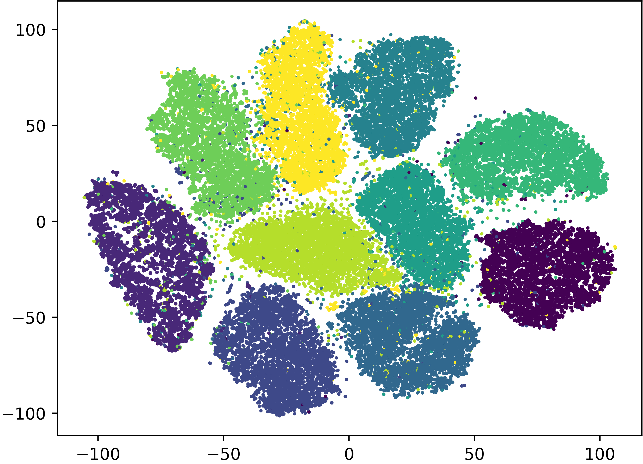
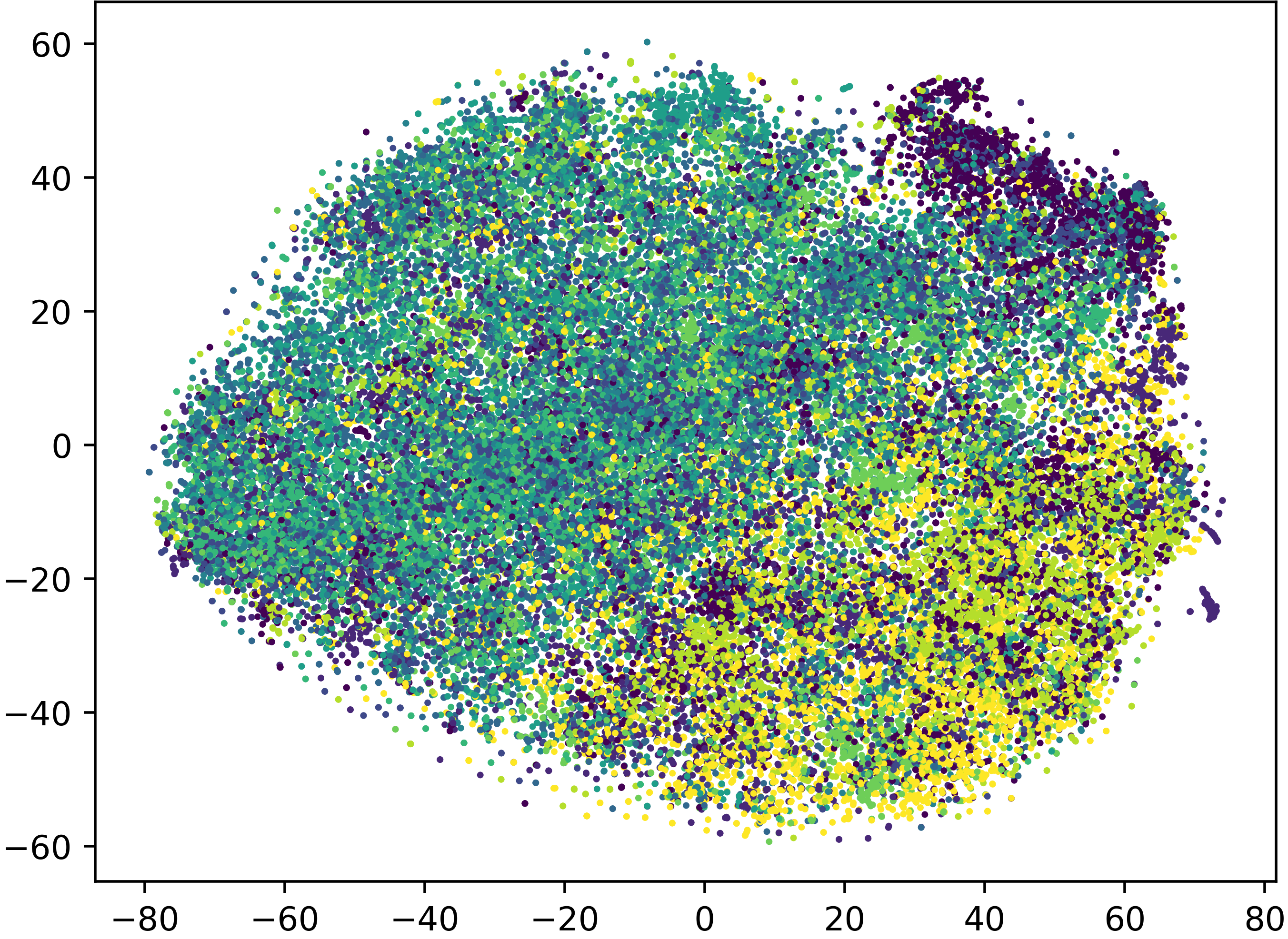
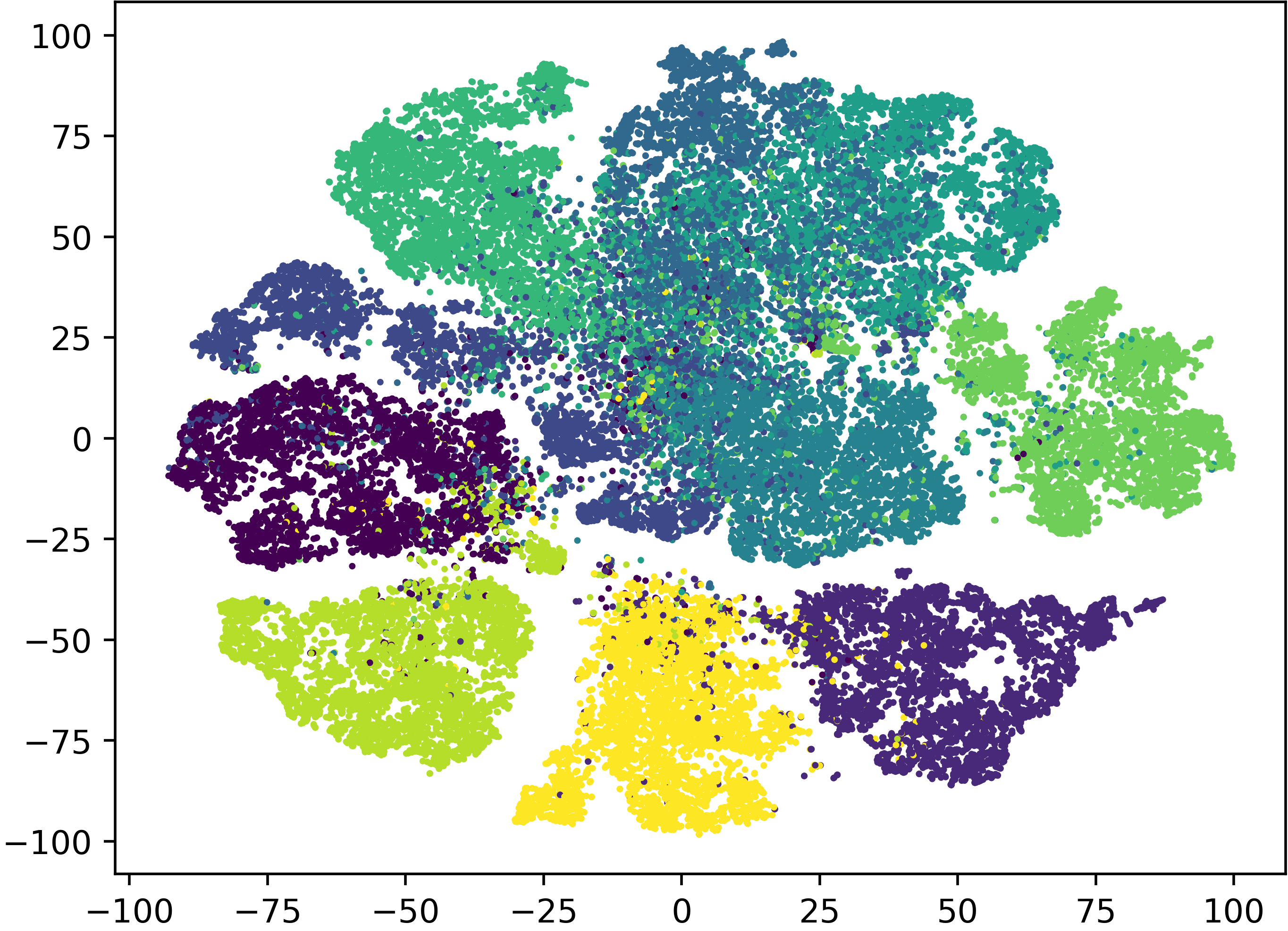
Provided dimensional collapse does not occur, a fundamental unresolved question surrounding many feature learning methods is: why do they work so well at producing embeddings that uncover key features and patterns in data sets? As a simple example, consider fig. 1. In fig. 1(a) and fig. 1(b) we show t-SNE (Van der Maaten & Hinton, 2008) visualizations of the MNIST (Deng, 2012) and Cifar-10 (Krizhevsky et al., 2009) data sets, respectively, using their pixel representations. We can see that visual features are not required on MNIST, which is highly preprocessed, while for Cifar-10 the pixel representations are largely uninformative, and feature representations are essential. In fig. 1(c) we show a t-SNE visualization of the latent embedding of the SimCLR method applied to Cifar-10, which indicates that SimCLR has uncovered a strong clustering structure in Cifar-10 that was not present in the pixel representation.
The goal of this paper is to provide a framework that can begin to address this question, and in particular, to explain fig. 1. To do this, we assume the data follows a corruption model, where the observed data is derived from some clean data with distribution that is highly structured or clustered in some way (e.g., follows the manifold assumption with a clustered density). The observed data is then obtained by applying transformations at random from a set of augmentations to the clean data points (i.e., taking different views of the data), producing a corrupted distribution . The main question that motivated our work is that of understanding what properties of the original clean data distribution can be uncovered by unsupervised contrastive feature learning techniques? That is, once an invariant feature map is learned, is the latent distribution similar in any to the clean distribution , or can it be used to deduce any geometric or topological properties of ?
This paper has two main contributions. For simplicity we focus on SimCLR, and indicate in the appendix how our results extend to other techniques.
-
1.
We show minimizing the SimCLR contrastive learning loss is not sufficient to recover information about . In particular, there are invariant minimizers of the SimCLR loss that are completely independent of the data distributions and . In the extreme case, the original clean data may be highly clustered, while the latent distribution has a minimizer that is the uniform distribution.
-
2.
To understand the success of contrastive learning, it is necessary to analyze the neural network training dynamics induced by gradient descent on the SimCLR loss. Using the neural kernel approach, we show that clusterability structures in strongly affect the training dynamics and can remain present in the latent distribution for a long time, even if gradient descent converges to a trivial minimizer.
Our work complements research on dimension collapse in contrastive learning (Jing et al., 2021; Zhang et al., 2022a; Shen et al., 2022; Li et al., 2022), as our findings hold even without collapse. We also highlight recent work (Meng & Wang, 2024) on the training dynamics of contrastive learning through a continuum limit PDE. Other related works, such as (HaoChen et al., 2021; Balestriero & LeCun, 2022), provide guarantees for downstream tasks like semi-supervised learning by studying the alignment between class-membership clusters and an ”augmentation graph.” Our paper complements these by examining when this alignment holds in contrastive learning.
Outline: In section 2 we overview contrastive learning, and our corruption model for the data. In section 3 we derive and study the optimality conditions for the SimCLR loss, and give conditions for stationary points. In section 4 we study the neural dynamics of training SimCLR for a one-hidden layer neural network.
2 Contrastive learning
We describe here our model for corrupted data in the setting of contrastive learning, and a reformulation of the SimCLR loss that is useful or our analysis. Let be a data distribution in . Let be a set of transformation functions that is measurable such that, for a given , represents a perturbation of , such as a data augmentation (e.g., cropping and image, etc.). Let denote the distribution obtained by perturbing with the perturbations defined in . That is, we choose a probability distribution over the perturbations, and samples from are generated by sampling and , and taking the composition .
We treat as the original clean data, which is not observable, while the perturbed distribution is how the data is presented. Our goal is to understand whether contrastive learning can recover information about the original data , provided the distribution of augmentations is known.
Ostensibly, the objective of contrastive learning is to identify an embedding function that is invariant to the set of transformations . Provided such an invariant map is identified, pushes forwards both and to the same latent distributions, that is
As a result, the desirable map is not only invariant to perturbations from but also successfully retrieves the unperturbed data , ensuring that the embedded distribution serves as a pure feature representation of the given data. However, it is far from clear how and are related, and whether any interesting structures in (such as clusterability) are also present in .
For instance, if represents image data, contrastive learning aims to discover a feature distribution that remains invariant to transformations such as random translation, rotation, cropping, Gaussian blurring, and others. Figure 2 illustrates the mapping and . As a result, this feature distribution effectively captures the essential characteristics of the data without being influenced by these perturbations. These feature distributions are often leveraged in downstream tasks such as classification, clustering, object detection, and retrieval, where they achieve state-of-the-art performance (Le-Khac et al., 2020).
To achieve this, a cost function is designed to bring similar points closer and push dissimilar points apart through the embedding map, using attraction and repulsion forces. A popular example is the Normalized Temperature-Scaled Cross-Entropy Loss (NT-Xent loss) introduced by Chen et al. (2020), which leads to the optimization problem
| (1) |
where is a probability distribution on , which is assumed to be a measurable space, is a given parameter, and is a function measuring the similarity between two embedded points with in defined as:
| (2) |
The denominator inside the log function acts as an attraction force between perturbed points from the same sample , while minimizing the numerator acts as a repulsion force between points from different samples and . Thus, the minimizer of the cost is expected to exhibit invariance under the group of perturbation functions from .
| (3) |
The repulsion force prevents dimensional collapse, where the map sends every sample to a constant: for all .
Our first observation is that the NT-Xent loss becomes independent of the data distribution once is invariant, and so the latent distribution for an invariant minimizer may be completely unrelated to the input data.
Proposition 2.1.
The result in Proposition 2.1 shows that minimizing the NT-Xent cost with respect to an embedding map, once the map is invariant, is equivalent to minimizing over the probability distribution in the latent space. This minimization is completely independent of the input data distribution . A similar phenomenon is observed in other unsupervised learning models like VICReg (Bardes et al., 2021) and BYOL (Grill et al., 2020), with a similar derivation provided in the appendix.
Next, we will analyze the NT-Xent loss by studying its minimizer and the dynamics of gradient descent. To avoid issues with the nondifferentiability of angular similarity and the nonuniqueness of solutions (e.g., is also a minimizer for any ), we reformulate the loss to simplify the analysis. This leads to the generalized formulation of the NT-Xent loss in equation 1.
Definition 2.1.
The cost function we consider for contrastive learning is
| (4) |
where is a nondecreasing function, is a constraint set, and is defined as
| (5) |
where is a differentaible similarity function that is maximized at .
The formulation in eq. 4 generalizes the original formulation in eq. 1 by removing the indicator function , as the effect of this function becomes negligible when a large is considered. Furthermore, the generalized formulation introduces a differentaible similarity function. This simplifies the analysis of the minimizer in the variational formulation. The generalized formulation can easily be related to the original cost function in eq. 1 by setting , and defining . Then, the similarity function retains the same interpretation as angular similarity . This is because, if lies on the unit sphere in , and so
where . The consideration of the constraint also resolves the issue in eq. 1, where , for any , could be a minimizer of eq. 1. Thus, in the end, the introduced formulation in eq. 4 remains fundamentally consistent with the original NT-Xent cost structure.
3 Optimality condition
In this section, we aim to find the optimality condition for eq. 4 and analyze properties of the minimizers. Our first result provides the first order optimality conditions.
Proposition 3.1.
The first optimality condition of the problem eq. 4 takes the form
| (6) |
for all such that where , and .
If is invariant to the perturbation in , then the gradient of takes the form
| (7) |
Using the first optimality condition described in Proposition 3.1, we can characterize the minimizer of the NT-Xent loss in eq. 4. The following theorem describes the possible local minimizers of eq. 4, considering the constraint set defined as .
Theorem 3.2.
Given a data distribution , let be an invariant map such that the embedded distribution is a symmetric discrete measure satisfying
| (8) |
for all and for all anti-symmetric functions such that . Then, is a stationary point of eq. 4 in .
Remark 3.1.
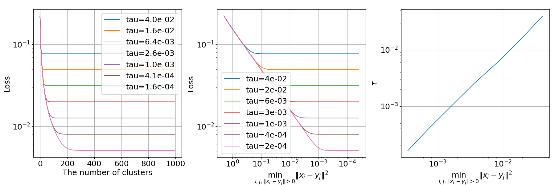
Examples of the embedded distribution in Theorem 3.2 include a discrete measure, , with points evenly distributed on , or all points mapped to a single point, . Figure 3 shows loss plots for different embedded distributions, , with points evenly distributed on , illustrating how each stationary point relates to the loss.
The first plot shows the loss decreasing with the number of clusters, leveling off after a certain point. The second plot shows the loss decreasing as the minimum squared distance between cluster points narrows, plateaus once a threshold is reached. Both suggest that increasing the number of clusters or using a uniform distribution on minimizes the NT-Xent loss. Additionally, increasing the number of points and decreasing further reduces the loss. The third plot reveals a linear relationship between and the threshold for the minimum squared distance, offering insight into the optimal cluster structure for minimizing the loss at a given .
Remark 3.2.
Theorem 3.2 is related to the result from Wang & Isola (2020), where the authors studied local minimizers by minimizing the repulsive force under the assumption of an invariant feature map. They showed that, asymptotically, the uniform distribution on becomes a local minimizer as the number of negative points increases. Our result extends this by offering a more general, both asymptotic and non-asymptotic characterization of local minimizers, broadening their findings.
It follows from Theorem 3.2 that gradient descent on the NT-Xent loss can lead to solutions that are completely independent of the original data distribution . For instance, if has some underlying cluster structure, with multiple clusters, there are minimizers of the NT-Xent loss, i.e., an invariant map , that map onto an arbitrary distribution in the latent space, completely independent of the clustering structure of . However, in practice, when the map is parameterized using neural networks, and trained with gradient descent on , it is very often observed that the clustering structure of the original data distribution emerges in the latent space (see fig. 1). In fact, our results in section 4 show that this is true even if we initialize gradient descent very poorly, starting with an invariant mapping to the uniform distribution !
Although the contrastive loss has minimizers that ignore the data distribution , leading to poor results, contrastive learning often achieves excellent performance in practice. This suggests that the neural network’s parameterization and gradient descent optimization are selecting a good minimizer for , producing well-clustered distributions in the latent space. To understand this, we will analyze the dynamics of neural network optimization during training in the following sections.
4 Optimization of Neural Networks
Here, we study contrastive learning through the lens of the associated neural network training dynamics, which illustrates how the data distribution enters the latent space through the neural kernel. In this section, we use the notation .
4.1 Gradient flow from neural network parameters
Let be a vector of neural network parameters, be data samples, and be an embedding function where each function is a scalar function for . Consider a loss function with respect to :
| (9) |
Let be a vector of neural network parameters as a function of time . The gradient descent flow can be expressed as
Due to the highly non-convex nature of , this gradient flow is difficult to analyze. By shifting the focus to the evolution of the neural network’s output on the training data over time, rather than the weights, we can derive an alternative gradient flow with better properties for easier analysis. The following proposition outlines this gradient flow derived from the loss function . The proof of the proposition is provided in the appendix.
Proposition 4.1.
Let be a vector of neural network parameters as a function of time . Consider a set of data samples . Define a matrix function such that
| (10) |
Let denote the -th column of . Then, satisfies the following ordinary differential equation (ODE) for each :
| (11) |
where the kernel matrix is given by
| (12) |
Remark 4.1.
We remark that the viewpoint in proposition 4.1, of lifting the training dynamics from the neural network weights to the function space setting, is the same that is taken by the Neural Tangent Kernel (NTK) Jacot et al. (2018). The difference here is that we do not consider an infinite width neural network, and we evaluate the kernel function on the training data, so the results are stated with kernel matrices that are data dependent (which is important in what follows). In fact, it is important to note that proposition 4.1 is very general and holds for any parameterization of , e.g., we have so far not used that is a neural network.
Remark 4.2.
The training dynamics in the absence of a neural network can be expressed as
| (13) |
where is set to be identity matrices. In contrast to eq. 11, the above expression shows that the training dynamics on the -th point are influenced solely by the gradient of the loss function at , and there is no mixing of the data via the neural kernel (since here it is the identity matrix).
Using proposition 4.1 we can study the invariance-preserving properties (or lack thereof) of gradient descent with and without the neural network kernel.
Theorem 4.2.
Consider the gradient descent iteration from a gradient flow without a neural network in eq. 13, where for all , and
| (14) |
with as the step size. If is invariant to perturbations from , as defined in eq. 17, then remains invariant for all gradient descent iterations.
On the other hand, in the case of a gradient descent iteration from eq. 10,
| (15) |
the invariance of at the -th iteration holds only if is invariant at the -th iteration and additionally satisfies the condition for all and .
Theorem 4.2 contrasts optimization with and without neural networks. In standard gradient descent (eq. 14), the map remains invariant if it is initially invariant. In contrast, with the neural kernel in eq. 15, even if starts invariant, an additional condition on is needed to maintain invariance. Since this condition is not guaranteed be satisfied throughout the iterations, the optimization can cause to lose invariance, resulting in different dynamics compared to standard gradient descent.
Many other works have shown that the neural kernel imparts significant changes on the dynamics of gradient descent. For example, Xu et al. (2019a; b) established the frequency principle, showing that the training dynamics of neural networks are significantly biased towards low frequency information, compared to vanilla gradient descent.
4.2 Studying a clustered dataset
In this section, we explore how the neural network kernel in eq. 12 influences the gradient flow on the contrastive learning loss. For clarity, we use a simplified setting that is straightforward enough to provide insights into the neural network’s impact on the optimization process. Although simplified, the setting can be easily generalized to extend these insights to broader contexts.
Dataset Description
Consider a data distribution , where is a -dimensional compact submanifold in , and a noisy data distribution defined by
where represents noise (or perturbation) applied to in the orthogonal direction to .
For simplicity, assume that
Now, let’s impose a clustered structure on the dataset. Given a dataset with samples i.i.d. from the noisy distribution , we assume that the data is organized into () clusters. Let be points in such that if , and otherwise. Suppose the data samples are arranged such that for each ,
| (16) |
where and is a random variable (i.e., noise) and for some positive constant . This setup ensures that each data point lies within a ball of radius centered at one of the points , effectively representing the dataset as clusters.
Embedding Map Description
Let be an embedding map parameterized by a neural network, such that , where is a vector of neural network parameters. We assume that at , satisfies
| (17) |
for all , where is an arbitrary map. Consequently, this embedding map is invariant under the following perturbations: for and ,
Thus, is an invariant to the perturbation from . This serves to initialize the embedding map to be an invariant map that is unrelated to the data distribution . This is in some sense the “worst case” initialization, where no information from the data distribution has been imbued upon the latent distribution. The goal is to examine what happens when using this as the initialization for training. As we will see below, the neural kernel always injects information from into the optimization procedure, and can even help recover from poor initializations.
4.2.1 Properties of the embedding map
In this section, we derive the explicit formulations for the gradients and the kernel matrix defined in eq. 12, within the setting described in Section 4.2. We examine the training dynamics of eq. 10 to understand how they are influenced by the neural network kernel matrix and the dataset’s clustering structure. Specifically, we consider the embedding map parameterized by a one-hidden-layer fully connected neural network:
| (18) |
where is a constant matrix defined as
| (19) |
where and represent the -dimensional vectors of ones and zeros, respectively. Additionally, is the weight matrix, and is a differentiable activation function applied element-wise.
Note that acts as an averaging matrix that, when multiplied by the -dimensional vector , produces a -dimensional vector. Furthermore, we assume that the parameters of are uniformly bounded, such that there exists a constant with for all , , and .
Remark 4.3.
In many contrastive learning studies, the neural network is trained, but the last layer is discarded when retrieving feature representations. Research Bordes et al. (2023); Gui et al. (2023); Wen & Li (2022) shows that discarding the last layer can improve feature quality. While we do not consider this in our analysis for simplicity, exploring its impact on training dynamics is an interesting direction for future work.
Based on the definitions of kernel matrices in eq. 12 and the neural network function in eq. 18, the following proposition provides the explicit kernel formula.
Proposition 4.3.
From Proposition 4.3, as done in NTK paper (Jacot et al., 2018), one can consider how the kernel converges as the width of the neural network approaches infinity, i.e., as in eq. 18. The following proposition shows the formulation of the limiting kernel in the infinite-width neural network.
Proposition 4.4.
Suppose the weight matrix satisfies that each row vector , for , consists of independent and identically distributed random variables in with a Gaussian distribution. Also, suppose the activation function is . Then, as , the kernel matrix converges to , where
Using the kernel matrix defined in Proposition 4.3, the following theorem presents the explicit form of the gradient flows in terms of the clustering structure and the neural network parameters.
Theorem 4.5.
Let the dataset to be clustered be as described in eq. 16. Define a function such that if is from the cluster point . Then, the gradient flow formulation takes the form
| (21) |
where () is a diagonal matrix where each diagonal entry () is defined as
Similar to Proposition 4.4, one can consider the gradient flow formulation in the limit of infinite width, i.e., as . The following corollary provides the explicit form of the neural network gradient flow in the infinite width case.
Corollary 4.6.
Under the same conditions as in Proposition 4.4 and Theorem 4.5, if the width approaches infinity, i.e., , then the gradient formulation in eq. 21 becomes
Remark 4.4.
The results from Theorem 4.5 and Proposition 4.4 show the explicit gradient flow under the clustering setting, where the gradient is scaled by the ratio of each cluster’s size represented as . This means that if a certain cluster contains only a small number of points, the gradient at those points could be negligible compared to the gradient from a cluster with a larger number of points, which may result in the failure to capture the smaller cluster effectively. This result aligns well with the findings in Assran et al. (2022), where the authors show that semi-supervised methods, including contrastive learning, tend to perform worse with imbalanced class data and work better with uniform class distributions.
The formulations of the gradient flow in Theorem 4.5 and Corollary 4.6 can be viewed as a modification of the training dynamics of the vanilla gradient flow in eq. 13, altered in such a way as to steer the iterations towards a stationary solution that is both invariant to perturbations and influenced by the dataset’s geometry. Specifically, the first term in eq. 21 shows that for every data point that originates from the same cluster, the gradient will be the same, with an error of order . This means that if the neural network is initialized randomly, such that the embeddings from the feature map are completely random in the latent space, the gradient at points from the same cluster in the embedded space will follow the same direction. This results in training dynamics that lead to embeddings that exhibit the data’s clustering structure.
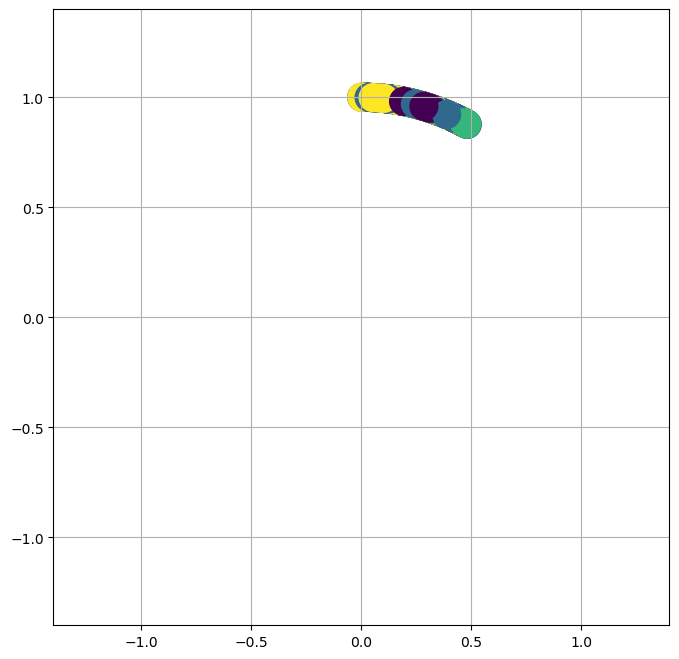
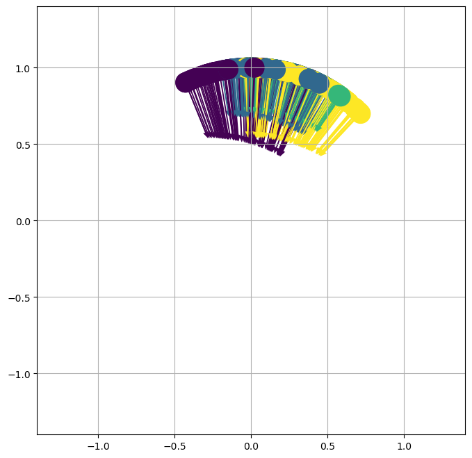
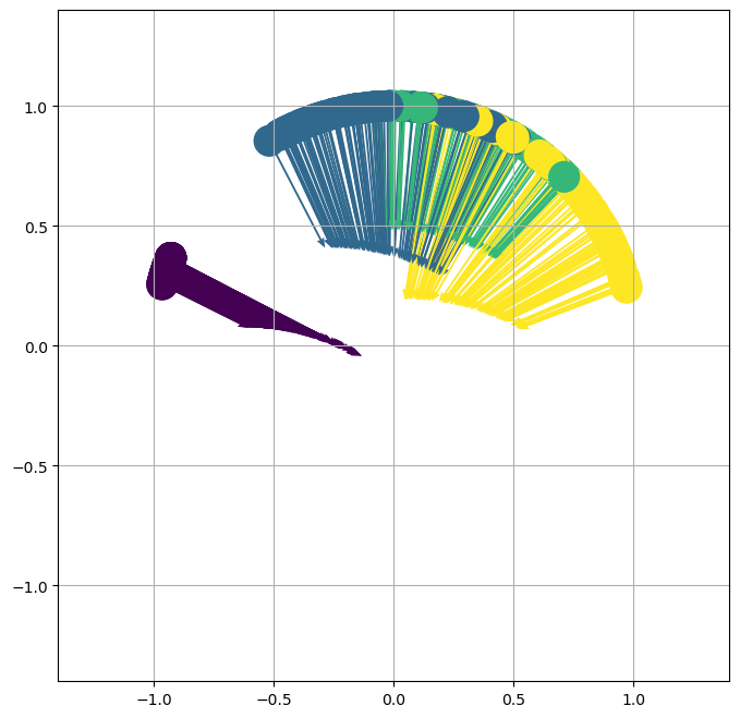
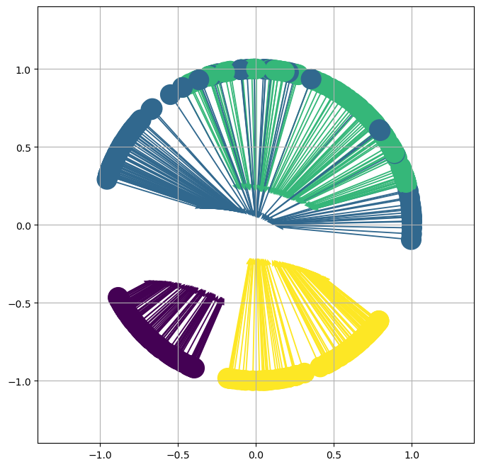
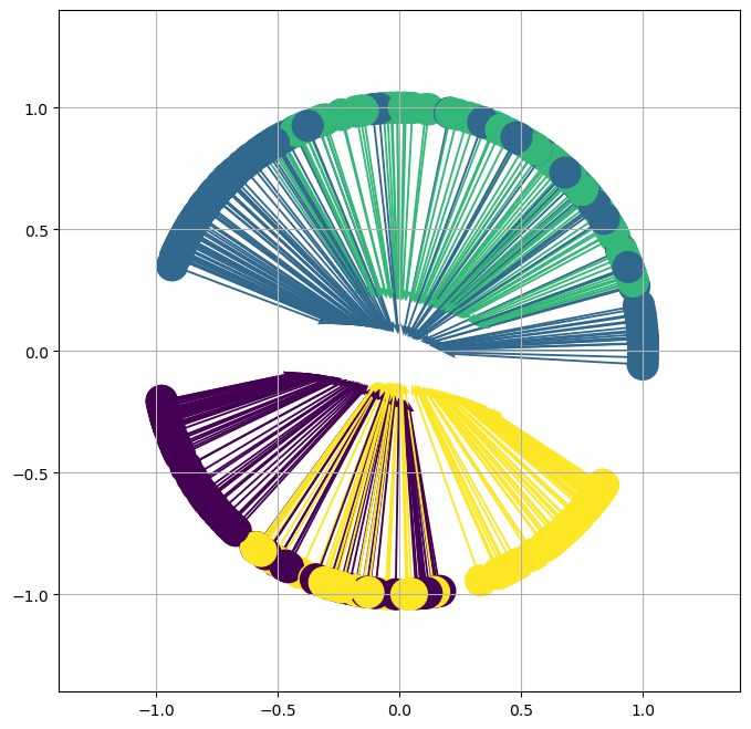
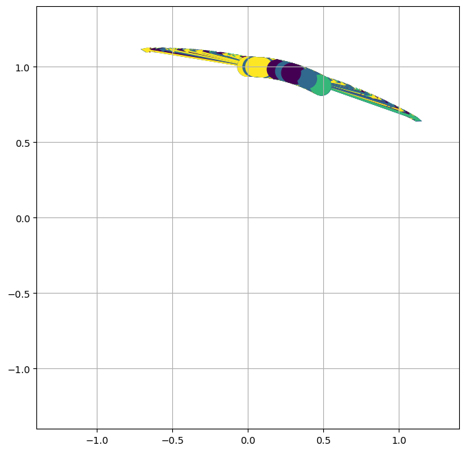
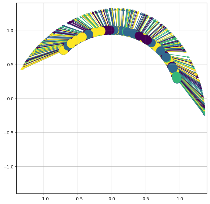
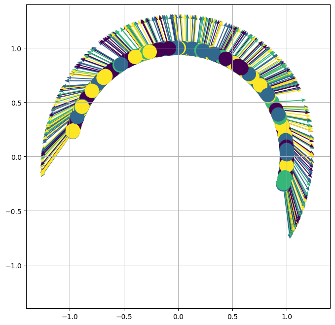
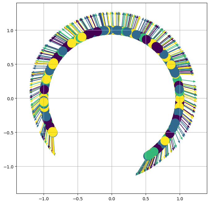
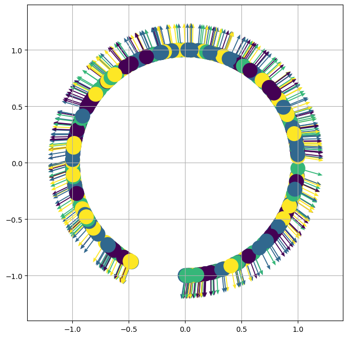
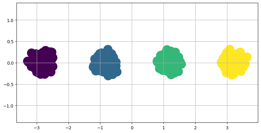
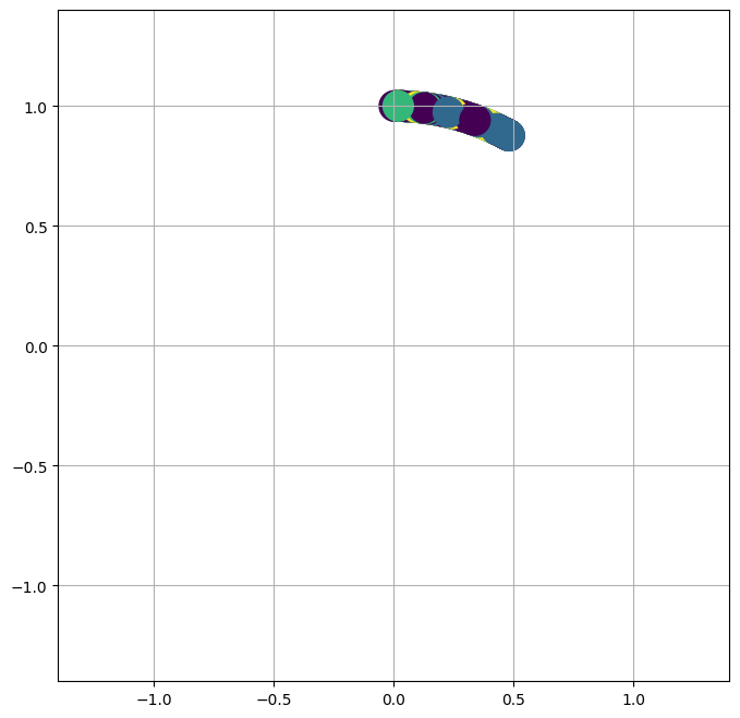
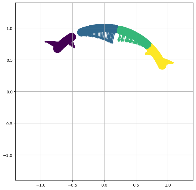
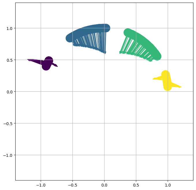
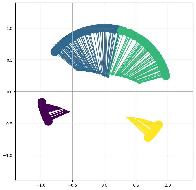
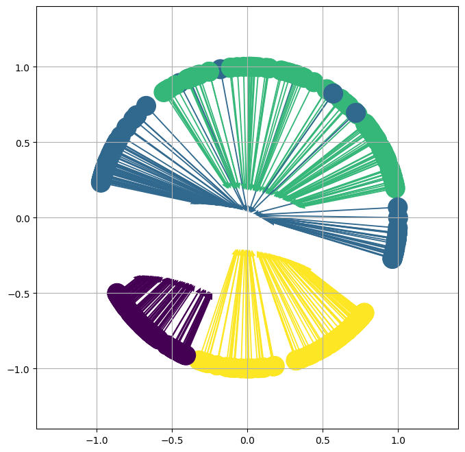
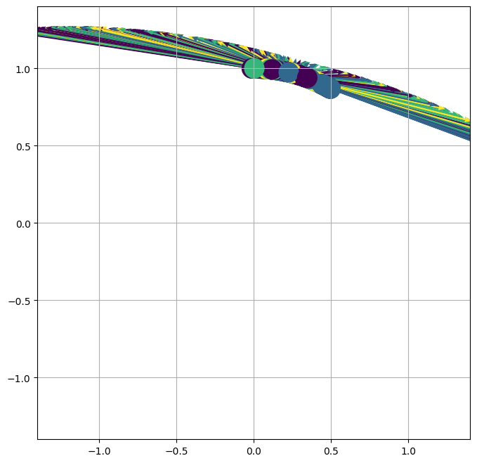
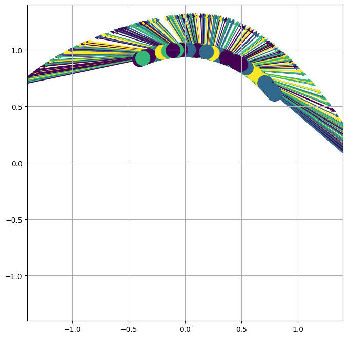
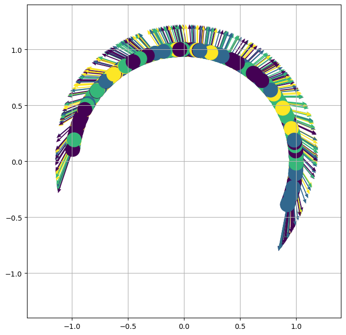
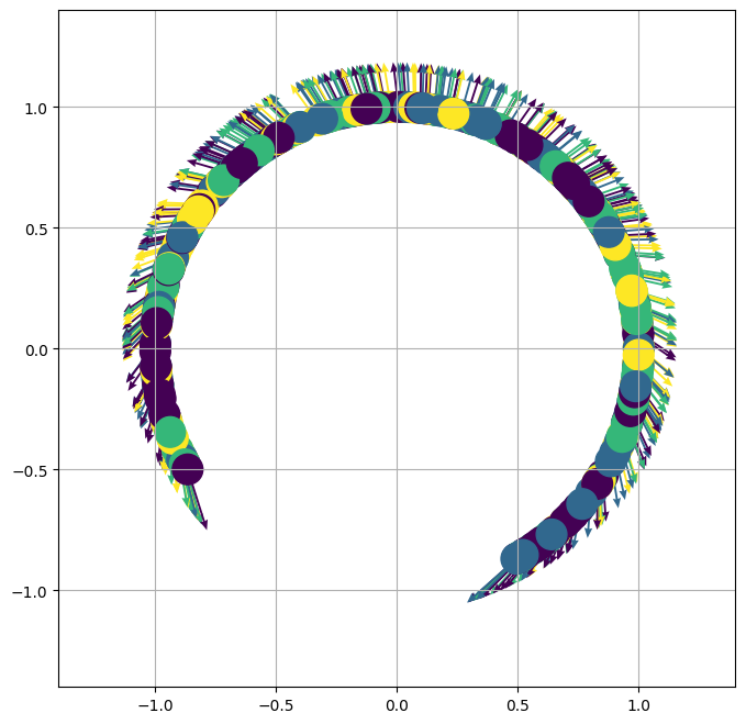
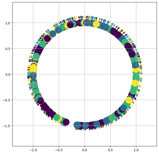
This behavior is reflected in the numerical results in Figure 5, where a 2D dataset with four clusters located along the -axis at (purple), (blue), (green), and (yellow) is analyzed. The arrow at each point indicates the negative gradient computed at that point. In the figure, the number of iterations is chosen differently for each training dynamic (with and without neural network optimization) because the neural network kernel matrix affects the training dynamics, causing the models to converge at different speeds. The iterations in the visualization are selected to best capture and effectively depict the evolution of the feature distribution during training. Furthermore, both figures stabilize after a certain number of iterations: the first (b-f), with neural network optimization, after 200 iterations, and the second (g-k), without it, after 1,000 iterations.
The training dynamics show that, despite starting from a random initialization without any initial clustering structure, data points from the same cluster follow a similar gradient. This shared gradient, relative to their respective clusters, drives the separation of data points from different clusters in the early iterations. By iteration 15, the clustering structure of the input data is already preserved in the embedded distribution, after just a few iterations. In contrast, without neural network optimization, the embedded data points spread out and eventually form a uniform distribution on a sphere, disregarding the input data’s cluster structure. This result aligns with the theoretical findings in Theorem 3.2, which suggest that the gradient of the loss function is independent of the input data’s structure.
5 Conclusion and Future Work
We have studied the SimCLR contrastive learning problem from the perspective of a variational analysis and through the dynamics of training a neural network to represent the embedding function. Our findings strongly suggest that in order to fully understand the representation power of contrastive learning, it is necessary to study the training dynamics of gradient descent, as vanilla gradient descent forgets all information about the data distribution.
The results in this paper are preliminary, and there are many interesting directions for future work. It would be natural to examine a mean field limit (Mei et al., 2018) for the training dynamics, which may shed more light on this phenomenon (e.g., in theorem 4.5). We can also consider an infinite width neural network, as is done in the NtK setting, in theorem 4.5 to attempt to rigorously establish convergence of the training dynamics. It would also be interesting to explore applications of these techniques to other deep learning methods.
Acknowledgments and Disclosure of Funding
WL acknowledges funding from the National Institute of Standards and Technology (NIST) under award number 70NANB22H021, and JC was supported by NSF-DMS:1944925, NSF-CCF:2212318, the Alfred P. Sloan Foundation, and the Albert and Dorothy Marden Professorship.
References
- Assran et al. (2022) Mahmoud Assran, Randall Balestriero, Quentin Duval, Florian Bordes, Ishan Misra, Piotr Bojanowski, Pascal Vincent, Michael Rabbat, and Nicolas Ballas. The hidden uniform cluster prior in self-supervised learning. arXiv preprint arXiv:2210.07277, 2022.
- Bachman et al. (2019) Philip Bachman, R Devon Hjelm, and William Buchwalter. Learning representations by maximizing mutual information across views. Advances in neural information processing systems, 32, 2019.
- Balestriero & LeCun (2022) Randall Balestriero and Yann LeCun. Contrastive and non-contrastive self-supervised learning recover global and local spectral embedding methods. Advances in Neural Information Processing Systems, 35:26671–26685, 2022.
- Bardes et al. (2021) Adrien Bardes, Jean Ponce, and Yann LeCun. Vicreg: Variance-invariance-covariance regularization for self-supervised learning. arXiv preprint arXiv:2105.04906, 2021.
- Bordes et al. (2023) Florian Bordes, Randall Balestriero, Quentin Garrido, Adrien Bardes, and Pascal Vincent. Guillotine regularization: Why removing layers is needed to improve generalization in self-supervised learning. Transactions on Machine Learning Research, 2023. ISSN 2835-8856. URL https://openreview.net/forum?id=ZgXfXSz51n.
- Chen et al. (2020) Ting Chen, Simon Kornblith, Mohammad Norouzi, and Geoffrey Hinton. A simple framework for contrastive learning of visual representations. In International conference on machine learning, pp. 1597–1607. PMLR, 2020.
- Chicco (2021) Davide Chicco. Siamese neural networks: An overview. Artificial neural networks, pp. 73–94, 2021.
- Deng (2012) Li Deng. The mnist database of handwritten digit images for machine learning research. IEEE Signal Processing Magazine, 29(6):141–142, 2012.
- Dosovitskiy et al. (2014) Alexey Dosovitskiy, Jost Tobias Springenberg, Martin Riedmiller, and Thomas Brox. Discriminative unsupervised feature learning with convolutional neural networks. Advances in neural information processing systems, 27, 2014.
- Grill et al. (2020) Jean-Bastien Grill, Florian Strub, Florent Altché, Corentin Tallec, Pierre Richemond, Elena Buchatskaya, Carl Doersch, Bernardo Avila Pires, Zhaohan Guo, Mohammad Gheshlaghi Azar, et al. Bootstrap your own latent-a new approach to self-supervised learning. Advances in neural information processing systems, 33:21271–21284, 2020.
- Gui et al. (2023) Yu Gui, Cong Ma, and Yiqiao Zhong. Unraveling projection heads in contrastive learning: Insights from expansion and shrinkage. arXiv preprint arXiv:2306.03335, 2023.
- Hadsell et al. (2006) Raia Hadsell, Sumit Chopra, and Yann LeCun. Dimensionality reduction by learning an invariant mapping. In 2006 IEEE computer society conference on computer vision and pattern recognition (CVPR’06), volume 2, pp. 1735–1742. IEEE, 2006.
- HaoChen et al. (2021) Jeff Z HaoChen, Colin Wei, Adrien Gaidon, and Tengyu Ma. Provable guarantees for self-supervised deep learning with spectral contrastive loss. Advances in Neural Information Processing Systems, 34:5000–5011, 2021.
- Jacot et al. (2018) Arthur Jacot, Franck Gabriel, and Clément Hongler. Neural tangent kernel: Convergence and generalization in neural networks. Advances in neural information processing systems, 31, 2018.
- Ji et al. (2023) Wenlong Ji, Zhun Deng, Ryumei Nakada, James Zou, and Linjun Zhang. The power of contrast for feature learning: A theoretical analysis. Journal of Machine Learning Research, 24(330):1–78, 2023.
- Jing et al. (2021) Li Jing, Pascal Vincent, Yann LeCun, and Yuandong Tian. Understanding dimensional collapse in contrastive self-supervised learning. arXiv preprint arXiv:2110.09348, 2021.
- Khosla et al. (2020) Prannay Khosla, Piotr Teterwak, Chen Wang, Aaron Sarna, Yonglong Tian, Phillip Isola, Aaron Maschinot, Ce Liu, and Dilip Krishnan. Supervised contrastive learning. Advances in neural information processing systems, 33:18661–18673, 2020.
- Kim et al. (2021) Byoungjip Kim, Jinho Choo, Yeong-Dae Kwon, Seongho Joe, Seungjai Min, and Youngjune Gwon. Selfmatch: Combining contrastive self-supervision and consistency for semi-supervised learning. arXiv preprint arXiv:2101.06480, 2021.
- Krizhevsky et al. (2009) Alex Krizhevsky, Geoffrey Hinton, et al. Learning multiple layers of features from tiny images. 2009.
- Le-Khac et al. (2020) Phuc H Le-Khac, Graham Healy, and Alan F Smeaton. Contrastive representation learning: A framework and review. Ieee Access, 8:193907–193934, 2020.
- Lee et al. (2022) Doyup Lee, Sungwoong Kim, Ildoo Kim, Yeongjae Cheon, Minsu Cho, and Wook-Shin Han. Contrastive regularization for semi-supervised learning. In Proceedings of the IEEE/CVF conference on computer vision and pattern recognition, pp. 3911–3920, 2022.
- Li et al. (2022) Alexander C Li, Alexei A Efros, and Deepak Pathak. Understanding collapse in non-contrastive siamese representation learning. In European Conference on Computer Vision, pp. 490–505. Springer, 2022.
- Li et al. (2021) Junnan Li, Caiming Xiong, and Steven CH Hoi. Comatch: Semi-supervised learning with contrastive graph regularization. In Proceedings of the IEEE/CVF international conference on computer vision, pp. 9475–9484, 2021.
- Mei et al. (2018) Song Mei, Andrea Montanari, and Phan-Minh Nguyen. A mean field view of the landscape of two-layer neural networks. Proceedings of the National Academy of Sciences, 115(33):E7665–E7671, 2018.
- Meng & Wang (2024) Linghuan Meng and Chuang Wang. Training dynamics of nonlinear contrastive learning model in the high dimensional limit. IEEE Signal Processing Letters, 2024.
- Mialon et al. (2023) Grégoire Mialon, Quentin Garrido, Hannah Lawrence, Danyal Rehman, Yann LeCun, and Bobak Kiani. Self-supervised learning with lie symmetries for partial differential equations. Advances in Neural Information Processing Systems, 36:28973–29004, 2023.
- Oord et al. (2018) Aaron van den Oord, Yazhe Li, and Oriol Vinyals. Representation learning with contrastive predictive coding. arXiv preprint arXiv:1807.03748, 2018.
- Shen et al. (2022) Kendrick Shen, Robbie M Jones, Ananya Kumar, Sang Michael Xie, Jeff Z HaoChen, Tengyu Ma, and Percy Liang. Connect, not collapse: Explaining contrastive learning for unsupervised domain adaptation. In International conference on machine learning, pp. 19847–19878. PMLR, 2022.
- Singh (2021) Ankit Singh. Clda: Contrastive learning for semi-supervised domain adaptation. Advances in Neural Information Processing Systems, 34:5089–5101, 2021.
- Tian et al. (2020) Yonglong Tian, Chen Sun, Ben Poole, Dilip Krishnan, Cordelia Schmid, and Phillip Isola. What makes for good views for contrastive learning? Advances in neural information processing systems, 33:6827–6839, 2020.
- Van der Maaten & Hinton (2008) Laurens Van der Maaten and Geoffrey Hinton. Visualizing data using t-sne. Journal of machine learning research, 9(11), 2008.
- Wang & Isola (2020) Tongzhou Wang and Phillip Isola. Understanding contrastive representation learning through alignment and uniformity on the hypersphere. In International conference on machine learning, pp. 9929–9939. PMLR, 2020.
- Wen & Li (2022) Zixin Wen and Yuanzhi Li. The mechanism of prediction head in non-contrastive self-supervised learning. Advances in Neural Information Processing Systems, 35:24794–24809, 2022.
- Xu et al. (2019a) Zhi-Qin John Xu, Yaoyu Zhang, Tao Luo, Yanyang Xiao, and Zheng Ma. Frequency principle: Fourier analysis sheds light on deep neural networks. arXiv preprint arXiv:1901.06523, 2019a.
- Xu et al. (2019b) Zhi-Qin John Xu, Yaoyu Zhang, and Yanyang Xiao. Training behavior of deep neural network in frequency domain. In Neural Information Processing: 26th International Conference, ICONIP 2019, Sydney, NSW, Australia, December 12–15, 2019, Proceedings, Part I 26, pp. 264–274. Springer, 2019b.
- Yang et al. (2022) Fan Yang, Kai Wu, Shuyi Zhang, Guannan Jiang, Yong Liu, Feng Zheng, Wei Zhang, Chengjie Wang, and Long Zeng. Class-aware contrastive semi-supervised learning. In Proceedings of the IEEE/CVF Conference on Computer Vision and Pattern Recognition, pp. 14421–14430, 2022.
- Zhang et al. (2022a) Chaoning Zhang, Kang Zhang, Chenshuang Zhang, Trung X Pham, Chang D Yoo, and In So Kweon. How does simsiam avoid collapse without negative samples? a unified understanding with self-supervised contrastive learning. arXiv preprint arXiv:2203.16262, 2022a.
- Zhang et al. (2022b) Yuhang Zhang, Xiaopeng Zhang, Jie Li, Robert C Qiu, Haohang Xu, and Qi Tian. Semi-supervised contrastive learning with similarity co-calibration. IEEE Transactions on Multimedia, 25:1749–1759, 2022b.
Appendix A Appendix
In the appendix, we present the proofs of that are missing in the main manuscript.
A.1 Interpretation of VICReg and BYOL
In this section, we show that two other popular methods related to deep learning models for learning dataset invariance exhibit a similar phenomenon as shown in Proposition 2.1, namely that the loss function itself is ill-posed. First, consider the VICReg Bardes et al. (2021) loss. Given a data distribution and a distribution for the perturbation functions , VICReg minimizes
where , , and are hyperparameters. The first term ensures the invariance of with respect to perturbation functions from , maintains the variance of each embedding dimension, and regularizes the covariance between pairs of embedded points towards zero. Suppose is an invariant embedding map such that for all . Then, the above minimization problem becomes
Similar to the result in Proposition 2.1, the invariance term vanishes. This minimization can now be expressed as a minimization over the embedded distribution:
This shows that given an invariant map , the minimization problem becomes completely independent of the input data , thus demonstrating the same ill-posedness as the NT-Xent loss in Proposition 2.1.
Now, consider the loss function from BYOL Grill et al. (2020). Given a data distribution and a distribution for the perturbation functions , the loss takes the form
where is an auxiliary function designed to prevent from collapsing all points to a constant in . Similar to the previous case, if we assume an invariant map , the above problem becomes
where the second equality follows from a change of variables. Again, this minimization problem can be written with respect to the embedded distribution as:
This again shows that once the invariant map is considered, the minimization problem becomes completely independent of the input data , highlighting the ill-posedness of the cost function.
A.2 Further analysis of the stationary points of Equation 4
From the modified formulation eq. 4, we can define a minimizer that minimizes the function on a constraint set . The following proposition provides insight into the minimizer of eq. 4. The proof is provided in the appendix.
Proposition A.1.
This proposition describes three different possible local minimizers of eq. 4 that satisfy the Euler-Lagrange equation in eq. 6.
-
1.
Any map that maps to a constant, such that
-
2.
In addition to the condition in eq. 5, suppose the attraction and repulsion similarity functions and satisfy the following properties:
-
(a)
Each function is maximized at 0, where its value is 1.
-
(b)
Each function satisfies and .
Let be a map invariant to . Consider a sequence of maps such that
The limit satisfies the Euler-Lagrange equation eq. 6.
-
(a)
Proof of Proposition A.1.
If is a constant function, it is trivial that it satisfies eq. 6.
Let us prove the second part of the proposition. From the Euler-Lagrange equation in eq. 6, by plugging in and using the fact that is invariant to , the Euler-Lagrange equation can be simplified to
for any . Using the invariance of , we have
| (22) |
Furthermore, by the assumptions on the function ,
Thus, eq. 22 converges to as . This proves the theorem. ∎
A.3 Proof of Theorem 3.2
First, we prove Theorem 3.2, which characterizes the stationary points of the loss function. After the proof, we demonstrate that by considering an additional condition on the direction of the second variation at the stationary points, it is the second variation is strictly positive, thereby showing that the stationary point is a local minimizer under this condition.
Proof of Theorem 3.2.
We consider the following problem:
| (23) |
where is a loss function defined in eq. 4. The problem in eq. 23 can be reformulated as a constrained minimization problem:
By relaxing the the constraint for , we can derive the lower bound such that
Note that since the constraint sets satisfy , the stationary point from from the latter constraint set is also the stationary point of the prior set.
By introducing the Lagrange multiplier for the constraint, we can convert the minimization problem into a minimax problem:
| (24) |
Using the Euler-Lagrange formulation in eq. 6, we can derive the Euler-Lagrange equation for the above problem, incorporating the Lagrange multiplier. To show that is a minimizer of the problem in eq. 24, we need to demonstrate that there exists such that the following equation holds:
for all . Note that since is an invariant map, disappears and . Furthermore, since maps onto , we have for all . Additionally, using the change of variables, we obtain
| (25) |
where is defined as for . Given that the function
is an anti-symmetric function, by the assumption on in eq. 8, the integral on the right-hand side of eq. 25 is constant for all . Therefore, by defining as in eq. 25, this proves the lemma. ∎
Now that we have identified the characteristics required for embedding maps to be stationary points, the next lemma shows that the second variation at this stationary point, in a specific direction , is positive. This demonstrates that the stationary point is indeed a local minimizer along this particular direction.
Lemma A.2.
Fix and define . Let be an embedding map such that the embedded distribution is a discrete measure on , satisfying that the number of points , where is the number of cluster centers and is some positive integer. Moreover, the points satisfy the condition:
| (26) |
Furthermore, let be a positive constant satisfying . Then,
for any satisfying and
| (27) |
Proof.
Let be an invariant embedding map. From the proof of LABEL:proof:cor:mini, the first variation takes the form
The second variation takes the form
For simplicity, let us choose explicit forms for and . The proof will be general enough to apply to any and that satisfy the conditions mentioned in the paper. Let and . With these choice of functions and by the change of variables,
| (28) |
where and . By Jensen’s inequality, we have
Therefore, eq. 28 can be bounded below by
By the assumption on in eq. 26, the above can be written as
| (29) | ||||
If , the second variation becomes , and is therefore nonnegative. Now, suppose . We can bound from below by
| (30) |
Furthermore, from the condition in eq. 27, we have
| (31) |
for some positive constant . Combining eq. 30 and eq. 31, we can bound eq. 29 from below by
By the condition on , the above quantity is strictly greater than zero. This concludes the proof of the lemma.
∎
A.4 Proof of Proposition 4.1
Proof.
The gradient of is given by
| (32) |
where is a gradient of with respect to coordinate. For simplicity of notation, let us denote by
Thus, eq. 32 can be rewritten as
| (33) |
By the definition of the loss function in eq. 9, satisfies the gradient flow such that
| (34) |
Thus, the solution of the above ODE converges to the local minimizer of as grows.
A.5 Proof of Theorem 4.2
Proof.
Consider the gradient descent iterations in eq. 14. Suppose is invariant to the perturbation from at -th iteration, that is we have for all and . We want to show that, given an invariant embedding map , it remains invariant after iteration . From the gradient formulation of the loss function in Proposition 3.1, we have
where .
From the gradient descent formulation in eq. 14, we have
which gives
and since by invariance, this simplifies to
which shows that is invariant for all . Therefore, the embedding map remains invariant throughout the optimization process.
Now, consider the gradient descent iteration with a neural network in eq. 15. Suppose is invariant to perturbations from and satisfies
| (36) |
Denote the kernel matrix function given a perturbation function as
Then, we have
Thus, if is invariant at the -th iteration, it remains invariant. However, note that this result no longer holds if the condition in eq. 36 fails, meaning that is not invariant for -th iteration. This completes the proof. ∎
A.6 Proof of Proposition 4.3
Proof.
We describe the matrices and as follows:
In this notation, and are -dimensional column vectors, and are - and -dimensional row vectors, and and are scalars.
We can write with respect to and .
where the last equality uses the definition of a matrix in eq. 19. By differentiating with respect to , we can derive explicit forms for the gradient of with respect to a weight matrix .
where the row index of nonzero entries ranges from to .
Define an inner product such that for
Now we are ready to show the explicit formula of the inner product .
where is an indicator function that equals if and otherwise. Therefore, the kernel matrix takes the form
∎
Proof of Theorem 4.5.
Using the definition of a function in Theorem 4.5 and using the structure of the dataset in eq. 16, consider and in -th cluster and -th cluster respectively. Since the dataset is sampled from a compactly supported data distribution and given the assumption that the activation function has bounded derivatives, we have
Thus,
Combining all, we can write the kernel matrix as the following
where () is a diagonal matrix defined as
where () is defined as
| (37) |
Thus, from the gradient flow formulation in eq. 10, we have
∎
Appendix B Extra nuemrical results
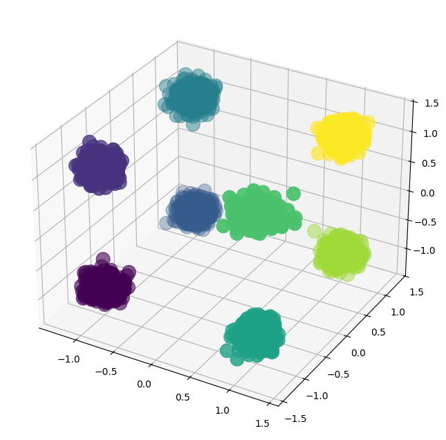
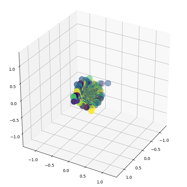
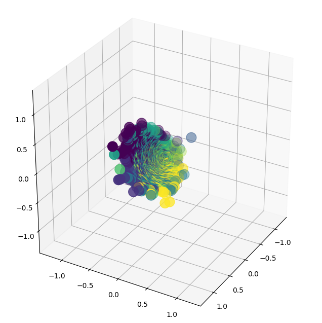
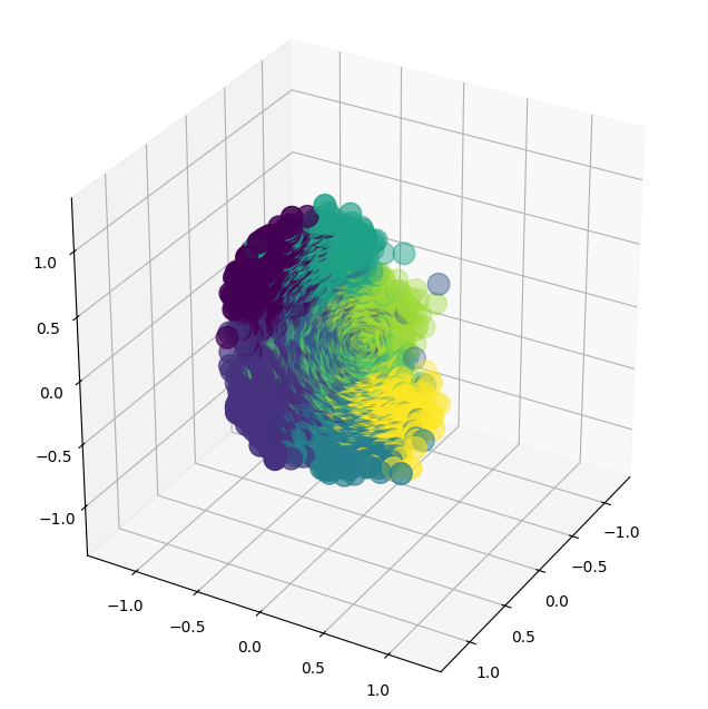
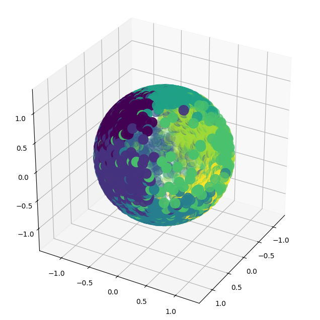
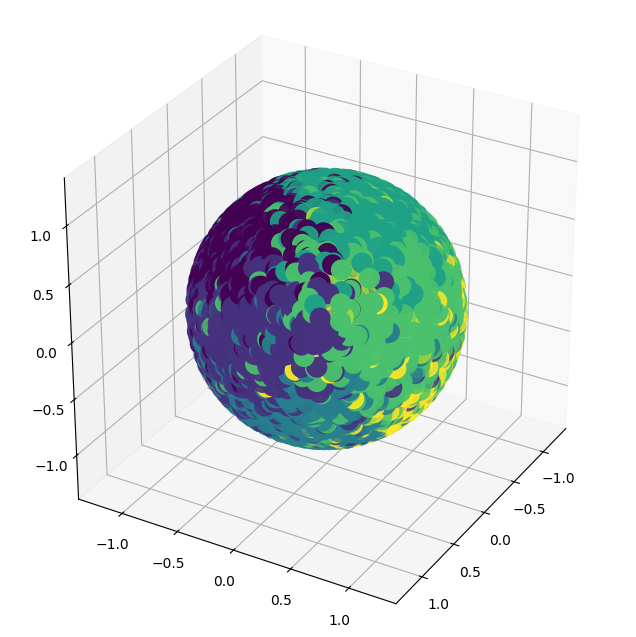
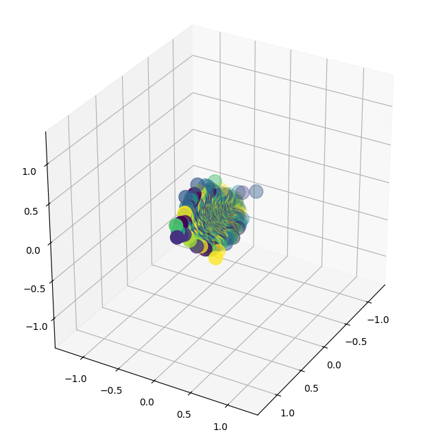
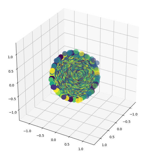
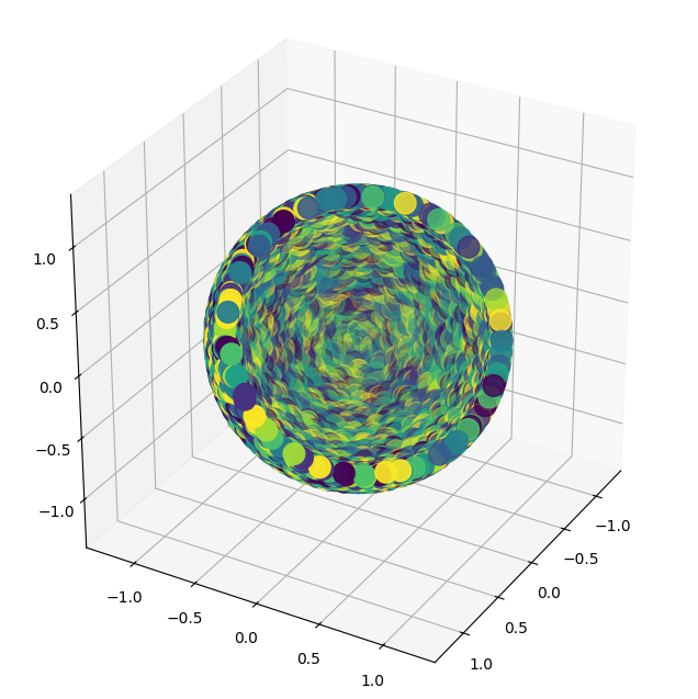
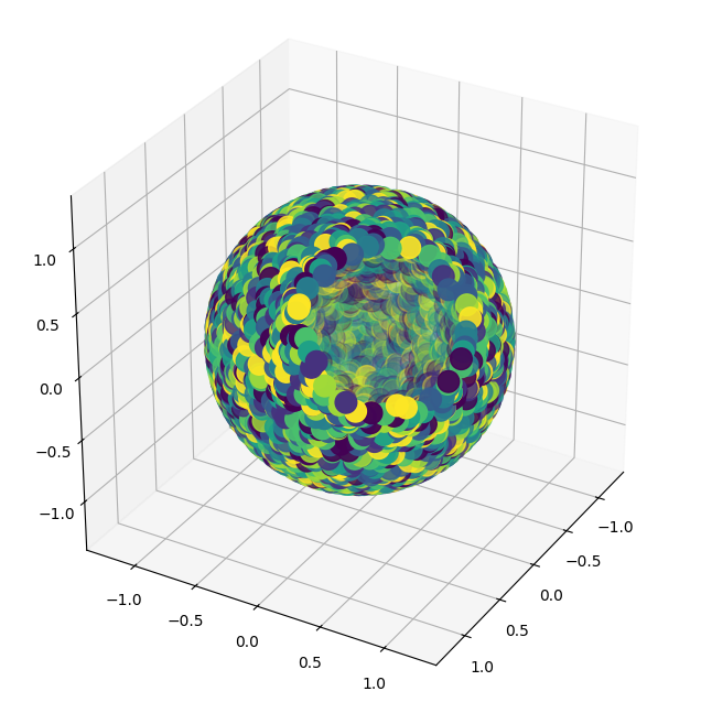
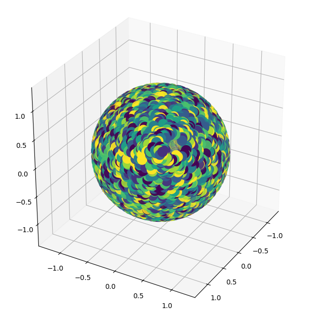
In this section, we provide additional experimental results to validate Theorem 4.5, showing that neural network optimization influences training dynamics. Even when starting with the same random initialization of the embedded distribution, the training dynamics with neural networks are guided toward stationary points where the clustering structure is imposed. In contrast, vanilla gradient descent without neural network optimization is independent of the data structure.
The comparison of optimization processes with and without neural network training in 2D and 3D is shown, with the data distribution presented in (a) and (l). A 4-layer fully connected neural network was used in this experiment, demonstrating that the same behavior is observed even with different neural network architectures. The color of each point corresponds to its respective cluster. Rows 2 and 5 illustrate optimization with neural network training, starting from a random initial embedding and progressively revealing the clustering structure over iterations. Rows 3 and 6 show the optimization process using vanilla gradient descent without neural network training. Over time, the distribution converges to a uniformly dispersed arrangement, disregarding the clustering structure of the input data.