Next-to-leading power jet functions in the small-mass limit in QED

Abstract

We investigate the factorization properties of the massive fermion form factor in QED, to next-to-leading power in the fermion mass, and up to two-loop order. For this purpose we define new jet functions that have multiple connections to the hard part as operator matrix elements, and compute them to second order in the coupling. We test our factorization formula using these new jet functions in a region-based analysis and find that factorization indeed holds. We address a number of subtle aspects such as rapidity regulators and external line corrections, and we find an interesting sequence of relations among the jet functions.

1 Introduction

Power corrections in scattering amplitudes have gained considerable attention in recent years (see e.g. refs. Low:1958sn ; Burnett:1967km ; DelDuca:1990gz ; Laenen:2008ux ; Laenen:2010uz ; Larkoski:2014bxa ; Bonocore:2014wua ; Ma:2014svb ; Kang:2014pya ; Bonocore:2015esa ; Bonocore:2016awd ; Moult:2016fqy ; Feige:2017zci ; Moult:2017rpl ; Moult:2017jsg ; Gervais:2017yxv ; DelDuca:2017twk ; Beneke:2017ztn ; Moult:2018jjd ; Beneke:2018rbh ; Beneke:2018gvs ; Ebert:2018lzn ; Bahjat-Abbas:2019fqa ; Moult:2019mog ; Beneke:2019kgv ; Beneke:2019mua ; Liu:2019oav ; Beneke:2019oqx ; vanBeekveld:2019prq ; vanBeekveld:2019cks ; Moult:2019uhz ; Liu:2020ydl ; Liu:2020eqe ; AH:2020iki ; AH:2020xll ; AH:2020qoa ; AH:2021kvg ; Beneke:2020ibj ; Laenen:2020nrt ; Liu:2020tzd ; vanBeekveld:2021hhv ; Broggio:2021fnr ; vanBeekveld:2021mxn ; Bonocore:2021qxh ; Engel:2021ccn ; Beneke:2022obx ; Bell:2022ott ; Liu:2022ajh ; Engel:2023ifn ; Engel:2023rxp ; Broggio:2023pbu ; vanBeekveld:2023gio ; vanBeekveld:2023liw ; Balsach:2023ema ; Beneke:2024cpq ; Beneke:2025ufd ). Besides their phenomenological relevance, the study of power corrections proves to be useful to deepen our understanding of gauge theory amplitudes. Scattering processes at hadron colliders often involve two or more widely separated scales, hence the corresponding amplitude can be expressed as a power expansion in the small ratio of such scales. In this work we focus in particular on the wide-angle scattering of $n$ energetic particles in quantum electrodynamics (QED), and consider them to have a small mass $m$ compared to the centre of mass energy $\sqrt{s}$, which represents a configuration to which most of the scattering processes occurring at high energy colliders can be traced back. The corresponding amplitude is expressed as a power expansion in $\lambda=m/\sqrt{s}\ll 1$, taking the form

$$\mathcal{M}=\mathcal{M}_{\textrm{LP}}+\mathcal{M}_{\rm\sqrt{N}LP}+\mathcal{M}_{\textrm{NLP}}+\mathcal{O}(\lambda^{3}),$$ (1)

where $\mathcal{M}_{\textrm{LP}}$ represents the leading power (LP) behaviour of this amplitude, while $\mathcal{M}_{\rm{\sqrt{N}LP}}$ and $\mathcal{M}_{\rm NLP}$ provide the first two power corrections in the expansion, of $\mathcal{O}(\lambda)$ and $\mathcal{O}(\lambda^{2})$ respectively.

Central to this paper is the expectation that, as shown by a power counting analysis in ref. Laenen:2020nrt , each term on the r.h.s. of eq. (1) factorizes into a product of hard, soft and jet functions. These represent respectively virtual hard modes, soft modes, and modes collinear to each of the $n$ external particles. Focusing in particular on the terms describing hard and collinear modes up to NLP, and soft modes at leading power, one has the following schematic factorization formula Laenen:2020nrt :

$$\mathcal{M}_{\mathrm{coll.}} =\left(\prod_{i=1}^{n}J_{f}^{i}\right)\otimes H_{f}\,S+\sum_{i=1}^{n}\bigg{(}\prod_{j\neq i}J_{f}^{j}\bigg{)}\Big{[}J^{i}_{f\gamma}\otimes H^{i}_{f\gamma}+J^{i}_{f\partial\gamma}\otimes H^{i}_{f\partial\gamma}\Big{]}\,S$$

$$\quad+\sum_{i=1}^{n}\bigg{(}\prod_{j\neq i}J_{f}^{j}\bigg{)}J^{i}_{f\gamma\gamma}\otimes H^{i}_{f\gamma\gamma}\,S+\sum_{i=1}^{n}\bigg{(}\prod_{j\neq i}J_{f}^{j}\bigg{)}J^{i}_{f\!f\!f}\otimes H^{i}_{f\!f\!f}\,S$$

$$\quad+\sum_{1\leq i\leq j\leq n}\bigg{(}\prod_{k\neq i,j}J_{f}^{k}\bigg{)}J^{i}_{f\gamma}J^{j}_{f\gamma}\otimes H^{ij}_{f\gamma,f\gamma}\,S+{\cal O}(\lambda^{3})\,,$$ (2)

where $H_{I}$ are process-dependent hard functions, $J_{I}$ represent universal jet functions, the soft function $S$ describes leading power virtual soft radiation. The symbol $\otimes$ denotes convolution.

The factorization at LP, given by the first term in eq. (1), has been known for a long time, see e.g. refs. Mueller:1979ih ; Collins:1980ih ; Collins:1981uk ; Sen:1981sd ; Collins:1989bt ; Dixon:2008gr . For massless particles it can be shown that the LP term in eq. (1) is in direct correspondence with the factorization structure of soft and collinear divergences Aybat:2006mz ; Gardi:2009qi ; Becher:2009qa , hence it provides the starting point for the resummation of large logarithms associated to the emission of soft and collinear radiation Magnea:1990zb ; Contopanagos:1996nh ; Kidonakis:1997gm ; Kidonakis:1998bk ; Magnea:2000ss . For massive particles, eq. (1) contains relevant information for the resummation of large logarithms of $m^{2}/s$ Catani:2000ef ; Penin:2005eh ; Penin:2005kf ; Mitov:2006xs ; Becher:2007cu ; Czakon:2007ej ; Czakon:2007wk ; Mitov:2009sv ; Becher:2009kw ; Banerjee:2020rww ; Wang:2023qbf ; Wang:2024pmv . The factorization of scattering amplitudes (or cross sections) into single-scale objects is at the basis of resummation, as it allows one to resum the large logarithms by means of renormalization group equations. In general, factorization theorems such as the one in eq. (1) have been derived directly in the original theory (QCD or, in the case considered here, QED) Sterman:1987aj ; Catani:1989ne ; Catani:1990rp ; Korchemsky:1993xv ; Korchemsky:1993uz , or within an approach based on the soft-collinear effective field theory (SCET), where soft and collinear modes are separated at the Lagrangian level Bauer:2000yr ; Bauer:2001yt ; Beneke:2002ph .

Much less is known concerning the factorization properties of the terms appearing beyond LP. Within SCET, factorization theorems for (massless) $n$-particle scattering amplitudes have been considered in the label formalism Larkoski:2014bxa ; Moult:2015aoa ; Kolodrubetz:2016uim ; Feige:2017zci and in the position-space formulation of SCET Beneke:2017ztn ; Beneke:2018rbh . Within the direct approach, factorization theorems have been discussed for $n$-particle amplitudes in the Yukawa theory Gervais:2017yxv and QED Laenen:2020nrt . An early discussion of factorization in Drell-Yan was presented in refs. Qiu:1990xxa ; Qiu:1990xy .

Although the power counting analysis in ref. Laenen:2020nrt has led to the factorization formula in eq. (1), the functions appearing in this equation have been defined so far only diagrammatically, i.e. by listing the Feynman diagrams expected to contribute to each function in QED. For the factorization theorem to be complete and serve as a basis for resummation, the jet functions in eq. (1) need to be properly defined in terms of matrix elements of time-ordered operators in QED, while the corresponding hard functions are matching coefficients. The aim of this paper is to fill this gap.

In this regard, let us recall that the factorization formula in eq. (1) is valid both for the case of massless and massive particles (with $m^{2}\ll s$). Indeed, while eq. (1) describes the factorization of an $n$-particle scattering amplitude, its relevance extends also to the case in which additional soft radiation is emitted. For this, as discussed in refs. Gervais:2017yxv ; Laenen:2020nrt , the jet functions are upgraded to radiative jet functions, and the emission of soft radiation from the hard functions is related to soft emissions from the other functions by Ward identities. Thus, the study we aim to conduct in this work is useful not only to complete and validate the factorization theorem in eq. (1), but is also preparatory to study the case of real radiation, which we leave for future analysis.

In order to validate the factorization theorem we should consider an amplitude sufficiently non-trivial that all functions appearing in eq. (1) contribute, yet simple enough that it can be calculated with standard methods known in literature. Moreover, functions such as $J_{f\gamma\gamma}$ and $J_{f\!f\!f}$ only contribute from two loops onwards, so that the validation of eq. (1) requires a complete two-loop calculation. The decay of an off-shell photon into a massive fermion-antifermion pair, usually described in literature in terms of massive fermion form factors, satisfies our requirements.

Much work has been dedicated to the perturbative calculation of the massive quark form factors. The two-loop result has been obtained in refs. Bernreuther:2004ih ; Gluza:2009yy (see also ref. Blumlein:2020jrf for a calculation of the corresponding contribution to the $e^{+}e^{-}\to\gamma^{*}/Z^{0*}$ cross section). In recent years a lot of effort has been devoted to the calculation of the three-loop correction Henn:2016kjz ; Henn:2016tyf ; Ablinger:2017hst ; Lee:2018nxa ; Lee:2018rgs ; Ablinger:2018yae ; Blumlein:2018tmz ; Blumlein:2019oas ; Fael:2022rgm ; Fael:2022miw ; Fael:2023zqr ; Blumlein:2023uuq , although no complete analytic result as yet exists. For our analysis we will need the two-loop region calculation obtained in ref. terHoeve:2023ehm , because a straightforward expansion of the results in refs. Bernreuther:2004ih ; Gluza:2009yy for $m^{2}\ll s$ is not enough to disentangle hard and collinear modes, which is needed to check the calculation of the jet functions in eq. (1).

Given these premises, our first task is to define and calculate the jet functions appearing in eq. (1). Then we will proceed to construct the corresponding photon-fermion-antifermion amplitude, and compare with the method of regions calculation. It may be worth mentioning here that the factorization formula in eq. (1) is given in terms of functions with open Lorentz and Dirac indices; no attempt is done to further project the jet functions onto a basis of scalar functions. This is not uncommon in case of factorization theorems beyond leading power, see e.g. ref. Beneke:2019oqx , as projecting to scalar functions would involve non-trivial projection operators, which we preferably avoid in order not to hide the relatively simple structure of eq. (1). In any case, the jet functions appearing in eq. (1) are universal objects, thus the results obtained in this paper are valid for any $n$-particle scattering amplitude.

The paper is structured as follows. In sec. 2 we describe the process of interest, set up our notation, recall factorization at leading power and then describe in detail the factorization structure of the terms contributing beyond leading power. In sec. 3 we give matrix element definitions for the new jet functions, and compute them at one loop, up to NLP. Sec. 4 then deals with factorization at two loops, which also includes the calculation of the relevant jet functions up to two loops. We compare our results to ref. terHoeve:2023ehm , region by region. We conclude and discuss our findings in sec. 5. App. A then discusses the interesting interplay between the $J_{f}$, $J_{f\gamma}$ and $J_{f\gamma\gamma}$ jet functions, where we demonstrate factorization for the double-collinear region at the integrand level. The derivation also shows that there is no double counting between the different (subleading) jet functions. In app. B we discuss the collinear-anticollinear factorization, and some of its subtle aspects. App. C reports the integral expressions for all the jet functions at two-loop order, while app. D discusses UV counterterms for the (factorized) amplitude, paying particular attention to mass renormalization.

2 Factorization in the small-mass limit

2.1 Fermion-antifermion amplitude in QED

Let us consider the QED process

$$\gamma^{*}(q)\to f(p_{1})+\bar{f}(p_{2}),$$ (3)

in which an off-shell photon with momentum $q$ produces a fermion-antifermion pair. Keeping cross sections in mind we also denote $q^{2}=s$. The fermions have mass $m$ so that $p_{1}^{2}=p_{2}^{2}=m^{2}$. In what follows we consider the corresponding unrenormalized, or bare, amplitude

$$V^{\mu}(p_{1},p_{2})=\bar{u}(p_{1})\,\Gamma^{\mu}(p_{1},p_{2})\,v(p_{2}),$$ (4)

where we make the important note that the amplitude also contains external line contributions, i.e. non-1PI diagrams. External line propagators are amputated according to the LSZ formalism. In the equation above we defined $\Gamma^{\mu}(p_{1},p_{2})$, which represents the amplitude with stripped-off spinors. At lowest order we have

$$\Gamma^{\mu(0)}(p_{1},p_{2})=i\,e\,e_{f}\,\gamma^{\mu},$$ (5)

where $e_{f}$ is the fermion electric charge in units of the positron charge $e>0$. In the small-mass limit $m\ll\sqrt{s}$, the amplitude $V^{\mu}(p_{1},p_{2})$ can be evaluated as a power expansion in the small parameter $\lambda\sim m/\sqrt{s}\ll 1$:

$$V^{\mu}\big{(}p_{1},p_{2}\big{)}=V_{\rm LP}^{\mu}\big{(}p_{1},p_{2}\big{)}+V_{\!\!\rm\sqrt{N}LP}^{\mu}\big{(}p_{1},p_{2}\big{)}+V_{\rm NLP}^{\mu}\big{(}p_{1},p_{2}\big{)}+{\cal O}\big{(}\lambda^{3}\big{)},$$ (6)

where $V_{\rm LP}^{\mu}$ is ${\cal O}(\lambda^{0})$, $V_{\!\!\rm\sqrt{N}LP}^{\mu}$ is ${\cal O}(\lambda)$, $V_{\rm NLP}^{\mu}$ is ${\cal O}(\lambda^{2})$, and so on. Central to our discussion is the expectation that each term on the r.h.s. of eq. (6) should factorize into hard, jet-like and soft structures, where the virtual momenta are respectively hard, i.e. of order $\sqrt{s}$, collinear to one of the two external fermions, or soft, i.e. of order $m^{2}$ Laenen:2020nrt ; terHoeve:2023ehm . Our goal is to verify that $V^{\mu}\big{(}p_{1},p_{2})$ factorizes according to eq. (1). To this end we will construct the factorized amplitude, and compare it with the recent calculation obtained by means of the method of regions terHoeve:2023ehm .

Let us start by setting the kinematic notation. We consider the centre-of-mass reference frame, where the outgoing momenta $p_{1}$ and $p_{2}$ read

$$p_{1}^{\mu}=\left(\sqrt{p^{2}+m^{2}},0,0,p\right),\qquad\quad p_{2}^{\mu}=\left(\sqrt{p^{2}+m^{2}},0,0,-p\right).$$ (7)

It proves useful to introduce two light-like vectors $n$ and $\bar{n}$, with $n^{2}=\bar{n}^{2}=0$ and $n\cdot\bar{n}=1$, with $p_{1}$ mostly along $n$ and $p_{2}$ mostly along $\bar{n}$, i.e.

$$p^{\mu}_{1}=p_{1}^{+}\,n^{\mu}+p_{1}^{-}\,\bar{n}^{\mu},\qquad\quad p^{\mu}_{2}=p_{2}^{+}\,n^{\mu}+p_{2}^{-}\,\bar{n}^{\mu}\,,$$ (8)

with

$$p_{1}^{+} =\bar{n}\cdot p_{1}=p_{2}^{-}=n\cdot p_{2}=\frac{1}{\sqrt{2}}\Big{(}\sqrt{p^{2}+m^{2}}+p\Big{)}\sim\sqrt{s},$$

$$p_{1}^{-} =n\cdot p_{1}=p_{2}^{+}=\bar{n}\cdot p_{2}=\frac{1}{\sqrt{2}}\Big{(}\sqrt{p^{2}+m^{2}}-p\Big{)}\sim\lambda^{2}\sqrt{s}.$$ (9)

The mass-shell condition implies

$$p_{i}^{2}=2p_{i}^{+}p_{i}^{-}=m^{2}\implies p_{1}^{-}=\frac{m^{2}}{2p_{1}^{+}},\quad p_{2}^{+}=\frac{m^{2}}{2p_{2}^{-}}.$$ (10)

We then have

$$s=(p_{1}+p_{2})^{2}=2m^{2}+2p_{1}^{+}p_{2}^{-}+2p_{1}^{-}p_{2}^{+}=\hat{s}\left(1+\frac{2m^{2}}{\hat{s}}+\frac{m^{4}}{\hat{s}^{2}}\right),$$ (11)

where we defined the $\mathcal{O}(\lambda^{0})$ variable $\hat{s}\equiv 2p_{1}^{+}p_{2}^{-}$. In what follows we will refer to the direction identified by the vector $n$ as collinear ($c$), while the direction identified by $\bar{n}$ will be labelled as anticollinear ($\bar{c}$). Where needed we will indicate the large components of $p_{1}$ and $p_{2}$ by

$$\hat{p}_{1}^{\mu} =p_{1}^{+}\,n^{\mu},\qquad\qquad\qquad\hat{p}_{2}^{\mu}=p_{2}^{-}\,\bar{n}^{\mu},$$ (12)

while the corresponding small components will be indicated by

$$\tilde{p}_{1}^{\mu} =p_{1}^{-}\,\bar{n}^{\mu},\qquad\qquad\qquad\tilde{p}_{2}^{\mu}=p_{2}^{+}\,n^{\mu}.$$ (13)

A generic momentum is decomposed along $n$, $\bar{n}$ as follows:

$$k^{\mu}=k^{+}\,n^{\mu}+k^{-}\,\bar{n}^{\mu}+k_{\perp}^{\mu},\qquad\qquad\quad k^{\mu}=(k^{+},k^{-},k_{\perp}),$$ (14)

where $k^{+}=\bar{n}\cdot k$, $k^{-}=n\cdot k$. This notation can be used to express scaling relations. For instance, $p^{\mu}_{1}=(p_{1}^{+},p_{1}^{-},p_{1\perp})\sim\sqrt{s}(\lambda^{0},\lambda^{2},0)$, $p^{\mu}_{2}=(p_{2}^{+},p_{2}^{-},p_{2\perp})\sim\sqrt{s}(\lambda^{2},\lambda^{0},0)$. In general, virtual momenta leading to non-scaleless contributions have the scaling properties

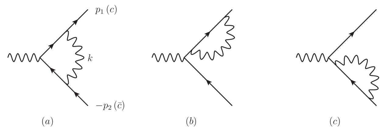
Figure 1: One-loop diagrams contributing to the $\gamma\to f\bar{f}$ amplitude, according to the conventions discussed in the main text. The momenta $p_{1}$ and $p_{2}$ are outgoing.

hard ($$h k\sim\sqrt{s}\,(\lambda^{0},\lambda^{0},\lambda^{0})\,,$$):

collinear ($$c k\sim\sqrt{s}\,(\lambda^{0},\lambda^{2},\lambda^{1})\,,$$): (15)

anticollinear ($$\bar{c} k\sim\sqrt{s}\,(\lambda^{2},\lambda^{0},\lambda^{1})\,.$$):

With these conventions we are almost ready to discuss the factorization of the amplitude for the case $m\ll\sqrt{s}$. Before proceeding we highlight the fact that, as stated below eq. (4), we are considering here the full amplitude and therefore include self-energy contributions on the external legs, order by order in perturbation theory. As will become clear in sec. 3, this is because the jet functions defined within the factorization theorem in eq. (1) naturally include such contributions. Therefore, we need to include the self-energy corrections in the region calculation in QED as well, for a proper comparison. Thus the one-loop amplitude $V^{\mu(1)}\big{(}p_{1},p_{2}\big{)}$ will receive contributions from all diagrams listed in fig. 1. The inclusion of self-energy corrections modifies the equation of motion and the mass-shell condition, and corrections can be included order by order in perturbation theory. The self-energy contribution is usually taken into account by means of a Dyson sum:

$$\frac{i}{\not{p}-m}\bigg{\{}1+\Big{[}i\,\Sigma(p)\Big{]}\frac{i}{\not{p}-m}+\mathcal{O}(\alpha^{2})\bigg{\}}=\frac{i}{\not{p}-m+\Sigma(p)}.$$ (16)

Here $\Sigma(p)$ has the general form

$$\Sigma(p)=A(p^{2})\,\not{p}+B(p^{2})\,m,$$ (17)

such that the propagator can be rewritten as

$$\frac{iR}{\not{p}-m_{p}},\qquad R^{-1}=1+A(m_{p}^{2})+\mathcal{O}(p^{2}-m_{p}^{2}),\qquad m_{p}=m\left(\frac{1-B(m_{p}^{2})}{1+A(m_{p}^{2})}\right),$$ (18)

where $m_{p}$ represents the unrenormalized pole mass. At one loop one has Honemann:2018mrb

$$A(m^{2}) = \frac{\alpha\,e_{f}^{2}}{4\pi}\left(\frac{\bar{\mu}^{2}}{m^{2}}\right)^{\epsilon}\left[\frac{1}{\epsilon}+2+\bigg{(}4+\frac{\zeta_{2}}{2}\bigg{)}\epsilon+\bigg{(}8+\zeta_{2}-\frac{\zeta_{3}}{3}\bigg{)}\epsilon^{2}+\mathcal{O}(\epsilon^{3})\right]+{\cal O}(\alpha^{2}),$$

$$B(m^{2}) = \frac{\alpha\,e_{f}^{2}}{4\pi}\left(\frac{\bar{\mu}^{2}}{m^{2}}\right)^{\epsilon}\left[-\frac{4}{\epsilon}-6-(12+2\zeta_{2})\epsilon-\bigg{(}24+3\zeta_{2}-\frac{4\zeta_{3}}{3}\bigg{)}\epsilon^{2}+\mathcal{O}(\epsilon^{3})\right]+{\cal O}(\alpha^{2}),$$ (19)

where $\alpha\equiv\alpha_{\rm EM}=e^{2}/4\pi$. Here we evaluated $A$ and $B$ in $m^{2}$, and not in $m_{p}^{2}$, since differences are of higher order in $\alpha$. As a consequence the equation of motion are modified as

$$\bar{u}(p_{1})\not{p}_{1} = \bar{u}(p_{1})\,m\Big{[}1-A(m^{2})-B(m^{2})+\mathcal{O}(\alpha^{2})\Big{]},$$

$$\not{p}_{2}v(p_{2}) = -m\Big{[}1-A(m^{2})-B(m^{2})+\mathcal{O}(\alpha^{2})\Big{]}\,v(p_{2}),$$ (20)

or upon expanding in powers of $\lambda$:

$$\bar{u}(p_{1})\,\not{n} = \bar{u}(p_{1})\frac{1}{p_{1}^{+}}\bigg{\{}m\Big{[}1-A(m^{2})-B(m^{2})+\mathcal{O}(\alpha^{2})\Big{]}-p_{1}^{-}\,\not{\bar{n}}\bigg{\}},$$

$$\not{\bar{n}}\,v(p_{2}) = -\bigg{\{}m\Big{[}1-A(m^{2})-B(m^{2})+\mathcal{O}(\alpha^{2})\Big{]}+p_{2}^{+}\,\not{n}\bigg{\}}\frac{1}{p_{2}^{-}}v(p_{2}).$$ (21)

Similarly, beyond tree level the mass-shell condition in eq. (10) is modified accordingly. Up to one loop one has

$$p_{i}^{2}=m^{2}\Big{[}1-2A(m^{2})-2B(m^{2})+\mathcal{O}(\alpha^{2})\Big{]}.$$ (22)

We are now ready to discuss the factorization of the power expansion of $V^{\mu}(p_{1},p_{2})$ for $m\ll\sqrt{s}$.

2.2 Factorization at LP

In order to set up the factorization formula up to NLP, we start with the leading power term. The case of massless fermions has been discussed at length in ref. Dixon:2008gr . The factorization formula for the massive case is formally equivalent. For an outgoing fermion-antifermion pair it reads

$$V_{\rm LP}^{\mu}(p_{1},p_{2},\mu)=H_{f,\bar{f}}^{\mu}(\hat{p}_{1},\hat{p}_{2},\mu)\,\frac{J_{f}(p_{1},\bar{n},\mu)}{{\cal J}_{f}(n,\bar{n},\mu)}\,\frac{J_{\bar{f}}(p_{2},n,\mu)}{{\cal J}_{\bar{f}}(\bar{n},n,\mu)}\,S_{f,\bar{f}}(n\cdot\bar{n},\mu),$$ (23)

where $\mu$ represents the factorization scale. In what follows we will keep the dependence on $\mu$ implicit, unless needed. The convention for now and what follows is that $f$ is for the fermion line (in the $c$-collinear direction) with outgoing momentum $p_{1}$, and the $\bar{f}$ is for the antifermion line (in the $\bar{c}$-collinear, i.e. anticollinear, direction) with outgoing momentum $p_{2}$. In eq. (23) the hard function $H_{f,\bar{f}}^{\mu}(\hat{p}_{1},\hat{p}_{2})$ represents the virtual hard modes, thus it depends on the large momentum components $\hat{p}_{1}^{\mu}$, $\hat{p}_{2}^{\mu}$ defined in eq. (12). Next, the jet functions $J_{f}(p_{1},\bar{n})$ and $J_{\bar{f}}(p_{2},n)$ reproduce virtual collinear and anticollinear modes respectively, and are defined in terms of matrix elements of (implicitly) time-ordered operators

$$J_{f}(p_{1},n_{1},\mu)=\big{\langle}p_{1}\big{|}\bar{\psi}(0)\,\Phi_{n_{1}}(0,\infty)\big{|}0\big{\rangle},$$ (24)

and

$$J_{\bar{f}}(p_{2},n_{2},\mu)=\big{\langle}p_{2}\big{|}\Phi_{n_{2}}(\infty,0)\,\psi(0)\big{|}0\big{\rangle},$$ (25)

where $n_{1}$ and $n_{2}$ represent gauge-link vectors associated to the definition of the Wilson line

$$\Phi_{n}(y,x)={\cal P}\exp[i\,e\,e_{f}\int_{x}^{y}ds\,n\cdot A(sn)\bigg{]}.$$ (26)

The direction of the Wilson line is largely arbitrary, but given that their function is to mimic the coupling of photons collinear to the outgoing parton (say, the fermion) to the opposite moving hard parton (i.e., the antifermion), we choose $n_{1}=\bar{n}$, $n_{2}=n$, as indicated in eq. (23). Lastly, eq. (23) contains the soft function $S_{f,\bar{f}}(n\cdot\bar{n})$, as well as the eikonal approximation of the two jet functions, all defined in terms of the vacuum expectation value of Wilson lines. One has

$$S_{f,\bar{f}}(\hat{\beta}_{1}\cdot\hat{\beta}_{2},\mu)=\big{\langle}0\big{|}\Phi_{\hat{\beta}_{1}}(\infty,0)\,\Phi_{\hat{\beta}_{2}}(0,\infty)\big{|}0\big{\rangle}$$ (27)

for the soft function, and

$${\cal J}_{f}(\hat{\beta}_{1},n_{1},\mu) = \big{\langle}0\big{|}\Phi_{\hat{\beta}_{1}}(\infty,0)\,\Phi_{n_{1}}(0,\infty)\big{|}0\big{\rangle},$$

$${\cal J}_{\bar{f}}(\hat{\beta}_{2},n_{2},\mu) = \big{\langle}0\big{|}\Phi_{n_{2}}(\infty,0)\,\Phi_{\hat{\beta}_{2}}(0,\infty)\big{|}0\big{\rangle}$$ (28)

for the two eikonal jet functions. Note that these eikonal jet functions prevent overcounting between the jet function and the soft function. Observe also that, for simplicity, in eqs. (27) and (2.2) we approximate the velocities of the fermion and antifermion pair, $\beta_{1}$ and $\beta_{2}$, with the directions of large momentum flow, i.e. $\beta_{1}\sim\hat{\beta}_{1}=n$, $\beta_{2}\sim\hat{\beta}_{2}=\bar{n}$, as already indicated implicitly in eq. (23).

The most important aspect to underline concerning eq. (23) is that it describes the factorization of the amplitude after soft and collinear singularities have been moved from the hard function to the jet and soft functions. Let us clarify this relevant point. Loop corrections to the amplitude $V^{\mu}\big{(}p_{1},p_{2})$ in general contain soft and collinear divergences in case of massless fermions, and just soft divergences in case of massive fermions, as considered here. (There are ultraviolet divergences as well; these can be removed by standard UV renormalization. We discuss these in app. D.) Calculating $V^{\mu}\big{(}p_{1},p_{2})$ by means of the method of regions generates spurious singularities within each region, such that the original singularities are reproduced only after the sum of all regions has been considered. In the case at hand, we know terHoeve:2023ehm that the massive form factor receives contributions from the hard, collinear and anticollinear regions. The hard region develops soft and (spurious) collinear singularities, while the collinear and anticollinear regions develop soft and (spurious) ultraviolet singularities, such that in the sum collinear and ultraviolet singularities cancel, leaving the soft singularities. In general, it is preferred to define the functions appearing in the factorization eq. (23) such that only the “true” singularities appear explicitly: in other words, one wants to define a hard function free of collinear and soft singularities, and associate collinear divergences to the jet functions (in case of massless particles) and soft divergences to the soft function. For the massless case, this is discussed at length in ref. Dixon:2008gr , to which we refer for further details. Focusing on the problem at hand, both the bare soft function and eikonal jets are scaleless. The standard interpretation of scaleless regions in dimensional regularization is that one has infrared and ultraviolet divergences cancelling each other, such that $1/\epsilon_{\rm IR}-1/\epsilon_{\rm UV}=0$. Thus, in order to achieve the factorization structure in eq. (23), one splits this singularity structure: the ultraviolet pole moves into the hard function. The soft function then contains the leftover infrared divergence, and it becomes a pure counterterm. In the problem at hand, given that only the hard, collinear and anticollinear regions are not scaleless, both the soft function $S_{f,\bar{f}}(\beta_{1}\cdot\beta_{2})$ and the eikonal jets ${\cal J}_{f}(\beta_{1})$, ${\cal J}_{\bar{f}}(\beta_{2})$ in eq. (23) contribute as pure counterterms.

However, in our approach we do not redistribute the poles over the various functions, but rather compute them at face value. Thus we aim to check that the various jet functions that appear up to subleading power are able to reproduce the contribution given by the collinear and anticollinear regions. Hence, we aim to reproduce the factorization theorem in eq. (23) (and its generalization at subleading power, to be discussed) in its “bare” form, i.e., before soft (and collinear) singularities are reshuffled into pure-counterterm soft and eikonal jet functions. For the leading power contribution this implies that we aim to prove

$$V_{\rm LP}^{\mu}(p_{1},p_{2},\mu)=H_{f,\bar{f}}^{\mu,b}(\hat{p}_{1},\hat{p}_{2},\mu)\,J_{f}^{b}(\hat{p}_{1},\bar{n},\mu)\,J_{\bar{f}}^{b}(\hat{p}_{2},n,\mu),$$ (29)

where the index $b$, for “bare”, means that no reshuffling of soft and collinear singularities has been considered. In what follows we will always intend a factorization theorem as written in eq. (29), and drop the index $b$ for simplicity.

2.3 Factorization at NLP

We are now ready to specialize the factorization formula in eq. (1) to the case of a fermion-antifermion pair. In order to keep equations short, we assign a name to the various terms in eq. (1). The factorization formula then becomes a sum over factorized terms:

$$V^{\mu}\big{(}p_{1},p_{2}) = V_{f,\bar{f}}^{\mu}(p_{1},p_{2})+V_{f\gamma,\bar{f}}^{\mu}(p_{1},p_{2})+V_{f\partial\gamma,\bar{f}}^{\mu}(p_{1},p_{2})+V_{f,\bar{f}\gamma}^{\mu}(p_{1},p_{2})+V_{f,\bar{f}\partial\gamma}^{\mu}(p_{1},p_{2})$$ (30)

$$+\,V_{f\gamma\gamma,\bar{f}}^{\mu}(p_{1},p_{2})+V_{f,\bar{f}\gamma\gamma}^{\mu}(p_{1},p_{2})+V_{f\!f\!\bar{f},\bar{f}}^{\mu}(p_{1},p_{2})+V_{f,\bar{f}\!f\!\bar{f}}^{\mu}(p_{1},p_{2})$$

$$+\,V_{f\gamma,\bar{f}\gamma}^{\mu}(p_{1},p_{2})+{\cal O}\big{(}\lambda^{3}\big{)},$$

which we discuss one by one in what follows. First of all we have

$$V_{f,\bar{f}}^{\mu}(p_{1},p_{2})=J_{f}(p_{1},\bar{n})\,H_{f,\bar{f}}^{\mu}(p_{1};p_{2})\,J_{\bar{f}}(p_{2},n),$$ (31)

which represents a configuration involving a fermion along the collinear direction and an antifermion along the anticollinear direction, as depicted in fig. 2 (a). All additional virtual radiation is either hard, factorized into the hard function, or (anti)collinear along the two directions ($\bar{n}$) $n$, and factorized into the two jet functions. This term starts at ${\cal O}(\lambda^{0})$ and it is obviously a generalization of the leading power term in eq. (29). In this regard, let us highlight that the hard and jet functions in the LP factorization formula depend on the leading momentum components $\hat{p}_{i}$. In contrast, in order to reach ${\cal O}(\lambda^{2})$ (i.e., NLP) accuracy in eq. (31), we start by retaining the dependence on the full momenta $p_{i}$, and expand the jet and hard functions in eq. (31) into the mass $m\sim{\cal O}(\lambda)$ and the small momentum components $\tilde{p}_{i}\sim{\cal O}(\lambda^{2})$. Indeed, exploiting the mass-shell condition in eqs. (10) and (22), we can express the small momentum component as a function of the mass. Each function in eq. (31) becomes a power series in $m$. Combining the large components $p_{1}^{+}$, $p_{2}^{-}$ into $\hat{s}$ according to eq. (11) we have

$$H_{f,\bar{f}}^{\mu}(p_{1};p_{2})=H_{f,\bar{f}}^{\mu}(\hat{s},m) = \bigg{(}1+m\frac{\partial}{\partial m}+\frac{m^{2}}{2}\frac{\partial^{2}}{\partial m^{2}}\bigg{)}H_{f,\bar{f}}^{\mu}(\hat{s},m)\Big{|}_{m=0}+{\cal O}(\lambda^{3})$$ (32)

$$= H_{f,\bar{f}}^{\mu}(\hat{s})\big{|}_{\rm LP}+m\,H_{f,\bar{f}}^{\mu}(\hat{s})\big{|}_{\rm\sqrt{N}LP}+\frac{m^{2}}{2}\,H_{f,\bar{f}}^{\mu}(\hat{s})\big{|}_{\rm NLP}+{\cal O}(\lambda^{3}),$$

and

$$J_{f}(p_{1},\bar{n})=J_{f}(m,\bar{n})\big{|}_{\rm LP}+\frac{m}{p_{1}^{+}}J_{f}(m,\bar{n})\big{|}_{\rm\sqrt{N}LP}+\frac{m^{2}}{(p_{1}^{+})^{2}}J_{f}(m,\bar{n})\big{|}_{\rm NLP}+{\cal O}(\lambda^{3}),$$ (33)

with an equivalent expansion for $J_{\bar{f}}(p_{2},n)$. The series in eqs. (32) and (33) can then be inserted in eq. (31) to get a systematic expansion of $V_{f,\bar{f}}^{\mu}$.

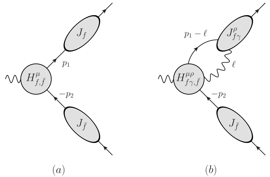
Figure 2: Diagrammatic representation of $V_{f,\bar{f}}^{\mu}$ (a) and $V_{f\gamma,\bar{f}}^{\mu}$ (b), defined respectively in eqs. (31) and (35).

The next terms in eq. (30) are given respectively by $V_{f\gamma,\bar{f}}^{\mu}$ and $V_{f\partial\gamma,\bar{f}}^{\mu}$. They describe a configuration involving a fermion and a transverse photon along the collinear direction, and an antifermion along the anticollinear direction, as represented in fig. 2 (b). Similarly, the terms $V_{f,\bar{f}\gamma}^{\mu}$ and $V_{f,\bar{f}\partial\gamma}^{\mu}$ involve a fermion along the collinear direction, and an antifermion plus a transverse photon along the anticollinear direction. They can be obtained by symmetry from $V_{f\gamma,\bar{f}}^{\mu}$ and $V_{f\partial\gamma,\bar{f}}^{\mu}$, by exchanging $p_{1}\leftrightarrow-p_{2}$, thus we will not discuss them further.

In order to write down the explicit form of $V_{f\gamma,\bar{f}}^{\mu}$ and $V_{f\partial\gamma,\bar{f}}^{\mu}$, let us label the photon momentum by $\ell$, as indicated in fig. 2 (b). Consequently, the hard function for this process, $H_{f\gamma,\bar{f}}^{\mu\rho}$, involves a collinear fermion and a photon, respectively with momenta $p_{1}-\ell$ and $\ell$, with $\ell=(\ell^{+},\ell^{-},\ell_{\perp})\sim\sqrt{s}\,(\lambda^{0},\lambda^{2},\lambda^{1})$. As argued in ref. Laenen:2020nrt , a consistent factorization order by order in the power expansion requires the hard function to depend only on the large momentum component $\hat{\ell}=\ell^{+}n$ (as well as $\hat{p}_{1}$). This is achieved by expanding $H_{f\gamma,\bar{f}}^{\mu}$ in the small components of $\ell$. Anticipating that the jet function $J^{\rho}_{f\gamma}$ starts at ${\cal O}(\lambda)$, we need to expand the hard function up to ${\cal O}(\lambda)$ as well. We thus have

$$H_{f\gamma,\bar{f}}^{\mu\rho}(p_{1}-\ell,\ell;p_{2}) = \bigg{(}1+\ell^{\sigma}_{\perp}\frac{\partial}{\partial\ell^{\sigma}_{\perp}}\bigg{)}H_{f\gamma,\bar{f}}^{\mu\rho}(p_{1}-\ell,\ell;p_{2})\Big{|}_{\ell_{\perp}=0}+{\cal O}(\lambda^{2})$$ (34)

$$= H_{f\gamma,\bar{f}}^{\mu\rho}(p_{1}-\hat{\ell},\hat{\ell};p_{2})+\ell_{\perp\sigma}\,H_{f\partial\gamma,\bar{f}}^{\mu\rho\sigma}(\hat{p}_{1}-\hat{\ell},\hat{\ell};\hat{p}_{2})+{\cal O}(\lambda^{2}),$$

where in the second line we have implicitly defined $H_{f\partial\gamma,\bar{f}}^{\mu\rho\sigma}$. Given eq. (34), $V_{f\gamma,\bar{f}}^{\mu}$ and $V_{f\partial\gamma,\bar{f}}^{\mu}$ still involve a convolution over the large momentum component $l^{+}$. We have respectively

$$V_{f\gamma,\bar{f}}^{\mu}(p_{1},p_{2})=\int_{0}^{p_{1}^{+}}d\ell^{+}\,J_{f\gamma\,\rho}(p_{1}-\hat{\ell},\hat{\ell},\bar{n})\,H_{f\gamma,\bar{f}}^{\mu\rho}(p_{1}-\hat{\ell},\hat{\ell};p_{2})\,J_{\bar{f}}(p_{2},n),$$ (35)

and

$$V_{f\partial\gamma,\bar{f}}^{\mu}(p_{1},p_{2})=\int_{0}^{p_{1}^{+}}d\ell^{+}\,J_{f\partial\gamma\,\rho\sigma}(\hat{p}_{1}-\hat{\ell},\hat{\ell},\bar{n})\,H_{f\partial\gamma,\bar{f}}^{\mu\rho\sigma}(\hat{p}_{1}-\hat{\ell},\hat{\ell};\hat{p}_{2})\,J_{\bar{f}}(\hat{p}_{2},n).$$ (36)

A few comments are in order. First, $V_{f\gamma,\bar{f}}^{\mu}$ starts at ${\cal O}(\lambda)$. Thus, the jet and hard functions still need to be expanded in powers of $m$, for a consistent expansion up to ${\cal O}(\lambda^{2})$. Similarly to the series definitions in eqs. (32) and (33), we have

$$H_{f\gamma,\bar{f}}^{\mu\rho}(p_{1}-\hat{\ell},\hat{\ell};p_{2}) = \bigg{(}1+m\frac{\partial}{\partial m}\bigg{)}H_{f\gamma,\bar{f}}^{\mu\rho}(p_{1}-\hat{\ell},\hat{\ell};p_{2})\bigg{|}_{m=0}+{\cal O}(\lambda^{2})$$ (37)

$$= H_{f\gamma,\bar{f}}^{\mu\rho}(\hat{p}_{1}-\hat{\ell},\hat{\ell};\hat{p}_{2})\big{|}_{\rm LP}+m\,H_{f\gamma,\bar{f}}^{\mu\rho}(\hat{p}_{1}-\hat{\ell},\hat{\ell};\hat{p}_{2})\big{|}_{\rm\sqrt{N}LP}+{\cal O}(\lambda^{2}),$$

and

$$J^{\rho}_{f\gamma}(p_{1}-\hat{\ell},\hat{\ell},\bar{n})=J^{\rho}_{f\gamma}(\hat{p}_{1}-\hat{\ell},\hat{\ell},\bar{n})\big{|}_{\rm\sqrt{N}LP}+\frac{m}{p_{1}^{+}}J^{\rho}_{f\gamma}(\hat{p}_{1}-\hat{\ell},\hat{\ell},\bar{n})\big{|}_{\rm NLP}+{\cal O}(\lambda^{3}).$$ (38)

The series in eqs. (37) and (38) can be inserted in eq. (35) to get a systematic expansion of $V_{f\gamma,\bar{f}}^{\mu}$. Concerning eq. (36), we point out that we have absorbed the factor $\ell^{\sigma}_{\perp}$ in eq. (34) into the definition of $J^{\rho\sigma}_{f\partial\gamma}$. Schematically we may write

$$J^{\rho\sigma}_{f\partial\gamma}(\hat{p}_{1}-\hat{\ell},\hat{\ell},\bar{n})=J^{\rho}_{f\gamma}(\hat{p}_{1}-\hat{\ell},\hat{\ell},\bar{n})\,\ell^{\sigma}_{\perp},$$ (39)

where we stress that $J^{\rho}_{f\gamma}$ involves an integration over $\ell_{\perp}$, thus the explicit factor of $\ell^{\sigma}_{\perp}$ in eq. (39) is integrated over as well. In sec. 3.2 we will see that $J^{\rho\sigma}_{f\partial\gamma}$ can be rigorously defined in terms of an operator matrix element. $V_{f\partial\gamma,\bar{f}}^{\mu}$ starts at ${\cal O}(\lambda^{2})$, so there is no need to further expand in powers of $m$, as in eqs. (37) and (38). Thus, the functions $J_{f\partial\gamma}^{\rho\sigma}$ and $H_{f\partial\gamma,\bar{f}}^{\mu\rho\sigma}$ are taken at leading order in the power expansion, and depend only on the leading momentum components, as indicated by the argument of the functions in eq. (36).

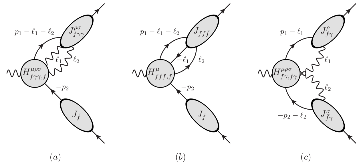
Figure 3: Diagrammatic representation of $V_{f\gamma\gamma,\bar{f}}^{\mu}$ (a), $V_{f\!f\!\bar{f},\bar{f}}^{\mu}$ (b) and $V_{f\gamma,\bar{f}\gamma}^{\mu}$ (c), defined respectively in eqs. (40), (41) and (42).

The remaining terms in eq. (30) are $V_{f\gamma\gamma,\bar{f}}^{\mu}$, $V_{f\!f\!\bar{f},\bar{f}}^{\mu}$ and $V_{f\gamma,\bar{f}\gamma}^{\mu}$, as well as the corresponding $p_{1}\leftrightarrow-p_{2}$ symmetric terms $V_{f,\bar{f}\gamma\gamma}^{\mu}$ and $V_{f,\bar{f}\!\bar{f}\!f}^{\mu}$. All these terms start at ${\cal O}(\lambda^{2})$, therefore we can consistently drop all dependence on $\ell_{1\perp}$, $\ell_{2\perp}$ and all other small momentum components. The terms $V_{f\gamma\gamma,\bar{f}}^{\mu}$ and $V_{f\!f\!\bar{f},\bar{f}}^{\mu}$ involve a configuration respectively with a fermion and two (transverse) photons or a fermion and a fermion-antifermion pair along the collinear direction, and an antifermion along the anticollinear direction, as represented in fig. 3 (a) and (b). They involve a convolution over the large momentum components $\hat{\ell}_{1}$, $\hat{\ell}_{2}$ as follows:

$$V_{f\gamma\gamma,\bar{f}}^{\mu}\big{(}p_{1},p_{2})=\int_{0}^{p_{1}^{+}}d\ell_{1}^{+}\,d\ell_{2}^{+}\,J_{f\gamma\gamma\,\rho\sigma}(\hat{p}_{1}-\hat{\ell}_{1}-\hat{\ell}_{2},\hat{\ell}_{1},\hat{\ell}_{2},\bar{n})\,H_{f\gamma\gamma,\bar{f}}^{\mu\rho\sigma}(\hat{p}_{1}-\hat{\ell}_{1}-\hat{\ell}_{2},\hat{\ell}_{1},\hat{\ell}_{2};\hat{p}_{2})\,J_{\bar{f}}(\hat{p}_{2},n),$$ (40)

and

$$V_{f\!f\!\bar{f},\bar{f}}^{\mu}\big{(}p_{1},p_{2})=\int_{0}^{p_{1}^{+}}d\ell_{1}^{+}\,d\ell_{2}^{+}\,J_{f\!f\!\bar{f}}(\hat{p}_{1}-\hat{\ell}_{1}-\hat{\ell}_{2},\hat{\ell}_{1},\hat{\ell}_{2},\bar{n})\,H^{\mu}_{f\!f\!\bar{f},\bar{f}}(\hat{p}_{1}-\hat{\ell}_{1}-\hat{\ell}_{2},\hat{\ell}_{1},\hat{\ell}_{2};\hat{p}_{2})\,J_{\bar{f}}(\hat{p}_{2},n).$$ (41)

Here we use simplified notation. In sec. 4.3.4 we distinguish two contributions that differ by charge flow. The last term, i.e. $V_{f\gamma,\bar{f}\gamma}^{\mu}$, involves a configuration with a collinear fermion and photon, as well as an anticollinear antifermion and photon, as depicted in fig. 3 (c). As such it also involves two convolutions, over $\ell_{1}^{+}$ and $\ell_{2}^{-}$. It reads

$$V_{f\gamma,\bar{f}\gamma}^{\mu}\big{(}p_{1},p_{2}) = \int_{0}^{p_{1}^{+}}d\ell_{1}^{+}\int_{0}^{p_{2}^{-}}d\ell_{2}^{-}\,J_{f\gamma\,\rho}(\hat{p}_{1}-\hat{\ell}_{1},\hat{\ell}_{1},\bar{n})$$ (42)

$$\hskip 28.45274pt\times\,H_{f\gamma,\bar{f}\gamma}^{\mu\rho\sigma}(\hat{p}_{1}-\hat{\ell}_{1},\hat{\ell}_{1},-\hat{p}_{2}-\hat{\ell}_{2},\hat{\ell}_{2})\,J_{\bar{f}\gamma\,\sigma}(-\hat{p}_{2}-\hat{\ell}_{2},\hat{\ell}_{2},n).$$

With these definitions at hand, each term in eq. (30) has been properly defined in terms of convolutions between hard and jet functions. In this regard, let us notice that, although we defined the convolutions in eqs. (35) and (36) in terms of the large photon momentum component $\ell^{+}$, and the convolutions in eqs. (40), (41) and (42) in terms of the large components $\ell_{1}^{+}$ and $\ell_{2}^{+}$ (or $\ell_{2}^{-}$ for the case in eq. (42)), in practice it will be more convenient to express the convolutions in terms of dimensionless momentum fractions, for instance

$$V_{f\gamma,\bar{f}}^{\mu}(p_{1},p_{2})=p_{1}^{+}\int_{0}^{1}dx\,J_{f\gamma\,\rho}(p_{1}-\hat{\ell},\hat{\ell},\bar{n})\,H_{f\gamma,\bar{f}}^{\mu\rho}(p_{1}-\hat{\ell},\hat{\ell};p_{2})\,J_{\bar{f}}(p_{2},n),$$ (43)

with $x\equiv\ell^{+}/p_{1}^{+}$.

Our next goal is to show that each jet function can be defined in terms of an operator matrix element in QED. In this context, each hard function can be considered as the corresponding short-distance (Wilson) coefficient, which can be obtained by matching with the full amplitude in QED. We devote secs. 3 and 4 to the jet function definitions in terms of operator matrix elements, and their calculation in perturbation theory up to the perturbative order required to reproduce the full amplitude up to ${\cal O}(\alpha^{2})$.

2.4 Form factors in the limit $m^{2}\ll s$

In order to check that the factorized amplitude in eq. (30) correctly reproduces the QED amplitude in the limit $m^{2}\ll s$, we compare our calculation in terms of hard and jet functions with the massive form factors calculation obtained in ref. terHoeve:2023ehm by means of the method of regions. To this end, let us briefly recall that the $\gamma\to f\bar{f}$ amplitude can be expressed in terms of two form factors $F_{1}$ and $F_{2}$ such that

$$\Gamma^{\mu}(p_{1},p_{2})=i\,e\,e_{f}\bigg{[}F_{1}(s,m)\gamma^{\mu}+\frac{1}{2m}F_{2}(s,m)\,i\,\sigma^{\mu\nu}(p_{1}+p_{2})_{\nu}\bigg{]},$$ (44)

where $\sigma^{\mu\nu}=\frac{i}{2}[\gamma^{\mu},\gamma^{\nu}]$, and the electric charge is consistent with eq. (5). In the rest of the paper we will take $e_{f}=-1$, except those equations where the factor $e_{f}$ is left explicit. The form factors computed in ref. terHoeve:2023ehm up to ${\cal O}(\alpha^{2})$ correspond to the unrenormalized, 1PI amplitude, and can thus be extracted by means of the projection operators

$$F_{i}\big{(}s,m^{2}\big{)}={\rm Tr}\big{[}P_{i}^{\mu}(m,p_{1},p_{2})\,\Gamma_{\mu}(p_{1},p_{2})\big{]},$$ (45)

where Bernreuther:2004ih

$$P_{i}^{\mu}(m,p_{1},p_{2})=\frac{\not{p}_{2}-m}{m}\bigg{[}i\,g_{1}^{(i)}\gamma^{\mu}+\frac{i}{2m}g_{2}^{(i)}\big{(}p_{2}^{\mu}-p_{1}^{\mu}\big{)}\bigg{]}\frac{\not{p}_{1}+m}{m},$$ (46)

and in turn

$$g_{1}^{(1)} =\frac{1}{e\,e_{f}}\frac{1}{4(1-\epsilon)}\frac{1}{(s/m^{2}-4)},$$

$$g_{2}^{(1)} =-\frac{1}{e\,e_{f}}\frac{3-2\epsilon}{(1-\epsilon)}\frac{1}{(s/m^{2}-4)^{2}},$$

$$g_{1}^{(2)} =-\frac{1}{e\,e_{f}}\frac{1}{(1-\epsilon)}\frac{1}{s/m^{2}(s/m^{2}-4)},$$

$$g_{2}^{(2)} =\frac{1}{e\,e_{f}}\frac{1}{(1-\epsilon)}\frac{1}{(s/m^{2}-4)^{2}}\bigg{[}\frac{4m^{2}}{s}+2-2\epsilon\bigg{]}.$$ (47)

Given that the factorized amplitude in eq. (30) corresponds to the unrenormalized amplitude including self-energy corrections, comparison with ref. terHoeve:2023ehm would require to modify the projection operators in eq. (46) in order to take into account the modified equations of motion and mass-shell condition order by order in perturbation theory. This results in $\mathcal{O}(\alpha)$ corrections to the projection constants in eq. (2.4). Moreover, a residue factor of $\sqrt{R}$ on each external leg needs to be incorporated, which would yield

$${\Gamma}^{\mu}(p_{1},p_{2})=\left(\sqrt{R}\right)^{2}\,\Gamma^{\mu}_{\rm 1PI}(p_{1},p_{2}),$$ (48)

where $\Gamma^{\mu}$ on the l.h.s. includes also the diagrams that are not 1PI. Note that the r.h.s. of eq. (48) now needs to be computed with the equations of motion and mass-shell condition as in eqs. (2.1) and (22) respectively. In practice, we will see in secs. 3 and 4 that the contribution due to the correction on the external legs can be easily factorized and dropped both in the factorized approach and in the region computation, except for the collinear-anticollinear region contribution at two loops. Thus, we will be mostly able to compare directly with the computation in ref. terHoeve:2023ehm , dropping the correction on the external legs from $V^{\mu}(p_{1},p_{2})$ calculated by means of eq. (30) and obtaining the corresponding form factors by means of eq. (45).

To conclude, we recall that we expand the form factors in powers of $\alpha/4\pi$:

$$F_{i}\left(\hat{s},m^{2},\mu^{2}\right)=F^{(0)}_{i}\left(\hat{s},m^{2}\right)+\sum_{k=1}^{\infty}\left(\frac{\alpha}{4\pi}\right)^{k}\,F^{(k)}_{i}\left(\hat{s},m^{2},\mu^{2}\right)\,,$$ (49)

where the tree-level form factors read

$$F^{(0)}_{1}\left(\hat{s},m^{2}\right)=1,\qquad\qquad\qquad F^{(0)}_{2}\left(\hat{s},m^{2}\right)=0.$$ (50)

Furthermore, each form factor is expanded in powers of $m^{2}/\hat{s}$ as follows:

$$F_{1}\big{(}\hat{s},m^{2}\big{)} = F_{\rm 1,LP}^{\mu}\big{(}\hat{s},m^{2}\big{)}+F_{\rm 1,NLP}^{\mu}\big{(}\hat{s},m^{2}\big{)}+{\cal O}\big{(}\lambda^{4}\big{)},$$

$$F_{2}\big{(}\hat{s},m^{2}\big{)} = F_{\rm 2,NLP}^{\mu}\big{(}\hat{s},m^{2}\big{)}+{\cal O}\big{(}\lambda^{4}\big{)},$$ (51)

where $F_{2,\rm NLP}^{\mu}$ gives the $\mathcal{O}(\lambda)$ part of the amplitude, since $F_{2}$ is divided by a factor of $m$ in eq. (44), and $F_{1,\rm LP}$ and $F_{1,\rm NLP}$ give the $\mathcal{O}(\lambda^{0})$ and $\mathcal{O}(\lambda^{2})$ parts respectively.

3 One-loop results up to NLP

With the factorization formula eq. (30) in place, we now need to properly define the jet functions as matrix elements of time-ordered operators in QED. In this section we start by considering the jet functions whose contribution starts at LO and NLO in perturbation theory, namely $J_{f}$, $J_{f\gamma}$ and $J_{f\partial\gamma}$. In the following we define and calculate these functions at one loop and up to NLP, i.e. up to $\mathcal{O}(\lambda^{2})$ in the small-mass limit. The jet functions describe jets of one or more collimated particles. As a consequence, we expect jet functions defined along the collinear direction to reproduce the contribution given by the collinear region in an expansion by region calculation, and jet functions along the anticollinear direction to reproduce the anticollinear region. To this end, we will compare our result with the form factor calculation in ref. terHoeve:2023ehm , which uses the method of regions. In this regard we note that at NLO in the coupling, non-1PI diagrams only enter via the multiplicative residue factor $\sqrt{R}$ for each external leg. This is the same on the factorization and the region side, so that it can be ignored when comparing the results to one another.

3.1 $J_{f}$ jet function

As anticipated in sec. 2.3, the jet function $J_{f}$ consists of a single (outgoing) $c$-collinear fermion, surrounded by a cloud of photons (and virtual fermion-antifermion pairs). The corresponding matrix element (as anticipated in eq. (24)) is thus given by a single fermion field, dressed by a collinear Wilson line, which leads to a matrix element of a gauge-invariant operator Collins:1989bt ; Dixon:2008gr :

$$J_{f}(p_{1},\bar{n})=\bra{p_{1}}\bar{\psi}(0)\,\Phi_{\bar{n}}(0,\infty)\ket{0},$$ (52)

where $\bra{p_{1}}$ denotes the state of the outgoing fermion with momentum $p_{1}$. The Wilson line $\Phi_{\bar{n}}$ has been defined for the general case in eq. (26). For the specific case at hand we have

$$\Phi_{\bar{n}}(x,\infty)=\exp\left[-ie\int_{\infty}^{0}d\lambda\,\bar{n}\cdot A(x+\lambda\bar{n})\right].$$ (53)

An analogous definition can be given for a $\bar{c}$-collinear jet with an outgoing antifermion, and will be denoted by $J_{\bar{f}}$. It reads

$$J_{\bar{f}}(p_{2},n)=\bra{p_{2}}\Phi_{n}(\infty,0)\,\psi(0)\ket{0},$$ (54)

where $\bra{p_{2}}$ denotes the state of the outgoing antifermion with momentum $p_{2}$. At leading order, we have

$$J_{f}^{(0)}(p_{1})=\bar{u}(p_{1}),\qquad\qquad J_{\bar{f}}^{(0)}(p_{2})=v(p_{2}).$$ (55)

The spinors $\bar{u}(p_{1})$ and $v(p_{2})$ here respectively depend on the full momentum $p_{1}$ and $p_{2}$, and hence obey the equations of motion from eq. (2.1), where we can ignore the terms $A$ and $B$ since they only start to modify results at two loops. Indeed, the tree-level $J_{f}$ jet and $H_{f,\bar{f}}^{\mu}$ hard function (which multiply the one-loop expressions of $A$ and $B$) do not contain factors of $\not{p}_{1}$ and $\not{p}_{2}$ that act on the spinors. Comparison with eqs. (4) and (5) immediately gives the leading order hard function, which reads (with $e_{f}=-1$, see comment after eq. (44))

$$H_{f,\bar{f}}^{(0)\mu}=-i\,e\,\gamma^{\mu},$$ (56)

with a diagrammatic representation given in fig. 4(a). Here and in what follows we note that although formally a hard function, being a matching coefficient, is not described by Feynman diagrams, a diagrammatic representation does prove useful and intuitive. For the form factors at leading order we have $F_{1}^{(0)}=1,$ and $F_{2}^{(0)}=0$.

At one loop, we consider the vertex correction, which is the only 1PI contribution that occurs after performing the Wick contractions. A diagrammatic representation is given in fig. 4(b). The double line represents here an eikonal Feynman rule. We note that this jet function also produces the (non-1PI) self-energy diagram. As mentioned before, we do not include this at the one-loop level when comparing with the region calculation. The one-loop expression for this jet reads

$$J_{f}^{(1)}(p_{1},\bar{n}) =i16\pi^{2}\bar{u}(p_{1})\int[dk]\,\frac{\not{\bar{n}}(\not{p}_{1}-\not{k}+m)}{k^{2}[(p_{1}-k)^{2}-m^{2}][\bar{n}\cdot k]}$$ (57)

$$=\left(\frac{\bar{\mu}^{2}}{m^{2}}\right)^{\epsilon}\bar{u}(p_{1})\,\frac{\Gamma(\epsilon)e^{\epsilon\gamma_{E}}}{\epsilon(1-2\epsilon)}\bigg{(}1-\frac{m\epsilon}{p_{1}^{+}}\not{\bar{n}}\bigg{)},$$ (58)

which indeed admits an expansion like in eq. (33). All propagators come with a standard $+i\eta$-prescription, which will be left implicit throughout the paper. We have chosen the Feynman gauge for the photon propagator. We also defined the measure

$$\int[dk]\equiv\left(\frac{\bar{\mu}^{2}e^{\gamma_{E}}}{4\pi}\right)^{\epsilon}\int\frac{d^{d}k}{(2\pi)^{d}},$$ (59)

where $d=4-2\epsilon$ and $\bar{\mu}^{2}=4\pi e^{-\gamma_{E}}\mu^{2}$ is the $\overline{\text{MS}}$-renormalization scale. The result for the $\bar{c}$-collinear jet function at one loop is similar; it reads

$$J_{\bar{f}}^{(1)}(p_{2},n)=\left(\frac{\bar{\mu}^{2}}{m^{2}}\right)^{\epsilon}\frac{\Gamma(\epsilon)e^{\epsilon\gamma_{E}}}{\epsilon(1-2\epsilon)}\bigg{(}1+\frac{m\epsilon}{p_{2}^{-}}\not{n}\bigg{)}v(p_{2}).$$ (60)

(102,100)(-30,-50) (-30,0)(0,0)43 [arrow](0,0)(50,50) [arrow,flip](0,0)(50,-50) [arrow,arrowpos=1,arrowscale=0.8](45,32)(53,40) (55,30)$p_{1}$ [arrow,arrowpos=1,arrowscale=0.8](45,-32)(53,-40) (55,-30)$p_{2}$

(a)

(102,108)(0,-54) [arrow](0,0)(60,30) [arrow](60,30)(100,50) (98,54)(102,46)

(60,-30)(60,30)44 [double](0,0)(80,-40)

[arrow,arrowpos=1,arrowscale=0.8](84,32)(94,37) (90,25)$p_{1}$

(b)

Figure 4: In (a) we show the diagrammatic representation of the leading order hard function $H_{f,\bar{f}}$. In (b) we show the one-loop $J_{f}$ jet contribution.

We are now ready to check the factorization formula eq. (31) at one loop. Suppressing for simplicity the argument of the functions, at this perturbative order we have

$$V^{\mu(1)}_{f,\bar{f}} = V^{\mu(1)}_{f,\bar{f}}\Big{|}_{h}+V^{\mu(1)}_{f,\bar{f}}\Big{|}_{c}+V^{\mu(1)}_{f,\bar{f}}\Big{|}_{\bar{c}}$$ (61)

$$= J_{f}^{(0)}\,H_{f,\bar{f}}^{\mu(1)}\,J_{\bar{f}}^{(0)}+J_{f}^{(1)}\,H_{f,\bar{f}}^{\mu(0)}\,J_{\bar{f}}^{(0)}+J_{f}^{(0)}\,H_{f,\bar{f}}^{\mu(0)}\,J_{\bar{f}}^{(1)},$$

where in the first line we have implicitly defined the hard, collinear and anticollinear contribution to $V^{\mu(1)}_{f,\bar{f}}$ with the corresponding terms in the second line. Let us start by comparing $V^{\mu(1)}_{f,\bar{f}}|_{c}$ with the collinear region calculated in ref. terHoeve:2023ehm . Upon projecting onto $F_{1}$, we find

$$F_{1\,f,\bar{f}}^{(1)}\Big{|}_{c}=\left(\frac{\bar{\mu}^{2}}{m^{2}}\right)^{\epsilon}\bigg{[}\frac{1}{\epsilon^{2}}+\frac{2}{\epsilon}+4+\frac{\zeta_{2}}{2}+\frac{m^{2}}{\hat{s}}\left(\frac{2}{\epsilon}+4\right)+\mathcal{O}(\lambda^{4},\epsilon)\bigg{]},$$ (62)

and for $F_{2}$ one finds

$$F_{2\,f,\bar{f}}^{(2)}\Big{|}_{c}=\left(\frac{\bar{\mu}^{2}}{m^{2}}\right)^{\epsilon}\bigg{[}\frac{m^{2}}{\hat{s}}\left(-\frac{4}{\epsilon}-8\right)+\mathcal{O}(\lambda^{4},\epsilon)\bigg{]}.$$ (63)

Indeed the leading power term in $F_{1\,f,\bar{f}}^{(1)}|_{c}$ reproduces the full leading power collinear region in $F_{1}^{(1)}|_{c}$, given that $V^{\mu(1)}_{f,\bar{f}}|_{c}$ provides the only LP contribution in the factorization formula eq. (30). Instead, the $\mathcal{O}(\lambda)$ and $\mathcal{O}(\lambda^{2})$ part of $V^{\mu(1)}_{f,\bar{f}}|_{c}$, which contribute respectively to $F_{2}$ and $F_{1}$, do not yet reproduce the full collinear region contribution to the form factor. This is also expected, because at $\mathcal{O}(\lambda)$ and $\mathcal{O}(\lambda^{2})$ we are still missing the contributions due to the $J_{f\gamma}$ jet and the $J_{f\partial\gamma}$ jet. The result for the anticollinear region is equivalent, i.e. $F_{i\,f,\bar{f}}^{(1)}|_{\bar{c}}=F_{i\,f,\bar{f}}^{(1)}|_{c}$. The hard function at one loop, namely $H_{f,\bar{f}}^{\mu(1)}$, is obtained by matching, thus this is by construction equal to the hard region contribution. In what follows, we will not discuss further the pure hard region contribution to the form factor.

3.2 $J_{f\gamma}$ and $J_{f\partial\gamma}$ jet functions

As discussed in sec. 2.3, the jet function $J_{f\gamma}$ consists of a fermion and a transverse photon along the collinear direction. As for the $J_{f}$ jet function, we need to construct a gauge-invariant time-ordered operator in QED. Concerning the fermion field, it is natural to take the gauge-invariant building block $\bar{\psi}(0)\,\Phi_{\bar{n}}(0,\infty)$. For the photon field more definitions are in principle possible. One can choose to describe the photon either through the gauge field $A^{\mu}$, or through the gauge field strength $F^{\mu\nu}$. We choose a gauge-invariant definition of the gauge field^, Bauer:2001yt ; Hill:2002vw ; Magnea:2018ebr

$${\cal A}^{\mu}(x)=\Phi_{\bar{n}}(\infty,x)\big{(}iD^{\mu}(x)\,\Phi_{\bar{n}}(x,\infty)\big{)},$$ (64)

where $iD^{\mu}(x)=i\partial^{\mu}+e\,e_{f}\,A^{\mu}$ is the covariant derivative. Upon describing the photon by means of a gauge field strength, the corresponding gauge-invariant building block is

$$\mathcal{F}^{\mu+}(x)=\Phi_{\bar{n}}(\infty,x)\,F^{\mu+}(x)\,\Phi_{\bar{n}}(x,\infty),$$ (65)

which in QED reduces back to $F^{\mu+}$. One can show that the two choices are related, since

$$\mathcal{F}_{\mu\nu}=\partial_{\mu}\mathcal{A}_{\nu}-\partial_{\nu}\mathcal{A}_{\mu}-i\left[\mathcal{A}_{\mu},\mathcal{A}_{\nu}\right].$$ (66)

It is not hard to show that using either of the two gauge-invariant building blocks in eqs. (64) and (65) gives the same $J_{f\gamma}$ function at ${\cal O}(\alpha)$, up to an overall momentum factor $\ell^{+}$, which can be absorbed by a redefinition of the hard function. In what follows, we will use the gauge-invariant building block given by ${\cal A}^{\mu}(x)$. Thus we propose the definition

$$J_{f\gamma}^{\rho}(p_{1},\bar{n},\bar{n}\cdot\ell)=\int_{-\infty}^{\infty}\frac{d\xi}{2\pi}\,e^{-i\ell(\xi\bar{n})}\bra{p_{1}}\Big{[}\bar{\psi}(0)\Phi_{\bar{n}}(0,\infty)\Big{]}\Big{[}\Phi_{\bar{n}}(\infty,\xi\bar{n})\Big{(}iD^{\rho}\,\Phi_{\bar{n}}(\xi\bar{n},\infty)\Big{)}\Big{]}\ket{0}\,.$$ (67)

Here $D^{\mu}$ is understood to be evaluated at the point $\xi\bar{n}$, after the derivative has been performed. Note that $\bar{n}\cdot J_{f\gamma}=0$, since $\bar{n}\cdot D\Phi_{\bar{n}}=0$, which is a standard Wilson-line identity. Hence, the dominant term in eq. (67) is the transverse component $D_{\perp}^{\rho}$, just as for the building block typically introduced in SCET, see e.g. refs. Becher:2009th ; Becher:2010pd . Given that $D_{\perp}^{\rho}\sim{\cal O}(\lambda)$, the function $J_{f\gamma}$ is suppressed by a power of $\lambda$ compared to $J_{f}$. Before moving to the calculation of $J_{f\gamma}^{\rho}$ at one loop, let us mention that the corresponding jet $J_{\bar{f}\gamma}^{\rho}$ for an antifermion and photon along the anticollinear direction can be readily obtained by replacing the building blocks in eq. (67) as follows:

$$\begin{cases}\bar{\psi}(x)\Phi_{\bar{n}}(x,\infty)\leftrightarrow\Phi_{n}(\infty,x)\psi(x),\\[2.84544pt] \Phi_{\bar{n}}(\infty,x)\left[iD^{\rho}\Phi_{\bar{n}}(x,\infty)\right]\leftrightarrow\Phi_{n}(\infty,x)\left[iD^{\rho}\Phi_{n}(x,\infty)\right].\end{cases}$$ (68)

The function $J_{f\gamma}^{\rho}$ starts at ${\cal O}(\alpha)$. At this order in perturbation theory the non-vanishing contribution is

$$J_{f\gamma}^{\rho}(p_{1},\bar{n},\bar{n}\cdot\ell) = ie^{2}\int_{-\infty}^{\infty}\frac{d\xi}{2\pi}\,e^{-i\ell(\xi\bar{n})}\bra{p_{1}}\bar{\psi}(0)\left(A^{\rho}(\xi\bar{n})-\partial_{\xi\bar{n}}^{\rho}\int_{\infty}^{0}d\lambda\,\bar{n}\cdot A(\xi\bar{n}+\lambda\bar{n})\right)$$ (69)

$$\hskip 142.26378pt\times\,\int d^{d}y\,\left(\bar{\psi}A^{\sigma}\gamma_{\sigma}\psi\right)(y)\ket{0}+{\cal O}(\alpha^{2}).$$

(102,108)(0,-54) [arrow](0,0)(60,30) [arrow](60,30)(100,50) (98,54)(102,46)

(60,-30)(60,30)44 (56,-28)40

[arrow,arrowpos=1,arrowscale=0.8](84,32)(94,37) (90,25)$p_{1}$

(a)

(132,108)(-30,-54) (-30,0)(0,0)43 [arrow](0,0)(50,50) [arrow,flip](0,0)(25,-25) [arrow,flip](25,-25)(50,-50) [dash,arrow,arrowpos=1](25,-25)(55,5) (60,40)$p_{1}-\ell$ (60,0)$\ell$ [arrow,arrowpos=1,arrowscale=0.8](45,-32)(53,-40) (55,-30)$p_{2}$

(b)

Figure 5: In (a) we show the one-loop $J_{f\gamma}$ jet contribution, and (b) shows the leading order hard function for this jet. The dashed line in (b) corresponds to the collinear photon that connects the hard function with the dot of the jet.

From this we derive an effective Feynman rule for the photon propagator:

$$\begin{gathered}\axopicture(70,50)(0,-4)\Photon(35,35)(35,0){4}{4}\Text(35,40){$\sigma$}\GCirc(35,0){4}{0}\Text(35,-10){$\rho$}\Line[arrow,flip,arrowpos=0,arrowscale=0.8](45,25)(45,15)\Text(50,20){$k$}\end{gathered}=\frac{-i}{k^{2}}\left(\eta^{\rho\sigma}-\frac{\bar{n}^{\sigma}k^{\rho}}{\bar{n}\cdot k}\right)\delta(\bar{n}\cdot k-\ell^{+}).\vskip 5.69046pt$$ (70)

This is depicted in fig. 5(a). In particular, note that the effective rule has an open index $\rho$, indicated by the dot at one end of the photon propagator, which is to be contracted with the open index from the photon in the hard function (discussed below). Elaborating eq. (69) we get

$$J_{f\gamma}^{(1)\rho}(p_{1},\bar{n},\ell^{+}) =i16\pi^{2}\,\bar{u}(p_{1})\int[dk]\left(\eta^{\rho\sigma}-\frac{\bar{n}^{\sigma}k^{\rho}}{\bar{n}\cdot k}\right)\frac{\gamma_{\sigma}\left(\not{p}_{1}-\not{k}+m\right)}{k^{2}[(k-p_{1})^{2}-m^{2}]}\delta(\bar{n}\cdot k-\ell^{+})\,.$$ (71)

As anticipated in sec. 2.3, $J_{f\gamma}$ depends on the external momentum $p_{1}$ as well as the dominant loop momentum component $\ell^{+}$, which flows into the jet function and out of the corresponding hard function. Given that both the large component of $p_{1}$ and $\ell$, i.e. $\hat{p}^{\mu}_{1}=p_{1}^{+}n^{\mu}$ and $\hat{l}^{\mu}=l^{+}n^{\mu}$ respectively, are collinear along $n^{\mu}$, it proves useful to write the jet function in terms of the momentum fraction $x=\ell^{+}/p_{1}^{+}$ (see eq. (43)). Evaluating the loop integration in eq. (71) and expanding up to $\mathcal{O}(\lambda^{2})$, we get

$$J_{f\gamma}^{(1)\rho}(p_{1},\bar{n},x) =\left(\frac{\bar{\mu}^{2}}{m^{2}}\right)^{\epsilon}\Gamma(\epsilon)e^{\epsilon\gamma_{E}}\,\bar{u}(p_{1})\,m\,\Bigg{\{}x^{1-2\epsilon}\left(-\gamma^{\rho}+\frac{\not{\bar{n}}\,\hat{p}_{1}^{\rho}}{p_{1}^{+}}\right)$$

$$+\frac{m}{p_{1}^{+}}\bigg{[}\frac{1}{2(1-\epsilon)}\left(\delta(1-x)-(1-2\epsilon)x^{1-2\epsilon}\right)\gamma^{\rho}\not{\bar{n}}-2x^{-2\epsilon}(1-x)\bar{n}^{\rho}\bigg{]}\Bigg{\}}.$$ (72)

We see that the jet function $J_{f\gamma}$ starts at ${\cal O}(\lambda)$. Furthermore, the contribution at ${\cal O}(\lambda^{2})$ originates from expansion into the small components of $p_{1}$, as anticipated in eq. (38). The contour integration over $k^{-}$ determines the integration domain of $x$ to be in the range $0\leq x\leq 1$. Outside of this unit interval, the contour integral over $k^{-}$ yields zero, because the two propagator poles would be on the same side of the integration contour. The result in eq. (72) is equivalent to the one obtained in ref. Laenen:2020nrt , see in particular eq. (48) there. However, we stress that the jet function calculated in ref. Laenen:2020nrt was based on a diagrammatic definition, while the jet function in eq. (72) follows from a well-defined matrix element.

As discussed in sec. 2.3, there is a second jet function involving a fermion and a transverse photon along the collinear direction, namely $J^{\rho\sigma}_{f\partial\gamma}$, as defined in eq. (39). The function $J^{\rho\sigma}_{f\partial\gamma}$ emerges upon expansion of the corresponding hard functions in powers of $\ell_{\perp}$, see eqs. (34) and (36). It is possible to incorporate the factor of $\ell_{\perp}$ in eq. (39) directly into a matrix element definition for $J^{\rho\sigma}_{f\partial\gamma}$, which is given by

$$J_{f\partial\gamma}^{\rho\sigma}(p_{1},\bar{n},\bar{n}\cdot\ell)=\int_{-\infty}^{\infty}\frac{d\xi}{2\pi}\,e^{-i\ell(\xi\bar{n})}\bra{p_{1}}\bigg{[}\bar{\psi}(0)\Phi_{\bar{n}}(0,\infty)\bigg{]}\,i\partial^{\sigma}_{\perp}\,\bigg{[}\Phi_{\bar{n}}(\infty,\xi\bar{n})\left(iD^{\rho}\Phi_{\bar{n}}(\xi\bar{n},\infty)\right)\bigg{]}\ket{0}.$$ (73)

Notice that the labelling of the jet function, “$f\partial\gamma$”, is chosen such as to indicate that the factor of $i\partial^{\sigma}_{\perp}$ in eq. (73) acts on the photon building block. The transverse derivative generates the factor of $\ell_{\perp}$ introduced in eq. (39), and as such makes the jet function $J_{f\partial\gamma}^{\rho\sigma}\sim{\cal O}(\lambda^{2})$. One can readily show that

$$J^{(1)\rho\sigma}_{f\partial\gamma}(p_{1},\bar{n},x) =\left(\frac{\bar{\mu}^{2}}{m^{2}}\right)^{\epsilon}\Gamma(\epsilon)e^{\epsilon\gamma_{E}}\bar{u}(p_{1})\frac{m^{2}x^{2-2\epsilon}}{2(1-\epsilon)}\left[\frac{2}{x}\eta^{\rho\sigma}_{\perp}+\gamma_{\perp}^{\sigma}\left(\frac{\not{\bar{n}}\,\hat{p}_{1}^{\rho}}{p_{1}^{+}}-\gamma^{\rho}\right)\right],$$ (74)

which coincides with the result found earlier in ref. Laenen:2020nrt , but, again, eq. (74) now follows from a matrix element definition.

In order to evaluate the collinear contribution due to the two factorized terms in eqs. (35) and (36) we still need to determine the corresponding hard functions at lowest order. These are represented by the diagram in fig. 5(b), where the antifermion propagator has hard momentum $-p_{2}-\ell$. Before expansion in $l_{\perp}$, the full hard function reads

$$H_{f\gamma,\bar{f}\,\rho}^{\mu}(p_{1}-\ell,\ell;p_{2})=\frac{1}{-e}(-ie\gamma^{\mu})\frac{i(-\not{p}_{2}-\not{\ell}+m)}{(p_{2}+\ell)^{2}-m^{2}}(-ie\gamma_{\rho}),$$ (75)

where we divided by $-e$ in order to match consistently with the jet functions defined in eqs. (67) and (73), which already contain such factor. Expanding eq. (75) according to eq. (34), we get the two coefficients

$$H^{(0)\mu}_{f\gamma,\bar{f}\rho}(\hat{p}_{1},\hat{p}_{2},x) =\frac{-ie}{x\hat{s}}\gamma^{\mu}\left(\hat{\not{p}}_{2}+x\,\hat{\not{p}}_{1}-m\right)\gamma_{\rho},$$ (76)

$$H^{(0)\mu}_{f\partial\gamma,\bar{f}\rho\sigma}(\hat{p}_{1},\hat{p}_{2},x) =\frac{-ie}{x\hat{s}}\gamma^{\mu}\gamma_{\perp\sigma}\gamma_{\rho}.$$ (77)

Notice that the factor of $1/x$ appearing in both functions could potentially give rise to an endpoint singularity, for $x\to 0$, in the convolution with the jet function. As it turns out, at one loop this potential divergence is regularized in dimensional regularization by $J_{f\gamma}^{\rho}$ and $J_{f\partial\gamma}^{\rho\sigma}$, see eqs. (72) and (74). It is therefore not necessary at this order to additionally introduce an analytic regulator. The emergence of endpoint singularities (regulated by dimensional or analytic regularization) has been observed in SCET as well, see refs. Moult:2019uhz ; Liu:2019oav ; Beneke:2020ibj ; Beneke:2022obx . The potential endpoint divergences we encounter here are entirely equivalent to those found in SCET. In this regard, let us mention that the presence of endpoint divergences prevents the naive renormalization of the hard and jet function separately, and consequently the resummation of large logarithms by means of the renormalization group Liu:2019oav ; Beneke:2020ibj ; Beneke:2022obx . Even though this reasoning applies both to SCET and to the approach considered here, it has been shown that the resummation of large logarithms in presence of endpoint divergences can be obtained also by diagrammatic exponentiation, see refs. vanBeekveld:2021mxn ; vanBeekveld:2023liw . Indeed, diagrammatic exponentiation can be formulated directly in dimensional regularization, and would thus be particularly suitable for the factorization approach considered here.

It may be interesting at this point to notice that the jet function $J_{f\gamma}$ in eq. (71) contains two terms: the first one, proportional to $\eta^{\rho\sigma}$, when contracted with the hard function is equal to the full $c$-region. However, as is shown in app. A, the second term yields the contribution given by the $J_{f}$ jet function. Therefore, we see that in the $J_{f\gamma}$ jet function the contribution from the LP $J_{f}$ jet function gets cancelled, preventing any double counting. Furthermore, it is clear that this subtraction in eq. (71) of the second term makes the $J_{f\gamma}$ jet function of order $\mathcal{O}(\lambda)$. Hence the effective photon propagator in eq. (70) is subleading, i.e. of $\mathcal{O}(\lambda)$. As shown in app. A, by means of the Ward identity, this is a more general structure that is also present in the $J_{f\gamma\gamma}$ jet function.

We can now verify the complete factorization formula at one loop, up to $\mathcal{O}(\lambda^{2})$. In particular, we can check now that we are able to reproduce the full $c$-region. Adding $V^{\mu(1)}_{f,\bar{f}}|_{c}$, $V^{\mu(1)}_{f\gamma,\bar{f}}|_{c}$ and $V^{\mu(1)}_{f\partial\gamma,\bar{f}}|_{c}$, and projecting onto the form factors, we obtain

$$\left.F_{1}^{(1)}\right|_{\rm c} =\left(\frac{\bar{\mu}^{2}}{m^{2}}\right)^{\epsilon}\bigg{[}\frac{1}{\epsilon^{2}}+\frac{2}{\epsilon}+4+\frac{\zeta_{2}}{2}+\frac{m^{2}}{\hat{s}}\bigg{(}\frac{1}{\epsilon}+5\bigg{)}+\mathcal{O}(\lambda^{4},\epsilon)\bigg{]},$$ (78)

$$\left.F_{2}^{(1)}\right|_{\rm c} =\left(\frac{\bar{\mu}^{2}}{m^{2}}\right)^{\epsilon}\bigg{[}\frac{m^{2}}{\hat{s}}\left(-\frac{2}{\epsilon}-8\right)+\mathcal{O}(\lambda^{4},\epsilon)\bigg{]},$$ (79)

which is in agreement with the region result in the $c$-collinear region. The $\bar{c}$-collinear region follows readily when calculating $J_{\bar{f}\gamma}$ and $J_{\bar{f}\partial\gamma}$, which have similar matrix element definitions as their $c$-collinear counterpart. This concludes the discussion of the factorization theorem at one loop, in which we have shown that it reproduces the QED form factor exactly up to $\mathcal{O}(\lambda^{2})$.

4 Two-loop results up to NLP

We move on to check the factorization theorem at two loop order. Now the $\mathcal{O}(\lambda^{2})$ $J_{f\gamma\gamma}$ and $J_{f\!f\!\bar{f}}$ jet functions appear, since their leading-order contributions start at $\mathcal{O}(\alpha^{2})$. These jet functions, together with the $J_{f}$ jet, the $J_{f\gamma}$ jet and the $J_{f\partial\gamma}$ jet at two loops, are the necessary ingredients to check the double-collinear ($cc$ and $\bar{c}\bar{c})$ region. Beside this check, one can already verify the two-loop collinear-anticollinear ($c\bar{c}$) and the collinear-hard ($ch$ and $\bar{c}h$) factorization with the one-loop expressions for the $J_{f}$ jet and the $J_{f\gamma}$ and $J_{f\partial\gamma}$ jet. We will indeed first check these two regions, and only then we will consider the full two-loop calculations of the (subleading) jet functions. The QED diagrams that appear at two loops are given in fig. 6. There are also another two diagrams involving triangle fermion loops, but they cancel each other by Furry’s theorem PhysRev.51.125 , see fig. 7.

0.5 (170,145)(-30,-70) (-30,0)(0,0)43 [arrow](100,50)(140,70) [arrow,flip](100,-50)(140,-70) [arrow](0,0)(100,50) [arrow,flip](0,0)(100,-50) (100,-50)(100,-17)43 [dash,arrow](100,0)(17,0,360) (100,17)(100,50)43 [arrow,arrowpos=1,arrowscale=0.8](124,52)(134,57) (130,45)$p_{1}$ [arrow,arrowpos=1,arrowscale=0.8](124,-52)(134,-57) (130,-45)$p_{2}$

(a)

0.5 (170,145)(-30,-70) (-30,0)(0,0)43 [arrow](100,50)(140,70) [arrow,flip](100,-50)(140,-70) [arrow](0,0)(100,50) [arrow,flip](0,0)(30,-15) [arrow,flip](30,-15)(70,-35) [arrow,flip](70,-35)(100,-50) (50,-25)(23,-27,153)46 (100,-50)(100,50)47 [arrow,arrowpos=1,arrowscale=0.8](124,52)(134,57) (130,45)$p_{1}$ [arrow,arrowpos=1,arrowscale=0.8](124,-52)(134,-57) (130,-45)$p_{2}$

(b)

0.5 (170,145)(-30,-70) (-30,0)(0,0)43 [arrow](100,50)(140,70) [arrow,flip](100,-50)(140,-70) [arrow](0,0)(30,15) [arrow](30,15)(70,35) [arrow](70,35)(100,50) [arrow,flip](0,0)(100,-50) (50,25)(23,-153,27)46 (100,-50)(100,50)47 [arrow,arrowpos=1,arrowscale=0.8](124,52)(134,57) (130,45)$p_{1}$ [arrow,arrowpos=1,arrowscale=0.8](124,-52)(134,-57) (130,-45)$p_{2}$

(c)

0.5 (170,145)(-30,-70) (-30,0)(0,0)43 [arrow](100,50)(140,70) [arrow,flip](100,-50)(140,-70) [arrow](0,0)(50,25) [arrow](50,25)(100,50) [arrow,flip](0,0)(50,-25) [arrow,flip](50,-25)(100,-50) (50,-25)(50,25)44 (100,-50)(100,50)47 [arrow,arrowpos=1,arrowscale=0.8](124,52)(134,57) (130,45)$p_{1}$ [arrow,arrowpos=1,arrowscale=0.8](124,-52)(134,-57) (130,-45)$p_{2}$

(d)

0.5 (170,145)(-30,-70) (-30,0)(0,0)43 [arrow](100,50)(140,70) [arrow,flip](100,-50)(140,-70) [arrow](0,0)(100,50) [arrow,flip](0,0)(100,-50) (100,-50)(100,-17)43 [arrow](100,0)(17,0,360) (100,17)(100,50)43 [arrow,arrowpos=1,arrowscale=0.8](124,52)(134,57) (130,45)$p_{1}$ [arrow,arrowpos=1,arrowscale=0.8](124,-52)(134,-57) (130,-45)$p_{2}$

(e)

0.5 (170,145)(-30,-70) (-30,0)(0,0)43 [arrow](80,40)(140,70) [arrow,flip](100,-50)(140,-70) [arrow](0,0)(80,40) [arrow,flip](0,0)(50,-25) (50,-25)(100,-50)44 (75,-37.5)(28,-27,153) (80,40)(80,-10)45 [arrow,arrowpos=1,arrowscale=0.8](124,52)(134,57) (130,45)$p_{1}$ [arrow,arrowpos=1,arrowscale=0.8](124,-52)(134,-57) (130,-45)$p_{2}$

(f)

0.5 (170,145)(-30,-70) (-30,0)(0,0)43 [arrow](100,50)(140,70) [arrow,flip](80,-40)(140,-70) [arrow](0,0)(50,25) (50,25)(100,50)44 [arrow,flip](0,0)(80,-40) (75,37.5)(28,-153,27) (80,-40)(80,10)45 [arrow,arrowpos=1,arrowscale=0.8](124,52)(134,57) (130,45)$p_{1}$ [arrow,arrowpos=1,arrowscale=0.8](124,-52)(134,-57) (130,-45)$p_{2}$

(g)

0.5 (170,145)(-30,-70) (-30,0)(0,0)43 [arrow](100,50)(140,70) [arrow,flip](100,-50)(140,-70) [arrow,flip](0,0)(50,25) (50,25)(100,50)44 [arrow](0,0)(50,-25) (50,-25)(100,-50)44 [arrow,arrowpos=0.6](50,-25)(100,50) [arrow,arrowpos=0.6,flip](50,25)(100,-50) [arrow,arrowpos=1,arrowscale=0.8](124,52)(134,57) (130,45)$p_{1}$ [arrow,arrowpos=1,arrowscale=0.8](124,-52)(134,-57) (130,-45)$p_{2}$

(h)

Figure 6: Diagrams that contribute to the massive form factor at two loops in QED. Dashed lines represent massless fermions.

0.5 (170,145)(-30,-70) (-30,0)(0,0)43 [arrow](100,50)(140,70) [arrow,flip](100,-50)(140,-70) [arrow](0,0)(50,25) (50,25)(100,50)44 [arrow,flip](0,0)(50,-25) (50,-25)(100,-50)44 [arrow,flip](50,-25)(50,25) [arrow](100,-50)(100,50) [arrow,arrowpos=1,arrowscale=0.8](124,52)(134,57) (130,45)$p_{1}$ [arrow,arrowpos=1,arrowscale=0.8](124,-52)(134,-57) (130,-45)$p_{2}$

(a)

0.5 (170,145)(-30,-70) (-30,0)(0,0)43 [arrow](100,50)(140,70) [arrow,flip](100,-50)(140,-70) [arrow,flip](0,0)(50,25) (50,25)(100,50)44 [arrow](0,0)(50,-25) (50,-25)(100,-50)44 [arrow](50,-25)(50,25) [arrow](100,-50)(100,50) [arrow,arrowpos=1,arrowscale=0.8](124,52)(134,57) (130,45)$p_{1}$ [arrow,arrowpos=1,arrowscale=0.8](124,-52)(134,-57) (130,-45)$p_{2}$

(b)

Figure 7: The two diagrams involving triangle fermion loops that cancel by Furry’s theorem.

4.1 Verifying collinear-anticollinear factorization

At two loops, the terms in the factorization theorem eq. (30) contributing to the collinear-anticollinear region are given by

$$\left.V^{\mu(2)}\right|_{c\bar{c}} = \left.V^{\mu(2)}_{f,\bar{f}}\right|_{c\bar{c}}+\left.V^{\mu(2)}_{f\gamma,\bar{f}}\right|_{c\bar{c}}+\left.V^{\mu(2)}_{f\partial\gamma,\bar{f}}\right|_{c\bar{c}}+\left.V^{\mu(2)}_{f,\bar{f}\gamma}\right|_{c\bar{c}}+\left.V^{\mu(2)}_{f,\bar{f}\partial\gamma}\right|_{c\bar{c}}+\left.V^{\mu(2)}_{f\gamma,\bar{f}\gamma}\right|_{c\bar{c}}+{\cal O}(\lambda^{3})$$ (80)

$$= J_{f}^{(1)}\,H_{f,\bar{f}}^{\mu(0)}\,J_{\bar{f}}^{(1)}+J_{f\gamma\,\rho}^{(1)}\otimes H_{f\gamma,\bar{f}}^{\mu\rho(0)}\,J_{\bar{f}}^{(1)}+J_{f\partial\gamma\,\rho\sigma}^{(1)}\otimes H_{f\partial\gamma,\bar{f}}^{\mu\rho\sigma(0)}\,J_{\bar{f}}^{(1)}$$

$$+\,J_{f}^{(1)}\,H_{f,\bar{f}\gamma}^{\mu\rho(0)}\otimes J_{\bar{f}\gamma\,\rho}^{(1)}+J_{f}^{(1)}\,H_{f,\bar{f}\partial\gamma}^{\mu\rho\sigma(0)}\otimes J_{\bar{f}\partial\gamma\,\rho\sigma}^{(1)}+J_{f\gamma\,\rho}^{(1)}\otimes H_{f\gamma,\bar{f}\gamma}^{\mu\rho\sigma(0)}\otimes J_{\bar{f}\gamma\,\sigma}^{(1)}+{\cal O}(\lambda^{3}),\,\,$$

where we indicated convolution with the symbol $\otimes$. All terms in this equation are known from sec. 3, except for $H_{f\gamma,\bar{f}\gamma}^{\mu\rho\sigma(0)}$. The corresponding term in the factorization theorem has been introduced in eq. (42), and contributes for the first time at two loops, since the corresponding jet functions start at $\mathcal{O}(\alpha)$. $H_{f\gamma,\bar{f}\gamma}$ consists of three contributions, namely

$$H_{f\gamma,\bar{f}\gamma}^{\mu\rho\sigma}(\hat{p}_{1},\hat{p}_{2},x,\bar{x})=\;\begin{gathered}\SetScale{0.8}\axopicture(90,80)(-30,-40)\Photon(-30,0)(0,0){4}{3}\Line[arrow](0,0)(50,50)\Line[arrow,flip](0,0)(20,-20)\Line[arrow,flip](20,-20)(40,-40)\Line[arrow,flip](40,-40)(50,-50)\par\Line[dash,arrow,arrowpos=1](40,-40)(60,-20)\Bezier[dash,arrow,arrowpos=1](20,-20)(23,-45)(30,-48)(40,-50)\par\Text(65,40){$p_1\!-\!\ell_1$}\Text(70,-15){$\ell_1$}\Text(65,-40){$\ell_2\!-\!p_2\!$}\Text(15,-40){$\ell_2$}\hskip 14.22636pt\end{gathered}+\begin{gathered}\hskip 5.69046pt\SetScale{0.8}\axopicture(90,80)(-30,-40)\Photon(-30,0)(0,0){4}{3}\Line[arrow,flip](0,0)(50,-50)\Line[arrow](0,0)(20,20)\Line[arrow](20,20)(40,40)\Line[arrow](40,40)(50,50)\par\Line[dash,arrow,arrowpos=1](40,40)(60,20)\Bezier[dash,arrow,arrowpos=1](20,20)(23,45)(30,48)(40,50)\par\Text(65,-40){$\ell_2\!-\!p_2$}\Text(70,15){$\ell_2$}\Text(65,40){$p_1\!-\!\ell_1$}\Text(15,40){$\ell_1$}\hskip 14.22636pt\end{gathered}+\begin{gathered}\hskip 5.69046pt\SetScale{0.8}\axopicture(90,80)(-30,-40)\Photon(-30,0)(0,0){4}{3}\Line[arrow](0,0)(30,30)\Line[arrow](30,30)(50,50)\Line[arrow,flip](0,0)(30,-30)\Line[arrow,flip](30,-30)(50,-50)\par\Line[dash,arrow,arrowpos=1](30,30)(50,10)\Line[dash,arrow,arrowpos=1](30,-30)(50,-10)\par\Text(65,40){$p_1\!-\!\ell_1$}\Text(60,15){$\ell_2$}\Text(60,-15){$\ell_1$}\Text(65,-40){$\ell_2\!-\!p_2\!$}\end{gathered}\quad,\vskip 8.5359pt$$ (81)

where $x=\ell_{1}^{+}/p_{1}^{+}$ and $\bar{x}=\ell_{2}^{-}/p_{2}^{-}$ are the relevant momentum fractions. $H_{f\gamma,\bar{f}\gamma}$ is easily expressed in terms of propagators and vertices by using the standard Feynman rules in QED, thus we do not report the exact expression here.

With the calculation of $H_{f\gamma,\bar{f}\gamma}$ in place, we have all terms needed to evaluate eq. (80), which we then use to evaluate the collinear-anticollinear contribution to the form factors. A check, including only 1PI diagrams, shows that the leading power contribution to $F_{1}$ equals

$$\left.F_{1}^{(2)}\right|_{\mathrm{LP},c\bar{c}}=\left(\frac{\bar{\mu}^{2}}{m^{2}}\right)^{2\epsilon}\left[\frac{1}{\epsilon^{4}}+\frac{4}{\epsilon^{3}}+\frac{12+\zeta_{2}}{\epsilon^{2}}+\frac{32+4\zeta_{2}-\frac{2\zeta_{3}}{3}}{\epsilon}+80+12\zeta_{2}-\frac{8\zeta_{3}}{3}+\frac{7\zeta_{2}^{2}}{10}+\mathcal{O}(\epsilon)\right],$$ (82)

which agrees with the region calculation.

One may be inclined to think that the generalization to subleading powers is now readily achieved by calculating all the terms in eq. (80), but that is not the case. Indeed, if one calculates the subleading power contributions as one would expect at first, there is a mismatch between the region approach and our factorization approach. The reason behind this is a subtle point, to which app. B is devoted. As already discussed in sec. 2, it is crucial to include self-energy contributions to have a valid factorization theorem. In a massless gauge theory this subtlety does not appear as the self-energy contribution consists of scaleless integrals, which vanish. However, since we are working with a nonzero mass $m$, the inclusion of self energies also modifies the mass-shell condition and the Dirac equations of motion, which alter the expressions. There is also a residue factor, although that will not change whether factorization holds or not, since it is multiplicative.

The additional contributions for the collinear-anticollinear result then come from using the one-loop collinear (anticollinear) result, both on the region side and on the factorization side, and using the new one-loop equations of motion and mass-shell condition on the anticollinear (collinear) leg, as given respectively in eqs. (2.1) and (22): this is equivalent to including the self-energy contribution on the anticollinear (collinear) leg. It does not alter the ${\cal O}(\alpha)$ result, but gives a new ${\cal O}(\alpha^{2})$ contribution on the region side as well as on the factorization side. These new contributions from both sides are not identical. At $\mathcal{O}(\lambda)$, these additional contributions precisely cure the existing mismatch in the naive factorization check of the 1PI amplitude. We report here the total contribution to $F_{2}$ including self-energy corrections, namely

$$\left.F_{2}^{(2)}\right|_{\mathrm{NLP},c\bar{c}}=\left(\frac{\bar{\mu}^{2}}{m^{2}}\right)^{2\epsilon}\frac{m^{2}}{\hat{s}}\left[\frac{8}{\epsilon^{3}}+\frac{18}{\epsilon^{2}}+\frac{44+8\zeta_{2}}{\epsilon}+104+18\zeta_{2}-\frac{16\zeta_{3}}{3}+\mathcal{O}(\epsilon)\right].$$ (83)

At $\mathcal{O}(\lambda^{2})$, the modified equations of motion and mass-shell condition are also the missing ingredients compared to the naive calculation. However another subtlety arises here, namely the choice of analytic regulator. If we mimic the use of analytic regulator as in the region approach, we do not yet achieve a match between the factorization approach and the region approach. This can be explained by app. B. The derivation done there would be invalid if one uses the analytic regulators from the region approach. Indeed, previously scaleless integrals would receive a scale and thus not vanish, nor would the important cancellations happen. The way out of this is choosing a different propagator for the analytic regulator. If one puts the regulator on photon lines only, and thus not on fermion lines, the Ward identity, frequently used in app. B, is operative. Moreover, scaleless integrals remain scaleless. As a result, the $J_{f\gamma}$ jet develops a factor $(1-x)^{\nu}$, which can be readily derived, together with the known $x^{-2\epsilon}$, cf. eq. (72). Hence both the endpoint divergences at $x=0$ and $x=1$ are now regularized. As a result, the $H_{f\gamma,\bar{f}}$ and $H_{f\gamma,\bar{f}\gamma}$ hard functions do not contain any analytic regulator.

We now report the total contribution to $F_{1}$ including the self-energy correction, as was done for $F_{2}$. We put analytic regulators $\nu_{1}$ and $\nu_{2}$ on respectively the $k_{1}^{2}$ and $k_{2}^{2}$ photon propagator, and obtain

$$\left.F_{1}^{(2)}\right|_{c\bar{c}} =\left(\frac{\bar{\mu}^{2}}{m^{2}}\right)^{2\epsilon}\left(\frac{\tilde{\mu}^{2}}{m^{2}}\right)^{2\nu}\bigg{\{}\frac{1}{\epsilon^{4}}+\frac{3}{\epsilon^{3}}+\frac{8+\zeta_{2}}{\epsilon^{2}}+\frac{20+3\zeta_{2}-\frac{2\zeta_{3}}{3}}{\epsilon}+48+8\zeta_{2}-2\zeta_{3}+\frac{7\zeta_{2}^{2}}{10}$$

$$+\frac{m^{2}}{\hat{s}}\bigg{[}\frac{4}{\epsilon^{4}}+\frac{1}{\epsilon^{3}}\left(-\frac{4}{\nu_{1}}-\frac{4}{\nu_{2}}\right)+\frac{1}{\epsilon^{2}}\left(\frac{4}{\nu_{1}\nu_{2}}-13-20\zeta_{2}\right)$$

$$\hskip 28.45274pt+\frac{1}{\epsilon}\left(-\frac{4}{\nu_{1}\nu_{2}}+\frac{8\zeta_{2}}{\nu_{1}}+\frac{8\zeta_{2}}{\nu_{2}}-35-\frac{80\zeta_{3}}{3}\right)+\frac{-4+4\zeta_{2}}{\nu_{1}\nu_{2}}+\frac{1}{\nu_{1}}\left(-8-12\zeta_{2}+\frac{44\zeta_{3}}{3}\right)$$

$$\hskip 56.9055pt+\frac{1}{\nu_{2}}\left(-8-12\zeta_{2}+\frac{44\zeta_{3}}{3}\right)-91-13\zeta_{2}-14\zeta_{2}^{2}\bigg{]}+\mathcal{O}(\lambda^{4},\epsilon,\nu_{1},\nu_{2})\bigg{\}},$$ (84)

which agrees with the region calculation if one accounts for the new equations of motion, mass-shell condition, and the different use of the analytic regulator on that side as well.

For the other checks of factorization at the two-loop level in the next subsections, it is not strictly necessary to include self-energy corrections. It suffices to calculate the form factor of the 1PI amplitude and compare that with the region calculation, where the self-energy diagrams were omitted.

4.2 Verifying hard-collinear factorization

Next, we select in eq. (30) the contribution where one loop is collinear and the other one is hard, i.e., up to $\mathcal{O}(\lambda^{2})$ we consider

$$\left.V^{\mu(2)}\right|_{ch} = \left.V^{\mu(2)}_{f,\bar{f}}\right|_{ch}+\left.V^{\mu(2)}_{f\gamma,\bar{f}}\right|_{ch}+\left.V^{\mu(2)}_{f\partial\gamma,\bar{f}}\right|_{ch}+{\cal O}(\lambda^{3})$$ (85)

$$= \Big{(}J_{f}^{(1)}\,H_{f,\bar{f}}^{\mu(1)}+J_{f\gamma\,\rho}^{(1)}\otimes H_{f\gamma,\bar{f}}^{\mu\rho(1)}+J_{f\partial\gamma\,\rho\sigma}^{(1)}\otimes H_{f\partial\gamma,\bar{f}}^{\mu\rho\sigma(1)}\Big{)}J_{\bar{f}}^{(0)}+{\cal O}(\lambda^{3}).$$

In this case, the only missing factors are the one-loop hard functions. For the hard function corresponding to the $J_{f}$ jet one finds

$$H_{f,\bar{f}}^{(1)\mu}(p_{1},p_{2}) \,=\,\begin{gathered}\SetScale{0.6}\axopicture(130,100)(-30,-50)\Photon(-30,0)(0,0){4}{3}\Line[arrow](30,30)(45,45)\Line[arrow,flip](30,-30)(45,-45)\Line[arrow](0,0)(30,30)\Line[arrow,flip](0,0)(30,-30)\Photon(30,-30)(30,30){4}{6}\end{gathered}\hskip-28.45274pt=\,e^{3}\int[dk]\,\gamma^{\mu}\frac{i(\not{p}_{1}-\not{k}+m)}{k^{2}-2\hat{p}_{1}\cdot k}\left(1+\frac{2m^{2}}{\hat{s}}\frac{\hat{p}_{2}\cdot k}{k^{2}-2\hat{p}_{1}\cdot k}\right)$$ (87)

$$\hskip 113.81102pt\times\,\gamma^{\mu}\frac{i(-\not{p}_{2}-\not{k}+m)}{k^{2}+2\hat{p}_{2}\cdot k}\left(1-\frac{2m^{2}}{\hat{s}}\frac{\hat{p}_{1}\cdot k}{k^{2}+2\hat{p}_{2}\cdot k}\right)\gamma_{\mu}\frac{1}{k^{2}},$$ (88)

where we have expanded the propagators up to $\mathcal{O}(\lambda^{2})$. The leading power contribution arises from $V^{\mu(2)}_{f,\bar{f}}|_{ch}$ only. Projecting onto the form factors we get at leading power

$$\left.F_{1}^{(2)}\right|_{\mathrm{LP},ch} =\left(\frac{\bar{\mu}^{2}}{-\hat{s}}\right)^{\epsilon}\left(\frac{\bar{\mu}^{2}}{m^{2}}\right)^{\epsilon}\bigg{[}-\frac{2}{\epsilon^{4}}-\frac{7}{\epsilon^{3}}-\frac{22}{\epsilon^{2}}+\frac{1}{\epsilon}\left(-60+\frac{16\zeta_{3}}{3}\right)$$

$$\hskip 113.81102pt-152+\frac{56\zeta_{3}}{3}+\frac{12\zeta_{2}^{2}}{5}+\mathcal{O}(\epsilon)\bigg{]},$$ (89)

which matches the region result.

Considering now the one-loop hard function corresponding to the $J_{f\gamma}$ and $J_{f\partial\gamma}$ jet functions, it becomes rather cumbersome to write down the full expression, hence we resort to a diagrammatic representation. There are five contributions, corresponding to the five diagrams that contribute to the $ch$-region, which add up to the hard function

$$H_{f\gamma,\bar{f}}^{\mu\rho}(p_{1}-\hat{\ell},\hat{\ell};p_{2})+\ell_{\perp\sigma}\,H_{f\partial\gamma,\bar{f}}^{\mu\rho\sigma}(\hat{p}_{1}-\hat{\ell},\hat{\ell};\hat{p}_{2})$$

$$\hskip-170.71652pt=\,\begin{gathered}\includegraphics[width=73.7146pt]{Figures/NLO1_hard_function_Jfgamma-eps-converted-to.pdf}\end{gathered}+\begin{gathered}\includegraphics[width=73.7146pt]{Figures/NLO2_hard_function_Jfgamma-eps-converted-to.pdf}\end{gathered}+\begin{gathered}\includegraphics[width=73.7146pt]{Figures/NLO3_hard_function_Jfgamma-eps-converted-to.pdf}\end{gathered}$$ (93)

$$\hskip-113.81102pt+\begin{gathered}\includegraphics[width=73.7146pt]{Figures/NLO4_hard_function_Jfgamma-eps-converted-to.pdf}\end{gathered}+\begin{gathered}\includegraphics[width=73.7146pt]{Figures/NLO5_hard_function_Jfgamma-eps-converted-to.pdf}\end{gathered}\,,$$ (96)

where the dashed line represents a $c$-collinear photon that is to be connected to the $J_{f\gamma}$ ($J_{f\partial\gamma}$) jet function. Hence momentum $\ell$ flows through this line, while the remaining loop is hard. The relevant propagators need to be expanded up to $\mathcal{O}(\lambda)$ in order to be accurate up to $\mathcal{O}(\lambda^{2})$ when combined with the corresponding jet function. For example, one needs to do the expansion

$$\frac{\not{k}+\not{\ell}+\not{p}_{2}+m}{(k+\ell+p_{2})^{2}-m^{2}}=\frac{\not{k}+\hat{\not{\ell}}+\not{\ell}_{\perp}+\hat{\not{p}}_{2}+m+\mathcal{O}(\lambda^{2})}{(k+\hat{\ell}+\hat{p}_{2})^{2}}\left(1-\frac{2k_{\perp}\cdot\ell_{\perp}}{(k+\hat{\ell}+\hat{p}_{2})^{2}}+\mathcal{O}(\lambda^{2})\right),$$ (97)

where $k$ is hard and $\ell$ is $c$-collinear. To obtain the $H_{f\gamma,\bar{f}}$ hard function, one evaluates the relevant propagators at $\ell_{\perp}=0$. For the $H_{f\partial\gamma,\bar{f}}$ hard function, one takes these perpendicular components into account by calculating the derivative of the $H_{f\gamma,\bar{f}}$ hard function with respect to $\ell_{\perp}$, cf. the calculation done at one loop for the $J_{f\gamma}$ jet.

With the calculation of the one-loop hard functions in place, it is then possible to evaluate each term in eq. (85) and project onto the form factors, obtaining

$$\left.F_{2}^{(2)}\right|_{\mathrm{NLP},ch} =\left(\frac{\bar{\mu}^{2}}{-\hat{s}}\right)^{\epsilon}\left(\frac{\bar{\mu}^{2}}{m^{2}}\right)^{\epsilon}\frac{m^{2}}{\hat{s}}\bigg{[}-\frac{4}{\epsilon^{3}}-\frac{8}{\epsilon^{2}}+\frac{-56+32\zeta_{2}}{\epsilon}-280+136\zeta_{2}+\frac{320\zeta_{3}}{3}+\mathcal{O}(\epsilon)\bigg{]}$$ (98)

for $F_{2}$, which originates from the $\mathcal{O}(\lambda)$ contribution in eq. (85). At $\mathcal{O}(\lambda^{2})$, $\left.V^{\mu(2)}\right|_{ch}$ contributes to $F_{1}$, and we get

$$\left.F_{1}^{(2)}\right|_{\mathrm{NLP},ch} =\left(\frac{\bar{\mu}^{2}}{-\hat{s}}\right)^{\epsilon}\left(\frac{\bar{\mu}^{2}}{m^{2}}\right)^{\epsilon}\frac{m^{2}}{\hat{s}}\bigg{[}-\frac{4}{\epsilon^{4}}+\frac{2}{\epsilon^{3}}+\frac{-8+20\zeta_{2}}{\epsilon^{2}}+\frac{1}{\epsilon}\left(-22-30\zeta_{2}+\frac{284\zeta_{3}}{3}\right)$$

$$\hskip 113.81102pt+6-92\zeta_{3}-\frac{322\zeta_{3}}{3}+\frac{568\zeta_{2}^{2}}{5}+\mathcal{O}(\epsilon)\bigg{]},$$ (99)

which is exactly what we should find according to ref. terHoeve:2023ehm . Equivalent results can be obtained for the $\bar{c}h$-region. This concludes the verification of the factorization approach for the hard-collinear region.

4.3 Verifying double-collinear factorization

In order to complete the verification of the factorization formula in eq. (30) we need to check one last contribution, which is the double-collinear region at two loops. Specializing eq. (30) to this region we have

$$V^{\mu(2)}\Big{|}_{cc} = V_{f,\bar{f}}^{\mu(2)}\Big{|}_{cc}+V_{f\gamma,\bar{f}}^{\mu(2)}\Big{|}_{cc}+V_{f\partial\gamma,\bar{f}}^{\mu(2)}\Big{|}_{cc}+V_{f\gamma\gamma,\bar{f}}^{\mu(2)}\Big{|}_{cc}+V_{f\!f\!\bar{f},\bar{f}}^{\mu(2)}\Big{|}_{cc}+{\cal O}\big{(}\lambda^{3}\big{)}$$ (100)

$$= \Big{(}J_{f}^{(2)}\,H_{f,\bar{f}}^{\mu(0)}+J_{f\gamma\,\rho}^{(2)}\otimes H_{f\gamma,\bar{f}}^{\mu\rho(0)}+J_{f\partial\gamma\,\rho\sigma}^{(2)}\otimes H_{f\partial\gamma,\bar{f}}^{\mu\rho\sigma(0)}$$

$$\hskip 56.9055pt+\,J_{f\gamma\gamma\,\rho\sigma}^{(2)}\otimes H_{f\gamma\gamma,\bar{f}}^{\mu\rho\sigma(0)}+J_{f\!f\!\bar{f}}^{(2)}\otimes H_{f\!f\!\bar{f},\bar{f}}^{\mu(0)}\Big{)}J_{\bar{f}}^{(0)}+{\cal O}(\lambda^{3}).$$

At this order we need to evaluate both the $J_{f}$, the $J_{f\gamma}$ and the $J_{f\partial\gamma}$ jet functions at second order in perturbation theory. Furthermore, for the first time at this order, we get the contribution due to the $J_{f\gamma\gamma}$ and $J_{f\!f\!\bar{f}}$ jet functions, introduced respectively in eqs. (40) and (41). In what follows we proceed first to the calculation of $J_{f}$, $J_{f\gamma}$ and $J_{f\partial\gamma}$ at two loops. Then we will consider the remaining $J_{f\gamma\gamma}$ and $J_{f\!f\!\bar{f}}$ jet functions, provide their matrix element definition and proceed to calculate them at ${\cal O}(\alpha^{2})$.

4.3.1 $J_{f}$ jet function

Starting from the definition in eq. (52) and upon performing all Wick contractions up to $\mathcal{O}(e^{4})$, we find that the jet function $J_{f}$ at two loops is given by the following diagrams:

$$J_{f}^{(2)}(p_{1},\bar{n}) =\begin{gathered}\SetScale{0.6}\hskip 14.22636pt\text{\footnotesize \axopicture(140,130)(0,-60) \Line[arrow](100,50)(140,70) \Line(138,74)(142,66) \Line[double](0,0)(120,-60) \Line[arrow](0,0)(100,50) \Photon(100,-50)(100,-17){4}{3} \Arc[dash,arrow](100,0)(17,0,360) \Photon(100,17)(100,50){4}{3} \Line[arrow,arrowpos=1,arrowscale=0.8](124,52)(134,57) \Text(130,45){$p_{1}$} }\end{gathered}+\begin{gathered}\SetScale{0.6}\hskip 14.22636pt\text{\footnotesize \axopicture(140,130)(0,-60) \Line[arrow](100,50)(140,70) \Line(138,74)(142,66) \Line[double](0,0)(120,-60) \Line[arrow](0,0)(30,15) \Line[arrow](30,15)(70,35) \Line[arrow](70,35)(100,50) \PhotonArc(50,25)(23,-153,27){4}{6} \Photon(100,-50)(100,50){4}{7} \Line[arrow,arrowpos=1,arrowscale=0.8](124,52)(134,57) \Text(130,45){$p_{1}$} }\end{gathered}+\begin{gathered}\SetScale{0.6}\hskip 14.22636pt\text{\footnotesize \axopicture(140,130)(0,-60) \Line[arrow](100,50)(140,70) \Line(138,74)(142,66) \Line[double](0,0)(120,-60) \Line[arrow](0,0)(50,25) \Line[arrow](50,25)(100,50) \Photon(50,-25)(50,25){4}{4} \Photon(100,-50)(100,50){4}{7} \Line[arrow,arrowpos=1,arrowscale=0.8](124,52)(134,57) \Text(130,45){$p_{1}$} }\end{gathered}$$ (104)

$$+\begin{gathered}\SetScale{0.6}\hskip 14.22636pt\text{\footnotesize \axopicture(140,130)(0,-60) \Line[arrow](100,50)(140,70) \Line(138,74)(142,66) \Line[double](0,0)(120,-60) \Line[arrow](0,0)(100,50) \Photon(100,-50)(100,-17){4}{3} \Arc[arrow](100,0)(17,0,360) \Photon(100,17)(100,50){4}{3} \Line[arrow,arrowpos=1,arrowscale=0.8](124,52)(134,57) \Text(130,45){$p_{1}$} }\end{gathered}+\begin{gathered}\SetScale{0.6}\hskip 14.22636pt\text{\footnotesize \axopicture(140,130)(0,-60) \Line[arrow](100,50)(140,70) \Line(138,74)(142,66) \Line[double](0,0)(100,-50) \Line[arrow](0,0)(50,25) \Photon(50,25)(100,50){4}{4} \Arc(75,37.5)(28,-153,27) \Photon(80,-40)(80,10){4}{5} \Line[arrow,arrowpos=1,arrowscale=0.8](124,52)(134,57) \Text(130,45){$p_{1}$} }\end{gathered}+\begin{gathered}\SetScale{0.6}\hskip 14.22636pt\text{\footnotesize \axopicture(140,130)(0,-60) \Line[arrow](100,50)(140,70) \Line(138,74)(142,66) \Line[double](0,0)(120,-60) \Line[arrow](0,0)(50,25) \Line[arrow](50,25)(100,50) \Photon(50,-25)(100,50){4}{6} \Photon(50,25)(100,-50){4}{6} \Line[arrow,arrowpos=1,arrowscale=0.8](124,52)(134,57) \Text(130,45){$p_{1}$} }\end{gathered}.$$ (108)

The corresponding expression in terms of two-loop integrals can be found in app. C. The dotted line in the first diagram represents a light fermion loop, cf. diagram (a) in fig. 6. This contribution should be multiplied by a factor of $n_{f}$ when there are $n_{f}$ light flavours, and by a factor of $e_{f}^{2}$, where $e_{f}$ is the (fractional) charge of the fermion in the bubble. The fourth contribution also has a fermion loop, but that fermion is massive with mass $m$, which is proportional to the small scale around which we expand.

Since this jet function does not have any open Lorentz indices, nor is there an unintegrated momentum fraction, it is quite straightforward to calculate the contribution from this jet. Just like in ref. terHoeve:2023ehm , the integrals for these diagrams can be written in terms of three different topologies, namely topology $A$, $B$ and $X$. Since the different contributions in eq. (108) have resemblance with the various two-loop diagrams that exist, it is straightforward to see which part of the expression can be written in terms of which topology, see ref. terHoeve:2023ehm for this classification. We take the two loop momenta to be collinear, and one now defines topology $A_{cc}$ to be

$$I_{A_{cc};\{n_{i}\}} \equiv\int[dk_{1}][dk_{2}]\frac{1}{[k_{1}^{2}]^{n_{1}}}\frac{1}{[k_{2}^{2}]^{n_{2}}}\frac{1}{[(k_{1}-k_{2})^{2}]^{n_{3}}}\frac{1}{[(k_{1}+p_{1})^{2}-m^{2}]^{n_{4}}}\frac{1}{[(k_{2}+p_{1})^{2}-m^{2}]^{n_{5}}}$$

$$\quad\times\frac{1}{[-2k_{1}\cdot\hat{p}_{2}]^{n_{6}}}\frac{1}{[-2k_{2}\cdot\hat{p}_{2}]^{n_{7}}}\,,$$ (109)

topology $$B_{cc}$$ to be

$$I_{B_{cc};\{n_{i}\}} \equiv\int[dk_{1}]\int[dk_{2}]\frac{1}{[k_{1}^{2}-m^{2}]^{n_{1}}}\frac{1}{[k_{2}^{2}]^{n_{2}}}\frac{1}{[(k_{1}-k_{2})^{2}-m^{2}]^{n_{3}}}\frac{1}{[(k_{1}+p_{1})^{2}]^{n_{4}}}\frac{1}{[(k_{2}+p_{1})^{2}-m^{2}]^{n_{5}}}$$

$$\quad\times\frac{1}{[-2k_{1}\cdot\hat{p}_{2}]^{n_{6}}}\frac{1}{[-2k_{2}\cdot\hat{p}_{2}]^{n_{7}}}\,,$$ (110)

and topology $$X_{cc}$$ is given by

$$I_{X_{cc};\{n_{i}\}} \equiv\int[dk_{1}][dk_{2}]\frac{1}{[k_{1}^{2}]^{n_{1}}}\frac{1}{[k_{2}^{2}]^{n_{2}}}\frac{1}{[(k_{1}+k_{2})^{2}]^{n_{3}}}\frac{1}{[(k_{2}+p_{1})^{2}-m^{2}]^{n_{4}}}\frac{1}{[(k_{1}+k_{2}+p_{1})^{2}-m^{2}]^{n_{5}}}$$

$$\quad\times\frac{1}{[-2k_{1}\cdot\hat{p}_{2}]^{n_{6}}}\frac{1}{[-2(k_{1}+k_{2})\cdot\hat{p}_{2}]^{n_{7}}}\,.$$ (111)

We first project the integral expression for the jet to the two available structures, viz. $\bar{u}(p_{1})$ and $\bar{u}(p_{1})\not{\bar{n}}$. The integrals can be written in terms of the three topologies as defined in eqs. (109)–(111). One then projects onto the relevant form factors, performs an IBP reduction with Kira Klappert:2020nbg ; Maierhofer:2017gsa and computes the master integrals. These manipulations are done in FORM Vermaseren:2000nd ; Ruijl:2017dtg , in combination with SUMMER Vermaseren:1998uu and some Mathematica packages Czakon:2005rk ; Ochman:2015fho ; Huber:2005yg to calculate the master integrals. For the massive bubble diagram it is not enough to regularize the integrals with dimensional regularization; one needs to put an analytic regulator $\nu$ on the last propagator for topology $B_{cc}$ in eq. (110), as was done in ref. terHoeve:2023ehm . The result yields

$$J_{f}^{(2)}(p_{1},\bar{n}) =\left(\frac{\bar{\mu}^{2}}{m^{2}}\right)^{2\epsilon}\left(\frac{\tilde{\mu}^{2}}{\hat{s}}\right)^{\nu}\bar{u}(p_{1})$$

$$\times\bigg{\{}\frac{1}{2\epsilon^{4}}+\frac{2}{3\epsilon^{3}}+\frac{1}{\epsilon^{2}}\left(\frac{4}{3\nu}+\frac{32}{3}+\frac{\zeta_{2}}{2}\right)+\frac{1}{\epsilon}\left(-\frac{20}{9\nu}+\frac{52}{9}-\frac{11\zeta_{2}}{3}+\frac{17\zeta_{3}}{3}\right)$$

$$\qquad+\frac{1}{\nu}\left(\frac{112}{27}+\frac{4\zeta_{2}}{3}\right)+\frac{3040}{81}+\frac{218\zeta_{2}}{3}-72\log(2)\zeta_{2}-\frac{161\zeta_{2}^{2}}{20}+\frac{89\zeta_{3}}{9}$$

$$\qquad+n_{f}e_{f}^{2}\left(-\frac{1}{3\epsilon^{3}}-\frac{17}{9\epsilon^{2}}-\frac{1}{\epsilon}\left(\frac{196}{27}+\frac{5\zeta_{2}}{3}\right)-\frac{2012}{81}-\frac{85\zeta_{2}}{9}-\frac{22\zeta_{3}}{9}\right)+$$

$$\quad+\frac{m\not{\bar{n}}}{p_{1}^{+}}\bigg{[}\frac{1}{2\epsilon^{3}}-\frac{7}{3\epsilon^{2}}+\frac{1}{\epsilon}\left(\frac{10}{9}-\frac{5\zeta_{2}}{2}\right)+\frac{398}{27}-27\zeta_{2}-\frac{46\zeta_{3}}{3}+24\zeta_{2}\log(2)$$

$$\qquad+n_{f}e_{f}^{2}\left(\frac{2}{3\epsilon^{2}}+\frac{28}{9\epsilon}+\frac{308}{27}+\frac{10\zeta_{2}}{3}\right)\bigg{]}+\mathcal{O}(\epsilon)\bigg{\}}.$$ (112)

This is, to the best of our knowledge, the first time that the massive leading power jet function has been written down up to two loops. Let us comment on our use of the analytic regulator. In the way it has been used now, only the last propagator of topology $B_{cc}$ has been $\nu$-regularized, which is not symmetric in $p_{1}$ and $p_{2}$. We therefore do not expect a symmetry between the $c$-collinear and the $\bar{c}$-collinear jet at this point. In that sense, the use of the analytic regulator is quite ad hoc. Indeed, its sole purpose is to mimic the region calculation, to which we compare our results. In the spirit of a factorization approach, it might be better to employ this regulator in a symmetric way in order to keep the symmetry between $p_{1}$ and $p_{2}$. One possibility would be to put the analytic regulator on the photon propagators $k_{1}^{2}$ and $k_{2}^{2}$, which is symmetric in $p_{1}$ and $p_{2}$. We already explored this option for the collinear-anticollinear factorization. However, as we will see for the double-collinear factorization, this choice does not always work. A different choice could be to use an analytic regulator that modifies the integration measure, as considered in refs. Becher:2011dz ; Gritschacher:2013tza , instead of modifying the amplitude by raising the power of a propagator by $\nu$, as considered here. The measure could be modified in a way that retains the symmetry between $p_{1}$ and $p_{2}$, while still regularizing the problematic integrals. A downside to this approach is that loop integrals become more complicated, since there are more propagators to be integrated over as the modified measure is the same for all the regions. We leave further investigations about the use of analytic regulators (at subleading powers) for future work.

This result in eq. (112) already suffices to check double-collinear factorization at leading power. One can even perform the check on a diagram-by-diagram basis, since the region results of the six contributing diagrams exactly correspond to the six contributions of this $J_{f}$ jet. This check is indeed satisfied. The leading power result of the sum is already in the jet function expression of eq. (112), namely in the $\mathcal{O}(\lambda^{0})$ part (given by the first four lines there), hence we do not repeat it here.

4.3.2 $J_{f\gamma}$ and $J_{f\partial\gamma}$ jet functions

Let us now move on to the $J_{f\gamma}$ and $J_{f\partial\gamma}$ jet functions, defined respectively in eqs. (67) and (73). By means of Wick contractions we have

$$J_{f\gamma}^{(2)\rho}(p_{1},\bar{n},\ell^{+}) =\begin{gathered}\SetScale{0.6}\hskip 14.22636pt\text{\footnotesize \axopicture(140,130)(0,-60) \Line[arrow](100,50)(140,70) \Line(138,74)(142,66) \GCirc(96,-48){4}{0} \Line[arrow](0,0)(100,50) \Photon(100,-50)(100,-17){4}{3} \Arc[dash,arrow](100,0)(17,0,360) \Photon(100,17)(100,50){4}{3} \Line[arrow,arrowpos=1,arrowscale=0.8](124,52)(134,57) \Text(130,45){$p_{1}$} }\end{gathered}+\begin{gathered}\SetScale{0.6}\hskip 14.22636pt\text{\footnotesize \axopicture(140,130)(0,-60) \Line[arrow](100,50)(140,70) \Line(138,74)(142,66) \GCirc(96,-48){4}{0} \Line[arrow](0,0)(30,15) \Line[arrow](30,15)(70,35) \Line[arrow](70,35)(100,50) \PhotonArc(50,25)(23,-153,27){4}{6} \Photon(100,-50)(100,50){4}{7} \Line[arrow,arrowpos=1,arrowscale=0.8](124,52)(134,57) \Text(130,45){$p_{1}$} }\end{gathered}+\begin{gathered}\SetScale{0.6}\hskip 14.22636pt\text{\footnotesize \axopicture(140,130)(0,-60) \Line[arrow](100,50)(140,70) \Line(138,74)(142,66) \Line[double](0,0)(66,-33) \GCirc(96,-48){4}{0} \Line[arrow](0,0)(50,25) \Line[arrow](50,25)(100,50) \Photon(50,-25)(50,25){4}{4} \Photon(100,-50)(100,50){4}{7} \Line[arrow,arrowpos=1,arrowscale=0.8](124,52)(134,57) \Text(130,45){$p_{1}$} }\end{gathered}$$ (116)

$$+\begin{gathered}\SetScale{0.6}\hskip 14.22636pt\text{\footnotesize \axopicture(140,130)(0,-60) \Line[arrow](100,50)(140,70) \Line(138,74)(142,66) \GCirc(96,-48){4}{0} \Line[arrow](0,0)(100,50) \Photon(100,-50)(100,-17){4}{3} \Arc[arrow](100,0)(17,0,360) \Photon(100,17)(100,50){4}{3} \Line[arrow,arrowpos=1,arrowscale=0.8](124,52)(134,57) \Text(130,45){$p_{1}$} }\end{gathered}+\begin{gathered}\SetScale{0.6}\hskip 14.22636pt\text{\footnotesize \axopicture(140,130)(0,-60) \Line[arrow](100,50)(140,70) \Line(138,74)(142,66) \GCirc(76,-38){4}{0} \Line[arrow](0,0)(50,25) \Photon(50,25)(100,50){4}{4} \Arc(75,37.5)(28,-153,27) \Photon(80,-40)(80,10){4}{5} \Line[arrow,arrowpos=1,arrowscale=0.8](124,52)(134,57) \Text(130,45){$p_{1}$} }\end{gathered}+\begin{gathered}\SetScale{0.6}\hskip 14.22636pt\text{\footnotesize \axopicture(140,130)(0,-60) \Line[arrow](100,50)(140,70) \Line(138,74)(142,66) \Line[double](0,0)(66,-33) \GCirc(96,-48){4}{0} \Line[arrow](0,0)(50,25) \Line[arrow](50,25)(100,50) \Photon(50,-25)(100,50){4}{6} \Photon(50,25)(100,-50){4}{6} \Line[arrow,arrowpos=1,arrowscale=0.8](124,52)(134,57) \Text(130,45){$p_{1}$} }\end{gathered}\,.$$ (120)

The corresponding analytic expression can again be found in app. C. Starting from eq. (120), we can also obtain an expression for the $J_{f\partial\gamma}$ jet, see the discussion around eq. (73).

The most relevant observation concerning the calculation of the diagrams in eq. (120), is related to the fact that the momentum $k_{1}$ is integrated only over the $d-2$ components of $k_{1\perp}$ and over $k_{1}^{-}$. The $k_{1}^{+}$ component is fixed by the delta function $\delta(\bar{n}\cdot k_{1}-\ell^{+})$, cf. eq. (206). This complicates the calculation of the jet function. Here we are mostly interested to check that the matrix element definition introduced in eq. (67) provides the correct contribution to reproduce the form factors $F_{1}$ and $F_{2}$ up to two loops and to $\mathcal{O}(\lambda^{2})$. For this purpose we do not need the unintegrated jet function, whose calculation is left for future work. Instead, we observe that the convolution with the momentum fraction $x=\ell^{+}/p_{1}^{+}$, i.e.

$$\int dx\,J_{f\gamma}^{(2)\rho}(x)H_{f\gamma,\bar{f}\rho}^{(0)\mu}(x),$$ (121)

is essentially a two-loop integral when the unintegrated jet and hard function are combined. Moreover, let us recall that

$$x=\frac{1}{p_{1}^{+}}\bar{n}\cdot k_{1}=\frac{1}{p_{1}^{+}p_{2}^{-}}\hat{p}_{2}\cdot k_{1}=\frac{2}{\hat{s}}\hat{p}_{2}\cdot k_{1},$$ (122)

where $\hat{p}_{2}\cdot k_{1}$ is typically one of the denominators for our topologies that we defined before. We can therefore calculate the form factors in a standard way, without first calculating the specific $x$-dependence of the jet function, which is generally a harder task. This procedure could be dubbed a “reversed factorization” approach. Before moving on, let us also notice that one can proceed in a similar fashion for the remaining jet functions needed to evaluate the two-loop double-collinear region, namely the $J_{f\partial\gamma}$, the $J_{f\gamma\gamma}$ and the $J_{f\!f\!\bar{f}}$ jet functions. In what follows we will therefore always calculate these jet functions in a convolution with the corresponding hard function, and check that this reproduces correctly the form factors.

We conclude this section by noticing that the calculation of the $J_{f}$ and $J_{f\gamma}$ jet functions alone lets us check the factorization formula up to ${\cal O}(\lambda)$, given that

$$\left.V^{\mu(2)}\right|_{cc}=\left.V^{\mu(2)}_{f,\bar{f}}\right|_{cc}+\left.V^{\mu(2)}_{f\gamma,\bar{f}}\right|_{cc}+{\cal O}(\lambda^{2}).$$ (123)

Again, the check can be done on a diagram-by-diagram basis, with the note that the ladder and the crossed-ladder diagrams (i.e. diagram (d) and (h)) should be considered together as the diagrams mix due to the eikonal identity. This is explored in more detail in app. A. The $\mathcal{O}(\lambda)$ result is fully captured by $F_{2}$, and the sum reads

$$\left.F_{2}^{(2)}\right|_{\mathrm{NLP},cc} =\left(\frac{\bar{\mu}^{2}}{m^{2}}\right)^{2\epsilon}\frac{m^{2}}{\hat{s}}\Bigg{[}\frac{4}{3\epsilon^{3}}+\frac{13}{3\epsilon^{2}}+\frac{1}{\epsilon}\left(\frac{583}{18}-20\zeta_{2}\right)+\frac{17191}{108}-101\zeta_{2}+92\log(2)\zeta_{2}-\frac{296\zeta_{3}}{3}$$

$$\hskip 85.35826pt+n_{f}e_{f}^{2}\left(\frac{4}{3\epsilon^{2}}+\frac{98}{9\epsilon}+\frac{1249}{27}+\frac{20\zeta_{2}}{3}\right)+\mathcal{O}(\epsilon)\Bigg{]},$$ (124)

which is in perfect agreement with the region result. We are now ready to go one step further and check factorization at $\mathcal{O}(\lambda^{2})$. For this we need two jet functions that we have not discussed before. They will be the topic of the next sections.

4.3.3 $J_{f\gamma\gamma}$ jet function

The $J_{f\gamma\gamma}$ jet is predicted by the factorization theorem to contribute starting at two loops, and to start at $\mathcal{O}(\lambda^{2})$. Compared to the $J_{f\gamma}$ jet, there is an additional photon that connects to the hard part. We define the $J_{f\gamma\gamma}$ $c$-collinear jet as

$$J_{f\gamma\gamma}^{\rho\sigma}(p_{1},\bar{n},\ell_{1}^{+},\ell_{2}^{+}) =\int\frac{d\xi_{1}}{2\pi}\int\frac{d\xi_{2}}{2\pi}e^{-i\ell_{1}(\xi_{1}\bar{n})}e^{-i\ell_{2}(\xi_{2}\bar{n})}\bra{p_{1}}\bigg{[}\bar{\psi}(0)\Phi_{\bar{n}}(0,\infty)\bigg{]}$$

$$\times\bigg{[}\Phi_{\bar{n}}(\infty,\xi_{1}\bar{n})\left(iD^{\rho}\Phi_{\bar{n}}(\xi_{1}\bar{n},\infty)\right)\bigg{]}\bigg{[}\Phi_{\bar{n}}(\infty,\xi_{2}\bar{n})\left(iD^{\sigma}\Phi_{\bar{n}}(\xi_{2}\bar{n},\infty)\right)\bigg{]}\ket{0},$$ (125)

which is again built out of gauge-invariant building blocks. Note that we now have two large momentum components that are fixed, namely $\ell_{1}^{+}$ and $\ell_{2}^{+}$. We thus define two corresponding momentum fractions,

$$x_{1}=\ell_{1}^{+}/p_{1}^{+},\qquad x_{2}=\ell_{2}^{+}/p_{1}^{+}.$$ (126)

At leading order there are two contributions, which one can denote as the ladder and the crossed-ladder diagrams These are the only diagrams where two photon propagators can connect to the hard vertex. Diagrammatically one has

$$J_{f\gamma\gamma}^{(2)\rho\sigma}(p_{1},\bar{n},\ell_{1}^{+},\ell_{2}^{+})=\begin{gathered}\hskip 14.22636pt\SetScale{0.5}\text{\footnotesize \axopicture(140,130)(0,-60) \Line[arrow](100,50)(140,70) \Line(138,74)(142,66) \GCirc(46,-24){4}{0} \GCirc(96,-48){4}{0} \Line[arrow](0,0)(50,25) \Line[arrow](50,25)(100,50) \Photon(50,-25)(50,25){4}{4} \Photon(100,-50)(100,50){4}{7} \Line[arrow,arrowpos=1,arrowscale=0.8](124,52)(134,57) \Text(130,45){$p_{1}$} }\end{gathered}+\begin{gathered}\hskip 14.22636pt\SetScale{0.5}\text{\footnotesize \axopicture(140,130)(0,-60) \Line[arrow](100,50)(140,70) \Line(138,74)(142,66) \GCirc(46,-24){4}{0} \GCirc(96,-48){4}{0} \Line[arrow](0,0)(50,25) \Line[arrow](50,25)(100,50) \Photon(50,-25)(100,50){4}{6} \Photon(50,25)(100,-50){4}{6} \Line[arrow,arrowpos=1,arrowscale=0.8](124,52)(134,57) \Text(130,45){$p_{1}$} }\end{gathered},$$ (127)

where the dot again represents the effective Feynman rule for the photon propagator, defined in eq. (70). Note that we have two insertions of this effective Feynman rule, rendering this jet function to be $\mathcal{O}(\lambda^{2})$. The insertions of subleading effective Feynman rules are discussed further in app. A, where we investigate the interesting interplay between the $J_{f}$, $J_{f\gamma}$ and $J_{f\gamma\gamma}$ jet functions. The full integral expression is again reported in app. C. The jet function is accompanied by a new hard function $H_{f\gamma\gamma,\bar{f}}^{\mu\rho\sigma}$. At leading order it is defined as

$$H^{(0)\mu\rho\sigma}_{f\gamma\gamma,\bar{f}}(\hat{p}_{1},\hat{p}_{2},x_{1},x_{2}) =\left.ie\gamma^{\mu}\frac{i(-\not{p}_{2}-\not{\ell}_{1}-\not{\ell}_{2}+m)}{(p_{2}+\ell_{1}+\ell_{2})^{2}-m^{2}}\gamma^{\sigma}\frac{i(-\not{p}_{2}-\not{\ell}_{1}+m)}{(p_{2}+\ell_{1})^{2}-m^{2}}\gamma^{\rho}\right|_{\mathcal{O}(\lambda^{0})}$$

$$=\frac{-ie}{(x_{1}+x_{2})\hat{s}}\frac{1}{x_{1}\hat{s}}\gamma^{\mu}(p_{2}^{-}\not{\bar{n}}+(x_{1}+x_{2})p_{1}^{+}\not{n})\gamma^{\sigma}(p_{2}^{-}\not{\bar{n}}+x_{1}p_{1}^{+}\not{n})\gamma^{\rho}.$$ (128)

Note that we only had to expand up to $\mathcal{O}(\lambda^{0})$ since the corresponding jet function is already at $\mathcal{O}(\lambda^{2})$ accuracy. The diagrammatic representation is shown in fig. 8. Before we can calculate the full $\mathcal{O}(\lambda^{2})$ correction at two loops, we need the last jet function, defined in the next section.

(90,80)(-30,-40) (-30,0)(0,0)43 [arrow](0,0)(50,50) [arrow,flip](0,0)(20,-20) [arrow,flip](20,-20)(40,-40) [arrow,flip](40,-40)(50,-50)

[dash,arrow,arrowpos=1](20,-20)(50,10) [dash,arrow,arrowpos=1](40,-40)(70,-10)

(60,15)$\ell_{2}$ (80,-5)$\ell_{1}$ (75,40)$p_{1}-\ell_{1}-\ell_{2}$

Figure 8: Diagrammatic representation of the leading order hard function for the $J_{f\gamma\gamma}$ jet. The dashed lines represent photons that have to be connected to the jet function.

4.3.4 $J_{f\!f\!\bar{f}}$ jet functions

Just as for the previous jet function, the $J_{f\!f\!\bar{f}}$ jet enters at two loops at $\mathcal{O}(\lambda^{2})$ accuracy. For this jet function two fermions and an antifermion attach to the hard function. This can be done in two distinct ways that conserve the charge flow. As a result, we consider two different operator matrix elements contributing to this jet function. Both are needed to reproduce the form factors. The definitions are

$$J_{f\!f\!\bar{f}}^{(I)}(p_{1},\bar{n},\ell_{1}^{+},\ell_{2}^{+}) =\int_{-\infty}^{\infty}\frac{d\xi_{1}}{2\pi}\int_{-\infty}^{\infty}\frac{d\xi_{2}}{2\pi}e^{-i\ell_{1}(\xi_{1}\bar{n})}e^{-i\ell_{2}(\xi_{2}\bar{n})}$$

$$\hskip-56.9055pt\times\bra{p_{1}}\bigg{[}\bar{\psi}(0)\Phi_{\bar{n}}(0,\infty)\bigg{]}\bigg{[}\Phi_{\bar{n}}(\infty,\xi_{1}\bar{n})\psi(\xi_{1}\bar{n})\bigg{]}\bigg{[}\bar{\psi}(\xi_{2}\bar{n})\Phi_{\bar{n}}(\xi_{2}\bar{n},\infty)\bigg{]}\ket{0},$$ (129)

and

$$J_{f\!f\!\bar{f}}^{(I\!I)}(p_{1},\bar{n},\ell_{1}^{+},\ell_{2}^{+}) =\int_{-\infty}^{\infty}\frac{d\xi_{1}}{2\pi}\int_{-\infty}^{\infty}\frac{d\xi_{2}}{2\pi}e^{-i\ell_{1}(\xi_{1}\bar{n})}e^{-i\ell_{2}(\xi_{2}\bar{n})}$$

$$\hskip-56.9055pt\times\bra{p_{1}}\bigg{[}\Phi_{\bar{n}}(\infty,0)\psi(0)\bigg{]}\bigg{[}\bar{\psi}(\xi_{1}\bar{n})\Phi_{\bar{n}}(\xi_{1}\bar{n},\infty)\bigg{]}\bigg{[}\bar{\psi}(\xi_{2}\bar{n})\Phi_{\bar{n}}(\xi_{2}\bar{n},\infty)\bigg{]}\ket{0},$$ (130)

which rely on the fermionic gauge-invariant building block $\bar{\psi}(x)\,\Phi_{\bar{n}}(x,\infty)$, already introduced in previous jet functions, and the corresponding complex conjugate $\Phi_{\bar{n}}(\infty,x)\psi(x)$. Note that eqs. (4.3.4) and (4.3.4) involve uncontracted spin indices that have to contracted in the right way with the hard function. We will therefore explicitly denote the spin indices in the coming equations.

The leading order contributions for these two jet functions are diagrammatically given by

$$J_{f\!f\!\bar{f}}^{(I)(2)}(p_{1},\bar{n},\ell_{1}^{+},\ell_{2}^{+}) =\begin{gathered}\hskip 14.22636pt\SetScale{0.5}\text{\footnotesize \axopicture(140,130)(0,-60) \Line[arrow](100,50)(140,70) \Line(138,74)(142,66) \Line[arrow](0,0)(50,25) \Text(0,-10){$a$} \Photon(50,25)(100,50){4}{4} \Line[arrow,flip](50,-25)(50,25) \Text(50,-35){$b$} \Line[arrow](100,-50)(100,50) \Text(100,-60){$c$} \Line[arrow,arrowpos=1,arrowscale=0.8](124,52)(134,57) \Text(130,45){$p_{1}$} }\end{gathered}+\begin{gathered}\hskip 14.22636pt\SetScale{0.5}\text{\footnotesize \axopicture(140,130)(0,-60) \Line[arrow](80,40)(140,70) \Line(138,74)(142,66) \Line[arrow](0,0)(80,40) \Text(0,-10){$a$} \Photon(80,40)(80,-10){4}{5} \Line[arrow,flip](50,-25)(80,-10) \Text(50,-35){$b$} \Line[arrow,flip](80,-10)(100,-50) \Text(100,-60){$c$} \Line[arrow,arrowpos=1,arrowscale=0.8](124,52)(134,57) \Text(130,45){$p_{1}$} }\end{gathered}$$ (133)

$$J_{f\!f\!\bar{f}}^{(I\!I)(2)}(p_{1},\bar{n},\ell_{1}^{+},\ell_{2}^{+}) =\begin{gathered}\hskip 14.22636pt\SetScale{0.5}\text{\footnotesize \axopicture(140,130)(0,-60) \Line[arrow](100,50)(140,70) \Line(138,74)(142,66) \Line[arrow,flip](0,0)(50,25) \Text(0,-10){$a$} \Photon(50,25)(100,50){4}{4} \Line[arrow](50,-25)(50,25) \Text(50,-35){$b$} \Line[arrow](100,-50)(100,50) \Text(100,-60){$c$} \Line[arrow,arrowpos=1,arrowscale=0.8](124,52)(134,57) \Text(130,45){$p_{1}$} }\end{gathered}+\begin{gathered}\hskip 14.22636pt\SetScale{0.5}\text{\footnotesize \axopicture(140,130)(0,-60) \Line[arrow](100,50)(140,70) \Line(138,74)(142,66) \Line[arrow,flip](0,0)(50,25) \Text(0,-10){$a$} \Photon(50,25)(100,50){4}{4} \Line[arrow](50,-25)(100,50) \Text(50,-35){$b$} \Line[arrow](100,-50)(50,25) \Text(100,-60){$c$} \Line[arrow,arrowpos=1,arrowscale=0.8](124,52)(134,57) \Text(130,45){$p_{1}$} }\end{gathered}.$$ (136)

The full integral expressions can be found in app. C. The first contribution to both jet functions gives rise to two diagrams with a triangle fermion loop. These diagrams cancel each other by Furry’s theorem PhysRev.51.125 and can therefore be neglected. We note that the second part of the $J_{f\!f\!\bar{f}}^{(I)}$ jet function mimics diagram (f), see fig. 6. According to the region result for of this diagram, the double-collinear region only contributes starting at $\mathcal{O}(\lambda^{2})$. This matches well, since this jet function is also an $\mathcal{O}(\lambda^{2})$ quantity. The second part of the $J_{f\!f\!\bar{f}}^{(I\!I)}$ jet function mimics the $cc^{\prime}$-region of diagram (h). Compared to the $cc$-region, the $cc^{\prime}$-region has a different momentum routing. The momentum routing here is fixed by the definition of the jet function. One can see this through the delta functions in eq. (209). This implies that the outgoing fermions (with spinor index $b$ and $c$) carry momentum $k_{1}$ and $k_{2}$. That differs, for example, from the $J_{f\gamma}$ jet, which also contributes to the double-collinear region, where the momentum $k_{1}$ flows through the photon by definition of the jet. As we will see later, indeed this $J_{f\!f\!\bar{f}}^{(I\!I)}$ jet contribution fully determines the $cc^{\prime}$-region, while the other jet functions contribute to the $cc$-region only.

Both jet functions have their own hard functions, namely $H_{f\!f\!\bar{f},\bar{f}}^{(I)}$ and $H_{f\!f\!\bar{f},\bar{f}}^{(I\!I)}$, and they are depicted in fig. 9. The expressions for the hard functions yield

$$H_{f\!f\!\bar{f},\bar{f}}^{(I)(0)\mu}(\hat{p}_{1},\hat{p}_{2},x_{1},x_{2}) =(-ie)^{3}\left(\gamma^{\mu}\frac{-i(\not{p}_{2}+\not{\ell}_{1}+\not{\ell}_{2}-m)}{(p_{2}+\ell_{1}+\ell_{2})^{2}-m^{2}}\gamma_{\nu}\right)_{ab}\frac{-i}{(p_{2}+\ell_{1})^{2}}(\gamma^{\nu})_{cd}$$

$$=\frac{-ie^{3}}{(x_{1}+x_{2})\hat{s}}\left(\gamma^{\mu}\bigg{[}\hat{\not{p}}_{2}+(x_{1}+x_{2})\hat{\not{p}}_{1}\bigg{]}\gamma_{\nu}\right)_{ab}\frac{1}{x_{1}\hat{s}}\left(\gamma^{\nu}\right)_{cd},$$ (137)

and

$$H_{f\!f\!\bar{f},\bar{f}}^{(I\!I)(0)\mu}(\hat{p}_{1},\hat{p}_{2},x_{1},x_{2}) =(-ie)^{3}\left(\gamma_{\nu}\frac{i(\not{p}_{2}+\not{\ell}_{1}+\not{\ell}_{2}+m)}{(p_{2}+\ell_{1}+\ell_{2})^{2}-m^{2}}\gamma^{\mu}\right)_{ba}\frac{-i}{(p_{2}+\ell_{1})^{2}}(\gamma^{\nu})_{cd}$$

$$=\frac{ie^{3}}{(x_{1}+x_{2})\hat{s}}\left(\gamma_{\nu}\bigg{[}\hat{\not{p}}_{2}+(x_{1}+x_{2})\hat{\not{p}}_{1}\bigg{]}\gamma^{\mu}\right)_{ba}\frac{1}{x_{1}\hat{s}}\left(\gamma^{\nu}\right)_{cd},$$ (138)

where $x_{j}=\ell_{j}^{+}/p_{1}^{+}$, $j=1,2$. The spinor index $d$ is still to be contracted with the anticollinear $J_{\bar{f}}$ jet, which simply is $v(p_{2})_{d}$ in the double-collinear limit. This concludes the discussion of all the jet functions with their corresponding hard functions that are needed to calculate the two-loop form factor up to $\mathcal{O}(\lambda^{2})$ in the double-collinear region. Next, we will use these definitions to calculate the form factor at $\mathcal{O}(\lambda^{2})$.

(90,80)(-30,-40) (-30,0)(0,0)43 [arrow](0,0)(50,50) [arrow,flip](0,0)(20,-20) (20,-20)(40,-40)32 [arrow,flip](40,-40)(50,-50)

[dash,arrow,flip](20,-20)(50,10) [dash,arrow](40,-40)(70,-10) (55,45)$a$ (55,5)$b$ (75,-15)$c$ (55,-45)$d$

(a)

(90,80)(-30,-40) (-30,0)(0,0)43 [arrow,flip](0,0)(50,50) [arrow](0,0)(20,-20) (20,-20)(40,-40)32 [arrow,flip](40,-40)(50,-50)

[dash,arrow](20,-20)(50,10) [dash,arrow](40,-40)(70,-10) (55,45)$a$ (55,5)$b$ (75,-15)$c$ (55,-45)$d$

(b)

Figure 9: Diagrammatic representation of the hard functions for the $J_{f\!f\!\bar{f}}$ jet. The dashed lines correspond to fermion lines that are connected to the hard function, through which flow collinear momenta $\ell_{1}$ and $\ell_{2}$.

4.3.5 Form factor calculation

We have calculated all the terms needed to check the double-collinear region up to $\mathcal{O}(\lambda^{2})$, as given in eq. (100). As a summary, in tab. 1 we show which jet functions contribute to which diagrams. Again, one could check the factorization theorem on a diagram-by-diagram basis, with the understanding that the ladder and crossed-ladder diagram are taken together. Projecting the amplitude in eq. (100) onto the form factors we are able to compare with the region calculation in ref. terHoeve:2023ehm . As discussed in sec. 4.3.1, the leading power contribution to $F_{1}$ is entirely given in terms of $V_{f,\bar{f}}^{\mu(2)}|_{cc}$, which in turn is related to the calculation of the $J_{f}$ jet at two loops, which we have already validated in that section. Similarly, the ${\cal O}(\lambda)$ part of the amplitude contributes to the form factor $F_{2}$; we have already validated this above, see discussion around eq. (4.3.2). The only contribution still to be validated is given by the ${\cal O}(\lambda^{2})$ amplitude, which contributes at NLP to $F_{1}$. Upon projecting eq. (100) onto $F_{1}$ we get

$$\left.F_{1}^{(2)}\right|_{\mathrm{NLP},cc} =\left(\frac{\bar{\mu}^{2}}{m^{2}}\right)^{2\epsilon}\frac{m^{2}}{\hat{s}}\Bigg{\{}-\frac{5}{2\epsilon^{2}}+\frac{1}{\epsilon}\left(-\frac{63}{4}+36\zeta_{2}\right)-\frac{629}{8}+\frac{191\zeta_{2}}{2}+72\zeta_{3}$$

$$\hskip 113.81102pt+n_{f}e_{f}^{2}\left(-\frac{2}{3\epsilon^{2}}-\frac{79}{9\epsilon}-\frac{2575}{54}-\frac{10\zeta_{2}}{3}\right)$$

$$\hskip 71.13188pt+\left(\frac{\mu_{1}^{2}}{\hat{s}}\right)^{\nu_{1}}\left[-\frac{2}{3\epsilon^{2}}-\frac{1}{\epsilon}\left(\frac{16}{\nu_{1}}+\frac{151}{9}\right)-\frac{3511}{54}+42\zeta_{2}\right]$$

$$\hskip 71.13188pt+\left(\frac{\mu_{2}^{2}}{\hat{s}}\right)^{2\nu_{2}}\left[\frac{2}{\epsilon^{3}}+\frac{1}{\epsilon^{2}}\left(-4+\frac{2}{\nu_{2}}\right)+\frac{6}{\epsilon}+\frac{6+2\zeta_{2}}{\nu_{2}}+22-20\zeta_{2}-\frac{10\zeta_{3}}{3}\right]$$

$$\hskip 71.13188pt+\left(\frac{\mu_{3}^{2}}{-m^{2}}\right)^{2\nu_{2}}\bigg{[}-\frac{5}{\epsilon^{3}}-\frac{1}{\epsilon^{2}}\left(\frac{2}{\nu_{2}}+\frac{35}{2}\right)-\frac{1}{\epsilon}\left(\frac{279}{4}-23\zeta_{2}\right)-\frac{2\zeta_{2}+2}{\nu_{2}}$$

$$\hskip 113.81102pt-\frac{2281}{8}+\frac{133\zeta_{2}}{2}-144\zeta_{2}\log(2)+\frac{16\zeta_{3}}{3}\bigg{]}$$

$$\hskip 71.13188pt+\left(\frac{\mu_{5}}{\hat{s}}\right)^{\nu_{4}}\bigg{[}\frac{1}{\epsilon^{3}}+\frac{1}{\epsilon^{2}}\left(\frac{19}{2}-4\zeta_{2}\right)+\frac{1}{\epsilon}\left(\frac{213}{4}+\frac{4}{\nu_{4}}+9\zeta_{2}-36\zeta_{3}\right)$$

$$\hskip 113.81102pt+\frac{1647}{8}+\frac{8}{\nu_{4}}-\frac{81\zeta_{2}}{2}+\frac{298\zeta_{3}}{3}-\frac{356\zeta_{2}^{2}}{5}\bigg{]}$$

$$\hskip 71.13188pt+\left(\frac{\mu_{4}^{2}}{-m^{2}}\right)^{\nu_{3}}\left(\frac{\mu_{4}^{2}}{\hat{s}}\right)^{\nu_{3}}\left(\frac{\mu_{5}^{2}}{-m^{2}}\right)^{2\nu_{4}}\bigg{[}\frac{20}{\epsilon^{4}}-\frac{1}{\epsilon^{3}}\left(\frac{10}{\nu_{4}}+10\right)$$

$$\hskip 113.81102pt+\frac{1}{\epsilon^{2}}\left(\frac{4}{\nu_{4}^{2}}+\frac{6}{\nu_{4}}-8\zeta_{2}-8\right)+\frac{1}{\epsilon}\bigg{(}-\frac{4}{\nu_{4}^{2}}+\frac{2\zeta_{2}+6}{\nu_{4}}$$

$$\hskip 113.81102pt-\frac{4}{\nu_{3}}+6\zeta_{2}-\frac{112\zeta_{3}}{3}+16\bigg{)}+\frac{4\zeta_{2}-4}{\nu_{4}^{2}}+\frac{1}{\nu_{4}}\bigg{(}\frac{80\zeta_{3}}{3}$$

$$\hskip 113.81102pt-6\zeta_{2}-4\bigg{)}-\frac{8}{\nu_{3}}+46+4\zeta_{2}+\frac{32\zeta_{3}}{3}-46\zeta_{2}^{2}\bigg{]}+\mathcal{O}(\epsilon)\Bigg{\}},$$ (139)

where the last six lines correspond to the sum of diagram (d) and (h), i.e. the ladder and crossed-ladder diagram. The last four lines correspond precisely to the $cc^{\prime}$-region of diagram (h), which is fully given by the $J_{f\!f\!\bar{f}}^{(I\!I)}$ jet. We employed the analytic regulator in the same way as in the region calculation, and our result agrees again. A similar result can be found for the combination of the $\bar{c}\bar{c}$-region and the $\bar{c}\bar{c}^{\prime}$-region.

As a final topic of this section, we address another subtlety with the analytic regulator, which appears only in diagram (e), at $\mathcal{O}(\lambda^{2})$. This corresponds to the contribution in the third line of eq. (4.3.5). In the region calculation terHoeve:2023ehm , the analytic regulator $\nu$ is put on the propagator $\left[(k_{1}+k_{2}+p_{2})^{2}-m^{2}\right]^{-1}$. This is then expanded in powers of $\lambda$, giving

$$\left(\frac{1}{(k_{1}+k_{2}+p_{2})^{2}-m^{2}}\right)^{1+\nu}=\left(\frac{1}{2\hat{p}_{2}\cdot(k_{1}+k_{2})}\right)^{1+\nu}\left[1-(1+\nu)\frac{(k_{1}+k_{2})^{2}}{2\hat{p}_{2}\cdot(k_{1}+k_{2})}+\mathcal{O}(\lambda^{3})\right].$$ (140)

Note the appearance of an $\mathcal{O}(\lambda^{2}\nu)$ term in the square brackets. In the calculation of the jet functions the analytic regulator is put on the eikonal propagator. However there we do not have a term that is $\mathcal{O}(\lambda^{2}\nu)$. This mismatch results from regularizing the propagator before (in the region calculation) or after (in the factorization approach) the $\lambda$ expansion. The $\mathcal{O}(\lambda^{2}\nu)$ term could give a finite contribution when multiplied by $1/\nu$ arising from the first factor on the r.h.s. of eq. (140). In general, one might try to avoid this regulator ambiguity by putting the regulator on a propagator that is homogeneous in $\lambda$, and thus needs no expansion. This proved to work for the collinear-anticollinear region where we put the regulators on the photon propagators. However, this does not work for diagram (e). In this case, the eikonal propagators need additional regularization in order to have well-defined integrals, which unavoidably leads to an $\mathcal{O}(\lambda^{2}\nu)$ term on the region side.

A way out of this predicament is employing an analytic regulator on the integration measure Becher:2011dz . This leads to the same expression on the factorization side, because it adds an eikonal propagator factor in the measure. In the region calculation it leads to an expression that does not lead to an $\mathcal{O}(\lambda^{2}\nu)$ term, thus avoiding the regulator ambiguity. This method works for diagram (e).

This concludes our discussion of the factorization theorem with all the relevant jet functions up to $\mathcal{O}(\lambda^{2})$ in the power counting parameter. We checked all the contributions from these jet functions up to two loops in the coupling constant $\alpha$ with the region results and found agreement everywhere.

0.48 Diagram $J_{f}$ $J_{f\gamma}$ $J_{f\gamma\gamma}$ $J_{f\!f\!\bar{f}}$ (a) (170,145)(-30,-70) (-30,0)(0,0)43 [arrow](100,50)(140,70) [arrow,flip](100,-50)(140,-70) [arrow](0,0)(100,50) [arrow,flip](0,0)(100,-50) (100,-50)(100,-17)43 [dash,arrow](100,0)(17,0,360) (100,17)(100,50)43 [arrow,arrowpos=1,arrowscale=0.8](124,52)(134,57) (130,45)$p_{1}$ [arrow,arrowpos=1,arrowscale=0.8](124,-52)(134,-57) (130,-45)$p_{2}$ (140,130)(0,-60) [arrow](100,50)(140,70) (138,74)(142,66) [double](0,0)(120,-60) [arrow](0,0)(100,50) (100,-50)(100,-17)43 [dash,arrow](100,0)(17,0,360) (100,17)(100,50)43 [arrow,arrowpos=1,arrowscale=0.8](124,52)(134,57) (130,45)$p_{1}$ (140,130)(0,-60) [arrow](100,50)(140,70) (138,74)(142,66) (96,-48)40 [arrow](0,0)(100,50) (100,-50)(100,-17)43 [dash,arrow](100,0)(17,0,360) (100,17)(100,50)43 [arrow,arrowpos=1,arrowscale=0.8](124,52)(134,57) (130,45)$p_{1}$ (c) (170,145)(-30,-70) (-30,0)(0,0)43 [arrow](100,50)(140,70) [arrow,flip](100,-50)(140,-70) [arrow](0,0)(30,15) [arrow](30,15)(70,35) [arrow](70,35)(100,50) [arrow,flip](0,0)(100,-50) (50,25)(23,-153,27)46 (100,-50)(100,50)47 [arrow,arrowpos=1,arrowscale=0.8](124,52)(134,57) (130,45)$p_{1}$ [arrow,arrowpos=1,arrowscale=0.8](124,-52)(134,-57) (130,-45)$p_{2}$ (140,130)(0,-60) [arrow](100,50)(140,70) (138,74)(142,66) [double](0,0)(120,-60) [arrow](0,0)(30,15) [arrow](30,15)(70,35) [arrow](70,35)(100,50) (50,25)(23,-153,27)46 (100,-50)(100,50)47 [arrow,arrowpos=1,arrowscale=0.8](124,52)(134,57) (130,45)$p_{1}$ (140,130)(0,-60) [arrow](100,50)(140,70) (138,74)(142,66) (96,-48)40 [arrow](0,0)(30,15) [arrow](30,15)(70,35) [arrow](70,35)(100,50) (50,25)(23,-153,27)46 (100,-50)(100,50)47 [arrow,arrowpos=1,arrowscale=0.8](124,52)(134,57) (130,45)$p_{1}$ (e) (170,145)(-30,-70) (-30,0)(0,0)43 [arrow](100,50)(140,70) [arrow,flip](100,-50)(140,-70) [arrow](0,0)(100,50) [arrow,flip](0,0)(100,-50) (100,-50)(100,-17)43 [arrow](100,0)(17,0,360) (100,17)(100,50)43 [arrow,arrowpos=1,arrowscale=0.8](124,52)(134,57) (130,45)$p_{1}$ [arrow,arrowpos=1,arrowscale=0.8](124,-52)(134,-57) (130,-45)$p_{2}$ (140,130)(0,-60) [arrow](100,50)(140,70) (138,74)(142,66) [double](0,0)(120,-60) [arrow](0,0)(100,50) (100,-50)(100,-17)43 [arrow](100,0)(17,0,360) (100,17)(100,50)43 [arrow,arrowpos=1,arrowscale=0.8](124,52)(134,57) (130,45)$p_{1}$ (140,130)(0,-60) [arrow](100,50)(140,70) (138,74)(142,66) (96,-48)40 [arrow](0,0)(100,50) (100,-50)(100,-17)43 [arrow](100,0)(17,0,360) (100,17)(100,50)43 [arrow,arrowpos=1,arrowscale=0.8](124,52)(134,57) (130,45)$p_{1}$ (f) (170,145)(-30,-70) (-30,0)(0,0)43 [arrow](80,40)(140,70) [arrow,flip](100,-50)(140,-70) [arrow](0,0)(80,40) [arrow,flip](0,0)(50,-25) (50,-25)(100,-50)44 (75,-37.5)(28,-27,153) (80,40)(80,-10)45 [arrow,arrowpos=1,arrowscale=0.8](124,52)(134,57) (130,45)$p_{1}$ [arrow,arrowpos=1,arrowscale=0.8](124,-52)(134,-57) (130,-45)$p_{2}$ (140,130)(0,-60) [arrow](80,40)(140,70) (138,74)(142,66) [arrow](0,0)(80,40) (0,-10)$a$ (80,40)(80,-10)45 [arrow,flip](50,-25)(80,-10) (50,-35)$b$ [arrow,flip](80,-10)(100,-50) (100,-60)$c$ [arrow,arrowpos=1,arrowscale=0.8](124,52)(134,57) (130,45)$p_{1}$ (g) (170,145)(-30,-70) (-30,0)(0,0)43 [arrow](100,50)(140,70) [arrow,flip](80,-40)(140,-70) [arrow](0,0)(50,25) (50,25)(100,50)44 [arrow,flip](0,0)(80,-40) (75,37.5)(28,-153,27) (80,-40)(80,10)45 [arrow,arrowpos=1,arrowscale=0.8](124,52)(134,57) (130,45)$p_{1}$ [arrow,arrowpos=1,arrowscale=0.8](124,-52)(134,-57) (130,-45)$p_{2}$ (140,130)(0,-60) [arrow](100,50)(140,70) (138,74)(142,66) [double](0,0)(100,-50) [arrow](0,0)(50,25) (50,25)(100,50)44 (75,37.5)(28,-153,27) (80,-40)(80,10)45 [arrow,arrowpos=1,arrowscale=0.8](124,52)(134,57) (130,45)$p_{1}$ (140,130)(0,-60) [arrow](100,50)(140,70) (138,74)(142,66) (76,-38)40 [arrow](0,0)(50,25) (50,25)(100,50)44 (75,37.5)(28,-153,27) (80,-40)(80,10)45 [arrow,arrowpos=1,arrowscale=0.8](124,52)(134,57) (130,45)$p_{1}$ (d)$\!+\!$(h) (170,145)(-30,-70) (-30,0)(0,0)43 [arrow](100,50)(140,70) [arrow,flip](100,-50)(140,-70) [arrow](0,0)(50,25) [arrow](50,25)(100,50) [arrow,flip](0,0)(50,-25) [arrow,flip](50,-25)(100,-50) (50,-25)(50,25)44 (100,-50)(100,50)47 [arrow,arrowpos=1,arrowscale=0.8](124,52)(134,57) (130,45)$p_{1}$ [arrow,arrowpos=1,arrowscale=0.8](124,-52)(134,-57) (130,-45)$p_{2}$ (140,130)(0,-60) [arrow](100,50)(140,70) (138,74)(142,66) [double](0,0)(120,-60) [arrow](0,0)(50,25) [arrow](50,25)(100,50) (50,-25)(50,25)44 (100,-50)(100,50)47 [arrow,arrowpos=1,arrowscale=0.8](124,52)(134,57) (130,45)$p_{1}$ (140,130)(0,-60) [arrow](100,50)(140,70) (138,74)(142,66) [double](0,0)(66,-33) (96,-48)40 [arrow](0,0)(50,25) [arrow](50,25)(100,50) (50,-25)(50,25)44 (100,-50)(100,50)47 [arrow,arrowpos=1,arrowscale=0.8](124,52)(134,57) (130,45)$p_{1}$ (140,130)(0,-60) [arrow](100,50)(140,70) (138,74)(142,66) (46,-24)40 (96,-48)40 [arrow](0,0)(50,25) [arrow](50,25)(100,50) (50,-25)(50,25)44 (100,-50)(100,50)47 [arrow,arrowpos=1,arrowscale=0.8](124,52)(134,57) (130,45)$p_{1}$ (170,145)(-30,-70) (-30,0)(0,0)43 [arrow](100,50)(140,70) [arrow,flip](100,-50)(140,-70) [arrow,flip](0,0)(50,25) (50,25)(100,50)44 [arrow](0,0)(50,-25) (50,-25)(100,-50)44 [arrow,arrowpos=0.6](50,-25)(100,50) [arrow,arrowpos=0.6,flip](50,25)(100,-50) [arrow,arrowpos=1,arrowscale=0.8](124,52)(134,57) (130,45)$p_{1}$ [arrow,arrowpos=1,arrowscale=0.8](124,-52)(134,-57) (130,-45)$p_{2}$ (140,130)(0,-60) [arrow](100,50)(140,70) (138,74)(142,66) [double](0,0)(120,-60) [arrow](0,0)(50,25) [arrow](50,25)(100,50) (50,-25)(100,50)46 (50,25)(100,-50)46 [arrow,arrowpos=1,arrowscale=0.8](124,52)(134,57) (130,45)$p_{1}$ (140,130)(0,-60) [arrow](100,50)(140,70) (138,74)(142,66) [double](0,0)(66,-33) (96,-48)40 [arrow](0,0)(50,25) [arrow](50,25)(100,50) (50,-25)(100,50)46 (50,25)(100,-50)46 [arrow,arrowpos=1,arrowscale=0.8](124,52)(134,57) (130,45)$p_{1}$ (140,130)(0,-60) [arrow](100,50)(140,70) (138,74)(142,66) (46,-24)40 (96,-48)40 [arrow](0,0)(50,25) [arrow](50,25)(100,50) (50,-25)(100,50)46 (50,25)(100,-50)46 [arrow,arrowpos=1,arrowscale=0.8](124,52)(134,57) (130,45)$p_{1}$ (h)’ (170,145)(-30,-70) (-30,0)(0,0)43 [arrow](100,50)(140,70) [arrow,flip](100,-50)(140,-70) [arrow,flip](0,0)(50,25) (50,25)(100,50)44 [arrow](0,0)(50,-25) (50,-25)(100,-50)44 [arrow,arrowpos=0.6](50,-25)(100,50) [arrow,arrowpos=0.6,flip](50,25)(100,-50) [arrow,arrowpos=1,arrowscale=0.8](124,52)(134,57) (130,45)$p_{1}$ [arrow,arrowpos=1,arrowscale=0.8](124,-52)(134,-57) (130,-45)$p_{2}$ (140,130)(0,-60) [arrow](100,50)(140,70) (138,74)(142,66) [arrow,flip](0,0)(50,25) (0,-10)$a$ (50,25)(100,50)44 [arrow](50,-25)(100,50) (50,-35)$b$ [arrow](100,-50)(50,25) (100,-60)$c$ [arrow,arrowpos=1,arrowscale=0.8](124,52)(134,57) (130,45)$p_{1}$ 1

Table 1: Summary of the jet functions contributing to the $cc$-region, and the $cc^{\prime}$-region for diagram (h), dubbed (h)’. Note that diagram (b), see fig. 6, is absent, since it does not have a $cc$-region.

5 Conclusions

In this paper we investigated the factorization of the amplitude for an off-shell photon decaying to a massive fermion-antifermion pair at next-to-leading power in the fermion mass expansion. To this end we proposed new matrix-element definitions for the jet functions involved, which were anticipated in ref. Laenen:2020nrt . We confirmed the correctness of these definitions by a two-loop calculation of the factorization ingredients, and then comparing the results to the region calculation in ref. terHoeve:2023ehm . Although we considered a specific amplitude, the jet functions are universal and can thus be part of the factorization of different amplitudes. The hard functions were determined by matching to the results in ref. terHoeve:2023ehm .

In sec. 3 we calculated the $J_{f}$ jet function up to NLP at one loop and proposed a definition for the $J_{f\gamma}$ and the $J_{f\partial\gamma}$ jet. We verified their one-loop contributions for the collinear region. In sec. 4 we performed a two-loop comparison. To this end we proposed definitions for the $J_{f\gamma\gamma}$ and the $J_{f\!f\!\bar{f}}$ jet functions and calculated their two-loop contributions, together with the two-loop contributions for the $J_{f}$, $J_{f\gamma}$ and $J_{f\partial\gamma}$ jet functions, all up to NLP. Indeed the proposed jet functions reproduced the corresponding region results.

The calculations raised several subtleties. First, the employment of rapidity regulators proved to be non-trivial and it was not always possible to use the exact same regulators for the jet functions as were used for the region calculation. However, for these cases we found alternative regulator choices on both sides that led to agreement. Second, we showed that factorization for the bare amplitude can only be achieved once self-energy corrections have been taken into account. These modify the equations of motion and, consequently, the mass-shell condition.

An interesting observation we could make in the context of the double-collinear factorization is that jet functions fix a specific momentum routing. For instance, in the region analysis a different momentum routing was needed to reveal a new contribution to the $cc$-region, dubbed $cc^{\prime}$. This $cc^{\prime}$-region now turns out to be fully determined by the $J_{f\!f\!\bar{f}}^{(I\!I)}$ jet function, while the other jet functions exclusively contribute to the $cc$-region. This observation suggests an alternative perspective on identifying contributing momentum regions: the factorization formula itself can serve as a tool to achieve this. Furthermore, we found that the $J_{f}$, $J_{f\gamma}$ and $J_{f\gamma\gamma}$ jet functions have an interesting interplay due to their description in terms of effective LP eikonal Feynman rules and effective photon propagator insertions at subleading powers.

The fact that factorization up to NLP in the small-mass limit holds exactly opens the door for multiple new directions. One could investigate the all-order structure of the amplitude through evolution equations. Another next step would also be to include radiation in the analysis in order to generalize our analysis to observables.

Appendix A Sequence of jet functions

The jet functions considered in this paper are not homogeneous in the power counting and have subleading terms. In this appendix we show how the $J_{f}$, $J_{f\gamma}$, and $J_{f\gamma\gamma}$ jet functions form a sequence: the $J_{f\gamma}$ jet function cancels the $\mathcal{O}(\lambda)$ terms of the $J_{f}$ jet function in such a way that there is no overlap (or double counting) between these jet functions. In a similar fashion, we will discuss how the $J_{f\gamma\gamma}$ jet function cancels the $\mathcal{O}(\lambda^{2})$ terms of the $J_{f}$ and $J_{f\gamma}$ jet functions such that there is no overlap between these jet functions. To show this sequence, we will start from the integral expressions of the one- and two-loop diagrams considered in this work and work our way towards the various jet functions. In particular, we discuss the structure given in tab. 1.

A.1 Review of LP factorization

We start with a review of the LP $J_{f}$ jet function, see eq. (52), following ref. Collins:1989bt . We consider the one-loop vertex correction, given by

$$\bar{u}(p_{1})(-ie\gamma^{\rho})\int[dk]\frac{i(\not{k}+\not{p}_{1}+m)}{k^{2}+2k\cdot p_{1}}(-ie\gamma^{\mu})\frac{i(\not{k}-\not{p}_{2}+m)}{k^{2}-2k\cdot p_{2}}(-ie\gamma^{\sigma})\frac{-i\eta_{\rho\sigma}}{k^{2}}v(p_{2})\,,$$ (141)

where we assume that the loop momentum $k$ is collinear to $p_{1}$, i.e. $k\sim\sqrt{s}(\lambda^{0},\lambda^{2},\lambda^{1})$. One could now perform an expansion in $\lambda$ for the integrand using the method of regions, as was done in ref. terHoeve:2023ehm . Doing so at leading power, it is straightforward to find the one-loop integral expression of the jet function $J_{f}$. However, when going to NLP and in particular when we consider the two-loop diagrams, working towards such integral expressions for the various jet functions turns out to be a tedious task.

We therefore take a different approach in this appendix, which was inspired by the LP derivation in ref. Collins:1989bt , which we review now. At leading power, the numerator of eq. (141) can be written as

$$\mathcal{N}^{\mu} =\bar{u}(p_{1})\gamma^{\rho}(\not{p}_{1}+\not{k}+m)\gamma^{\mu}(\not{k}-\not{p}_{2}+m)\gamma^{\sigma}\eta_{\rho\sigma}v(p_{2})$$

$$=\bar{u}(p_{1})\left[-k^{+}\gamma^{-}\gamma^{\rho}+2(p_{1}^{+}+k^{+})\delta_{\rho+}\right]\gamma^{\mu}(k^{+}\gamma^{-}-p_{2}^{-}\gamma^{+})\gamma^{\sigma}\eta_{\rho\sigma}v(p_{2})+\mathcal{O}(\lambda)\,,$$ (142)

where we omitted an overall factor $-e^{3}$. Using that $\bar{u}(p_{1})\gamma^{-}\sim\mathcal{O}(\lambda)$ and $\gamma^{+}v(p_{2})\sim\mathcal{O}(\lambda)$, cf. eq. (2.1), we note that the numerator is dominated by $\rho=+$, and therefore $\sigma=-$ by virtue of the metric tensor. We define

$$A^{\rho}=\gamma^{\rho}(\not{p}_{1}+\not{k}+m),\qquad B^{\rho}=(-\not{p}_{2}+\not{k}+m)\gamma_{\sigma}\eta^{\sigma\rho}.$$ (143)

We can then perform the approximations

$$\bar{u}(p_{1})A_{\rho}\gamma^{\mu}B^{\rho}v(p_{2}) \simeq\bar{u}(p_{1})A^{+}\gamma^{\mu}B_{-}\,v(p_{2})$$

$$=\bar{u}(p_{1})\frac{1}{k^{+}}A^{+}\gamma^{\mu}k^{+}B_{-}\,v(p_{2})$$

$$\simeq\bar{u}(p_{1})\frac{1}{k^{+}}A^{+}\gamma^{\mu}k\cdot B\,v(p_{2})$$

$$=\bar{u}(p_{1})\frac{\bar{n}\cdot A}{\bar{n}\cdot k}\gamma^{\mu}k\cdot B\,v(p_{2}).$$ (144)

We can now manipulate the $k\cdot B$ term as

$$k\cdot B\,v(p_{2}) =(-\not{p}_{2}+\not{k}+m)\not{k}\,v(p_{2})=(-\not{p}_{2}+\not{k}+m)[(-\not{p}_{2}+\not{k}-m)+(\not{p}_{2}+m)]v(p_{2})$$

$$=\big{[}(p_{2}-k)^{2}-m^{2}\big{]}v(p_{2})\,.$$ (145)

where we used the equations of motion. This is known as the method of Grammer and Yennie Grammer:1973db . Effectively, we have removed one of the denominators in favour of an eikonal factor. The LP contribution of the vertex diagram, eq. (141), is now given by

$$-e^{3}\bar{u}(p_{1})\int[dk]\frac{\not{\bar{n}}(\not{p}_{1}+\not{k}+m)}{[k^{2}+2k\cdot p_{1}][k^{2}][\bar{n}\cdot k]}\gamma^{\mu}v(p_{2})\,,$$ (146)

which can be expressed as the factorized expression

$$\frac{e^{2}}{16\pi^{2}}J_{f}^{(1)}H_{f,\bar{f}}^{(0)\mu}J_{\bar{f}}^{(0)}\,,$$ (147)

with $J_{f}^{(1)}$ the one-loop expression for the $J_{f}$ jet function already given in eq. (57), $H_{f,\bar{f}}^{(0)\mu}=-ie\gamma^{\mu}$ the hard function and $J_{\bar{f}}^{(0)}=v(p_{2})$ the tree-level anticollinear jet function.

The above approximation generalizes to an arbitrary number of loops; for every collinear photon connecting to the hard subgraph, we can use a similar approximation as in eq. (144). To be precise, we pick $A^{\rho}$ in eq. (144) to be the collinear subgraph that emits the collinear photon, whereas $B^{\rho}$ is the part of the hard subgraph where the photon attaches. When we sum over all ways of attaching the collinear photons to the hard part there are many cancellations. The result is that the photons decouple from the hard subgraph and end on an eikonal line instead. As a two-loop example, let us consider diagrams (d) and (h) with both photons collinear (the case that one photon is collinear and the other anti-collinear is discussed in app. B). Applying the approximation eq. (144) to both photons yields

$$\int[dk_{1}][dk_{2}]A_{\alpha\beta}(-ie\gamma^{\mu})\frac{\bar{n}^{\alpha}k_{1}^{\rho}}{\bar{n}\cdot k_{1}}\frac{\bar{n}^{\beta}k_{2}^{\sigma}}{\bar{n}\cdot k_{2}}B_{\rho\sigma}v(p_{2})\,,$$ (148)

where we defined

$$A^{\alpha\beta}=\bar{u}(p_{1})(-ie\gamma^{\alpha})\frac{i}{\not{k}_{1}+\not{p}_{1}-m}(-ie\gamma^{\beta})\frac{i}{\not{k}_{1}+\not{k}_{2}+\not{p}_{1}-m}\frac{-i}{k_{1}^{2}}\frac{-i}{k_{2}^{2}}\,,$$ (149)

and

$$B^{\rho\sigma}= \frac{i}{\not{k}_{1}+\not{k}_{2}-\not{p_{2}}-m}(-ie\gamma_{\rho})\frac{i}{\not{k}_{2}-\not{p}_{2}-m}(-ie\gamma_{\sigma})$$

$$+\frac{i}{\not{k}_{1}+\not{k}_{2}-\not{p}_{2}-m}(-ie\gamma_{\sigma})\frac{i}{\not{k}_{1}-\not{p}_{2}-m}(-ie\gamma_{\rho})\,.$$ (150)

Applying a Ward identity of the type eq. (145) for both $k_{1}$ and $k_{2}$, we can write

$$\frac{\bar{n}^{\alpha}k_{1}^{\rho}}{\bar{n}\cdot k_{1}}\frac{\bar{n}^{\beta}k_{2}^{\sigma}}{\bar{n}\cdot k_{2}}B_{\rho\sigma}=\frac{-ie\bar{n}^{\alpha}}{\bar{n}\cdot k_{1}}\frac{-ie\bar{n}^{\beta}}{\bar{n}\cdot k_{2}},$$ (151)

where we used the equations of motion on the spinor $v(p_{2})$. Eq. (148) therefore becomes

$$\int[dk_{1}][dk_{2}] A_{\alpha\beta}\frac{-ie\bar{n}^{\alpha}}{\bar{n}\cdot k_{1}}\frac{-ie\bar{n}^{\beta}}{\bar{n}\cdot k_{2}}(-ie\gamma^{\mu})v(p_{2})$$

$$=\int[dk_{1}][dk_{2}]A_{\alpha\beta}\bigg{[}\frac{-ie\bar{n}^{\alpha}}{\bar{n}\cdot(k_{1}+k_{2})}\frac{-ie\bar{n}^{\beta}}{\bar{n}\cdot k_{1}}+\frac{-ie\bar{n}^{\alpha}}{\bar{n}\cdot(k_{1}+k_{2})}\frac{-ie\bar{n}^{\beta}}{\bar{n}\cdot k_{2}}\bigg{]}(-ie\gamma^{\mu})v(p_{2})\,,$$ (152)

where in the second line we wrote the two eikonal propagators with $k_{1}$ and $k_{2}$ attaching to a single eikonal line. This is also known as the eikonal identity. We recognize the factorized expression

$$\left[\begin{gathered}\SetScale{0.5}\hskip 14.22636pt\text{\footnotesize \axopicture(140,130)(0,-60) \Line[arrow](100,50)(140,70) \Line(138,74)(142,66) \Line[double](0,0)(120,-60) \Line[arrow](0,0)(50,25) \Line[arrow](50,25)(100,50) \Photon(50,-25)(50,25){4}{4} \Photon(100,-50)(100,50){4}{7} \Line[arrow,arrowpos=1,arrowscale=0.8](124,52)(134,57) \Text(130,45){$p_{1}$} }\end{gathered}\hskip 14.22636pt+\begin{gathered}\SetScale{0.5}\hskip 14.22636pt\text{\footnotesize \axopicture(140,130)(0,-60) \Line[arrow](100,50)(140,70) \Line(138,74)(142,66) \Line[double](0,0)(120,-60) \Line[arrow](0,0)(50,25) \Line[arrow](50,25)(100,50) \Photon(50,-25)(100,50){4}{6} \Photon(50,25)(100,-50){4}{6} \Line[arrow,arrowpos=1,arrowscale=0.8](124,52)(134,57) \Text(130,45){$p_{1}$} }\end{gathered}\hskip 14.22636pt\right]H_{f,\bar{f}}^{(0)\mu}\ J_{\bar{f}}^{(0)}$$ (153)

with $H_{f,\bar{f}}^{(0)\mu}=-ie\gamma^{\mu}$ and $J_{\bar{f}}^{(0)}=v(p_{2})$, as above.

A.2 NLP power factorization

We just saw that the key approximation to obtain the LP contribution of the vertex diagrams was to make the following replacement for every propagator of a collinear photon

$$\frac{-i\eta^{\rho\sigma}}{k^{2}}\to\frac{-i}{k^{2}}\ \frac{\bar{n}^{\rho}k^{\sigma}}{\bar{n}\cdot k}\,.$$ (154)

Let us now recall the effective Feynman rule for the photon propagator, eq. (70), for the jet functions $J_{f\gamma}$ and $J_{f\gamma\gamma}$, namely

$$\frac{-i}{k^{2}}\left(\eta^{\rho\sigma}-\frac{\bar{n}^{\sigma}k^{\rho}}{\bar{n}\cdot k}\right)\delta(\bar{n}\cdot k-\ell^{+})\,.$$ (155)

Two remarks are in order. First, we note that in the reversed factorization approach, which was introduced in sec. 4.3.2, we may omit the delta function in eq. (155). Second, we recognize that in eq. (155), the normal (Feynman gauge) photon propagator is subtracted by the approximation eq. (154). In other words, the LP approximation is subtracted from the full photon propagator, which of course contains the LP contribution. As a result, what is left over is an NLP term. Using these insights, we can easily manipulate diagrams such that we obtain the NLP factorization of the $c$-region at one loop and the $cc$-region at two loops (and therefore also $\bar{c}$ and $\bar{c}\bar{c}$-regions, the $c\bar{c}$-region is discussed separately in app. B). In particular, as we will see momentarily, this explains the structure observed in tab. 1.

Up to two loops, we can distinguish between one photon or two photons connecting to the hard part. In case only one photon connects to the hard part, as in the one-loop diagram and in diagrams (a), (c), (e) and (g), we can write for the diagrams

$$\mathcal{A}^{(i)}_{\rho}\frac{-i\eta^{\rho\sigma}}{k^{2}}\left[(-ie\gamma^{\mu})\frac{i}{\not{k}-\not{p}_{2}-m}(-ie\gamma_{\sigma})\right]v(p_{2}),$$ (156)

where $\mathcal{A}^{(i)}_{\rho}$ depends on the specific diagram $i$ under consideration. We leave out the integration over $k$ for the moment. Furthermore, we made the photon propagator together with the hard subgraph explicit, i.e. one recognizes that the term in square brackets is the expression for the hard function $H_{f\gamma,\bar{f}}^{(0)}$, before expanding. Next, we can rewrite eq. (156) as

$$\mathcal{A}^{(i)}_{\rho}\frac{-i}{k^{2}} \left\{\frac{\bar{n}^{\rho}k^{\sigma}}{\bar{n}\cdot k}+\left(\eta^{\rho\sigma}-\frac{\bar{n}^{\rho}k^{\sigma}}{\bar{n}\cdot k}\right)\right\}\left[(-ie\gamma^{\mu})\frac{i}{\not{k}-\not{p}_{2}-m}(-ie\gamma_{\sigma})\right]v(p_{2})$$ (157)

where we added and subtracted a term to recognize both the photon propagators of eqs. (154) and (155). Using the derivation of the previous subsection, we see that the first term in the curly brackets, after properly including the integration over the loop momenta, leads to the factorized expression

$$\left(\frac{e^{2}}{16\pi^{2}}\right)^{j}J_{f}^{(j)(i)}\ H_{f,\bar{f}}^{(0)\mu}\ J_{\bar{f}}^{(0)},$$ (158)

where $j$ represents the loop order. This factorized expression holds for each diagram $i$. For the second term, we recognize the jet function $J_{f\gamma}$, whose definition was given in eq. (67), and this therefore leads to the factorized expression

$$\left(\frac{e^{2}}{16\pi^{2}}\right)^{j}J_{f\gamma}^{(j)(i)}\otimes H_{f\gamma,\bar{f}}^{(0)\mu}J_{\bar{f}}^{(0)}\,.$$ (159)

This factorized expression is indeed what we observe in tab. 1 for diagrams (a), (c), (e) and (g).

When two photons connect to the hard part, as for diagrams (d) and (h), we can write

$$\mathcal{A}_{\rho\alpha}^{(d+h)}\frac{-i\eta^{\rho\sigma}}{k_{1}^{2}}\frac{-i\eta^{\alpha\beta}}{k_{2}^{2}}\left[(-ie\gamma^{\mu})\frac{i}{\not{k}_{1}+\not{k}_{2}-\not{p}_{2}-m}(-ie\gamma_{\sigma})\frac{i}{\not{k}_{2}-\not{p}_{2}-m}(-ie\gamma_{\beta})\right]v(p_{2})\,,$$ (160)

where we recognize the hard function $H_{f\gamma\gamma,\bar{f}}^{(0)\mu}$ in the square brackets, cf. eq. (128). Notice that compared to eq. (148), we choose the momentum routing of diagrams (d) and (h) such that there is a single hard function. This will make it slightly easier to see the appearance of our factorization formula below. As before, we can now add and subtract a term to write the photon propagators as

$$\frac{-i\eta^{\rho\sigma}}{k_{i}^{2}}=\frac{-i}{k_{i}^{2}}\frac{\bar{n}^{\rho}k_{i}^{\sigma}}{\bar{n}\cdot k_{i}}+\frac{-i}{k_{i}^{2}}\left(\eta^{\rho\sigma}-\frac{\bar{n}^{\rho}k_{i}^{\sigma}}{\bar{n}\cdot k_{i}}\right)\,,$$ (161)

for $i=1,2$. We get four terms in total. First we have

$$\mathcal{A}_{\rho\alpha}^{(d+h)} \frac{-i}{k_{1}^{2}}\frac{\bar{n}^{\rho}k_{1}^{\sigma}}{\bar{n}\cdot k_{1}}\frac{-i}{k_{2}^{2}}\frac{\bar{n}^{\alpha}k_{2}^{\beta}}{\bar{n}\cdot k_{2}}\left[(-ie\gamma^{\mu})\frac{i}{\not{k}_{1}+\not{k}_{2}-\not{p}_{2}-m}(-ie\gamma_{\sigma})\frac{i}{\not{k}_{2}-\not{p}_{2}-m}(-ie\gamma_{\beta})\right]v(p_{2})$$

$$=\left[\begin{gathered}\SetScale{0.5}\hskip 14.22636pt\text{\footnotesize \axopicture(140,130)(0,-60) \Line[arrow](100,50)(140,70) \Line(138,74)(142,66) \Line[double](0,0)(120,-60) \Line[arrow](0,0)(50,25) \Line[arrow](50,25)(100,50) \Photon(50,-25)(50,25){4}{4} \Photon(100,-50)(100,50){4}{7} \Line[arrow,arrowpos=1,arrowscale=0.8](124,52)(134,57) \Text(130,45){$p_{1}$} }\end{gathered}\hskip 14.22636pt+\begin{gathered}\SetScale{0.5}\hskip 14.22636pt\text{\footnotesize \axopicture(140,130)(0,-60) \Line[arrow](100,50)(140,70) \Line(138,74)(142,66) \Line[double](0,0)(120,-60) \Line[arrow](0,0)(50,25) \Line[arrow](50,25)(100,50) \Photon(50,-25)(100,50){4}{6} \Photon(50,25)(100,-50){4}{6} \Line[arrow,arrowpos=1,arrowscale=0.8](124,52)(134,57) \Text(130,45){$p_{1}$} }\end{gathered}\hskip 14.22636pt\right]H_{f,\bar{f}}^{(0)\mu}J_{\bar{f}}^{(0)}\,.$$ (164)

which we already derived in eq. (153). Note that the loop integrations are implicit here. Second, we have

$$\mathcal{A}_{\rho\alpha}^{(d+h)} \frac{-i}{k_{1}^{2}}\left(\eta^{\rho\sigma}-\frac{\bar{n}^{\rho}k_{1}^{\sigma}}{\bar{n}\cdot k_{1}}\right)\frac{-i}{k_{2}^{2}}\left(\eta^{\alpha\beta}-\frac{\bar{n}^{\alpha}k_{2}^{\beta}}{\bar{n}\cdot k_{2}}\right)\left[(-ie\gamma^{\mu})\frac{i}{\not{k}_{1}+\not{k}_{2}-\not{p}_{2}-m}(-ie\gamma_{\sigma})\frac{i}{\not{k}_{2}-\not{p}_{2}-m}(-ie\gamma_{\beta})\right]v(p_{2})$$

$$=\left[\begin{gathered}\SetScale{0.5}\hskip 14.22636pt\text{\footnotesize \axopicture(140,130)(0,-60) \Line[arrow](100,50)(140,70) \Line(138,74)(142,66) \GCirc(46,-24){4}{0} \GCirc(96,-48){4}{0} \Line[arrow](0,0)(50,25) \Line[arrow](50,25)(100,50) \Photon(50,-25)(50,25){4}{4} \Photon(100,-50)(100,50){4}{7} \Line[arrow,arrowpos=1,arrowscale=0.8](124,52)(134,57) \Text(130,45){$p_{1}$} }\end{gathered}\hskip 14.22636pt+\begin{gathered}\SetScale{0.5}\hskip 14.22636pt\text{\footnotesize \axopicture(140,130)(0,-60) \Line[arrow](100,50)(140,70) \Line(138,74)(142,66) \GCirc(46,-24){4}{0} \GCirc(96,-48){4}{0} \Line[arrow](0,0)(50,25) \Line[arrow](50,25)(100,50) \Photon(50,-25)(100,50){4}{6} \Photon(50,25)(100,-50){4}{6} \Line[arrow,arrowpos=1,arrowscale=0.8](124,52)(134,57) \Text(130,45){$p_{1}$} }\end{gathered}\hskip 14.22636pt\right]\otimes H_{f\gamma\gamma,\bar{f}}^{(0)\mu}J_{\bar{f}}^{(0)},$$ (167)

where the term in brackets is precisely $J_{f\gamma\gamma}^{(2)}$, which was defined in eq. (125). The last two terms are cross terms, one of which reads

$$\mathcal{A}_{\rho\alpha}^{(d+h)} \frac{-i}{k_{1}^{2}}\frac{\bar{n}^{\rho}k_{1}^{\sigma}}{\bar{n}\cdot k_{1}}\frac{-i}{k_{2}^{2}}\left(\eta^{\alpha\beta}-\frac{\bar{n}^{\alpha}k_{2}^{\beta}}{\bar{n}\cdot k_{2}}\right)\left[(-ie\gamma^{\mu})\frac{i}{\not{k}_{1}+\not{k}_{2}-\not{p}_{2}-m}(-ie\gamma_{\sigma})\frac{i}{\not{k}_{2}-\not{p}_{2}-m}(-ie\gamma_{\beta})\right]v(p_{2})$$

$$=\left[\begin{gathered}\SetScale{0.5}\hskip 14.22636pt\text{\footnotesize \axopicture(140,130)(0,-60) \Line[arrow](100,50)(140,70) \Line(138,74)(142,66) \Line[double](0,0)(66,-33) \GCirc(96,-48){4}{0} \Line[arrow](0,0)(50,25) \Line[arrow](50,25)(100,50) \Photon(50,-25)(50,25){4}{4} \Photon(100,-50)(100,50){4}{7} \Line[arrow,arrowpos=1,arrowscale=0.8](124,52)(134,57) \Text(130,45){$p_{1}$} }\end{gathered}\hskip 14.22636pt+\begin{gathered}\SetScale{0.5}\hskip 14.22636pt\text{\footnotesize \axopicture(140,130)(0,-60) \Line[arrow](100,50)(140,70) \Line(138,74)(142,66) \Line[double](0,0)(66,-33) \GCirc(96,-48){4}{0} \Line[arrow](0,0)(50,25) \Line[arrow](50,25)(100,50) \Photon(50,-25)(100,50){4}{6} \Photon(50,25)(100,-50){4}{6} \Line[arrow,arrowpos=1,arrowscale=0.8](124,52)(134,57) \Text(130,45){$p_{1}$} }\end{gathered}\hskip 14.22636pt\right]\otimes H_{f\gamma,\bar{f}}^{(0)\mu}J_{\bar{f}}^{(0)}$$ (170)

$$\hskip 14.22636pt-\mathcal{A}_{\rho\alpha}^{(d+h)}\frac{-i}{k_{1}^{2}}\frac{\bar{n}^{\rho}}{\bar{n}\cdot k_{1}}\frac{-i}{k_{2}^{2}}\left(\eta^{\alpha\beta}-\frac{\bar{n}^{\alpha}k_{2}^{\beta}}{\bar{n}\cdot k_{2}}\right)\left[(-ie\gamma^{\mu})\frac{i}{\not{k}_{1}+\not{k}_{2}-\not{p}_{2}-m}(-ie\gamma_{\beta})\right]v(p_{2})\,.$$ (171)

The term on the last line is eventually cancelled completely by the fourth (cross) term, which is

$$\mathcal{A}_{\rho\alpha}^{(d+h)} \frac{-i}{k_{1}^{2}}\left(\eta^{\rho\sigma}-\frac{\bar{n}^{\rho}k_{1}^{\sigma}}{\bar{n}\cdot k_{1}}\right)\frac{-i}{k_{2}^{2}}\frac{\bar{n}^{\alpha}k_{2}^{\beta}}{\bar{n}\cdot k_{2}}\left[(-ie\gamma^{\mu})\frac{i}{\not{k}_{1}+\not{k}_{2}-\not{p}_{2}-m}(-ie\gamma_{\sigma})\frac{i}{\not{k}_{2}-\not{p}_{2}-m}(-ie\gamma_{\beta})\right]v(p_{2})\,,$$ (172)

leaving only the first line in eq. (171). This explains the entries observed for diagrams (d) and (h) in tab. 1.

We conclude this appendix with a few remarks. First, the general pattern for extending the jet functions to NLP is clear. Each photon that connects to an eikonal propagator in the LP jet function $J_{f}$ is replaced by the effective photon propagator in eq. (155), along with a convolution with a hard function. As we have shown, this leads to the NLP jet functions $J_{f\gamma}$ and $J_{f\gamma\gamma}$ without overlap between the jet functions. This pattern can also be used to understand the factorization of the $c\bar{c}$-region, which will be discussed in the next appendix. With the results of this and the next appendix, it is moreover straightforward to verify the factorization of the $hc$-region. Second, at NLP, there are also the $J_{f\!f\!\bar{f}}$ jet functions, which involve multiple fermion attachments to the hard function instead of photons. The pattern described above for obtaining NLP corrections does not apply in this case and one may wonder if this might still lead to an overlap between the jet functions. However, as discussed in sec. 4.3.4, the $J_{f\!f\!\bar{f}}$ jet functions correspond to momentum regions distinct from $J_{f}$, $J_{f\gamma}$, and $J_{f\gamma\gamma}$. Specifically, these jet functions constitute the complete $cc$-region of diagram (f) and the complete $cc^{\prime}$-region of diagram (h), see tab. 1.

Appendix B Proof of factorization for the collinear-anticollinear region

In this appendix we again discuss how one goes from a full diagram to its factorization in terms of jet functions by manipulation at the integrand level, but now for the $c\bar{c}$-region. We mentioned the subtleties for this region in sec. 4. In this derivation we will assume that there is no analytic regulator on one of the propagators. This is true up to $\mathcal{O}(\lambda)$ in this region, but not at $\mathcal{O}(\lambda^{2})$. We comment on this issue in sec. 4.1 and showed that the derivation performed below remains valid.

In the $c\bar{c}$-region, three diagrams contribute, namely (f), (g) and (h). We omit any factors of $i$ and $e$ in what follows, and work at the integrand level. The external spinors are also left implicit. The three diagrams have the following structure

$$\mathcal{A}_{f}^{\mu} =\frac{S_{c}^{\rho}}{D_{c}}\gamma^{\mu}\frac{1}{\not{k}_{1}-\not{p}_{2}-m}\gamma_{\sigma}\frac{1}{\not{k}_{1}+\not{k}_{2}-\not{p}_{2}-m}\gamma_{\rho}\frac{S_{\bar{c}}^{\sigma}}{D_{\bar{c}}}$$ (173)

$$\mathcal{A}_{g}^{\mu} =\frac{S_{c}^{\rho}}{D_{c}}\gamma^{\sigma}\frac{1}{\not{k}_{1}+\not{k}_{2}+\not{p}_{1}-m}\gamma_{\rho}\frac{1}{\not{k}_{2}+\not{p}_{1}-m}\gamma^{\mu}\frac{S_{\bar{c}}^{\sigma}}{D_{\bar{c}}}$$ (174)

$$\mathcal{A}_{h}^{\mu} =\frac{S_{c}^{\rho}}{D_{c}}\gamma^{\sigma}\frac{1}{\not{k}_{1}+\not{k}_{2}+\not{p}_{1}-m}\gamma^{\mu}\frac{1}{\not{k}_{1}+\not{k}_{2}-\not{p}_{2}-m}\gamma_{\rho}\frac{S_{\bar{c}}^{\sigma}}{D_{\bar{c}}},$$ (175)

where

$$S_{c}^{\rho} =\gamma^{\rho}(\not{k}_{1}+\not{p}_{1}+m),\qquad D_{c}=k_{1}^{2}\big{[}(k_{1}+p_{1})^{2}-m^{2}\big{]}$$

$$S_{\bar{c}}^{\sigma} =(\not{k}_{2}-\not{p}_{2}+m)\gamma^{\sigma},\qquad D_{\bar{c}}=k_{2}^{2}\big{[}(k_{2}-p_{2})^{2}-m^{2}\big{]}.$$ (176)

We are interested in the $k_{1}=c$ and $k_{2}=\bar{c}$ limit. Using this notation, the relevant jet functions can be written as

$$J_{f} =\frac{S_{c}^{\rho}}{D_{c}}\frac{2\hat{p}_{2,\rho}}{-2\hat{p}_{2}\cdot k_{1}},$$ (177)

$$J_{f\gamma}^{\rho} =\frac{S_{c}^{\rho}}{D_{c}}-\frac{S_{c}^{\alpha}}{D_{c}}\frac{2\hat{p}_{2,\alpha}k_{1}^{\rho}}{-2\hat{p}_{2}\cdot k_{1}},$$ (178)

where we omitted the loop order as superscript to improve readability, and also the loop integration. We consider diagram (g) and (h) together, resulting in

$$\mathcal{A}_{g}^{\mu}+\mathcal{A}_{h}^{\mu} =\frac{S_{c}^{\rho}}{D_{c}}\gamma^{\sigma}\frac{1}{\not{k}_{1}+\not{k}_{2}+\not{p}_{1}-m}\Bigg{[}\gamma_{\rho}\frac{1}{\not{k}_{2}+\not{p}_{1}-m}\gamma^{\mu}+\gamma^{\mu}\frac{1}{\not{k}_{1}+\not{k}_{2}-\not{p}_{2}-m}\gamma_{\rho}\Bigg{]}\frac{1}{\not{k}_{2}-\not{p}_{2}-m}\gamma_{\sigma}\frac{1}{k_{2}^{2}}$$

$$\hskip-28.45274pt=J_{f\gamma}^{\rho}\gamma^{\sigma}\frac{1}{\not{k}_{1}+\not{k}_{2}+\not{p}_{1}-m}\Bigg{[}\gamma_{\rho}\frac{1}{\not{k}_{2}+\not{p}_{1}-m}\gamma^{\mu}+\gamma^{\mu}\frac{1}{\not{k}_{1}+\not{k}_{2}-\not{p}_{2}-m}\gamma_{\rho}\Bigg{]}\frac{1}{\not{k}_{2}-\not{p}_{2}-m}\gamma_{\sigma}\frac{1}{k_{2}^{2}}$$

$$\hskip-28.45274pt+\frac{S_{c}^{\alpha}}{D_{c}}\frac{2\hat{p}_{2,\alpha}k_{1}^{\rho}}{-2\hat{p}_{2}\cdot k_{1}}\gamma^{\sigma}\frac{1}{\not{k}_{1}+\not{k}_{2}+\not{p}_{1}-m}\Bigg{[}\gamma_{\rho}\frac{1}{\not{k}_{2}+\not{p}_{1}-m}\gamma^{\mu}+\gamma^{\mu}\frac{1}{\not{k}_{1}+\not{k}_{2}-\not{p}_{2}-m}\gamma_{\rho}\Bigg{]}\frac{1}{\not{k}_{2}-\not{p}_{2}-m}\gamma_{\sigma}\frac{1}{k_{2}^{2}}.$$ (179)

The manipulation performed here is of the same nature as we frequently did in app. A, cf. eq. (157) for example. The first line can be considered “half factorized”, i.e. consisting of a jet function ($J_{f\gamma}$) times a one-loop diagram. We leave this as it is for now and focus on the second line. We contract the $\rho$ index and use Ward identities as $\not{k}_{1}=(\not{k}_{1}+\not{k}_{2}+\not{p}_{1}-m)-(\not{k}_{2}+\not{p}_{1}-m)$ and $\not{k}_{1}=(\not{k}_{1}+\not{k}_{2}-\not{p}_{2}-m)-(\not{k}_{2}-\not{p}_{2}-m)$, such that this second line equals

$$J_{f}\gamma^{\sigma}\frac{1}{\not{k}_{1}+\not{k}_{2}+\not{p}_{1}-m}\Bigg{[}\not{k}_{1}\frac{1}{\not{k}_{2}+\not{p}_{1}-m}\gamma^{\mu}+\gamma^{\mu}\frac{1}{\not{k}_{1}+\not{k}_{2}-\not{p}_{2}-m}\not{k}_{1}\Bigg{]}\frac{1}{\not{k}_{2}-\not{p}_{2}-m}\gamma_{\sigma}\frac{1}{k_{2}^{2}}$$

$$=J_{f}\gamma^{\sigma}\Bigg{[}\frac{1}{\not{k}_{2}+\not{p}_{1}-m}\gamma^{\mu}\frac{1}{\not{k}_{2}-\not{p}_{2}-m}-\frac{1}{\not{k}_{1}+\not{k}_{2}+\not{p}_{1}-m}\gamma^{\mu}\frac{1}{\not{k}_{2}-\not{p}_{2}-m}$$

$$+\frac{1}{\not{k}_{1}+\not{k}_{2}+\not{p}_{1}-m}\gamma^{\mu}\frac{1}{\not{k}_{2}-\not{p}_{2}-m}-\frac{1}{\not{k}_{1}+\not{k}_{2}+\not{p}_{1}-m}\gamma^{\mu}\frac{1}{\not{k}_{1}+\not{k}_{2}-\not{p}_{2}-m}\Bigg{]}\gamma_{\sigma}\frac{1}{k_{2}^{2}}.$$ (180)

We note that the second and third term cancel each other. Moreover, the last term contains a scaleless integral over $k_{2}$ in the $k_{1}=c,k_{2}=\bar{c}$ limit. The only term that remains is the first term, which is simply the $J_{f}$ jet multiplied by the one-loop diagram in the anticollinear limit. Combining this result with the first line of eq. (179), we could then write a half-factorized formula for diagram (g) and (h) in the form

$$\left.\mathcal{A}_{g}^{\mu}+\mathcal{A}_{h}^{\mu}\right|_{c\bar{c}}=J_{f}\times\begin{gathered}\includegraphics[width=73.7146pt]{Figures/One_Loop_QED-eps-converted-to.pdf}\end{gathered}+J_{f\gamma}\otimes\Bigg{[}\begin{gathered}\includegraphics[width=73.7146pt]{Figures/NLO3_hard_function_Jfgamma-eps-converted-to.pdf}\end{gathered}+\begin{gathered}\includegraphics[width=73.7146pt]{Figures/NLO2_hard_function_Jfgamma-eps-converted-to.pdf}\end{gathered}\Bigg{]},$$ (181)

where the $k_{1}$ loop has now been factorized into jet functions, while the $k_{2}$ loop is still unfactorized for the time being. We now turn our attention to diagram (f), which can be written as

$$\mathcal{A}_{f}^{\mu} =\frac{S_{c}^{\rho}}{D_{c}}\gamma^{\mu}\frac{1}{\not{k}_{1}-\not{p}_{2}-m}\gamma_{\sigma}\frac{1}{\not{k}_{1}+\not{k}_{2}-\not{p}_{2}-m}\gamma_{\rho}\frac{S_{\bar{c}}^{\sigma}}{D_{\bar{c}}}$$

$$=\bigg{[}J_{f\gamma}^{\rho}+\frac{S_{c}^{\alpha}}{D_{c}}\frac{2\hat{p}_{2,\alpha}k_{1}^{\rho}}{-2\hat{p}_{2}\cdot k_{1}}\bigg{]}\gamma^{\mu}\frac{1}{\not{k}_{1}-\not{p}_{2}-m}\gamma_{\sigma}\frac{1}{\not{k}_{1}+\not{k}_{2}-\not{p}_{2}-m}\gamma_{\rho}\frac{S_{\bar{c}}^{\sigma}}{D_{\bar{c}}}.$$ (182)

We can again rewrite $\not{k}_{1}$ for the second term, and obtain

$$\frac{S_{c}^{\alpha}}{D_{c}}\frac{2\hat{p}_{2,\alpha}}{-2\hat{p}_{2}\cdot k_{1}}\gamma^{\mu}\frac{1}{\not{k}_{1}-\not{p}_{2}-m}\gamma_{\sigma}\frac{1}{\not{k}_{1}+\not{k}_{2}-\not{p}_{2}-m}\not{k}_{1}\frac{S_{\bar{c}}^{\sigma}}{D_{\bar{c}}}$$

$$\hskip 28.45274pt=\frac{S_{c}^{\alpha}}{D_{c}}\frac{2\hat{p}_{2,\alpha}}{-2\hat{p}_{2}\cdot k_{1}}\gamma^{\mu}\frac{1}{\not{k}_{1}-\not{p}_{2}-m}\gamma_{\sigma}\frac{1}{\not{k}_{2}-\not{p}_{2}-m}\gamma^{\sigma}\frac{1}{k_{2}^{2}}$$

$$\hskip 56.9055pt-\frac{S_{c}^{\alpha}}{D_{c}}\frac{2\hat{p}_{2,\alpha}}{-2\hat{p}_{2}\cdot k_{1}}\gamma^{\mu}\frac{1}{\not{k}_{1}-\not{p}_{2}-m}\gamma_{\sigma}\frac{1}{\not{k}_{1}+\not{k}_{2}-\not{p}_{2}-m}\gamma^{\sigma}\frac{1}{k_{2}^{2}}.$$ (183)

The second term contains a scaleless integral over $k_{2}$ in the $c\bar{c}$ limit and therefore vanishes. Hence diagram (f) has the half-factorized form

$$\left.\mathcal{A}_{f}\right|_{c\bar{c}}=J_{f\gamma}\otimes\begin{gathered}\includegraphics[width=73.7146pt]{Figures/NLO4_hard_function_Jfgamma-eps-converted-to.pdf}\end{gathered}+\frac{S_{c}^{\alpha}}{D_{c}}\frac{2\hat{p}_{2,\alpha}}{-2\hat{p}_{2}\cdot k_{1}}\gamma^{\mu}\frac{1}{\not{k}_{1}-\not{p}_{2}-m}\gamma_{\sigma}\frac{S^{\sigma}_{\bar{c}}}{D_{\bar{c}}}.$$ (184)

Note that the second term seems to be problematic in regards to the factorization approach. We set this term aside for now.

Now that we have established a half-factorized form, we continue with decomposing the anticollinear loops into the different jet functions. We start by rewriting

$$J_{f\gamma}\otimes\begin{gathered}\includegraphics[width=73.7146pt]{Figures/NLO3_hard_function_Jfgamma-eps-converted-to.pdf}\end{gathered} =J_{f\gamma}^{\rho}\gamma_{\sigma}\frac{1}{\not{k}_{1}+\not{k}_{2}+\not{p}_{1}-m}\gamma_{\rho}\frac{1}{\not{k}_{2}+\not{p}_{1}-m}\gamma^{\mu}\left[J^{\sigma}_{\bar{f}\gamma}+\frac{2\hat{p}_{1,\beta}k_{2}^{\sigma}}{2\hat{p}_{1}\cdot k_{2}}\frac{S^{\beta}_{\bar{c}}}{D_{\bar{c}}}\right].$$ (186)

The first term is exactly one of three parts of $J_{f\gamma}\otimes H_{f\gamma,\bar{f}\gamma}\otimes J_{\bar{f}\gamma}$, where we recall that $H_{f\gamma,\bar{f}\gamma}$ is the sum of three terms, see eq. (81). The second term can be rewritten by applying a Ward identity, as before, and we obtain

$$\left(\eta^{\alpha\rho}-\frac{2\hat{p}_{2}^{\alpha}k_{1}^{\rho}}{-2\hat{p}_{2}\cdot k_{1}}\right)\frac{1}{k_{1}^{2}}\gamma_{\alpha}\frac{1}{\not{k}_{1}+\not{p}_{1}-m}\not{k}_{2}\frac{1}{\not{k}_{1}+\not{k}_{2}+\not{p}_{1}-m}\gamma_{\rho}\frac{1}{\not{k}_{2}+\not{p}_{1}-m}\gamma^{\mu}\frac{2\hat{p}_{1,\beta}}{2\hat{p}_{1}\cdot k_{2}}\frac{S^{\beta}_{\bar{c}}}{D_{\bar{c}}}$$

$$=\left(\eta^{\alpha\rho}-\frac{2\hat{p}_{2}^{\alpha}k_{1}^{\rho}}{-2\hat{p}_{2}\cdot k_{1}}\right)\frac{1}{k_{1}^{2}}\gamma_{\alpha}\frac{1}{\not{k}_{1}+\not{p}_{1}-m}\gamma_{\rho}\frac{1}{\not{k}_{2}+\not{p}_{1}-m}\gamma^{\mu}\frac{2\hat{p}_{1,\beta}}{2\hat{p}_{1}\cdot k_{2}}\frac{S^{\beta}_{\bar{c}}}{D_{\bar{c}}}$$

$$-\left(\eta^{\alpha\rho}-\frac{2\hat{p}_{2}^{\alpha}k_{1}^{\rho}}{-2\hat{p}_{2}\cdot k_{1}}\right)\frac{1}{k_{1}^{2}}\gamma_{\alpha}\frac{1}{\not{k}_{1}+\not{k}_{2}+\not{p}_{1}-m}\gamma_{\rho}\frac{1}{\not{k}_{2}+\not{p}_{1}-m}\gamma^{\mu}\frac{2\hat{p}_{1,\beta}}{2\hat{p}_{1}\cdot k_{2}}\frac{S^{\beta}_{\bar{c}}}{D_{\bar{c}}}.$$ (187)

The second line contains a scaleless integral for $k_{1}$ and therefore vanishes. The remaining expression can be further simplified to become

$$\frac{S_{c}^{\rho}}{D_{c}}\gamma_{\rho}\frac{1}{\not{k}_{2}+\not{p}_{1}-m}\gamma^{\mu}\frac{2\hat{p}_{1,\beta}}{2\hat{p}_{1}\cdot k_{2}}\frac{S^{\beta}_{\bar{c}}}{D_{\bar{c}}}-\frac{2\hat{p}_{2}^{\alpha}}{-2\hat{p}_{2}\cdot k_{1}}\frac{1}{k_{1}^{2}}\gamma_{\alpha}\frac{1}{\not{k}_{1}+\not{p}_{1}-m}\not{k}_{1}\frac{1}{\not{k}_{2}+\not{p}_{1}-m}\gamma^{\mu}\frac{2\hat{p}_{1,\beta}}{2\hat{p}_{1}\cdot k_{2}}\frac{S^{\beta}_{\bar{c}}}{D_{\bar{c}}}$$

$$=\frac{S_{c}^{\rho}}{D_{c}}\gamma_{\rho}\frac{1}{\not{k}_{2}+\not{p}_{1}-m}\gamma^{\mu}\frac{2\hat{p}_{1,\beta}}{2\hat{p}_{1}\cdot k_{2}}\frac{S^{\beta}_{\bar{c}}}{D_{\bar{c}}}-\frac{2\hat{p}_{2}^{\alpha}}{-2\hat{p}_{2}\cdot k_{1}}\frac{1}{k_{1}^{2}}\gamma_{\alpha}\frac{1}{\not{k}_{2}+\not{p}_{1}-m}\gamma^{\mu}\frac{2\hat{p}_{1,\beta}}{2\hat{p}_{1}\cdot k_{2}}\frac{S^{\beta}_{\bar{c}}}{D_{\bar{c}}}$$

$$+J_{f}(\not{p}_{1}-m)\frac{1}{\not{k}_{2}+\not{p}_{1}-m}\gamma^{\mu}\frac{2\hat{p}_{1,\beta}}{2\hat{p}_{1}\cdot k_{2}}\frac{S^{\beta}_{\bar{c}}}{D_{\bar{c}}}.$$ (188)

The first term we recognize as similar to the extra term we found in eq. (184). The second term is a scaleless $k_{1}$ integral and thus vanishes. The third term remains for now, but will cancel with a term arising later in the calculation. Next, analogously to eq. (186), we have

$$J_{f\gamma}\otimes\begin{gathered}\includegraphics[width=73.7146pt]{Figures/NLO2_hard_function_Jfgamma-eps-converted-to.pdf}\end{gathered} =J_{f\gamma}^{\rho}\gamma_{\sigma}\frac{1}{\not{k}_{1}+\not{k}_{2}+\not{p}_{1}-m}\gamma^{\mu}\frac{1}{\not{k}_{1}+\not{k}_{2}-\not{p}_{2}-m}\gamma_{\rho}J_{\bar{f}\gamma}^{\sigma}$$ (190)

$$\hskip-85.35826pt+\left(\eta^{\alpha\rho}-\frac{2\hat{p}_{2}^{\alpha}k_{1}^{\rho}}{-2\hat{p}_{2}\cdot k_{1}}\right)\frac{1}{k_{1}^{2}}\gamma_{\alpha}\frac{1}{\not{k}_{1}+\not{p}_{1}-m}\gamma_{\sigma}\frac{1}{\not{k}_{1}+\not{k}_{2}+\not{p}_{1}-m}\gamma^{\mu}\frac{1}{\not{k}_{1}+\not{k}_{2}-\not{p}_{2}-m}\gamma_{\rho}\frac{2\hat{p}_{1,\beta}k_{2}^{\sigma}}{2\hat{p}_{1}\cdot k_{2}}\frac{S^{\beta}_{\bar{c}}}{D_{\bar{c}}}.$$ (191)

The first term is again exactly one of the three parts of $J_{f\gamma}\otimes H_{f\gamma,\bar{f}\gamma}\otimes J_{\bar{f}\gamma}$. The second term can be rewritten as

$$\left(\eta^{\alpha\rho}-\frac{2\hat{p}_{2}^{\alpha}k_{1}^{\rho}}{-2\hat{p}_{2}\cdot k_{1}}\right)\frac{1}{k_{1}^{2}}\gamma_{\alpha}\frac{1}{\not{k}_{1}+\not{p}_{1}-m}\not{k}_{2}\frac{1}{\not{k}_{1}+\not{k}_{2}+\not{p}_{1}-m}\gamma^{\mu}\frac{1}{\not{k}_{1}+\not{k}_{2}-\not{p}_{2}-m}\gamma_{\rho}\frac{2\hat{p}_{1,\beta}}{2\hat{p}_{1}\cdot k_{2}}\frac{S^{\beta}_{\bar{c}}}{D_{\bar{c}}}$$

$$=\left(\eta^{\alpha\rho}-\frac{2\hat{p}_{2}^{\alpha}k_{1}^{\rho}}{-2\hat{p}_{2}\cdot k_{1}}\right)\frac{1}{k_{1}^{2}}\gamma_{\alpha}\frac{1}{\not{k}_{1}+\not{p}_{1}-m}\gamma^{\mu}\frac{1}{\not{k}_{1}+\not{k}_{2}-\not{p}_{2}-m}\gamma_{\rho}\frac{2\hat{p}_{1,\beta}}{2\hat{p}_{1}\cdot k_{2}}\frac{S^{\beta}_{\bar{c}}}{D_{\bar{c}}}.,$$ (192)

where we omitted a scaleless integral over $k_{1}$. We will leave this second term for the moment and move to the third part which depends on $J_{f\gamma}$. It reads

$$J_{f\gamma}\otimes\begin{gathered}\includegraphics[width=73.7146pt]{Figures/NLO4_hard_function_Jfgamma-eps-converted-to.pdf}\end{gathered} =J^{\rho}_{f\gamma}\gamma^{\mu}\frac{1}{\not{k}_{1}-\not{p}_{2}-m}\gamma_{\sigma}\frac{1}{\not{k}_{1}+\not{k}_{2}-\not{p}_{2}-m}\gamma_{\rho}J^{\sigma}_{\bar{f}\gamma}$$ (194)

$$\hskip-113.81102pt+\left(\eta^{\alpha\rho}-\frac{2\hat{p}_{2}^{\alpha}k_{1}^{\rho}}{-2\hat{p}_{2}\cdot k_{1}}\right)\frac{1}{k_{1}^{2}}\gamma_{\alpha}\frac{1}{\not{k}_{1}+\not{p}_{1}-m}\gamma^{\mu}\frac{1}{\not{k}_{1}-\not{p}_{2}-m}\gamma_{\sigma}\frac{1}{\not{k}_{1}+\not{k}_{2}-\not{p}_{2}-m}\gamma_{\rho}\frac{2\hat{p}_{1,\beta}k_{2}^{\sigma}}{2\hat{p}_{1}\cdot k_{2}}\frac{S^{\beta}_{\bar{c}}}{D_{\bar{c}}}.$$ (195)

The first term is again exactly one of the three parts of $J_{f\gamma}\otimes H_{f\gamma,\bar{f}\gamma}\otimes J_{\bar{f}\gamma}$. The second term can be rewritten as

$$\left(\eta^{\alpha\rho}-\frac{2\hat{p}_{2}^{\alpha}k_{1}^{\rho}}{-2\hat{p}_{2}\cdot k_{1}}\right)\frac{1}{k_{1}^{2}}\gamma_{\alpha}\frac{1}{\not{k}_{1}+\not{p}_{1}-m}\gamma^{\mu}\frac{1}{\not{k}_{1}-\not{p}_{2}-m}\not{k}_{2}\frac{1}{\not{k}_{1}+\not{k}_{2}-\not{p}_{2}-m}\gamma_{\rho}\frac{2\hat{p}_{1,\beta}}{2\hat{p}_{1}\cdot k_{2}}\frac{S^{\beta}_{\bar{c}}}{D_{\bar{c}}}$$

$$=\left(\eta^{\alpha\rho}-\frac{2\hat{p}_{2}^{\alpha}k_{1}^{\rho}}{-2\hat{p}_{2}\cdot k_{1}}\right)\frac{1}{k_{1}^{2}}\gamma_{\alpha}\frac{1}{\not{k}_{1}+\not{p}_{1}-m}\gamma^{\mu}\frac{1}{\not{k}_{1}-\not{p}_{2}-m}\gamma_{\rho}\frac{2\hat{p}_{1,\beta}}{2\hat{p}_{1}\cdot k_{2}}\frac{S^{\beta}_{\bar{c}}}{D_{\bar{c}}}$$

$$-\left(\eta^{\alpha\rho}-\frac{2\hat{p}_{2}^{\alpha}k_{1}^{\rho}}{-2\hat{p}_{2}\cdot k_{1}}\right)\frac{1}{k_{1}^{2}}\gamma_{\alpha}\frac{1}{\not{k}_{1}+\not{p}_{1}-m}\gamma^{\mu}\frac{1}{\not{k}_{1}+\not{k}_{2}-\not{p}_{2}-m}\gamma_{\rho}\frac{2\hat{p}_{1,\beta}}{2\hat{p}_{1}\cdot k_{2}}\frac{S^{\beta}_{\bar{c}}}{D_{\bar{c}}}.$$ (196)

Note that the second term now exactly cancels with eq. (192). Moreover, the first term is readily identified as $J_{f\gamma}\otimes H_{f\gamma,\bar{f}}J_{\bar{f}}$.

The final ingredient is

$$J_{f}\times\begin{gathered}\includegraphics[width=73.7146pt]{Figures/One_Loop_QED-eps-converted-to.pdf}\end{gathered} =J_{f}\gamma_{\sigma}\frac{1}{\not{k}_{2}+\not{p}_{1}-m}\gamma^{\mu}\frac{1}{\not{k}_{2}-\not{p}_{2}-m}\gamma^{\sigma}\frac{1}{k_{2}^{2}}$$ (198)

$$=J_{f}\gamma_{\sigma}\frac{1}{\not{k}_{2}+\not{p}_{1}-m}\gamma^{\mu}J_{\bar{f}\gamma}+J_{f}\gamma_{\sigma}\frac{1}{\not{k}_{2}+\not{p}_{1}-m}\gamma^{\mu}\frac{2\hat{p}_{1,\beta}k_{2}^{\sigma}}{2\hat{p}_{1}\cdot k_{2}}\frac{S_{\bar{c}}^{\beta}}{D_{\bar{c}}}.$$ (199)

The first term is exactly equal to $J_{f}H_{f,\bar{f}\gamma}\otimes J_{\bar{f}\gamma}$. The second term can be rewritten as

$$J_{f}\not{k}_{2}\frac{1}{\not{k}_{2}+\not{p}_{1}-m}\gamma^{\mu}\frac{2\hat{p}_{1,\beta}}{2\hat{p}_{1}\cdot k_{2}}\frac{S_{\bar{c}}^{\beta}}{D_{\bar{c}}}=J_{f}H_{f,\bar{f}}J_{\bar{f}}-J_{f}(\not{p}_{1}-m)\frac{1}{\not{k}_{2}+\not{p}_{1}-m}\gamma^{\mu}\frac{2\hat{p}_{1,\beta}}{2\hat{p}_{1}\cdot k_{2}}\frac{S^{\beta}_{\bar{c}}}{D_{\bar{c}}}.$$ (200)

This last term cancels with the third term in eq. (188). We therefore have all the ingredients of the jet functions, together with two diagrams that do not yet factorize. The non-factorized contribution reads

$$\frac{S_{c}^{\alpha}}{D_{c}}\frac{2\hat{p}_{2,\alpha}}{-2\hat{p}_{2}\cdot k_{1}}\gamma^{\mu}\frac{1}{\not{k}_{1}-\not{p}_{2}-m}\gamma_{\sigma}\frac{S^{\sigma}_{\bar{c}}}{D_{\bar{c}}}+\frac{S_{c}^{\rho}}{D_{c}}\gamma_{\rho}\frac{1}{\not{k}_{2}+\not{p}_{1}-m}\gamma^{\mu}\frac{2\hat{p}_{1,\beta}}{2\hat{p}_{1}\cdot k_{2}}\frac{S^{\beta}_{\bar{c}}}{D_{\bar{c}}}.$$ (201)

In fact, these terms do have a place in the factorization theorem, in a way we already alluded to in sec. 4. The solution lies in properly taking into account self-energy contributions. If we consider the one-loop vertex diagram in the collinear region with a self-energy contribution on the anticollinear leg, the integrand of the amplitude is given by

$$\mathcal{A}^{\mu} =\frac{S_{c}^{\rho}}{D_{c}}\gamma^{\mu}\frac{1}{\not{k}_{1}-\not{p}_{2}-m}\gamma_{\rho}\frac{1}{k_{1}^{2}}\frac{1}{-\not{p}_{2}-m}\gamma_{\sigma}\frac{S^{\sigma}_{\bar{c}}}{D_{\bar{c}}}$$

$$=\left[J_{f\gamma}+\frac{S_{c}^{\alpha}}{D_{c}}\frac{2\hat{p}_{2,\alpha}k_{1}^{\rho}}{-2\hat{p}_{2}\cdot k_{1}}\right]\gamma^{\mu}\frac{1}{\not{k}_{1}-\not{p}_{2}-m}\gamma_{\rho}\frac{1}{-\not{p}_{2}-m}\gamma_{\sigma}\frac{S^{\sigma}_{\bar{c}}}{D_{\bar{c}}}.$$ (202)

The first term is just the $J_{f\gamma}$ jet multiplied by $H_{f\gamma,\bar{f}}$, and the self energy on the anticollinear leg. The second term can be recast as

$$\frac{S_{c}^{\alpha}}{D_{c}}\frac{2\hat{p}_{2,\alpha}}{-2\hat{p}_{2}\cdot k_{1}}\gamma^{\mu}\frac{1}{\not{k}_{1}-\not{p}_{2}-m}\not{k}_{1}\frac{1}{-\not{p}_{2}-m}\gamma_{\sigma}\frac{S^{\sigma}_{\bar{c}}}{D_{\bar{c}}}$$

$$=J_{f}H_{f,\bar{f}}^{\mu(0)}\frac{1}{-\not{p}_{2}-m}\gamma_{\sigma}\frac{S^{\sigma}_{\bar{c}}}{D_{\bar{c}}}-\frac{S_{c}^{\alpha}}{D_{c}}\frac{2\hat{p}_{2,\alpha}}{-2\hat{p}_{2}\cdot k_{1}}\gamma^{\mu}\frac{1}{\not{k}_{1}-\not{p}_{2}-m}\gamma_{\sigma}\frac{S^{\sigma}_{\bar{c}}}{D_{\bar{c}}}.$$ (203)

Here the first term is just the $J_{f}$ jet multiplied by the appropriate hard function $H_{f,\bar{f}}$ and the self energy on the anticollinear leg. Note that the last term is identical to the first term in eq. (201), but, crucially, with an opposite sign. The second term in eq. (201) similarly cancels against the one-loop vertex diagram with a self-energy contribution on the collinear leg. This shows that one can only achieve factorization once all self-energy contributions have been properly included. On the factorization side, the self-energy contribution is interpreted as being part of the $J_{f}$ jet, albeit a non-1PI contribution. This is easily checked by carrying out the Wick contractions in eq. (54).

Thus we have shown factorization at the integrand level. Note that in this appendix we have treated the propagator

$$\frac{1}{-\not{p}_{2}-m}$$ (204)

symbolically in order to show that factorization holds at the integrand level. In sec. 4 we included the self-energy contributions by properly performing a Dyson sum, consequently modifying the equations of motion and the mass-shell condition. These issues were already previewed in sec. 2. This allowed us to calculate and positively verify the factorized form of the form factors. As a final comment, we note that the proof of factorization in the hard-collinear region can also be derived in an analysis similar to that of appendices A and B.

Appendix C Two-loop integral expressions for jet functions

We report here the integral expressions for the various jet functions at two loops. The one corresponding to the two-loop $J_{f}$ jet function, the diagrams for which are given in eq. (108), is

$$J_{f}^{(2)}(p_{1},\bar{n}) =e^{4}\bar{u}(p_{1})\Bigg{\{}\int[dk_{1}][dk_{2}]\frac{-i}{k_{1}^{2}}\frac{-i}{k_{2}^{2}}\gamma_{\mu}\frac{i(\not{p}_{1}+\not{k}_{1}+m)}{(p_{1}+k_{1})^{2}-m^{2}}\gamma_{\nu}\frac{i(\not{p}_{1}+\not{k}_{1}+\not{k}_{2}+m)}{(p_{1}+k_{1}+k_{2})^{2}-m^{2}}$$

$$\hskip-14.22636pt\quad\times\bigg{[}\frac{-i\bar{n}^{\mu}}{-\bar{n}\cdot k_{1}}\frac{-i\bar{n}^{\nu}}{-\bar{n}\cdot(k_{1}+k_{2})}+\frac{-i\bar{n}^{\mu}}{-\bar{n}\cdot k_{2}}\frac{-i\bar{n}^{\nu}}{-\bar{n}\cdot(k_{1}+k_{2})}\bigg{]}$$

$$\hskip-14.22636pt\quad+\int[dk_{1}][dk_{2}]\frac{-i}{k_{1}^{2}}\frac{-i}{k_{2}^{2}}$$

$$\hskip-14.22636pt\quad\times\Bigg{[}\gamma_{\mu}\frac{i(\not{p}_{1}+\not{k}_{1}+m)}{(p_{1}+k_{1})^{2}-m^{2}}\gamma_{\nu}\frac{i(\not{p}_{1}+\not{k}_{1}+\not{k}_{2}+m)}{(p_{1}+k_{1}+k_{2})^{2}-m^{2}}\gamma^{\nu}\frac{i(\not{p}_{1}+\not{k}_{1}+m)}{(p_{1}+k_{1})^{2}-m^{2}}\frac{-i\bar{n}^{\mu}}{-\bar{n}\cdot k_{1}}$$

$$\hskip-14.22636pt\quad+\gamma_{\mu}\frac{i(\not{p}_{1}+\not{k}_{2}+m)}{(p_{1}+k_{2})^{2}-m^{2}}\gamma_{\nu}\frac{i(\not{p}_{1}+\not{k}_{1}+\not{k}_{2}+m)}{(p_{1}+k_{1}+k_{2})^{2}-m^{2}}\gamma^{\mu}\frac{i(\not{p}_{1}+\not{k}_{1}+m)}{(p_{1}+k_{1})^{2}-m^{2}}\frac{-i\bar{n}^{\nu}}{-\bar{n}\cdot k_{1}}\Bigg{]}$$

$$\quad\hskip-14.22636pt-\int[dk_{1}][dk_{2}]\left(\frac{-i}{k_{2}^{2}}\right)^{2}$$

$$\hskip-14.22636pt\quad\times\Bigg{[}\gamma_{\mu}\frac{i(\not{p}_{1}+\not{k}_{2}+m)}{(p_{1}+k_{2})^{2}-m^{2}}\mathrm{Tr}\left[\gamma_{\nu}\frac{i(\not{k}_{1}+\not{p}_{1}+\not{k}_{2}+m)}{(k_{1}+p_{1}+k_{2})^{2}-m^{2}}\gamma^{\mu}\frac{i(\not{k}_{1}+\not{p}_{1}+m)}{(k_{1}+p_{1})^{2}-m^{2}}\right]\frac{-i\bar{n}^{\nu}}{-\bar{n}\cdot k_{2}}$$

$$+\gamma_{\mu}\frac{i(\not{p}_{1}+\not{k}_{2}+m)}{(p_{1}+k_{2})^{2}-m^{2}}\mathrm{Tr}\left[\gamma_{\nu}\frac{i(\not{k}_{1}+\not{p}_{1}+\not{k}_{2})}{(k_{1}+p_{1}+k_{2})^{2}}\gamma^{\mu}\frac{i(\not{k}_{1}+\not{p}_{1})}{(k_{1}+p_{1})^{2}}\right]\frac{-i\bar{n}^{\nu}}{-\bar{n}\cdot k_{2}}\Bigg{]}\Bigg{\}}.$$ (205)

The last line constitutes the massless fermion loop and has to be multiplied by a factor of $n_{f}e_{f}^{2}$, for $n_{f}$ light fermions and $e_{f}$ the electric charge in terms of the positron charge. The next-to-last line represents the massive fermion loop.

For the $J_{f\gamma}$ jet function, whose diagrams are given in eq. (120), the integral expression yields

$$J_{f\gamma}^{(2)\rho}(p_{1},\bar{n},\ell^{+}) =-ie^{4}\bar{u}(p_{1})\int[dk_{1}][dk_{2}]\delta(\bar{n}\cdot k_{1}-\ell^{+})\times\Bigg{\{}$$

$$+\gamma^{\rho}\frac{i(\not{p}_{1}-\not{k}_{1}+m)}{(p_{1}-k_{1})^{2}-m^{2}}\gamma_{\sigma}\frac{i(\not{p}_{1}-\not{k}_{1}+\not{k}_{2}+m)}{(p_{1}-k_{1}+k_{2})^{2}-m^{2}}\gamma^{\sigma}\frac{i(\not{p}_{1}-\not{k}_{1}+m)}{(p_{1}-k_{1})^{2}-m^{2}}\frac{-i}{k_{1}^{2}}\frac{-i}{k_{2}^{2}}$$

$$\hskip-28.45274pt-\gamma^{\nu}\frac{i(\not{p}_{1}-\not{k}_{1}+m)}{(p_{1}-k_{1})^{2}-m^{2}}\gamma_{\sigma}\frac{i(\not{p}_{1}-\not{k}_{1}+\not{k}_{2}+m)}{(p_{1}-k_{1}+k_{2})^{2}-m^{2}}\gamma^{\sigma}\frac{i(\not{p}_{1}-\not{k}_{1}+m)}{(p_{1}-k_{1})^{2}-m^{2}}\frac{-i}{k_{1}^{2}}\frac{-i}{k_{2}^{2}}\frac{\bar{n}_{\nu}}{\bar{n}\cdot k_{1}}k_{1}^{\rho}$$

$$+\gamma^{\sigma}\frac{i(\not{p}_{1}+\not{k}_{2}+m)}{(p_{1}+k_{2})^{2}-m^{2}}\gamma_{\rho}\frac{i(\not{p}_{1}-\not{k}_{1}+\not{k}_{2}+m)}{(p_{1}-k_{1}+k_{2})^{2}-m^{2}}\gamma^{\sigma}\frac{i(\not{p}_{1}-\not{k}_{1}+m)}{(p_{1}-k_{1})^{2}-m^{2}}\frac{-i}{k_{1}^{2}}\frac{-i}{k_{2}^{2}}$$

$$\hskip-28.45274pt-\gamma^{\sigma}\frac{i(\not{p}_{1}+\not{k}_{2}+m)}{(p_{1}+k_{2})^{2}-m^{2}}\gamma_{\nu}\frac{i(\not{p}_{1}-\not{k}_{1}+\not{k}_{2}+m)}{(p_{1}-k_{1}+k_{2})^{2}-m^{2}}\gamma^{\sigma}\frac{i(\not{p}_{1}-\not{k}_{1}+m)}{(p_{1}-k_{1})^{2}-m^{2}}\frac{-i}{k_{1}^{2}}\frac{-i}{k_{2}^{2}}\frac{\bar{n}_{\nu}}{\bar{n}\cdot k_{1}}k_{1}^{\rho}$$

$$-\gamma^{\sigma}\frac{i(\not{p}_{1}-\not{k}_{1}+m)}{(p_{1}-k_{1})^{2}-m^{2}}\mathrm{Tr}\left[\gamma^{\rho}\frac{i(\not{p}_{1}-\not{k}_{1}+\not{k}_{2}+m)}{(p_{1}-k_{1}+k_{2})^{2}-m^{2}}\gamma_{\sigma}\frac{i(\not{p}_{1}+\not{k}_{2}+m)}{(p_{1}+k_{2})^{2}-m^{2}}\right]\left(\frac{-i}{k_{1}^{2}}\right)^{2}$$

$$\hskip-28.45274pt+\gamma^{\sigma}\frac{i(\not{p}_{1}-\not{k}_{1}+m)}{(p_{1}-k_{1})^{2}-m^{2}}\mathrm{Tr}\left[\gamma^{\nu}\frac{i(\not{p}_{1}-\not{k}_{1}+\not{k}_{2}+m)}{(p_{1}-k_{1}+k_{2})^{2}-m^{2}}\gamma_{\sigma}\frac{i(\not{p}_{1}+\not{k}_{2}+m)}{(p_{1}+k_{2})^{2}-m^{2}}\right]\left(\frac{-i}{k_{1}^{2}}\right)^{2}\frac{\bar{n}_{\nu}}{\bar{n}\cdot k_{1}}k_{1}^{\rho}$$

$$+\gamma^{\rho}\frac{i(\not{p}_{1}-\not{k}_{1}+m)}{(p_{1}-k_{1})^{2}-m^{2}}\gamma_{\nu}\frac{i(\not{p}_{1}-\not{k}_{1}+\not{k}_{2}+m)}{(p_{1}-k_{1}+k_{2})^{2}-m^{2}}\frac{-i}{k_{1}^{2}}\frac{-i}{k_{2}^{2}}\frac{-i\bar{n}^{\nu}}{-\bar{n}\cdot k_{2}}$$

$$\hskip-28.45274pt-\gamma_{\sigma}\frac{i(\not{p}_{1}-\not{k}_{1}+m)}{(p_{1}-k_{1})^{2}-m^{2}}\gamma_{\nu}\frac{i(\not{p}_{1}-\not{k}_{1}+\not{k}_{2}+m)}{(p_{1}-k_{1}+k_{2})^{2}-m^{2}}\frac{-i}{k_{1}^{2}}\frac{-i}{k_{2}^{2}}\frac{-i\bar{n}^{\nu}}{-\bar{n}\cdot k_{2}}\frac{\bar{n}^{\sigma}}{\bar{n}\cdot k_{1}}k_{1}^{\rho}$$

$$+\gamma_{\nu}\frac{i(\not{p}_{1}+\not{k}_{2}+m)}{(p_{1}+k_{2})^{2}-m^{2}}\gamma^{\rho}\frac{i(\not{p}_{1}-\not{k}_{1}+\not{k}_{2}+m)}{(p_{1}-k_{1}+k_{2})^{2}-m^{2}}\frac{-i}{k_{1}^{2}}\frac{-i}{k_{2}^{2}}\frac{-i\bar{n}^{\nu}}{-\bar{n}\cdot k_{2}}$$

$$\hskip-28.45274pt-\gamma_{\nu}\frac{i(\not{p}_{1}+\not{k}_{2}+m)}{(p_{1}+k_{2})^{2}-m^{2}}\gamma_{\sigma}\frac{i(\not{p}_{1}-\not{k}_{1}+\not{k}_{2}+m)}{(p_{1}-k_{1}+k_{2})^{2}-m^{2}}\frac{-i}{k_{1}^{2}}\frac{-i}{k_{2}^{2}}\frac{-i\bar{n}^{\nu}}{-\bar{n}\cdot k_{2}}\frac{\bar{n}^{\sigma}}{\bar{n}\cdot k_{1}}k_{1}^{\rho}\Bigg{\}}.$$ (206)

The integral expressions for the $J_{f\partial\gamma}$ jet are akin to the $J_{f\gamma}$ jet, in the sense that one includes an additional factor of $k_{1\perp}^{\sigma}$ in the two-loop integral. Hence we do not report the full expression here.

The integral expression for the $J_{f\gamma\gamma}$ jet contribution, as given in eq. (127), reads

$$J_{f\gamma\gamma}^{(2)\rho\sigma}(p_{1},\bar{n},\ell_{1}^{+},\ell_{2}^{+}) =e^{4}\bar{u}(p_{1})\int[dk_{1}][dk_{2}]\frac{-i}{k_{1}^{2}}\frac{-i}{k_{2}^{2}}\delta(\bar{n}\cdot k_{1}-\ell_{1}^{+})\delta(\bar{n}\cdot k_{2}-\ell_{2}^{+})\,\times\Bigg{\{}$$

$$-\bigg{[}\gamma^{\sigma}\frac{i(\not{p}_{1}-\not{k}_{2}+m)}{(p_{1}-k_{2})^{2}-m^{2}}\gamma^{\rho}\frac{i(\not{p}_{1}-\not{k}_{1}-\not{k}_{2}+m)}{(p_{1}-k_{1}-k_{2})^{2}-m^{2}}$$

$$\hskip 14.22636pt+\gamma^{\rho}\frac{i(\not{p}_{1}-\not{k}_{1}+m)}{(p_{1}-k_{1})^{2}-m^{2}}\gamma^{\sigma}\frac{i(\not{p}_{1}-\not{k}_{1}-\not{k}_{2}+m)}{(p_{1}-k_{1}-k_{2})^{2}-m^{2}}\bigg{]}$$

$$+\bigg{[}\gamma^{\mu}\frac{i(\not{p}_{1}-\not{k}_{2}+m)}{(p_{1}-k_{2})^{2}-m^{2}}\gamma^{\rho}\frac{i(\not{p}_{1}-\not{k}_{1}-\not{k}_{2}+m)}{(p_{1}-k_{1}-k_{2})^{2}-m^{2}}k_{2}^{\sigma}$$

$$\hskip 14.22636pt+\gamma^{\rho}\frac{i(\not{p}_{1}-\not{k}_{1}+m)}{(p_{1}-k_{1})^{2}-m^{2}}\gamma^{\mu}\frac{i(\not{p}_{1}-\not{k}_{1}-\not{k}_{2}+m)}{(p_{1}-k_{1}-k_{2})^{2}-m^{2}}k_{2}^{\sigma}\bigg{]}\frac{\bar{n}_{\mu}}{\bar{n}\cdot k_{2}}$$

$$+\bigg{[}\gamma^{\sigma}\frac{i(\not{p}_{1}-\not{k}_{2}+m)}{(p_{1}-k_{2})^{2}-m^{2}}\gamma^{\mu}\frac{i(\not{p}_{1}-\not{k}_{1}-\not{k}_{2}+m)}{(p_{1}-k_{1}-k_{2})^{2}-m^{2}}k_{1}^{\rho}$$

$$\hskip 14.22636pt+\gamma^{\mu}\frac{i(\not{p}_{1}-\not{k}_{1}+m)}{(p_{1}-k_{1})^{2}-m^{2}}\gamma^{\sigma}\frac{i(\not{p}_{1}-\not{k}_{1}-\not{k}_{2}+m)}{(p_{1}-k_{1}-k_{2})^{2}-m^{2}}k_{1}^{\rho}\bigg{]}\frac{\bar{n}_{\mu}}{\bar{n}\cdot k_{1}}$$

$$-\bigg{[}\gamma^{\mu}\frac{i(\not{p}_{1}-\not{k}_{2}+m)}{(p_{1}-k_{2})^{2}-m^{2}}\gamma^{\nu}\frac{i(\not{p}_{1}-\not{k}_{1}-\not{k}_{2}+m)}{(p_{1}-k_{1}-k_{2})^{2}-m^{2}}k_{1}^{\rho}k_{2}^{\sigma}$$

$$\hskip 14.22636pt+\gamma^{\mu}\frac{i(\not{p}_{1}-\not{k}_{1}+m)}{(p_{1}-k_{1})^{2}-m^{2}}\gamma^{\nu}\frac{i(\not{p}_{1}-\not{k}_{1}-\not{k}_{2}+m)}{(p_{1}-k_{1}-k_{2})^{2}-m^{2}}k_{1}^{\rho}k_{2}^{\sigma}\bigg{]}\frac{\bar{n}_{\mu}}{\bar{n}\cdot k_{2}}\frac{\bar{n}_{\nu}}{\bar{n}\cdot k_{1}}\Bigg{\}}.$$ (207)

Finally, the integral expressions to the two $J_{f\!f\!\bar{f}}$ jet functions eqs. (133) and (136) are given by

$$J^{(I)(2)}_{f\!f\!\bar{f}}(p_{1},\bar{n},\ell_{1}^{+},\ell_{2}^{+}) =-e^{2}\int[dk_{1}][dk_{2}]\,\delta(\bar{n}\cdot k_{1}-\ell_{1}^{+})\delta(\bar{n}\cdot k_{2}-\ell_{2}^{+})$$

$$\times\left[\bar{u}(p_{1})\gamma^{\mu}\frac{i(\not{p}_{1}-\not{k}_{1}-\not{k}_{2}+m)}{(p_{1}-k_{1}-k_{2})^{2}-m^{2}}\right]_{a}\frac{-i}{(k_{1}+k_{2})^{2}}\left[\frac{i(-\not{k}_{2}+m)}{k_{2}^{2}-m^{2}}\gamma_{\mu}\frac{i(\not{k}_{1}+m)}{k_{1}^{2}-m^{2}}\right]_{bc}$$

$$+e^{2}\int[dk_{1}][dk_{2}]\,\delta(\bar{n}\cdot k_{1}-\ell_{1}^{+})\delta(\bar{n}\cdot k_{2}-\ell_{2}^{+})$$

$$\times\left[\bar{u}(p_{1})\gamma^{\mu}\frac{i(\not{k}_{1}+m)}{k_{1}^{2}-m^{2}}\right]_{c}\frac{-i}{(p_{1}-k_{1})^{2}}\left[\frac{i(-\not{k}_{2}+m)}{k_{2}^{2}-m^{2}}\gamma_{\mu}\frac{i(\not{p}_{1}-\not{k}_{1}-\not{k}_{2}+m)}{(p_{1}-k_{1}-k_{2})^{2}-m^{2}}\right]_{ba},$$ (208)

$$J_{f\!f\!\bar{f}}^{(I\!I)(2)}(p_{1},\bar{n},\ell_{1}^{+},\ell_{2}^{+}) =-e^{2}\int[dk_{1}][dk_{2}]\delta(\bar{n}\cdot k_{1}-\ell_{1}^{+})\delta(\bar{n}\cdot k_{2}-\ell_{2}^{+})\left[\bar{u}(p_{1})\gamma^{\mu}\frac{i(\not{k}_{2}+m)}{k_{2}^{2}-m^{2}}\right]_{b}\frac{-i}{(p_{1}-k_{2})^{2}}$$

$$\times\left[\frac{i(-\not{p}_{1}+\not{k}_{1}+\not{k}_{2}+m)}{(p_{1}-k_{1}-k_{2})^{2}-m^{2}}\gamma_{\mu}\frac{i(\not{k}_{1}+m)}{k_{1}^{2}-m^{2}}\right]_{ac}$$

$$+e^{2}\int[dk_{1}][dk_{2}]\delta(\bar{n}\cdot k_{1}-\ell_{1}^{+})\delta(\bar{n}\cdot k_{2}-\ell_{2}^{+})\left[\bar{u}(p_{1})\gamma^{\mu}\frac{i(\not{k}_{1}+m)}{k_{1}^{2}-m^{2}}\right]_{c}\frac{-i}{(p_{1}-k_{1})^{2}}$$

$$\times\left[\frac{i(-\not{p}_{1}+\not{k}_{1}+\not{k}_{2}+m)}{(p_{1}-k_{1}-k_{2})^{2}-m^{2}}\gamma_{\mu}\frac{i(\not{k}_{2}+m)}{k_{2}^{2}-m^{2}}\right]_{ab},$$ (209)

with $a,b$ and $c$ spinor indices.

Appendix D UV counterterms

In this appendix we discuss the factorization in the collinear-anticollinear region for the renormalized 1PI amplitude. The factorization formula of eq. (1) is understood to be written in terms of the bare amplitude $\mathcal{M}_{\rm bare}$, i.e. defined with bare fields, coupling constant $\alpha_{0}$ and mass $m_{0}$. In QED, a bare amplitude $\mathcal{M}_{\rm bare}$ is renormalized as

$$\mathcal{M}_{\rm ren}(\alpha,m) =\left(\Pi_{i}\sqrt{Z_{i}}\right)\mathcal{M}_{\rm bare}(\alpha_{0}\to Z_{\alpha}\alpha,m_{0}\to Z_{m}m)$$

$$=\mathcal{M}_{\rm bare}+\mathcal{M}_{\rm CT,m}+\tilde{\mathcal{M}}_{\rm CT}\,,$$ (210)

where $Z_{i}$ is the wave function renormalization constant of the $i$-th external leg, $Z_{\alpha}$ is the renormalization constant for the QED coupling constant and $Z_{m}$ is the mass renormalization constant. $\mathcal{M}_{\rm CT,m}$ receives contributions from mass renormalization and mixing terms between mass renormalization and wave function and/or coupling constant renormalization beyond NLO in $\alpha$, while $\tilde{\mathcal{M}}_{\rm CT}$ includes only the remaining wave function and coupling constant renormalization. We emphasize that eq. (D) is written in terms of the 1PI amplitude. Note that $Z_{i}$ and $Z_{\alpha}$ serve as multiplicative factors and do not change the factorization structure of the amplitude. In the following we ignore $\tilde{\mathcal{M}}_{\rm CT}$ and only consider $\mathcal{M}_{\rm CT,m}$, i.e. the contribution involving mass renormalization, which does not contribute at LP, but starts to contribute at $\rm{\sqrt{N}LP}$ ($\mathcal{O}(\lambda)$). Given the above consideration, the LP factorization is not affected by mass counterterms and works already at bare level. We adopt the on-shell renormalization scheme for the mass renormalization such that $Z_{m}$ is given by

$$Z_{m} =1+A\left(m^{2}\right)+B\left(m^{2}\right)+\mathcal{O}\left(\alpha^{2}\right)$$

$$=1+\frac{\alpha}{4\pi}\left(\frac{\bar{\mu}^{2}}{m^{2}}\right)^{\epsilon}\left[-\frac{3}{\epsilon}-4-\epsilon\left(8+\frac{3}{2}\zeta_{2}\right)-\epsilon^{2}\left(16+2\zeta_{2}-\zeta_{3}\right)+\mathcal{O}\left(\epsilon^{3}\right)\right]+\mathcal{O}\left(\alpha^{2}\right)\,,$$ (211)

where $A\left(m^{2}\right)$ and $B\left(m^{2}\right)$ are given in eq. (2.1). Note that giving $Z_{m}$ up to $\mathcal{O}(\alpha)$ is sufficient in our case, because our tree-level amplitude does not depend on the fermion mass explicitly. Similarly, from the factorization point of view, the renormalized amplitude should be written as

$$\mathcal{M}_{\rm ren}(\alpha,m) =\left(\Pi_{i}\sqrt{Z^{\prime}_{i}}\right)\mathcal{M}_{\rm fac,bare}(\alpha_{0}\to Z_{\alpha}\alpha,m_{0}\to Z_{m}m)$$

$$=\mathcal{M}_{\rm fac,bare}+\mathcal{M}_{\rm fac,CT,m}+\tilde{\mathcal{M}}_{\rm fac,CT}\,,$$ (212)

where $\mathcal{M}_{\rm fac,bare}$ is the bare amplitude calculated from the factorization theorem. Note that here we renormalize $\mathcal{M}_{\rm fac,bare}$ as a whole and do not renormalize the hard functions and jet functions individually, such that we have $Z^{\prime}_{i}=Z_{i}$. Again, we only consider $\mathcal{M}_{\rm fac,CT,m}$ and ignore $\tilde{\mathcal{M}}_{\rm fac,CT}$ below.

Regarding the QED process defined in eq. (3) and according to app. B, the two-loop bare 1PI amplitude $\mathcal{M}^{\mu}_{\rm bare}$ in the $c\bar{c}$-region can be reconstructed by using the factorization formula eq. (1) up to two extra non-factorized contributions, which are denoted here as $\mathcal{M}^{\mu}_{\rm a,bare}$ and $\mathcal{M}^{\mu}_{\rm b,bare}$. We therefore have

$$\mathcal{M}^{\mu}_{\rm bare} =\mathcal{M}^{\mu}_{\rm fac,bare}+\mathcal{M}^{\mu}_{\rm a,bare}+\mathcal{M}^{\mu}_{\rm b,bare}\,,$$ (213)

where

$$\mathcal{M}^{\mu}_{\rm a,bare} =-ie^{5}\int[dk_{1}][dk_{2}]\frac{S_{c}^{\alpha}}{D_{c}}\frac{2\hat{p}_{2\alpha}}{-2\hat{p}_{2}\cdot k_{1}}\gamma^{\mu}\frac{1}{\not{k}_{1}-\not{p}_{2}-m}\gamma_{\sigma}\frac{S^{\sigma}_{\bar{c}}}{D_{\bar{c}}},$$ (214)

and

$$\mathcal{M}^{\mu}_{\rm b,bare} =-ie^{5}\int[dk_{1}][dk_{2}]\frac{S_{c}^{\rho}}{D_{c}}\gamma_{\rho}\frac{1}{\not{k}_{2}+\not{p}_{1}-m}\gamma^{\mu}\frac{2\hat{p}_{1\beta}}{2\hat{p}_{1}\cdot k_{2}}\frac{S^{\beta}_{\bar{c}}}{D_{\bar{c}}}$$ (215)

account for the first and second term in eq. (201), respectively. $\mathcal{M}^{\rm fac}_{\rm bare}$ is given by the factorization formula in eq. (1) and shown in eq. (80) in detail. We now insert eq. (213) into eq. (D) and compare the result with eq. (D). Provided that the factorization theorem is true at two-loop level, we have

$$\mathcal{M}^{\mu}_{\rm fac,CT,m}=\mathcal{M}^{\mu}_{\rm a,bare}+\mathcal{M}^{\mu}_{\rm b,bare}+\mathcal{M}^{\mu}_{\rm CT,m}\,,$$ (216)

It is straightforward to verify eq. (216) at the level of the form factor, which translates eq. (216) into

$$F^{(2),\rm fac,CT,m}_{i,c\bar{c}}=F^{(2),\rm a,bare}_{i,c\bar{c}}+F^{(2),\rm b,bare}_{i,c\bar{c}}+F^{(2),\rm CT,m}_{i,c\bar{c}}\,.$$ (217)

The contributions of $\mathcal{M}^{\mu}_{\rm a/b,bare}$ to the form factors $F_{1}$ and $F_{2}$ in the $c\bar{c}$-region are given by

$$F^{(2),\rm a,bare}_{1,c\bar{c}} =F^{(2),\rm b,bare}_{1,c\bar{c}}=\left(\frac{\bar{\mu}^{2}}{m^{2}}\right)^{2\epsilon}\left[-\frac{9}{\epsilon^{3}}-\frac{12}{\epsilon^{2}}-\frac{1}{\epsilon}\left(9\zeta_{2}+72\right)-112-12\zeta_{2}+6\zeta_{3}\right],$$

$$F^{(2),\rm a,bare}_{2,c\bar{c}} =F^{(2),\rm b,bare}_{2,c\bar{c}}=\left(\frac{\bar{\mu}^{2}}{m^{2}}\right)^{2\epsilon}\left[\frac{6}{\epsilon^{3}}+\frac{20}{\epsilon^{2}}+\frac{1}{\epsilon}\left(6\zeta_{2}+56\right)+144+20\zeta_{2}-4\zeta_{3}\right]\,.$$ (218)

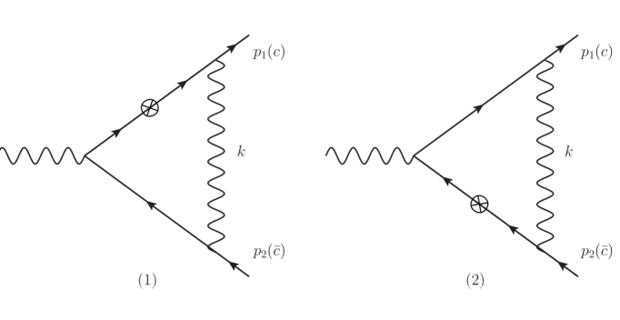
Figure 10: One loop diagrams with mass counter terms insertion.

The term $\mathcal{M}^{\mu}_{\rm CT,m}$ receives contributions from the two Feynman diagrams shown in fig. 10, where $k$ is the loop momentum and $\otimes$ denotes the mass counterterms. If $\otimes$ is added to the collinear (anticollinear) leg as shown in diagram (1) (diagram (2)) in fig. 10, it corresponds to a one-loop contribution in collinear (anticollinear) region. In addition to the mass counterterms, the two diagrams in fig. 10 represent the one-loop corrections induced by the loop momentum $k$. As discussed in sec. 3, this loop momentum $k$ can be hard, collinear or anticollinear, which corresponds to respectively the hard, collinear and anticollinear region. Only the latter two contribute to the collinear-anticollinear region at two-loop level. Moreover, the Feynman diagram with $\otimes$ being added to the anticollinear leg and $k$ being anticollinear contributes to the double-anticollinear region, while the Feynman diagram with $\otimes$ being added to the collinear leg and $k$ being collinear contributes to double-collinear region. On the r.h.s. of eq. (216), we therefore only need to consider the contribution from the anticollinear region in the Feynman diagram (1) and collinear region in the Feynman diagram (2). Their contributions to the form factor are given by

$$F^{(2),\rm CT,m}_{1,c\bar{c}} =2\left(\frac{\bar{\mu}^{2}}{m^{2}}\right)^{2\epsilon}\left[\frac{9}{\epsilon^{3}}+\frac{12}{\epsilon^{2}}+\frac{1}{\epsilon}\left(9\zeta_{2}+66\right)+92+12\zeta_{2}-6\zeta_{3}\right],$$

$$F^{(2),\rm CT,m}_{2,c\bar{c}} =2\left(\frac{\bar{\mu}^{2}}{m^{2}}\right)^{2\epsilon}\left[-\frac{6}{\epsilon^{3}}-\frac{20}{\epsilon^{2}}-\frac{1}{\epsilon}\left(6\zeta_{2}+56\right)-144-20\zeta_{2}+4\zeta_{3}\right]\,.$$ (219)

The factor of $2$ is because of symmetry between the two diagrams in fig. 10. Moreover, we only need to consider the mass renormalization of hard functions on the l.h.s. of eq. (216). Note that $H_{f,\bar{f}}^{(0)\mu}$, $H_{f\partial\gamma,\bar{f}\,\rho\sigma}^{(0)\mu}$, $H_{f,\bar{f}\partial\gamma\,\rho\sigma}^{(0)\mu}$ and $H_{f\gamma,\bar{f}\gamma\,\rho\sigma}^{(0)\mu}$ do not depend on the fermion mass $m$ explicitly. We therefore only need to consider the mass renormalization of the hard functions $H_{f\gamma,\bar{f}\,\rho}^{(1)\mu}$, defined in eq. (76), and $H_{f,\bar{f}\gamma\,\rho}^{(1)\mu}$. Together with the corresponding jet functions, we have

$$\mathcal{M}^{\mu}_{\rm fac,CT,m} =J_{f\gamma}^{(1)\rho}\left(m_{0}\to m\right)H_{f\gamma,\bar{f}\,\rho}^{(1)\mu}\left(m_{0}\to(Z_{m}-1)m\right)J^{(0)}_{\bar{f}}\left(m_{0}\to m\right)$$

$$+J^{(0)}_{f}\left(m_{0}\to m\right)H_{f,\bar{f}\gamma\,\rho}^{(1)\mu}\left(m_{0}\to(Z_{m}-1)m\right)J_{\bar{f}\gamma}^{(1)\rho}\left(m_{0}\to m\right)\,,$$ (220)

where the mass renormalization of jet functions is not involved as mentioned before. The contributions of $\mathcal{M}^{\mu}_{\rm fac,CT,m}$ to the form factors are given by

$$F^{(2),\rm fac,CT,m}_{1,c\bar{c}} =2\left(\frac{\bar{\mu}^{2}}{m^{2}}\right)^{2\epsilon}\left(-\frac{6}{\epsilon}-20\right)$$

$$F^{(2),\rm fac,CT,m}_{2,c\bar{c}} =0\,.$$ (221)

Substituting eqs. (D), (D) and (D) into eq. (217), we now conclude that our factorization formula indeed works in the $c\bar{c}$-region for the renormalized 1PI amplitude at two loops.

References

- (1) F. E. Low, Bremsstrahlung of very low-energy quanta in elementary particle collisions, Phys. Rev. 110 (1958) 974–977.
- (2) T. H. Burnett and N. M. Kroll, Extension of the low soft photon theorem, Phys. Rev. Lett. 20 (1968) 86.
- (3) V. Del Duca, High-energy bremsstrahlung theorems for soft photons, Nucl. Phys. B345 (1990) 369–388.
- (4) E. Laenen, L. Magnea, and G. Stavenga, On next-to-eikonal corrections to threshold resummation for the Drell-Yan and DIS cross sections, Phys. Lett. B669 (2008) 173–179, [arXiv:0807.4412].
- (5) E. Laenen, L. Magnea, G. Stavenga, and C. D. White, Next-to-eikonal corrections to soft gluon radiation: a diagrammatic approach, JHEP 1101 (2011) 141, [arXiv:1010.1860].
- (6) A. J. Larkoski, D. Neill, and I. W. Stewart, Soft theorems from effective field theory, JHEP 1506 (2015) 077, [arXiv:1412.3108].
- (7) D. Bonocore, E. Laenen, L. Magnea, L. Vernazza, and C. D. White, The method of regions and next-to-soft corrections in Drell-Yan production, Phys. Lett. B742 (2015) 375–382, [arXiv:1410.6406].
- (8) Y.-Q. Ma, J.-W. Qiu, G. Sterman, and H. Zhang, Factorized power expansion for high- heavy quarkonium production, Phys. Rev. Lett. 113 (2014), no. 14 142002, [arXiv:1407.0383].
- (9) Z.-B. Kang, Y.-Q. Ma, J.-W. Qiu, and G. Sterman, Heavy Quarkonium Production at Collider Energies: Partonic Cross Section and Polarization, Phys. Rev. D 91 (2015), no. 1 014030, [arXiv:1411.2456].
- (10) D. Bonocore, E. Laenen, L. Magnea, S. Melville, L. Vernazza, and C. D. White, A factorization approach to next-to-leading-power threshold logarithms, JHEP 06 (2015) 008, [arXiv:1503.05156].
- (11) D. Bonocore, E. Laenen, L. Magnea, L. Vernazza, and C. D. White, Non-abelian factorisation for next-to-leading-power threshold logarithms, JHEP 12 (2016) 121, [arXiv:1610.06842].
- (12) I. Moult, L. Rothen, I. W. Stewart, F. J. Tackmann, and H. X. Zhu, Subleading power corrections for N-jettiness subtractions, Phys. Rev. D95 (2017), no. 7 074023, [arXiv:1612.00450].
- (13) I. Feige, D. W. Kolodrubetz, I. Moult, and I. W. Stewart, A complete basis of helicity operators for subleading factorization, JHEP 1711 (2017) 142, [arXiv:1703.03411].
- (14) I. Moult, I. W. Stewart, and G. Vita, A subleading operator basis and matching for gg H, JHEP 1707 (2017) 067, [arXiv:1703.03408].
- (15) I. Moult, L. Rothen, I. W. Stewart, F. J. Tackmann, and H. X. Zhu, N -jettiness subtractions for at subleading power, Phys. Rev. D97 (2018), no. 1 014013, [arXiv:1710.03227].
- (16) H. Gervais, Soft photon theorem for high energy amplitudes in Yukawa and scalar theories, Phys. Rev. D95 (2017), no. 12 125009, [arXiv:1704.00806].
- (17) V. Del Duca, E. Laenen, L. Magnea, L. Vernazza, and C. D. White, Universality of next-to-leading power threshold effects for colourless final states in hadronic collisions, JHEP 11 (2017) 057, [arXiv:1706.04018].
- (18) M. Beneke, M. Garny, R. Szafron, and J. Wang, Anomalous dimension of subleading-power N-jet operators, JHEP 03 (2018) 001, [arXiv:1712.04416].
- (19) I. Moult, I. W. Stewart, G. Vita, and H. X. Zhu, First Subleading Power Resummation for Event Shapes, JHEP 08 (2018) 013, [arXiv:1804.04665].
- (20) M. Beneke, M. Garny, R. Szafron, and J. Wang, Anomalous dimension of subleading-power -jet operators. Part II, JHEP 11 (2018) 112, [arXiv:1808.04742].
- (21) M. Beneke, A. Broggio, M. Garny, S. Jaskiewicz, R. Szafron, L. Vernazza, and J. Wang, Leading-logarithmic threshold resummation of the Drell-Yan process at next-to-leading power, JHEP 1903 (2019) 043, [arXiv:1809.10631].
- (22) M. A. Ebert, I. Moult, I. W. Stewart, F. J. Tackmann, G. Vita, and H. X. Zhu, Power Corrections for N-Jettiness Subtractions at , JHEP 12 (2018) 084, [arXiv:1807.10764].
- (23) N. Bahjat-Abbas, D. Bonocore, J. Sinninghe Damsté, E. Laenen, L. Magnea, L. Vernazza, and C. White, Diagrammatic resummation of leading-logarithmic threshold effects at next-to-leading power, JHEP 11 (2019) 002, [arXiv:1905.13710].
- (24) I. Moult, I. W. Stewart, and G. Vita, Subleading Power Factorization with Radiative Functions, arXiv:1905.07411.
- (25) M. Beneke, M. Garny, R. Szafron, and J. Wang, Violation of the Kluberg-Stern-Zuber theorem in SCET, JHEP 09 (2019) 101, [arXiv:1907.05463].
- (26) M. Beneke, M. Garny, S. Jaskiewicz, R. Szafron, L. Vernazza, and J. Wang, Leading-logarithmic threshold resummation of Higgs production in gluon fusion at next-to-leading power, JHEP 01 (2020) 094, [arXiv:1910.12685].
- (27) Z. L. Liu and M. Neubert, Factorization at subleading power and endpoint-divergent convolutions in decay, JHEP 04 (2020) 033, [arXiv:1912.08818].
- (28) M. Beneke, A. Broggio, S. Jaskiewicz, and L. Vernazza, Threshold factorization of the Drell-Yan process at next-to-leading power, JHEP 07 (2020) 078, [arXiv:1912.01585].
- (29) M. van Beekveld, W. Beenakker, E. Laenen, and C. D. White, Next-to-leading power threshold effects for inclusive and exclusive processes with final state jets, JHEP 03 (2020) 106, [arXiv:1905.08741].
- (30) M. van Beekveld, W. Beenakker, R. Basu, E. Laenen, A. Misra, and P. Motylinski, Next-to-leading power threshold effects for resummed prompt photon production, Phys. Rev. D 100 (2019), no. 5 056009, [arXiv:1905.11771].
- (31) I. Moult, I. W. Stewart, G. Vita, and H. X. Zhu, The Soft Quark Sudakov, JHEP 05 (2020) 089, [arXiv:1910.14038].
- (32) Z. L. Liu and M. Neubert, Two-Loop Radiative Jet Function for Exclusive -Meson and Higgs Decays, JHEP 06 (2020) 060, [arXiv:2003.03393].
- (33) Z. L. Liu, B. Mecaj, M. Neubert, X. Wang, and S. Fleming, Renormalization and Scale Evolution of the Soft-Quark Soft Function, JHEP 07 (2020) 104, [arXiv:2005.03013].
- (34) A. H. Ajjath, P. Mukherjee, and V. Ravindran, Next to soft corrections to Drell-Yan and Higgs boson productions, Phys. Rev. D 105 (2022), no. 9 094035, [arXiv:2006.06726].
- (35) A. H. Ajjath, P. Mukherjee, V. Ravindran, A. Sankar, and S. Tiwari, On next to soft threshold corrections to DIS and SIA processes, JHEP 04 (2021) 131, [arXiv:2007.12214].
- (36) A. H. Ajjath, P. Mukherjee, V. Ravindran, A. Sankar, and S. Tiwari, Next-to-soft corrections for Drell-Yan and Higgs boson rapidity distributions beyond N3LO, Phys. Rev. D 103 (2021) L111502, [arXiv:2010.00079].
- (37) A. H. Ajjath, P. Mukherjee, V. Ravindran, A. Sankar, and S. Tiwari, Next-to SV resummed Drell–Yan cross section beyond leading-logarithm, Eur. Phys. J. C 82 (2022), no. 3 234, [arXiv:2107.09717].
- (38) M. Beneke, M. Garny, S. Jaskiewicz, R. Szafron, L. Vernazza, and J. Wang, Large-x resummation of off-diagonal deep-inelastic parton scattering from d-dimensional refactorization, JHEP 10 (2020) 196, [arXiv:2008.04943].
- (39) E. Laenen, J. Sinninghe Damsté, L. Vernazza, W. Waalewijn, and L. Zoppi, Towards all-order factorization of QED amplitudes at next-to-leading power, Phys. Rev. D 103 (2021), no. 3 034022, [arXiv:2008.01736].
- (40) Z. L. Liu, B. Mecaj, M. Neubert, and X. Wang, Factorization at subleading power, Sudakov resummation, and endpoint divergences in soft-collinear effective theory, Phys. Rev. D 104 (2021), no. 1 014004, [arXiv:2009.04456].
- (41) M. van Beekveld, E. Laenen, J. Sinninghe Damsté, and L. Vernazza, Next-to-leading power threshold corrections for finite order and resummed colour-singlet cross sections, JHEP 05 (2021) 114, [arXiv:2101.07270].
- (42) A. Broggio, S. Jaskiewicz, and L. Vernazza, Next-to-leading power two-loop soft functions for the Drell-Yan process at threshold, JHEP 10 (2021) 061, [arXiv:2107.07353].
- (43) M. van Beekveld, L. Vernazza, and C. D. White, Threshold resummation of new partonic channels at next-to-leading power, JHEP 12 (2021) 087, [arXiv:2109.09752].
- (44) D. Bonocore, A. Kulesza, and J. Pirsch, Classical and quantum gravitational scattering with Generalized Wilson Lines, JHEP 03 (2022) 147, [arXiv:2112.02009].
- (45) T. Engel, A. Signer, and Y. Ulrich, Universal structure of radiative QED amplitudes at one loop, JHEP 04 (2022) 097, [arXiv:2112.07570].
- (46) M. Beneke, M. Garny, S. Jaskiewicz, J. Strohm, R. Szafron, L. Vernazza, and J. Wang, Next-to-leading power endpoint factorization and resummation for off-diagonal “gluon” thrust, JHEP 07 (2022) 144, [arXiv:2205.04479].
- (47) G. Bell, P. Böer, and T. Feldmann, Muon-electron backward scattering: a prime example for endpoint singularities in SCET, JHEP 09 (2022) 183, [arXiv:2205.06021].
- (48) Z. L. Liu, M. Neubert, M. Schnubel, and X. Wang, Factorization at next-to-leading power and endpoint divergences in gg → h production, JHEP 06 (2023) 183, [arXiv:2212.10447].
- (49) T. Engel, The LBK theorem to all orders, JHEP 07 (2023) 177, [arXiv:2304.11689].
- (50) T. Engel, Multiple soft-photon emission at next-to-leading power to all orders, JHEP 03 (2024) 004, [arXiv:2311.17612].
- (51) A. Broggio, S. Jaskiewicz, and L. Vernazza, Threshold factorization of the Drell-Yan quark-gluon channel and two-loop soft function at next-to-leading power, arXiv:2306.06037.
- (52) M. van Beekveld, A. Danish, E. Laenen, S. Pal, A. Tripathi, and C. D. White, Next-to-soft radiation from a different angle, Phys. Rev. D 109 (2024), no. 7 074005, [arXiv:2308.12850].
- (53) M. van Beekveld, L. Vernazza, and C. D. White, Exponentiation of soft quark effects from the replica trick, JHEP 07 (2024) 109, [arXiv:2312.11606].
- (54) R. Balsach, D. Bonocore, and A. Kulesza, Soft-photon spectra and the Low-Burnett-Kroll theorem, Phys. Rev. D 110 (2024), no. 1 016029, [arXiv:2312.11386].
- (55) M. Beneke, Y. Ji, and X. Wang, Renormalization of the next-to-leading-power → h and gg → h soft quark functions, JHEP 05 (2024) 246, [arXiv:2403.17738].
- (56) M. Beneke, Y. Ji, E. Sünderhauf, and X. Wang, Renormalization of the Next-to-Leading-Power Soft Function for the Drell-Yan Off-diagonal Channel, arXiv:2502.01973.
- (57) A. H. Mueller, On the asymptotic behavior of the sudakov form-factor, Phys. Rev. D20 (1979) 2037.
- (58) J. C. Collins, Algorithm to compute corrections to the sudakov form- factor, Phys. Rev. D22 (1980) 1478.
- (59) J. C. Collins and D. E. Soper, Back to back jets in qcd, Nucl. Phys. B193 (1981) 381.
- (60) A. Sen, Asymptotic behavior of the sudakov form-factor in qcd, Phys. Rev. D24 (1981) 3281.
- (61) J. C. Collins, Sudakov form-factors, Adv.Ser.Direct.High Energy Phys. 5 (1989) 573–614, [hep-ph/0312336].
- (62) L. J. Dixon, L. Magnea, and G. F. Sterman, Universal structure of subleading infrared poles in gauge theory amplitudes, JHEP 0808 (2008) 022, [arXiv:0805.3515].
- (63) S. M. Aybat, L. J. Dixon, and G. F. Sterman, The Two-loop soft anomalous dimension matrix and resummation at next-to-next-to leading pole, Phys. Rev. D74 (2006) 074004, [hep-ph/0607309].
- (64) E. Gardi and L. Magnea, Factorization constraints for soft anomalous dimensions in QCD scattering amplitudes, JHEP 0903 (2009) 079, [arXiv:0901.1091].
- (65) T. Becher and M. Neubert, On the Structure of Infrared Singularities of Gauge-Theory Amplitudes, JHEP 0906 (2009) 081, [arXiv:0903.1126].
- (66) L. Magnea and G. F. Sterman, Analytic continuation of the Sudakov form-factor in QCD, Phys. Rev. D42 (1990) 4222–4227.
- (67) H. Contopanagos, E. Laenen, and G. F. Sterman, Sudakov factorization and resummation, Nucl. Phys. B 484 (1997) 303–330, [hep-ph/9604313].
- (68) N. Kidonakis and G. Sterman, Resummation for qcd hard scattering, Nucl. Phys. B505 (1997) 321–348, [hep-ph/9705234].
- (69) N. Kidonakis, G. Oderda, and G. Sterman, Threshold resummation for dijet cross-sections, Nucl. Phys. B525 (1998) 299, [hep-ph/9801268].
- (70) L. Magnea, Analytic resummation for the quark form-factor in QCD, Nucl. Phys. B 593 (2001) 269–288, [hep-ph/0006255].
- (71) S. Catani, S. Dittmaier, and Z. Trocsanyi, One loop singular behavior of QCD and SUSY QCD amplitudes with massive partons, Phys. Lett. B 500 (2001) 149–160, [hep-ph/0011222].
- (72) A. A. Penin, Two-loop photonic corrections to massive Bhabha scattering, Nucl. Phys. B 734 (2006) 185–202, [hep-ph/0508127].
- (73) A. A. Penin, Two-loop corrections to Bhabha scattering, Phys. Rev. Lett. 95 (2005) 010408, [hep-ph/0501120].
- (74) A. Mitov and S. Moch, The Singular behavior of massive QCD amplitudes, JHEP 05 (2007) 001, [hep-ph/0612149].
- (75) T. Becher and K. Melnikov, Two-loop QED corrections to Bhabha scattering, JHEP 06 (2007) 084, [arXiv:0704.3582].
- (76) M. Czakon, A. Mitov, and S. Moch, Heavy-quark production in massless quark scattering at two loops in QCD, Phys. Lett. B 651 (2007) 147–159, [arXiv:0705.1975].
- (77) M. Czakon, A. Mitov, and S. Moch, Heavy-quark production in gluon fusion at two loops in QCD, Nucl. Phys. B 798 (2008) 210–250, [arXiv:0707.4139].
- (78) A. Mitov, G. F. Sterman, and I. Sung, The Massive Soft Anomalous Dimension Matrix at Two Loops, Phys. Rev. D79 (2009) 094015, [arXiv:0903.3241].
- (79) T. Becher and M. Neubert, Infrared singularities of QCD amplitudes with massive partons, Phys. Rev. D79 (2009) 125004, [arXiv:0904.1021].
- (80) P. Banerjee, T. Engel, A. Signer, and Y. Ulrich, QED at NNLO with McMule, SciPost Phys. 9 (2020) 027, [arXiv:2007.01654].
- (81) G. Wang, T. Xia, L. L. Yang, and X. Ye, On the high-energy behavior of massive QCD amplitudes, JHEP 05 (2024) 082, [arXiv:2312.12242].
- (82) G. Wang, T. Xia, L. L. Yang, and X. Ye, Two-loop QCD amplitudes for production from boosted limit, JHEP 07 (2024) 121, [arXiv:2402.00431].
- (83) G. Sterman, Summation of large corrections to short distance hadronic cross-sections, Nucl. Phys. B281 (1987) 310.
- (84) S. Catani and L. Trentadue, Resummation of the QCD perturbative series for hard processes, Nucl. Phys. B327 (1989) 323.
- (85) S. Catani and L. Trentadue, Comment on qcd exponentiation at large x, Nucl. Phys. B353 (1991) 183–186.
- (86) G. P. Korchemsky and G. Marchesini, Structure function for large x and renormalization of wilson loop, Nucl. Phys. B406 (1993) 225–258, [hep-ph/9210281].
- (87) G. P. Korchemsky and G. Marchesini, Resummation of large infrared corrections using Wilson loops, Phys. Lett. B313 (1993) 433–440.
- (88) C. W. Bauer, S. Fleming, D. Pirjol, and I. W. Stewart, An effective field theory for collinear and soft gluons: Heavy to light decays, Phys. Rev. D63 (2001) 114020, [hep-ph/0011336].
- (89) C. W. Bauer, D. Pirjol, and I. W. Stewart, Soft collinear factorization in effective field theory, Phys. Rev. D 65 (2002) 054022, [hep-ph/0109045].
- (90) M. Beneke, A. P. Chapovsky, M. Diehl, and T. Feldmann, Soft collinear effective theory and heavy to light currents beyond leading power, Nucl. Phys. B 643 (2002) 431–476, [hep-ph/0206152].
- (91) I. Moult, I. W. Stewart, F. J. Tackmann, and W. J. Waalewijn, Employing Helicity Amplitudes for Resummation, Phys. Rev. D 93 (2016), no. 9 094003, [arXiv:1508.02397].
- (92) D. W. Kolodrubetz, I. Moult, and I. W. Stewart, Building blocks for subleading helicity operators, JHEP 1605 (2016) 139, [arXiv:1601.02607].
- (93) J.-w. Qiu and G. F. Sterman, Power corrections in hadronic scattering. 1. Leading 1/Q**2 corrections to the Drell-Yan cross-section, Nucl. Phys. B 353 (1991) 105–136.
- (94) J.-w. Qiu and G. F. Sterman, Power corrections to hadronic scattering. 2. Factorization, Nucl. Phys. B 353 (1991) 137–164.
- (95) W. Bernreuther, R. Bonciani, T. Gehrmann, R. Heinesch, T. Leineweber, P. Mastrolia, and E. Remiddi, Two-loop QCD corrections to the heavy quark form-factors: The Vector contributions, Nucl. Phys. B 706 (2005) 245–324, [hep-ph/0406046].
- (96) J. Gluza, A. Mitov, S. Moch, and T. Riemann, The QCD form factor of heavy quarks at NNLO, JHEP 07 (2009) 001, [arXiv:0905.1137].
- (97) J. Blümlein, A. De Freitas, C. Raab, and K. Schönwald, The initial state QED corrections to , Nucl. Phys. B 956 (2020) 115055, [arXiv:2003.14289].
- (98) J. M. Henn, A. V. Smirnov, and V. A. Smirnov, Analytic results for planar three-loop integrals for massive form factors, JHEP 12 (2016) 144, [arXiv:1611.06523].
- (99) J. Henn, A. V. Smirnov, V. A. Smirnov, and M. Steinhauser, Massive three-loop form factor in the planar limit, JHEP 01 (2017) 074, [arXiv:1611.07535].
- (100) J. Ablinger, A. Behring, J. Blümlein, G. Falcioni, A. De Freitas, P. Marquard, N. Rana, and C. Schneider, Heavy quark form factors at two loops, Phys. Rev. D 97 (2018), no. 9 094022, [arXiv:1712.09889].
- (101) R. N. Lee, A. V. Smirnov, V. A. Smirnov, and M. Steinhauser, Three-loop massive form factors: complete light-fermion corrections for the vector current, JHEP 03 (2018) 136, [arXiv:1801.08151].
- (102) R. N. Lee, A. V. Smirnov, V. A. Smirnov, and M. Steinhauser, Three-loop massive form factors: complete light-fermion and large-Nc corrections for vector, axial-vector, scalar and pseudo-scalar currents, JHEP 05 (2018) 187, [arXiv:1804.07310].
- (103) J. Ablinger, J. Blümlein, P. Marquard, N. Rana, and C. Schneider, Heavy quark form factors at three loops in the planar limit, Phys. Lett. B 782 (2018) 528–532, [arXiv:1804.07313].
- (104) J. Blümlein, P. Marquard, and N. Rana, Asymptotic behavior of the heavy quark form factors at higher order, Phys. Rev. D 99 (2019), no. 1 016013, [arXiv:1810.08943].
- (105) J. Blümlein, P. Marquard, N. Rana, and C. Schneider, The Heavy Fermion Contributions to the Massive Three Loop Form Factors, Nucl. Phys. B 949 (2019) 114751, [arXiv:1908.00357].
- (106) M. Fael, F. Lange, K. Schönwald, and M. Steinhauser, Massive Vector Form Factors to Three Loops, Phys. Rev. Lett. 128 (2022), no. 17 172003, [arXiv:2202.05276].
- (107) M. Fael, F. Lange, K. Schönwald, and M. Steinhauser, Singlet and nonsinglet three-loop massive form factors, Phys. Rev. D 106 (2022), no. 3 034029, [arXiv:2207.00027].
- (108) M. Fael, F. Lange, K. Schönwald, and M. Steinhauser, Massive three-loop form factors: Anomaly contribution, Phys. Rev. D 107 (2023), no. 9 094017, [arXiv:2302.00693].
- (109) J. Blümlein, A. De Freitas, P. Marquard, N. Rana, and C. Schneider, Analytic results on the massive three-loop form factors: Quarkonic contributions, Phys. Rev. D 108 (2023), no. 9 094003, [arXiv:2307.02983].
- (110) J. ter Hoeve, E. Laenen, C. Marinissen, L. Vernazza, and G. Wang, Region analysis of QED massive fermion form factor, JHEP 02 (2024) 024, [arXiv:2311.16215].
- (111) I. Hönemann, K. Tempest, and S. Weinzierl, Electron self-energy in QED at two loops revisited, Phys. Rev. D 98 (2018), no. 11 113008, [arXiv:1811.09308]. [Erratum: Phys.Rev.D 110, 059901 (2024)].
- (112) R. J. Hill and M. Neubert, Spectator interactions in soft collinear effective theory, Nucl. Phys. B 657 (2003) 229–256, [hep-ph/0211018].
- (113) L. Magnea, E. Maina, G. Pelliccioli, C. Signorile-Signorile, P. Torrielli, and S. Uccirati, Factorisation and Subtraction beyond NLO, JHEP 12 (2018) 062, [arXiv:1809.05444].
- (114) T. Becher and M. D. Schwartz, Direct photon production with effective field theory, JHEP 02 (2010) 040, [arXiv:0911.0681].
- (115) T. Becher and G. Bell, The gluon jet function at two-loop order, Phys. Lett. B 695 (2011) 252–258, [arXiv:1008.1936].
- (116) W. H. Furry, A symmetry theorem in the positron theory, Phys. Rev. 51 (Jan, 1937) 125–129.
- (117) J. Klappert, F. Lange, P. Maierhöfer, and J. Usovitsch, Integral reduction with Kira 2.0 and finite field methods, Comput. Phys. Commun. 266 (2021) 108024, [arXiv:2008.06494].
- (118) P. Maierhöfer, J. Usovitsch, and P. Uwer, Kira—A Feynman integral reduction program, Comput. Phys. Commun. 230 (2018) 99–112, [arXiv:1705.05610].
- (119) J. A. M. Vermaseren, New features of form, math-ph/0010025.
- (120) B. Ruijl, T. Ueda, and J. Vermaseren, FORM version 4.2, arXiv:1707.06453.
- (121) J. A. M. Vermaseren, Harmonic sums, Mellin transforms and integrals, Int. J. Mod. Phys. A 14 (1999) 2037–2076, [hep-ph/9806280].
- (122) M. Czakon, Automatized analytic continuation of Mellin-Barnes integrals, Comput. Phys. Commun. 175 (2006) 559–571, [hep-ph/0511200].
- (123) M. Ochman and T. Riemann, MBsums - a Mathematica package for the representation of Mellin-Barnes integrals by multiple sums, Acta Phys. Polon. B46 (2015), no. 11 2117, [arXiv:1511.01323].
- (124) T. Huber and D. Maitre, HypExp: A Mathematica package for expanding hypergeometric functions around integer-valued parameters, Comput. Phys. Commun. 175 (2006) 122–144, [hep-ph/0507094].
- (125) T. Becher and G. Bell, Analytic Regularization in Soft-Collinear Effective Theory, Phys. Lett. B 713 (2012) 41–46, [arXiv:1112.3907].
- (126) S. Gritschacher, A. Hoang, I. Jemos, and P. Pietrulewicz, Two loop soft function for secondary massive quarks, Phys. Rev. D 89 (2014), no. 1 014035, [arXiv:1309.6251].
- (127) J. Grammer, G. and D. Yennie, Improved treatment for the infrared divergence problem in quantum electrodynamics, Phys. Rev. D8 (1973) 4332–4344.