Fixed-Point RNNs: From Diagonal to Dense in a Few Iterations

Abstract

Linear recurrent neural networks (RNNs) and state-space models (SSMs) such as Mamba have become promising alternatives to softmax-attention as sequence mixing layers in Transformer architectures. Current models, however, do not exhibit the full state-tracking expressivity of RNNs because they rely on channel-wise (i.e. diagonal) sequence mixing. In this paper, we propose to compute a dense linear RNN as the fixed-point of a parallelizable diagonal linear RNN in a single layer. We explore mechanisms to improve its memory and state-tracking abilities in practice, and achieve state-of-the-art results on the commonly used toy tasks $A_{5}$, $S_{5}$, copying, and modular arithmetics. We hope our results will open new avenues to more expressive and efficient sequence mixers.

1 Introduction

State-space models (SSMs) and other new efficient recurrent token mixers are becoming a popular alternative to softmax attention in language modeling (Gu & Dao, 2023) as well as other applications such as vision (Liu et al., 2024), audio (Goel et al., 2022) and DNA processing (Nguyen et al., 2024). Inspired by linear input-controlled filtering, these models can be expressed as carefully parametrized linear recurrent neural networks (RNNs) with input-dependent, diagonal state transition: $h_{t}=\text{diag}(\mathbf{a}_{t})h_{t-1}+\mathbf{B}_{t}x_{t}$.

Compared to classical RNNs such as LSTMs, the recurrence from the previous hidden state $h_{t-1}$ to the current $h_{t}$ is linear and its coefficient $\mathbf{a}_{t}$ does not depend on the hidden states. These factors allow SSMs such as Mamba to be computed through efficient parallel methods during training. At test time, they are faster than classical Transformers on long sequences due to their recurrent nature.

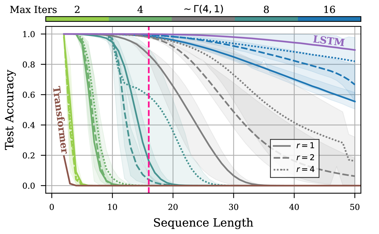
Figure 1: Sequence length generalization at training length 16 (pink) for state-tracking on $A_{5}$, with Transformer (brown) and LSTM (purple) as lower/upper bounds. Our Fixed-Point RNN (Bedouin) is trained at different maximum number of fixed-point iterations $\ell_{\text{max}}$: between $2$ (green) and $16$ (blue), or sampled from $\Gamma(4,1)$ with mean $4$ (gray). Increasing the number of fixed-point iterations turns the linear RNN from diagonal to dense in a few iterations.

Though modern linear RNNs have shown promise in practice, recent theoretical studies suggest that using dense transition matrices (i.e. replacing $\text{diag}(\mathbf{a}_{t})$ with a dense $\mathbf{A}_{t}$) could present an opportunity to improve expressivity and unlock performance on challenging tasks. In particular, Cirone et al. (2024b) prove that dense linear SSMs/RNNs are endowed with the theoretical expressivity of classical non-linear RNNs such as LSTMs. As shown by Merrill et al. (2024), this is particularly useful in state-tracking applications where models are expected to maintain and extrapolate a complex state of the world. While state-tracking is naturally expressed in non-linear RNNs, it is known to be unavailable to channel-wise sequence mixers such as SSMs or Transformers (Merrill & Sabharwal, 2023). Finally, DeltaNet demonstrated that controlled, non-diagonal state updates significantly improve learning of compressed associative memories (Schlag et al., 2021a; Yang et al., 2024b).

Although linear recurrences are parallelizable across sequence length (Martin & Cundy, 2018), parallelizing dense RNNs efficiently is not trivial. Because channels and tokens need to be mixed jointly, structured transition matrices such as head-wise WY-representations (Yang et al., 2024b), are required for efficient implementations. But mixing only within heads reduces expressivity. In this paper, we present a general recipe to parametrize a large class of selective dense linear RNNs as fixed-points of diagonal linear RNNs.

Fixed-point RNNs.

In order to understand the relationship between dense linear RNNs and the fixed point of diagonal linear RNNs, consider the recurrent form of a dense RNN

$$h^{*}_{t}=\mathbf{A}_{t}h^{*}_{t-1}+\mathbf{B}_{t}x_{t},$$ (1)

where $\mathbf{A}_{t}\in\mathbb{R}^{d\times d}$ corresponds to the state transition matrix, $\mathbf{B}_{t}\in\mathbb{R}^{d\times d}$ corresponds to the input transition matrix, $h^{*}_{t}\in\mathbb{R}^{d}$ corresponds to the hidden state, and $x_{t}\in\mathbb{R}^{d}$ corresponds to the input for $t<T$ steps.

We parametrize the state transition matrix $\mathbf{A}_{t}$ as the product of a diagonal matrix $\Lambda_{t}\in\mathbb{R}^{d\times d}$, and a non-diagonal invertible mixing matrix $\mathbf{Q}_{t}\in\mathbb{R}^{d\times d}$

$$h^{*}_{t}=\mathbf{Q}^{-1}_{t}\Lambda_{t}h^{*}_{t-1}+\mathbf{B}_{t}x_{t}.$$ (2)

For the diagonal linear RNN $f_{\theta}(x,h)$, we use $\Lambda_{t}$ as the diagonal state transition matrix, and $\mathbf{Q}_{t}\mathbf{B}_{t}$ resp. $(\mathbf{I}-\mathbf{Q}_{t})$ as transition matrices for its two input sequences $x$ and $h$:

$$f_{\theta}(x,h)_{t}=\Lambda_{t}f_{\theta}(x,h)_{t-1}+\mathbf{Q}_{t}\mathbf{B}_{t}x_{t}+(\mathbf{I}-\mathbf{Q}_{t})h_{t}.$$ (3)

Assuming that the diagonal linear RNN has a fixed-point in depth $h^{*}=f_{\theta}(x,h^{*})\in\mathbb{R}^{T\times d}$, we can first reformulate

$$h_{t}^{*} =\Lambda_{t}h_{t-1}^{*}+\mathbf{Q}_{t}\mathbf{B}_{t}x_{t}+(\mathbf{I}-\mathbf{Q}_{t})h_{t}^{*}$$

$$\mathbf{Q}_{t}h_{t}^{*} =\Lambda_{t}h_{t-1}^{*}+\mathbf{Q}_{t}\mathbf{B}_{t}x_{t},$$

and than multiply both sides by $\mathbf{Q}_{t}^{-1}$ to obtain equation (2). This means that the states of the dense linear RNN are implicitly described by the fixed-point of $f_{\theta}(x,h)$ if it exists. Therefore, we can compute a dense linear RNN by finding the fixed-point of the corresponding diagonal linear RNN.

Motivated by this insight, we carefully parametrize the diagonal RNN and its channel mixer $\mathbf{Q}_{t}$ such that a fixed-point iteration converges towards the hidden states of the dense RNN. Intuitively, this introduces an iteration in depth of interleaved channel mixing with $\mathbf{Q}_{t}$ and sequence mixing with parallelizable linear recurrences (Martin & Cundy, 2018).

Contributions.

In this work, we propose a recipe to design a general class of dense linear RNNs as fixed points of corresponding diagonal linear RNNs. Our contributions are:

1. We develop a framework for Fixed-Point RNNs and establish its inherent compatibility with linear attention.

2. Fixed-Point RNNs trade parallelism for expressivity with the number of fixed point iterations (Figure 1).

3. Fixed-Point RNNs unite previously isolated capabilities of recurrent computation and memory (Figure 2).

Outline.

After discussing related work in Sec. 2, we introduce the fixed-point RNN framework in Sec. 3, and explore mechanisms for copying in Sec. 4. In Sec. 5, we apply the framework to Mamba and evaluate it in Sec. 6.

2 Related Work

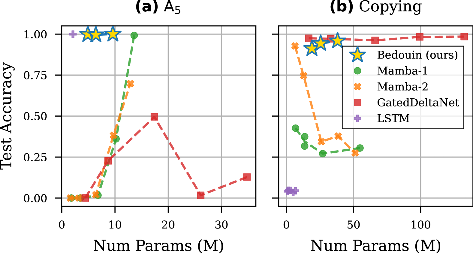
Figure 2: (a) State-tracking on $A_{5}$ at sequence length $16$, and (b) character accuracy of copying at $2\times$ sequence length generalization, trained on lengths $\in[5,50]$. Our single layer Fixed-Point RNN (Bedouin) with mixer reflections $r\in\{1,2,4\}$ is compared to baselines of increasing depth $\in\{1,2,4,6,8\}$. Bedouin is the only model capable of solving both the state-tracking and the copy task.

Since their introduction (Rumelhart et al., 1986; Elman, 1990), RNNs have significantly contributed to the evolution of machine learning methods for sequential data, marked by key innovations such as the LSTM (Hochreiter & Schmidhuber, 1997) and Echo-State Networks (Jaeger, 2001). However, two significant challenges lead to the widespread adoption of the Transformer architecture (Vaswani et al., 2017): first, GPU hardware is optimized for large-scale matrix multiplications. Second, recurrent models are notoriously difficult to train due to vanishing and exploding gradients (Hochreiter et al., 2001; Pascanu et al., 2013).

Beyond softmax attention.

The quadratic runtime complexity of Transformers motivated research on the linearization of its attention mechanism (Wang et al., 2020; Chen et al., 2021; Choromanski et al., 2020) – a technique that inevitably brings the sequence mixing mechanism closer to RNN-like processing (Katharopoulos et al., 2020; Schlag et al., 2021b). Recently, improvements on the long-range-arena benchmark (Tay et al., 2020) with state-space models (Gu et al., 2022; Smith et al., 2023) sparked a renewed interest in recurrent models (Gu & Dao, 2023; Sun et al., 2023; De et al., 2024; Qin et al., 2024; Peng et al., 2024; Yang et al., 2024a). New efficient token mixing strategies such as Mamba (Gu & Dao, 2023) showcase impressive results in language modeling (Waleffe et al., 2024) while offering linear runtime complexity. These models are fundamentally diagonal linear RNNs, which enables parallel algorithms such as parallel scans (Martin & Cundy, 2018) and fast linear attention based implementations (Yang et al., 2024b; Dao & Gu, 2024).

Expressivity of Diagonal vs. Dense RNNs.

It was recently pointed out by Cirone et al. (2024b) that the diagonality in the hidden-to-hidden state transition inevitably causes expressivity issues, showcasing a stark distinction with classic dense nonlinear RNNs, known to be Turing-complete (Siegelmann & Sontag, 1992; Korsky, 2019) and fully expressive in a dynamical systems sense (Hanson & Raginsky, 2020).  Merrill et al. (2024) pointed at a similar issue with diagonality using tools from circuit complexity: in contrast to e.g. LSTMs, diagonal linear RNNs can not express state-tracking algorithms. This issue sparked interest in designing fast non-diagonal recurrent mechanisms and, more generally, in providing architectures capable of solving state-tracking problems. The first example of such an architecture is DeltaNet (Yang et al., 2024b) employing a parallelizable Housholder reflection as a state transition matrix. Endowing this matrix with negative eigenvalues improves tracking in SSMs (Grazzi et al., 2024). In concurrent work, Siems et al. (2025) show that adding more reflections improves state-tracking.

Toy tasks.

Several works propose toy tasks to identify specific shortcomings of modern architectures. Specifically, Beck et al. (2024) use the Chomsky hierarchy to organize formal language tasks, of which a modular arithmetic task remains unsolved. With similar motivations, Merrill & Sabharwal (2023) introduce a set of word-problems for assessing state-tracking capabilities, among which the $A_{5}$ and $S_{5}$ tasks remain unsolved by Transformers and SSMs. Motivated by Transformers outperforming RNNs in memory capabilities, Jelassi et al. (2024) introduce a copying task as a fundamental benchmark for memory. We focus on these tasks to evaluate our Fixed-Point RNN framework.

Recurrence in Depth.

Machine learning models that reduce an intrinsic energy through iterations have been an object of interest for decades (Hopfield, 1982; Miyato et al., 2025). For example, recurrence in depth can increase the expressivity of Transformers (Dehghani et al., 2019; Schwarzschild et al., 2021; Giannou et al., 2023) and is sometimes also understood as adaptive compute time (Graves, 2016). Under certain assumptions, iterated blocks can converge to an equilibrium point where they implicitly describe an expressive function (Bai et al., 2019; Ghaoui et al., 2021). Recently, this technique has been used to approximate non-linear RNNs with a fixed-point iteration of parallelizable linear RNNs (Lim et al., 2024; Gonzalez et al., 2024). In concurrent work to ours, Schöne et al. (2025) apply an iteration in depth to Mamba-2 and Llama blocks to increase expressivity and show promising results of their implicit language models. In contrast, we derive an explicit fixed-point iteration towards a dense linear RNN with a theoretically motivated parameterization, and focus on theoretical toy tasks.

3 Fixed-Points as an RNN Layer

In this section, we first parametrize a diagonal linear RNN that is guaranteed to have an attracting fixed-point (Sec. 3.1). Then, we show that for the backward pass, it suffices to compute gradients only at the fixed-point $h^{*}$ itself (Sec. 3.2).

3.1 Computing the fixed point

Solving fixed-point equations such as $h=f_{\theta}(x,h)$, as needed from our discussion of (3), is perhaps one of the most well-studied problems in mathematics (Granas et al., 2003), often appearing in the fields of functional analysis and optimization. A common option in deep learning, used e.g. to find fixed points in deep equilibrium models (Bai et al., 2019), is Broyden's method (Broyden, 1965). While much more efficient than standard optimization due to the lack of reliance on backward passes, Broyden's method requires extra memory to keep track of the changes in the hidden state and is vulnerable to poorly conditioned curvatures (Bai et al., 2021; Martens, 2020).

However, focusing for the time being on the forward pass (see our discussion in Sec. 3.2 for the backward pass), a straightforward and yet effective method to compute the fixed point of an operator is simply to roll out the fixed point iteration. In the context of solving $h^{*}=f_{\theta}(x,h^{*})$, this corresponds to introducing an iteration in depth to (3). We introduce the superscript $\ell$ to the hidden state as $h_{t}^{\ell}$, where $t$ denotes the index of the current token (i.e., over the sequence dimension) and $\ell$ denotes the current iteration in depth (i.e., over the layer dimension) and compute $h_{t}^{\ell}$ from $h_{t}^{\ell-1}$ with $h_{t}^{0}=0$ as

$$h_{t}^{\ell}=\Lambda_{t}h_{t-1}^{{\ell-1}}+\mathbf{Q}_{t}\mathbf{B}_{t}x_{t}+(\mathbf{I}-\mathbf{Q}_{t})h_{t}^{\ell-1}.$$ (4)

The difficulty with such an iteration in time and depth is that, without any further constraint, it is prone to instabilities – due to the fact that fixed points might not exist or be unstable (Granas et al., 2003). While direct normalization techniques such as Layer Normalization might prevent from divergence (Beck et al., 2024), we here seek a more grounded alternative. Towards deriving a stable recurrence in depth, we make use of Banach's fixed point theorem (Banach, 1922), that provides sufficient conditions for an operator to have an attracting fixed point:

Theorem 3.1.

[Banach (1922)] Let $T(\cdot)$ be an operator with Lipschitz constant $\lambda_{T}<1$. Then, for any starting point the fixed point iteration method will converge to the fixed point of $T(\cdot)$ at rate $\mathcal{O}\left(1/\lambda_{T}\right)$.

While Banach's theorem has been used in the context of fixed point of neural networks before (Fung et al., 2022), in this paper we are specifically focusing on recurrent models. Based on the result of Theorem 3.1, we present the following theorem for stabilizing diagonal linear RNNs:

Theorem 3.2.

Let $f_{\theta}(x,h)$ be the diagonal linear RNN

$$f_{\theta}(x,h)_{t}=\Lambda f_{\theta}(x,h)_{t-1}+\left(\mathbf{I}-\Lambda\right)\left(\mathbf{Q}\mathbf{B}_{t}x_{t}+\left(\mathbf{I}-\mathbf{Q}\right)h_{t}\right),$$

where $\Lambda$ and $\mathbf{Q}$ are input-independent matrices and $\Lambda$ is diagonal. If $\Lambda$ and $\mathbf{I}-\mathbf{Q}$ are contractive (i.e. $\|\cdot\|_{2}<1$), then $f_{\theta}(x,h)$ has a Lipschitz constant $<1$ in $h$. Proof in App. A.

Theorem 3.2 provides a way to parametrize linear RNNs with input-independent transition matrices in order to ensure the latent iterated operator has Lipschitz constant $<1$: the recurrence in time is stabilized using a contractive state transition matrix $\Lambda$ and a coupled input normalization $\mathbf{I}-\Lambda$ (cf. discussion in (Zucchet & Orvieto, 2024)). Next, For stable recurrence in depth, the input transition matrix acting on $h$ is set to be contractive. This guarantees that throughout the fixed-point iteration, all sequences $h^{\ell}$ up to $h^{*}$ do not explode.

3.2 Computing the gradient

One advantage of an explicit fixed-point parameterization, such as the one derived in Theorem 3.2, lies in the gradient computation. As described by Bai et al. (2019), back-propagation through the fixed-point iteration can be avoided once a fixed-point is found. To see this, consider the Jacobian across $\ell$ iterations $\mathbf{J}_{x}^{\ell}=\frac{\partial f_{\theta}}{\partial x}(x,h^{\ell-1})$. Since $h^{\ell-1}$ depends on $x$ as well, we can recursively express $\mathbf{J}_{x}^{\ell}$ in terms of $\mathbf{J}_{x}^{\ell-1}$ and the Jacobians of a single iteration $\mathbf{J}_{x}(h)=\frac{\partial f_{\theta}}{\partial x}(x,h)$ and $\mathbf{J}_{h}=\frac{\partial f_{\theta}}{\partial h}(x,h)$ by applying the chain rule

$$\mathbf{J}_{x}^{\ell}=\mathbf{J}_{x}(h^{\ell-1})+\mathbf{J}_{h^{\ell-1}}\cdot\mathbf{J}_{x}^{\ell-1}.$$

Instead of unrolling, we can implicitly differentiate $h^{*}=f_{\theta}(x,h^{*})$ w.r.t. $x$, which yields $\mathbf{J}_{x}^{*}=\mathbf{J}_{x}(h^{*})+\mathbf{J}_{h^{*}}\cdot\mathbf{J}_{x}^{*}$. Given the conditions on the Lipschitz constant of $f_{\theta}(x,h)$ in $h$, we can assume $\mathbf{J}_{h^{\ell}}$ to be contractive and therefore $\left(\mathbf{I}-\mathbf{J}_{h^{\ell}}\right)$ to be positive definite and invertible. This allows to reformulate as

$$\mathbf{J}_{x}^{*}=(\mathbf{I}-\mathbf{J}_{h^{*}})^{-1}\cdot\mathbf{J}_{x}(h^{*}).$$ (5)

The case for $\mathbf{J}_{\theta}^{*}$ works analogously. This means that the gradient w.r.t. the input $x$ and parameters $\theta$ can be computed at the fixed-point with the cost of solving $(\mathbf{I}-\mathbf{J}_{h^{*}})^{-1}$. Bai et al. (2021) and Schöne et al. (2025) approximate this inverse using the first terms of the Neumann series, which leads to a truncated backpropagation formulation or phantom gradients, incurring sequential overhead. We avoid this inversion altogether with the following workaround:

Theorem 3.3.

Let $f_{\theta}(x,h)$ be a diagonal linear RNN, with fixed-point $h^{*}$ and Lipschitz constant $<1$ in $h$. Let further $\mathcal{L}(\cdot,\cdot)$ be a loss and $y$ a target. If the Jacobians $\mathbf{J}_{x}(h)=\frac{\partial f_{\theta}}{\partial x}\left(x,h\right)$ and $\mathbf{J}_{h}=\frac{\partial f_{\theta}}{\partial h}\left(x,h\right)$ are equal, then the gradient $\nabla_{\theta}\mathcal{L}(f_{\theta}(x,h),y)$ computed at the fixed point $h=h^{*}$ will be a descent direction of $\mathcal{L}\left(f_{\theta}(x,h^{*}),y\right)$. Proof in App. B.

Similar to  (Fung et al., 2022), Theorem 3.3 shows that parametrizing $f_{\theta}(x,h)$ such that $\mathbf{J}_{x}(h)=\mathbf{J}_{h}$ guarantees optimization progress even if the gradient is computed only at the fixed-point. In practice, we observe that adhering to this condition speeds-up the convergence of the model during training.

3.3 Parameterization of the mixer $\mathbf{Q}_{t}$

In Sec. 3, we showed how to design diagonal linear recurrences that converge to a dense linear RNN via fixed-point iterations and how to train them. In this section, we turn our attention to the fixed-point dense object, and discuss a choice for $\mathbf{Q}_{t}$, where $\mathbf{A}_{t}=\mathbf{Q}^{-1}_{t}\Lambda_{t}$ as in (2), striking a balance between parameter efficiency and expressivity.

According to (Cirone et al., 2024b; Merrill et al., 2024), a key factor to increase expressivity in dense linear RNNs lies in effectively mixing information through the hidden state’s dimensions. While using a non-structured input-dependent state transition matrix would be prohibitive both computationally and in terms of required parameters with $\mathcal{O}\left(d^{3}\right)$ cost, certain structures such as circulant matrices do not improve the expressivity due to being co-diagonalizable (Cirone et al., 2024b). In the following theorem, we start with the observation that a simple low-rank parameterization could provide the necessary expressivity:

Theorem 3.4 (Informal).

While diagonal transition RNNs are confined to learning linear filters over point-wise transformations of the input path, RNNs with hidden dimension $N$ and input-dependent transition matrix of rank $\sim\log(N)$ achieve expressive universality: they can approximate any Path-to-Vector function arbitrarily well on compact domains, when $N$ is sufficiently large. Proof in App. D.

Inspired by Theorem 3.4, we start with a simple low-rank form for the mixer $\mathbf{Q}_{t}=\sum_{i=1}^{r}\alpha_{it}\mathbf{\bar{u}}_{it}\mathbf{\bar{u}}_{it}^{\top}$, where $r$ is the rank, $\alpha_{it}$ are scalar coefficients, and $\mathbf{\bar{u}}_{it}$ are unitary vectors. This structure has two benefits over a general input-dependent mixer: (1) the input-to-mixer mapping $x_{t}\rightarrow\mathbf{Q}_{t}$ requires only $\mathcal{O}(dr)$ instead of $\mathcal{O}(d^{3})$ parameters, and (2) the mixing operation has a complexity of $\mathcal{O}(dr)$ instead of $\mathcal{O}(d^{2})$.

While extremely simple and parallelizable, this parameterization requires further regularization. Following Theorem 3.2, $\mathbf{I}-\mathbf{Q}_{t}$ needs to be contractive which is satisfied if $\mathbf{Q}_{t}$ is either orthogonal or contractive as well. This can be controlled ensuring $\sum_{i}\alpha_{it}\leq 1$. Beyond that, we observe a problem of rank collapse: since the derivatives of the mixer w.r.t. the $\mathbf{u}_{it}$s are independent of each other, gradient-based optimization guides them in the same direction, resulting in a collapsed parameterization. To avoid that, one could either orthogonalize $\mathbf{u}_{it}$s or directly parametrize $\mathbf{Q}_{t}$ with orthogonal components using the following theorem:

Theorem 3.5.

(Householder factorization of unitary matrices (Ur´ıas, 2010)) A matrix $\mathbf{U}\in\mathbb{C}^{N\times N}$ is unitary if and only if for every vector $y\in\mathbb{C}^{N}$ there exists a set of Householder matrices $\{\mathbf{H}_{1},\mathbf{H}_{2},\dots,\mathbf{H}_{\ell}\}$ with $1\leq\ell\leq N$ such that $\mathbf{U}y=z\mathbf{H}_{1}\mathbf{H_{2}}\dots\mathbf{H}_{\ell}y$, where $z$ is a phase factor.

Following Theorem 3.5, we propose to parametrize $\mathbf{Q}_{t}$ as the product of a number of generalized Householder matrices

$$\mathbf{Q}_{t}=\prod_{i=1}^{r}\left(\mathbf{I}-2\alpha_{it}\cdot\mathbf{\bar{u}}_{it}\mathbf{\bar{u}}_{it}^{\top}\right),$$ (6)

where $0<\alpha_{it}<1$ and $\mathbf{\bar{u}}_{it}$s are a unit vectors. This avoids rank collapse by forcing $\mathbf{Q}_{t}$ to be full-rank, while $\mathbf{I}-\mathbf{Q}_{t}$ of rank $r$ remains contractive and stabilizes the fixed-point iteration. $\mathbf{Q}_{t}$ also has negative eigenvalues as in (Grazzi et al., 2024).

Comparision to DeltaNet.

We note the following difference with (Yang et al., 2024b): DeltaNet uses a single generalized Householder reflection as a state transition matrix within one head. While more reflections can be added by introducing zeros into the sequence (Siems et al., 2025), the interactions between channels remain constrained to a single head. Our framework allows for a principled parametrization of dense linear RNNs as fixed-points of diagonal linear RNNs with various matrix structures $\mathbf{Q}_{t}$ to mix across all available channels.

4 Memory in Fixed-Point RNNs

In this section, we identify conditions which improve the memory capabilities of Fixed-Point RNNs. We start by improving the propagation of information through time and then evaluate Fixed-Point RNNs on the copy task introduced by Jelassi et al. (2024) as a fundamental benchmark for memory.

4.1 Accelerated state propagation

An important factor for better memory in a recurrent model is the free flow of information through time. However, in the fixed-point mechanism introduced in (4), information propagates at the same speed in-depth and time. As a result, it may take $T$ iterations for the model to propagate the hidden state across a sequence of length $T$. Consequently, the number of fixed-point iterations is directly coupled to the sequence length, resulting in a quadratic runtime $O(T^{2})$ akin to softmax-attention. Luckily, if the fixed-point $h^{*}$ is unique, any method would converge to it. Therefore, the fixed-point iteration can be accelerated by iterating through time once per fixed-point step, i.e. by replacing $h_{t-1}^{{\ell}-1}$ with $h_{t-1}^{{\ell}}$ as in

$$h_{t}^{\ell}=\lambda_{t}\odot h_{t-1}^{{\ell}}+\mathbf{Q}_{t}\mathbf{B}_{t}x_{t}+(\mathbf{I}-\mathbf{Q}_{t})h_{t}^{\ell-1}.$$ (7)

Here, $\Lambda_{t}$ is replaced by its diagonal $\lambda_{t}$, and $\odot$ is the element-wise product. This allows computing one fixed-point step in $\mathcal{O}(T)$ with existing implementations based on the parallel scan (Martin & Cundy, 2018), while also improving the information propagation through time when computing the fixed-point. From now on, we rely on this form of computing the fixed-point instead of the formulation in (4).

4.2 Introducing matrix hidden states

Memory capacity is another important consideration in RNNs. In preliminary experiments, we notice a clear gap between the performance of a Fixed-Point RNN and Mamba (Dao & Gu, 2024) in terms of copying ability. We attribute this difference in performance to Mamba's state-expansion which endows it with matrix hidden states similar to linear attention, DeltaNet, or mLSTM  (Katharopoulos et al., 2020; Schlag et al., 2021b; Beck et al., 2024). In simple terms, these models use an outer product of an input-dependent vector $\mathbf{B}_{t}\in\mathbb{R}^{d_{\text{state}}}$ and the input $x_{t}\in\mathbb{R}^{d_{\text{inner}}}$ as a matrix-valued input to a recurrence $h_{t}=\lambda_{t}\odot h_{t-1}+\mathbf{B}_{t}x_{t}^{\top}$ with matrix-valued hidden state and transition gate $h_{t},\lambda_{t}\in\mathbb{R}^{d_{\text{state}}\times d_{\text{inner}}}$. The hidden state is then contracted with another input-dependent vector $\mathbf{C}_{t}\in\mathbb{R}^{d_{\text{state}}}$ to get the output $y_{t}^{\top}=\mathbf{C}_{t}^{\top}h_{t}\in\mathbb{R}^{d_{\text{inner}}}$.

The matrix-valued recurrence introduces some challenges to our fixed-point framework. Specifically, in order to mix all the channels over the entirety of the state elements, the mixer $\mathbf{Q}_{t}$ has to be a fourth-order tensor $\in\mathbb{R}^{d_{\text{state}}\times d_{\text{inner}}\times d_{\text{state}}\times d_{\text{inner}}}$ in

$$h_{t}^{\ell}=\lambda_{t}\odot h_{t-1}^{\ell}+\mathbf{Q}_{t}\otimes\mathbf{B}_{t}x_{t}^{\top}+\left(\mathbf{I}_{d^{4}}-\mathbf{Q}_{t}\right)\otimes h_{t}^{\ell-1},$$ (8)

where, $\otimes$ denotes the fourth-order tensor product and $\mathbf{I}_{d^{4}}$ a fourth-order identity tensor of the same shape as $\mathbf{Q}_{t}$. Certainly computing the fixed-point introduced in (8) will be very challenging both in terms of computation and memory. As we will confirm in Section 5, one solution is to pass the contracted output $y_{t}$ between fixed-point iterations

$$h_{t}^{\ell}=\lambda_{t}\odot h_{t-1}^{\ell}+\mathbf{B}_{t}\left(\mathbf{Q}_{t}x_{t}\right)^{\top}+\mathbf{B}_{t}\left(\left(\mathbf{I}-\mathbf{Q}_{t}\right)y_{t}^{\ell-1}\right)^{\top}.$$ (9)

This implicitly factorizes the mixer $\mathbf{Q}_{t}$ into separately mixing along dimension $d_{\text{inner}}$ which is used for better expressivity, and dimension $d_{\text{state}}$ which is used for better memory. For consistency, we continue to denote the hidden state as $h_{t}^{\ell}$ until we define the Bedouin model in Sec. 5.

4.3 Dependence on $h_{t-1}$ in practice

Unfortunately, even the Fixed-Point RNN with input-dependent parameters and matrix state akin to Mamba-1 is outperformed by Mamba-2 or DeltaNet (Dao & Gu, 2024; Yang et al., 2024b) on the copy task. Inspired by the short convolution in Mamba, we investigate the effect of augmenting the input-dependence of parameters $\lambda_{t}^{\ell}$, $\mathbf{B}_{t}^{\ell}$, $\mathbf{C}_{t}^{\ell}$, and $\mathbf{Q}_{t}^{\ell}$ at iteration $\ell$ with a shifted hidden-state dependence. In practice, this means that these are linear functions of $x_{t}$ as well as the shifted previous iterate (layer) $h_{t-1}^{\ell-1}$. We refer the reader to Sec. 5.3 for the exact formulation of the dependency.

Dependence on $h_{t-1}^{\ell-1}$				Test Accuracy
$\lambda_{t}$	$\mathbf{Q}_{t}$	$\mathbf{B}_{t}$	$\mathbf{C}_{t}$
				$0.11\quad\pm 0.00$
✓				$0.53\quad\pm 0.02$
	✓			$0.45\quad\pm 0.05$
✓	✓			$0.55\quad\pm 0.05$
		✓	✓	$0.81\quad\pm 0.01$
✓		✓	✓	$0.88\quad\pm 0.01$
	✓	✓	✓	$0.86\quad\pm 0.02$
✓	✓	✓	✓	$0.94\quad\pm 0.03$

Table 1: Copying at $2\times$ length generalization for Bedouin (refer to Sec. 5 for model details). Each column determines which components of the recurrence from (7) depends on the previous hidden state $h_{t-1}$. Performance is unlocked by including a dependency on $\mathbf{B}_{t}$ and $\mathbf{C}_{t}$.

In Table 1, we ablate the hidden-state dependence for various combinations of $\lambda_{t}$, $\mathbf{B}_{t}$, $\mathbf{C}_{t}$, and $\mathbf{Q}_{t}$. Observe that the dependence of $\mathbf{B}_{t}$ and $\mathbf{C}_{t}$ is crucial to enable the model to copy. Furthermore, if additionally $\lambda_{t}$ and $\mathbf{Q}_{t}$ depend on $h_{t-1}^{\ell-1}$, the copy task is essentially solvable at $\times 2$ length generalization.

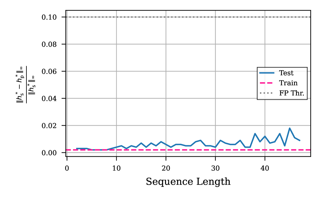
Figure 5: The difference between the fixed-point computed sequentially (i.e., computing the fixed-point for each token separately) and the fixed-point computed in parallel (i.e., computed through (11)) on the $A_{5}$ task trained on sequence length $16$ to convergence. The x-axis denotes the test sequence length, and the y-axis the normalized difference. The dashed gray line denotes the threshold for stopping the fixed-point iterations.

The dense matrix $\mathbf{A}_{t}$ of the corresponding dense RNN in 1 at the fixed-point $h^{*}$ now also depends on the hidden state $h_{t-1}^{*}$, akin to traditional RNNs. This means that the fixed-point iteration is no longer-convex and a solution $h^{*}$ may not be unique. Therefore different fixed-point methods are not guaranteed to converge to the same result. In particular, fixed-points found in parallel (or chunked) form at training time or sequentially at inference time could not be equivalent anymore. While we observe that this is indeed the case at initialization, during training the two methods of finding fixed-points become gradually closer until they produce the same value when the model is fully trained. We provide empirical evidence for this claim in Appendix, Figure 5.

4.4 Dependence on $h_{t-1}$ in theory

We hypothesize that the dependence of the matrices $\lambda_{t}$, $\mathbf{B}_{t}$, $\mathbf{C}_{t}$, and $\mathbf{Q}_{t}$ may provide a mechanism for the model to retain and manipulate positional information over the sequence. Jelassi et al. (2024) and Trockman et al. (2024) show that position embeddings could play a crucial role in copy tasks by acting similar to hashing keys in a hashing table. We extend their mechanistic approach to understand why two-layers of linear attention could need $h_{t-1}^{\ell-1}$ to generate appropriate position embeddings for the hashing mechanism.

Specifically consider $y_{t}=\mathbf{C}_{t}^{\top}h_{t}$ with $h_{t}=h_{t-1}+\mathbf{B}_{t}x_{t}^{\top}$, assuming that a linear RNN with matrix-state can express linear attention by setting $\lambda_{t}\approx\mathbf{1}~\forall t$. Upon receiving an input sequence $\{x_{1},x_{2},\dots,x_{\delta}\}$ of length $\delta$ followed by a delimiter element $x_{\mathbf{s}}$, the model is expected to copy the input sequence autoregressively, i.e. to start producing $\{x_{1},x_{2},\dots,x_{\delta}\}$ at output positions $\delta+1$ to $2\delta$. Following (Arora et al., 2024), the second layer could use position embeddings as hashing keys to detect and copy each token. More concretely, if the first layer receives a sequence $\{x_{1},x_{2},\dots,x_{\delta},x_{\mathbf{s}},x_{1},x_{2},\dots,x_{\delta-1}\}$ of size $2\delta$ and augments it with shifted position embeddings $\{p_{i}\}_{i=1}^{\delta}$ to produce the hidden sequence $\{x_{1}+p_{1},x_{2}+p_{2},\dots,x_{\delta}+p_{\delta},x_{\mathbf{s}}+p_{1},x_{1}+p_{2},\dots,x_{\delta-1}+p_{\delta}\}$, then a second layer can act as a linear transformer and produce the sequence $\{x_{1},x_{2},\dots,x_{\delta}\}$ at output positions $\delta+1$ to $2\delta$. In the following, we focus on the conditions for the first layer to produce the shifted position embeddings.

We start by assuming that the first layer has a skip-connection $y_{t}^{\top}=\mathbf{C}_{t}^{\top}h_{t}+x_{t}^{\top}$. In this case, the inputs can be augmented if the recurrence is able to produce shifted encodings $p_{t-\delta}=p_{t}$ for $\delta<t$ using $p_{t}^{\top}=\mathbf{C}_{t}^{\top}h_{t}$. This condition can be unrolled as

$$\mathbf{C}_{t-\delta}^{\top}h_{t-\delta}\overset{!}{=}\mathbf{C}_{t}^{\top}h_{t-\delta}+\mathbf{C}_{t}^{\top}\sum_{\smash{\tau=t-\delta+1}}^{t}\mathbf{B}_{\tau}x_{\tau}^{\top} \forall\delta<t.$$

and is satisfied if the equations $\mathbf{C}_{t-\delta}^{\top}h_{t-\delta}\overset{!}{=}\mathbf{C}_{t}^{\top}h_{t-\delta}$ and

$$\mathbf{C}_{t}^{\top}\sum_{\tau=t-\delta+1}^{t-1}\mathbf{B}_{\tau}x_{\tau}^{\top}\overset{!}{=}-\mathbf{C}_{t}^{\top}\mathbf{B}_{t}x_{t}^{\top}$$

hold. Such conditions could only be true if $\mathbf{B}_{t}$ and $\mathbf{C}_{t}$ are a function of the previous hidden state $h_{t-1}$ because they need to be able to retain information about $\{x_{i}\}_{i=t-\delta+1}^{t-1}$. While not an explicit mechanism for copying, this derivation provides insight into why a dependency on $h_{t-1}$ could be helpful.

4.5 Expressing linear attention with $\lambda_{t}\approx\mathbf{1}~\forall t$

Recent parameterizations of transition matrices $\lambda_{t}$ use the exponential of a negative number as opposed to the sigmoid function due to the saturation of the sigmoid (Gu et al., 2022). However, this parameterization still does not provide a mechanism to express linear attention with $\lambda_{t}\approx\mathbf{1}$ in a controlled way. To that end, De et al. (2024) propose to separate the lower-bound of $\lambda_{t}$ from its selective component $\Delta_{t}$ by setting $\lambda_{t}=\exp\left(-c\cdot\text{softplus}\left(\omega\right)\cdot\Delta_{t}\right)$. With a selective parameter $0\preceq\Delta_{t}\preceq\mathbf{1}$, an input independent component $\omega$, a temperature $c$, and the softplus function, the transition matrix $\lambda_{t}$ obeys the lower-bound $\lambda_{t}\succeq\exp\left(-c\cdot\text{softplus}\left(\omega\right)\right)$. While the selective component $\Delta_{t}$ seems to be a crucial element for certain tasks in a linear RNN (Gu & Dao, 2023), we believe it also introduces a recency bias to the recurrence. We present the following theorem as evidence for this claim.

Theorem 4.1.

Let $h_{t}=\lambda_{t}\cdot h_{t-1}+x_{t}$ define a 1-dimensional RNN parameterized by $\omega,b$ as $\lambda_{t}=\omega^{\top}x_{t}+b$. Let the input $x_{t}\sim\mathcal{N}\left(0,1\right)$, the bias term positive, and the gate be parameterized as $\lambda_{t}=\sigma\left(\omega^{\top}x_{t}+b\right)$. We define the expected memory of the RNN model $\mathcal{M}\left(\omega,b\right)$ as the expected length of sequence $\mathcal{T}$ in which we have $\lambda_{t}>0.99$ for $t\in(0,\mathcal{T}]$. Then we have: $\mathcal{M}\left(\omega,b\right)\propto\exp\left(\|\omega\|^{2}_{2}\right)^{-1}$. Proof in App. C.

Theorem 4.1 shows an exponential decrease in memory capacity as the selective component $\Delta_{t}$ becomes more prominent. This means that the weights mapping an input $x_{t}$ to $\Delta_{t}$ need to be initialized to $0$ in order facilitate $\lambda_{t}\approx\mathbf{1}~\forall t$. In that way, the model avoids the recency bias linked to selectivity and empirically improves the performance on the copy task.

5 The Bedouin

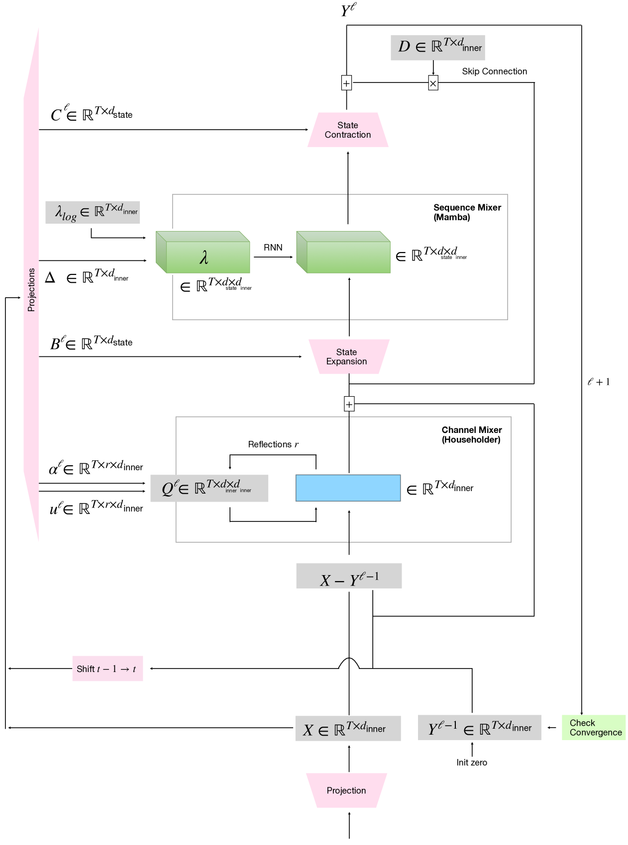
Figure 6: Sketch of our Beduin architecture

In this section, we combine the findings from the previous sections into a dense variant of Mamba (Gu & Dao, 2023). After a short recap of Mamba, we introduce the fixed-point iteration and parametrization of our new model which we call The Bedouin. A diagram is available in Appendix, Figure 6.

5.1 Mamba: Selective SSMs

Mamba is a multi-layer network, with an embedding size of $d_{\text{model}}$. A Mamba block is a matrix state diagonal linear RNN which first expands a sequence of embeddings by a factor of $e$ to size $d_{\text{inner}}=e\times d_{\text{model}}$, and then computes an element-wise recurrence on the matrix hidden states $h_{t}\in\mathbb{R}^{d_{\text{state}}\times d_{\text{inner}}}$ as

$$h_{t}=\lambda_{t}\odot h_{t-1}+\mathbf{B}_{t}\left(\Delta_{t}x_{t}\right)^{\top},$$ (10)

where $\lambda_{t}\in\mathbb{R}^{d_{\text{state}}\times d_{\text{inner}}}$ is an input-dependent state transition vector, $\mathbf{B}_{t}\in\mathbb{R}^{d_{\text{state}}}$ an input transition vector, $x_{t}\in\mathbb{R}^{d_{\text{inner}}}$ the input, and $\Delta_{t}\in\mathbb{R}^{d_{\text{inner}}\times d_{\text{inner}}}$ a diagonal matrix which acts an input normalization term. The matrices are parameterized as:

$$\lambda_{t} =\exp\left(-\lambda_{\log}\Delta_{t}\right), \lambda_{\log} =\exp\left(\omega\right),$$

$$\Delta_{t} =\text{diag}\left(\text{softplus}\left(\mathbf{W}_{\Delta}x_{t}+b_{\Delta}\right)\right), \mathbf{B}_{t} =\mathbf{W}_{\mathbf{B}}x_{t},$$

with $\omega\in\mathbb{R}^{d_{\text{state}}\times d_{\text{inner}}}$, $\mathbf{W}_{\Delta}\in\mathbb{R}^{d_{\text{inner}}\times d_{\text{inner}}}$, $\mathbf{W}_{\mathbf{B}}\in\mathbb{R}^{d_{\text{state}}\times d_{\text{inner}}}$, and $b_{\Delta}\in\mathbb{R}^{d_{\text{inner}}}$. The output of a Mamba block $y_{t}\in\mathbb{R}^{d_{\text{inner}}}$ is a contraction of the matrix hidden state with $\mathbf{C}_{t}\in\mathbb{R}^{d_{\text{state}}}$

$$y_{t}^{\top}=\mathbf{C}_{t}^{\top}h_{t},\quad\mathbf{C}_{t}=\mathbf{W}_{\mathbf{C}}x_{t},$$

for $\mathbf{W}_{\mathbf{C}}\in\mathbb{R}^{d_{\text{state}}\times d_{\text{inner}}}$. Note that Mamba proposes a skip connection of $y_{t}+\mathbf{D}\odot x_{t}$, where $\mathbf{D}\in\mathbb{R}^{d_{\text{inner}}}$ is an input-independent vector. Finally, the model output is usually scaled by a gated linear unit (GLU) as $\tilde{y}_{t}=\mathbf{G}_{t}\odot y_{t}$, where $\mathbf{G}_{t}=\text{SiLU}\left(\mathbf{W}_{G}x_{t}\right)$ is a non-linear function of the input.

5.2 The Bedouin iteration

Let us introduce the fixed-point iteration to the Mamba architecture. We represent the hidden state as $h_{t}^{\ell}$, where $t$ is the token index (i.e., indexing over the sequence dimension), and $\ell$ corresponds to the fixed-point iteration index (i.e., indexing over the depth dimension). The same notation is used for other variables to emphasize when they depend on the input and hidden state of the current iteration. We propose the following iteration to adapt Mamba (10) to the fixed-point mechanism for matrix state RNNs (9):

In order to limit the Lipschitz constant according to Theorem 3.2, we use L2 normalized $\mathbf{\bar{B}}_{t}^{\ell}$ and $\mathbf{\bar{C}}_{t}^{\ell}$. Furthermore, we replace the normalization term $(\mathbf{1}-\lambda_{t})$ with $\Delta_{t}$ to stay compatible with the Mamba implementation. Expanding $y_{t}^{\ell-1}$ yields the recurrence on the matrix state

$$h_{t}^{\ell}=\lambda_{t}\odot h_{t-1}^{\ell}+\text{const}+\mathbf{\bar{B}}_{t}^{\ell}(\mathbf{\bar{C}}_{t}^{\ell-1})^{\top}h_{t}^{\ell-1}(\mathbf{I}-\mathbf{Q}_{t}^{\ell})^{\top}\Delta_{t},$$

where the last term nicely illustrates the two components which mix the channels of the hidden states: the low-rank matrix $\mathbf{\bar{B}}_{t}^{\ell}(\mathbf{\bar{C}}_{t}^{\ell-1})^{\top}$ mixes over the dimension $d_{\text{state}}$, while $(\mathbf{I}-\mathbf{Q}_{t}^{\ell})^{\top}$ mixes over the dimension $d_{\text{inner}}$. This factorization significantly simplifies the fourth-order tensor mixer formulation introduced in (8) and performs well in practice.

Finally, Bedouin (11) can be expressed as Mamba (10)

$$h_{t}^{\ell}=\lambda_{t}\odot h_{t-1}^{\ell}+\mathbf{\bar{B}}_{t}^{\ell}\left(\Delta_{t}\tilde{x}_{t}^{\ell}\right)^{\top},$$ (12)

with an adjusted input $\tilde{x}_{t}^{\ell}=\mathbf{Q}_{t}^{\ell}\left(x_{t}-y_{t}^{\ell-1}\right)+y_{t}^{\ell-1}$. In other words, one fixed-point step consists of a channel mixing using $\mathbf{Q}_{t}$, followed by a sequence mixing using Mamba. This separation of concerns allows to speed up the parallel recurrence in time using the Mamba implementation. To find a fixed-point, the two phases are repeated until convergence, i.e. $\frac{\|y^{\ell}-y^{\ell-1}\|_{\infty}}{\|y^{\ell}\|_{\infty}}<0.1$. For a visual summary of the complete fixed-point iteration, please refer to Appendix, Figure 6.

After convergence to a fixed-point, $h_{t}^{*}$ and $y_{t}^{*}$ present the hidden state and output of the dense matrix-valued RNN. Similar to Mamba, we apply a gated linear unit to the output

$$\tilde{y}_{t}^{*}=\mathbf{G}_{t}\odot\text{SiLU}\left(y_{t}^{*}\right)$$

using $\mathbf{G}_{t}\in\mathbb{R}^{d_{\text{inner}}}$ and the SiLU activation function.

5.3 Parameterization

Following the analyses in Sec. 4, we propose some changes to the input-dependent parameters. Specifically, we adopt the definition of $\lambda_{t}$ from Griffin (De et al., 2024)

$$\lambda_{t} =\exp\left(-c\cdot\lambda_{\text{log}}\cdot\Delta_{t}\right), \lambda_{\text{log}} =\text{softplus}\left(\omega\right),$$

$$\Delta_{t} =\text{diag}\left(\sigma\left(\mathbf{W}_{\Delta}^{x}x_{t}+b_{\Delta}\right)\right), \mathbf{B}_{t}^{\ell} =\mathbf{W}_{\mathbf{B}}^{x}x_{t}+\mathbf{W}_{\mathbf{B}}^{y}y_{t-1}^{\ell-1},$$

with their proposed hyperparameter choice $c=8$, and model the dependence on the previous output with $\mathbf{C}_{t}^{\ell}=\mathbf{W}_{\mathbf{C}}^{x}x_{t}+\mathbf{W}_{\mathbf{C}}^{y}y_{t-1}^{\ell-1}$ and $\mathbf{G}_{t}=\mathbf{W}_{\mathbf{G}}^{x}x_{t}+\mathbf{W}_{\mathbf{G}}^{y}y_{t-1}^{*}$, respectively. Finally, we keep the skip connection in Mamba, but remove the short convolution due to the previous state dependency.

For the channel mixer $\mathbf{Q}_{t}^{\ell}$, we use the formulation based on the product of generalized Householder matrices and parameterize the $i=1,\ldots,r$ reflections in (6) with

$$~\mathbf{u}_{it}^{\ell} =\mathbf{W}_{\mathbf{u}_{i}}^{x}x_{t}+\mathbf{W}_{\mathbf{u}_{i}}^{y}y_{t-1}^{\ell-1},\qquad\mathbf{\bar{u}}_{it}^{\ell}=\frac{\mathbf{u}_{it}^{\ell}}{\left\|\mathbf{u}_{it}^{\ell}\right\|_{2}},$$

$$~\alpha_{it}^{\ell} =\sigma\left(\left(\textbf{w}_{\alpha_{i}}^{x}\right)^{\top}x_{t}+\left(\textbf{w}_{\alpha_{i}}^{y}\right)^{\top}y_{t-1}^{\ell-1}\right).$$

6 Evaluation

In this section, we provide experimental results for our proposed model. For a detailed summary of the experiment setup, please refer to App. E.

State Tracking

The task of tracking state in the alternating group on five elements ($A_{5}$) is one of the tasks introduced in (Merrill et al., 2024) to show that linear RNNs and SSMs cannot solve state-tracking problems. $A_{5}$ is the simplest subset of $S_{5}$, the word problem involving tracking the permutation of five elements. In these tasks, a model is presented with an initial state and a sequence of permutations. As the output, the model is expected to predict the state that results from applying the permutations to the initial state. Solving these task with an RNN requires either a dense transition matrix or the presence of non-linearity in the recurrence. It is therefore a good proxy to verify the state-tracking ability of Bedouin. In order to investigate the out-of-distribution generalization ability of the model, we train the model with a smaller train sequence length and evaluate for larger (more than $\times 3$) sequence lengths.

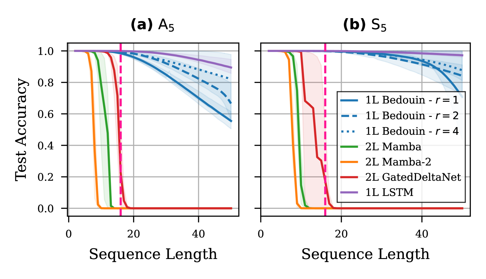
Figure 3: Sequence length generalization on (a) $A_{5}$ and (b) $S_{5}$. We compare a 1-layer Bedouin with a mixer $\mathbf{Q}_{t}$ of $r$ reflections to baselines with $L$ layers. The pink line denotes the train sequence length.

Copying

We use the copy task (Jelassi et al., 2024) in order to assess the memory capabilities of Bedouin. In this task, the model is presented with a fixed-size sequence of elements, and expected to copy a subsequence of it after receiving a special token signaling the start of the copying process. In order to investigate the out-of-distribution generalization ability of the model, we train the models with sequence length $<50$, and assess the x2 length generalization following Jelassi et al. (2024) and Trockman et al. (2024).

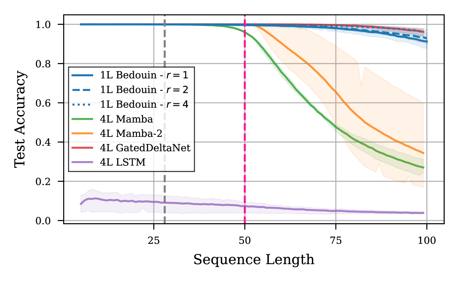
Figure 4: Sequence length generalization on the copy task. We compare a 1-layer Bedouin with a mixer $\mathbf{Q}_{t}$ of $r$ reflections to baselines with $L$ layers. The gray vertical line denotes the median number of fixed-point iterations at test time. The pink line denotes the maximum train sequence length.

The Chomsky Hierarchy

Following Grazzi et al. (2024), we also evaluate Bedouin on the remaining unsolved task of the Chomsky Hierarchy of language problems introduced by Beck et al. (2024). Specifically, we focus on the mod arithmetic task with brackets, for which the best performance reported so far according to Grazzi et al. (2024) is an accuracy of $0.2$. Following the setup of Grazzi et al. (2024), we train on sequence lengths $3$ to $40$ and report scaled accuracies on test sequences of lengths $40$ to $256$. For Bedouin, we use a $2$-layer model with $r=4$ reflections, i.e. the best performing model in the $A_{5}$ experiment.

Model	Accuracy
2L Transformer	0.025
2L mLSTM	0.034
2L sLSTM	0.173
2L Mamba	0.136
2L DeltaNet	0.200
2L Bedouin ($r=4$)	0.280

Table 2: The accuracy of various models on modular arithmetic with brackets. We adopt the reported numbers in (Grazzi et al., 2024) evaluating baselines the extended $[-1,1]$ eigenvalue range. Scores are commonly used scaled accuracies between $1.0$ and $0.0$ (random guessing). Highlighted is the best performance in each category.

6.1 Results

We compare Bedouin on the three tasks introduced above to Mamba (Gu & Dao, 2023), Mamba-2 (Dao & Gu, 2024), Gated DeltaNet (Yang et al., 2025) and the original LSTM (Hochreiter & Schmidhuber, 1997). In order to keep the number of layers at the same order of magnitude, we use two layers (2L) for the diagonal linear RNN baselines and one layer (1L) for Bedouin and LSTM. This keeps the number of parameters for the Bedouin comparable to the baselines (see Figure 2), and smaller than Gated DeltaNet for all experiments. For Bedouin, we report results for $r\in\{1,2,4\}$ Householder reflections of $\mathbf{Q}_{t}$ and a maximum number of $100$ fixed-point iterations. However, we also investigate the effect of limiting the number of fixed-point iterations allowed during training to $\ell_{\text{max}}\in\{2,4,8,16\}$ in Fig. 1. In order to reduce the average number of iterations, we also evaluate a randomization scheme where we sample from the Gamma distribution $\ell_{\text{max}}\sim\Gamma(4,1)$ with mean $4$ and mode $3$.

State Tracking.

In Figure 3, we compare Bedouin for $r\in\{1,2,4\}$ reflections and a maximum number of fixed-point iterations $\ell_{\text{max}}=16$ to the baselines on the $A_{5}$ and $S_{5}$ tasks with sequence length $16$. As expected, the LSTM solves $A_{5}$ and $S_{5}$, while Mamba and Mamba-2 are not able to learn it at the training sequence length.

Copying.

In Figure 4, we evaluate length generalization on the copying task . Both the Mamba and Mamba-2 models struggle with x2 generalization, which proves the effectiveness of our proposed modifications for better memory. The best-performing baseline is Gated DeltaNet, which is specifically designed to do well on the associative recall task (Yang et al., 2025) and is in fact a linear Transformer variant with about $\times 2$ parameters as Bedouin with mixer rank $1$. Note that the number of iterations required by Bedouin to reach the fixed point (gray vertical line) is well below the maximum sequence length of the data.

The Chomsky Hierarchy.

In Table 2, we evaluate modular arithmetic with brackets. We observe that a 2-layer Bedouin outperforms the baselines reported in (Grazzi et al., 2024) with a comparable number of parameters. In Figure 7, we plot the validation accuracy as a function of the number of fixed-point iterations. We observe that the accuracy plateaus at $20$ iterations, which is significantly less than the shortest and longest sequence in the validation set. Therefore, the number of iterations required by the Bedouin to reach its fixed point clearly does not scale with the sequence length in this task.

6.2 Required Number of Fixed-Point Iterations

A fixed-point iteration inevitably introduces sequential overhead to the computation of a model. While this might be acceptable for sequential generation at test time, reduced parallelism can be inhibiting at training time. In Figure 1, we therefore evaluate Bedouin on $A_{5}$ with a limited number of fixed-point iterations at training time $\ell_{\text{max}}$. We observe that the performance decreases once $\ell_{\text{max}}$ is lower than the training sequence length of $16$. Randomly sampling $\ell_{\text{max}}$ during training, however, allows to reduce the average sequential steps to $4$ while maintaining very high sequence length generalization at test time. We want to highlight that as explained in the previous paragraphs, we do not observe this increase in the number of fixed-point iterations in the other tasks.

7 Discussion

A fixed-point mechanism, such as the one introduced in this paper, endows a parallelizable, diagonal linear RNN with the ability to dynamically increase the sequential computation per token and describe a dense linear RNN in the limit. Our results show that such a paradigm can enable both strong state-tracking and memory capabilities with a constant number of parameters in a combined sequence and channel mixing layer (Figure 2). In fact, the fixed-point iteration gradually transforms a diagonal (i.e., channel-wise) RNN into a dense (i.e., channel-mixing) RNN, thereby allowing to trade parallel computation for expressivity (Figure 1).

For Fixed-Point RNNs to become competitive in practice, it is paramount to understand the trade-offs between parallel and sequential computation. In the worst case, if the sequential overhead is linear in the sequence length $T$, the model essentially behaves like a traditional, non-linear RNN with quadratic runtime $O(T^{2})$. This, however, is not necessarily a disadvantage if the model is capable of adapting its sequential steps to the difficulty of the task, with negligible cost for the least demanding tasks. In this paper, we focus on introducing and parameterizing the framework for Fixed-Point RNNs. Therefore, we leave the analysis and improvement of fixed-point convergence speeds beyond our preliminary results (Figure 1, 4, 7) to future work.

Fixed-Point RNNs present an interesting opportunity to be fused into a single GPU kernel with reduced memory I/O. This is an inherent advantage resulting from performing repeated computations on the same operands. However, in order to make the most out of this advantage, we need to consider several open problems: (1) the fixed-point needs to be independent of the level of parallelism used in fixed-point iterations, (2) the parameterization of the model needs to adhere to hardware limitations, (3) a balance between the structure and expressiveness needs to be struck when parameterizing the mixer $\mathbf{Q}_{t}$. Future progress on these problems could enable significant speed-ups in practical implementations of Fixed-Point RNNs.

Conclusion

In this paper, we presented a framework to cast a general class of dense linear RNNs as fixed-points of corresponding diagonal linear RNNs. We then show a seamless adaptation of the proposed Fixed-Point RNN framework into the linear attention family of architectures. The proposed framework provides a mechanism to trade expressivity with computation complexity while uniting the expressivity of recurrent models with the improved memory of linear attention models. Following encouraging results on toy tasks specifically designed to assess these capabilities, we hope this paper enables more expressive sequence mixing models without sacrificing memory capabilities.

Appendix

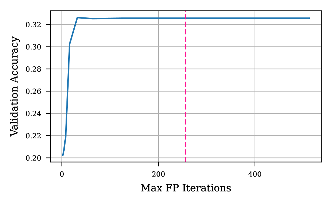
Figure 7: Number of fixed-point iterations on the modular arithmetic task at test time. We report the validation accuracy after convergence for the number of fixed-point iterations caped at various values ranging from $2$ to $512$. The pink dashed line denotes the maximum sequence length during validation.

Appendix A Proof for Theorem 3.2

We start the proof with the unrolled form of the linear RNN

$$f_{\theta}(x,h)_{t}=\sum_{\tau=0}^{t}\Lambda^{t-\tau}\left(\mathbf{I}-\Lambda\right)\left(\mathbf{Q}\mathbf{B}_{\tau}x_{\tau}+\left(\mathbf{I}-\mathbf{Q}\right)h_{\tau}\right).$$

Note that in order to prove the theorem, we need to show that

$$\left\|f_{\theta}(x,h)_{t}-f_{\theta}(x,h^{\prime})_{t}\right\|_{2}<\left\|h-h^{\prime}\right\|_{2},$$

where $h$ and $h^{\prime}$ are two arbitrary hidden states. From the unrolled form, this is equivalent to

$$\left\|\sum_{\tau=0}^{t}\Lambda^{t-\tau}\left(\mathbf{I}-\Lambda\right)\left(\mathbf{I}-\mathbf{Q}\right)(h_{\tau}-h_{\tau}^{\prime})\right\|_{2}<\left\|h-h^{\prime}\right\|_{2}.$$ (13)

From the Cauchy-Schwarz inequality, we can upper-bound the LHS of (13) as

$$\left\|\sum_{\tau=0}^{t}\Lambda^{t-\tau}\left(\mathbf{I}-\Lambda\right)\left(\mathbf{I}-\mathbf{Q}\right)(h_{\tau}-h_{\tau}^{\prime})\right\|_{2}\leq\left\|\sum_{\tau=0}^{t}\Lambda^{t-\tau}\right\|_{2}\cdot\left\|\mathbf{I}-\Lambda\right\|_{2}\cdot\left\|\mathbf{I}-\mathbf{Q}\right\|_{2}\cdot\left\|h_{\leq t}-h_{\leq t}^{\prime}\right\|_{2},$$

where $h_{\leq t}$ corresponds to the concatenation of the hidden states $h_{\tau}$ for $\tau\leq t$. Now to prove this product is $<\left\|h-h^{\prime}\right\|_{2}$, consider the terms individually. Since $\left\|h_{\leq t}-h_{\leq t}^{\prime}\right\|_{2}\leq\left\|h-h^{\prime}\right\|_{2}$, the remaining terms need to be $<1$. Assuming $\Lambda$ is contractive, we use the Neumann series $\sum_{\tau=0}^{t}\Lambda^{t-\tau}\leq\mathbf{I}-\Lambda$ and get

$$\left\|\sum_{\tau=0}^{t}\Lambda^{t-\tau}\right\|_{2}\cdot\left\|\mathbf{I}-\Lambda\right\|_{2}\leq 1.$$

Finally, it remains to show that

$$\left\|\mathbf{I}-\mathbf{Q}\right\|_{2}<1.$$

This condition can be satisfied if $\mathbf{I}-\mathbf{Q}$ is contractive. This completes our proof.∎

Appendix B Proof for Theorem 3.3

We start the proof by setting $\delta:=\frac{\partial\mathcal{L}}{\partial f}$ and $\mathbf{J}_{x}:=\mathbf{J}_{x}(h^{*})$. Then, we can write the backward propagation as $\frac{\partial\mathcal{L}}{\partial x}=\left(\mathbf{J}_{x}^{*}\right)^{\top}\delta$. In order to prove that the gradient computed at the fixed-point is a descent direction, we need to show that $\mathbf{J}_{x}^{\top}\delta$ is in the direction of $\left(\mathbf{J}_{x}^{*}\right)^{\top}\delta$, or in other words, we have $\delta^{\top}\mathbf{J}_{x}^{*}\mathbf{J}_{x}^{\top}\delta\geq 0$. This is equivalent to showing that the symmetric part of the matrix $\mathbf{J}_{x}^{*}\mathbf{J}_{x}^{\top}$ is positive semi-definite.

Now note that from (5) we have: $\mathbf{J}_{x}^{*}\mathbf{J}_{x}^{\top}=\left(\mathbf{I}-\mathbf{J}_{h}\right)^{-1}\mathbf{J}_{x}\mathbf{J}_{x}^{\top}$. From our assumption $\mathbf{J}_{x}=\mathbf{J}_{h}:=\mathbf{J}$, we need to show that the symmetric part of the matrix $\left(\mathbf{I}-\mathbf{J}\right)^{-1}\mathbf{J}\mathbf{J}^{\top}$ is positive semi-definite. Note that using the Neumann series, we can write:

$$\left(\mathbf{I}-\mathbf{J}\right)^{-1}\mathbf{J}=\sum_{i=1}^{\infty}\mathbf{J}^{i}=\mathbf{J}\sum_{i=0}^{\infty}\mathbf{J}^{i}=\mathbf{J}\left(\mathbf{I}-\mathbf{J}\right)^{-1}.$$

Therefore, we have $\left(\mathbf{I}-\mathbf{J}\right)^{-1}\mathbf{J}\mathbf{J}^{\top}=\mathbf{J}\left(\mathbf{I}-\mathbf{J}\right)^{-1}\mathbf{J}^{\top}$. Going back to the definition of positive semi-definiteness, we need to show that $\delta^{\top}\mathbf{J}\left(\mathbf{I}-\mathbf{J}\right)^{-1}\mathbf{J}^{\top}\delta>0$ for all $\delta$. Setting $\omega=\mathbf{J}^{\top}\delta$, this is equivalent to having $\omega^{\top}\left(\mathbf{I}-\mathbf{J}\right)^{-1}\omega$. Note that from our assumption for the Lipschitz constant of the function, we have $\left\|\mathbf{J}\right\|_{2}<1$, which means $\left(\mathbf{I}-\mathbf{J}\right)$ has strictly positive eigenvalues. This completes our proof.∎

Appendix C Proof for Theorem 4.1

Note that we can write $\mathcal{M}\left(\omega,b\right)$ as $\mathcal{M}\left(\omega,b\right)=\text{Prob}\left(\omega^{\top}x+b\leq\sigma^{-1}(0.99)\right)^{-1}.$ Given the distribution of $x$, we can write $\text{Prob}\left(\omega^{\top}x+b\leq\sigma^{-1}(0.99)\right)=\Phi\left(\frac{\sigma^{-1}(0.99)-b}{\|\omega\|_{2}^{2}}\right)$. Given that $\Phi(\cdot)$ can be written as the integration of a quadratic exponential function w.r.t. the denominator of its argument, this completes our proof.∎

Appendix D Low-Rank Expressiveness

In this section, we prove that SSMs with low-rank structure can be maximally expressive under weak assumptions on the growth of the rank with hidden dimension. To do this we first place ourselves in the general setting of (Cirone et al., 2024b), accordingly we consider models given by controlled differential equations of type:

$$\mathrm{d}Y_{s}=\sum_{i=1}^{d_{\omega}}A^{i}Y_{s}\text{d}\omega^{i}_{s},\quad Y_{0}\in\mathbb{R}^{d_{Y}}$$ (14)

Following the notation and methodology of (Cirone et al., 2024b)[B.4] ), this can be written in terms of the Signature as

$$\mathbf{Y}((A^{i})_{i},Y_{0},\omega)_{t}:=Y_{t}=\sum_{I\in\mathbb{W}_{d_{\omega}}}(A^{I}Y_{0})~S^{I}(\omega)_{[0,t]}$$ (15)

where $\mathbb{W}_{d_{\omega}}$ is the set of words in the alphabet $[[d_{\omega}]]:=\{1,\dots,d_{\omega}\}~$ (i.e. $\mathbb{W}_{d_{\omega}}=\bigcup_{n\geq 0}[[d_{\omega}]]^{n}$ ) and for a given word $I=i_{1}\dots i_{n}$ with $S^{I}(\omega)_{[0,t]}$ we refer to the $I$th component of the signature tensor $S(\omega)_{[0,t]}$ i.e.

$$S^{I}(\omega)_{[0,t]}=\underbrace{\int\cdots\int}_{\begin{subarray}{c}u_{1}<\cdots<u_{n}\\ u_{i}\in[0,t]\end{subarray}}\text{d}\omega^{i_{1}}_{u_{1}}\cdots\text{d}\omega^{i_{n}}_{u_{n}}.$$

It follows directly from (15) that any linear readout of $Y_{t}$ can be represented as a series in signature terms. As a result, these systems are fundamentally restricted to learning functions that closely approximate these convergent series.

Maximal expressivity is attained when any finite linear combination of signature terms can be approximated by a linear readout on $Y_{t}$ via suitable configurations of the matrices $A^{i}$.

Definition D.1.

Fix a set of paths $\mathcal{X}\subseteq C^{1-var}([0,1];\mathbb{R}^{d})$. We say that a sequence $(\mathcal{A}_{N},\mathcal{Y}_{N})_{N\in\mathbb{N}}$, where $\mathcal{Y}_{N}\subseteq\mathbb{R}^{N}$ and $\mathcal{A}_{N}\subseteq\mathbb{R}^{N\times N}$, achieves maximal expressivity for $\mathcal{X}$ whenever for any positive tolerance $\epsilon>0$ and any finite linear combination coefficients $\alpha\in T(\mathbb{R}^{d})$ there exist a choice of parameters $v,(A^{i}),Y_{0}$ in some $\mathbb{R}^{N},\mathcal{A}_{N},\mathcal{Y}_{N}$ in the sequence such that $v^{\top}\mathbf{Y}((A^{i}),Y_{0},\omega)_{\cdot}$ is uniformly close to $\langle\alpha,S(\omega)_{[0,\cdot]}\rangle$ up to an error of $\epsilon$ i.e.

$$\forall\epsilon>0,~\forall\alpha\in T(\mathbb{R}^{d}),~\exists N\geq 0,~\exists(v,(A^{i}),Y_{0})\in\mathbb{R}^{N}\times\mathcal{A}_{N}^{d}\times\mathcal{Y}_{N}~\text{s.t.}$$

$$\sup_{(\omega,t)\in\mathcal{X}\times[0,1]}|\langle\alpha,S(\omega)_{[0,t]}\rangle-v^{\top}\mathbf{Y}((A^{i}),Y_{0},\omega)_{t}|<\epsilon$$

If we are given a sequence of probabilities $\mathbb{P}_{N}$ on $\mathcal{A}_{N}^{d}\times\mathcal{Y}_{N}$ such that $\forall\epsilon>0,~\forall\alpha\in T(\mathbb{R}^{d})$ it holds that

$$\lim\limits_{N\to\infty}\mathbb{P}_{N}\left\{\exists v\in\mathbb{R}^{N}~\text{s.t.}\sup_{(\omega,t)\in\mathcal{X}\times[0,1]}|\langle\alpha,S(\omega)_{[0,t]}\rangle-v^{\top}\mathbf{Y}((A^{i}),Y_{0},\omega)_{t}|<\epsilon\right\}=1$$ (16)

then we say that $(\mathcal{A}_{N},\mathcal{Y}_{N},\mathbb{P}_{N})_{N\in\mathbb{N}}$ achieves maximal probabilistic expressivity for $\mathcal{X}$.

As discussed in the main body of this work in (Cirone et al., 2024b) the authors prove that $(\mathbb{R}^{N\times N},\mathbb{R}^{N},\mathbb{P}_{N})$, where $\mathbb{P}_{N}$ is a Gaussian measure corresponding to the classical Glorot initialization scheme in deep learning, achieves maximal probabilistic expressivity for compact sets.

Albeit expressiveness is thus maximally attained the resulting matrices $A_{i}$ are almost-surely dense, hence the models are not efficiently implementable. As the next result suggests, a possible alternative is given by low-rank matrices:

Proposition D.2.

The sequence of triplets $(\mathbb{R}^{N\times N},\mathbb{R}^{N},\mathbb{P}_{N})$ where $\mathbb{P}_{N}$ is such that

• the initial value has independent standard Gaussian entries $[Y_{0}]_{\alpha}\overset{\mathrm{iid}}{\sim}\mathcal{N}(0,1)$,

• the weight matrices are distributed as $A^{i}\overset{\mathrm{iid}}{\sim}\frac{1}{\sqrt{Nr_{N}}}WM^{\top}$ with $W$ and $M$ independent $N\times r_{N}$ matrices having entries $[W]_{\alpha,\beta},[M]_{\alpha,\beta}\overset{\mathrm{iid}}{\sim}\mathcal{N}(0,1)$,

• the rank parameter $r_{N}$ satisfies $r_{N}\to\infty$ as $N\to\infty$

achieves maximal probabilistic expressivity for compact sets.

Proof.

Following (Cirone et al., 2024b)[B.3.5] we only need to prove a bound of type

$$\left\lVert\frac{1}{N}\langle A_{I}Y_{0},A_{J}Y_{0}\rangle_{\mathbb{R}^{N}}-\delta_{I,J}\right\rVert_{L^{2}(\mathbb{P}_{N})}\leq(\kappa(|I|+|J|))!!~o(1)$$ (17)

as in the full-rank Gaussian case.

We will place ourselves in the graphical setting of (Cirone et al., 2024a) and leverage the fact that (c.f. (Cirone et al., 2024a)[7.1]) their results and techniques naturally hold for rectangular matrices.

In our setting $\frac{1}{N}\langle A_{I}Y_{0},A_{J}Y_{0}\rangle_{\mathbb{R}^{N}}$ corresponds to a product graph $G_{I,J}$ corresponding to a ladder having $2|I|+2|J|$ edges as shown in figure 8. We can then use (Cirone et al., 2024a)[Prop. 2] to compute the square of the $L^{2}$ norm in equation (17), the only difference from the dense case is that half of the vertices (excluding the "middle" one) correspond to a space of dimension $r_{N}$ while the rest to the standard $N$.

Since $r_{N}\to\infty$ and given the scaling $N^{-1}\bigl{(}Nr_{N}\bigr{)}^{-\frac{|I|+|J|}{2}}$, the admissible pairings of $G_{I,J}$ not of order $o(1)$ are only the leading ones. These correspond to product graphs with $\frac{|I|+|J|}{2}$ $r_{N}$-dimensional vertices and $\frac{|I|+|J|}{2}+1$ $N$-dimensional vertices. By the same reasoning as in the full-rank case, these are found to be just the identity pairings.

Moreover, all pairings of $G_{I,J}\sqcup G_{I,J}$ that do not result in an identity pairing in at least one of the two copies are $\mathcal{O}\bigl{(}\frac{1}{N\wedge r_{N}}\bigr{)}$ ( instead of $\mathcal{O}\bigl{(}\frac{1}{N}\bigr{)}$ ). This follows as in the full-rank case.

Since the total number of admissible pairings of $G_{I,J}\sqcup G_{I,J}$ is $\bigl{(}4(|I|+|J|)\bigr{)}!!$, we conclude that equation (17) holds with $\kappa=4$ and $o(1):=\mathcal{O}\bigl{(}\frac{1}{\sqrt{N\wedge r_{N}}}\bigr{)}$.

∎

Figure 8: The product graph $G_{I,J}$ for $I=i_{1}i_{2}i_{3}$ and $J=j_{1}$.

Remark D.3.

Following (Cirone et al., 2024a)[6.1] it's possible to prove that the $W$ and $M$ can be taken as having iid entries from a centred, symmetric but heavy tailed distribution given finiteness of even moments. This distributional choice comes useful in controlling the eigenvalues of $A=WM^{\top}$.

Remark D.4.

While the proof crucially uses the assumption $r_{N}\to\infty$ as $N\to\infty$, at the same time we have not provided an argument against $r_{N}$ not diverging. In figure 9 we present a counterexample, showing that if $r_{N}$ does not diverge then the asymptotics differ from the dense ones, in particular some symmetries are "lost", impossible to recover due to unavoidable noise.

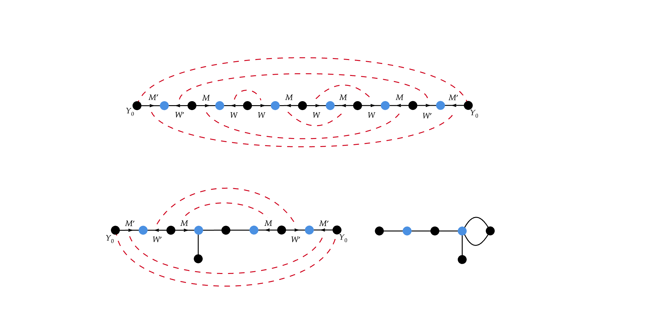
Figure 9: Admissible pairing different from the "identity" paring, but still leading to maximal asymptotic scaling in the bounded $r_{N}$ case. Here, $I=12\neq 1112=J$, and we have highlighted in blue the vertices corresponding to the bounded dimension $r_{N}$. Recall that edges without arrows correspond to the matrix $\mathbf{I}$ (matrix of ones), and that two edges corresponding to matrices $A$ and $B$ which share direction and terminal vertices can be merged into the edge $A\odot B$.

Appendix E Experiment setup

In this section, we will provide our experiment setup for the state tracking, copying, and mod arithmetic tasks.

State tracking.

We train all models for $5$ epochs, with a batch size of $128$, $3$ different random seeds, learning rate set to $0.0001$, weight decay set to $0.01$, gradient clipping 1.0, and the AdamW optimizer (Loshchilov & Hutter, 2017). We sample $1.6$M samples from all the possible permutations, and split the data with a ratio of 4 to 1. We use the implementation and the hyperparameters provided by Merrill et al. (2024). We train the model for sequence length $16$, and evaluate for sequence length $2$ through $50$.

Copying.

We train all models for $10000$ iterations, batch size $128$, $3$ different random seeds, learning rate $0.00001$, weight decay $0.1$, gradient clipping $1.0$, the AdamW optimizer, and with linear learning rate decay after a $300$ iterations warmup. The data is sampled randomly at the start of the training/evaluation. We use a vocab size of $29$, a context length of $256$, and train the model for copy sequence length in the range $5$ to $50$, and evaluate for the range $5$ to $100$. we use the implementation and the hyperparameters provided by Jelassi et al. (2024).

Mod arithmetic.

Our models are trained for $100000$ iterations, batch size $256$, learning rate $0.001$, weight decay $0.1$, and no gradient clipping. The learning rate is decayed using a cosine scheduling by a factor of $0.001$ after $10000$ iterations of warmup. The data is randomly sampled at the start of training/evaluation. We use a vocab size of $12$, with context length $256$, and train data sequence length in the range $3$ to $40$, and the test/evaluation data in the range $40$ to $256$. We use the implementation and the hyperparameters provided by Beck et al. (2024) and Grazzi et al. (2024), which are the same hyperparameters used for training and evaluating the baselines.

References

- Arora et al. (2024) Arora, S., Eyuboglu, S., Zhang, M., Timalsina, A., Alberti, S., Zou, J., Rudra, A., and Ré, C. Simple linear attention language models balance the recall-throughput tradeoff. In Forty-first International Conference on Machine Learning, ICML 2024, Vienna, Austria, July 21-27, 2024. OpenReview.net, 2024.
- Bai et al. (2019) Bai, S., Kolter, J. Z., and Koltun, V. Deep equilibrium models. In Wallach, H. M., Larochelle, H., Beygelzimer, A., d'AlcheBuc, F., Fox, E. B., and Garnett, R. (eds.), Advances in Neural Information Processing Systems, pp. 688–699, 2019.
- Bai et al. (2021) Bai, S., Koltun, V., and Kolter, J. Z. Stabilizing equilibrium models by jacobian regularization. In Meila, M. and Zhang, T. (eds.), Proceedings of the 38th International Conference on Machine Learning, ICML 2021, 18-24 July 2021, Virtual Event, volume 139 of Proceedings of Machine Learning Research, pp. 554–565. PMLR, 2021.
- Banach (1922) Banach, S. Sur les opérations dans les ensembles abstraits et leur application aux équations intégrales. Fundamenta mathematicae, 3(1):133–181, 1922.
- Beck et al. (2024) Beck, M., Pöppel, K., Spanring, M., Auer, A., Prudnikova, O., Kopp, M., Klambauer, G., Brandstetter, J., and Hochreiter, S. xlstm: Extended long short-term memory. In Globersons, A., Mackey, L., Belgrave, D., Fan, A., Paquet, U., Tomczak, J. M., and Zhang, C. (eds.), Advances in Neural Information Processing Systems 38: Annual Conference on Neural Information Processing Systems 2024, NeurIPS 2024, Vancouver, BC, Canada, December 10 - 15, 2024, 2024.
- Broyden (1965) Broyden, C. G. A class of methods for solving nonlinear simultaneous equations. Mathematics of computation, 19(92):577–593, 1965.
- Chen et al. (2021) Chen, Y., Zeng, Q., Ji, H., and Yang, Y. Skyformer: Remodel self-attention with Gaussian kernel and Nystrom method. Advances in Neural Information Processing Systems, 2021.
- Choromanski et al. (2020) Choromanski, K. M., Likhosherstov, V., Dohan, D., Song, X., Gane, A., Sarlos, T., Hawkins, P., Davis, J. Q., Mohiuddin, A., Kaiser, L., et al. Rethinking attention with performers. In International Conference on Learning Representations, 2020.
- Cirone et al. (2024a) Cirone, N. M., Hamdan, J., and Salvi, C. Graph expansions of deep neural networks and their universal scaling limits, 2024a.
- Cirone et al. (2024b) Cirone, N. M., Orvieto, A., Walker, B., Salvi, C., and Lyons, T. J. Theoretical foundations of deep selective state-space models. CoRR, abs/2402.19047, 2024b. doi: 10.48550/ARXIV.2402.19047.
- Dao & Gu (2024) Dao, T. and Gu, A. Transformers are ssms: Generalized models and efficient algorithms through structured state space duality. In Forty-first International Conference on Machine Learning, ICML 2024, Vienna, Austria, July 21-27, 2024. OpenReview.net, 2024.
- De et al. (2024) De, S., Smith, S. L., Fernando, A., Botev, A., Muraru, G., Gu, A., Haroun, R., Berrada, L., Chen, Y., Srinivasan, S., Desjardins, G., Doucet, A., Budden, D., Teh, Y. W., Pascanu, R., de Freitas, N., and Gulcehre, C. Griffin: Mixing gated linear recurrences with local attention for efficient language models. CoRR, abs/2402.19427, 2024. doi: 10.48550/ARXIV.2402.19427.
- Dehghani et al. (2019) Dehghani, M., Gouws, S., Vinyals, O., Uszkoreit, J., and Kaiser, L. Universal transformers. In 7th International Conference on Learning Representations, ICLR 2019, New Orleans, LA, USA, May 6-9, 2019. OpenReview.net, 2019.
- Elman (1990) Elman, J. L. Finding structure in time. Cogn. Sci., 14(2):179–211, 1990. doi: 10.1207/S15516709COG1402\_1.
- Fung et al. (2022) Fung, S. W., Heaton, H., Li, Q., McKenzie, D., Osher, S. J., and Yin, W. JFB: jacobian-free backpropagation for implicit networks. In Thirty-Sixth AAAI Conference on Artificial Intelligence, AAAI 2022, Thirty-Fourth Conference on Innovative Applications of Artificial Intelligence, IAAI 2022, The Twelveth Symposium on Educational Advances in Artificial Intelligence, EAAI 2022 Virtual Event, February 22 - March 1, 2022, pp. 6648–6656. AAAI Press, 2022. doi: 10.1609/AAAI.V36I6.20619.
- Ghaoui et al. (2021) Ghaoui, L. E., Gu, F., Travacca, B., Askari, A., and Tsai, A. Y. Implicit deep learning. SIAM J. Math. Data Sci., 3(3):930–958, 2021. doi: 10.1137/20M1358517.
- Giannou et al. (2023) Giannou, A., Rajput, S., Sohn, J., Lee, K., Lee, J. D., and Papailiopoulos, D. Looped transformers as programmable computers. In Krause, A., Brunskill, E., Cho, K., Engelhardt, B., Sabato, S., and Scarlett, J. (eds.), International Conference on Machine Learning, ICML 2023, 23-29 July 2023, Honolulu, Hawaii, USA, volume 202 of Proceedings of Machine Learning Research, pp. 11398–11442. PMLR, 2023.
- Goel et al. (2022) Goel, K., Gu, A., Donahue, C., and Ré, C. It's raw! audio generation with state-space models. In Chaudhuri, K., Jegelka, S., Song, L., Szepesvári, C., Niu, G., and Sabato, S. (eds.), International Conference on Machine Learning, ICML 2022, 17-23 July 2022, Baltimore, Maryland, USA, volume 162 of Proceedings of Machine Learning Research, pp. 7616–7633. PMLR, 2022.
- Gonzalez et al. (2024) Gonzalez, X., Warrington, A., Smith, J. T. H., and Linderman, S. W. Towards scalable and stable parallelization of nonlinear rnns. In Globersons, A., Mackey, L., Belgrave, D., Fan, A., Paquet, U., Tomczak, J. M., and Zhang, C. (eds.), Advances in Neural Information Processing Systems 38: Annual Conference on Neural Information Processing Systems 2024, NeurIPS 2024, Vancouver, BC, Canada, December 10 - 15, 2024, 2024.
- Granas et al. (2003) Granas, A., Dugundji, J., et al. Fixed point theory, volume 14. Springer, 2003.
- Graves (2016) Graves, A. Adaptive computation time for recurrent neural networks. CoRR, abs/1603.08983, 2016.
- Grazzi et al. (2024) Grazzi, R., Siems, J., Franke, J. K. H., Zela, A., Hutter, F., and Pontil, M. Unlocking state-tracking in linear rnns through negative eigenvalues. CoRR, abs/2411.12537, 2024. doi: 10.48550/ARXIV.2411.12537.
- Gu & Dao (2023) Gu, A. and Dao, T. Mamba: Linear-time sequence modeling with selective state spaces. CoRR, abs/2312.00752, 2023. doi: 10.48550/ARXIV.2312.00752.
- Gu et al. (2022) Gu, A., Goel, K., and Ré, C. Efficiently modeling long sequences with structured state spaces. In The Tenth International Conference on Learning Representations, ICLR 2022, Virtual Event, April 25-29, 2022. OpenReview.net, 2022.
- Hanson & Raginsky (2020) Hanson, J. and Raginsky, M. Universal simulation of stable dynamical systems by recurrent neural nets. In Learning for Dynamics and Control. PMLR, 2020.
- Hochreiter & Schmidhuber (1997) Hochreiter, S. and Schmidhuber, J. Long short-term memory. Neural Comput., 9(8):1735–1780, 1997. doi: 10.1162/NECO.1997.9.8.1735.
- Hochreiter et al. (2001) Hochreiter, S., Bengio, Y., Frasconi, P., et al. Gradient flow in recurrent nets: the difficulty of learning long-term dependencies. A Field Guide to Dynamical Recurrent Neural Networks, 2001.
- Hopfield (1982) Hopfield, J. J. Neural networks and physical systems with emergent collective computational abilities. Proceedings of the National Academy of Sciences, 79(8):2554–2558, 1982. doi: 10.1073/pnas.79.8.2554.
- Jaeger (2001) Jaeger, H. The "echo state" approach to analysing and training recurrent neural networks-with an erratum note. German National Research Center for Information Technology GMD Technical Report, 2001.
- Jelassi et al. (2024) Jelassi, S., Brandfonbrener, D., Kakade, S. M., and Malach, E. Repeat after me: Transformers are better than state space models at copying. In Forty-first International Conference on Machine Learning, ICML 2024, Vienna, Austria, July 21-27, 2024. OpenReview.net, 2024.
- Katharopoulos et al. (2020) Katharopoulos, A., Vyas, A., Pappas, N., and Fleuret, F. Transformers are rnns: Fast autoregressive transformers with linear attention. In International Conference on Machine Learning. PMLR, 2020.
- Korsky (2019) Korsky, S. A. On the computational power of RNNs. PhD thesis, Massachusetts Institute of Technology, 2019.
- Lim et al. (2024) Lim, Y. H., Zhu, Q., Selfridge, J., and Kasim, M. F. Parallelizing non-linear sequential models over the sequence length. In The Twelfth International Conference on Learning Representations, ICLR 2024, Vienna, Austria, May 7-11, 2024. OpenReview.net, 2024.
- Liu et al. (2024) Liu, Y., Tian, Y., Zhao, Y., Yu, H., Xie, L., Wang, Y., Ye, Q., Jiao, J., and Liu, Y. Vmamba: Visual state space model. In Globersons, A., Mackey, L., Belgrave, D., Fan, A., Paquet, U., Tomczak, J. M., and Zhang, C. (eds.), Advances in Neural Information Processing Systems 38: Annual Conference on Neural Information Processing Systems 2024, NeurIPS 2024, Vancouver, BC, Canada, December 10 - 15, 2024, 2024.
- Loshchilov & Hutter (2017) Loshchilov, I. and Hutter, F. Decoupled weight decay regularization. arXiv preprint arXiv:1711.05101, 2017.
- Martens (2020) Martens, J. New insights and perspectives on the natural gradient method. J. Mach. Learn. Res., 21:146:1–146:76, 2020.
- Martin & Cundy (2018) Martin, E. and Cundy, C. Parallelizing linear recurrent neural nets over sequence length. In 6th International Conference on Learning Representations, ICLR 2018, Vancouver, BC, Canada, April 30 - May 3, 2018, Conference Track Proceedings. OpenReview.net, 2018.
- Merrill & Sabharwal (2023) Merrill, W. and Sabharwal, A. The parallelism tradeoff: Limitations of log-precision transformers. Trans. Assoc. Comput. Linguistics, 11:531–545, 2023. doi: 10.1162/TACL\_A\_00562.
- Merrill et al. (2024) Merrill, W., Petty, J., and Sabharwal, A. The illusion of state in state-space models. In Forty-first International Conference on Machine Learning, ICML 2024, Vienna, Austria, July 21-27, 2024. OpenReview.net, 2024.
- Miyato et al. (2025) Miyato, T., Löwe, S., Geiger, A., and Welling, M. Artificial kuramoto oscillatory neurons. In The Thirteenth International Conference on Learning Representations, 2025.
- Nguyen et al. (2024) Nguyen, E., Poli, M., Durrant, M. G., Kang, B., Katrekar, D., Li, D. B., Bartie, L. J., Thomas, A. W., King, S. H., Brixi, G., et al. Sequence modeling and design from molecular to genome scale with Evo. Science, 2024.
- Pascanu et al. (2013) Pascanu, R., Mikolov, T., and Bengio, Y. On the difficulty of training recurrent neural networks. In International Conference on Machine Learning, 2013.
- Peng et al. (2024) Peng, B., Goldstein, D., Anthony, Q., Albalak, A., Alcaide, E., Biderman, S., Cheah, E., Du, X., Ferdinan, T., Hou, H., et al. Eagle and Finch: RWKV with matrix-valued states and dynamic recurrence. arXiv preprint arXiv:2404.05892, 2024.
- Qin et al. (2024) Qin, Z., Yang, S., Sun, W., Shen, X., Li, D., Sun, W., and Zhong, Y. HGRN2: Gated linear RNNs with state expansion. arXiv preprint arXiv:2404.07904, 2024.
- Rumelhart et al. (1986) Rumelhart, D. E., Smolensky, P., McClelland, J. L., and Hinton, G. Sequential thought processes in pdp models. Parallel Distributed Processing: Explorations in the Microstructures of Cognition, 1986.
- Schlag et al. (2021a) Schlag, I., Irie, K., and Schmidhuber, J. Linear transformers are secretly fast weight programmers. In Meila, M. and Zhang, T. (eds.), Proceedings of the 38th International Conference on Machine Learning, ICML 2021, 18-24 July 2021, Virtual Event, volume 139 of Proceedings of Machine Learning Research, pp. 9355–9366. PMLR, 2021a.
- Schlag et al. (2021b) Schlag, I., Irie, K., and Schmidhuber, J. Linear transformers are secretly fast weight programmers. In International Conference on Machine Learning, 2021b.
- Schwarzschild et al. (2021) Schwarzschild, A., Borgnia, E., Gupta, A., Huang, F., Vishkin, U., Goldblum, M., and Goldstein, T. Can you learn an algorithm? generalizing from easy to hard problems with recurrent networks. In Ranzato, M., Beygelzimer, A., Dauphin, Y. N., Liang, P., and Vaughan, J. W. (eds.), Advances in Neural Information Processing Systems 34: Annual Conference on Neural Information Processing Systems 2021, NeurIPS 2021, December 6-14, 2021, virtual, pp. 6695–6706, 2021.
- Schöne et al. (2025) Schöne, M., Rahmani, B., Kremer, H., Falck, F., Ballani, H., and Gladrow, J. Implicit language models are rnns: Balancing parallelization and expressivity, 2025.
- Siegelmann & Sontag (1992) Siegelmann, H. T. and Sontag, E. D. On the computational power of neural nets. In Proceedings of the fifth Annual Workshop on Computational Learning Theory, 1992.
- Siems et al. (2025) Siems, J., Carstensen, T., Zela, A., Hutter, F., Pontil, M., and Grazzi, R. Deltaproduct: Increasing the expressivity of deltanet through products of householders, 2025.
- Smith et al. (2023) Smith, J. T., Warrington, A., and Linderman, S. Simplified state space layers for sequence modeling. In International Conference on Learning Representations, 2023.
- Sun et al. (2023) Sun, Y., Dong, L., Huang, S., Ma, S., Xia, Y., Xue, J., Wang, J., and Wei, F. Retentive network: A successor to transformer for large language models. arXiv preprint arXiv:2307.08621, 2023.
- Tay et al. (2020) Tay, Y., Dehghani, M., Abnar, S., Shen, Y., Bahri, D., Pham, P., Rao, J., Yang, L., Ruder, S., and Metzler, D. Long range arena: A benchmark for efficient transformers. In International Conference on Learning Representations, 2020.
- Trockman et al. (2024) Trockman, A., Harutyunyan, H., Kolter, J. Z., Kumar, S., and Bhojanapalli, S. Mimetic initialization helps state space models learn to recall. CoRR, abs/2410.11135, 2024. doi: 10.48550/ARXIV.2410.11135.
- Ur´ıas (2010) Urías, J. Householder factorizations of unitary matrices. Journal of mathematical physics, 51(7), 2010.
- Vaswani et al. (2017) Vaswani, A., Shazeer, N., Parmar, N., Uszkoreit, J., Jones, L., Gomez, A. N., Kaiser, L., and Polosukhin, I. Attention is all you need. Advances in Neural Information Processing Systems, 2017.
- Waleffe et al. (2024) Waleffe, R., Byeon, W., Riach, D., Norick, B., Korthikanti, V., Dao, T., Gu, A., Hatamizadeh, A., Singh, S., Narayanan, D., et al. An empirical study of Mamba-based language models. arXiv preprint arXiv:2406.07887, 2024.
- Wang et al. (2020) Wang, S., Li, B. Z., Khabsa, M., Fang, H., and Ma, H. Linformer: Self-attention with linear complexity. arXiv preprint arXiv:2006.04768, 2020.
- Yang et al. (2024a) Yang, S., Wang, B., Shen, Y., Panda, R., and Kim, Y. Gated linear attention transformers with hardware-efficient training. In Forty-first International Conference on Machine Learning, ICML 2024, Vienna, Austria, July 21-27, 2024. OpenReview.net, 2024a.
- Yang et al. (2024b) Yang, S., Wang, B., Zhang, Y., Shen, Y., and Kim, Y. Parallelizing linear transformers with the delta rule over sequence length. CoRR, abs/2406.06484, 2024b. doi: 10.48550/ARXIV.2406.06484.
- Yang et al. (2025) Yang, S., Kautz, J., and Hatamizadeh, A. Gated delta networks: Improving mamba2 with delta rule. In The Thirteenth International Conference on Learning Representations, 2025.
- Zucchet & Orvieto (2024) Zucchet, N. and Orvieto, A. Recurrent neural networks: vanishing and exploding gradients are not the end of the story. Advances in Neural Information Processing Systems, 37:139402–139443, 2024.