diss. eth no. 30705

DESIGN AND ANALYSIS OF AN EXTREME-SCALE,
HIGH-PERFORMANCE, AND MODULAR
AGENT-BASED SIMULATION PLATFORM

A thesis submitted to attain the degree of
doctor of sciences
(Dr. sc. ETH Zurich)

presented by
lukas johannes breitwieser
Diplom-Ingenieur, Graz University of Technology
born on 26.04.1987

accepted on the recommendation of
Prof. Dr. Onur Mutlu, examiner
Dr. Fons Rademakers, co-examiner
Prof. Dr. Can Alkan, co-examiner
Dr. Arnau Montagud, co-examiner
Dr. Mohammad Sadrosadati, co-examiner

2024

Lukas Johannes Breitwieser: Design and Analysis of an Extreme-Scale, High-Performance, and Modular Agent-Based Simulation Platform, © 2024

latest version at: 10.5281/zenodo.14505960

Abstract.1Abstract.1AbstractAbstractAbstract.1

Abstract

Agent-based modeling is an indispensable tool for studying complex systems in biology, medicine, sociology, economics, and other fields. However, existing simulation platforms exhibit two major problems: 1) performance: they do not always take full advantage of modern hardware platforms, which leads to low performance and 2) modularity: they often have a field-specific software design. First, the low performance of many agent-based simulation platforms has at least four undesirable consequences: i) It prevents simulations that can model large numbers of agents or complex agent behaviors, which is necessary in modeling large-scale and complex systems, e.g., in biology and epidemiology. ii) It increases the development time of agent-based simulations, which are performed iteratively, leading to much longer latencies in performing such studies. iii) It limits the capability to explore the parameter space or sensitivity analyses, which may lead to suboptimal or even incomplete simulation results. iv) It increases the monetary cost required for computing power. Second, platforms with an inflexible software design make it challenging to implement use cases in different domains. Modelers who do not find a simulation platform that can be easily extended without modifying the platform’s internals may start developing their own simulation tool to satisfy their modeling needs. This situation not only wastes resources in reimplementing already existing functionality but may also lead to compromises due to the complexity of developing a simulator and the often limited development resources.

This dissertation presents a novel simulation platform called BioDynaMo and its major improvement TeraAgent that alleviate the performance and modularity problems via three major works.

First, we lay the platform’s foundation by carefully defining the abstractions and interfaces, setting up the required software infrastructure, and implementing a multitude of features for agent-based modeling. We demonstrate BioDynaMo’s functionality and modularity with three use cases in neuroscience, epidemiology, and oncology. We validate these models with experimental data or an analytical solution, which also demonstrates the correctness of the BioDynaMo implementation. These models show that in BioDynaMo additional functionality can be added easily, and BioDynaMo’s out-of-the-box features allow for concise model definitions in the range of 128–181 lines of C++ code.

Second, we extend the BioDynaMo platform by performing a rigorous performance analysis of agent-based simulation and identifying three key performance challenges for shared-memory parallelism, for which we present solutions. 1) To maximize parallelization, we present an optimized grid to search for neighbors and parallelize the merging of thread-local results. 2) We reduce the memory access latency with a non-uniform memory access aware agent iterator, agent sorting with a space-filling curve, and a custom heap memory allocator. 3) We present a mechanism to omit the collision force calculation under certain conditions. Our solutions result in a up to three orders of magnitude speedup over the state-of-the-art, and the ability to simulate 1.72 billion agents on a single server.

Third, we introduce a distributed simulation engine called TeraAgent that allows scaling out the computation of one simulation to multiple servers. Distributed execution requires the exchange of agent information between servers. We identify such information exchanges as the key bottleneck that prevents the distributed engine from scaling out efficiently, for which we present two main solutions. 1) We add a tailored serialization mechanism to avoid unnecessary work. 2) We extend the agent serialization mechanism with delta encoding to reduce the amount of data transfer. We choose delta encoding to exploit the iterative nature of agent-based simulations. Our solutions enable TeraAgent to 1) simulate 500 billion agents (a 84$\times$ improvement over the state-of-the-art), 2) scale to 84’096 CPU cores, 3) significantly reduce the simulation time (e.g., TeraAgent simulates an iteration of 800 million agents in $0.6\text{\,}\mathrm{s}$ instead of $5\text{\,}\mathrm{s}$), and 4) significantly increase the visualization performance by 39$\times$.

Since its publication and open source release, researchers have used BioDynaMo to study radiotherapy of lung cancer, vascular tumor growth, invasion of Gliomas into surrounding tissue, the formation of retinal mosaics in the eye, freezing and thawing of cells, neuronal geometries, the formation of the cortical layers in the cerebral cortex, the spread of viruses on a country-scale, and more. PhysicsWorld named the radiotherapy simulation based on BioDynaMo as one of the top 10 breakthroughs in physics in 2024.

Zusammenfassung.1Zusammenfassung.1ZusammenfassungZusammenfassungZusammenfassung.1

Zusammenfassung

Die agentenbasierte Modellierung ist ein unverzichtbares Instrument zur Untersuchung komplexer Systeme in Biologie, Medizin, Soziologie, Wirtschaft und anderen Bereichen. Die bestehenden Simulationsplattformen weisen jedoch zwei Hauptprobleme auf: 1) Leistung: Sie nutzen die Vorteile moderner Hardwareplattformen nicht immer voll aus, was zu einer geringen Leistung führt, und 2) Modularität: Sie haben oft ein feldspezifisches Softwaredesign. Erstens: Die geringe Leistung vieler agentenbasierter Simulationsplattformen hat mindestens vier unerwünschte Folgen: i) Sie verhindert die Entwicklung von Simulationen, die eine große Anzahl von Agenten oder komplexe Verhaltensweisen von Agenten modellieren können, was bei der Modellierung großer und komplexer Systeme, zum Beispiel in der Biologie und Epidemiologie, von großer Relevanz ist. ii) Es erhöht die Entwicklungszeit von agentenbasierten Simulationen, die iterativ durchgeführt werden, was zu viel längeren Wartezeiten bei der Durchführung solcher Studien führen kann. iii) Sie schränkt die Möglichkeit ein, den Parameterraum zu erkunden oder Sensitivitätsanalysen durchzuführen, was zu suboptimalen oder sogar unvollständigen Simulationsergebnissen führen kann. iv) Sie erhöht die Kosten für die erforderliche Rechenleistung. Zweitens erschweren Plattformen mit einem unflexiblen Softwaredesign die Implementierung von Simulationen in verschiedenen Anwendungsbereichen. Modellierer, die keine Simulationsplattform finden, die leicht erweitert werden kann, ohne die Interna der Plattform zu modifizieren, beginnen eventuell damit, ihr eigenes Simulationswerkzeug zu entwickeln, um ihre Modellierungsanforderungen zu erfüllen. Diese Situation vergeudet nicht nur Ressourcen bei der Neuimplementierung bereits vorhandener Funktionalität, sondern kann aufgrund der Komplexität der Entwicklung eines Simulators und der oft begrenzten Entwicklungsressourcen auch zu Kompromissen führen.

In dieser Dissertation wird eine neuartige Simulationsplattform namens BioDynaMo und ihre deutliche Verbesserung TeraAgent vorgestellt, die die Leistungs- und Modularitätsprobleme durch drei Hauptarbeiten mildert.

Erstens, legen wir das Fundament der Plattform, indem wir die Abstraktionen und Schnittstellen sorgfältig definieren, die erforderlichen Software-Infrastruktur bereitstellen und eine Vielzahl von Funktionen für agentenbasierte Modellierung implementieren. Wir demonstrieren die Funktionalität und Modularität von BioDynaMo anhand von drei Anwendungsfällen in der Neurowissenschaft, der Epidemiologie und der Onkologie. Wir validieren diese Modelle mit experimentellen Daten oder einer analytischen Lösung, was auch die Korrektheit der BioDynaMo-Implementierung demonstriert. Diese Modelle zeigen, dass in BioDynaMo zusätzliche Funktionalitäten leicht hinzugefügt werden können, und das die verfügbaren Funktionen von BioDynaMo kurze und prägnante Modelldefinitionen im Bereich von 128–181 C++ Code Zeilen ermöglichen.

Zweitens erweitern wir die BioDynaMo-Plattform, indem wir eine rigorose Leistungsanalyse der agentenbasierten Simulationen durchführen und drei zentrale Leistungsherausforderungen für Shared-Memory-Parallelität identifizieren, für die wir Lösungen präsentieren. 1) Um die Parallelisierung zu maximieren, präsentieren wir ein optimiertes Gitter für die Suche nach Nachbarn und die Parallelisierung der Zusammenführung von thread-lokalen Ergebnissen. 2) Wir reduzieren die Speicherzugriffslatenz mit einem Agenten-Iterator für Systeme mit ungleichmäßigem Speicherzugriff, der Verwendung einer raumfüllenden Kurve zur Sortierung von Agenten und einem benutzerdefinierten Heap-Speicher-Allokator. 3) Wir stellen einen Mechanismus vor, der die Berechnung der Kollisionskräften unter bestimmten Bedingungen überflüssig macht. Unsere Lösungen führen zu einer Beschleunigung von bis zu drei Größenordnungen gegenüber dem Stand der Wissenschaft und ermöglichen es 1,72 Milliarden Agenten auf einem einzigen Server zu simulieren.

Drittens fügen wir eine verteilte Simulations-Engine namens TeraAgent hinzu, die es BioDynaMo ermöglicht, die Berechnung einer Simulation auf mehrere Server zu verteilen. Die verteilte Ausführung erfordert den Austausch von Agenteninformationen zwischen Servern. Wir identifizieren diesen Informationsaustausch als den wichtigsten Engpass, der eine effiziente Skalierung des verteilten Systems verhindert, wofür wir zwei Hauptlösungen vorstellen. 1) Wir fügen einen maßgeschneiderten Serialisierungsmechanismus hinzu, um unnötige Arbeit zu vermeiden. 2) Wir erweitern den Agenten-Serialisierungsmechanismus mit Delta-Kodierung, um die Menge der Datenübertragung zu reduzieren. Wir wählen die Delta-Kodierung, um die iterative Natur von agentenbasierten Simulationen zu nutzen. Unsere Lösungen ermöglichen TeraAgent 1) 500 Milliarden Agenten zu simulieren (eine 84-fache Verbesserung gegenüber dem Stand der Wissenschaft), 2) auf 84’096 CPU-Kernen zu skalieren, 3) die Simulationszeit erheblich zu reduzieren (z.B. simuliert TeraAgent eine Iteration von 800 Millionen Agenten in $0.6\text{\,}\mathrm{s}$ anstelle von $5\text{\,}\mathrm{s}$), und 4) die Visualisierungsleistung um das 39-fache zu steigern.

BioDynaMo wurde seit der ersten Publikation und Open-Source-Veröffentlichung verwendet um die folgenden Prozesse zu simulieren: Strahlentherapie von Lungenkrebs, vaskuläres Tumorwachstum, Invasion von Gliomen in das umgebende Gewebe, die Bildung von Netzhautmosaiken im Auge, das Einfrieren und Auftauen von Zellen, neuronale Geometrien, die Bildung der Schichten in der Großhirnrinde, die landesweite Ausbreitung von Viren und vieles mehr. Die Fachzeitschrift PhysicsWorld bezeichnete die auf BioDynaMo basierende Strahlentherapiesimulation als eine der Top 10 Durchbrüche in der Physik im Jahr 2024.

acknowledgments.1acknowledgments.1AcknowledgmentsAcknowledgmentsacknowledgments.1

?chaptername? 1 Introduction

Computer simulations have become integral to science in finding answers to questions that arise in complex systems. Simulations are particularly useful for studying models where analytical solutions become impossible, or where experimentation is “economically infeasible, ethically inappropriate, or ecologically dubious” [20]. Joshua Epstein writes that models—and thus subsequently simulations—are not only used to make predictions, but also to “explain, guide data collection, discover new questions, educate” [21], and 12 other reasons. Due to computer simulations’ importance in generating new insights, many researchers see simulation as a third pillar of science, complementing theory and experimentation [20].

An important class of simulation is agent-based modeling (ABM), also called individual-based modeling. Since its beginnings [22], ABM has come a long way and is now used in biology [8, 10, 23, 11, 24, 25, 26, 27, 28, 29, 30, 31, 32, 33, 34, 35, 36, 37, 38, 39, 40, 41, 42, 43, 13, 40, 44, 45, 46, 47, 48, 49, 50, 51, 52, 53, 54, 55, 56, 57, 58, 59, 60, 61], medicine [23, 11, 24, 25, 62, 63, 64, 65, 66, 67, 68, 69, 70, 71, 72, 73, 74, 75, 76, 77, 78, 79, 80, 81, 82, 83, 84, 85, 86], epidemiology [87, 88, 89, 90, 91, 92, 93, 94, 95, 96, 97, 98, 99, 100, 101, 102, 103, 104, 105, 106, 107, 108, 109, 110, 111, 112, 113, 114, 115, 116, 117], social sciences [2, 19, 118, 119, 120, 121], finance and economics [122, 123], ecology [124, 125, 126, 127, 128, 129, 130, 131, 132, 133, 134, 135], transport [136, 137, 138, 139, 140, 141, 142, 143, 144, 145], and more [146, 147, 148, 149, 150, 64, 151, 152, 153, 154, 155, 156, 157, 158, 159, 160, 161, 162, 163, 164, 165, 166]. Agents or individuals are entities, which have attributes and a set of rules that govern their behavior and interactions. Agents interact only with their local neighborhood. Depending on the use case, these abstract entities can represent a person, a cell, a neurite segment, or any other individual that interacts locally.

Using three examples, we want to demonstrate that ABM is a versatile approach to model dynamic systems. First, Craig Reynolds used ABM to model the swarm dynamics of birds [167]. In this example, agents are birds with a position and velocity. Birds avoid collisions with each other, try to stay close to each other, and align their heading with their neighbors. This simple model is sufficient to replicate realistic swarm movements.

Second, a different use case is cell sorting of two cell types (Section 4.7.1), which are initially randomly distributed in space (Figure 4.21). In this model, the agent is a spherical cell with a position, diameter, and cell type. These cells secrete a substance and move toward high substance concentration (chemotaxis). Over time, the two cell types separate and form clusters of the same type.

Third, ABM can be used in microeconomics to model the dynamics of a single-good market [122]. This model comprises two agent types: buyers and sellers. Buyers have a maximum price they are willing to pay and a quantity they need to buy. Sellers have a cost associated with producing the good and quantities they can supply. A transaction happens if the buyer’s offer exceeds the seller’s price. Agents adjust their prices, based on their preferences and the current market situation. The price of the traded good emerges from the trades of the individual agents and may move toward an equilibrium in which supply and demand are balanced.

1.1 Problem Discussion

We believe there are three major problems in ABM that need to be addressed to realize its full potential. These issues are 1) performance, scalability, and efficiency; 2) inflexible software design; and 3) software quality and reproducibility.

Performance, Scalability and Efficiency.

Existing simulation tools are not efficient and performant enough (for extreme-scale simulations with 100 billion agents). Since the slowdown of Moore’s law [168] and end of Dennard scaling [169], computing hardware has become increasingly parallel and heterogeneous. Although the computational capacity kept growing at a high rate—which can be observed impressively on the TOP500 list [170]—without an efficient, parallelized, and distributed simulation engine, this processing power cannot be used for agent-based simulation. In addition to parallelization and distribution, performance depends significantly on optimizations specific to the agent-based workload. Many agent-based simulations are memory-bound [171]. Therefore, their performance depends substantially on the memory layout of agents. In the distributed setting, object serialization and data transfers are two important overheads that must be addressed (Section 6).

The effects of low performance are exacerbated for ABM, because the simulation has to be executed many times for at least two reasons. First, agent-based models are developed iteratively. In several iteration cycles, the model is refined to match the studied phenomena, which requires at least one model execution per iteration cycle. Second, parameter optimizations and sensitivity analyses might require a large number of model executions with different parameters, which can reach tens of millions [41].

Inflexible Software Design.

An inflexible software design makes it hard for modelers to adapt and implement different simulations, increases the maintenance effort and software complexity, causes a steeper learning curve, and reduces the development speed. An inflexible design may be caused by too much specialization to a specific domain or a lack of development resources to introduce well-defined interfaces and components.

In the context of ABM, an inflexible software design leads to further challenges as modelers decide to develop their own simulation tool if their model necessitates substantial modifications to the underlying simulation engine to function correctly. We hypothesize that these modelers avoid the steep learning curve of understanding a perhaps large code base and the changes required to adapt it. It appears easier to start from scratch, focusing only on the functionality needed for the specific model. However, modelers often underestimate the effort required to develop an entire (agent-based) simulator. The development requires domain knowledge and competence in numerical methods, software architecture, parallel and distributed computing, high-performance computing, and verification. Lack of development time, funding, or workforce makes it hard to focus on all functional and non-functional requirements. This limitation leads to further issues and negatively impacts software performance, modularity, quality, and reproducibility.

We identify inflexible software design as the root cause of these challenges and aim for a modular software design for the agent-based simulation platform presented in this dissertation.

Software Quality and Reproducibility.

Software quality compromises lead to many issues, including reproducibility of results, increased maintenance effort, slow development speed, software crashes, and poor user experiences. Achieving high software quality is not a one-time task, but a continuous, time-consuming, and labor-intensive process that demands constant attention. To achieve high software quality, a project requires three key elements: 1) the necessary infrastructure, such as the ability to execute automated tests on all supported systems [172], 2) established processes like test-driven development [173], and 3) a development team with the right mindset to adhere to best practices, improve them, and refrain from taking shortcuts. Software quality is closely related to the reproducibility of results, a key concern in science. The literature contains several articles that address the issue of scientific software falling short to reproduce results [174, 175, 176, 177, 178, 179, 180]. Hidden errors and inadequate testing can compromise the simulation results and invalidate the derived scientific insights. In the past, this has even led to the retraction of published scientific manuscripts [181].

1.2 Our Approach

To address the aforementioned issues, we design and implement a novel agent-based simulation platform from the ground up. We particularly focus on performance, scalability, modularity, reproducibility, and software quality.

We approach our solution in three main steps. First, we lay the foundation of the project by developing all necessary infrastructure, defining interfaces and abstraction layers, and implementing a rich set of agent-based features. These features are divided into (1) low-level functionality, which is transparent to the user; (2) high-level agent-based functionality, which is needed in models across many domains; and (3) domain specific model building blocks. Second, we build a highly-efficient simulation engine using shared-memory parallelism on one server. We perform a detailed performance analysis and develop solutions to increase the parallel fraction of the agent-based algorithm, improve the memory layout and data access patterns, and exploit domain knowledge to avoid unnecessary work. Third, we add a distributed simulation engine, which allows the execution of one simulation on multiple servers and thus enables extreme-scale simulations with half a trillion agents. This final engine also improves the serialization performance with a tailored mechanism and reduces the required data transfers.

1.3 Thesis Statement

The thesis of this dissertation in computer science is:

An agent-based simulation platform that is designed from the ground up to be high-performance, scalable, and modular can

1. significantly reduce the simulation runtime, thereby enabling larger and more complex simulations, faster iterative development, and more extensive parameter exploration and

2. significantly improve adoption thereby enabling advances in many different domains.

1.4 Contributions

This dissertation makes the following major contributions.

1. We present a novel modular agent-based simulation platform called BioDynaMo. We provide a rich set of agent-based features commonly used in models across different domains (Chapter 4). Low-level features (Section 4.3) are hidden from the user and include parallelization, hardware acceleration, visualization, web-based interface, and more. High-level features (Section 4.4) are exposed to the users and allow them to generate agent populations, perform statistical analysis, simulate processes on different temporal scales, and more. Model building blocks (Section 4.5) provide functionality for a specific domain, for example, agent definitions for cells and neurons. We demonstrate this functionality and BioDynaMo’s modular software design with three simple yet representative simulations in the field of neuroscience (Section 4.6.1), oncology (Section 4.6.2), and epidemiology (Section 4.6.3). These models show that additional functionality can be added easily, and BioDynaMo’s out-of-the-box features allow for concise model definitions with only 128 (Listing 1), 154, and 181 lines of C++ code. BioDynaMo’s functionality, modularity and flexibility are further examplified through its application in simulating (vascular) tumor growth [10, 8], (radiation-induced) lung fibrosis [23, 25, 24, 11] (named a top 10 breakthrough in physics in 2024 [12]), formation of retinal cells during early development [9], neuronal growth [41, 13], socioeconomic phenomena for the whole Dutch population [87], the spread of HIV in Malawi (Africa) [182], freezing and thawing of tissue [183, 184], and more [18, 17, 185]. The platform’s widespread use emphasizes its value for the broad agent-based modeling community that spans many scientific domains.

2. We present a high-performance and efficient simulation engine for BioDynaMo using shared-memory parallelism. The evaluation shows that BioDynaMo’s simulation engine is 23$\times$ faster than state-of-the-art serial simulators [186, 187] using only one CPU core and three orders of magnitude faster than state of the art using 72 CPU cores (Section 5.6.6). We demonstrate that parallel efficiency with 72 physical cores and hyperthreading enabled is 91.7% (Section 5.6.8). The single-node engine can simulate 1.72 billion agents on a single server (Section 5.6.5). Building on our work, Duswald et al. [41] demonstrated that the engine’s efficiency enables high-throughput computing in which they calibrated a neuron model using 50 million individual simulations.

3. We present TeraAgent, a distributed simulation engine for extreme-scale simulations. The presented distributed engine is capable of 1) simulating 501.51 billion agents (Section 6.3.9), 2) scales to 84’096 CPU cores (Section 6.3.7), 3) significantly reduces the simulation time over the shared-memory parallelized BioDynaMo version (e.g., TeraAgent simulates an iteration of 800 million agents in $0.6\text{\,}\mathrm{s}$ instead of $5\text{\,}\mathrm{s}$) (Section 6.3.7), and (4) significantly increases the in-situ visualization performance by 39$\times$ over BioDynaMo (Section 6.3.6).

4. We present six performance optimizations for the single-node engine BioDynaMo that maximize the parallel part of the agent-based algorithm (Section 5.3), improve the memory layout (Section 5.4), and avoid unnecessary work (Section 5.5). Together, these improvements speed up the simulation runtime between 33.1$\times$ and 524$\times$ (median: 159$\times$) (Section 5.6.7).

5. We present two performance improvements for the distributed simulation engine TeraAgent, addressing the significant overhead of exchanging agents between different processes. These exchanges are necessary because the agents are distributed across different processes and are not all available within the same memory space as in BioDynaMo. For each exchange, the selected agents and all their attributes are packed in a contiguous buffer (i.e., serialization) before they can be sent to another process. The receiving process has to unpack the buffer before the agents can be used (i.e., deserialization). In our first optimization, we develop a tailored serialization mechanism (Section 6.2.2). This mechanism serializes the agents up to 296$\times$ faster (median 110$\times$). It also improves deserialization performance with a maximum observed speedup of 73$\times$ (median 37$\times$) (Section 6.3.10). Second, we reduce the amount of data transferred by exploiting the iterative nature of ABM. We use delta encoding to transfer a compressed difference (Section 6.2.3), which reduces the data volume by up to 3.5$\times$ (Section 6.3.11).

6. This dissertation describes the development approach to achieve high software quality. Over 600 automated tests were developed to ensure the correctness of our open-source simulation platform (Section 4.3.6).

7. This dissertation provides a rigorous performance analysis of the simulation engines and exclusive insights into the agent-based workload characteristics (Section 5.6). These insights can be used to improve the performance of other agent-based simulators.

1.5 Dissertation Outline

This dissertation comprises 7 chapters. Chapter 2 provides background on agent-based simulation. Chapter 3 provides an overview of related work. Chapter 4 presents the BioDynaMo platform, details its user-facing features, and introduces three use cases in the domain of neuroscience, epidemiology, and oncology (based on [188]). Chapter 5 goes into depth about the performance-related aspects of the simulation engine, its optimizations for shared-memory parallelism, and performance evaluation (based on [171]). Chapter 6 presents the design of the distributed simulation engine TeraAgent that enables the execution of one simulation on multiple servers. Chapter 7 summarizes our findings and examines possible future research directions. The appendix shows (A and B) a complete list of the author’s contributions , (C) selected simulations without the author’s involvement that demonstrate that the functionality provided by the BioDynaMo platform can be used to model dynamic systems whose complexity exceeds the presented use cases in this dissertation, (D) a list of agents, events, and operations, and (E) all supplementary tutorials.

?chaptername? 2 Background

This section provides a deep dive into agent-based modeling, its underlying principles, comparison with other modeling paradigms, application domains, and challenges and limitations.

2.1 What is Agent-Based Modeling?

Although the term "agent-based modeling" lacks a precise definition in the literature, Macal outlines four characteristics of agent-based models that are commonly observed [189]. Agent-based models involve (1) individuals with diverse states who (2) autonomously follow behavioral rules, (3) interact with each other or their immediate environment, and (4) adjust their behavior to achieve specific objectives [189]. Of these four attributes, only the first two seem essential for an agent-based model, while the other two are optional. Other works emphasize the importance of emergent behavior (i.e., behavior on the macro-level that occurs through the interactions on the micro-level) in agent-based models, which requires agent interaction [190, 191].

2.1.1 Agents and Behaviors

The term "agent" is an abstract placeholder for the individual autonomous entities within a complex system. There are almost no limits to what an agent could represent. This dissertation describes simulations in which an agent is a person in an infectious disease scenario (Section 4.6.3), a subcellular structure to simulate the development of a neuron (Section 4.6.1), a cell to simulate cancer development (Section 4.6.2), or a blood vessel segment to simulate the interplay between tumor and vascular system [10]. Further examples from the literature include vehicles in traffic simulation [136, 137, 138, 139, 140, 141, 142, 143, 144, 145], animals in an ecosystem [124, 125, 126, 127, 128, 129, 130, 131, 132, 133, 134, 135], or traders in a financial market [122]. Simulations can also contain multiple agent types.

Behaviors define the actions of individual agents depending on their state and (perhaps) their environment. Examples of behaviors in epidemiological simulations are infection, disease progression, and recovery. In biological models, behaviors could be movement, secretion, chemotaxis, and cell proliferation.

Behaviors might affect 1) its agent’s state, 2) neighboring agents, or 3) the environment. For instance, movement only changes the individual’s position. Meanwhile, secretion alters the substance concentration of the extracellular space, affecting the environment. In an immunological model, a cytotoxic T-cell might cause a neighboring cancerous cell to undergo apoptosis. If a behavior falls into category one or two is sometimes only implementation-dependent. The infection behavior in an epidemiological model might be formulated as “the agent infects itself if an infected agent is nearby and the agent is susceptible”. Alternatively, the same result can be achieved with “if the agent is infected, it infects nearby susceptible agents”. Although the simulation outcome will be identical, the first option is favorable from a performance perspective, because in simulations where behaviors modify neighboring agents, additional thread synchronization is required to avoid race conditions, which degrades performance.

Agents and behaviors can be classified into different groups. Here, we will explore several general categories: deterministic versus stochastic, reactive versus proactive and learning [191, 122].

Deterministic behaviors generate the same output for the same input. For instance, a cell’s movement to higher substance concentrations (i.e., chemotaxis) is deterministic, while random agent movement (e.g., Brownian motion) is stochastic. Stochastic (i.e., random) behaviors use pseudo-random numbers in their implementation leading to different output for repeated executions with the same input.

Bandini defines reactive agents as those that respond to the environment they perceive [191]. In contrast, proactive or cognitive agents use a mental model of the environment to guide their actions. Axtell and Farmer call agents with a mental model as learning agents [122].

2.1.2 Environment and Interactions

Agents operate within an environment that facilitates their interactions. Most simulations in this dissertation are based on a 3D space environment, which allows agents to search for neighbors within a specific distance for interaction. Environments can also take different forms, such as graph-based environments, where agents are represented as graph vertices and can interact with connected agents through edges. A graph-based environment can effectively model social interactions. In financial simulations, an environment could take the form of a virtual stock exchange [122].

Environments often have boundary conditions that determine the characteristics near the simulation borders. In three-dimensional simulations, the space may 1) expand to include agents that have moved beyond the previous iterations’ simulation space, 2) be closed, repelling agents that attempt to escape, 3) be periodic (e.g., a torus), where agents exiting on one side re-enter on the opposite side, or 4) be absorbing, removing agents that cross the border from the simulation.

Agents interact with the environment in various ways. Here, we give three examples. First, there are interactions between agents themselves. For example, cells in contact exert mechanical forces on each other. These forces represent a symmetric interaction. Asymmetric interactions can be seen in predator-prey relationships in ecology or between immune cells and pathogens. Second, we have interactions between agents and the environment. In financial simulations, agents might place orders at a virtual stock exchange (the environment) and then observe the price with some delay. Third, there are hybrid interactions involving both agents and the environment. For instance, in our body’s circulatory system, cells may release a substance into the extracellular matrix. This substance is then diffused by the environment and sensed by a distant cell.

2.1.3 Emergence

In many agent-based models, emergent phenomena [192] are a key aspect. Bankes attaches central importance to this phenomenon but states that the term is often ill-defined and lacks a general algorithm to test if emergence happened in a simulation [190]. Emergent phenomena occur due to the interactions of individual agents with each other and the environment. This emergence occurs at a higher level (i.e., macro-level) than the behavior of the individual agent (i.e., micro-level). It follows the principle of “more is different” as described by Anderson [193]. Colloquially, emergence is often expressed as “the whole is greater than the sum of its parts“.

Emergence can manifest in various forms, much like the diverse range of agents and behaviors resulting from different use cases. Examples of emergent behavior include swarm dynamics of a flock of birds [167], hospitalization patterns during a pandemic [87], traffic jams [194], wealth distribution [195], and many more.

2.2 Where is Agent-Based Modeling Used?

Different domains have influenced agent-based modeling, each with its own terminology. In ecology and biology, researchers often refer to ABM as individual-based modeling [196, 125, 126, 55, 27, 197, 198, 199]. According to [189], the term multi-agent systems (MAS) [200, 201, 202, 203] is commonly used interchangeably with ABM. This term is prevalent in computer science, particularly in swarm robotics and distributed artificial intelligence [189, 204]. Penait and Luke state that MAS represents one of the two categories in distributed artificial intelligence, with the other being distributed problem-solving [204]. In economics, the term agent-based computational economics (ACE) is sometimes used [122].

2.2.1 A Brief History of Agent-Based Modeling

The cellular automaton is a precursor to agent-based modeling as we know it today [205, 206]. Cellular automata are computer models where individual agents occupy a 2D grid (or lattice) and interact with neighboring grid cells. Von Neumann and Moore are commonly used neighborhood patterns in these models [207]. Von Neumann was building upon the early work of Stanislaw Ulam [208], which dates back to the 1950s. Perhaps the best-known cellular automatons are Conway’s “Game of Life” [209], and Schellings “Model of Segregation” [22], which may be seen as one of the first agent-based models [189]. Seminal ABM works studied the “Evolution of cooperation” [19], flocking behavior [167], and “the growth of artificial societies” [195]. Figure 2.1 and 2.2 show a timeline of ABM from the social sciences perspective [2].

The application areas of ABM are incredibly diverse, which we would like to describe in more detail below. This overview is not meant to be exhaustive, but rather to outline the systems and problems that can be effectively represented using an agent-based approach.

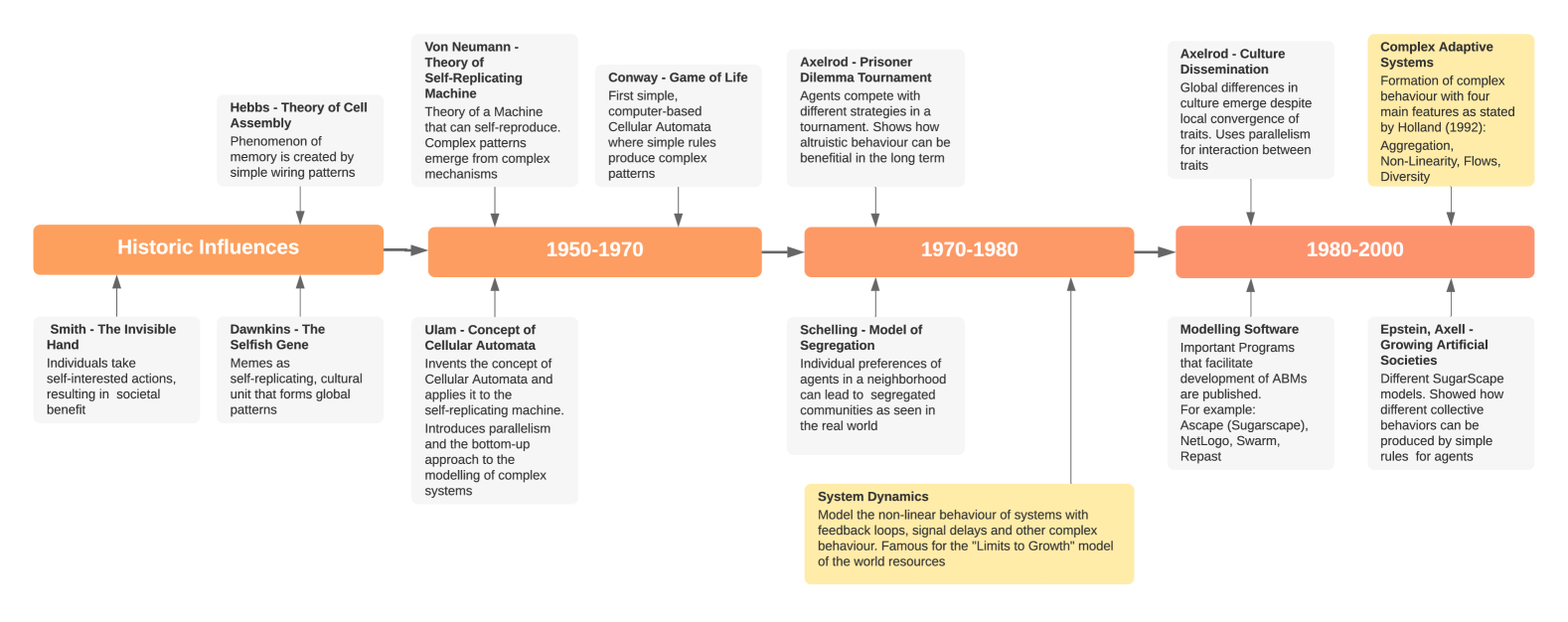
?figurename? 2.1: Timeline part one of two of agent-based modeling from the social sciences perspective from Carl Orge Retzlaff et al. [2]. Figure taken from [2], split in two parts, and used under the MIT license.

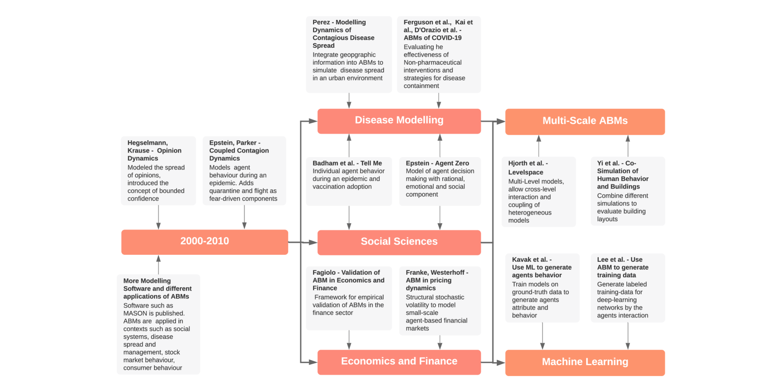
?figurename? 2.2: Timeline part two of two of agent-based modeling from the social sciences perspective from Carl Orge Retzlaff et al. [2]. Figure taken from [2] split in two parts and used under the MIT license.

2.2.2 Biological Cell and Tissue Models

ABM is extensively used in biology to model cancer [8, 10, 23, 11, 24, 25, 26, 27, 28, 29, 30, 31, 32, 33, 34, 35, 36, 37, 38], the nervous system [39, 40, 41, 42, 43, 13, 40, 44, 45, 46], morphogenesis [47, 48, 49, 50, 51, 52, 53, 54] biofilms [55, 56, 57, 58, 59, 60, 61], and many more [210, 211, 212, 213]. Simulations in these fields are often multi-scale to simulate processes that occur on different temporal or spatial scales, for example, cell division and diffusion. Development and validation of these models often include laboratory experiments that have an impact on each other [214]. The laboratory results are used to improve the model, which may necessitate further validation and, consequently, additional laboratory experiments if the data is unavailable.

An important subgroup is models to study cancer development [8, 10, 23, 11, 24, 25, 26, 27, 28, 29, 30, 31, 32, 33, 34, 35, 36, 37, 38] which investigate the pathogenesis, invasion, interaction with the vascular system, and responses to treatment. One advantage of the agent-based approach is its ability to integrate multiple data sources such as imaging or gene expression [26] and consider various interactions. Agents are typical cells, subcellular structures, or larger tissue components like a vessel segment. Cells may incorporate a state machine to distinguish between hypoxic, proliferative, quiescent, or necrotic conditions [10]. Spatial environments are typically used in agent-based cancer models, and the mechanical properties of the tissue are modeled using pairwise forces between agents. Metzgar categorizes the implementation of these models as on-lattice and off-lattice [27]. On-lattice methods include the already mentioned cellular automaton and the cellular Potts model (CPM) [215] extension, in which agents can occupy multiple grid positions. Off-lattice methods eliminate the constraints of discrete grid elements, allowing the agent to occupy any position in space.

In neuroscience, researchers use ABM to model the growth of neurons [39, 40, 41, 42, 43], the lamination of the cerebral cortex [13, 40], or neurodegenerative diseases [44]. Neurons can be modeled as a tree of neurite segment agents, which elongate, retract, branch, bifurcate, form synapses, and grow toward attracting chemical cues [39].

2.2.3 Epidemiology

Agent-based modeling allows for more realistic simulations of epidemiological questions and provides insights into the causal mechanisms [87, 88, 89, 90, 91, 92, 93, 94, 95, 96, 97, 98, 99, 100, 101, 102, 103, 104, 105, 106, 107, 108, 109, 110, 111, 112, 113, 114, 115, 116, 117], which provides benefits over compartmental models [216, 217]. Epidemiological applications include modeling the dynamics of infectious disease spread (such as COVID-19 [87, 88, 89, 90, 91, 92, 93, 94, 95, 96, 97, 98, 99], influenza [100, 101, 102, 103], malaria [218, 219, 220, 221, 222], and HIV [104, 105, 106]), assessing public health interventions [89, 90, 91, 92, 198, 93, 94, 96, 99, 223], epidemic forecasting [109, 97, 108], appraising pandemic preparedness and response [98, 107, 224], understanding the dynamics in urban areas [110, 111], and more [114, 115, 116, 117].

ABM allows epidemiological models to generate heterogeneous populations of agents (i.e., people) that may consider personal risk factors, the settlement structure of a region, movement patterns, and personal preferences (e.g., vaccination hesitancy [112, 113]). Recent work, for example, incorporates data from the Dutch National Statistics Bureau to more accurately model the spread of COVID-19 and their corresponding hospitalizations [87]. Another model from Ozik et al. provides actionable results and guided decision-making during the COVID-19 pandemic [88]. This work also reported the detection of health inequalities in the population, which can be a valuable insight to improve the future healthcare system.

2.2.4 Medicine

The application of agent-based modeling in medicine is multifaceted. Besides use cases that overlap with biology (Section 2.2.2) and epidemiology (Section 2.2.3), ABM is used for treatment planning [23, 11, 24, 25], chronic disease management [72, 73, 74, 75, 76, 77, 78, 79, 80, 81, 82, 83, 84], healthcare system optimizations [225, 84, 226, 227], immune system response [62, 63, 64, 65, 66, 67, 68, 69, 70, 71], pharmacodynamics [85], and others.

ABM’s strength lies in its ability to personalize treatment planning by enabling mechanistic models that consider a patient’s individual attributes. This personalized medicine approach may improve decision-making over phenomenological models that depend on clinical experience and possibly limited patient data. Cogno et al., for example, laid the groundwork for one such mechanistic model in their simulation of radiation-induced lung injury [23, 11, 24, 25] using BioDynaMo (Figure C.3).

Chronic diseases, including diabetes, obesity, cardiovascular diseases, and multimorbidities, negatively affect the patient’s life and the healthcare system as a whole [72]. For patients, these diseases often lead to long-term physical discomfort, reduced quality of life, and reduced life expectancy. Healthcare systems are under substantial financial strain due to the high prevalence of these diseases. Agent-based models are used to study and improve the management and prevention of chronic diseases [72, 73, 74, 75, 76, 77, 78, 79, 80, 81, 82, 83, 84] to improve the patient’s well-being and the cost-effectiveness of medical interventions.

Agent-based models are also used to optimize the processes in a healthcare system, such as a hospital emergency department. These models help to study policies to reduce patients’ waiting and admission time, cost of care, and undesirable treatment outcomes [225, 84, 226, 227].

2.2.5 Social Sciences

The ABM paradigm aligns well with the study of human interactions and the dynamics of a society [2]. Researchers studied cooperation [19], income inequality [195], reasoning [118], culture dissemination [119], and opinion dynamics [120]. For example, Axelrod studied the question “Under what conditions will cooperation emerge in a world of egoists without central authority?” [228]. Together with Hamilton, they invited experts to submit a program to compete in a tournament on the prisoner’s dilemma [229]. The prisoner’s dilemma is a game theoretical problem with two players, each of whom can choose between two different actions: cooperation or defection. Table 2.1 shows the rewards for the four possible states. Defection would lead to the highest expected reward without knowing the other player’s choice. For cooperation to emerge, the prisoner’s dilemma has to be played repeatedly.

This research maps naturally to agent-based modeling for four main reasons. First, the different strategies are translated into agent behaviors, which can involve complex, non-linear actions. Second, the focus lies on the emergence (of cooperation), which is a key feature of ABM (Section 2.1.3). Third, Axelrod was also interested in evolutionary dynamics, which is another key strength of ABM. Fourth, the agent-based model can help to understand the conditions that lead to cooperation or the robustness of these conditions.

In Axelrod’s tournament, each strategy was evaluated against every other one. The strategy with the highest reward turned out to be the simplest one: the strategy began with cooperation and then mirrored the opponent’s previous choice in the current round (i.e., tit-for-tat) [19]. Axelrod writes that this strategy could also be observed in trench warfare during World War 1: “[u]nits actually violated orders from their own high commands in order to achieve tacit cooperation with each other [i.e., the antagonist]” [228].

Player 1 / Player 2	Cooperate	Defect
Cooperate	(3, 3)	(0, 5)
Defect	(5, 0)	(1, 1)

?tablename? 2.1: Reward matrix for the prisoner’s dilemma based on [19]. Tuples represent the reward for (Player 1, Player 2).

2.2.6 Finance and Economics

Robert Axtell and Doyle Farmer provide a thorough overview of the applications of ABM in finance and economics [122]. Research topics include market models, micro- and macroeconomics, stock markets, banking regulations, systemic risk modeling, housing markets, and more [122]. Studying the origin of price changes, agent-based financial market models were able to qualitatively and quantitatively reproduce the following statistical properties of financial markets: “autocorrelation of price returns, autocorrelation of volatility, and the marginal distribution of price changes” [122].

2.2.7 Other Fields

The use of ABM is not restricted to the mentioned areas only; it is applied across various fields, ranging from agriculture [146, 230, 231, 232, 233, 234, 235, 236, 237] to zoology [147], and numerous other fields [146, 147, 148, 149, 150, 64, 151, 152, 153, 154, 155, 156, 157, 158, 159, 160, 161, 162, 163, 164, 165, 166, 136, 137, 138, 139, 140, 141, 142, 143, 144, 145, 124, 125, 126, 127, 128, 129, 130, 131, 132, 133, 134, 135].

2.3 Why Agent-Based Modeling?

The ABM paradigm was developed in response to the growing need for more flexibility and realism, driven by advancements in computing power. Researchers sought to liberate themselves from artificial constraints and assumptions necessary to keep the model mathematically tractable, which includes “linearity, homogeneity, normality, and stationarity" [190, 238]. These assumptions are not limited to mathematical aspects but can also be based on domain-specific factors. Axtell and Farmer provide two examples from economic models: perfect arbitrage and rational behavior [122]. Arbitrage allows investors to exploit price differences on different market places to make a profit. Perfect arbitrage describes a situation in which the trades of the investor are risk-free [239]. In economics, rational behavior describes the actions of an individual (i.e., homo oeconomicus), who acts in self-interest and makes consistent choices [240]. These two idealized assumptions are incorporated into economic models. ABM allows economists to deviate from these assumptions and create models that are more realistic [241].

Agent-based models offer the ability to incorporate heterogeneity, local variations, nonlinearity, and the assimilation of various data sources [87]. Unlike AI-based models, agent-based models, which are rooted in fundamental principles, produce simulation results that are easier to explain [26, 242]. Agent-based modeling is particularly suitable when the developmental aspect is a crucial component of the model because the simulation 1) evolves over time, 2) allows for heterogeneous agents and behaviors, 3) supports feedback loops through agent and environment interactions, and 4) excels in capturing emergent behavior. Examples include cancer growth studies [8, 10, 23, 11, 24, 25, 26, 27, 28, 29, 30, 31, 32, 33, 34, 35, 36, 37, 38] and development of the cerebral cortex [39, 40, 41, 42, 43, 13, 40, 44, 45, 46].

2.3.1 A Comparison to Other Modeling Paradigms

2.3.1.1 Equation-Based Modeling

In equation-based modeling (EBM) [243], a system’s observables are described with a set of (differential) equations. EBM is well-suited to describe physical systems like heat transfer, electromagnetism, or fluid dynamics. However, solving or analyzing specific characteristics using the equations may necessitate properties like differentiability or smoothness.

To illustrate the difference between ABM and equation-based modeling [243], we compare a simple epidemiological model that divides the population into three groups: susceptible, infected, and recovered (SIR) [216]. This model can be defined with three differential equations that depict the change over time: $dS/dt=-\beta SI/N$, $dI/dt=\beta SI/N-\gamma I$, and $dR/dt=\gamma I$. $S$, $I$, and $R$ are the number of susceptible, infected, and recovered individuals, $N$ is the total number of individuals, $\beta$ is the mean transmission rate, and $\gamma$ is the recovery rate.

These equations can be solved analytically [244] or numerically. An agent-based implementation with behaviors for movement, infection, and recovery is shown in Section 4.6.3. From these three behaviors, the same observables emerge through agent interactions. While the equation-based model is computationally (significantly) more affordable than an agent-based model, it is also quite rigid. Although variations with different compartments exist for incorporating properties of various infectious diseases, the agent-based model can be extended in almost limitless ways. The following list provides three examples to enhance realism of an epidemiological model using ABM.

• Movement patterns could encompass activities such as going to work, school, shopping, and socializing with friends and family.

• The initial agent population could be generated to reflect the country’s settlement structure.

• Risk factors that influence disease progression and hospitalization could be added to the agents.

These enhancements may enable scientists to examine various intervention methods and determine when hospitals become overwhelmed. For detailed agent-based epidemiological models, readers are referred to [87, 88].

2.3.1.2 System Dynamics

System Dynamics (SD) is another top-down approach to describe the dynamics of a complex system [245], initially developed for inventory control [246]. The model is often represented as a flow chart that contains the following key elements: stocks (i.e., the observables), flows between the stocks, and feedback loops. Figure 2.3 shows the previously described SIR model (Section 2.3.1.1) implemented in SD [3], which contains three stocks (susceptible, infected, and recovered), two flows (infection rate, and recovery rate), and three feedback loops (contagion, depletion, and recovery).

SD is well-suited for examining the high-level dynamics of a complex system that does not require any heterogeneity among its components. One of the best-known SD models is “The Limits to Growth” from Meadows et al. [247], which studies population and resource dynamics.

Despite the significant difference between SD and ABM (top-down versus bottom-up, deterministic versus stochastic), Macal showed that the set of SD models is a subset of ABM models, which he calls the “Agency Theorem” [248]. Thus all well-formed SD models can be translated into an equivalent agent-based model [248].

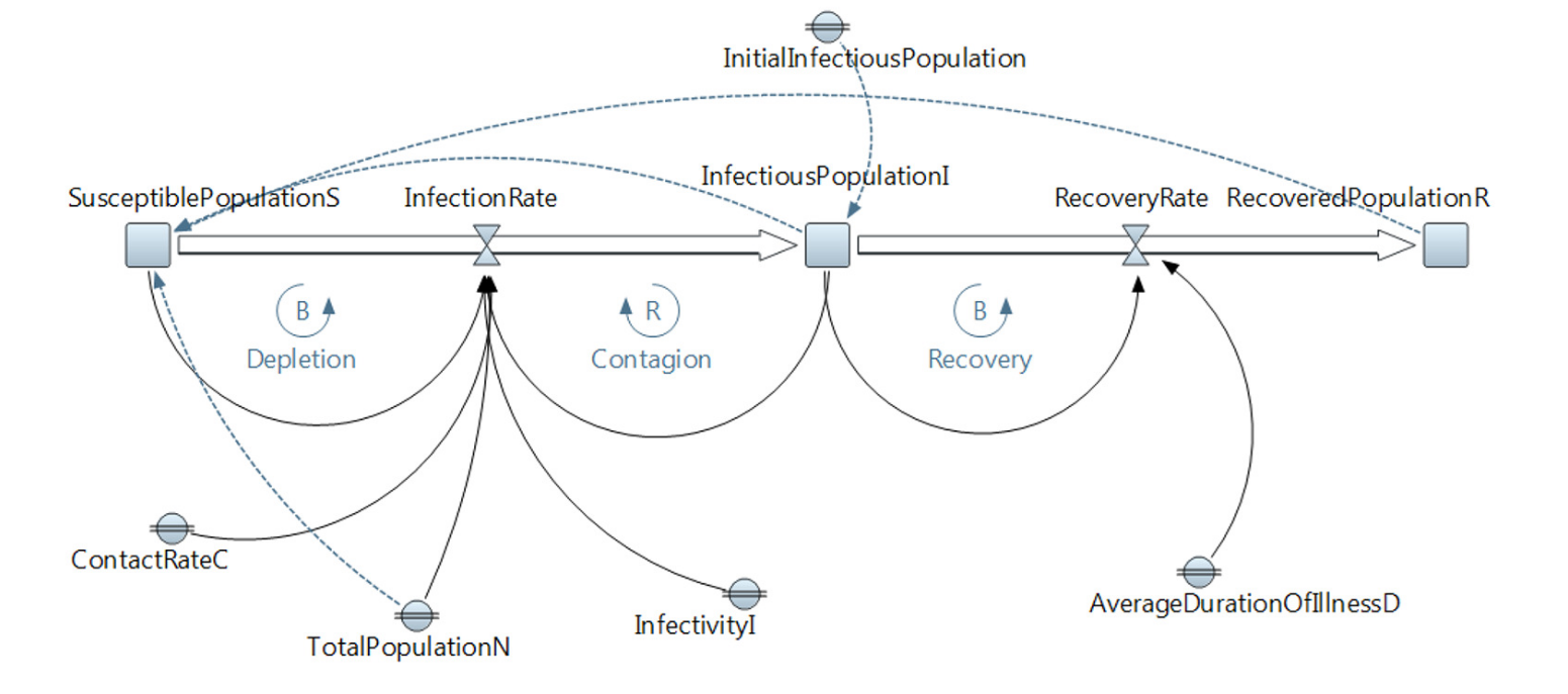
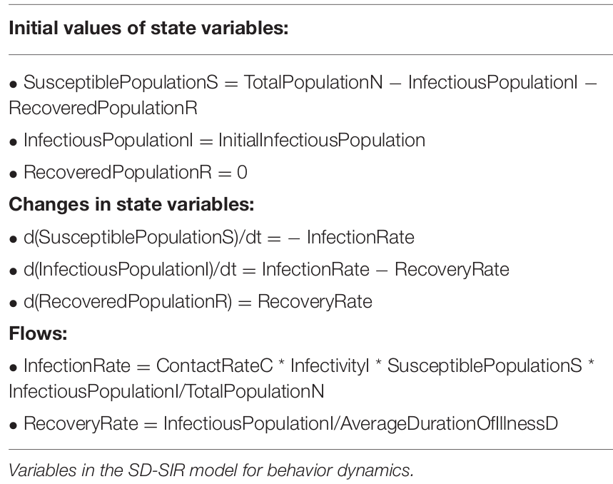
?figurename? 2.3: Implementation of the SIR model using system dynamics from Pietro Cipresso et al. [3]. Figure taken from [3] without modification and used under CC BY 4.0.

2.3.1.3 Discrete-Event Simulation

Discrete-event simulation (DES) [249, 250, 251] is a modeling method in which the simulation is assessed at specific time points triggered by an event. Events may be random variables that are sampled from a probability distribution. The event-driven nature of DES is in contrast to ABM where time evolves the simulation state [252]. DES is commonly used in operations research to model and optimize queuing systems [253]. DES is, for example, used in hospitals [254] to answer questions about mean waiting time, probability of waiting (longer than X minutes), or resource utilization [251]. These metrics are determined by aggregating the results of multiple simulation runs.

DES and ABM differ in several ways: top-down versus bottom-up approach, centralized versus decentralized control, passive versus active entities, and the presence of queues versus their absence [255].

2.3.1.4 Monte Carlo Simulation

The Monte Carlo method is a generic way of using random numbers as input to a problem for simulation, estimation, or optimization [256]. This method can, for example, be used to estimate the value of $\pi$ [257]. This estimation uses the fact that the area of the circle segment divided by the square is $\frac{\pi}{4}$. Thus, by estimating the two areas, one can estimate $\pi$ (Figure 2.4). The Monte Carlo method achieves this by: 1) defining points in 2D space as the input, 2) sampling points from a uniform distribution, 3) placing them on the square, and 4) aggregating the results: counting the points within distance of 1 from the origin as well as the total number of points. The estimation for $\pi$ is then $\frac{4\times r}{r+b}$, where $r$ and $b$ correspond to the number of red and blue points in Figure 2.4. This simple yet powerful method is widely used in physics, chemistry, mathematics, statistics, economics, and finance [256].

!

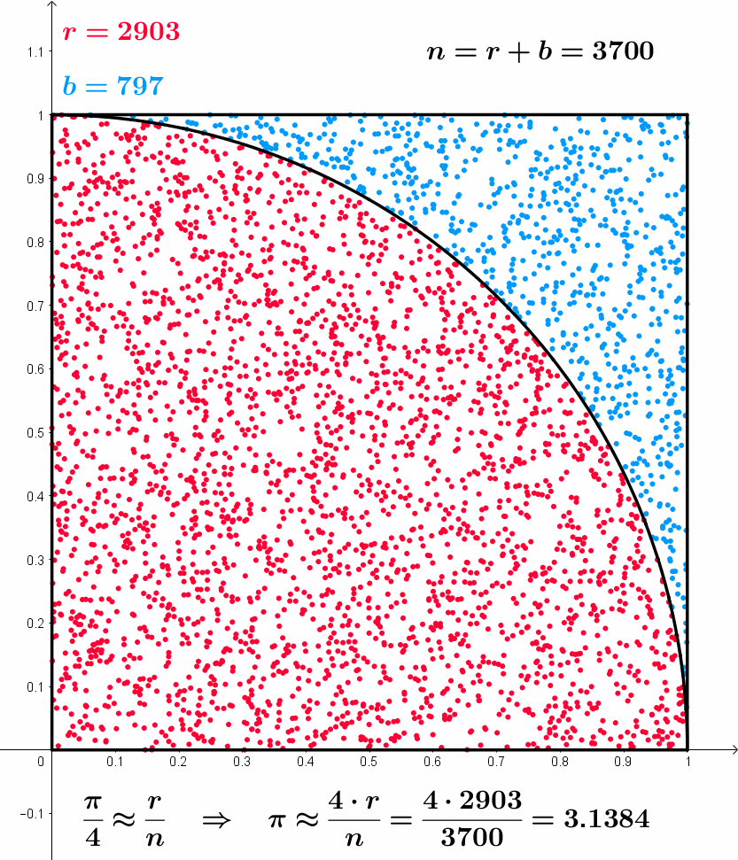
?figurename? 2.4: Estimation of $\pi$ using the Monte Carlo method. Figure taken from [4] and used under CC BY 4.0. One frame was extracted from the animation.

Based on the example of calculating $\pi$ mentioned earlier, it’s evident that MCM and ABM are fundamentally different. While MCM is centered on random sampling for estimating quantities, quantifying uncertainties, or optimizing functions [256], it cannot simulate interactions between individual entities and emergent behavior like ABM can.

2.3.1.5 Data-Driven Modeling

Traditional simulation methods, as described in Section 2.3.1.1–2.4 for example, can be classified as mechanistic models. Mechanistic models are built on causal relationships by combining fundamental physical, chemical, biological, or domain-specific principles [242, 258, 259, 260, 261, 262, 263]. Consequently, mechanistic models lead to interpretable results and can be used to make predictions once validated. However, mechanistic models are often computationally expensive, require deep domain knowledge to build, and pose challenges in integrating multiple sources of large unstructured data [242].

Data-driven modeling (DDM) [264, 265, 266, 267, 268, 269, 242] addresses these challenges by using machine learning and artificial intelligence techniques to train models that can make predictions about complex systems based on the patterns extracted from the data. Training typically necessitates access to large datasets. Data-driven models extract statistical correlations from these datasets rather than the causal relationships used in mechanistic models [242]. Once the model is trained, inference (i.e., “simulation” ) can be orders of magnitude faster than a simulation with a mechanistic model [270, 271]. This execution speed improvement is utilized for constructing surrogate models, i.e., models that serve as substitutes for costly mechanistic models in parameter optimization and sensitivity analysis [272, 273, 274, 275, 276, 277, 278, 279, 280, 281, 282, 283, 284, 285, 286].

However, DDM are not only used to approximate mechanistic models, but can also significantly outperform their capabilities. This potential has been impressively demonstrated by AlphaFold [287, 288, 289, 290], a machine-learning approach to predict the 3D shape of proteins based on their amino acid sequence, which is a long-standing problem in biology. AlphaFold won the CASP13 [291] and CASP14 [292] protein folding prediction challenge with a large margin, which is considered a scientific breakthrough [293].

Baker et al. [242] point out that the strengths and weaknesses of mechanistic and data-driven modeling are inverted and advocate for a combination of the two approaches [294]. This combination can be achieved in at least two ways. First, by using physics-informed machine learning techniques that incorporate mechanistic elements into the training process to achieve better results [295, 296, 297, 298, 299, 300, 301, 302, 303]. Second, by utilizing data-driven methods to extract relevant patterns from a data set, which are then used as part of a mechanistic model [242].

2.3.1.6 Hybrid Approach

The transition between the presented modeling approaches is often fluid [196]. Many models often employ a hybrid approach to harness the advantages of various modeling paradigms. Tissue models in biology often contain scalar or vector fields described as ordinary/partial differential equations, for example, to simulate substance diffusion [10] or heat transfer [183, 184]. To simulate radiation-induced lung tissue damage, Nicolo Cogno et al. integrate an agent-based model with Monte Carlo simulation and equation-based substance diffusion [23, 11]. In this model, the agent-based model is used to simulate the tissue, while the Monte Carlo simulation provides the radioactive dose for each cell. There are also works that combine ABM with SD [304] and DES [305].

2.4 How are Agent-Based Models Developed?

Agent-based models are developed iteratively [214, 9]. This approach allows starting with a simple, easier-to-understand model and gradually adding complexity as needed. In the beginning, modelers have to be clear about their modeling goal. Do they want to predict a certain observable of a complex system, or are they more interested in explaining a specific mechanism [21]?

From this goal, the agent-based model definition can be derived by making simplifying assumptions of the complex system under investigation [306] in a step by step manner. There are five steps.

Step 1: Entity Definition.

The modeler must define the main entities of the agent-based model: agents, behaviors, and the environment. The definition of an agent includes its attributes and functionality. To return to the epidemiological SIR model presented earlier (Section 2.3.1.1), agents can be defined as simple persons with a position in three-dimensional space and an attribute that determines the person’s state (susceptible, infected, or recovered). This agent type’s functionality includes changing the position and transitioning between the three SIR states. Afterward, the modeler must define the behaviors of these agents and how they interact. A simple model could define the following behaviors for movement, infection, and recovery: 1) move randomly, 2) become infected with probability $p_{i}$, if there is an infected agent within distance $d$, and 3) recover with probability $p_{r}$. This model would use a spatial environment, which supports agents’ interaction if they are within distance $d$. This model is explained in more depth in Section 4.6.3.

Once the modeler has defined the main components, the simulation’s initial state must determined, by answering questions like: How are the agents initially distributed in space? How many infected agents are there in the beginning and how are the distributed?

Step 2: Model Implementation.

The so far pen-and-paper model is cast into code in the implementation stage. To do that quickly and effectively, a modular simulation engine is needed that supports extension and modification without altering its internals. Ideally, the simulation platform already contains the necessary functionality and model building blocks, such that the modeler only has to select and connect the required pieces. Developing automated unit and integration tests is another important aspect. Testing helps to achieve a high-quality implementation, and helps to save development time. Finding a software error in a stochastic multi-million agent simulation is considerably more time-consuming than ensuring correctness by writing automated tests.

Step 3: Parameter Calibration.

After the simulation is implemented, the modeler has to determine the values for all parameters that have been added to the model as placeholders. Some parameters can be extracted from the literature , while others have to be determined using calibration and optimization. In the SIR model, for example, the recovery probability for a specific disease may be extracted from the literature [307], while the infection radius has to be determined through parameter calibration. To do that, the simulation is repeatedly executed with different parameter values, with the goal of minimizing an objective function. In the SIR model, the objective function may be defined as the mean squared error of the simulation result compared to the EBM model result. An optimization algorithm (e.g., particle swarm optimization [308]) determines the parameters for the next simulation execution based on the previous simulation results.

Step 4: Model Validation.

The model is validated with data separately and independently from the parameter calibration stage. This stage verifies that the model and its parameters accurately reflect the complex system under consideration. The validation can be quantitative or qualitative, depending on the use case and may include sensitivity analyses to investigate the uncertainty of the simulation results based on the input parameters.

Step 5: Model Usage.

The model is used for its intended purpose either to “predict, explain, guide data collection, discover new questions” [21] and more. Additional validation may be needed to validate predictions beyond the observables (e.g., the number of susceptible, infected, and recovered agents) used in the previous steps.

If the simulation results in steps two to five are not satisfactory, the modeler returns to the first step and reevaluates the assumptions and simplifications based on the insights of the current development iteration.

2.5 Challenges of Agent-Based Modeling

Although ABM has been successfully used to model complex systems in many domains, this modeling paradigm also faces several challenges, which we cover in this section.

Performance and Scalability.

For many agent-based models, the computational cost of simulating a vast number (e.g., millions or billions) of individual entities, exacerbated by the need to execute a simulation many times, is a key limitation [87, 10, 41, 13, 309]. Therefore, modelers are restricted by the number of agents they can simulate or by the complexity of the agent behaviors.

Parameter Calibration.

The number of model parameters in ABM can become large quickly as more details are incorporated into the model. Modelers face the challenge to determine realistic values for each parameter, either from the literature or through parameter calibration. Besides the vast parameter space, calibration is made even more difficult by the non-determinism of many models, their non-linear nature, and limited amount of available data. Even with available data, the simulation engine’s performance constrains the number of model executions during parameter calibration, potentially resulting in suboptimal simulation outcomes [116].

Validation.

Validation is an important step to ensure that the model is in agreement with the real-world system before it can be trusted and used. Beharathy and Silverman write that ABM modeling “ha[s] often been criticized for relying extensively on informal, subjective and qualitative validation procedures” [310]. Several validation techniques exist, but unavailable data, the challenge of describing an agent-based model formally [311], or the absence of a standard approach makes the process difficult [117]. Validation techniques include 1) face validation that relies on domain experts to determine if the model results matches the real-world system qualitatively [310], 2) cross-validation which compares the results with the output of other models [310], 3) extreme value analysis to investigate the consistency or limitations of the model [310] and 4) comparison with a mathematical model [311].

No Standard Approach.

ABM’s versatility can also be seen as challenging, as there is often no standard approach to a modeling task, apart from the high-level development steps presented in the previous section.

Therefore, finding the right model complexity is difficult [117, 312] and makes the development time-consuming. Sensitivity analyses and approximate Bayesian computation might help to detect inputs that have little impact on the observables of the system and, therefore, indicate potential for model simplification [117].

In addition, emergent behavior, which is often the desired outcome of modeling, is a broad concept and thus difficult to manage. Predicting emergent behavior is challenging, if at all possible, and there is no universal test to ascertain its occurrence in a simulation [313, 190].

Proper Simulation Platforms.

Modelers rely on a simulation platform to handle the complex computational tasks. Ideally, these platforms should be high-performing, user-friendly, easy to learn, modular, flexible, well-documented, freely available, robust, cross-platform compatible, interoperable, high-quality, and provide all necessary building blocks. However, in reality, the available simulation platforms prioritize different requirements, resulting in shortcomings in other areas that complicate the modeler’s work. Given the diversity of the ABM field, flexibility and modularity are essential platform properties that are often overlooked. This shortcoming, in turn, increases development time and hinders innovation in ABM.

Challenges Addressed.

In this dissertation, we address the platform and performance challenges. We create and implement a simulation platform that provides a comprehensive range of agent-based functionality, is flexible and modular for easy addition of new features, seamlessly integrates with third-party software, and focuses on high-quality. We address the performance issue by utilizing parallel and distributed computing, addressing the memory bottleneck of today’s computing systems, leveraging ABM-specific characteristics to avoid unnecessary work, and reducing data transfers between distributed processes.

?chaptername? 3 Related Work

In this chapter, we will outline how our contributions (Section 1.4) compare to the existing work in the field. We will examine the key features of BioDynaMo/TeraAgent in relation to other agent-based simulators (Section 3.1), differentiate between prior work on optimization and our shared-memory (Section 3.2) and distributed optimizations (Section 3.3), provide context for our performance evaluation (Section 3.4), and also include a comparison with simulation tools beyond the agent-based domain (Section 3.5).

3.1 Other Agent-Based Simulators

Several ABM platforms have been published demonstrating the importance of agent-based models in complex systems research [186, 314, 39, 315, 316, 317, 318, 319, 320, 42, 321, 322, 323, 324]. In this section, we compare BioDynaMo’s/TeraAgent’s most crucial system properties with prior work.

3.1.1 Extreme-Scale Model Support

To our knowledge, TeraAgent is the only simulation platform capable of simulating 501.51 billion agents. The largest reported agent populations in the literature is from Jon Parker [325], who simulated a specialized epidemiological model with up to 6 billion agents and Biocellion [7], a distributed tool in the tissue modeling domain, with 1.72 billion agents. Other distributed platforms exist [326, 327, 328, 329, 316], but have not shown simulations on this extreme scale.

The NeuroMaC neuroscientific simulation platform [42] claims to be scalable, but the authors do not present performance data and present simulations with only 100 neurons. Therefore, BioDynaMo’s ability to simulate large-scale neural development, which we demonstrate in Chapters 4 and 5, is, to our knowledge, unrivaled.

3.1.2 General-Purpose Application Area Support

Many ABM platforms focus on a specific application area, for example: bacterial colonies [314, 323, 319, 318], cell colonies [321, 320, 322], and neural development [39, 315, 42]. Pronounced specialization of an ABM platform may prevent its capacity to adapt to different use cases or simulation scenarios. In contrast, BioDynaMo can be adapted to many different fields due to its modularity and extensibility as we show in Chapter 4 (and as also shown by various other works [23, 24, 25, 11, 10, 41, 87, 8, 9, 183, 184, 18, 17]). For example, BioDynaMo has been used to study (radiation-induced) lung injury [23, 24, 25, 11], vascular tumor growth [10], gliomas [8], country-scale COVID-19 hospitalizations [87], growth of pyramidal cells [41], the formation of retinal mosaics [9], cancer cell treatment with helium plasma jet [17], cancer drug pharmacodynamics [18], freezing and thawing of tissue [183, 184], spread of HIV in Malawi [182], development of the cerebral cortex [13], and other works that are currently in progress.

3.1.3 Quality Assurance

Automated software testing is the foundation of a modern development workflow. Unfortunately, several simulation tools [39, 319, 318, 315, 42, 322] omit these tests. Mirams et al. [320] recognizes this shortcoming and describes a rigorous development workflow in their paper. TeraAgent has over 600 automated tests (see Section 4.3.6) that are continuously executed on all supported operating systems to ensure high code quality. The open-source code base [330, 331, 332], tutorials (see Appendix E), and documentation not only help users get started (quickly) with modeling tasks, but also enable validation by external examiners.

3.2 Shared-Memory Performance Optimizations

In order to achieve high-performance and efficiency, we improve the performance of the shared-memory parallelized simulation engine with a series of optimizations. This section compares our memory layout optimization, improved neighbor search algorithm, and utilization of domain-specific knowledge with prior work.

3.2.1 Memory Layout Optimization

Data movement between main memory and processor cores is a fundamental bottleneck in today’s computing systems [333]. Recent research in computer architecture explores new approaches to address this bottleneck, such as processing-in-memory, i.e., placing compute capability closer to the data [334, 335]. Agent-based simulation tools are also negatively impacted by the data movement bottleneck (Section 5.6.3). We address this problem in software with a better memory layout that leads to more efficient bandwidth utilization and data reuse in processor caches. Space-filling curves [336, 337, 338] can improve the memory layout by aligning objects that are close in 3D space. Therefore, these curves are frequently used to optimize geometric data structures [339, 340] and molecular dynamics simulations [341, 342, 343]. To our knowledge, none of the other agent-based simulation frameworks (e.g., [344, 7, 345, 327, 186, 39, 346, 347, 348, 349, 42, 350, 329, 328, 351, 352, 316, 353]) use space-filling curves to improve the cache hit rate and minimize the amount of remote DRAM accesses. We introduce this proven technique to agent-based modeling and present a mechanism to determine the Morton order of a non-cubic grid in linear time.

3.2.2 Neighbor Search

Agent-based simulation platforms use various neighbor search algorithms: Delaunay triangulation [39], octree [354], and grid-based approaches [186, 316, 7]. Grids are also commonly used on GPUs [355, 339, 356, 357, 358]. Depending on the dataset and specific search query ([fixed-]radius neighbor search or k-nearest neighbors), the literature recommends different algorithms [359, 339]. Our contribution is the efficient implementation and integration of the uniform grid into the simulation engine (Section 5.3.1) and the insights into the performance differences for the agent-based workload (Section 5.6.9).

3.2.3 Omitting Unnecessary Work

In Section 5.5 we present a mechanism to omit the collision force calculation for static agents safely. The neuroscience simulation tool NeuroMaC [42] goes one step further and exclusively supports models where only the growth front of a neuron can change. This is probably a good optimization for this line of research but is too restrictive for BioDynaMo’s goal of becoming a general-purpose platform. Related work can also be found in the traffic simulation domain, in which Andelfinger et al. [360] proposes a mechanism to skip iterations of independent agents and fast-forward them to the next interaction time.

3.3 Distributed Performance Optimizations

In the distributed simulation engine, in which agents are distributed among multiple processes, information exchange is a key bottleneck. We address that challenge by optimizing serialization (i.e., packing agents into a contiguous buffer that can be transmitted) and reducing the amount of data transferred with delta encoding. The following section discusses related work in these two areas.

3.3.1 Serialization

There is a wide range of serialization libraries. Chapter 6 compares the performance against ROOT IO [361], which according to Blomer [362] outperforms Protobuf [363], HDF5 [364], Parquet [365], and Avro [366]. MPI [367] also provides functionality to define derived data types, but targets use cases with regular patterns, for example, the last element of each row in a matrix. TeraAgent’s agents are allocated on the heap with irregular offsets between them and, therefore, cannot use MPI’s solution.

3.3.2 Delta Encoding

Delta encoding [368] is a widely used concept to minimize the amount of data that is stored or transferred, which we apply to aura updates of the agent-based workload (Section 6.2.3). Other applications include backups [369], file revision systems such as git [370], network protocols [371, 372], cache and memory compression [373, 374, 375, 376], and more [377, 378]. We did not find explicit mention of this concept in the literature to accelerate the distributed execution of agent-based simulations.

3.4 Performance Evaluation

To our knowledge, this dissertation presents the most comprehensive performance analysis to date of an agent-based simulation platform. Existing platforms report only limited performance results, including simulation execution times and occasionally scalability analyses [39, 327, 7, 326, 345, 344]. Performance data can also be found in model papers [379, 380] and in works that focus on hardware accelerators [381]. We improve upon these works by providing an in-depth analysis of each performance-relevant component. Efforts in the direction of a standard agent-based benchmark have been made by Moreno et al. [382] and Rousset et al. [383]. However, these synthetic benchmarks fall short of representing a realistic range of agent-based simulations by over-simplifying memory access patterns and assuming that agents always move randomly. Compared to these, our benchmark simulations cover a broader spectrum of performance relevant simulation metrics (see Table 5.1). Chapter 5 and 6 in this thesis provide detailed performance analyses of the shared-memory and distributed simulation engine and the different use cases presented in Chapter 4.

3.5 Comparisons With Simulators Outside the Agent-Based Modeling Field

Particle-based simulations, i.e., simulations made of discrete particles that interact with each other , such as molecular dynamics (MD) [384, 385, 386], astrophysics (AP) [387], or computational fluid dynamic (CFD) [388] simulations often face similar computational challenges to improve the performance of large-scale simulations. Some agent-based models, for example cell sorting (Section 4.7.1), may also be seen as a particle-based method. LAMMPS [385], for example, also uses a grid-based structure to determine neighbors. While LAMMPS stores neighbor lists for each atom, which according to Thompson et al. [385] “consumes the most memory of any data structure in LAMMPS” BioDynaMo does not need these lists and therefore saves memory. BioDynaMo improves over LAMMPS and VASP [386] by sorting agents using a space-filling curve (Section 5.4.2) and using a custom memory allocator (Section 5.4.3) to reduce the memory access latency. A NUMA-aware thread allocation mechanism, as the one used in BioDynaMo (Section 5.4.1), is not needed in LAMMPS or VASP because both tools support distributed parallelism with MPI. In this work, we identify several computational challenges in ABM, which we tackle by using methods inspired by MD, AP, and CFD. The main difference between ABM and other particle-based applications is that the computations can vary significantly from each other in terms of arithmetic intensity, the number of considered neighbors, data access patterns, and more, thus posing diverse computational challenges.

?chaptername? 4 The BioDynaMo Platform

4.1 Introduction

Agent-based simulation (ABS) is a powerful tool assisting life scientists in better understanding complex biological systems. In silico simulation is an inexpensive and efficient way to rapidly test hypotheses about the (patho)physiology of cellular populations, tissues, organs, or entire organisms [389, 390].

However, the effectiveness of such computer simulations for scientific research is often limited, in part because of two reasons. First, after the slowing down of Moore’s law [168] and Dennard scaling [169], hardware has become increasingly parallel and heterogeneous. Most ABS platforms do not take full advantage of these hardware enhancements. The resulting limited computational power forces life scientists to compromise either on the resolution of the model or on simulation size [199]. Second, existing ABS platforms have often been developed with a specific use case in mind. This makes it challenging to implement the desired model, even if it deviates only slightly from its original purpose.

To help researchers tackle these two major challenges, we propose a novel open-source platform for biology dynamics modeling, BioDynaMo. We alleviate both of these problems by emphasizing performance and modularity. BioDynaMo features a high-performance simulation engine that is fully parallelized to utilize multi-core CPUs and able to offload computation to hardware accelerators (e.g. a GPU). The software comprises a set of fundamental biological functions and a flexible design that adapts to specific user requirements. Currently, BioDynaMo implements the neurite model and mechanical forces presented in [39], but these components can easily be extended, modified, or replaced. Hence, BioDynaMo is well-suited for simulating a wide range of biological processes in tissue modeling and beyond.

BioDynaMo provides by design five system properties:

• Agent-based. The BioDynaMo project is established to support an agent-based modeling approach which allows one to simulate a wide range of developmental biological processes. A characteristic property of agent-based simulations is the absence of a central organizational unit that orchestrates the behavior of all agents. Quite to the contrary, each agent is an autonomous entity that individually determines its actions based on its current state, behavior, and the surrounding environment.

• General purpose. BioDynaMo is developed to become a general-purpose tool for agent-based simulation. To simulate models from various fields, BioDynaMo’s software design is extensible and modular.

• Large scale. Biological systems contain a large number of agents. The cerebral cortex, for example, comprises approximately 16 billion neurons [391]. Biologists should not be limited by the number of agents within a simulation. Consequently, BioDynaMo is designed to take full advantage of modern hardware and use memory efficiently to scale up simulations.

• Easily programmable. The success of an ABS platform depends, among other things, on how quickly a scientist, not necessarily an expert in computer science or high-performance programming, can translate an idea into a simulation. This characteristic can be broken down into four key requirements that BioDynaMo is designed to fullfil:

  First, BioDynaMo provides a wide range of common functionalities such as visualization, plotting, parameter parsing, backups, etc. Second, BioDynaMo provides simulation primitives that minimize the programming effort necessary to build a use case. Third, as outlined in item “General purpose", BioDynaMo has a modular and extensible design. Fourth, BioDynaMo provides a coherent API and hides implementation details that are irrelevant for a computational model (e.g., details such as parallelization strategy, synchronization, load balancing, or hardware optimizations).

• Quality assured. BioDynaMo establishes a rigorous, test-driven development process to foster correctness, maintainability of the codebase, and reproducibility of results.

The main contribution of this chapter is an open-source, high-performance, and modular simulation platform for agent-based simulations. We provide the following evidence to support this claim: (i) We detail the user-facing features of BioDynaMo that enable users to build a simulation based on predefined building blocks and to define a model tailored to their needs. (ii) We present three basic use cases in the field of neuroscience, oncology, and epidemiology to demonstrate BioDynaMo’s capabilities and modularity. (iii) We show that BioDynaMo can produce biologically-meaningful simulation results by validating these use cases against experimental data or an analytical solution. (iv) We present performance data on different systems and scale each use case to one billion agents to demonstrate BioDynaMo’s performance.

4.2 Design Overview

4.2.1 Simulation Concepts

BioDynaMo is implemented in the C++ programming language and supports simulations that follow an agent-based approach. Figure 4.1 gives an overview of BioDynaMo’s main concepts, Figure 4.2 presents the abstraction layers, while Figure 4.3 illustrates its object-oriented design.

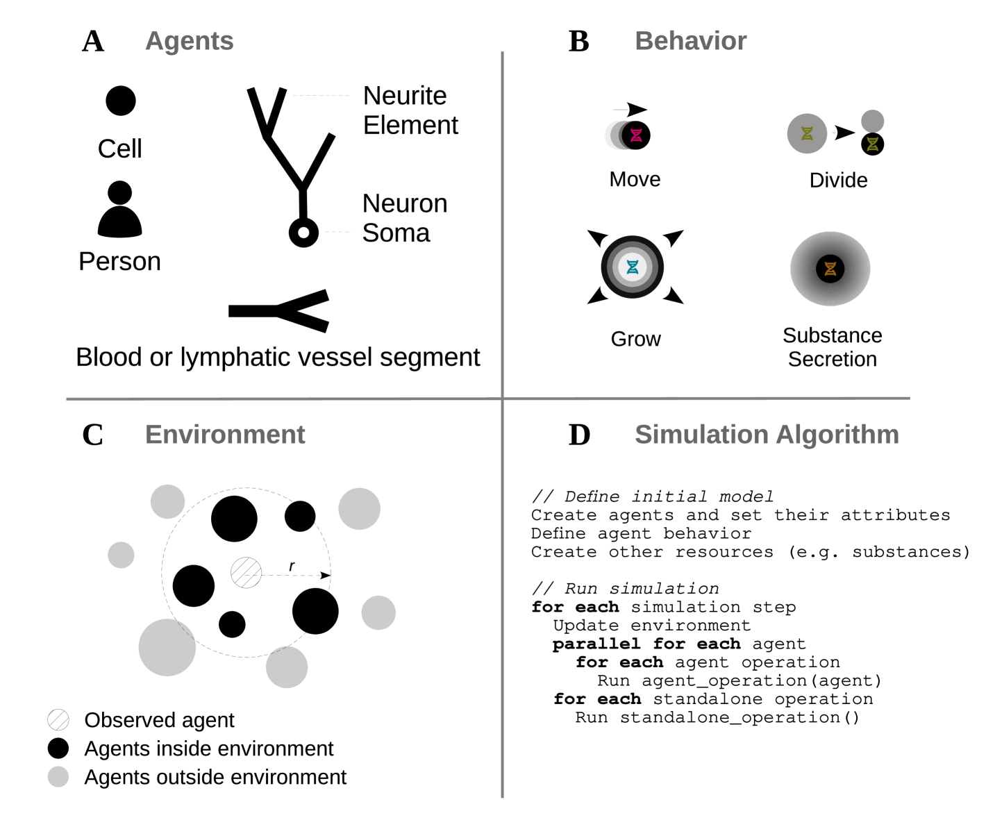
?figurename? 4.1: Simulation concepts. Agents (A) have their own geometry, behavior (B), and environment (C). (B) Agent behavior is defined in separate classes, which are inserted into agents. The update of an agent is based on its current state and its surrounding environment. (C) The environment is determined by radius $r$ and contains other agents or extracellular substances. The simulation algorithm (D) can be divided into two main parts: the definition of the initial model and the execution of the simulation.

An agent (Figure 4.1A) has a 3D geometry, behavior, and environment. There is a broad spectrum of entities that can be modeled as an agent. In the results section, we show examples where an agent represents a subcellular structure (neuroscience use case), a cell (oncology use case), or a person (epidemiology use case). Figure 4.1B shows example agent behaviors such as growth factor secretion, chemotaxis, or cell division. Behaviors can be activated or inhibited. BioDynaMo achieves this by attaching them to or removing them from the corresponding agent.

The Environment is the vicinity that the agent can interact with (Figure 4.1C). It comprises agents and other resources like chemical substances in the extracellular matrix. Surrounding agents are, for example, needed to calculate mechanical interactions among agent pairs.

Currently, the user defines a simulation programmatically in C++ (see Figure 4.1D and Section 4.6.4). C++ is a great choice in terms of execution speed, efficiency, and interoperability with high-performance computing libraries, but is harder to program in due to its lower level of abstraction (versus higher level languages like Java or Python). There are two main steps involved: initialization and execution. During initialization, the user places agents in space, sets their attributes, and defines their behavior. In the execution step, the simulation engine evaluates the defined model in the simulated physical environment by executing a series of operations. We distinguish between agent operations and standalone operations (Figure 4.1D). At a high level, an agent operation is a function that: (i) alters the state of an agent and potentially also its environment, (ii) creates a new agent, or (iii) removes an agent from the simulation. Examples for agent operations are: execute all behaviors and calculate mechanical forces. The simulation engine executes agent operations for each agent for each time step. Alternatively, standalone operations perform a specific task during one time step and are therefore only invoked once. Examples include the update of substance diffusion and the export of visualization data.

4.2.2 BioDynaMo Features

BioDynaMo is a simulation platform that can be used to develop agent-based simulations in various computational biology fields (e.g. neuroscience, oncology, epidemiology, etc.). Although agent-based models in these different fields may intrinsically vary, there is a set of functionalities and definitions that they have in common.

These commonalities can be divided into low- and high-level agent-based features and are an integral part of BioDynaMo. BioDynaMo also provides model building blocks to accelerate the development of agent-based models. The described layered architecture is shown in Figure 4.2.

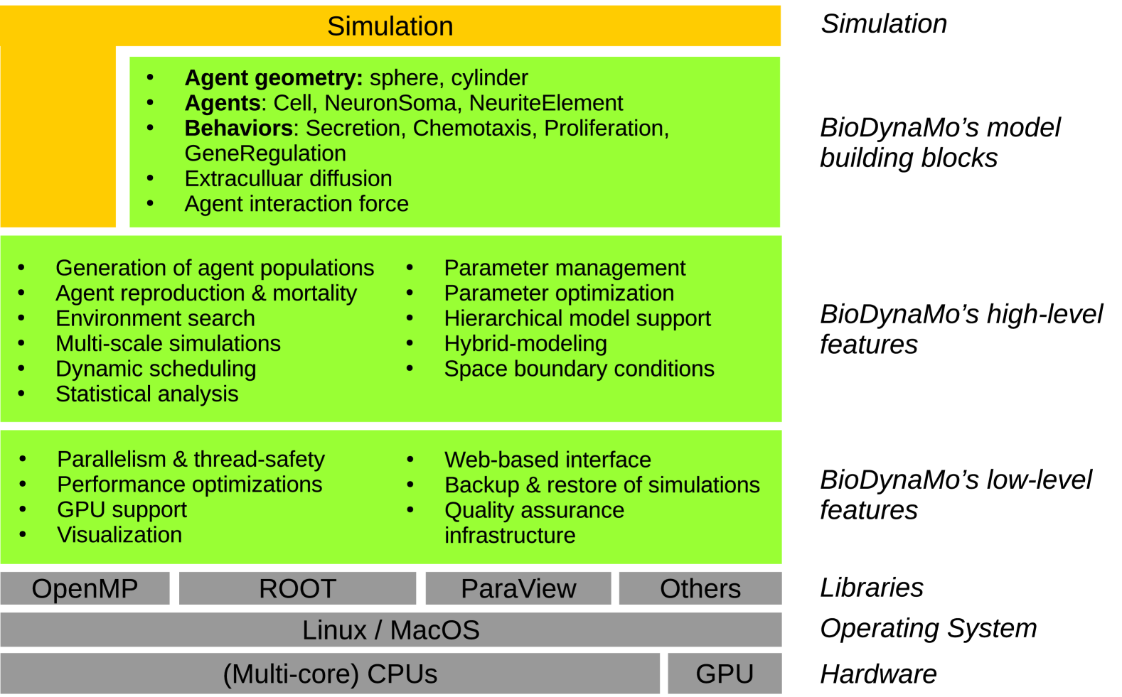
?figurename? 4.2: BioDynaMo’s layered architecture. BioDynaMo is predominantly executed on multi-core CPUs, is able to offload computations to the GPU, and supports Linux and MacOS operating systems. BioDynaMo provides a rich set of low- and high-level features commonly required in agent-based models. On top of these generic features, BioDynaMo offers model building blocks to simplify the development of a simulation. Even if BioDynaMo does not provide the required building blocks, users still benefit from all generic agent-based features (illustrated by the vertical extension of the “Simulation" layer).

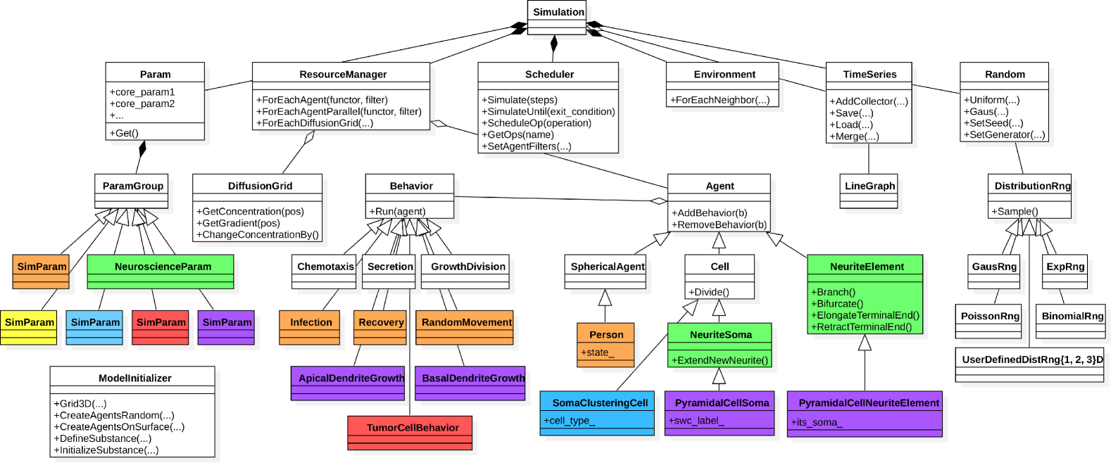
?figurename? 4.3: Software design and modularity. Overview of selected classes and functions that are important from the users’ perspective. Classes in white (BioDynaMo core) and green (BioDynaMo’s neuroscience module) are part of the current BioDynaMo installation. The remaining classes illustrate how we extended BioDynaMo to implement the use cases and benchmarks presented in this chapter (purple: neuroscience use case, red: oncology use case, orange: epidemiology use case, blue: soma clustering benchmark, yellow: cell proliferation benchmark). A complete list of BioDynaMo classes can be found at https://biodynamo.org/api.

4.3 Low-Level Features

The low-level features (Figure 4.2) form the foundation of BioDynaMo and provide crucial functionality responsible for high-performance execution and ease-of use. These features are mostly hidden from the user and require control only in exceptional situations.

4.3.1 Parallelism and Thread Safety

BioDynaMo exploits the inherent parallelism of agent-based models in which agents update themselves based on their current state, behavior, and local environment. BioDynaMo’s implementation uses OpenMP (https://www.openmp.org/) compiler directives to parallelize the loop over all agents (Figure 4.1D). In addition to parallelizing the execution of agent operations for each agent, standalone operations like updating the diffusion grid and visualization are parallelized separately (Figure 4.1D).

Synchronization between threads is only needed if agents modify their environment. In this case, two agents (handled by two different threads) might attempt to update the same resource in the local environment. This scenario occurs in the neuroscience use case in which neurite elements modify neighboring segments. Therefore, BioDynaMo provides built-in synchronization mechanisms to ensure that even if two threads try to modify the same agent or resource, data is not corrupted. There are two thread safety mechanisms to protect agents from data corruption: automatic and user-defined (Figure 4.4). Automatic thread safety uses the environment to prevent two threads from processing agents with overlapping local environments (A,C). This mechanism can be enabled with a single parameter, but might be too restrictive for some use cases. User-defined thread safety on the other hand offers more fine-grained control over which agents must not be processed at the same time, but likely requires additional input from the user (B,D).

Other resources that are modified by agents (e.g., the DiffusionGrid to simulate extracellular diffusion) need their own protection mechanism. This feature is used in the soma clustering benchmark where cells secrete a substance into the extracellular matrix.

For typical BioDynaMo simulations users do not need to control parallel execution and thread synchronization. This holds particularly true for all use cases and benchmarks presented in this chapter. Only for more advanced uses, like adding a new environment algorithm or adding a shared resource that is not an agent, users have to consider parallel execution.

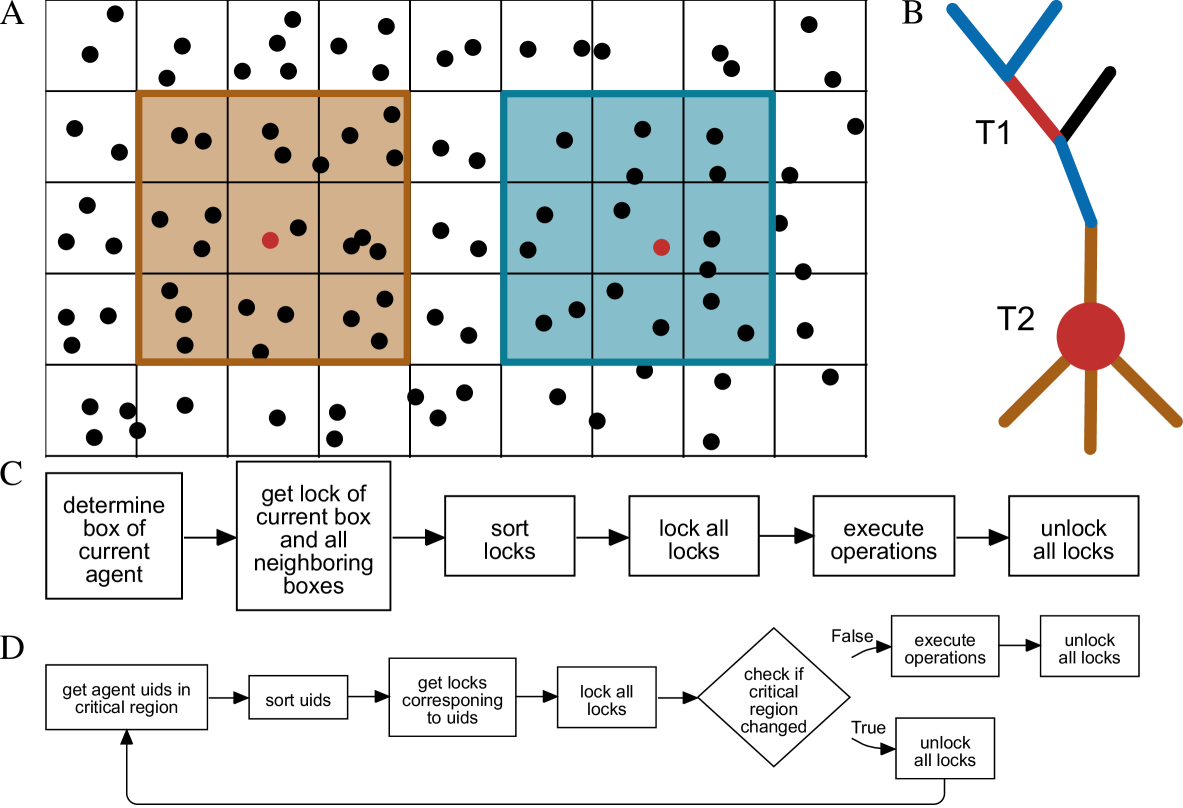
?figurename? 4.4: Thread safety in BioDynaMo. A: Currently updated agents in red and their local environment defined by the uniform grid in ocher and blue. B: Neuron model in which two different threads (T1 and T2) update the agents in red. Neighboring agents in ocher and blue might be modified during the update. C: Flow chart of the automatic thread safety mechanism, which ensures that the local environments in A do not overlap. D: Flow chart of the user-defined thread safety mechanism, which ensures that agents that might be modified (i.e., critical region) do not overlap.

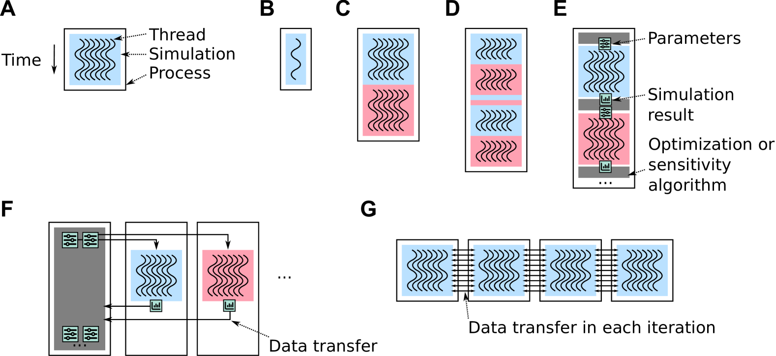
?figurename? 4.5: Parallelism modes. A: Multithreaded (default) execution. B: Serial execution. C–G can also be executed with one thread in each simulation block. C: Multiple simulations in the same process. D: Multiple simulations in the same process with alternating execution and potential exchange of information. E: Optimization or sensitivity analysis in the same process. F: Optimization or sensitivity analysis with multiple processes. G: Distributed execution (one simulation divided onto multiple servers).

Figure 4.5 provides an overview of BioDynaMo’s parallel execution modes. shows the default mode of the single-node simulation engine. All available CPU threads of the machine (i.e. laptop, workstation, or server) are utilized. The user can change the number of threads used. The thread number can be increased to oversubscribe the machine, or reduced down to one if the simulation is very small and the overheads outweigh the benefits of parallel execution . This mode is used for example in the performance evaluation in Chapter 5.6.6 to compare BioDynaMo with our serial baselines. – can also be executed with one thread per simulation block. shows that within the same process, multiple simulations can be executed. Simulations do not have to run until completion before the next simulation can be started. It is possible to switch between simulations and exchange information  . However, there can only be one active simulation at the same time within a process. In other words, within the same process, multiple simulations cannot be updated in parallel. This mode was used in [8]. uses the ability to execute multiple simulations in one process for optimization or sensitivity analysis with one process. This mode was used in the epidemiology use case to find the right simulation parameters for measles and seasonal influenza (Section 4.6.3). Hesam et al. [87] extends upon this solution by removing the restriction of one process. The authors develop an MPI-based solution in which the master rank is running the optimization or sensitivity algorithm. The algorithm generates new parameter sets, which are transferred to a free worker node. The worker executes the simulation using the parameters received and returns the result. Hesam et al. uses a modular design that allows for the easy replacement of the algorithm. This solution is part of the BioDynaMo installation. Duswald et al. [41] demonstrates that BioDynaMo integrates well with third-party software that externally provides the algorithm and worker management. Lastly, shows the distributed simulation engine which partitions one simulation and executes it using multiple processes. This important functionality is described in detail in Chapter 6.

4.3.2 Visualization

BioDynaMo currently uses ParaView [392] as a visualization engine. There are two visualization modes, which we refer to as live mode and export mode. With live mode, the simulation can be visualized during runtime, whereas with export mode, the visualization state is exported to file and can only be visualized post-simulation. Live mode is a convenient approach to debug a simulation visually while it is executed. However, this can slow down the simulation considerably if used continuously. In export mode, the visualization state can be loaded by the visualization package for post-simulation processing (slicing, clipping, rendering, animating, etc.). BioDynaMo can visualize substance concentrations and gradients (see Figure 4.21), and the geometry of the supported agents.

Furthermore, it is possible to export any agent’s data members. This information can then be used as input to ParaView filters, e.g., to highlight elements based on a specific property. The export of additional data members was used in Figure 4.21, for example, to color cells by their cell type.

4.3.3 BioDynaMo Notebooks

Jupyter notebooks [393] is a widely used web application to quickly prototype or demonstrate features of a software library. With notebooks, it is possible to easily create a website with inline code snippets that can be executed on-the-fly. ROOT expands these notebooks by offering a C++ backend in addition to the default Python backend. This allows us to provide a web interface to easily and quickly get started with BioDynaMo. Users do not need to install any software packages; a recent web browser is enough. It is also a convenient tool to interactively go through a demo or tutorial, which opens up possibilities to use BioDynaMo for educational purposes. BioDynaMo is the first agent-based simulation platform written in C++ that offers such an interface. BioDynaMo notebooks have already been successfully used to demonstrate and teach about pyramidal cell growth and were well-received by high-school students and teachers during CERN’s official teachers and students programs. Figure 4.6 shows an example of how a BioDynaMo notebook looks. This example gives a brief introduction to pyramidal cells and follows up with a step-by-step explanation of how to simulate their growth with BioDynaMo. Interactive visualizations in the browser give users quick feedback about the simulation status. Lastly, tutorials written as BioDynaMo notebooks can be executed as part of our continuous integration pipeline and ensure that documentation stays in sync with the codebase. In Supplementary Tutorial LABEL:ap:st01—LABEL:ap:st15 we use this feature to explain BioDynaMo to new users.

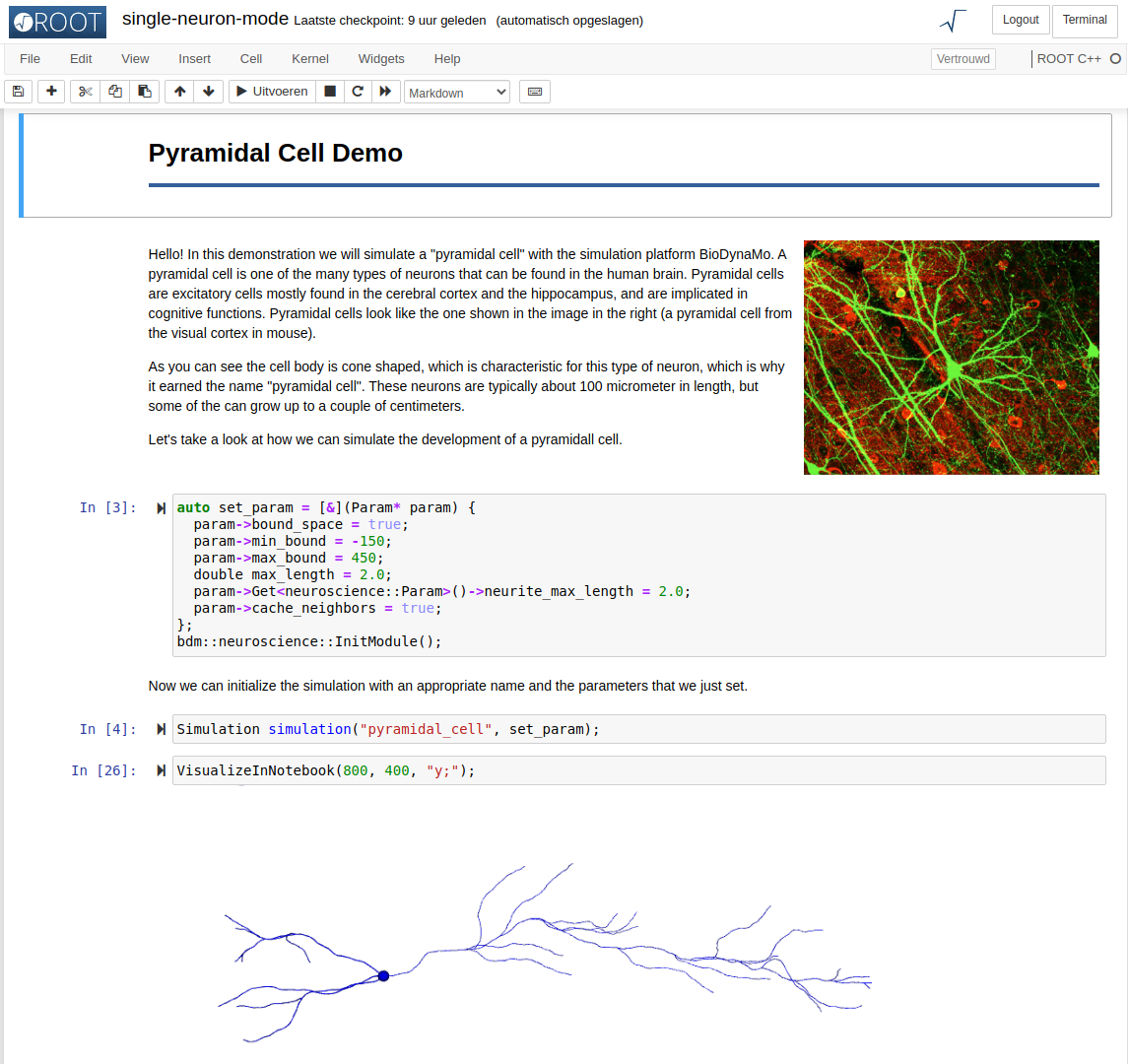
?figurename? 4.6: BioDynaMo notebook. A convenient web interface to create and run simulations in a step-by-step manner. The inlining of text and media makes it possible to provide extra information. A few intermediary blocks have been removed to fit the final simulation output on the screenshot.

4.3.4 Full Web-Based Development Environment

For advanced simulations that contain more code than manageable in a notebook or require the full BioDynaMo feature set, we provide a full web-based development environment, based on the Gitpod service [394]. To that extent, we package BioDynaMo in a docker image with Gitpod’s base image and customize Gitpod’s development environment. If the user clicks on a demo link on the BioDynaMo website, Gitpod creates a new instance based on this image. The user interacts with this instance via a browser-based VSCode [395] development environment. Figure 4.7 shows the welcome screen after clicking on the pyramidal cell growth demo link, which contains user instructions on how to proceed. The image below shows the opened code pane and the terminal with a successful execution of this demo simulation.

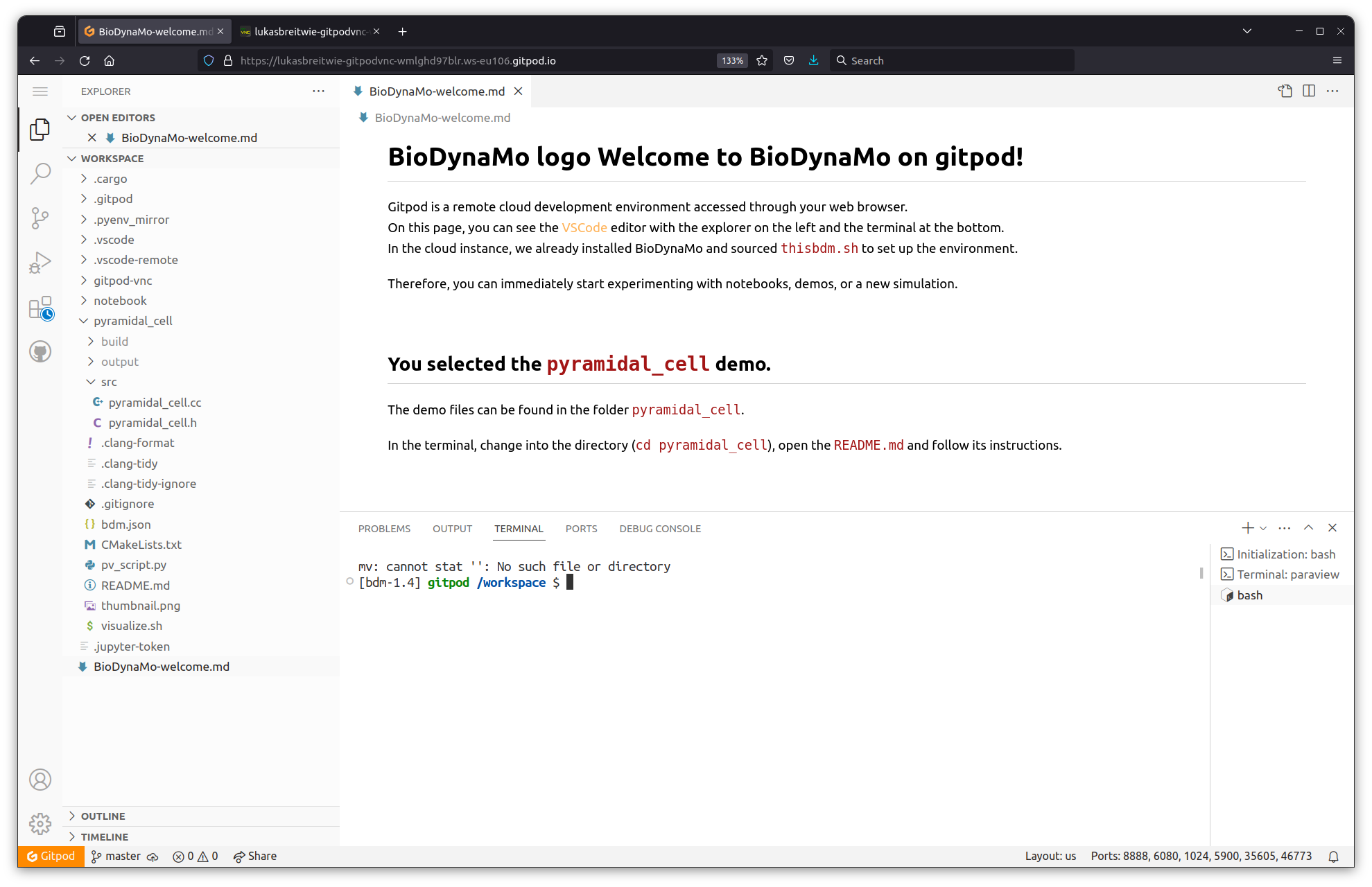
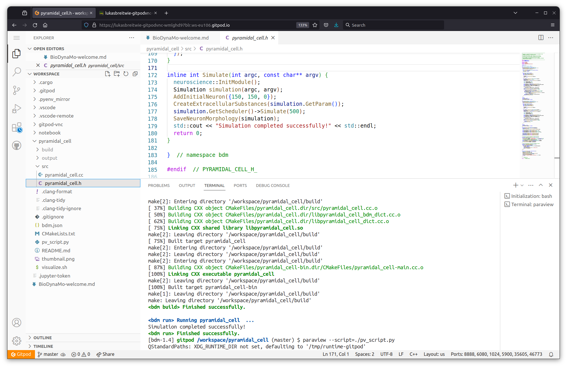
?figurename? 4.7: Web-browser-based development environment. Top: Welcome screen with user instructions. Bottom: Code pane and terminal with successful simulation execution.

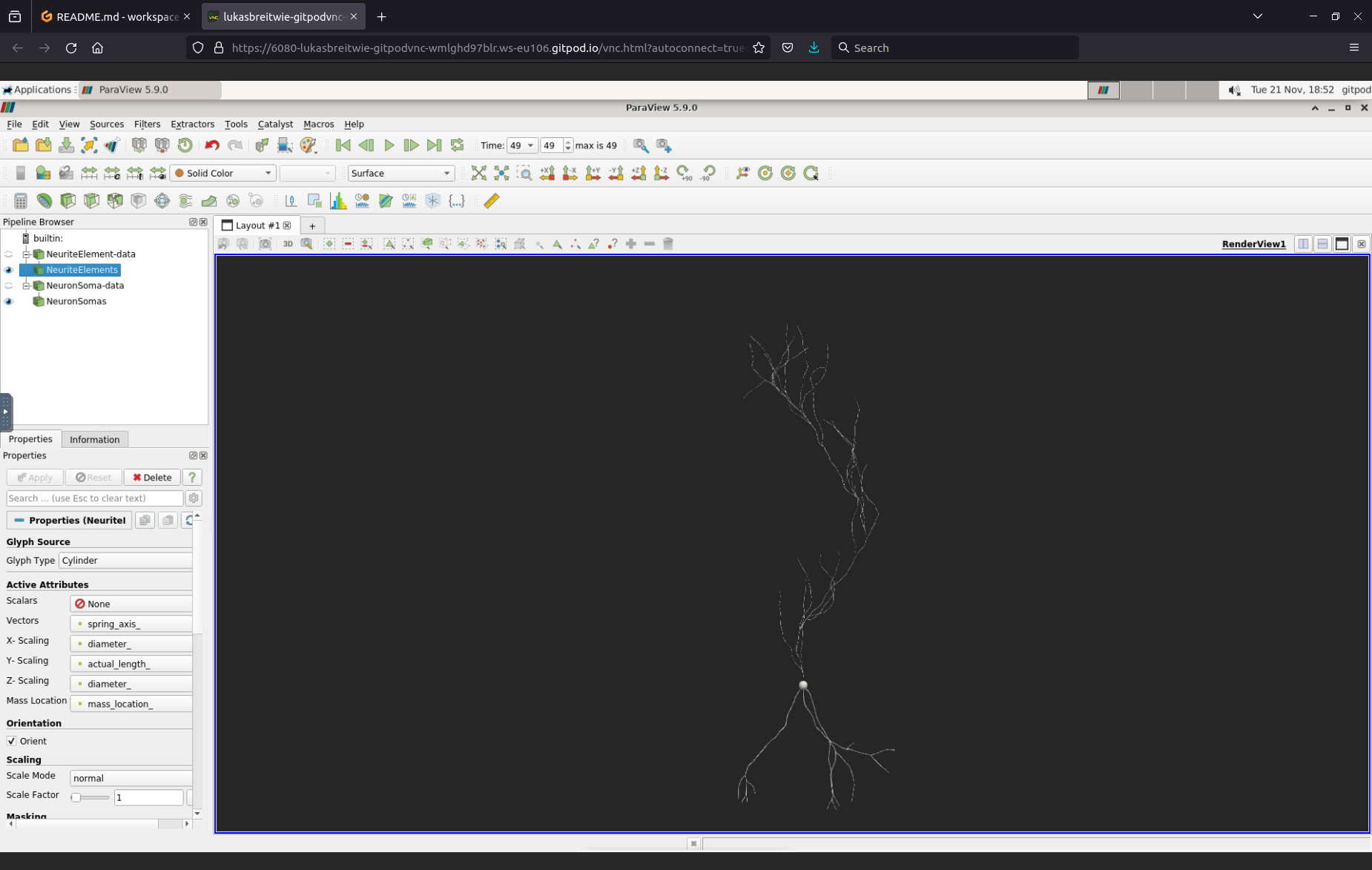
?figurename? 4.8: Full ParaView instance in the web browser using a VNC connection.

Gitpod also supports GUI applications. Executing ParaView in VSCode’s terminal will open a new browser tab showing the full desktop version of BioDynaMo’s main visualization tool in a VNC window (Figure 4.8). The ParaView command is exactly the same as if one would work on a local laptop or workstation (see last terminal line in Figure 4.7).

4.3.5 Backup and Restore

BioDynaMo uses ROOT [361] to integrate the backup and restore functionality transparently. This allows system failures to occur without losing valuable simulation data. Without any user intervention, all simulation data can be persisted to disk as system-independent binary files, called ROOT files, and restored into memory after a failure occurs. The ROOT file format is well-established and is the primary format for storing large quantities (exabyte) of data in high-energy physics experiments, such as CERN. To enable the backup and restore feature in BioDynaMo, one must simply specify the file name of the backup file. Additionally, one can set the interval at which a backup is performed. A low interval value ensures a low amount of data loss whenever a failure occurs, but also increases the incurred overhead for creating the backup files. The advised backup interval depends on the duration of the simulation.

4.3.6 Software Quality Assurance

Compromising on software quality can have severe consequences that can culminate in the retraction of published manuscripts [181]. Therefore, we put tremendous effort into establishing a rigorous development workflow that follows industry best practices. Test-driven development—a practice from agile development [173]—is at the core of our solution. BioDynaMo has over 600 tests distributed among unit, convergence, system, and installation tests. We monitor test coverage of our unit tests with the tool kcov [396], and currently cover 79.8% lines of code. Figure 4.9, for example, shows the convergence test for extracellular diffusion. By comparing the computed results with the analytical solution we observe an increasing accuracy of the diffusion solver when we increase the diffusion grid’s resolution. For each change to our repository (https://github.com/BioDynaMo/biodynamo), GitHub Actions (https://github.com/features/actions) executes the entire test suite and, upon success, updates the documentation on our website. Installation tests are executed on each supported operating system and ensure that all demo simulations run on a default system.

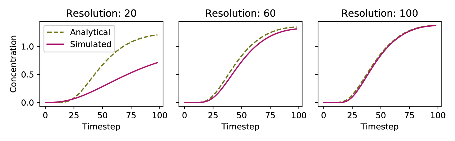
?figurename? 4.9: Diffusion convergence test. The simulated diffusion results converge towards the analytical solution as we increase the resolution of the diffusion grid. The resolution represents the number of grid points in the diffusion grid along each dimension of the simulation space. We use an instantaneous point source at the origin and measure the concentration change over time at $\sqrt{1000}$ micron away from the point source.

Coding Style Guide.

A coding style guide is a set of guidelines and best practices that improve the readability and maintainability of a codebase. Consistency helps new developers and users quickly understand BioDynaMo’s code base. We are using clang-format, clang-tidy, and cpplint to monitor compliance with our style guide. These tools are integrated into our build system and GitHub Actions to provide quick feedback to developers and code reviewers.

4.4 High-Level Features

The high-level layer (Figure 4.2) provides general functionality which is commonly required in agent-based models across many fields.

4.4.1 Generation of Agent Populations

The first step in an agent-based model is to specify the starting condition of the simulation. Therefore, BioDynaMo provides functionality to create agent populations with specific properties. Class ModelInitializer provides several functions to create agents in 3D space (Figure 4.13) and to initialize extracellular substances (Figure 4.3 and Section 4.5.2). Furthermore, to initialize the attributes of an agent population, researchers can use one of the many predefined random number generators that draw samples from a specific distribution (uniform, exponential, gaussian, binomial, etc.) or define their own one. These features are demonstrated in Supplementary Tutorial LABEL:ap:st01, LABEL:ap:st02 and LABEL:ap:st08.

auto create_agent = [](const Real3 position) auto* agent = new SphericalAgent(position); agent->SetDiameter(10); return agent; ; uint64_t num_agents = 300;

(a) Common code

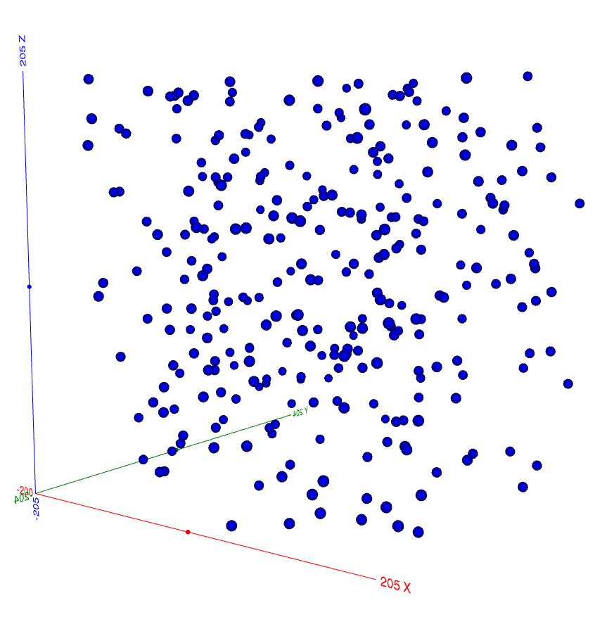
ModelInitializer::CreateAgentsRandom(-200, 200, num_agents, create_agent);

(b) Create agents randomly inside a 3D cube.

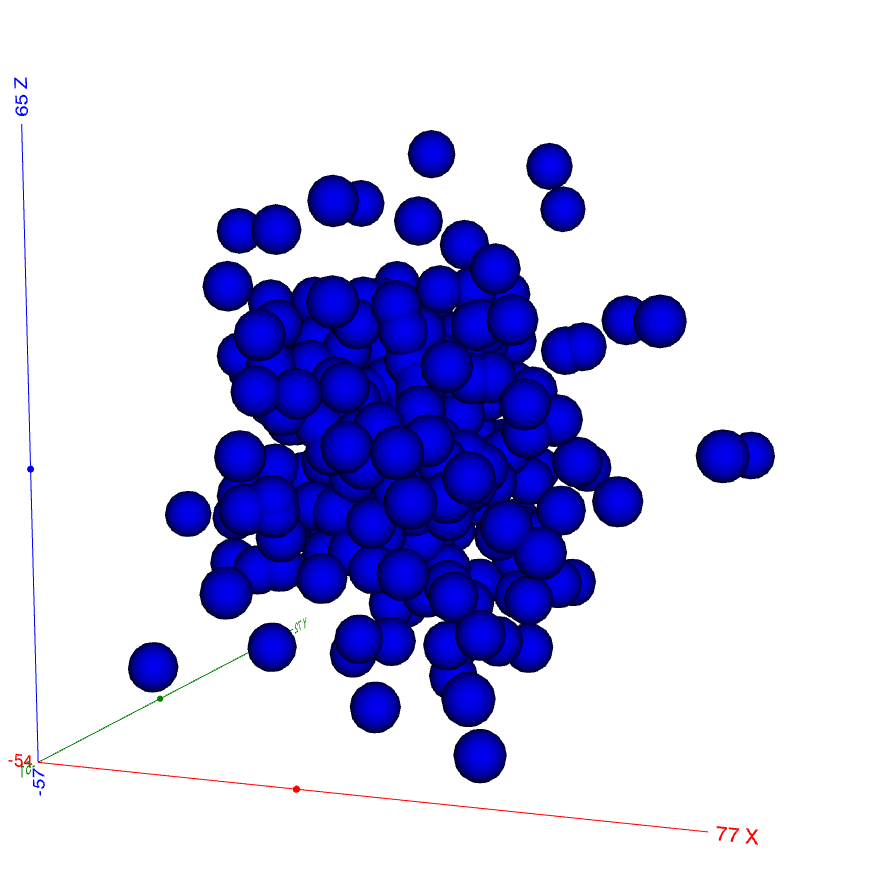
auto rng = simulation.GetRandom()->GetGausRng(0, 20); ModelInitializer::CreateAgentsRandom(-200, 200, num_agents, create_agent, rng);

(c) Create agents randomly inside a 3D cube using a gaussian distribution.

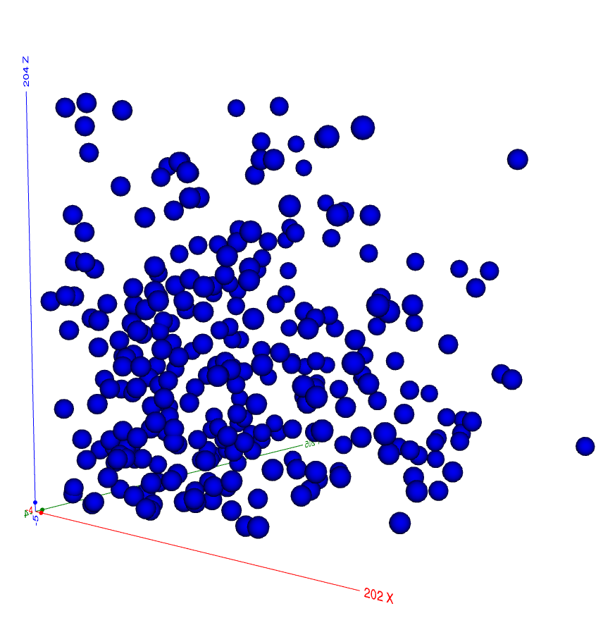
auto rng = simulation.GetRandom()->GetExpRng(100); ModelInitializer::CreateAgentsRandom(-200, 200, num_agents, create_agent, rng);

(a) Create agents randomly inside a 3D cube using an exponential distribution.

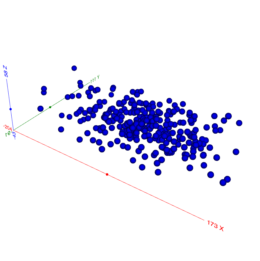
auto gaus3d = [](const real_t* x, const real_t* params) auto mx = params[0]; auto my = params[2]; auto mz = params[4]; auto sx = params[1]; auto sy = params[3]; auto sz = params[5]; auto ret = (1.0 / (sx * sy * sz * std::pow(2.0 * Math::kPi, 3.0 / 2.0))) * std::exp(-std::pow(x[0] - mx, 2.0) / std::pow(sx, 2.0) - std::pow(x[1] - my, 2.0) / std::pow(sy, 2.0) - std::pow(x[2] - mz, 2.0) / std::pow(sz, 2.0)); return ret; ; auto* random = simulation.GetRandom(); auto rng = random->GetUserDefinedDistRng3D(gaus3d, 0, 100, 0, 50, 0, 20, -200, 200, -200, 200, -200, 200); ModelInitializer::CreateAgentsRandom(-200, 200, num_agents, create_agent, rng);

(b) Create agents randomly inside a 3D cube using a 3D gaussian distribution.

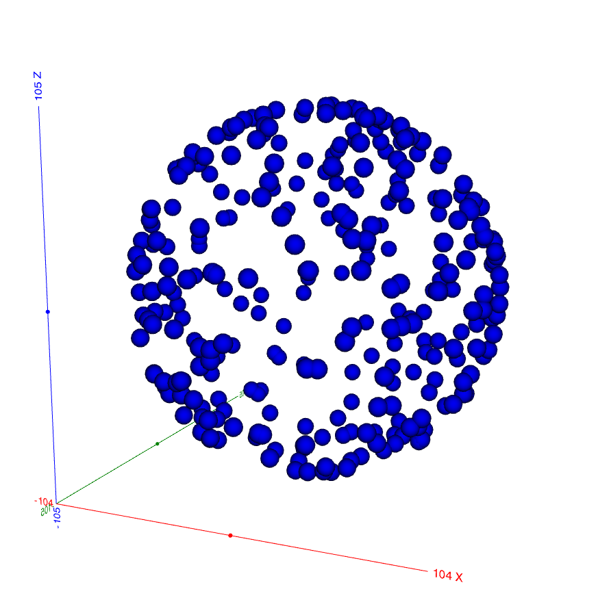
ModelInitializer::CreateAgentsOnSphereRndm(0, 0, 0, 100, num_agents, create_agent);

(a) Create agents randomly on a sphere

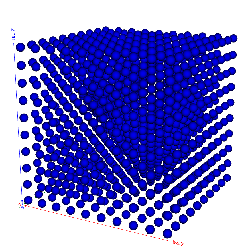
uint64_t agents_per_dim = 10; real_t space_between_agents = 20; ModelInitializer::Grid3D(agents_per_dim, space_between_agents, create_agent);

(b) Create agents on a 3D grid.

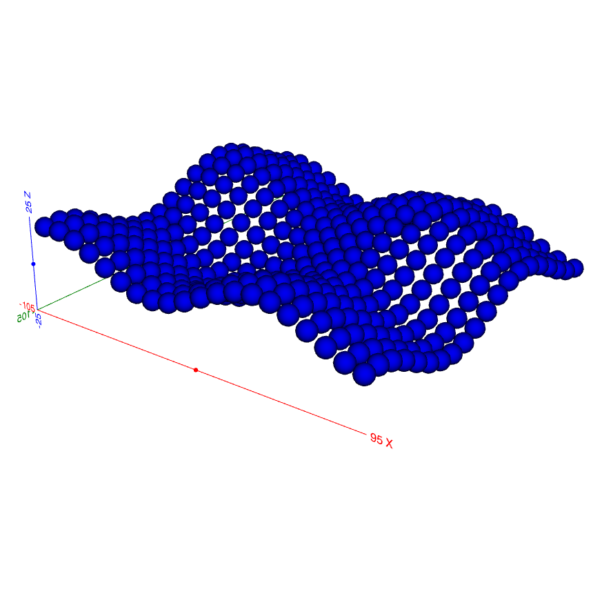
auto f = [](const real_t* x, const real_t* params) return 10 * std::sin(x[0] / 20.) + 10 * std::sin(x[1] / 20.0); ; ModelInitializer::CreateAgentsOnSurface(f, , -100, 100, 10, -100, 100, 10, create_agent);

(a) Create agents on a surface.

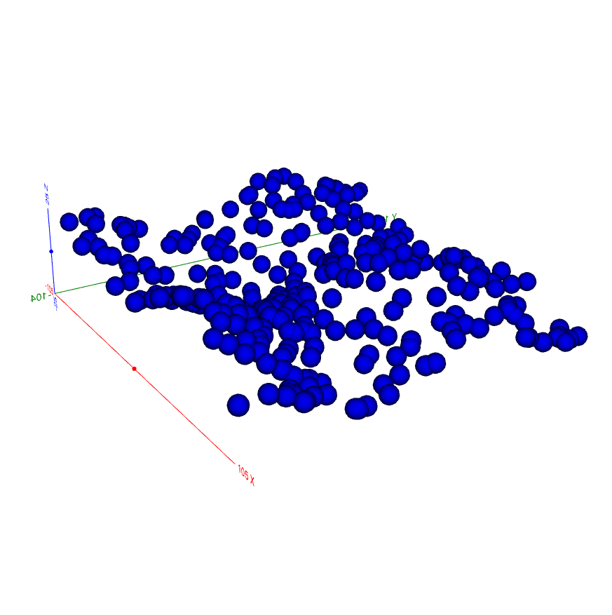
auto f = [](const real_t* x, const real_t* params) return 10 * std::sin(x[0] / 20.) + 10 * std::sin(x[1] / 20.0); ; ModelInitializer::CreateAgentsOnSurfaceRndm(f, , -100, 100, -100, 100, num_agents, create_agent);

(b) Create agents on a surface randomly.

?figurename? 4.13: Generation of agent populations in 3D space. The full tutorial can be found at LABEL:ap:st01.

4.4.2 Agent Reproduction and Mortality

The addition and removal of agents during the execution of a simulation is an integral part of agent-based simulations. Therefore, BioDynaMo provides a framework to create new agents during a simulation and initialize their attributes. By default, agents that are created in iteration i will be visible to other agents in iteration i + 1. The removal of agents is handled identically. The handling of when new or removed agents become visible to the simulation is encapsulated in the execution context. Therefore, a user could provide another implementation where agents are visible immediately.

Besides adding and removing agents, a second major part is to provide a generic way to initialize the attributes of an agent. To this end, BioDynaMo simplifies the regulation of behaviors if new agents are created. The user can control whether a behavior will be copied to a new agent or removed from the existing agent, based on the underlying process (e.g. cell division). Similarly, agents and behaviors have a function Initialize which can be overridden by user-defined agents to initialize additional attributes. These concepts are shown in Figure 4.14 and demonstrated in Supplementary Tutorial LABEL:ap:st03–LABEL:ap:st05.

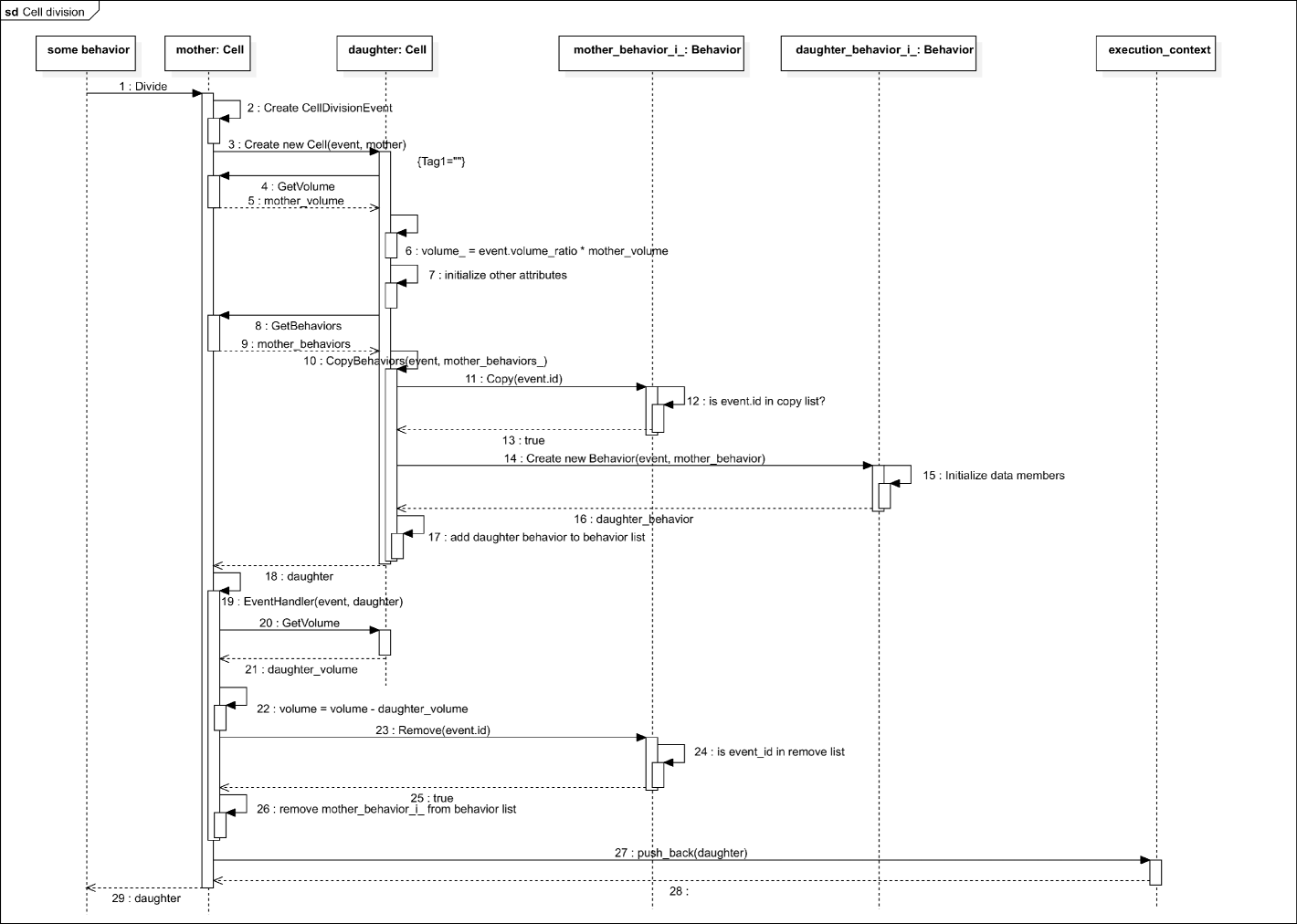
?figurename? 4.14: Event Sequence Diagram.

4.4.3 Environment Search

To determine the agents in the local environment (neighbors), BioDynaMo uses an environment search algorithm (Supplementary Tutorial LABEL:ap:st06). BioDynaMo’s default environment algorithm is based on a uniform grid implementation. The implementation divides the total simulation space into uniform boxes of the same size and assigns agents to boxes based on the center of mass of the agent. Hence, the agents in the environment can be obtained by iterating over the assigned box and all its surrounding boxes (27 boxes in total). The box size is chosen by the user or determined automatically based on the largest agent in the simulation to ensure all mechanical interactions are taken into account. Alternatively, BioDynaMo provides an octree and kd-tree environment implementation. The interface is kept generic enough to support non-euclidean space environment definitions.

4.4.4 Multi-Scale Simulations

A biological simulation has to account for dynamic mechanisms that range from milliseconds to weeks (e.g. physical forces, reaction-diffusion processes, gene regulatory dynamics, etc.). BioDynaMo supports processes at different time scales by providing a parameter to specify the time interval between two time steps and an execution frequency for each operation (Supplementary Tutorial LABEL:ap:st07). An execution frequency of one means that the corresponding operation is executed every time step. In contrast, a frequency of three would mean that the operation is executed every three time steps. This mechanism allows BioDynaMo to simulate e.g. substance diffusion and neurite growth in the same model.

4.4.5 Statistical Analysis

Statistical analysis plays a fundamental role in generating new insights from simulation data. BioDynaMo builds upon the rich features of CERN’s primary data analysis framework ROOT [361], which provides an extensive mathematical, histogram, graphing, and fitting library. BioDynaMo complements this functionality by providing an easy mechanism to collect simulation data over time and a simplified API targeted to the agent-based use case. These capabilities are demonstrated in Supplementary Tutorial LABEL:ap:st08–LABEL:ap:st11.

4.4.6 Hierarchical Model Support

[397] describe an agent-based model in which large agents have to be executed before smaller agents. BioDynaMo supports these hierarchical models with several functions in the ResourceManager, Scheduler, and Operation class. The described order can be implemented in BioDynaMo by adding three lines of code as demonstrated in Supplementary Tutorial LABEL:ap:st12. Additionally, it is possible to execute a different set of operations for large and small agents.

4.4.7 Hybrid Modeling Support

Some models benefit from the combination of multiple simulation methodologies—e.g. the combination of an agent-based and continuum-based model. BioDynaMo’s flexible build system supports hybrid modeling capabilities and was demonstrated by [8] to investigate cancer development.

4.4.8 Dynamic Scheduling

In BioDynaMo the code that will be executed is controlled by behaviors and operations. Behaviors can be attached to individual agents and thus allow very fine-grained control. Agent operations are usually executed for all agents (if no agent filters are specified). Both behaviors and operations can be created, added, removed, and destroyed during a simulation. This feature gives the user maximum flexibility to change the executed simulation code over time (Supplementary Tutorial LABEL:ap:st13).

4.4.9 Parameter Management

BioDynaMo simplifies the definition of simulation parameters by liberating the user from the burden to write code to parse parameter files or command line arguments.

4.4.10 Parameter Optimization

The epidemiology use case presented in the Section 4.6.3 demonstrates how to define an experiment comprised of multiple input parameters, and a user-defined error function. This experiment definition is used in conjunction with the optimlib library (https://www.kthohr.com/optimlib.html) to determine model parameters that match the ground truth.

4.4.11 Space Boundary Conditions

BioDynaMo support three boundary conditions: (i) open, where the simulation space grows to encapsulate all agents in the simulation, (ii) closed, where artificial walls prevent agents from exiting the simulation space, and (iii) toroidal, where agents that leave the space on one side, will enter on the opposite side.

4.5 Model Building Blocks

Currently, BioDynaMo’s building blocks (Figure 4.2) belong to the (neural) tissue modeling domain. Similar to the biological model presented in [39], BioDynaMo supports spherical and cylindrical agent geometries, mechanical interactions between agents, and diffusion of extracellular substances.

With these features, researchers can simulate cell body dynamics, neural growth, and gene regulatory networks.

Simulations to study the development of (neural) tissue are only one example of how BioDynaMo could be used in the future. By designing BioDynaMo in a modular and extensible way, we laid the foundation to create new building blocks easily (Figure 4.3 and Section 4.6.3). Supplementary Tutorial LABEL:ap:st15 for example demonstrates how to replace the default mechanical force implementation with a user-defined one.

Table LABEL:tab:biological-features lists the agents, behaviors, and operations that the BioDynaMo v1.0 installation contains.

4.5.1 Mechanical Forces

Growing realistic cell and tissue morphologies requires the consideration of mechanical interactions between agents. Therefore, BioDynaMo examines if two agents collide with each other at every timestep. To find all possible collisions, it is sufficient to evaluate neighbors in the environment. Whenever two agents (e.g. a cell body or a neurite element) overlap, a collision occurs. If a collision is detected, the engine calculates the mechanical forces that act on them.

The mechanical force calculation between spheres and cylinders follows the same approach as the implementation in Cortex3D [39]. Both in BioDynaMo and Cortex3D, the magnitude of the force is computed based on [398] and comprises a repulsive and attractive component:

$$\begin{aligned} F_{N}=k\delta-\gamma\sqrt{r\delta}\end{aligned}$$ (4.1)

where $\delta$ indicates the spatial overlap between the two elements, and $r$ denotes a combined measure of the two radii:

$$\begin{aligned} r=\frac{r_{1}r_{2}}{r_{1}+r_{2}}\end{aligned}$$ (4.2)

where the radii denote the radii of the interacting spheres or cylinder.

Eq 4.1 comprises the effects of the structural tension from the pressure between the colliding membrane segments, and the attractive force due to the cell adhesion molecules. The magnitudes of these two force components depend upon the modifiable parameters $k$ and $\gamma$. In the current form, as in Cortex3D, these are set to $2$ and $1$, respectively. After the forces have been determined, the agents change their 3D location depending on the force resulting from all the mechanical interactions with neighbors. More details about the implementation of the mechanical force, including the force between neighboring neurite elements, can be found in [39].

4.5.2 Extracellular Diffusion

Signaling molecules, which differentiate and regulate cells, reach their destination through diffusion [399]. A well-studied example of this process, called morphogen gradients, is the determination of vein positions in the wing of Drosophila [400].

BioDynaMo solves the partial differential equations that model the diffusion of extracellular substances (Fick’s second law) with the discrete central difference scheme [401]. A grid is imposed on the simulation space, and at each timestep, the concentration value of each grid point is updated according to

$$\begin{aligned} u_{i,j,k}^{n+1}=u_{i,j,k}^{n}\times(1-\mu*\Delta t)&+\frac{\nu\Delta t}{\Delta x^{2}}(u_{i+1,j,k}^{n}-2u_{i,j,k}^{n}+u_{i-1,j,k}^{n})\\ &+\frac{\nu\Delta t}{\Delta y^{2}}(u_{i,j+1,k}^{n}-2u_{i,j,k}^{n}+u_{i,j-1,k}^{n})\\ &+\frac{\nu\Delta t}{\Delta z^{2}}(u_{i,j,k+1}^{n}-2u_{i,j,k}^{n}+u_{i,j,k-1}^{n})\,,\end{aligned}$$ (4.3)

where $u_{i,j,k}^{n}$ is the concentration value on grid point $(i,j,k)$ at timestep $n$, $\nu$ is the diffusion coefficient, $\mu$ is the decay constant, $\Delta t$ is the duration of one timestep, and $\Delta x$, $\Delta y$, and $\Delta z$ are the distances between grid points in the x, y, and z direction, respectively. The distances between the grid points are inversely proportional to the resolution and determine the accuracy of the solver.

In BioDynaMo, it is possible to define the diffusion behavior at the simulation boundaries. In the default implementation, which we use for our examples in the result section, substances diffuse out of the simulation space.

BioDynaMo provides predefined substance initializers (e.g., Gaussian) and accepts user-defined functions for arbitrary distributions to determine the initial concentration values. We used this functionality, for example, in the pyramidal cell growth simulation.

4.5.3 Systems Biology Markup Language Integration

Systems biology markup language (SBML) is a well-established standard to describe chemical reaction networks to model metabolism, or cell signaling [402]. The BioModels database contains a collection of more than 9000 models in this format [403].

Therefore, BioDynaMo provides the possibility to simulate chemical reaction networks described as SBML [402] models (Figure 4.15). BioDynaMo uses libroadrunner [404] to solve the reaction equations, which features various deterministic and stochastic solvers. The intracellular concentration of substances can serve as a control mechanism for agent behaviors displacement, division, branching, etc. Furthermore, it is feasible to couple the intracellular domain with the extracellular matrix by exocytosis and endocytosis of substances and extracellular diffusion.

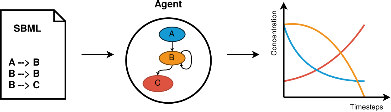
?figurename? 4.15: SBML integration. Chemical reaction networks defined in SBML format can be loaded into BioDynaMo and assigned to any agent. The reaction equations are solved for each timestep.

4.6 Exemplary Use Cases

We demonstrate BioDynaMo’s capacity to simulate disparate problems in systems biology with simple yet representative use cases in neuroscience, oncology, and epidemiology. Since BioDynaMo does not contain any epidemiological building blocks, this use case indicates how easy it is to implement a model based solely on features from the high- and low-level layer (Figure 4.2).

For each use case we present the implemented model, validate the simulation results against verified experimental or analytical data, and report performance data for different problem sizes on multiple hardware configurations. Furthermore, we provide pseudocode for all agent behaviors and a table with model parameters.

4.6.1 Neuroscience Use Case

This example illustrates the use of BioDynaMo to model neurite growth of pyramidal cells using chemical cues. Initially, a pyramidal cell, composed of a 10 $\mu m$ cell body, three 0.5 $\mu m$ long basal dendrites, and one 0.5 $\mu m$ long apical dendrite (all of them considered here as agents), is created in 3D space (L37–L51). Furthermore, two artificial growth factors were initialized, following a Gaussian distribution along the z-axis (L54–L65). The distribution of these growth factors guided dendrite growth and remained unchanged during the simulation.

[fontsize=]neuroscience-example.cc

Listing 1: Pyramidal cell growth simulation code. This example shows the required C++ code to simulate the growth of a single pyramidal cell as shown in Figure 4.16A. All classes and functions which are not defined in this example are provided by BioDynaMo. Only the body of the two behavior’s Run methods has been ommited, but are provided in Supplementary File S3 (SF3-code.tar.gz) and Algorithm 1.

Dendritic development was dictated by a behavior defining growth direction, speed, and branching behavior for apical and basal dendrites (L12–L35, see also Algorithm 1).

1

2

input : neurite, growth_factor, diameter_threshold, diameter_threshold_two, growth_speed, branching_probability, old_direction_weight, randomness_weight, gradient_weight, shrinkage, can_branch

3

4diameter $\leftarrow$ neurite.GetDiameter();

5 if $\textnormal{{diameter}}>\textnormal{{diameter\_threshold}}$ then

6    old_direction $\leftarrow$ neurite.GetDirection();

7    pos $\leftarrow$ neurite.GetPosition();

8    gradient $\leftarrow$ growth_factor.GetNormalizedGradient(pos);

9    direction $\leftarrow$ $\textnormal{{old\_direction}}\times\textnormal{{old\_direction\_weight}}+\textnormal{{gradient}}\times\textnormal{{gradient\_weight}}+\textnormal{{RandomUniform3(}}\textnormal{\emph{-1, 1}}\textnormal{{)}}\times\textnormal{{randomness\_weight}}$;

10    neurite.Extend(growth_speed, direction);

11    neurite.SetDiameter(diameter- shrinkage);

12    if neurite.IsApical() then

13       if can_branch and neurite.IsTerminal() and $\textnormal{{diameter}}<\textnormal{{diameter\_threshold\_two}}$ and $\textnormal{{RandomUniform(}}\textnormal{\emph{0, 1}}\textnormal{{)}}<\textnormal{{branching\_probability}}$ then

14          branching_direction $\leftarrow$ CalculateBranchingDirection(neurite);

15          neurite.Branch(branching_direction);

16         

17       end if

18      

19    end if

20   else if $\textnormal{{RandomUniform(}}\textnormal{\emph{0, 1}}\textnormal{{)}}<\textnormal{{branching\_probability}}$ then

21       neurite.Bifurcate();

22      

23    end if

24   

25 end if

Algorithm 1 Apical and basal dendrite growth.

At each step of the simulation, the dendritic growth direction depended on the local chemical growth factor gradient, the dendrite’s previous direction, and a randomly chosen direction. In addition, the dendrite’s diameter tapered as it grew (shrinkage), until it reached a specified diameter, preventing it from growing any further. The weight of each element on the direction varied between apical and basal dendrites.

These simple rules gave rise to a straight long apical dendrite with a simple branching pattern and more dispersed basal dendrites, as shown in Figure 4.16A, similar to what can be observed in real pyramidal cell morphologies as shown in Figure 4.16B or [405] (Figure 1A CA1). Using our growth model, we were able to generate a large number of various realistic pyramidal cell morphologies. We used a publicly available database of real pyramidal cells coming from [5] for comparison and parameter tuning. Table 4.1 shows the determined parameters. Two measures were used to compare our simulated neurons and the 69 neurons composing the real morphologies database: the average number of branching points, and the average length of dendritic trees. No significant differences were observed between our simulated neurons and the real ones ($p<0.001$ using a T-test for two independent samples). These results are shown in Figure 4.16D. The model specification of the pyramidal cell growth simulation consists of 127 lines of C++ code (Listing 1).

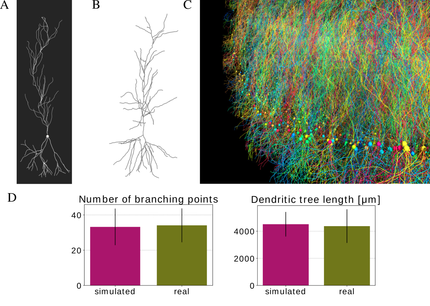
?figurename? 4.16: Pyramidal cell simulation. (A) Example pyramidal cell simulated with BioDynaMo. (B) Real neuron (R67nr67b-CEL1.CNG) taken from [5] and visualized with https://neuroinformatics.nl/HBP/morphology-viewer/ (C) Large-scale simulation. The model started with 5000 initial pyramidal cell bodies and contained 9 million agents after simulating 500 iterations. The simulation execution time was 35 seconds on a server with 72 CPU cores. (D) Morphology comparison between simulated neurons and experimental data from [5]. Error bars represent the standard deviation. (A,C) A video is available in the Supplementary Information.

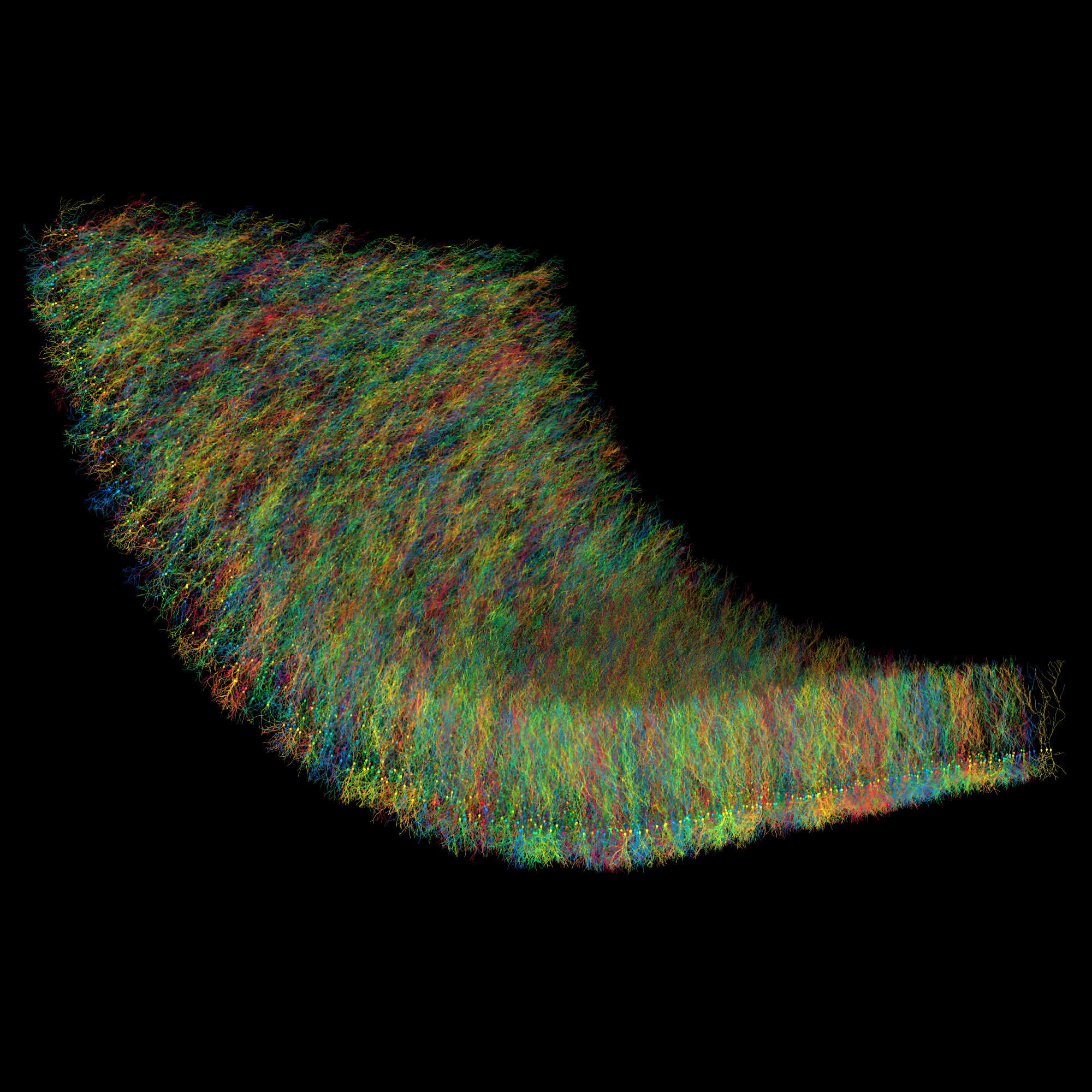
?figurename? 4.17: Large-scale pyramidal cell simulation. The model started with 5000 initial pyramidal cell bodies and contained 9 million agents after simulating 500 iterations. The simulation execution time was 35 seconds on a server with 72 CPU cores. A video is available in the Supplementary Information.

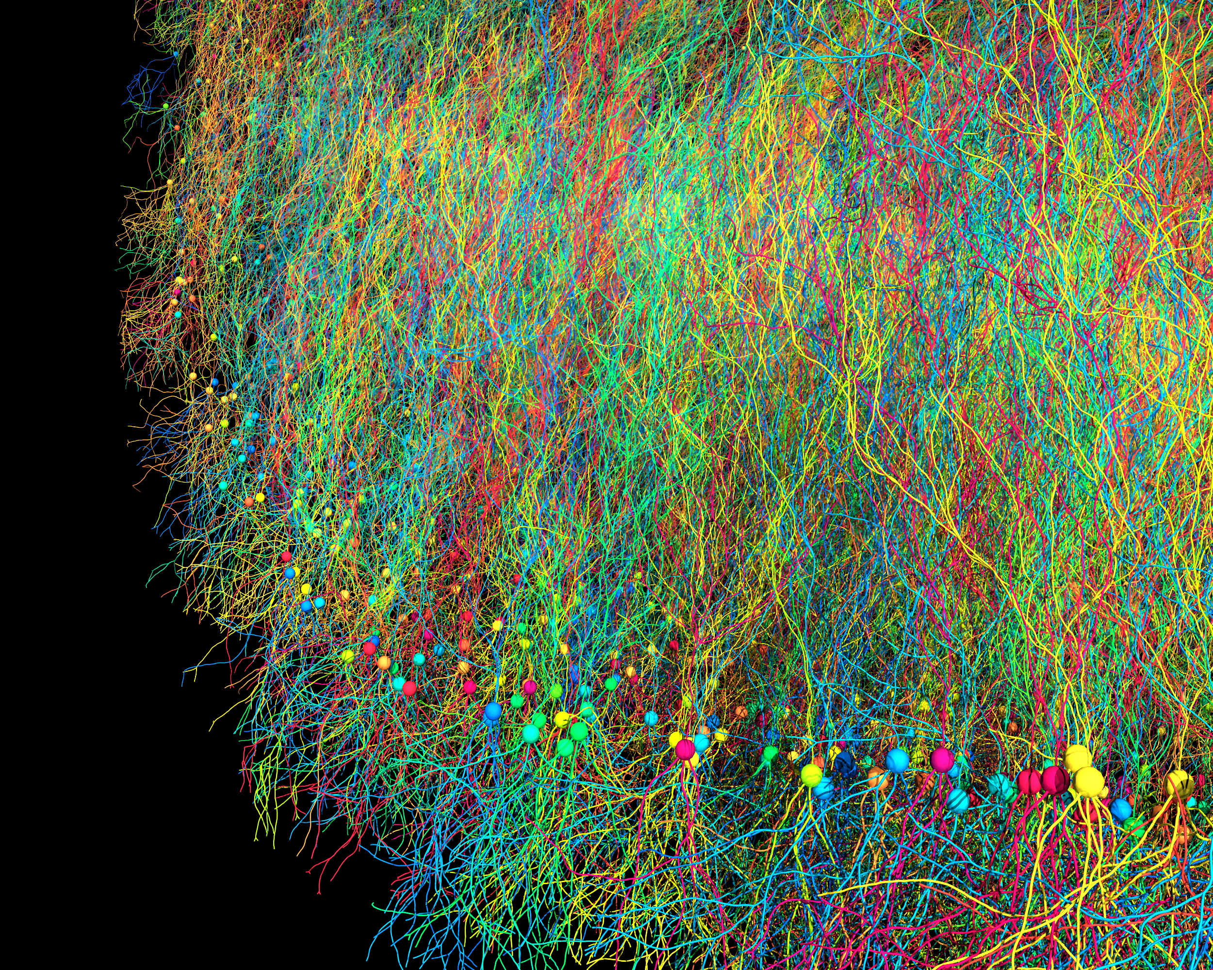
?figurename? 4.18: Large-scale pyramidal cell simulation. Detailed view of the simulation shown in Figure 4.17.

?tablename? 4.1: Model parameters for the pyramidal cell growth simulation.

Parameter	Apical dendrite	Basal dendrite
Diameter threshold	$0.575$	$0.75$
Diameter threshold two	$0.55$
Old direction weight	$4$	$6$
Gradient weight	$0.06$	$0.03$
Randomness weight	$0.3$	$0.4$
Growth speed	$100$	$50$
Shrinkage	$0.00071$	$0.00085$
Branching probability	$0.038$	$0.006$

Figure 4.16C, 4.17, and 4.18 show a large-scale simulation incorporating 5000 neurons similar to the one described above and demonstrates the potential of BioDynaMo for developmental, anatomical, and connectivity studies in the brain. This simulation contained 9 million agents.

4.6.2 Oncology Use Case

In this section, we present a tumor spheroid simulation to replicate in vitro experiments from [6]. Tumor spheroid experiments are typically employed to investigate the pathophysiology of cancer and are also being used for pre-clinical drug screening [406]. Here we considered three in vitro test cases using a breast adenocarcinoma MCF-7 cell line [6] with different initial cell populations ($2000$, $4000$, and $8000$ MCF-7 cells). Our goal was to simulate the growth of this mono cell culture embedded in a collagenous (extracellular) matrix.

The fundamental cellular mechanisms modeled here include cell growth, cell duplication, cell migration, and cell apoptosis. All these processes are implemented in the class TumorCellBehavior (see Algorithm 2). The cell growth rate was derived from the published data [407], while cell migration (cell movement speed), cell survival, and apoptosis were fine-tuned after trial and error testing (see Table 4.2). Since the in vitro study considered the same agarose gel matrix composition among the experiments, the BioDynaMo model assumes identical parameters for the cell–matrix interactions in the simulations. Considering the homogeneous ECM properties, tumor cell migration was modeled as Brownian motion.

1

2

3

input : cell, minimum_cell_age, death_probability, displacement_rate, growth_speed, division_probability

4

5random_vector $\leftarrow$ RandomUniform3(-1, 1);

6 brownian $\leftarrow$ $\textnormal{{random\_vector}}\div\textnormal{{random\_vector}}.\textnormal{{L2Norm(}}\textnormal{\emph{}}\textnormal{{)}}$;

7 cell.UpdatePosition($\textnormal{{brownian}}\times\textnormal{{displacement\_rate}}$);

8

9if $\textnormal{{age}}>=\textnormal{{minimum\_cell\_age}}$ and $\textnormal{{RandomUniform(}}\textnormal{\emph{0, 1}}\textnormal{{)}}<\textnormal{{death\_probability}}$ then

10    cell.RemoveFromSimulation();

11    return ;

12   

13 end if

14age $\leftarrow\textnormal{{age}}+1$;

15

16if $\textnormal{{cell}}.\textnormal{{GetDiameter}}<\textnormal{{max\_diameter}}$ then

17    cell.IncreaseVolume(growth_speed);

18   

19 else if $\textnormal{{RandomUniform(}}\textnormal{\emph{0, 1}}\textnormal{{)}}<\textnormal{{division\_probability}}$ then

20    cell.Divide();

21   

22 end if

Algorithm 2 Cancer cell behavior.

?tablename? 4.2: Model parameters for the tumor spheroid growth simulations.

Parameter [dimensions]	2000	4000	8000
	cells/well
Cell growth rate [$\mu$m3/h]	$42.0$	$35.0$	$29.9$
Minimum cell age to apoptosis [h]	$87$	$87$	$87$
Division probability	$0.0215$	$0.0215$	$0.0215$
Cell death probability	$0.033$	$0.033$	$0.033$
Maximum cell speed [$\mu$m/h]	$1.0$	$0.9$	$0.2$
Cell–ECM adherence	$1.8$	$1.8$	$1.8$
coefficient [dimensionless]
Random cell movement	$0.005$	$0.005$	$0.0005$
= displacement rate [$\mu$m/h]

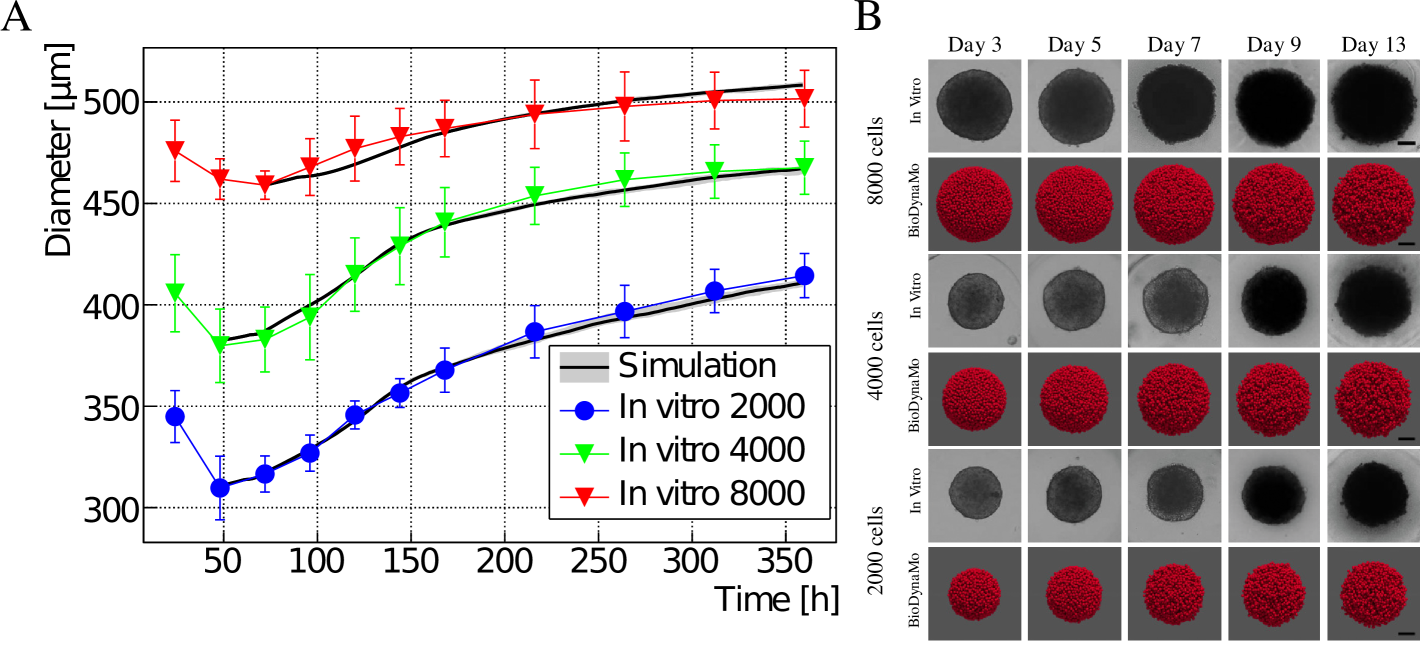
?figurename? 4.19: Comparison between in vitro MCF-7 tumor spheroid experiments and our in silico simulations using BioDynaMo. (A) Human breast adenocarcinoma tumor spheroid (MCF-7 cell line) development during a 15 day period, where different initial cell populations were considered (see Fig 3 in [6]). Error bars denote standard deviation to the experimental data. The mean of the in silico results is shown as a solid black line with a grey band depicting minimum and maximum observed value. (B) shows a qualitative comparison between the microscopy images and simulation snapshots. Scale bars correspond to 100$\mu$m. A video is available in the Supplementary Information.

The in vitro experiments from [6] and the simulations using BioDynaMo are depicted in Figure 4.19. Each line plot in Figure 4.19A compares the mean diameter between the experiments and the simulations over time, which demonstrates the validity and accuracy of BioDynaMo. The diameter of the spheroids in the simulations were deducted from the volume of the convex hull that enclosed all cancer cells. The in vitro experiments used microscopy imaging to measure the spheroid’s diameters [6]. Figure 4.19B compares snapshots of the simulated tumor spheroids (bottom row) against microscopy images of in vitro spheroids (top row) at different time points. The spheroid’s morphologies between the in vitro experiments and the BioDynaMo simulations are in excellent agreement.

Model specification required 154 lines of C++ code.

4.6.3 Epidemiology Use Case

This section presents an agent-based model that describes the spreading of infectious diseases between humans. The model divides the population into three groups: susceptible, infected, and recovered (SIR) agents. We compare our simulation results with the solution of the original SIR model from [216], which used the following three differential equations to describe the model dynamics: $dS/dt=-\beta SI/N$, $dI/dt=\beta SI/N-\gamma I$, and $dR/dt=\gamma I$. $S$, $I$, and $R$ are the number of susceptible, infected, and recovered individuals, $N$ is the total number of individuals, $\beta$ is the mean transmission rate, and $\gamma$ is the recovery rate.

For our agent-based implementation (Figure 4.20C) we created a new agent (representing a person) that encompasses three new behaviors (see Figure 4.3). A susceptible agent became infected with the infection probability if an infected agent was within the infection radius (Algorithm 3). An infected agent recovered with the recovery probability at every time step (Algorithm 4). All agents moved randomly in space with toroidal boundary condition. The absolute distance an agent may travel in every time step was limited (Algorithm 5).

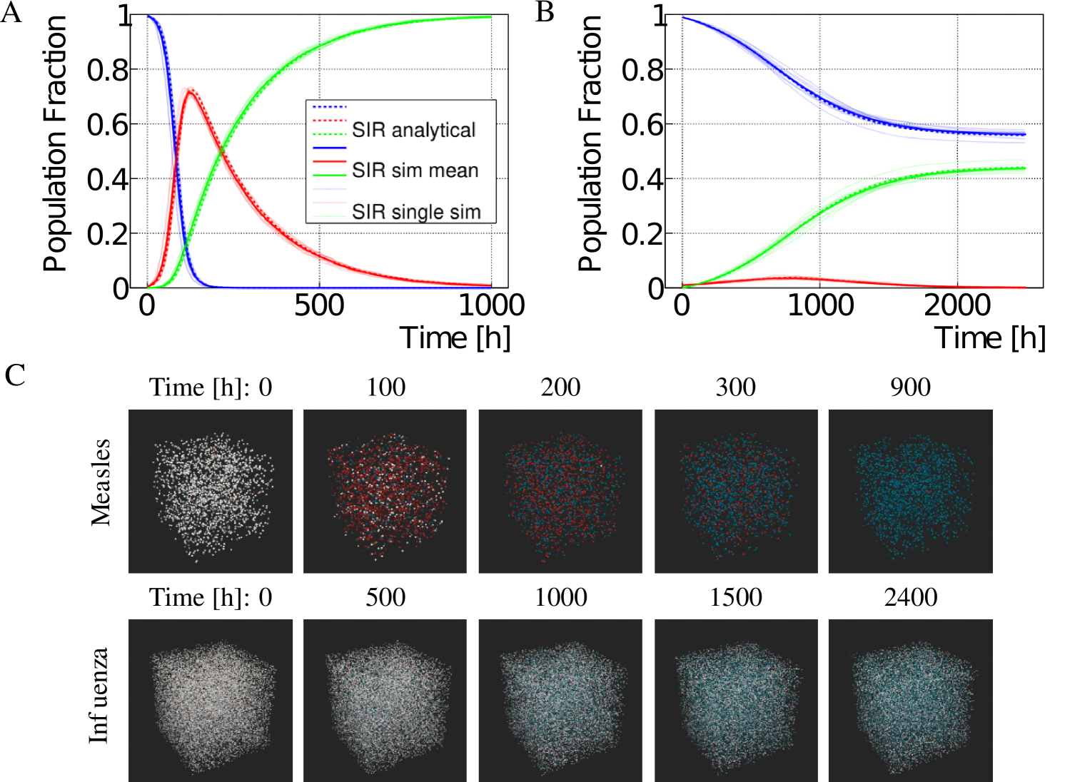
?figurename? 4.20: Measles and seasonal influenza SIR model results. (A,B) Comparison between agent-based (solid lines) and analytical (dashed lines) model for measles (A) and seasonal influenza (B). The agent-based simulation was repeated ten times. The individual simulation results are shown as thin solid lines. The bold solid line represents the mean from all simulations. The legend is shared between the two plots. (C) Visualization of the measles and influenza model for different time steps in 3D space. Susceptible persons are shown in white, infected persons in red, and recovered persons in blue.

1

2

3

input : person, environment, infection_probability, infection_radius

4

5if $\textnormal{{person}}.\textnormal{{GetState(}}\textnormal{\emph{}}\textnormal{{)}}==\textnormal{{susceptible}}$ and $\textnormal{{RandomUniform(}}\textnormal{\emph{0,1}}\textnormal{{)}}<\textnormal{{infection\_probability}}$ then

6    neighbors $\leftarrow\textnormal{{environment}}.\textnormal{{GetNeighbors(}}\textnormal{\emph{{{infection\_radius}}}}\textnormal{{)}}$;

7    for each neighbor in neighbors do

8       if $\textnormal{{neighbor}}.\textnormal{{GetState(}}\textnormal{\emph{}}\textnormal{{)}}==\textnormal{{infected}}$ then

9          person.SetState(infected);

10         

11       end if

12      

13    end for

14   

15 end if

Algorithm 3 Infection behavior.

1

2

3

input : person, recovery_probability

4

5if $\textnormal{{person}}.\textnormal{{GetState(}}\textnormal{\emph{}}\textnormal{{)}}==\textnormal{{infected}}$ and $\textnormal{{RandomUniform(}}\textnormal{\emph{0,1}}\textnormal{{)}}<\textnormal{{recovery\_probability}}$ then

6    person.SetState(recovered);

7   

8 end if

Algorithm 4 Recovery behavior.

1

2

3

input : person, speed, max_bound

4

5position $\leftarrow$ person.GetPosition();

6 movement $\leftarrow$ RandomUniform3(-1, 1).L2Norm();

7 new_position $\leftarrow\textnormal{{position}}+\textnormal{{movement}}\times\textnormal{{speed}}$;

8 for each el in new_position do

9    el $\leftarrow\textnormal{{fMod(}}\textnormal{\emph{{{el}}, {{max\_bound}}}}\textnormal{{)}}$;

10    if $\textnormal{{el}}<0$ then

11       el $\leftarrow\textnormal{{max\_bound}}+\textnormal{{el}}$;

12      

13    end if

14   

15 end for

16person.SetPosition(new_position);

Algorithm 5 Random movement behavior.

We selected two infectious diseases with different characteristics to verify our model: measles and seasonal influenza. We obtained values for the basic reproduction number $R_{0}$ and recovery duration $T_{R}$ from the literature (Measles: $R_{0}=12.9$, $T_{R}=8$ days [408, 307], Influenza: $R_{0}=1.3$, $T_{R}=4.1$ days [409]) and determined the parameters $\beta$ and $\gamma$ for the analytical model, based on $R_{0}=\beta/\gamma$ and $\gamma=1/T_{R}$. For the agent-based model we set the recovery probability to $\gamma$, and determined the remaining parameters (infection radius, infection probability, and maximum movement in one time step) using particle swarm optimization [308] (see Table 4.3). Figure 4.20 shows that the agent-based model is in excellent agreement with the equation-based approach from [216] for measles and influenza.

?tablename? 4.3: Model parameters for the epidemiological use case.

Parameter [dimension]	Measles	Seasonal Influenza
$\beta$ (analytical solution)	$0.06719$	$0.01321$
$\gamma$ (analytical solution)	$0.00521$	$0.01016$
Time step interval [h]	$1$	$1$
Number of time steps	$1000$	$2500$
Cubic simulation space length [m]	$100$	$215$
Initial number of susceptible persons	$2000$	$20000$
Initial number of infected persons	$20$	$200$
Infection radius [m]	$3.24179$	$3.2123$
Infection probability	$0.28510$	$0.04980$
Recovery probability	$0.00521$	$0.01016$
Max movement per time step [m]	$5.78594$	$4.2942$

Model specification required 181 lines of C++ code.

4.6.4 Code Examples

Figure 4.3 depicts in an abstract way that BioDynaMo’s software design is open for extension. With the four code examples in Listing 1 to 4—taken directly from the presented use cases and benchmarks—we want to emphasize how little code is required to add new functionality.

⬇

1struct SimParam : public ParamGroup {

2 BDM_PARAM_GROUP_HEADER(SimParam, 1);

3 uint64_t cells_per_dim = 30;

4 uint64_t iterations = 100;

5};

Listing 2: Additional simulation parameters for the cell growth and division benchmark.

⬇

1/// Possible states.

2enum State { kSusceptible, kInfected, kRecovered };

3

4class Person : public Cell {

5 BDM_AGENT_HEADER(Person, Cell, 1);

6

7 public:

8 Person() {}

9 explicit Person(const Double3& position) : Base(position) {}

10 virtual ~Person() {}

11

12 /// This attribute stores the current state of the person.

13 int state_ = State::kSusceptible;

14};

Listing 3: New agent class used in the epidemiology use case.

⬇

1struct Recovery : public Behavior {

2 BDM_BEHAVIOR_HEADER(Recovery, Behavior, 1);

3

4 Recovery() {}

5

6 void Run(Agent* a) override {

7 auto* person = bdm_static_cast<Person*>(a);

8 if (person->state_ == kInfected) {

9 auto* sim = Simulation::GetActive();

10 auto* random = sim->GetRandom();

11 auto* sparam = sim->GetParam()->Get<SimParam>();

12 if (random->Uniform(0, 1) <= sparam->recovery_probability) {

13 person->state_ = State::kRecovered;

14 }

15 }

16 }

17};

Listing 4: New behavior used in the epidemiology use case.

4.7 Performance Analysis

We compare BioDynaMo’s performance with two established serial ABS platforms (Cortex3D [39] and NetLogo [186]), analyze BioDynaMo’s scalability, and quantify the impact of GPU acceleration. Display updates are turned off on all platforms for these evaluations. Cortex3D has the highest similarity in terms of the underlying biological model out of all the related works presented in Section 3. More specifically, BioDynaMo and Cortex3D use the same method to determine mechanical forces between agents and the same model to grow neural morphologies. This makes Cortex3D the best candidate with which to compare BioDynaMo and ensure a fair comparison.

We quantify the performance of BioDynaMo with four simulations: cell growth and division, soma clustering, pyramidal cell growth, and the epidemiology use case. Table 4.4 details the experimental setup that we used.

System Main memory CPU / GPU OS A 504 GB Server with four Intel(R) Xeon(R) E7-8890 v3 CPUs @ 2.50GHz with a total of 72 physical cores, two threads per core and four NUMA nodes. CentOS 7.9.2009 B 1008 GB C 191 GB Server with two Intel(R) Xeon(R) Gold 6130 CPUs @ 2.10GHz with 16 physical cores, two threads per core, and two NUMA nodes. One NVidia Tesla V100 SXM2 GPU with 32 GB memory. CentOS 7.7.1908 D 16 GB Dell Latitude 7480 Laptop from 2017. One Intel(R) Core(TM) i7-7600U CPU @ 2.80GHz with two physical cores and two threads per core. One Intel HD Graphics 620 GPU with 64 MB eDRAM. Ubuntu 20.04.1 LTS

?tablename? 4.4: Experimental setup. Main parameters of the systems that we used to run the benchmarks of this chapter. SF3-code.tar.gz contains more details.

We compare the runtime of the first three simulations with Cortex3D and the epidemiology use case with NetLogo 3D. These simulations have different properties and are, therefore, well suited to evaluate BioDynaMo’s simulation engine under a broad set of conditions.

4.7.1 Benchmark Simulations

Cell Growth and Division Benchmark.

The starting condition of this simulation was a 3D grid of cells. These cells were programmed to grow to a specific diameter and divide afterward. This simulation had high cell density and slow-moving cells. This simulation covered mechanical interaction between spherical cells, biological behavior, and cell division.

Soma Clustering Benchmark.

The goal of this model was to cluster two types of cells that are initially randomly distributed. These cells are represented in red and blue in Figure 4.21A and B. Each cell type secreted a specific extracellular substance which attracted homotypic cells. Substances diffused through the extracellular matrix following Eq 4.3. We modeled cell processes with two behaviors, ran in sequence: substance secretion (Algorithm 6) and chemotaxis (Algorithm 7). We set the parameter secretion_quantity to $1$ and gradient_weight to $0.75$. During the simulation, cell clusters formed depending on their type. The final simulation state after 6000 time steps is shown in Figure 4.21B. Clusters were associated with non-homogeneous extracellular substance distributions, as shown in Figure 4.21C and Figure 4.22. Besides being used as a benchmark, this example demonstrates the applicability of BioDynaMo for modeling biological systems, including the dynamics of chemicals such as oxygen or growth factors. The simulation consisted of 68 lines of C++ code. Table 4.5 shows the performance on different systems. There are three main differences comparing this simulation with the previous cell growth and division simulation. First, this simulation covered extracellular diffusion. Second, cells moved more rapidly. Third, the number of cells remained constant during the simulation.

1

2

input : cell, diffusion_grid, secretion_quantity

3 pos $\leftarrow$ cell.GetPosition();

4 diffusion_grid.IncreaseConcentrationBy(pos, secretion_quantity);

5

Algorithm 6 Soma clustering substance secretion.

1

2

input : cell, diffusion_grid, gradient_weight

3

4pos $\leftarrow$ cell.GetPosition();

5 grad $\leftarrow$ diffusion_grid.GetNormalizedGradient(pos);

6 cell.UpdatePosition(grad $\times\textnormal{{gradient\_weight}}$);

7

Algorithm 7 Soma clustering chemotaxis.

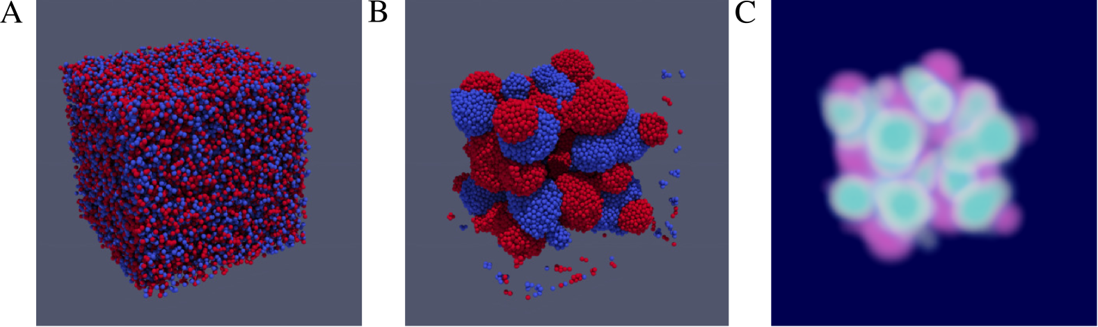
?figurename? 4.21: Soma clustering simulation. This simulation contains two types of cells and two extracellular substances. Each cell secretes a substance and moves into the direction of the substance gradient. Cells are distributed randomly in the beginning (A) and form clusters during the simulation. (B) Cell clusters at the end of the simulation. (C) Substance concentrations at the end of the simulation. A video is available at SV4-soma-clustering.mp4..

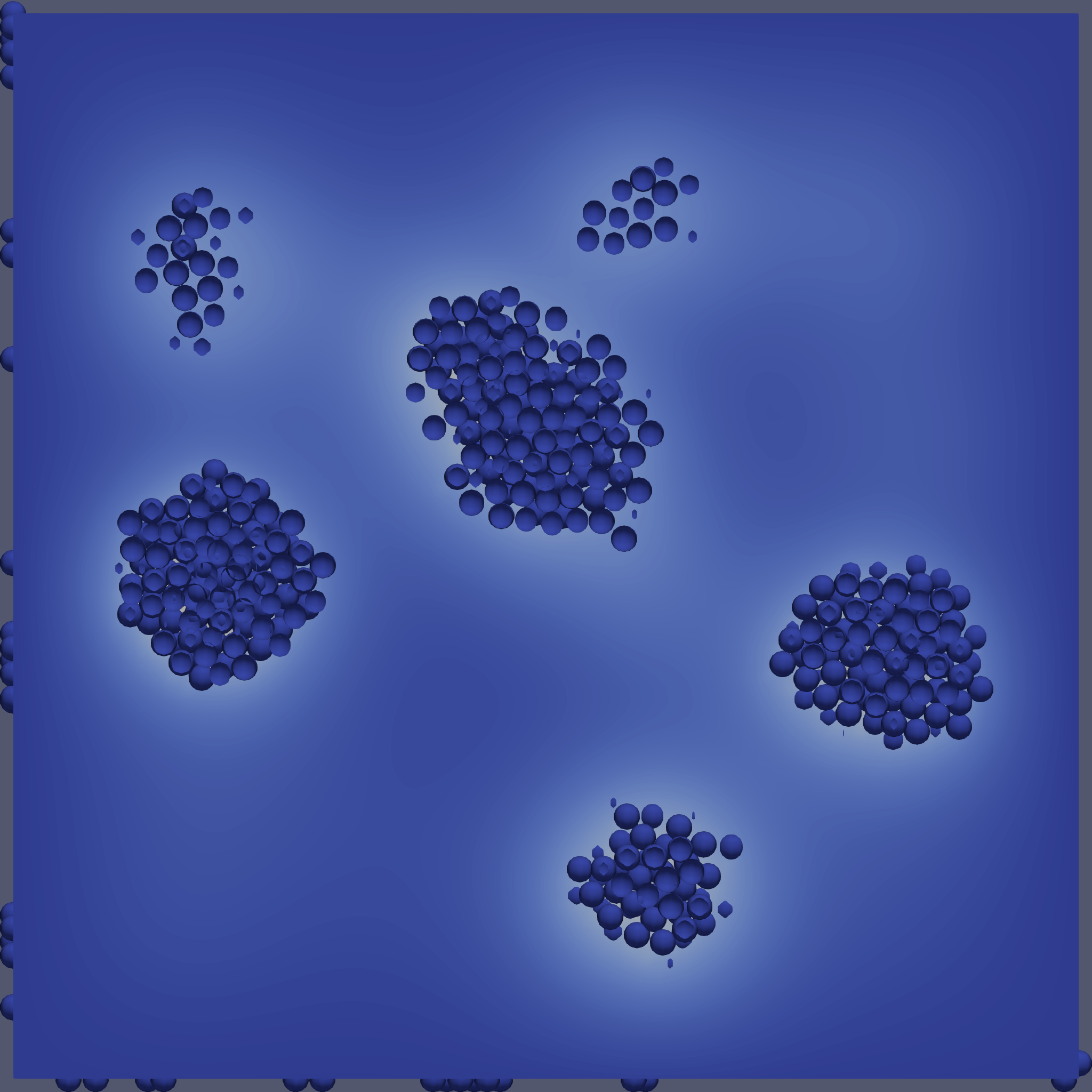
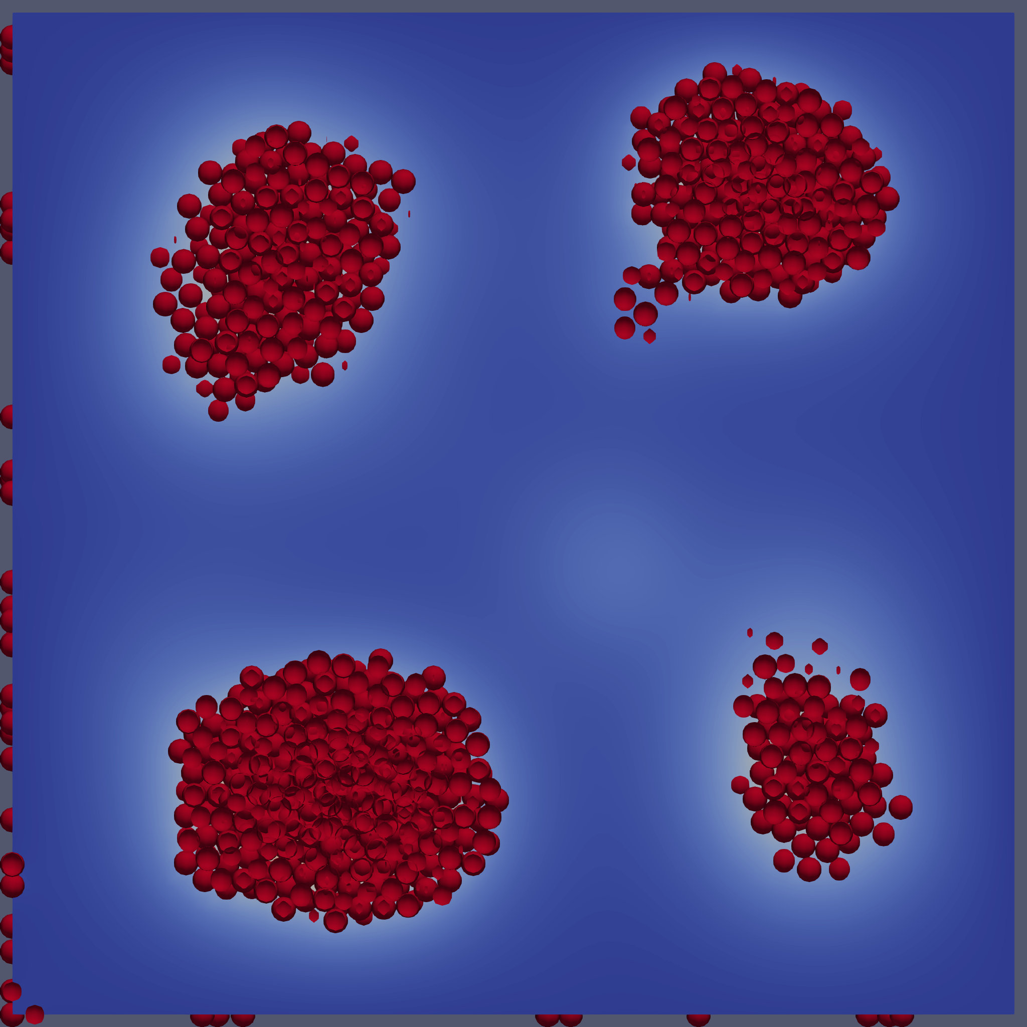
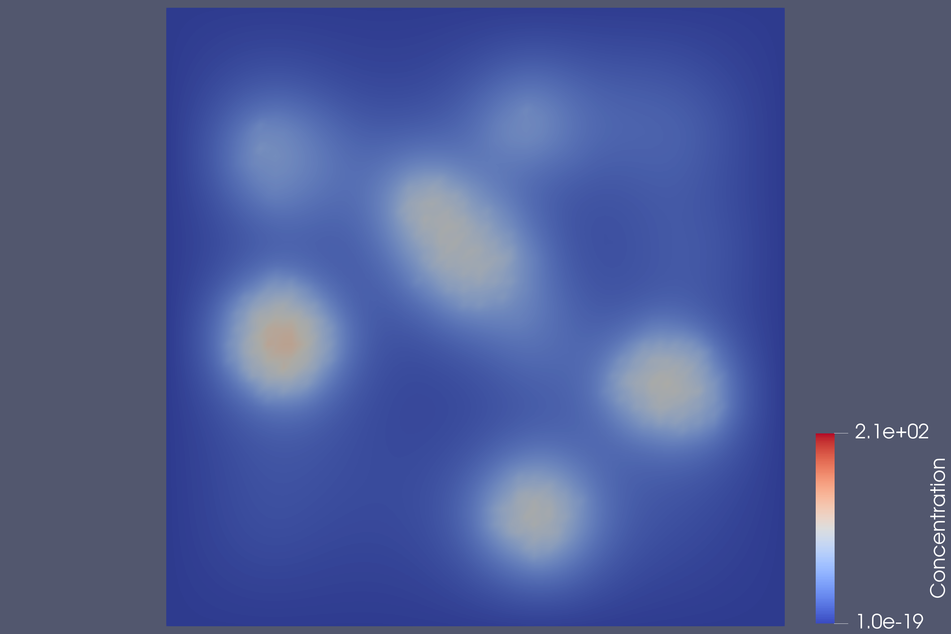
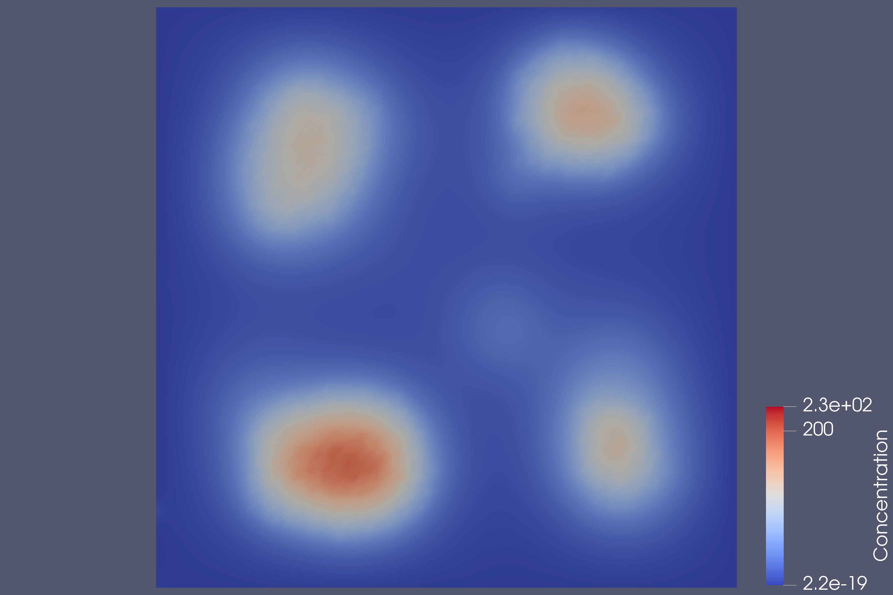
?figurename? 4.22: Soma clustering cross section. Cell positions coincide with regions of high substance concentration. The first row shows substance concentrations and cells, while the second row shows substance concentrations only. Columns show cell type with the corresponding substance.

Pyramidal Cell Growth Benchmark.

We used the pyramidal cell model from the neuroscience use case as a building block (see Figure 4.16). The simulation started with a 2D grid of initial neurons on the z-plane and started growing them. This simulation has three distinctive features. First, activity was limited to a neurite growth front, while the rest of the simulation remained static. This introduced a load imbalance for parallel execution. Second, the neurite implementation modified neighboring agents. Hence, synchronization was required between multiple threads to ensure correctness. Third, the simulation had only static substances, i.e., substance concentrations and gradients did not change over time.

4.7.2 Statistical Method

We perform five measurements for each presented data point in Figure 4.23 and Table 4.5. We summarize runtimes using the arithmetic mean and rates such as speedup using the harmonic mean.

4.7.3 Reproducibility

We use the latest BioDynaMo version v1.01-55-gd05111e3 for all use cases and benchmarks in this chapter. To help other researchers replicate our findings, we provide the following supplementary information for utmost transparency. First, we publish all source code and data in Supplementary File SF3 (SF3-code.tar.gz). The archive contains six shell scripts that execute all simulations, and generate all plots, visualizations and videos shown in this chapter. Second, we provide a ready-to-use self-contained Docker image to simplify the process of executing our simulations and benchmarks and to guarantee long-term reproducibility (SF4-bdm-publication-image.tar.gz). Third, we add a step-by-step instruction in SF2-reproduce-results.md.

4.7.4 Evaluation

First, to demonstrate the performance improvements against established ABS platforms, we compared BioDynaMo with Cortex3D and NetLogo. Figure 4.23A shows the speedup of BioDynaMo for four simulations. We define speedup as the runtime of the compared ABS platform over the runtime of BioDynaMo. We observed a significant speedup between 19 and 74$\times$ for Cortex3D and 25$\times$ for NetLogo. The speedup was larger when the simulation was more dynamic or more complex. Note that we set the number of threads available to BioDynaMo to one since Cortex3D and NetLogo are not parallelized. In the “epidemiology (medium-scale)” benchmark we increased the number of available physical CPU cores to 72 and observe a three order of magnitude speedup of 945$\times$. This result clearly shows the impact of parallelization on the overall performance. Although NetLogo is not parallelized, it benefits from parallel garbage collection. We could not perform a medium-scale analysis with Cortex3D, because it only supports simulations with a small number of agents.

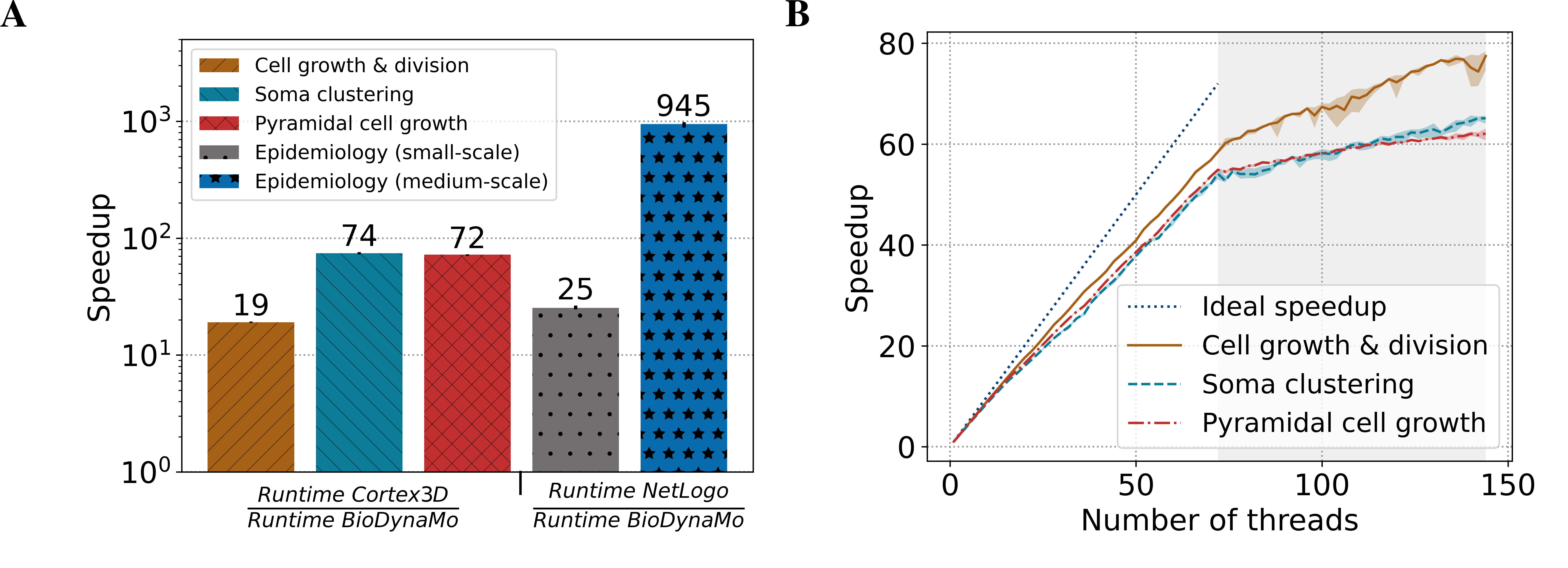
?figurename? 4.23: BioDynaMo performance analysis. (A) Speedup of BioDynaMo compared to the serial simulation platforms Cortex3D and NetLogo. Simulations use one CPU core except for the “epidemiology (medium-scale)” benchmark, for which all 72 physical cores were available. The comparison with NetLogo uses the same simulation with different numbers of agents. Cortex3D supports only small-scale simulations. (B) Strong scaling behavior of BioDynaMo on a server with 72 physical cores, two threads per core, and four NUMA domains. The grey area highlights hyper-threads.

Second, to evaluate the scalability of BioDynaMo, we measured the simulation time with an increasing number of threads. We increased the number of agents used in the comparison with Cortex3D and reduced the number of simulation timesteps to 10. Figure 4.23B shows the strong scaling analysis. We define the term “strong scaling” as the property of a simulation platform to reduce the runtime of a simulation with a fixed size $x$ with an increasing number of CPU cores $c$: $speedup(c,x)=\frac{time(1,x)}{time(c,x)}$ [410].

All simulation parameters were kept constant, and the number of threads was increased from one to the number of logical cores provided by the benchmark server. The maximum speedup ranged between 62$\times$ and 77$\times$, which corresponds to a parallel efficiency of 0.86 and 1.07. Performance improved even after all physical cores were utilized and hyper-threads were used. Hyper-threads are highlighted in gray in Figure 4.23B. We want to emphasize that even the pyramidal cell growth benchmark scaled well, despite the challenges of synchronization and load imbalance.

Third, we evaluated the impact of calculating the mechanical forces on the GPU using the cell growth and division, and soma clustering simulations. We excluded the pyramidal cell growth simulation because the current GPU kernel does not yet support cylinder geometry. The benchmarks were executed on System C (Table 4.4), comparing an NVidia Tesla V100 GPU with 32 CPU cores (64 threads). We observed a speedup of 1.01$\times$ for cell growth and division, and 4.16$\times$ for soma clustering. The speedup correlated with the number of collisions in the simulation. The computational intensity is directly linked with the number of collisions between agents.

In summary, in the scalability test, we observed a minimum speedup of 62$\times$. Furthermore, we measured a minimum speedup of 19$\times$ comparing BioDynaMo with Cortex3D both using a single thread. Based on these two observations, we conclude that on System A (Table 4.4) BioDynaMo is more than three orders of magnitude faster than Cortex3D. In the comparison with NetLogo we observed a 945$\times$ speedup directly.

Based on these speedups, we executed the neuroscience, oncology, and epidemiology use cases with one billion agents. Using all 72 physical CPUs on System B (Table 4.4), we measured a runtime of 1 hour 26 minutes, 6 hours 22 minutes, and 2 hours, respectively. One billion agents, however, are not the limit. The maximum depends on the available memory and accepted execution duration. To be consistent across all use cases and keep our pipeline’s total execution time better manageable, we decided to run these benchmarks with one billion agents. Table 4.5 shows that available memory would permit an epidemiological and neuroscience simulation with two billion agents. With enough memory, BioDynaMo is capable of supporting hundreds of billions of agents.

Simulation Agents Diffusion Iterations System Physical Runtime Memory volumes (Table 4.4) CPUs Neuroscience use case      Single (Figure 4.16A) 1 494 250 500 A 1 0.16 s 382 MB D 1 0.12 s 479 MB      Large-scale (Figure 4.16C) 9 036 986 65 536 500 A 72 35 s 6.47 GB D 2 11 min 28 s 5.37 GB      Very-large-scale 1 018 644 154 5 606 442 500 B 72 1 h 24 min 438 GB Oncology use case (Figure 4.19)      2000 initial cells 4 177 0 312 A 1 1.05 s 382 MB D 1 0.832 s 480 MB      4000 initial cells 5 341 0 312 A 1 1.76 s 382 MB D 1 1.34 s 480 MB      8000 initial cells 7 861 0 288 A 1 3.27 s 384 MB D 1 2.60 s 482 MB      Large-scale 1 000 3925 0 288 A 72 1 min 42 s 7.42 GB D 2 43 min 56 s 5.84 GB      Very-large-scale 986 054 868 0 288 B 72 6 h 21 min 604 GB Epidemiology use case (Figure 4.20C)      Measles 2 010 0 1000 A 1 0.53 s 381 MB D 1 0.42 s 479 MB      Seasonal Influenza 20 200 0 2500 A 1 16.41 s 383 MB D 1 16.40 s 479 GB      Medium-scale (measles) 100 500 0 1000 A 72 1.36 s 1 GB      Large-scale (measles) 10 050 000 0 1000 A 72 59.19 s 5.87 GB D 2 19 min 18 s 5.41 GB      Very-large-scale (measles) 1 005 000 000 0 1000 B 72 2 h 0 min 495 GB Soma clustering (Figure 4.21) 32 000 1 240 000 6 000 A 72 12.91 s 1.02 GB D 2 2 min 7 s 522 MB

?tablename? 4.5: Performance data. The values in column “Agents" and “Diffusion volumes" are taken from the end of the simulation. Runtime measures the wall-clock time to simulate the number of iterations. It excludes the time for simulation setup and visualization. The entries in column “System” correspond to Table 4.4.

4.8 Discussion

This chapter presented BioDynaMo, a novel open-source platform for agent-based simulations. Its modular software architecture allows researchers to implement models of distinctly different fields, of which neuroscience, oncology, and epidemiology were demonstrated in this chapter. Although the implemented models follow a simplistic set of rules, the results that emerge from the simulations are prominent and highlight BioDynaMo’s capabilities. We do not claim that these models are novel, but we rather want to emphasize that BioDynaMo enables scientists to (i) develop models in various computational biology fields in a modular fashion, (ii) obtain results rapidly with the parallelized execution engine, (iii) scale up the model to billions of agents on a single server, and (iv) produce results that are in agreement with validated experimental data. Although BioDynaMo is modular, we currently offer a limited number of ready-to-use simulation primitives. We are currently expanding our library of agents and behaviors to facilitate model development beyond the current capacity.

Ongoing work uses BioDynaMo to gain insights into retinal development [9], cryopreservation [183, 184], multiscale (organ-to-cell) cancer modelling [8, 10], radiation-induced tissue damage [23, 11, 25, 24], and more [41, 87, 18, 17]. Further efforts focus on accelerating drug development by replacing in vitro experiments with in silico simulations using BioDynaMo.

Our performance analysis showed improvements of up to three orders of magnitude over state-of-the-art baseline simulation software, allowing us to scale up simulations to an unprecedented number of agents. To the best of our knowledge, BioDynaMo is the first scalable ABS platform of neural development that scales to more than one billion agents. The same principles used to model axons and dendrites in the neuroscience use case could also be applied to simulate blood and lymphatic vessels.

We envision BioDynaMo to become a valuable tool in computational biology, fostering faster and easier simulation of complex and large-scale systems, interdisciplinary collaboration, and scientific reproducibility.

4.9 Availability and Future Directions

BioDynaMo is an open-source project under the Apache 2.0 license and can be found on Github (https://github.com/BioDynaMo/biodynamo). The documentation is split into three parts: API reference, user guide, and developer guide. Furthermore, a Slack channel is available for requesting assistance or guidance from the BioDynaMo development team.

BioDynaMo officially supports the following operating systems: Ubuntu (18.04, 20.04), CentOS 7, and macOS (10.15, 11.1). We test BioDynaMo on these systems and provide prebuilt binaries for third party dependencies: ROOT and ParaView.

All of the results presented in the chapter can be reproduced following the instructions in the Supplementary Information.

By designing BioDynaMo in a modular and extensible way, we laid the foundation to create new functionalities easily. We encourage the life science community to contribute their developments back to the open-source codebase of BioDynaMo. Over time, the accumulation of all these contributions will form the BioDynaMo open-model library, as shown in Figure 4.24. This library will help scientists accelerate their research by providing the required building blocks (agents, biological behavior, etc.) for their simulation. Currently, we collect these contributions in our Github repository (https://github.com/BioDynaMo/biodynamo).

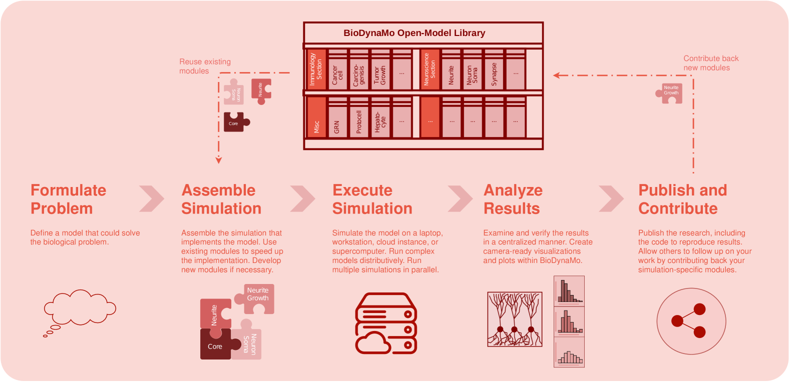
?figurename? 4.24: BioDynaMo platform. Vision of BioDynaMo, a platform to accelerate in silico experiments.

4.10 Supporting Information

All supporting information is available at: https://doi.org/10.5281/zenodo.3862368

SF2-reproduce-results.md

Instructions on how to reproduce all results presented in this chapter.

SF3-code.tar.gz

Codebase to reproduce all results presented in this chapter. This file contains all code necessary to reproduce performance results, plots, visualizations, and videos shown in this chapter. Furthermore, it contains more details about the hardware and software configuration of the different systems described in Table 4.4.

SF4-bdm-publication-image.tar.gz

Docker image to reproduce all results presented in this chapter. We provide a Docker image to simplify the process of executing our simulations and benchmarks and to guarantee long-term reproducibility. The only requirement that users must install is a recent version of the Docker engine. All other prerequisites are already provided in the ready-to-use, self-contained Docker image. This approach does not rely on content hosted somewhere on the internet that might become unavailable in the future.

SF5-raw-results.tar.gz

Raw results. This archive contains all raw results from the simulations and benchmarks shown in this chapter.

SV1-single-pyramidal-cell.mp4

Single pyramidal cell growth simulation, as shown in Figure 4.16A.

SV2-large-scale-neuronal-development.mp4

Large-scale pyramidal cell growth simulation, as shown in Figure 4.16C.

SV3-tumor-spheroid.mp4

Tumor spheroid growth simulation, as shown in Figure 4.19B.

SV4-soma-clustering.mp4.

Soma clustering simulation, as shown in Figure 4.21.

?chaptername? 5 BioDynaMo’s Simulation Engine

5.1 Introduction

Agent-based modeling (ABM) allows to simulate complex dynamics in a wide range of research fields. ABM has been used to answer research questions in biology [27, 187, 114], sociology [411], economics [412], technology [413], business [157], and more fields [414]. Agents are individual entities that, among others, can represent subcellular structures to simulate the growth of a neuron, a cell to investigate cancer development, or a person to simulate the spread of infectious diseases [188]. The actions of an agent are defined through instances of class behavior. To stay with the examples from before, possible behaviors are neurite bifurcation, uncontrolled cell division, or infection.

Agent-based models are developed in an iterative way, during which an initial model is increasingly refined until it matches with observed data [214, 306]. Model parameters that cannot be derived from the literature are determined through optimization. An optimization algorithm generates a parameter set, executes the model, and evaluates the error with respect to observed data until the error converges to a local or global minimum. This loop might also contain an uncertainty analysis to evaluate the robustness of a solution [415]. Consequently, the model must be simulated many times.

The simulation engine’s performance limits the scale of the model and determines how often the model can be simulated. Thus, performance is a key issue for simulating models on extreme scales that might one day be able to simulate all 86 billion neurons in the brain [391]. It is also crucial for smaller-scale simulations to explore vast parameter space, analyze parameter uncertainty, repeat the simulation often enough to reach statistical significance, and develop models rapidly.

To achieve these goals, we present a novel simulation engine called BioDynaMo, which is optimized for high performance and scalability. During its development, we identify the following three main performance challenges for agent-based simulations.

Challenge 1: To fully utilize systems with high processor core counts, the parallel part of the simulation engine has to be maximized (see Amdahl’s law [416]). Although it is easy to parallelize the loop over all agents (Algorithm 8), our benchmarks revealed two operations whose level of parallelization has a significant performance impact. First, building the environment index, which is used to determine the neighbors of an agent. The literature describes various radial-neighbor search algorithms with different design trade offs between build and search performance. Second, combining thread-local results at the end of each iteration. In general, attention must also be paid to seemingly minor things, such as resizing a large vector, which by default is initialized by a single thread.

Challenge 2: ABMs are predominantly memory-bound due to two reasons. First, the behavior of agents often has low arithmetic intensity. Second, ABM can be very dynamic. During a simulation, agents move through space, change their behavior, and are created and destroyed. Consequently, the neighborhood of an agent changes continuously, leading to an irregular memory access pattern and poor cache utilization. This results in large data movement between the main memory and the processor cores.

Challenge 3: Under certain conditions, the expensive calculation of mechanical forces between agents is redundant (Section 5.5). These forces are for example used in tissue models to determine the displacement of agents. The challenge is identifying those agents for which the pairwise force calculation can be safely omitted.

BioDynaMo addresses these challenges with the following new optimizations. To maximize the parallelization (Challenge 1), we develop an optimized uniform grid to search for agent neighbors and fully parallelize the addition and removal of agents. We address the data movement bottleneck (Challenge 2) in software by (i) optimizing the iteration over all agents on systems with non-uniform memory architecture, (ii) sorting agents and their neighbors to improve the cache hit rate and minimize access to remote DRAM, and (iii) introducing a pool memory allocator. To avoid redundant mechanical force calculations (Challenge 3), we add a mechanism to detect agents for which we can guarantee that the resulting force will not move the agent.

These mechanisms make BioDynaMo nearly an order of magnitude more efficient than Biocellion and three orders of magnitude faster than Cortex3D and NetLogo. The performance improvements account for a median speedup of 159$\times$ compared to BioDynaMo’s standard implementation with all optimizations turned off. As a result, BioDynaMo is able to simulate 1.72 billion agents on one server. The main contributions of this chapter are as follows.

• We present a novel high-performance agent-based simulation engine. The engine can be used in many domains due to its modular software design and features a specialization for neuroscience, capable of simulating the development of neurons.

• We present six optimizations to maximize performance (Section 5.3–5.5). These insights are transferable and can be used to improve the performance of other agent-based simulators.

• We present an in-depth evaluation of BioDynaMo’s performance using five different simulations (Section 5.6). This comprehensive analysis provides insights for users of BioDynaMo into which parameters yield the best performance and hints for developers of future agent-based simulation tools.

5.2 BioDynaMo’s Simulation Engine

This section gives an overview of BioDynaMo and its components. BioDynaMo is written in C++, uses OpenMP [417] for shared-memory parallelism, and is available under the Apache 2.0 open-source license.

Breitwieser et al. [188] describe the user-facing features of the BioDynaMo platform and detail its modular software design and ease-of-use by means of three use cases in the domains of neuroscience, epidemiology, and oncology.

BioDynaMo is a hybrid framework able to utilize multi-core CPUs and GPUs. This dissertation focuses on the CPU version, which has two major advantages. First, the CPU version can simulate many more agents than a GPU version. The reason is that GPUs have typically significantly smaller memory than CPUs. For example, our benchmark hardware has 12$\times$ more memory than the current flagship GPU from NVidia, the A100 [418]. Second, the CPU version improves the usability and flexibility for our broad user community, who often only have a Matlab [419] or R [420] coding background. In BioDynaMo, users create simulations by writing C++ code. A GPU-only version would require users to write CUDA code to define new agents, behaviors, and other user-defined components. Therefore, BioDynaMo only offloads computations to the GPU, transparently to the user [421].

The main objects in agent-based simulations are agents, behaviors, and operations. Agents (e.g., a cancer cell) have attributes that are updated through behaviors and operations. Behaviors (e.g., uncontrolled cell division) are functions that can be assigned and removed from an agent and give users fine-grained control over the actions of an agent. In contrast, Agent operations are executed for each agent. For example, to calculate the mechanical forces between agents and execute all individual behaviors of an agent. The second type of operation, called standalone operation is executed once per iteration to perform a specific task (e.g., visualization). A characteristic property of agent-based simulation is local interaction. BioDynaMo provides a common interface for different neighbor search algorithms called environment. Besides the uniform grid detailed in Section 5.3.1, BioDynaMo features a kd-tree based on nanoflann [422] and octree based on the publication of Behley et al. [339].

The agent-based simulation algorithm (Algorithm 8) comprises two steps. First, users have to define the starting condition of the model (L1) in which agents, behaviors, operations, and any other resource are created. Second, the simulation engine executes this model for a number of iterations (L2–19). The engine executes all agent operations for each agent (L7–12) and all standalone operations (L12–14). Standalone operations can be further separated into operations that must be executed at the beginning of the iteration (e.g., to update the environment index [L3-5]) or the end (e.g., visualization [L16-18]). There are two barriers synchronizing threads (L6 and L15).

1

2

3ModelInitialization()

4for $i\in iterations$ do

5    for $op\in pre\_standalone\_operations$ do

6       $op()$;

7      

8    end for

9   

10   wait()

11   parallel for $a\in agents$ do

12       for $op\in agent\_operations$ do

13          $op(a)$;

14         

15       end for

16      

17    end

18   for $op\in standalone\_operations$ do

19       $op()$;

20      

21    end for

22   

23   wait()

24   for $op\in post\_standalone\_operations$ do

25       $op()$;

26      

27    end for

28   

29 end for

30

Algorithm 8 Simulation algorithm

5.2.1 Alternative Execution Modes

BioDynaMo offers different execution modes that influence how simulations are executed to cater to different user needs. These execution modes can also be combined.

Row-Wise vs. Column-Wise Execution Mode.

For each iteration, the execution engine has to execute a set of operations for each agent (Algorithm 8 L7–12). We can look at this as a matrix with one column per agent and one row per operation. Each element in the matrix—corresponding to an agent-operation pair—must be executed. Execution can happen in column-wise order, in which all operations are executed for one agent before proceeding to the following agent, or in a row-wise order in which one operation is executed for each agent before proceeding to the next operation. Algorithm 8 shows the default column-wise order, which can be transformed to the row-wise order by exchanging lines seven and eight.

RandomizedRm.

The ResourceManager, an essential class in the simulation engine, stores raw agent pointers and offers functions to add, remove, get, and iterate over agents. The RandomizedRm class is a decorator for ResourceManager and possible subclasses and randomizes the iteration order over all agents after each iteration. This feature is important to avoid an execution order bias for specific models [197].

Different Execution Contexts.

The execution context is a facade for the environment interface and the resource manager. There is one instance of this object per thread. This class aims to encapsulate discretization choices: When should changes to an agent be visible to other agents? When should new or removed agents be visible? Currently, BioDynaMo provides the in-place and copy execution context. If the user chooses the in-place execution context, changes to an agent are immediately visible to its neighbors. Consequently, neighbor attributes might already be updated to the current iteration if the neighbor has been processed before. Thus the neighbor attributes do not contain the values of the previous iteration anymore. In contrast, the copy execution context updates agent copies and commits the changes at the end of the iteration after all agents have been updated. For both execution context types, agent removals and additions take effect at the beginning of the next iteration. Users can provide additional execution contexts in which different discretization choices are made.

5.3 Maximize Parallelization

5.3.1 Grid-Based Neighbor Search

Determining the neighbors of an agent is a pre-condition for all agent interactions. For example, the infection behavior in an epidemiological model requires information if any of the immediate neighbors is infected. In this context, it is essential to find neighbors fast and efficiently and minimize the build time of the required index. Building an index in every iteration has a high cost, as shown in the evaluation section. We exploit the fact that the interaction radius is known at the beginning of the iteration. For this fixed-radius search problem, a grid-based solution is a good choice because the box of an agent can be determined in constant time using the agent’s position [339]. This is confirmed by our evaluation in Section 5.6.9. The build stage in which all agents are assigned to a box can be easily parallelized. In the search stage, the grid determines all neighbors by iterating over all agents in the same box and the surrounding boxes. In 3D space, we consider the 3x3x3 cube of boxes surrounding and including the query box. All agents inside a box are stored in an array-based linked list. The box only needs to store the start index and the number of elements it contains. To avoid zeroing all boxes at the beginning of the build stage, we add a timestamp attribute to each box, updated whenever an agent is added. Consequently, we can determine that a box is empty if the simulation and box timestamp is different. Therefore, we can build the grid in $O(\#agents)$ time instead of $O(\#agents+\#boxes)$, which is relevant for large simulation spaces that are not fully populated.

The array-based linked list uses the same agent indices as in the ResourceManager. The ResourceManager, an essential class in the simulation engine, stores raw agent pointers and offers functions to add, remove, get, and iterate over agents. Thus, it also benefits from the memory layout optimization presented in Section 5.4.2. This optimization reduces the distance in memory of agents that are close in space. Consequently, linked list elements will be closer to each other, improving the cache hit rate of traversing the linked list during the search stage of the grid. The described grid implementation can be found in the class UniformGridEnvironment.

5.3.2 Adding and Removing Agents in Parallel

To maximize the theoretically achievable speedup described in Amdahl’s law [416], we maximize the parallel part of the simulation by parallelizing the addition and removal of agents. By default, BioDynaMo stores a thread-local copy of additions and removals and commits them to the ResourceManager at the end of each iteration.

Additions are trivial; the engine determines the total number of additions, grows the data structures in the ResourceManager, and adds the agent pointers in parallel. In contrast, the parallelization of removals is a more elaborate process because we disallow empty vector elements in the ResourceManager. If the simulation engine has to remove an agent stored in the middle of the vector, it must swap it with the last element before shrinking it. The following algorithm aims at performing the necessary swaps and updates in dependent data structures in parallel. Figure 5.1 illustrates the parallelized algorithm simplified for a single NUMA domain.

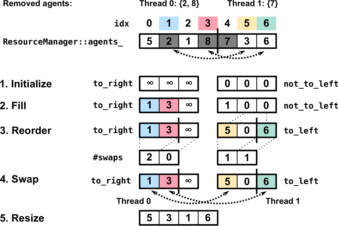
?figurename? 5.1: Parallel agent removal mechanism

This example assumes a simulation with seven agents represented with identifier 1–7 and two threads, which remove three agents from the simulation. These agents are highlighted with a grey background. The other colors serve as a visual aid to track the agents that must be swapped.

The algorithm comprises five main steps. First, the algorithm determines the total number of removed agents, calculates the new size of the vector ($old\_size-removed\_agents$), and initializes two auxiliary arrays. The size of the auxiliary arrays equals the number of removed agents. The new vector size is indicated by the vertical line between indexes three and four in Figure 5.1.

Second, each thread iterates over its vector of removed agents and fills the auxiliary arrays. If the agent is stored to the left of the new size index, it must be moved to the right. Therefore the algorithm inserts the element index into the array $to\_right$. If the agent is stored to the right of the new size, we insert a one into array $not\_to\_left$ at the index: $idx-new\_size$. The maximum index used to access elements in the auxiliary array is smaller than the number of removed agents and is independent of the number of remaining agents.

Third, we partition the two auxiliary arrays into blocks corresponding to the total number of threads. A thread iterates over its auxiliary block, moves entries to the beginning if they indicate a swap, and stores a counter in the #swaps array. For the $to\_right$ array, the algorithm skips or overwrites elements with the value $UINT\_MAX$. In this step, the semantic of the $not\_to\_left$ array changes to $to\_left$. Thus, the algorithm looks for all zeros in the array, replaces them with the value $array\_index+new\_size$, and moves them to the beginning of the block.

In the fourth step, we can finally perform the swaps. The algorithm calculates the prefix sum of the two $\#swaps$ arrays and partitions the swaps among all threads. Each thread can determine the indices based on the prefix sum of $\#swaps$.

In the last step, the algorithm completes the removal by shrinking the vector to $new\_size$.

This algorithm requires $O(removed\_agents)$ time and space and parallelizes steps 1–4.

5.3.3 Visualization

Visualization plays an essential role in gaining insights into the dynamics of a simulation during its iterative development process. ParaView [392] is a feature-rich and powerful visualization package that uses MPI to parallelize work on multiple processes, but its shared-memory parallelism is severely limited. In contrast, BioDynaMo only uses one process and is parallelized with OpenMP. Therefore, the integration of ParaView and BioDynaMo performs poorly. To resolve this performance bottleneck, we present a solution where BioDynaMo exports visualization files using shared-memory parallelism first, which ParaView renders in a second step using multiple processes.

To that extent, we present three optimizations to minimize the visualization time. First, we parallelize ParaView’s (p)vtu and (p)vti data writer using OpenMP. Although ParaView provides a parallelized implementation using MPI, this solution is not amenable for shared-memory applications, as mentioned before. Second, we introduce on-demand export of agent attributes based on just-in-time (JIT) compilation with cling [423]. Instead of exporting all agent attributes, we divide them into obligatory and optional ones. Obligatory attributes are defined in the agent implementation, are essential to render its geometry (e.g., position and diameter of a sphere), and are therefore exported by default. The user must explicitly request all other agent attributes by setting a parameter in a configuration file, command-line argument, or directly in the code. Third, we introduce an interface that gives third-party software like ParaView rapid access to agent attributes.

Figure 5.2 illustrates how ParaView’s request for the diameter of cell with ID 5 is handled. BioDynaMo instantiates a MappedDataArray for each selected attribute of each agent type, which receives data requests from ParaView’s file writer. This request is forwarded to the type index, which holds a vector of agent pointers that belong to a specific class . ParaView’s request ID indexes the vector . The vector element points to the beginning of the agent object on the heap . We add the attribute offset to the base class pointer and return the data to the MappedDataArray . The attribute offset is determined during the build process in which we use ROOT [361] to collect reflection information for all relevant classes. The MappedDataArray supports three execution modes: zero-copy, cache, and copy. In the zero-copy mode, the data element is returned to ParaView directly . In the cache and copy mode, each MappedDataArray instance instantiates a data vector. In cache mode, this data vector is filled on-demand in step . All consecutive requests to the same ID will be serviced from the internal data vector, bypassing steps – . In the copy mode, the internal data vector is completely filled before any requests can be made. Similar to the cache hit scenario, all requests will be served directly from the internal data vector. The described mechanism could also be used to integrate other third-party software packages into BioDynaMo.

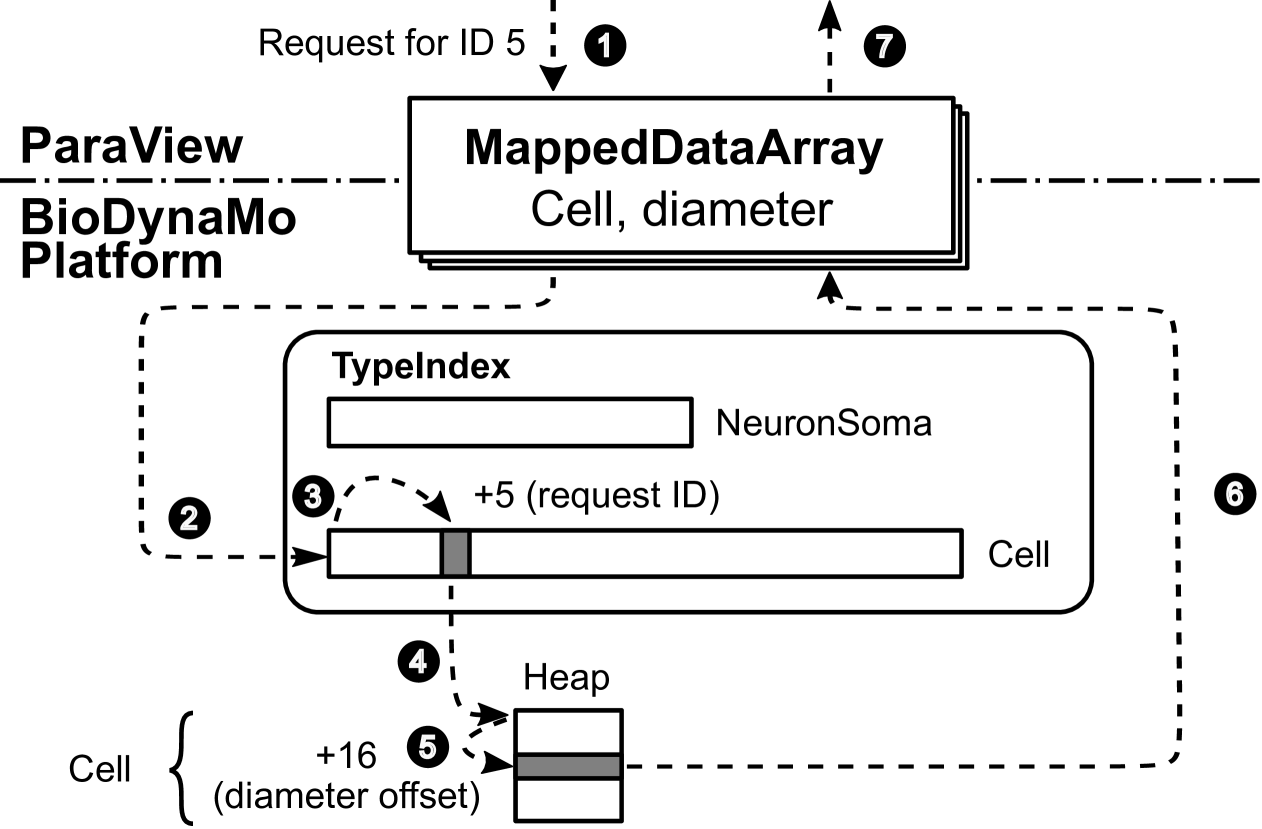
?figurename? 5.2: Interface between BioDynaMo and ParaView

5.4 Optimize Memory Layout and Data Access Pattern

5.4.1 NUMA-Aware Iteration

BioDynaMo supports systems with multiple NUMA domains. We add a mechanism to match threads with agents from the same NUMA domain to minimize the traffic to remote DRAM because OpenMP does not provide this functionality.

Figure 5.3 shows a server with two NUMA domains (ND0, ND1) corresponding to two CPUs with two threads each (T0 & T1, T2 & T3).

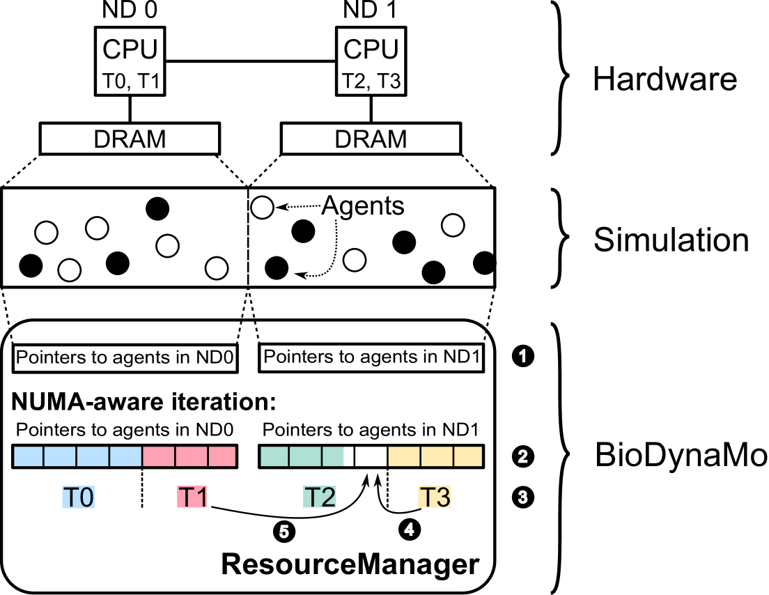
?figurename? 5.3: NUMA-aware iteration

The CPUs have a local DRAM with shorter memory access latency than the remote DRAM. The agents in the simulation are balanced between the two NUMA domains (see Section 5.4.2). The ResourceManager maintains a vector of agent pointers for each NUMA domain . To iterate over agents in a NUMA-aware way, BioDynaMo first partitions these vectors into blocks of agent pointers of the same size . Second, these blocks are partitioned among the threads from the matching NUMA domain . Threads process the assigned blocks in parallel. Figure 5.3 shows processed blocks with a background color of the corresponding thread.

We implement a two-level work-stealing mechanism to avoid imbalanced execution times across threads. First, a thread can steal a block from a different thread from the same NUMA domain (e.g., ). Second, if the thread’s NUMA domain has already finished all work, the thread can steal work from a different NUMA domain (e.g., ).

5.4.2 Agent Sorting and Balancing

To accelerate the memory-bound simulations, we must increase the cache hit ratio and load balance the agents among NUMA domains to minimize remote DRAM accesses. In Section 5.4.1 and Figure 5.3, we assume this is already the case. This section presents an efficient algorithm to achieve this goal by sorting the agents’ memory locations and preserving the neighborhood relations in 3D. Preserving the neighborhood relation and reducing the dimensionality is the main characteristic of space-filling curves (e.g., Morton order [336] or Hilbert curve [337]).

We compared the performance of the Morton order with the Hilbert curve using an oncological simulation [188] and observed a negligible performance improvement of 0.54% from using the Hilbert curve. Higher costs to decode the Hilbert curve offset small gains for the agent operations. Therefore, we use the Morton order because it results in simpler code.

Figure 5.4 and the following description present the algorithm in 2D space, but the same principles apply in 3D. In BioDynaMo, the neighborhood information is stored in the implementation of the environment interface.

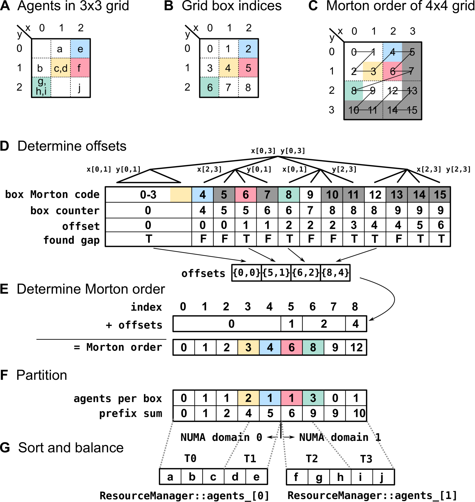
?figurename? 5.4: Agent sorting and balancing mechanism

Since the uniform grid environment performs best, as shown in the evaluation section (Section 5.6.9), we utilize its characteristics to achieve fast sorting and balancing. We assume the following scenario. Agents are stored in a 3$\times$3 uniform grid (A). The simulation runs on a system with two NUMA domains and two threads per domain, resulting in four threads. The grid boxes are stored in a flattened array. Figure 5.4B shows the box indices for x and y coordinates. We apply a Morton order space-filling curve [336] on the uniform grid (C). Our goal is to sort the agents in the nine boxes in increasing Morton order. The Morton order is only contiguous for quadratic simulation spaces where the length is a power of two. Therefore, C shows a 4$\times$4 grid. For the 3$\times$3 simulation space, there are gaps between Morton code four and six, six and eight, and nine and twelve.

The algorithm comprises three main steps. First, the algorithm determines the sequence of boxes in Morton order (D, E). Second, the algorithm partitions the boxes into segments that balance agents among NUMA domains and threads (F). Third, the algorithm stores the agents in their new position in the resource manager (G). In Figure 5.4, we selected four boxes and colored them in red, green, blue, and yellow to quickly find the corresponding entries for contained agents, box index, and Morton code. The boxes outside the simulation space have a grey background.

In the first main step (D, E), we determine all gaps between grid boxes in simulation space (D) to avoid a costly sorting operation or iteration over all $N\times N$ boxes, where $N$ is the next higher power of two of $max(x,y)$. We exploit the fact that the Morton order corresponds to a depth-first traversal of a quadtree, in which each box is a leaf in the tree. Leaves whose boxes are outside the simulation space are considered empty. Similarly, an inner node is empty if all of its corresponding leaves are outside the simulation space. If all the corresponding boxes of an inner node are inside the simulation space (i.e., the inner node has a perfect subtree), we say the inner node is complete. The quadtree is only an abstraction and does not need to be constructed. It is only necessary to store the current traversal path, which requires $O(log(\#boxes))$ space.

The mechanism in D uses three auxiliary variables: box counter, offsets, and found_gap, which are initialized to zero, zero, and true. The matrix in Figure 5.4D shows the three variables before the update of the current traversal step. The algorithm traverses the tree depth-first and continues to the next deeper tree level only if the current node is neither complete nor empty. In this case, the variables are not changed. If a complete inner node or leave inside the simulation space is found and the found_gap variable is true, the algorithm adds an entry with the current box counter and offset values in the offsets array and clears found_gap. Afterward, the box counter variable is incremented by the number of leaves in its subtree or one if it was a leave, irrespectively of the former value of found_gap. Empty nodes or leaves are handled similarly. The offset variable is incremented by the number of empty leaves in the subtree of an empty node or one if it is an empty leave. Additionally, the found_gap variable is set to true. The algorithm keeps track of the x and y intervals to calculate (in constant time) the number of leaves in a subtree and determine if an inner node is entirely, partially, or not inside the simulation space.

With the already sorted offsets array, the Morton order can be determined in linear time by iterating over all indices and adding the corresponding offset (E).

In the second main step (F), the algorithm iterates over all boxes in Morton order and fills an auxiliary array with the number of agents in each box. Afterward, the algorithm calculates the prefix sum of the auxiliary array in a parallel work-efficient manner [424] and partitions the total number of agents in the simulation such that each NUMA domain receives a share corresponding to its number of threads. Inside a NUMA domain, the agents are further partitioned such that each thread in this domain receives an equal share.

In the third main step (G), the threads copy the agents and store the pointer in the new position in the resource manager. The simulation engine can immediately free obsolete agents’ memory or delete all old copies after the step is finished. The latter requires more memory but might improve performance due to a more optimal memory layout in conjunction with the BioDynaMo memory allocator (Section 5.4.3).

The presented algorithm runs in $O(\#agents+\#boxes)$ time and space and parallelizes steps E–G.

5.4.3 BioDynaMo Memory Allocator

To improve the performance of the simulation engine, we present a custom dynamic memory allocator which improves the memory layout of the most frequently allocated objects in a simulation: agents and behaviors. Our solution builds upon pool allocators due to their constant time allocation performance. Pool allocators divide a memory block into equal-sized elements and store pointers to free elements in a linked list.

We create multiple instances of these allocators because they can only return memory elements of one size. As a result, agents and behaviors with distinct sizes are separated and stored in a columnar way. We separate the pool allocator into multiple NUMA domains (class NumaPoolAllocator) to fully control where memory is allocated. The NumaPoolAllocator has a central free-list and thread-private ones to minimize synchronization between threads. List nodes, which correspond to free memory locations, can be migrated between thread private and the central list, which is essential to avoid memory leaks. Migrations are triggered if a thread-private list exceeds a specific memory threshold. Lists minimize these migrations, and thus thread synchronization, by maintaining additional skip lists. These skip lists support additions and removals of a large number of elements in constant time.

Memory is allocated in large blocks with exponentially increasing sizes controlled by the parameter mem_mgr_growth_rate. The initialization of these memory blocks, which includes list node generation, is performed on-demand in smaller segments to minimize the required worst-case allocation time.

Every allocated memory block is divided into N-page aligned segments (Figure 5.5A), where N can be set with parameter mem_mgr_aligned_pages_shift.

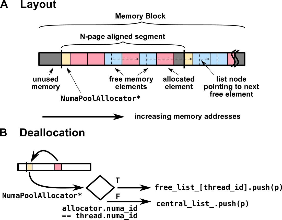
?figurename? 5.5: BioDynaMo’s memory allocator

The linked list nodes are stored inside free memory elements and do not require extra space. At the beginning of each N-aligned segment, we write the pointer to the corresponding NumaPoolAllocator instance. Therefore, allocated memory elements can obtain this pointer in constant time, based on their memory address. This solution enables constant time deallocations (see Figure 5.5b) but wastes memory in three ways. First, memory blocks are allocated using numa_alloc_onnode (libnuma [425]). This function does not return N-page aligned pointers and causes unusable regions at the beginning and the end, which sum up to $N*page\_size$ bytes. Second, there might not be enough space to place a whole element at the end of an N-page aligned segment. Elements must not cross N-page aligned borders because it would overwrite the necessary metadata. Third, the metadata requires the size of a pointer, which is eight bytes on 64-bit hardware. The amount of wasted memory is bounded by the following equation: $N*page\_size+element\_size+metadata\_size$. Despite this memory overhead, our performance evaluation shows that the BioDynaMo pool allocator uses on average less memory than ptmalloc2 and jemalloc [426]. Another side effect of this design choice is that the allocation size is limited by $N*page\_size-metadata\_size$.

5.5 Omit Collision Force Calculation

The most time-consuming operation in the tissue models presented in Section 5.6.1 is the calculation of the displacement of agents based on all mechanical forces. For this purpose, the simulation engine has to calculate pairwise collision forces between agents and their neighbors implemented in the class InteractionForce. By default, BioDynaMo uses the force calculation method detailed in the Cortex3D paper [39]. We observe that simulations can contain a significant amount of regions where agents do not move. Neural development simulations (see Section 5.6.1), for example, might only have an active growth front, while the remaining part of the neuron is unchanged.

Therefore, we present a mechanism to detect agents for which it is safe to skip the expensive force calculation. We call these agents static.

The following four conditions must be fulfilled in the last iteration: (i) the agent and none of its neighbors moved (ii) the agent’s and neighbors’ attributes did not change in a way that could increase the pairwise force (e.g., larger diameter), or the resulting displacement, (iii) new agents were not added within the interaction radius of the agent, and (iv) there is maximum one neighbor force which is non-zero.

The detection mechanism is closely tied to the InteractionForce implementation (see [188]), as condition two implies, and might have to be adjusted if a different force implementation is used.

Condition four is needed because we want to allow agents to shrink and to be removed from the simulation without setting the agents in this region to not static. Consequently, we have to ensure that two or more neighbor forces did not cancel each other out in the previous iteration.

The simulation engine monitors if any of the conditions are violated for each agent and sets the affected agents to not static. In this process, a distinction has to be made whether the changed attribute affects only the current agent or also its neighbors. If, for example, a static agent moves, the agent and all its neighbors will be affected, while a change to the agent’s force threshold, which must be exceeded to move the agent, only affects itself.

5.6 Evaluation

5.6.1 Benchmark Simulations

We use five simulations to evaluate the performance of the simulation engine: cell proliferation, cell clustering, and use cases in the domains of epidemiology, neuroscience, and oncology. These simulations use double-precision floating point variables and are described in detail in [188]. Table 5.1 shows that these simulations cover a broad spectrum of performance-related simulation characteristics and contain information about the number of agents, diffusion volumes, and iterations executed. We set the number of agents between two and 12.6 million to keep the total execution time of all benchmarks manageable. This is necessary due to the slow execution of the various baselines. In addition, Section 5.6.4 shows a benchmark in which each simulation is executed with one billion agents. Also the comparison with Biocellion in Section 5.6.5 contains a benchmark with 1.72 billion cells.

?tablename? 5.1: Performance-relevant simulation characteristics.

Characteristic	Cell proliferation	Cell clustering	Epidemiology	Neuroscience	Oncology
Create new agents during simulation	✗			✗	✗
Delete agents during simulation					✗
Agents modify neighbors				✗
Load imbalance			✗	✗
Agents move randomly			✗		✗
Simulation uses diffusion		✗		✗
Simulation has static regions				✗
Number of iterations	500	1000	1000	500	288
Number of agents (in millions)	12.6	2	10	9	10
Number of diffusion volumes	0	54m	0	65k	0

5.6.2 Experimental Setup and Reproducibility

All tests were executed in a Docker container with an Ubuntu 20.04 based image. Table 5.2 gives an overview of the main parameters of the three servers we used to evaluate the performance of BioDynaMo. If it is not explicitly mentioned, assume that System A was used to execute a benchmark.

We provide all code, the self-contained docker image, more detailed information on the hardware and software setup, and instructions to execute the benchmarks in the supplementary materials (https://doi.org/10.5281/zenodo.6463816).

?tablename? 5.2: Benchmark hardware

System	Memory	CPU	OS
A	504 GB	Four Intel(R) Xeon(R) E7-8890 v3 CPUs @ 2.50GHz with a total of 72 physical cores, two threads per core and four NUMA domains.	CentOS 7.9.2009
B	1008 GB
C	62 GB	Two Intel(R) Xeon(R) E5-2683 v3 CPUs @ 2.00GHz with a total of 28 physical cores, two threads per core and two NUMA domains.	CentOS Stream 8

5.6.3 General Performance Metrics

We characterize the agent-based simulation workload by breaking down the operation’s execution time, and exploring microarchitecture inefficiencies.

The following benchmarks were performed with all optimizations enabled. Figure 5.6 shows a breakdown of all operations in our benchmark simulations.

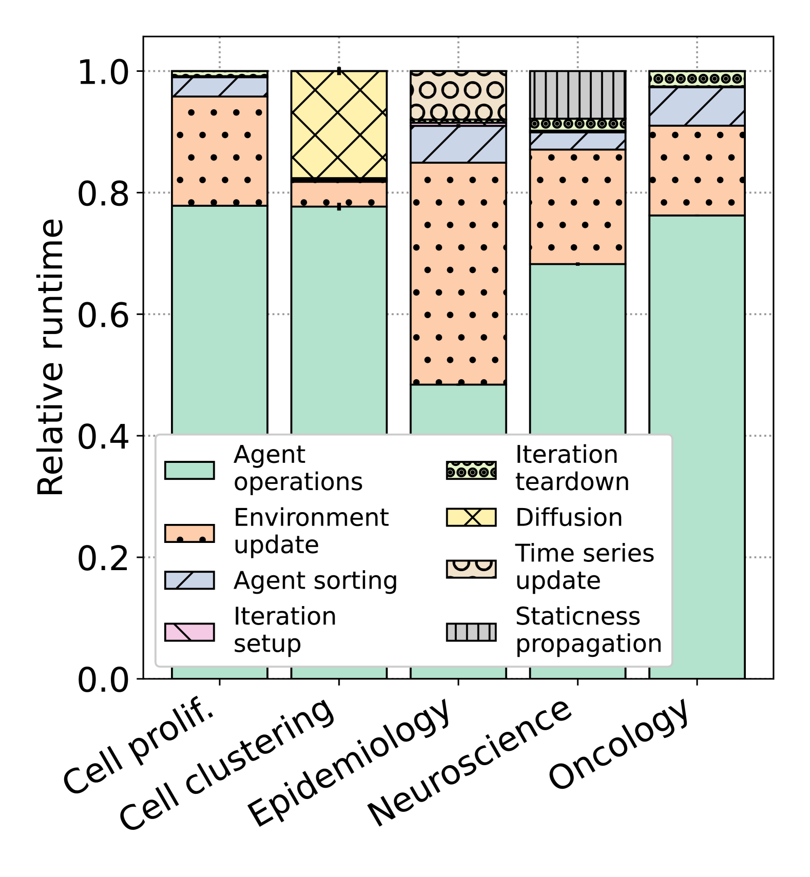
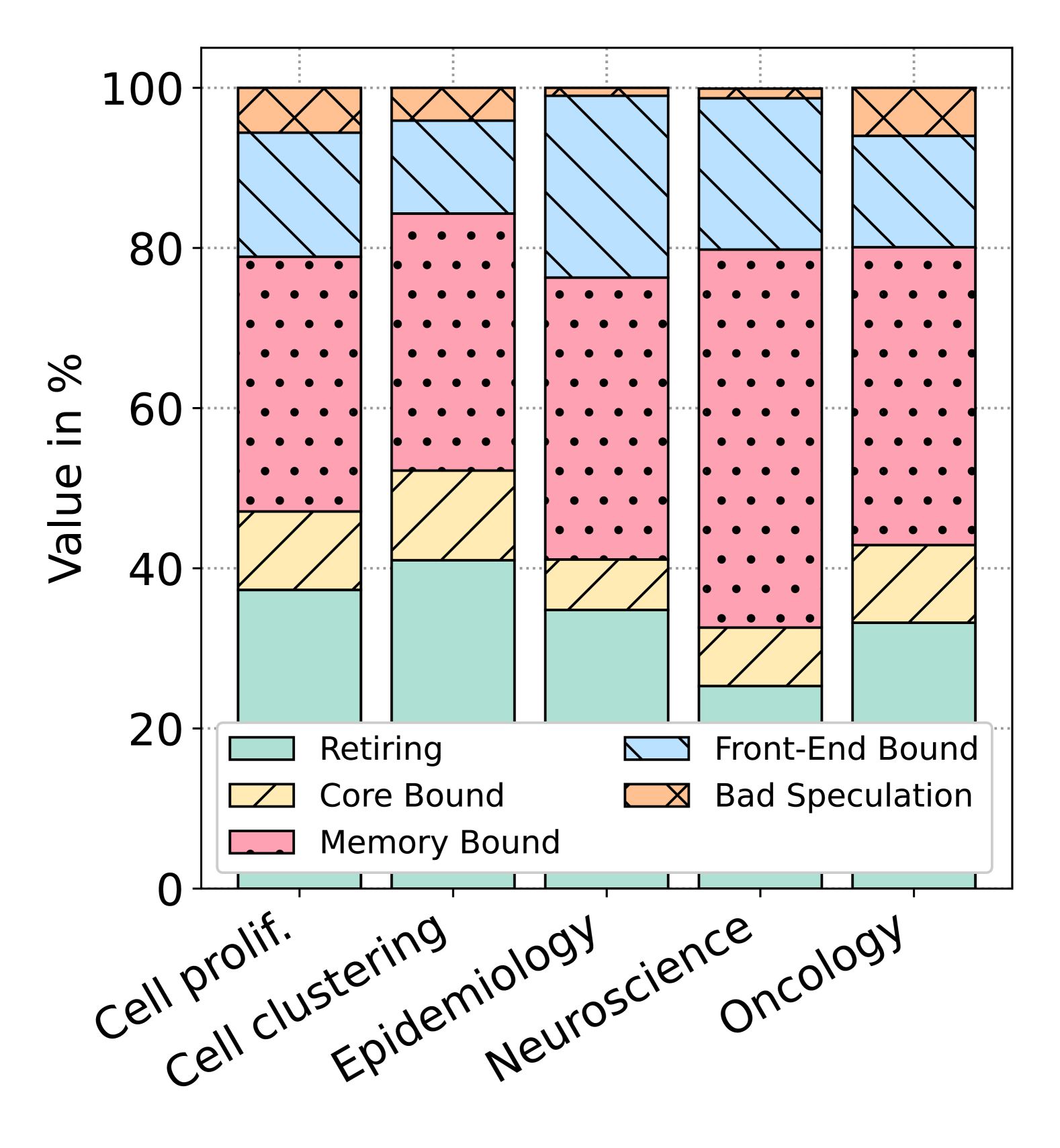
?figurename? 5.6: Operation runtime breakdown (left) and microarchitecture analysis (right)

The majority of the runtime is spent in agent operations (median: 76.3%) which subsumes, among others, the execution of behaviors, calculation of mechanical forces, discretization, and detection of static regions. Rebuilding the uniform grid environment at every time step is the second biggest runtime contributor, 4.09–36.5% (median: 18.0%). The epidemiology use case considers a wider environment that manifests itself in an increased update time. The average cost of agent sorting in its optimal setting (see Figure 5.14) is 0.180%–6.33%. Since adding and removing agents is parallelized, iterations’ setup and tear down consume only 2.66% (max) of the execution time.

In the microarchitecture analysis, we observe that the benchmark simulations are primarily memory-bound. We lose between 31.8 and 47.2% of processor pipeline slots because the operands are not available.

5.6.4 Runtime and Space Complexity

We analyze the runtime and memory consumption of BioDynaMo on System B by increasing the number of agents from $10^{3}$ to $10^{9}$ for each simulation (Figure 5.7). With one thousand agents, the execution time for one iteration is on average 1.21 ms and increases only slightly until $10^{5}$ agents (2.80ms). From there on, runtime increases linearly to one billion agents in which one iteration takes between 6.41 and 38.1 seconds to execute. A similar trend can be observed for the memory consumption of BioDynaMo (using double-precision floating point values), which remains below $1.60$ GB until $10^{6}$ agents and increases linearly to a maximum between $245$ and $564$ GB.

The number of agents that BioDynaMo can simulate is not fundamentally limited to one billion. The maximum depends only on the available memory of the underlying hardware and the tolerable execution time.

?figurename? 5.7: Average runtime per iteration and memory consumption analysis as the number of agents varies from $10^{3}$ to $10^{9}$

.

5.6.5 Comparison with Biocellion

We compare BioDynaMo with Biocellion [7], an agent-based framework for tissue models optimized for performance. We implement the cell sorting simulation presented in the Biocellion paper (Section 3.1) in BioDynaMo and use identical model parameters. The visualization of the BioDynaMo simulation with 50k cells (Figure 5.8(a)) demonstrates a good agreement with the Biocellion results in Figure 3a in [7].

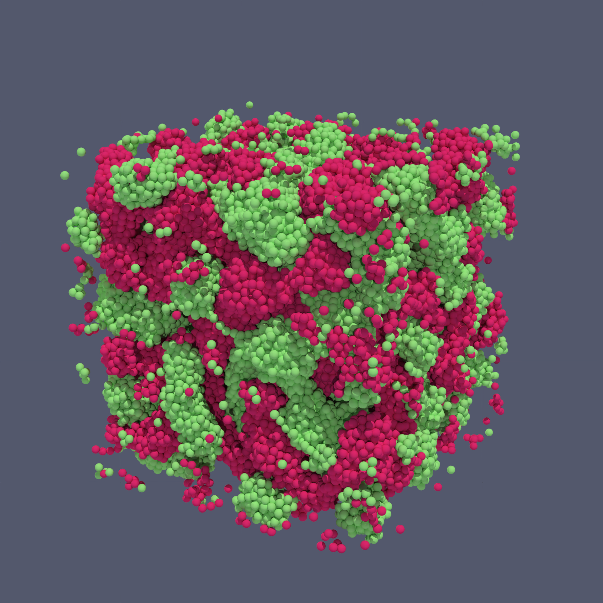
(a)

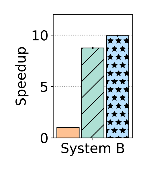
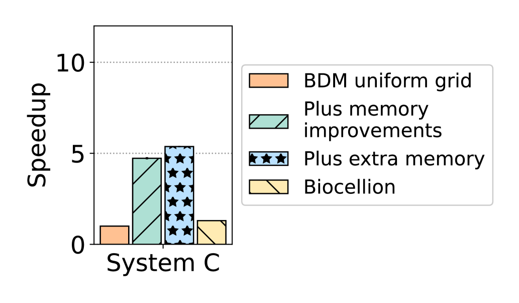
(b)

?figurename? 5.8: (a) Final simulation state after executing the Biocellion cell sorting model on BioDynaMo. (b) Performance evaluation of the BioDynaMo optimizations with a model with 28.6 million cells on System B (left) and System C limited to 16 physical CPU cores (right). The Biocellion paper [7] provides only a performance measurement for the latter benchmark.

Since we do not have access to the Biocellion code, because it is proprietary software, we compare BioDynaMo to the performance results provided in [7]. First, we replicate the benchmark with 26.8 million agents using 16 CPU cores. For Biocellion, Khang et al. [7] used a system with two Intel Xeon E5-2670 CPUs with 2.6 GHz. We execute BioDynaMo on System C with a comparable CPU and limit the number of CPU cores to 16 to ensure a fair comparison. We observe that BioDynaMo is 4.14$\times$ faster than Biocellion. BioDynaMo executes one iteration in 1.80s (averaged over 500 iterations), while Biocellion requires 7.48s.

Second, we consider the Biocellion benchmark in which Kang et al. executed 1.72 billion cells on a cluster with 4096 CPU cores (128 nodes with two AMD Opteron 6271 Interlago 2.1 GHz CPUs per node). We execute the BioDynaMo simulation with the same number of cells on a single node (System B). Although BioDynaMo requires 26.3s per iteration, which is 5.90$\times$ slower than Biocellion, BioDynaMo uses 56.9$\times$ fewer CPU cores. Therefore, we conclude that the performance per CPU core of BioDynaMo is 9.64$\times$ more efficient than Biocellion. We repeat the experiment with 281.4 million cells to verify the last observation. Biocellion requires 4.37s per iteration (extracted from Figure 3b in [7]) using 21 nodes with a total of 672 CPU cores. The BioDynaMo simulation on System B with 72 CPU cores runs in almost identical 4.24s per iteration. This result confirms our observation that BioDynaMo is an order of magnitude more efficient than Biocellion.

We evaluate the impact of our optimizations to provide insights into the question of why BioDynaMo processes 4.14$\times$ more agents per CPU core in the first benchmark and 9.64$\times$ in the second. Therefore, we execute the relevant optimizations with 26.8 million cells on System C limited to 16 CPU cores and System B with 72 CPU cores. Figure 5.8(b) shows that the difference can largely be explained by the memory optimizations having a more significant impact on machines with higher CPU core count.

5.6.6 Comparison with Cortex3D and NetLogo

We also compare with capable single-thread tools to evaluate the parallel overhead of the BioDynaMo implementation [427]. We choose Cortex3D [39] due to its similarity with the neuroscience features of BioDynaMo and select NetLogo [186] as a representative for an easy-to-use general-purpose tool. We extend the experiments from [188] by analyzing the impact of the presented performance improvements and comparing the memory consumption. This benchmark uses different simulation parameters for agents, diffusion volumes, and iterations, than shown in Table 5.1. The first four benchmarks in Figure 5.9 are small-scale benchmarks using between 2k and 30k agents and 0–128k diffusion volumes. These benchmarks run for 100–1000 iterations and only use one thread because Cortex3D and NetLogo are not parallelized. The “epidemiology (medium-scale)” benchmark contains 100k agents and uses 144 threads. NetLogo only benefits from parallel garbage collection in this scenario. In the “BioDynaMo standard implementation”, all optimizations are turned off, and the kd-tree environment is used.

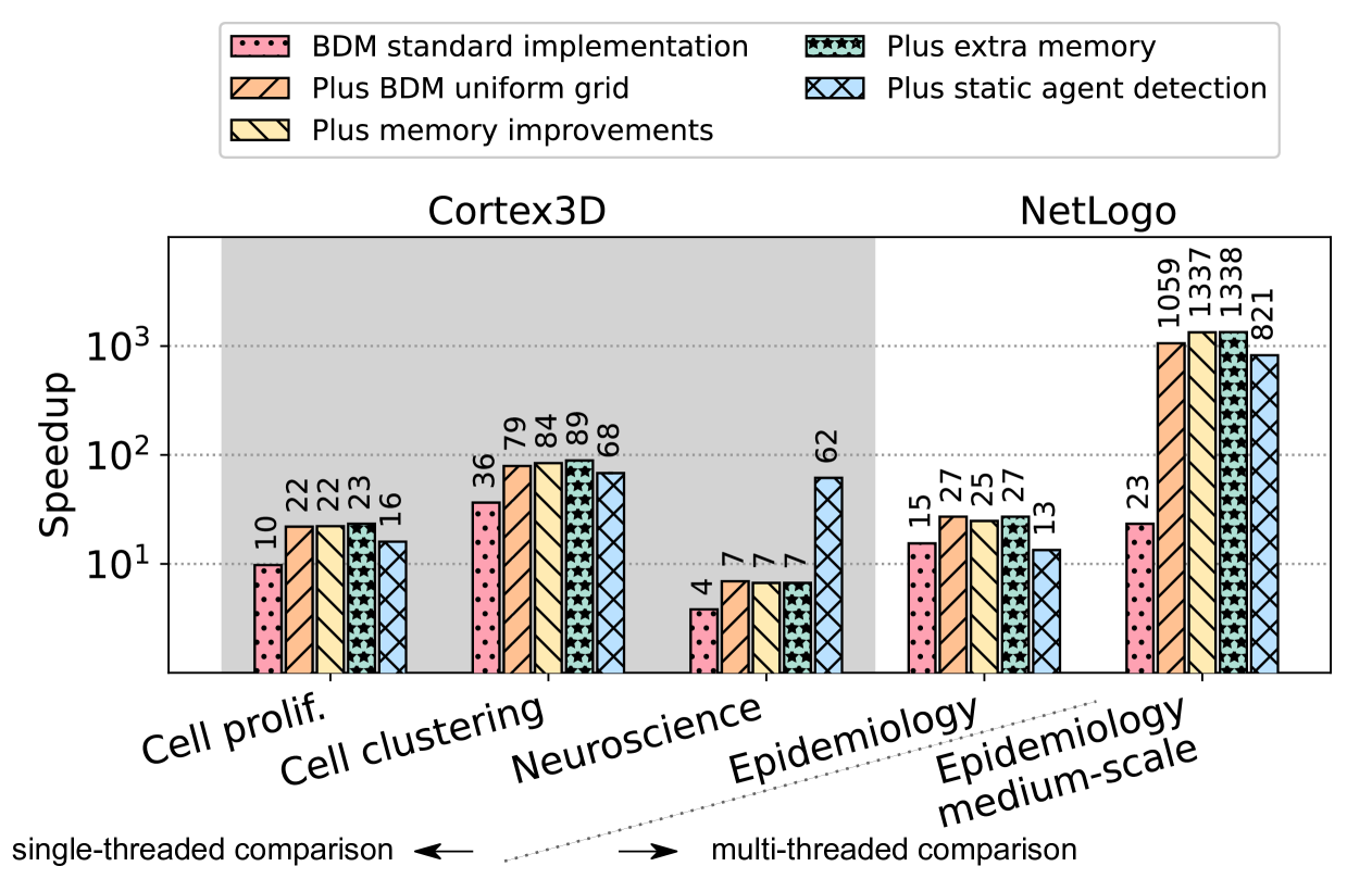
?figurename? 5.9: Performance comparison with Cortex3D and NetLogo after the optimizations are progressively switched on.

We make the following observations. For the small-scale simulations using one thread, BioDynaMo achieves a speedup of up to 78.8$\times$ while using 2.49$\times$ less memory. We observe three orders of magnitude speedup and two orders of magnitude reduction in memory consumption for the medium-scale benchmark in which all threads were used.

The median speedup of the BioDynaMo standard implementation is 15.5$\times$. The optimized uniform grid of BioDynaMo boosts performance in all benchmarks (median: 2.18$\times$) but has the most significant impact if parallelization is used (45.5$\times$). Memory layout optimizations improve the runtime of medium-scale simulations by 26.2%, but not for small-scale ones. The memory layout optimizations comprise the NUMA-aware iteration (Section 5.4.1), agent sorting and balancing (Section 5.4.2), and memory allocator (Section 5.4.3). Due to the interdependency between these individual optimizations, we subsumed them into one category. Similarly, extra memory usage during the agent sorting and balancing stage (Section 5.4.2) has only a slight performance impact (median speedup: 4.82%). However, the static region optimization dramatically improves the performance in the neuroscience use case (speedup 9.22$\times$). Although the mechanism’s overhead reduces the speedup for simulations without static regions, this is not problematic. The modeler usually knows this characteristic a priori and only enables the mechanism if static regions are expected (see parameter detect_static_agents).

5.6.7 Optimization Overview

We assess the performance of the presented optimizations using larger-scale simulations (Table 5.1) by enabling optimizations step-by-step (Figure 5.10). The baseline in this comparison is the BioDynaMo standard implementation introduced in Section 5.6.6.

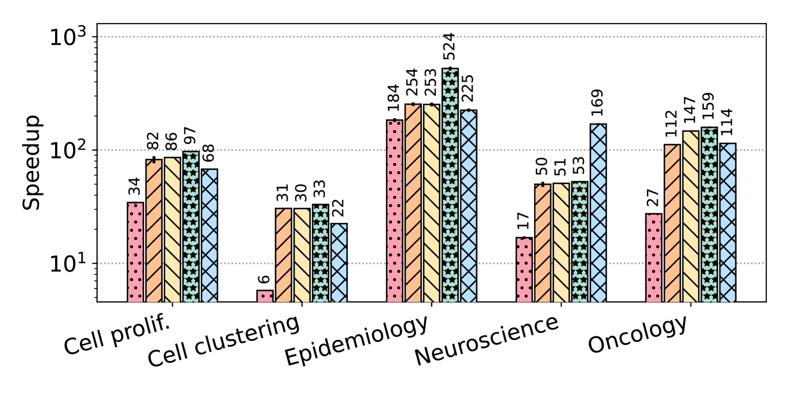
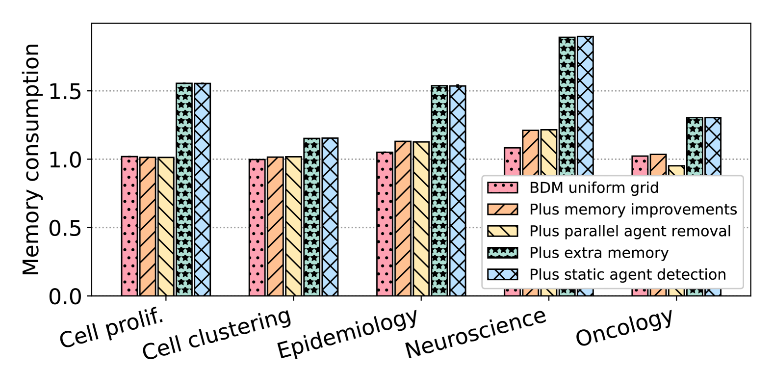
?figurename? 5.10: Speedup (top) and memory consumption (bottom) compared with the BioDynaMo standard implementation after the optimizations are progressively switched on. The legend is shared between the plots.

We make the following observations. The BioDynaMo optimizations improve overall performance between 33.1$\times$ and 524$\times$ (median: 159$\times$). These benchmarks confirm the speedup of BioDynaMo’s optimized uniform grid that we observed in comparison with Cortex3D and NetLogo. For these larger-scale simulations, the magnitude of the speedup increases up to 184$\times$ with a median of 27.4$\times$. A similar observation can be made for the static region detection mechanism, albeit with reduced magnitude (speedup: 3.22$\times$). The main difference between the comparison with Cortex3D and NetLogo and this benchmark is the impact of the memory layout optimizations of agents and behaviors and the usage of extra memory during agent sorting. The maximum speedup is up to 5.30$\times$ (median: 2.96$\times$) and up to 2.07$\times$ (median: 1.09$\times$), respectively. Only the Biocellion benchmark in Figure 5.8(b) shows a bigger impact.

The simulation time of the oncology use case, the only benchmark that removes agents from the simulation is reduced by 31.7% using the “parallel removal” optimization described in Section 5.3.2. The optimizations increase the median memory consumption by a mere 1.77%, which increases to 55.6% by enabling the use of extra memory during agent sorting.

5.6.8 Scalability

We evaluate the scalability of BioDynaMo using the complete simulations lasting between 288 and 1000 iterations and perform a strong and weak scaling analysis with different optimizations enabled. The strong scaling analysis is performed with ten iterations.

Figure 5.11(a) illustrates the excellent scalability of BioDynaMo for complete simulations (i.e., executing all iterations). The speedup using 72 physical cores with hyperthreading enabled is between 60.7$\times$ and 74.0$\times$ (median 64.7$\times$) compared to serial execution. Section 5.6.6 shows that BioDynaMo with one CPU core is more than 23$\times$ faster than Cortex3D. If we combine this result with the scalability analysis, which shows that BioDynaMo with 72 CPU cores is more than 60$\times$ faster than one CPU core, we can conclude that BioDynaMo is up to three orders of magnitude faster than Cortex3D.

Figures 5.11(c)–5.11(g) show the strong scaling analysis for each benchmark simulation with ten iterations after progressively switching on the presented optimizations. The left column shows the speedup with respect to a single-thread execution, and the right column presents the average runtime in milliseconds to highlight the absolute differences between various optimizations and the reduction in runtime with increasing threads. We make the following observations. The BioDynaMo standard implementation scales poorly due to the serial build of the kd-tree environment, which is improved considerably by using BioDynaMo’s optimized uniform grid (Section 5.3.1). The presented memory optimizations (Section 5.4) fully achieve their desired effect and allow BioDynaMo to scale across NUMA domains and high CPU-core counts.

We make the same observations for the weak scaling analysis (Figure 5.12), in which the number of agents is increased proportionally to the number of threads. Under ideal conditions, we expect the runtime to remain constant for each thread count. Also for this benchmark, we switch on the optimizations one after the other to highlight their impact on the runtime and see significant improvements over the baseline.

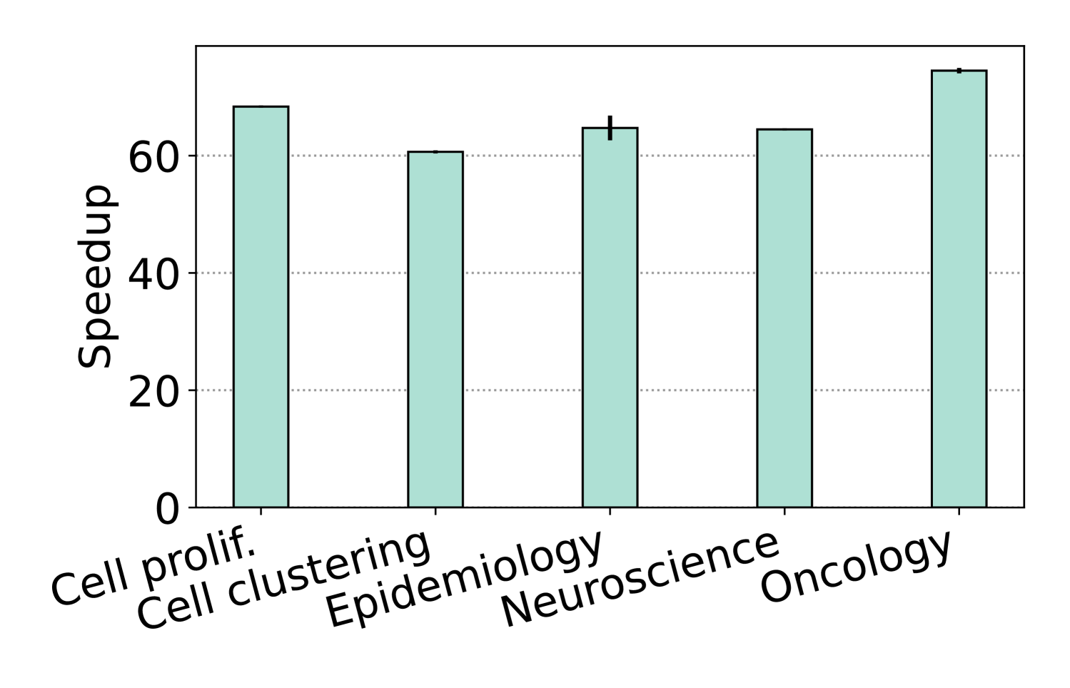
(a) Whole simulation scalability

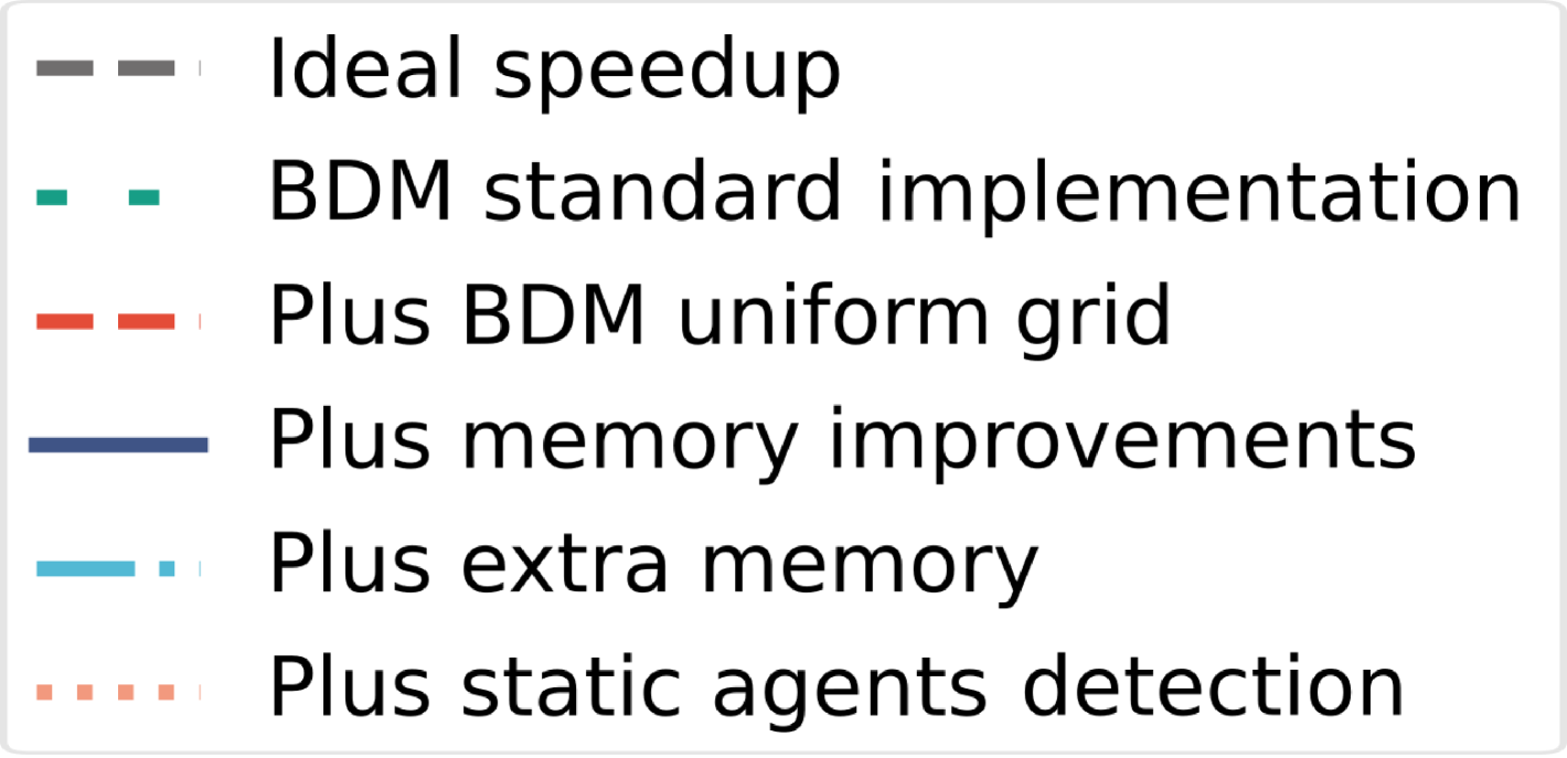
(b) Legend for (c)–(g)

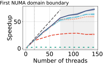
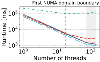
(c) Cell proliferation

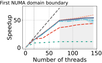
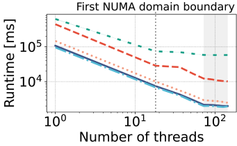
(d) Cell clustering

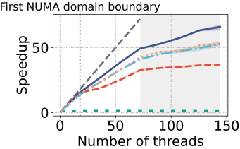
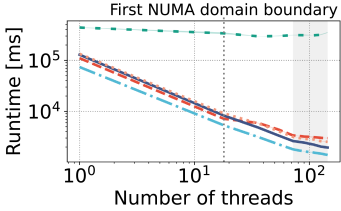
(e) Epidemiology

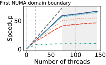
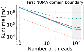
(f) Neuroscience

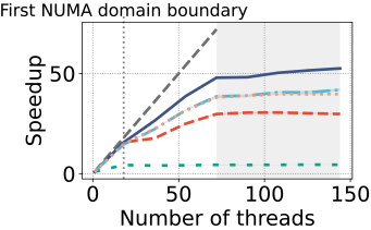
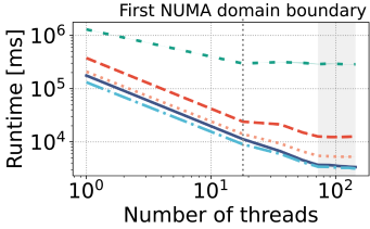
(g) Oncology

?figurename? 5.11: (a) Simulation scalability using the whole simulation. (b–g) Detailed strong scaling analysis using only ten time steps. The left column shows the speedup with respect to a single-thread execution, while the right column presents the total runtime.

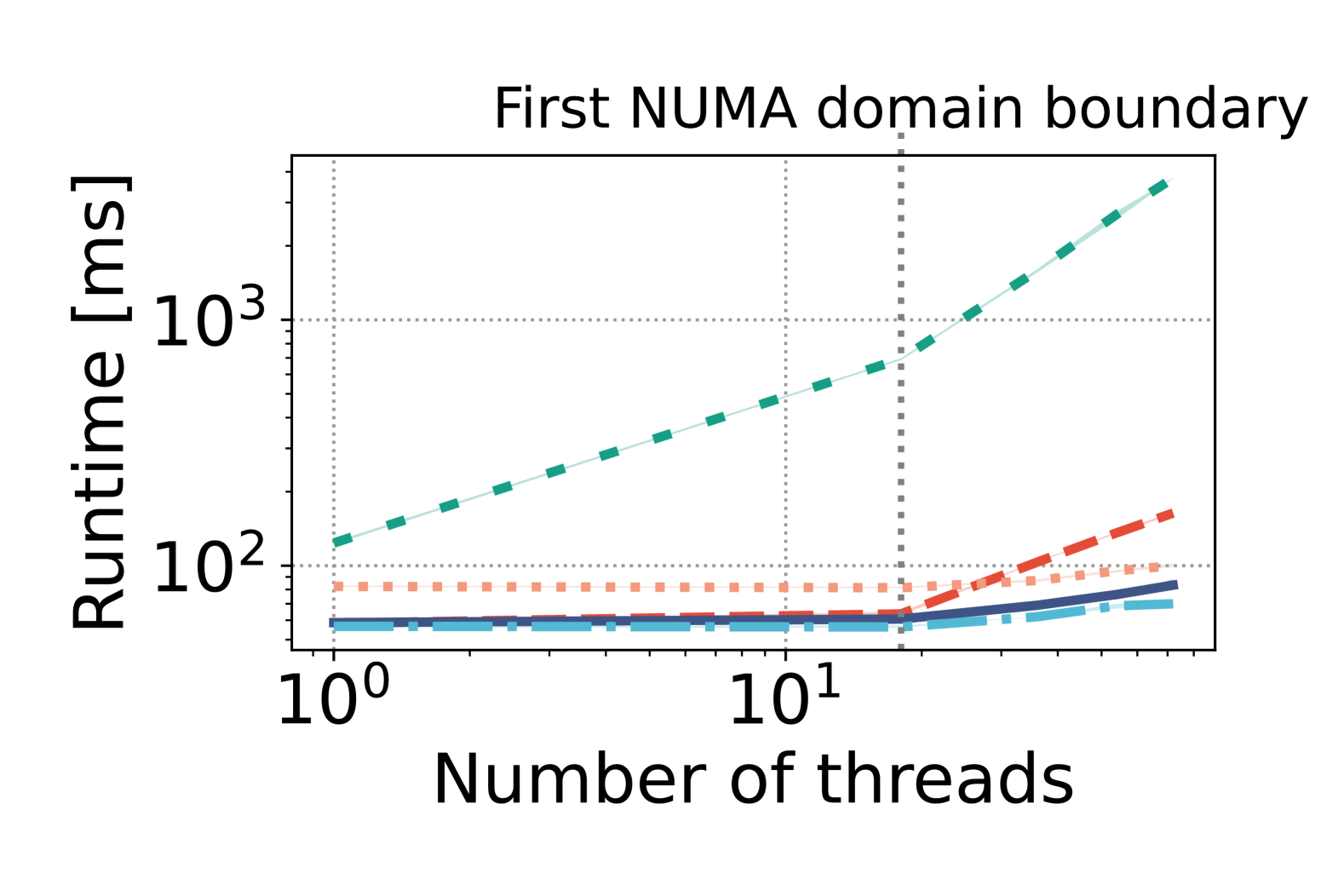
(a) Cell proliferation

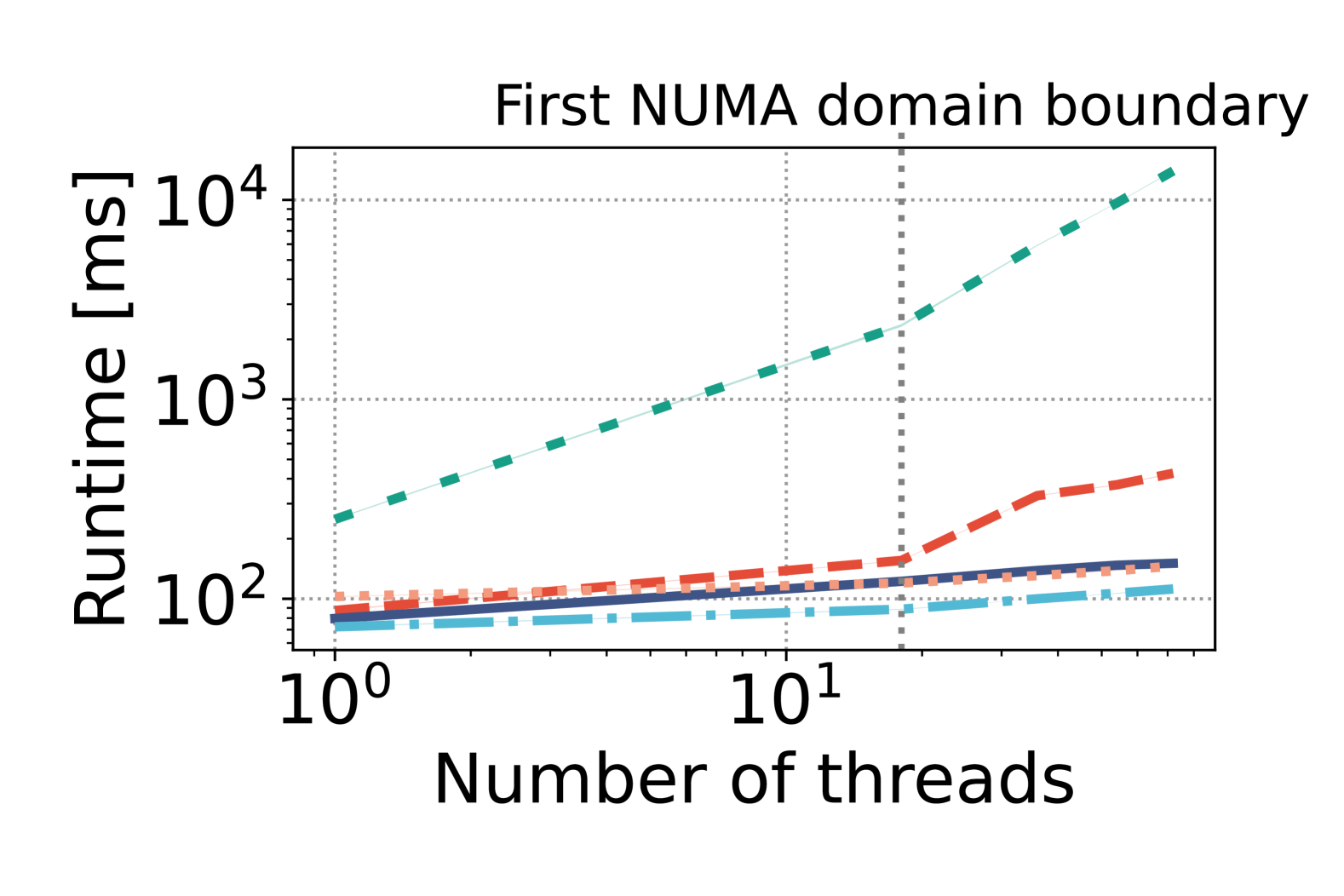
(b) Cell clustering

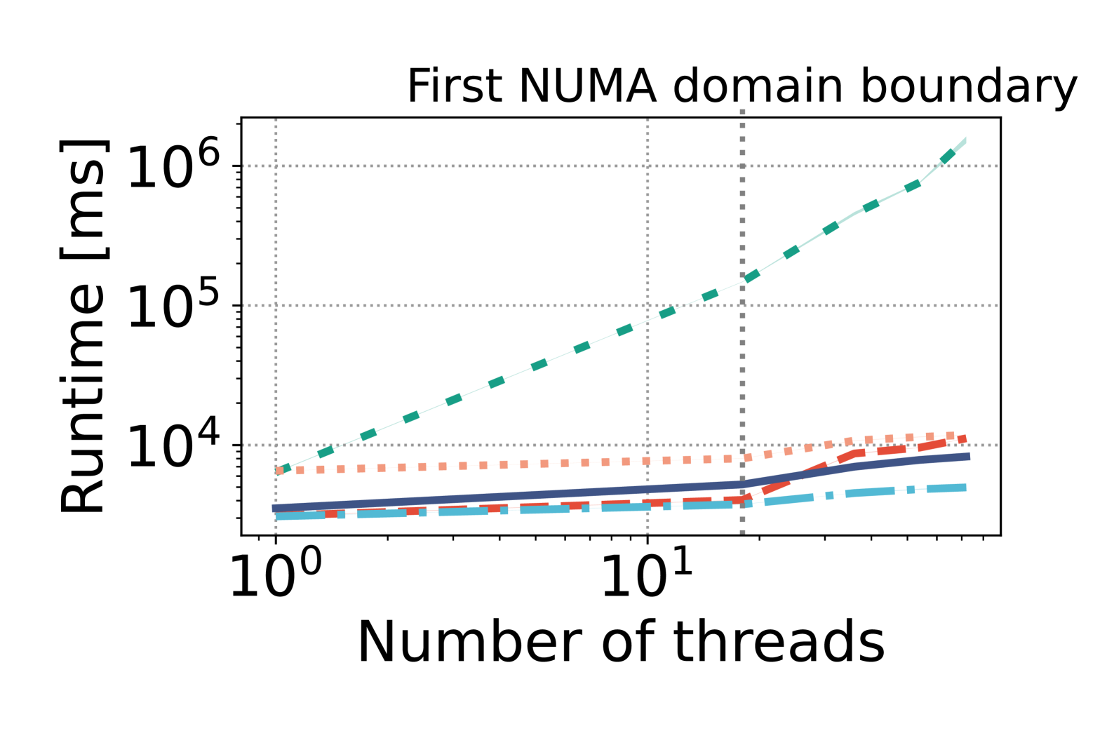
(c) Epidemiology

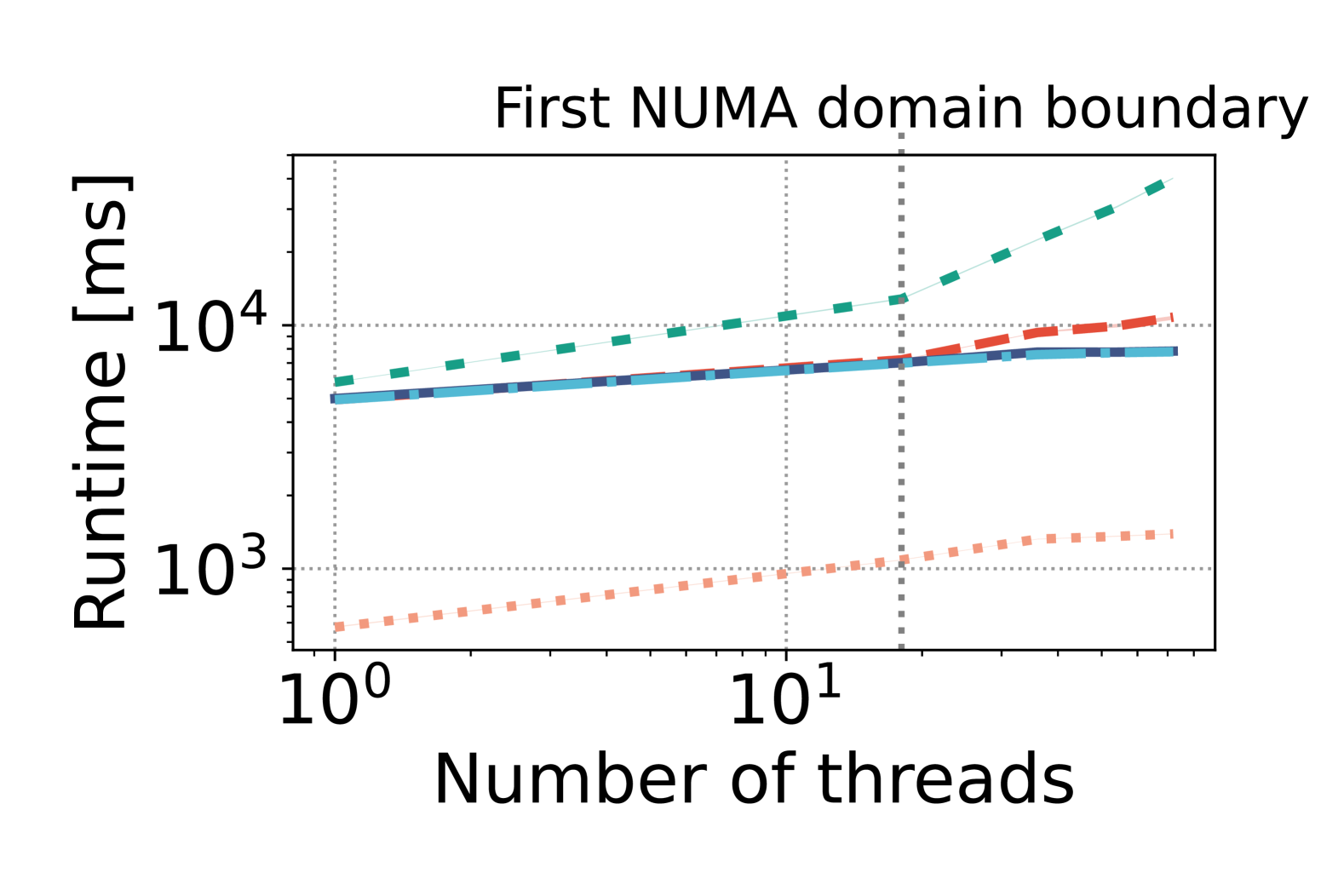
(d) Neuroscience

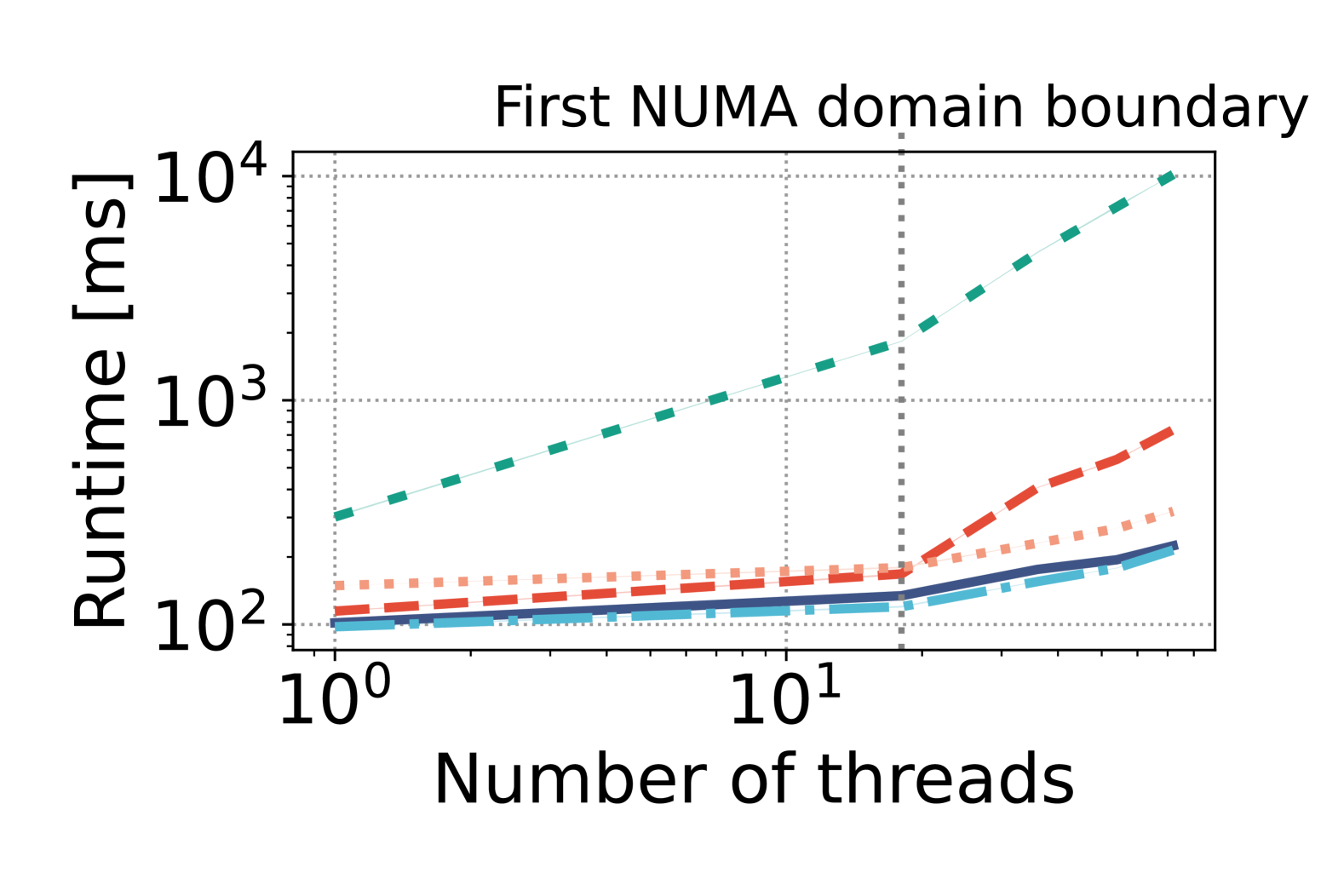
(e) Oncology

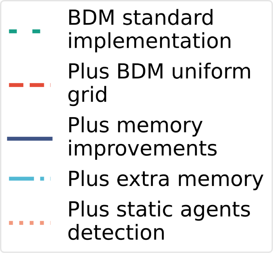
(f) Legend for (a)–(e)

?figurename? 5.12: (a–e) Weak scaling analysis using the whole simulation. (f) Legend shared between the figures (a–e).

5.6.9 Neighbor Search Algorithm Comparison

Figure 5.13 compares three different neighbor search algorithms: BioDynaMo’s uniform grid, UniBN’s octree [339], and the kd-tree from nanoflann [422]. To ensure a fair comparison, we turned off agent sorting for all algorithms because it is currently only implemented for the uniform grid. We validate our choice for the octree bucket size and nanoflann depth parameter and observe that the used parameters are within 4.20% of the optimum runtime. The left column in Figure 5.13 shows the result for four NUMA domains and 144 threads, while the right column shows results for one NUMA domain and 18 threads. We analyzed four properties of these radial neighbor search methods: runtime impact on the whole simulation, build and search time of the index, and memory consumption (Figure 5.13). We measure the search time indirectly by comparing the agent operation runtimes. This operation contains the initial neighbor searches and thus provides information on how fast searches are executed.

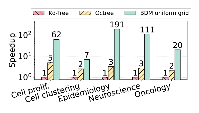
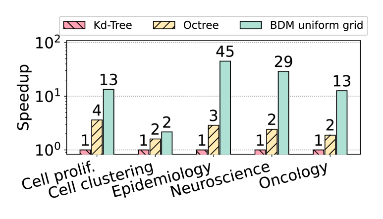
(a) Whole simulation

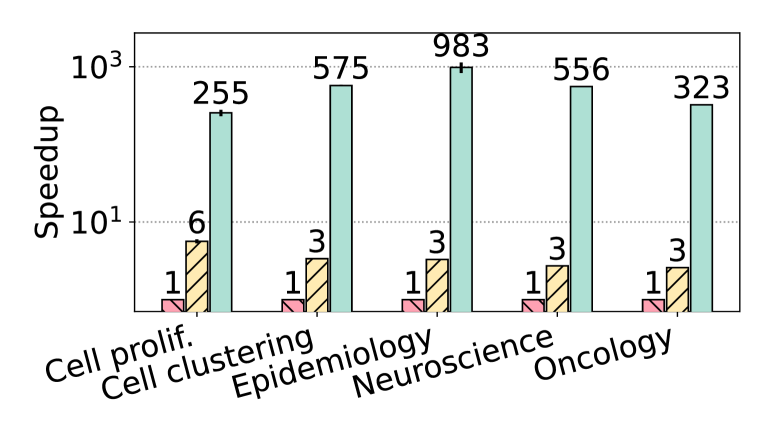
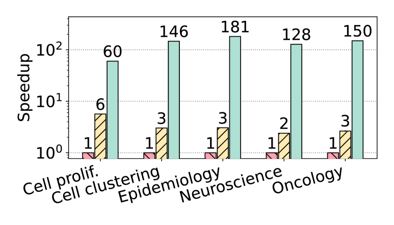
(b) Build time

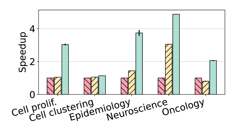
(c) Search time (indirect)

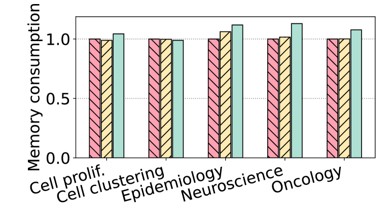
(d) Memory consumption

?figurename? 5.13: Neighbor search algorithm comparison (left column: four NUMA domains and 144 threads, right column: one NUMA domain and 18 threads). The legend is shared between the plots.

The BioDynaMo uniform grid implementation shows its benefits not only in the pure build time comparison but also in the full simulation analysis. Although a significant build time difference in comparison to the kd-tree and octree is expected (because the build process is serial), the magnitude between 255 and 983$\times$ on four NUMA domains is surprising. The uniform grid outperforms the other algorithms also during the search stage for all simulations.

Simulations using BioDynaMo’s uniform grid implementation are up to 191$\times$ faster than the kd-tree implementation while consuming only 11% more memory in the worst case.

5.6.10 NUMA-Aware Iteration

We evaluate the individual performance impact of NUMA-aware iteration (Section 5.4.1). In the other benchmarks, this optimization was included in the “memory layout optimization” group. We compare the simulation runtime with all optimizations enabled, to executions in which “NUMA-aware iteration” is turned off. This benchmark shows that this mechanism reduces the runtime between 1.07$\times$ and 1.38$\times$ (median: 1.30$\times$).

5.6.11 Agent Sorting and Balancing

This section evaluates the impact of agent sorting and balancing (Section 5.4.2) on the simulation runtime for one and four NUMA domains. To this extent, we perform a parameter study with varying agent sorting frequencies for each simulation. Figure 5.14 shows the speedup for four NUMA domains (left) and one NUMA domain (right). The baselines in both cases are simulations without agent sorting. An agent sorting frequency of one means that the operation is executed in every iteration; similarly, a frequency of ten would mean that the operation is executed every ten iterations.

Load balancing of agents among NUMA domains greatly impacts performance even on systems without NUMA architecture. This stems from the fact that the agent sorting operation also aligns agents that are close in space also in memory.

The oncology and cell clustering simulations benefit most of this performance improvement (peak speedup of 5.77 and 4.56$\times$ for four NUMA domains). Both simulations are initialized with a random distribution of agents. Although the epidemiology simulation is also initialized randomly, its agents also move randomly with large distances between iterations. This behavior reduces the alignment improvements significantly (peak speedup 1.14$\times$ for four NUMA domains). The cell proliferation simulation is initialized with a 3D grid of cells, which improves the alignment compared to the worst-case random initialization. Therefore, the maximum obtained speedup is reduced to 1.82$\times$ (four NUMA domains). Suppose we change the initialization of the cell proliferation simulation to random, the maximum speedup increases to 4.68$\times$. This optimization performs below average for the neuroscience simulation. This simulation only has an active growth front, while the remaining part remains static. The static agent detection mechanism exploits this fact and avoids calculating mechanical forces for the static regions. Therefore, the number of neighbor accesses is significantly reduced, and thus the benefits of aligned agents. If static region detection is disabled, agent sorting and balancing improve the runtime by 3.80$\times$ at a frequency of 20.

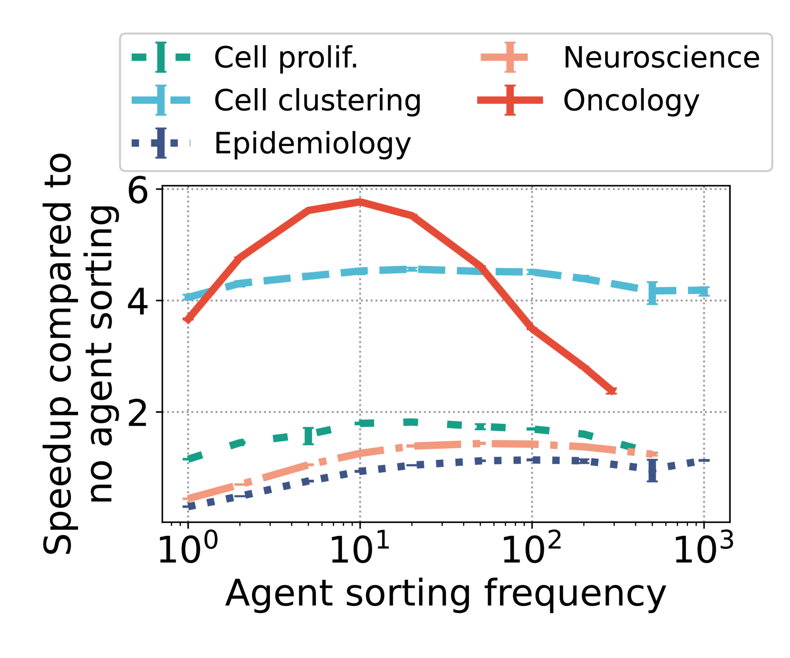
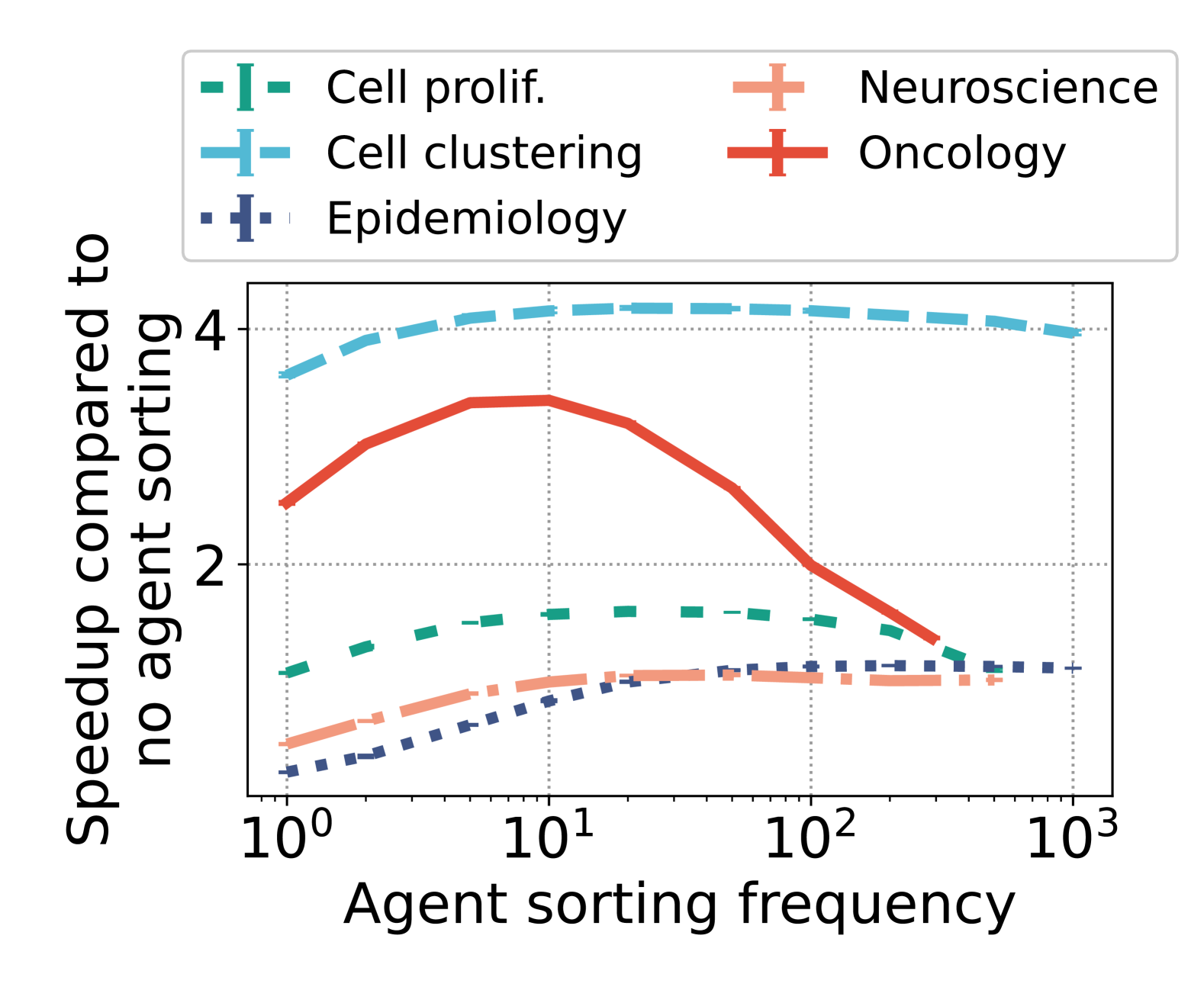
?figurename? 5.14: Agent sorting and balancing speedup for different execution frequencies (left: four NUMA domains and 144 threads, right: one NUMA domain and 18 threads).

5.6.12 BioDynaMo Memory Allocator

To evaluate the performance of the BioDynaMo memory allocator, we compare it with glibc’s version of ptmalloc2 [428] and jemalloc [426] using our five benchmark simulations. A comparison with tcmalloc [429] was impossible due to deadlock issues that we discovered during benchmarking. Only the epidemiology use case uses additional memory during agent sorting and balancing. Since the BioDynaMo memory allocator only covers agents and behaviors, we need to use another allocator for the remaining objects.

This requirement results in four tested configurations per simulation, as illustrated in Figure 5.15. The BioDynaMo memory allocator improves the overall simulation runtime up to 1.52$\times$ over ptmalloc2 (median: 1.19$\times$) and up to 1.40$\times$ over jemalloc (median 1.15$\times$). The allocator consumes 1.41% less memory than ptmalloc2 and 2.43% less memory than jemalloc on average.

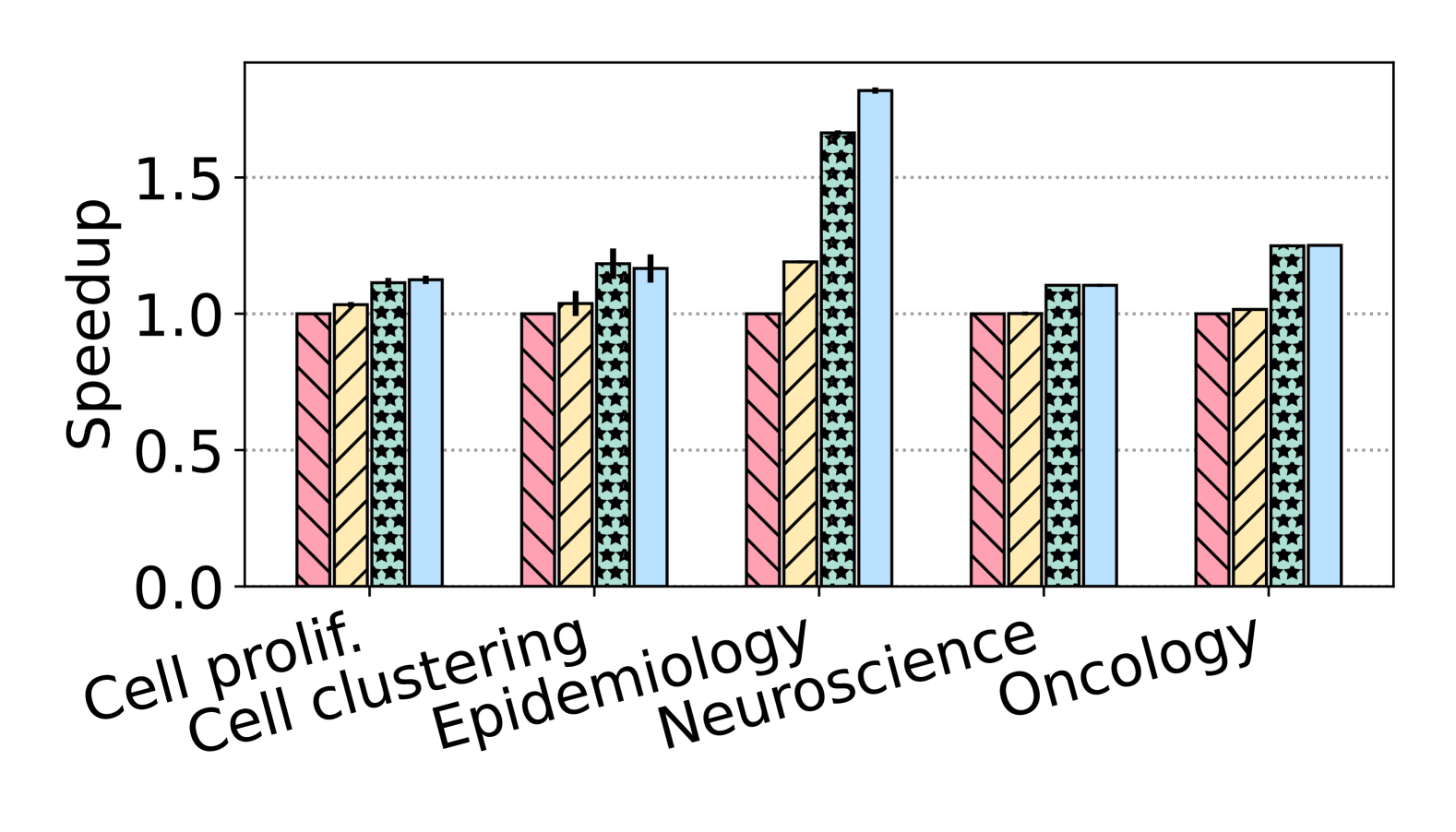
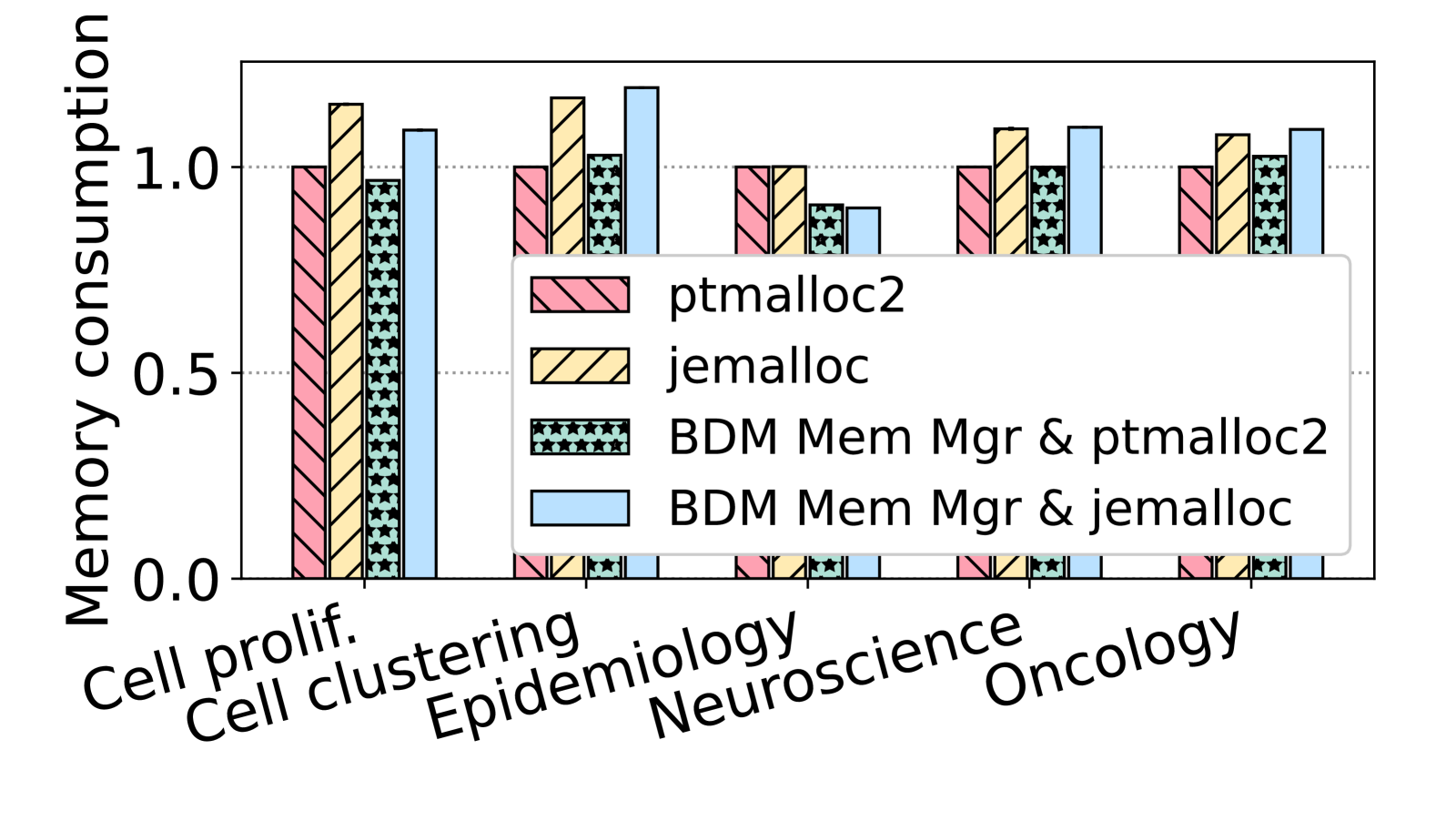
?figurename? 5.15: Memory allocator comparison (left: speedup, right: memory consumption). The legend is shared between the plots.

5.6.13 Visualization

This section evaluates the performance of the visualization integration which comprises the export of visualization files and rendering. We compare the performance of the file export on four dimensions. We distinguish between different data access methods (zero-copy, copy, and cache), storage location (SSD and in-memory file system [DRAM]), number of exported agent attributes (all attributes vs. required ones), and investigate the impact of file compression. The distinction between data access methods is specific to the file export. Therefore, the rendering evaluation has only three comparison dimensions.

Figure 5.16 shows the speedups for the visualization operation for the cell clustering and neuroscience use case. The baseline does not use the parallel file exporter and compression, and exports all agent attributes. The left column shows the file export and the right column the rendering results.

We make the following observations. The parallel file writers speedup the export between 9$\times$ and 19$\times$. Although compression reduces the file size between 1.62$\times$ and 3.7$\times$ the costs outweigh the benefits on our test system. This result might change for slower hard drives. Exporting required agent attributes on-demand reduces the file size by 2.47$\times$ and 2.67$\times$. The caching data access mode performs best for the in-memory file system and the cell clustering benchmark, while the differences for the neuroscience use case are minimal. The differences depend on the memory access pattern and computational intensity of the workload. Thus, bigger differences might be observed if this mechanism is used to integrate other third-party applications. As expected writing files to the in-memory file system is faster due to the higher bandwidth compared to the SSD.

In the rendering stage, no significant difference between compressed and uncompressed files, and DRAM and SSD could be observed. Also the difference between files that contain all agent attributes and files that contain the required ones can be observed. We attribute this effect to the columnar storage of the file format.

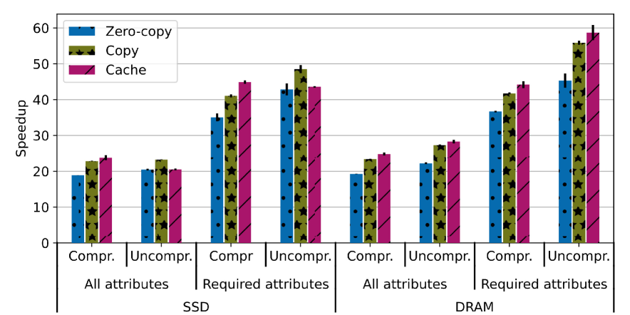
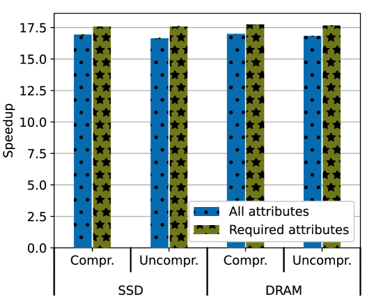
(a) Cell clustering

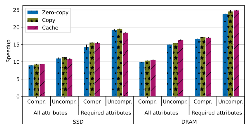
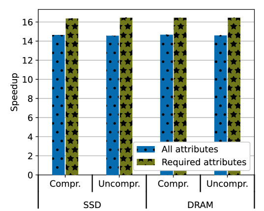
(b) Neuroscience use case

?figurename? 5.16: Visualization performance analysis. Left column: Speedups of the visualization operation using different parameters. Right column: Speedup of the rendering stage.

5.6.14 Alternative Execution Modes

This section evaluates the slowdown and memory consumption of different execution modes presented in Section 5.2.1 compared to BioDynaMo’s default settings. These results are shown in Figure 5.17. The copy execution context does not support the modification of neighbors yet. Therefore, this comparison is missing for the neuroscience use case.

As expected, row-wise iteration and randomization have the same memory consumption as BioDynaMo in its default setting. Up to 1.67$\times$ more memory is needed for the copy execution context to store the temporary agents. Row-wise execution is up to 2.67$\times$ slower (median: 1.27$\times$) due to poor temporal cache utilization and increased synchronization overhead. Locks must be acquired and released for each operation instead of once. The copy execution context slows down execution by 1.49$\times$ (median) because every agent is duplicated before it is processed. Randomization counteracts the memory layout improvements and hence degrades median performance by 3.97$\times$.

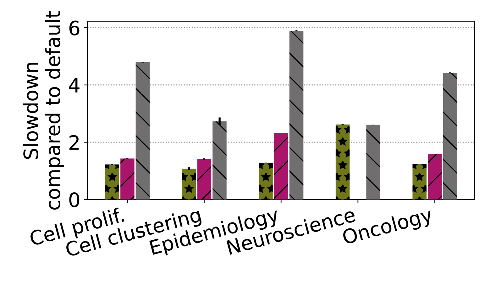
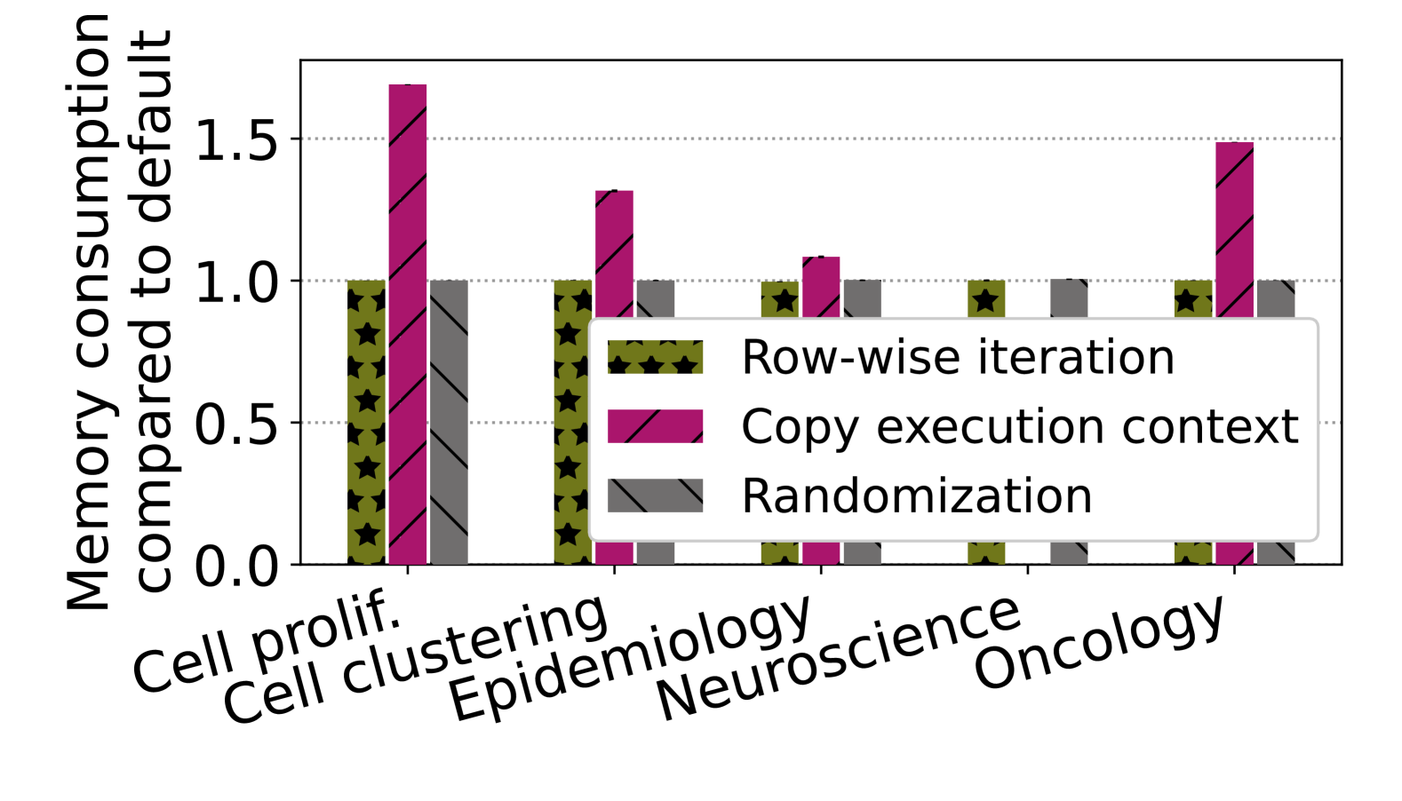
?figurename? 5.17: Comparison of alternative execution modes compared to BioDynaMo’s default settings (left: slowdown, right: memory consumption). The legend is shared between the plots.

5.7 Conclusion and Future Work

This chapter presents a novel agent-based simulation engine optimized for high performance and scalability. BioDynaMo enables not only larger-scale simulations, but also helps researchers of small scale studies with accelerated parameter space exploration, and faster iterative development.

We identify general agent-based performance challenges and provide six solutions to maximize parallelization, reduce memory access latency and data transfers, and avoid unnecessary work. These solutions are transferable and can be used to accelerate other agent-based simulation tools.

We present a comprehensive performance analysis to provide insights into the agent-based workload and to give our users a better understanding of BioDynaMo’s capabilities. We find that on our system, the presented optimizations improve performance up to 524$\times$ (median 159$\times$) and allow BioDynaMo to scale to 72 physical processor cores with a parallel efficiency of 91.7%. A comparison with state-of-the-art tools shows that BioDynaMo is up to three orders of magnitude faster. These performance characteristics enable simulations with billions of agents, as demonstrated in our analysis.

Our performance optimizations, which are effective on machines with one or more NUMA domains, are an important stepping stone towards a distributed simulation engine with a hybrid MPI/OpenMP design. Ongoing work focuses on realizing this distributed simulation engine capable of dividing the computation among multiple nodes to push the boundaries of agent-based simulation even further.

?chaptername? 6 TeraAgent: A Distributed Simulation Engine for Simulating Half a Trillion Agents

6.1 Introduction

Agent-based modeling is a bottom-up simulation method to study complex systems. Early agent-based models, dating back as far as 1971, studied segregation in cities [22], flock of birds [167], and complex social phenomena [195]. These models follow the same three-step structure, although the studied systems differ widely. First, the researcher has to define what the abstract term agent should represent. In the flock model from Craig Reynolds, an agent represents a bird. The bird has a current position, and a velocity vector. Second, the researcher has to define the interactions between agents. For example, birds avoid collision, align their heading with neighbors, and try to stay close to each other. Third, the researcher has to define the starting condition of the simulation. How should the birds be distributed in space in the beginning? What are their values for the initial velocity, and parameter values for the three behaviors? Once all these decisions are made, the model is given to the simulation engine, which executes it for a number of iterations, or until a specific condition is met.

Agent-based models exhibit two characteristics: local interaction and emergent behavior. First, agents only interact with their local environment and do not have knowledge about agents that are “far” away. This characteristic makes a distributed execution feasible via spatial partitioning of the agents, which results in data exchanges across partitions at the bordering regions. Second, agent-based models show emergent behavior or in other words they demonstrate that: “the whole is more than the some of its parts”. To come back to the flock of birds example, the swarm dynamics were not programmed into the model, but arose solely through the interactions of the birds following the three behaviors.

Since these early success stories, agent-based models have been used in numerous domains including biology [8, 10, 23, 11, 24, 25, 26, 27, 28, 29, 30, 31, 32, 33, 34, 35, 36, 37, 38, 39, 40, 41, 42, 43, 13, 40, 44, 45, 46, 47, 48, 49, 50, 51, 52, 53, 54, 55, 56, 57, 58, 59, 60, 61], medicine [23, 11, 24, 25, 62, 63, 64, 65, 66, 67, 68, 69, 70, 71, 72, 73, 74, 75, 76, 77, 78, 79, 80, 81, 82, 83, 84, 85, 86], epidemiology [87, 88, 89, 90, 91, 92, 93, 94, 95, 96, 97, 98, 99, 100, 101, 102, 103, 104, 105, 106, 107, 108, 109, 110, 111, 112, 113, 114, 115, 116, 117], finance [122, 123], policy making [430] and many more [414, 146, 147, 148, 149, 150, 64, 151, 152, 153, 154, 155, 156, 157, 158, 159, 160, 161, 162, 163, 164, 165, 166]. These systems often comprise a very large number of agents. Especially biomedical systems (the human cortex consists of approximately 86 billion neurons [391]) or country-scale epidemiological simulations [87].

Enabling simulations on these scales requires an efficient, high-performance, and scalable simulation platform. Chapter 4 and 5, have demonstrated that our simulation platform BioDynaMo outperforms state-of-the-art simulators and is capable of simulating 1.7 billion agents on a single server. However, BioDynaMo only leverages shared-memory parallelism with OpenMP [417] and is therefore limited by the compute resources of one server. More precisely, researchers that use BioDynaMo are facing three critical restrictions:

• Limited simulation size and complexity. As demonstrated in Chapter 5 a server with 1TB of main memory—significantly larger than typical memory capacities found in today’s data centers—cannot support more than two billion agents.

• It is not feasible to integrate with third party software that is parallelized predominantely with MPI, because the resulting performance would be prohibitively slow. Examples include the lattice Boltzmann solver OpenLB [431] and the visualization tool ParaView [392], particularly the in-situ visualization mode [432] that eliminates the need to export files to disk.

• Limited hardware flexibility. Connecting less powerful hardware together may be more cost-effective than relying on a high-end server for large-scale simulations that surpass the capabilities of typical commodity servers.

Our goals are two fold.

Goal 1:

We address the afore listed performance restrictions by presenting TeraAgent a novel distributed simulation engine that is able to execute a single simulation on multiple servers by dividing the simulation space. Distributed execution requires the exchange of agent information between servers, to obtain the local environment for an agent update, or migrate agents to a new server. These exchanges comprise a serialization stage (packing agents into a contiguous buffer) and a transfer stage, which incur high performance and energy overheads. To alleviate such overheads, we address both stages with the following key improvements. First, we introduce a serialization mechanism for TeraAgent, tailored to the needs of agent-based simulations. Our serialization mechanism allows using the objects directly from the received buffer. Second, we extend the serialization mechanism with delta encoding and compression to exploit the iterative nature of agent-based simulations to minimize the required data transfers.

Goal 2:

Second, analogous to the OpenMP parallelization presented in Chapter 4, we incorporate the distribution into the platform, such that the additional parallelism is mostly hidden from the user. Thus, we support seamless model execution starting from laptops, workstations, and high-end servers [171] up to supercomputers and clouds without the need to modify the simulation code, for a wide range of simulations.

The main contributions of this chapter are:

• We present a novel distributed simulation engine called TeraAgent capable of simulating 501.51 billion agents and scaling to 84’096 CPU cores.

• We show that it is possible to make scale-out agent-based simulations practical by alleviating their data movement overheads across nodes via tailored serialization and delta encoding based compression.

• We present a novel serialization method for the agent-based use case, which significantly reduces the time spent on packing and unpacking agents during agent migrations and aura exchanges. We observe a median speedup of 110$\times$ for serialization and 37$\times$ for deserialization.

• We extend our serialization method to support delta encoding to reduce the amount of data that has to be transferred between servers, which reduces the message size by up to 3.5$\times$.

6.2 TeraAgent’s Distributed Simulation Engine

This section provides an overview of the required steps in distributed execution (Section 6.2.1), details the TeraAgent IO serialization mechanism (Section 6.2.2), presents our delta encoding scheme to reduce the amount of data that needs to be transferred (Section 6.2.3), explains implementation details (Section 6.2.4), and further improvements over BioDynaMo (Section 6.2.5).

6.2.1 Distribution Overview

Figure 6.1 shows an overview of the steps involved in the distributed execution of an agent-based simulation. The figure is simplified for a 2D simulation, but also applies for simulations in 3D. Figure 6.1A shows a simulation that is executed on two processes (ranks in MPI terminology [367]) that do not share their memory space. We apply a partitioning grid (consisting of partitioning boxes) on the simulation space to divide the space into mutually exclusive volumes corresponding to the number of ranks. It follows that each rank is authoritative of the assigned volume (or area in 2D) and the agents inside it. Figure 6.1B shows these regions in blue and green together with the interactions between the two ranks at the bordering regions. The specifics of these interactions, which happen in each simulation iteration are outlined below.

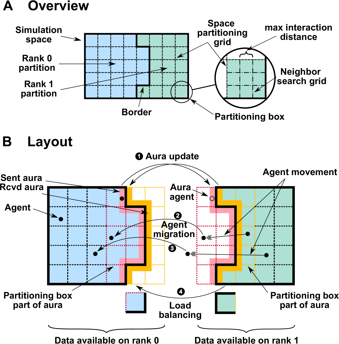
?figurename? 6.1: Distributed execution overview

Aura Update.

In this section, we focus on how agents close to the bordering region between two ranks interact with their local environment, which, for our purposes, consists only of other agents. In simulations conducted in Euclidean space, the local environment is defined by a radius centered around each agent. The modeler sets the radius value at the beginning of the simulation.

For agents located near the boundary between ranks, part of their local environment may reside on a different rank. Therefore, agents situated near these boundaries must have their data transmitted to neighboring ranks to enable the update to the next simulation iteration. Figure 6.1B illustrates the bordering region sent from rank 0 to rank 1 in red and yellow for the opposite direction. These areas are commonly referred to in the literature as aura, halo, or ghost regions. Consequently, these exchanges of data are known as aura updates.

It is important to note that the partitioning grid’s boxes can be larger than the maximum interaction distance of the agents. The zoomed-out detail in Figure 6.1A shows that, in this specific example, the partitioning boxes are three times larger than the maximum interaction distance. Consequently, regions outside this interaction distance do not need to be transferred. Therefore, the aura regions shown in red and yellow in Figure 6.1B are narrower than the partitioning box.

Agent Migration.

Agents that change their position might also move out of the locally-owned simulation space and must therefore be moved to the rank which is authoritative for the agent’s new position. For this scenario we have to distinguish two cases. First, the current rank can determine the destination rank itself because the new position lies inside a partitioning box that is locally available. Second, if the agent lies outside all locally-available partitioning boxes, a collective lookup stage is necessary to determine the rank which is authoritative for the position .

Load Balancing.

The current space partitioning might be adjusted during the simulation to avoid load imbalances between MPI ranks and a therefore suboptimal resource utilization.

6.2.2 Serialization

For all required steps presented in Section 6.2.1 (agent migration, aura updates, and load balancing), agents are moved or copied to other ranks. Serialization is necessary to pack agents and their attributes to a contiguous buffer which can then be sent with MPI.

We initially utilized ROOT I/O, because it is already used in BioDynaMo [188] for backing up and restoring whole simulations. ROOT serves as the main data analysis framework for high-energy physics [361]. ROOT’s serialization (called ROOT I/O) is used at CERN to store more than one exabyte scientific data from the large hadron collider experiments [433]. According to Blomer [362], ROOT I/O outperforms other serialization frameworks like Protobuf [363], HDF5 [364], Parquet [365], and Avro [366].

However, we observed that agent serialization was a significant performance bottleneck and made the following four observations.

First, ROOT I/O keeps track of already seen pointers during serialization. Thus, ROOT can skip over repeated occurrences of the same pointer and ensure that upon deserialization all pointers point to the same instance. TeraAgent does not need this feature, because BioDynaMo does not allow multiple agents having pointers to the same object. In the distributed setting, this would lead to further challenges, because the pointed object could be required on more than one rank and updates to this object would need to be kept in sync. We enable pointers to other agents with an indirection implemented in the smart-pointer class AgentPointer. An AgentPointer stores the unique agent identifier of the pointed agent and obtains the raw pointer from a map stored in the ResourceManager. Therefore, the serialization of AgentPointers reduces to the serialization of the unique agent identifiers. The current TeraAgent version only supports const AgentPointers to avoid merging changes from multiple ranks.

Second, we observe that deserialization takes a significant amount of time. Therefore, we analyze the design of Google’s FlatBuffer serialization library which provides “access to serialized data without parsing/unpacking” [434]. FlatBuffer serialization library even supports mutability, but is limited to changing the value of an attribute. For example, adding or removing an element from a vector is not supported.

Third, the current goal is to execute TeraAgent on supercomputers and clouds on machines with the same endianness. Thus, if the condition holds, there should not be any CPU cycles spent on endian conversions.

Fourth, ROOT I/O ensures that data that was captured and stored decades ago, can still be read and analyzed today. Schema evolution is therefore needed to deal with changes that occurred since the data was written. In TeraAgent, the transferred data exists only during the execution of the simulation, sometimes only for one iteration. In this time frame, the schema, i.e., the agent classes with their attributes do not change. Therefore, TeraAgent skips schema evolution to reduce the performance and energy overheads.

Based on these four observations, we design TeraAgent to avoid pointer deduplication, deserialization, endianness conversions, and schema evolution to alleviate the performance and energy overheads of agent serialization.

6.2.2.1 TeraAgent IO

Following one of the design principles of C++ “What you don’t use you don’t pay for” [435], we create a serialization method that take these four observations into account and thus avoids spending compute cycles on unnecessary steps.

Figure 6.2A shows an abstract representation of the objects in memory. Starting from a root object (e.g., a container of agent pointers), a tree structure can be observed, because multiple pointers to the same memory block are disallowed. The nodes of the tree are formed by contiguous memory blocks that were allocated on the heap. The given example could be interpreted as having a pointer to a container with three different agents, that have zero, one, and two attached behaviors.

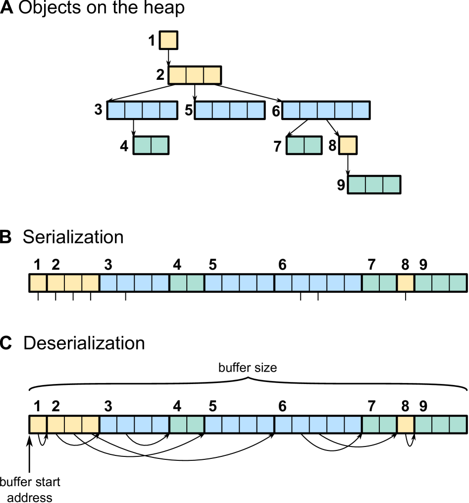
?figurename? 6.2: TeraAgent serialization mechanism

Serialization.

This structure can be serialized by an in-order tree traversal (B). Each tree node (i.e., memory block) is copied to the serialized buffer. Fields inside each memory block that point to other memory blocks are labeled as such, but point to the invalid address $Ox1$. Furthermore, the virtual table pointer of polymorphic classes is replaced by a unique identifier of the most derived class. This step is necessary because we cannot guarantee that the virtual table pointers will be the same on all ranks.

Deserialization.

From the communication subsystem, the deserialization implementation receives a buffer with a starting address, length, and type of the root object. Deserialization consists out of four steps that can be performed in a single traversal of the buffer. First, we traverse the tree from the beginning of the buffer and restore the virtual table pointer for polymorphic objects. The offsets of the memory blocks are determined by their type and retrieved from the compiler. Second, if a pointer is encountered, we set it to the next memory block in the buffer. Third, as we traverse, we count the number of memory blocks, which will be required for memory deallocation (see next paragraph). Fourth, reinterpret the buffer’s starting address as a pointer to the root object and return it to the caller. No other memory reads or writes are taking place. Furthermore, there are no calls to allocate memory besides the single contiguous receive buffer that holds the data.

Mutability.

By returning the root object pointer to the higher-level code, we create the illusion that all contained memory blocks have been allocated separately on the heap. Therefore, higher-level code is not aware that these objects were deserialized using TeraAgent IO and can change them in any way. This includes setting value of attributes, but extends to, for example, adding elements to containers, even if there is not sufficient space in the buffer. In this scenario, the vector implementation notices the capacity is reached, allocates a new memory block on the heap (separately from the buffer) and deallocates the obsolete memory block inside the deserialized buffer.

Deallocation.

As we have seen in the vector example above, higher-level code will at some point try to deallocate memory blocks by calling delete. These delete calls, however, would crash the memory allocator, due to the missing corresponding new call. To maintain the illusion, we intercept all calls to delete and filter those that fall into the memory range of the deserialized buffer. If the number of expected delete calls (determined during deserialization) matches the intercepted delete calls, we deallocate the whole buffer and remove the filter rule.

The disadvantage that memory is leaked if not all memory blocks are freed in a deserialized buffer can be solved for TeraAgent. First, the aura region is completely rebuilt in each iteration, which means that the previous aura information is completely destroyed. Second, for agent migrations and load balancing data, we rely on the periodic agent sorting mechanism in BioDynaMo. Agent sorting changes the memory location of agents to improve the cache hit rate. During this process all agents are copied to a new location and the old ones are deallocated. Figure 6.10 shows that the memory consumption does not increase by using the TeraAgent serialization mechanism.

6.2.3 Data Transfer Minimization

Agent-based modeling is an iterative method. Figure 6.3 shows three successive iterations of the cell clustering simulation. We can observe that the cell position change only gradually between iterations while the cell type and diameter do not change at all. We leverage this observation to reduce the amount of data that must be transferred between MPI ranks to update the aura region by using delta encoding. The implementation of delta encoding is built on top of the TeraAgent serialization mechanism (see Figure 6.4).

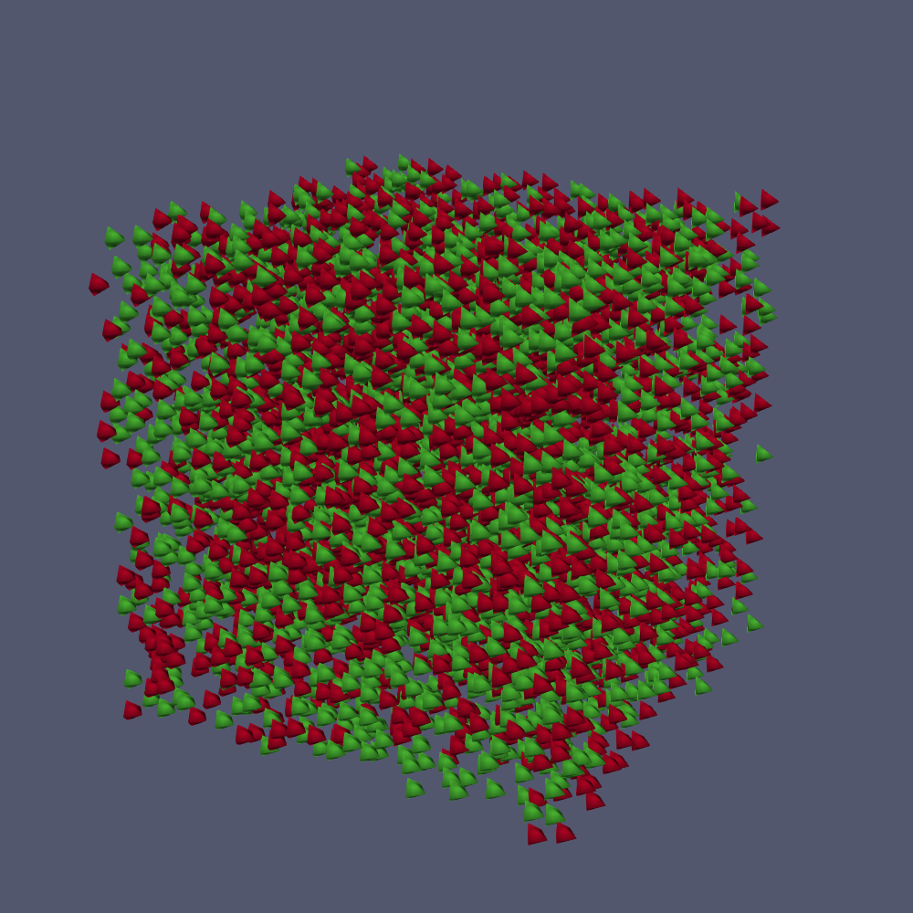
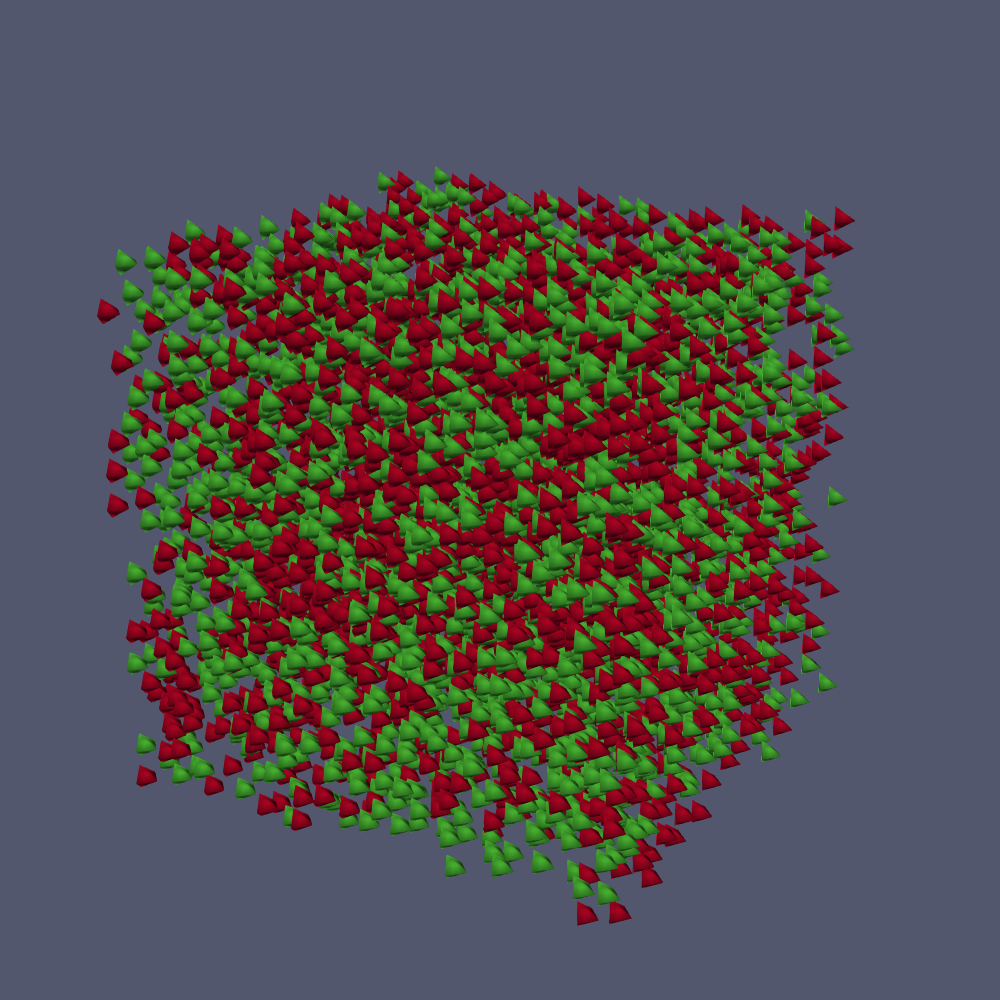
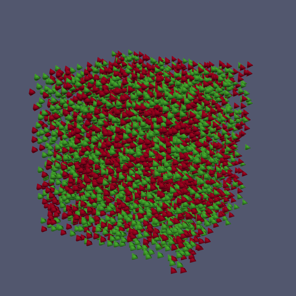
?figurename? 6.3: Cell clustering visualization for the first three iterations

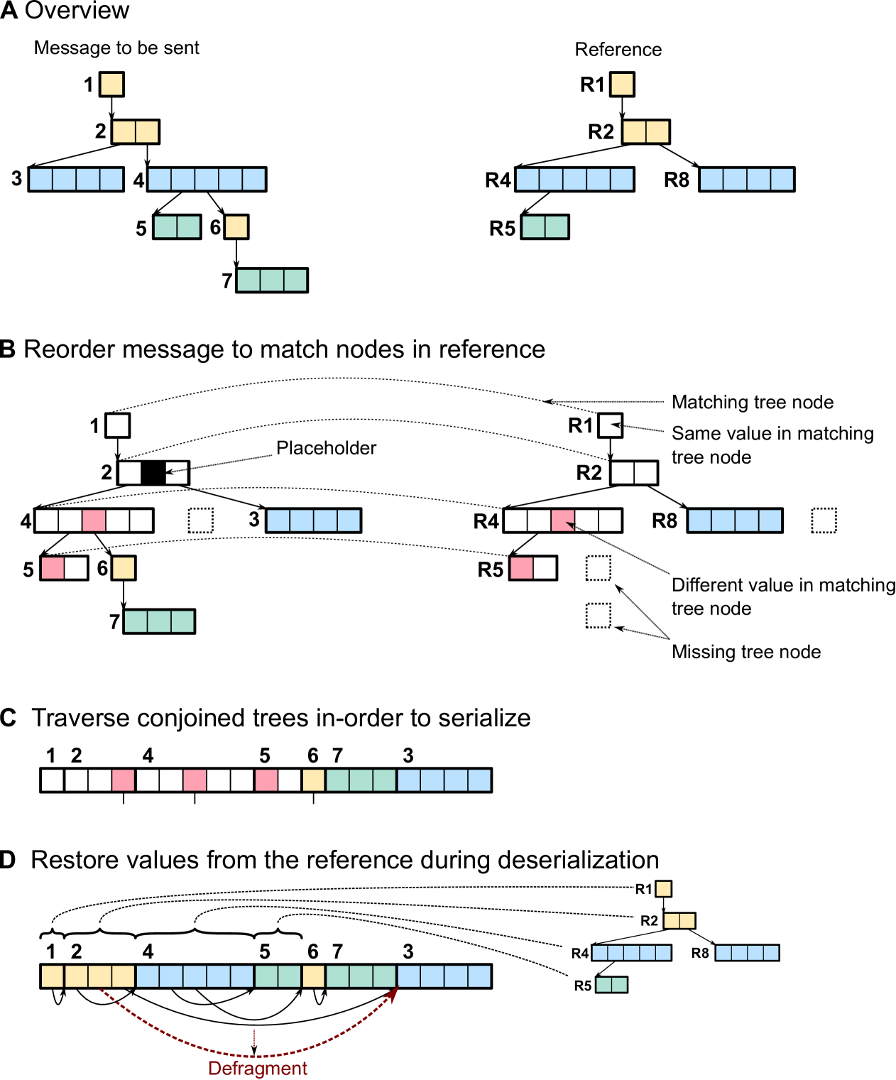
?figurename? 6.4: TeraAgent delta compression

Each sender and receiver pair stores the same reference. The sender calculates the difference between the message and the reference, compresses it and sends it to the receiver. On the receiving side, the process is reversed to restore the original message. The receiver uncompresses the buffer and restores the original message by inverting the difference operation using the received buffer and the stored reference as operands. At regular intervals, sender and receiver update their reference.

More precisely, the sender reorders the message at the agent pointer level (B). Agents which exist both in the message and the reference are moved to the same position that the agent has in the reference. Agents that exist in the reference and not in the message are indicated by an empty placeholder, a value that cannot occur at the same tree depth in the message. In the TeraAgent case, this is simply a null pointer. Lastly, agents that exist in the message and not in the reference are appended at the very end. Reordering agents does not affect the correctness of a TeraAgent simulation.

After the matching stage (B), the TeraAgent serialization mechanism (C) traverses the two conjoined trees, in the same way as described in Section 6.2.2.1. The only difference is that if a match is found in the reference, the difference between the two is written to the result buffer. Since the message is reordered at the sender, we do not need to send additional information about the agent order.

During deserialization (D), we use the data stored in the reference to restore the original message. Lastly, we defragment the message by removing any placeholders that were inserted during the matching stage (B). Note that defragmentation will not restore the original agent ordering as shown in (A). The defragmented message is then passed to higher-level code.

By using this mechanism, TeraAgent reduces the data movement bottleneck and increases the efficiency of distributed execution.

6.2.4 Implementation Details

6.2.4.1 Partitioning Grid

One important data structure in the distributed simulation engine is the partitioning grid, which is responsible for the domain decomposition of the simulation space as shown in Figure 6.1. We use Sierra Toolkit (STK) [436], because it is (i) an established tool maintained as part of Trilinos [437], (ii) well integrated with the load balancing framework Zoltan2 [438], and (iii) has the ability to export the grid in exodus format [439], which our main visualization framework ParaView [392] can read. However, since STK is a generic mesh library, capable of much more than processing rectilinear grids, these functionality comes with a performance penalty in terms of compute and required memory. Furthermore, although STK uses Kokkos [440] for shared memory parallelism, we observe that if TeraAgent is executed in MPI hybrid mode (MPI/OpenMP), most threads are idle during balancing and mesh modification calls into STK. As an alternative, we also considered the parallel grid library [441], but experienced difficulties generating very large grid sizes.

To reduce the memory and compute footprint of STK’s partitioning grid, we introduce a parameter to make the partitioning box length a multiple of the neighbor search grid (see Figure 6.1). The higher this factor is chosen the less memory and compute resources are needed for the space partitioning, but at the cost of increased granularity at which load balancing decisions can be made.

6.2.4.2 Serialization

The TeraAgent IO mechanism (Section 6.2.2.1) requires that (de)serialization methods (also known as TeraAgent IO functions) are available for all types in the message. TeraAgent provides the necessary implementation for its internal classes, the standard template library (STL) classes, and important groups of types (e.g., polymorphic types, pointers, and plain arrays). Due to the design decision to opt for a very lightweight deserialization method, the implementation of the (de)serialization methods depends on its internal attributes (i.e., the concrete implementation), rather than the public interface. This design decision might increase the maintenance effort. However, the TeraAgent IO methods follow a regular structure and can be generated automatically in most of the cases. This is especially true for all user-defined classes in this chapter. Although the (de)serialization methods are currently written by hand, they can easily be integrated into BioDynaMo’s existing code generation stages. BioDynaMo uses code generation during compile time, and during runtime using the C++ just-in-time compiler cling [423].

Custom TeraAgent IO functions are necessary if classes contain pointer attributes, whose memory is not owned. An example could be an array-based stack implementation with an attribute that points to the current top of the stack. To this end, TeraAgent allows for custom implementations of the IO functions that will replace the automatically generated ones.

To intercept delete calls, we overwrite all global C++ delete operators and insert a call to the delete filter, which returns if the delete should be filtered out or executed. This design choice causes some challenges in combination with performance or correctness tools (e.g., valgrind) that use LD_PRELOAD to inject their own implementation of new and delete and prevent the TeraAgent ones from being executed. For valgrind, we solved this issue by patching its code.

6.2.4.3 Communication

For the majority of data transfers, we use non-blocking point to point communication (MPI_Isend, MPI_Irecv, and MPI_Probe). This choice allows for overlapping communication with computation to hide latency. For regular communication patterns that occur between neighbors, we issue speculative receive requests right after the previous transfer finished, to avoid delay through late receivers. If the neighbors of a rank change due to load balancing, obsolete speculative receives are cancelled.

Furthermore, we transmit large messages in smaller batches to reduce the memory needed for transmission buffers, compression, and serialization.

6.2.4.4 Distributed Initialization

Although the distributed simulation engine has the capability to migrate agents to any other MPI rank (Section 6.2.1), we try to avoid a costly mass migration of agents during the initialization stage, by trying to create agents on the authoritative rank. This is straightforward for regular geometric shapes (e.g., agents created on a surface defined by a function), but we also address agent populations that are created using a uniform random number distribution within a specific space. Each rank determines the fraction of the given target space with its authoritative volume, and adjusts the number of agents for this space and the bounds accordingly, if the number of agents for each node is sufficiently high.

6.2.4.5 Load Balancing

Load balancing has two goals. First, partition the simulation space in a way that simulating one iteration takes the same amount of time on all ranks. Second, the partitioning should minimize the distributed overheads, e.g., the number of aura agents that must be exchanged.

TeraAgent provides two classes of load balancing methods to achieve these goals: global and diffusive.

The global balancing method is based on STK and Zoltan2. We provide their functionality for TeraAgent users and choose the recursive coordinate bisection (RCB) algorithm as default. We apply a weight field on the partitioning grid and set the weight of each partitioning box based on the number of agents contained and scale it by the runtime of the last iteration. Zoltan2 now partitions the space in a way that the sum of all owned partition boxes is distributed uniformly between all ranks. This approach might lead to a new partitioning that differs substantially from the previous one, causing mass migrations of agents to their new authoritative rank.

Therefore, we also implement a diffusive approach in which neighboring ranks exchange partition boxes. Ranks whose runtime exceed the local average, send boxes to neighbors that were faster than the local average.

6.2.5 Improvements and Modifications to BioDynaMo

This section describes the necessary modifications and improvements to the existing OpenMP parallelized BioDynaMo version to enable distributed execution.

Parallelization Modes.

By building upon and extending the shared-memory capabilities, we provide two distributed execution modes: MPI hybrid (MPI/OpenMP), and MPI only. For the MPI hybrid mode, we launch one MPI rank for each NUMA domain on a compute node, while for MPI only we launch one rank for each CPU core. On today’s modern hardware with constantly increasing CPU core counts, the MPI hybrid mode can reduce the number of ranks currently by almost two orders of magnitude. We therefore expect the MPI hybrid mode to be more efficient. The MPI only mode, on the other hand, provides benefits when interfacing with third party applications that are only parallelized using MPI. In the MPI hybrid mode, these applications, would leave all but one thread per rank idle.

Switching between parallelization modes does not require recompilation of TeraAgent.

Unique Agent Identifiers.

BioDynaMo uses unique agent identifiers to address agents, since the actual memory location might change due to agent sorting. Agent sorting improves the performance by reordering agents in a way that agents that are close in 3D space are also close in memory (see [171]). The identifier is comprised of two fields: $\langle index,reused\_counter\rangle$ and has the following invariants: At any point in time, there is only one (active) agent in the simulation with the same index. If an agent is removed from the simulation, this index will be reused, but to satisfy uniqueness the reuse_counter is incremented. This design allows the construction of a vector-based unordered map, where the first part of the identifier (the index) is used to index the vector. This map allows for lock-less additions and removals to distinct map elements .

However, this solution does not work without changes for distributed executions with agent migrations and aura updates, because the invariant that the $index$ of the identifiers are almost contiguous does not hold anymore. This would waste a considerable amount of memory in the vector-based unordered map.

Therefore, we rename the existing identifier to “local identifier” and introduce also a global identifier $\langle rank,counter\rangle$. Rank is set to the rank where the agent was created, and “counter” is a strictly increasing number. The global identifier of an agent is constant, but the agent might have various different local identifiers during the whole simulation.

We implement this change minimally invasive. The translation between local and global identifier happens only during serialization if the agent is transferred to another rank, or written to disk as part of a backup or checkpoint. Global identifiers are only generated on demand. If there are no backups or checkpoints and the agent stays on the same rank throughout the simulation, the agent will only have a local identifier.

Incremental Updates to the Neighbor Search Grid (NSG).

Chapter 5 showed that our optimized uniform grid implementation performed best for the benchmarked simulations. Updates to the NSG required a complete rebuild, which was adequate so far. The distributed simulation engine, however, relies on the NSG not only to search for neighbors of an agent, but also to accurately determine the agents in a specific sub volume for agent migrations, aura updates, and load balancing. Rebuilding the complete NSG after each of these steps would be prohibitively expensive. Therefore, we adapted the implementation to allow for incremental changes, i.e., the addition, removal, and position update of single agents.

Modularity Improvements.

Alongside high-performance, modularity is another key design aspect of TeraAgent. We have therefore made additional efforts in this direction during the development of TeraAgent and made three main changes. First, we introduce the VisualizationProvider interface to facilitate rendering of additional information besides agents and scalar/vector fields. We use an implementation of this interface to render the partitioning grid as can be seen in Figures 6.5. Second, we add the SimulationSpace interface to explicitly gather information about whole and local simulation space in one place. Third, we refactor the code and introduce the SpaceBoundaryCondition interface and refactor the implementations for “open”, “closed”, and “toroidal”.

6.3 Evaluation

6.3.1 Benchmark Simulations

We use four simulations from [171, 188] to evaluate the performance of the simulation engine: cell clustering, cell proliferation, and use cases in the domains of epidemiology, and oncology. We did not include the neuroscience use case, since it requires the ability to modify neighbors, which is currently not implemented yet and chose only one of the two cell clustering implementations. Table 1 in [171] shows that these simulations cover a broad spectrum of performance-related simulation characteristics.

6.3.2 Experimental Setup and Reproducibility

All tests were executed in a Singularity container with an Ubuntu 22.04 based image. We used two systems to evaluate the distributed simulation engine. First, we used the Dutch national supercomputer Snellius (genoa partition) where each node has two AMD Genoa 9654 processors with 96 physical CPU cores each, 384 GB total memory per node, and Infiniband interconnect (200 Gbps within a rack, 100 Gbps outside the rack) [442]. Second, we use a two node system (System B) where each node has four Intel Xeon E7-8890 v3 CPUs processors each with 72 physical CPU core, 504 and 1024 GB main memory, and Gigabit Ethernet interconnect. We are therefore able to evaluate the performance with a commodity and high-end interconnect.

We use the term “simulation runtime” for the wall-clock time needed to simulate a number of iterations, which excludes the initialization step and tear down.

We will provide all code, the self-contained Singularity image, more detailed information on the hardware and software setup, and instructions to execute the benchmarks upon publication on Zenodo.

6.3.3 Correctness

To ensure the correctness of the distributed simulation engine, we added 180 automated tests, and replicate the results from [188, 171]. Figure 6.5 shows the quantitative comparison of the simulation compared to analytical (epidemiology use case) or experimental data (oncology use case), and a qualitative comparison for the cell sorting simulation. We can observe that TeraAgent produces the same results as BioDynaMo.

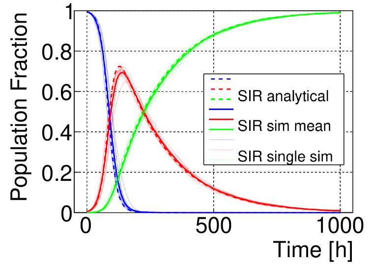
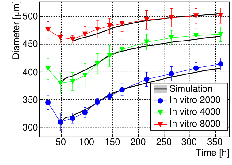
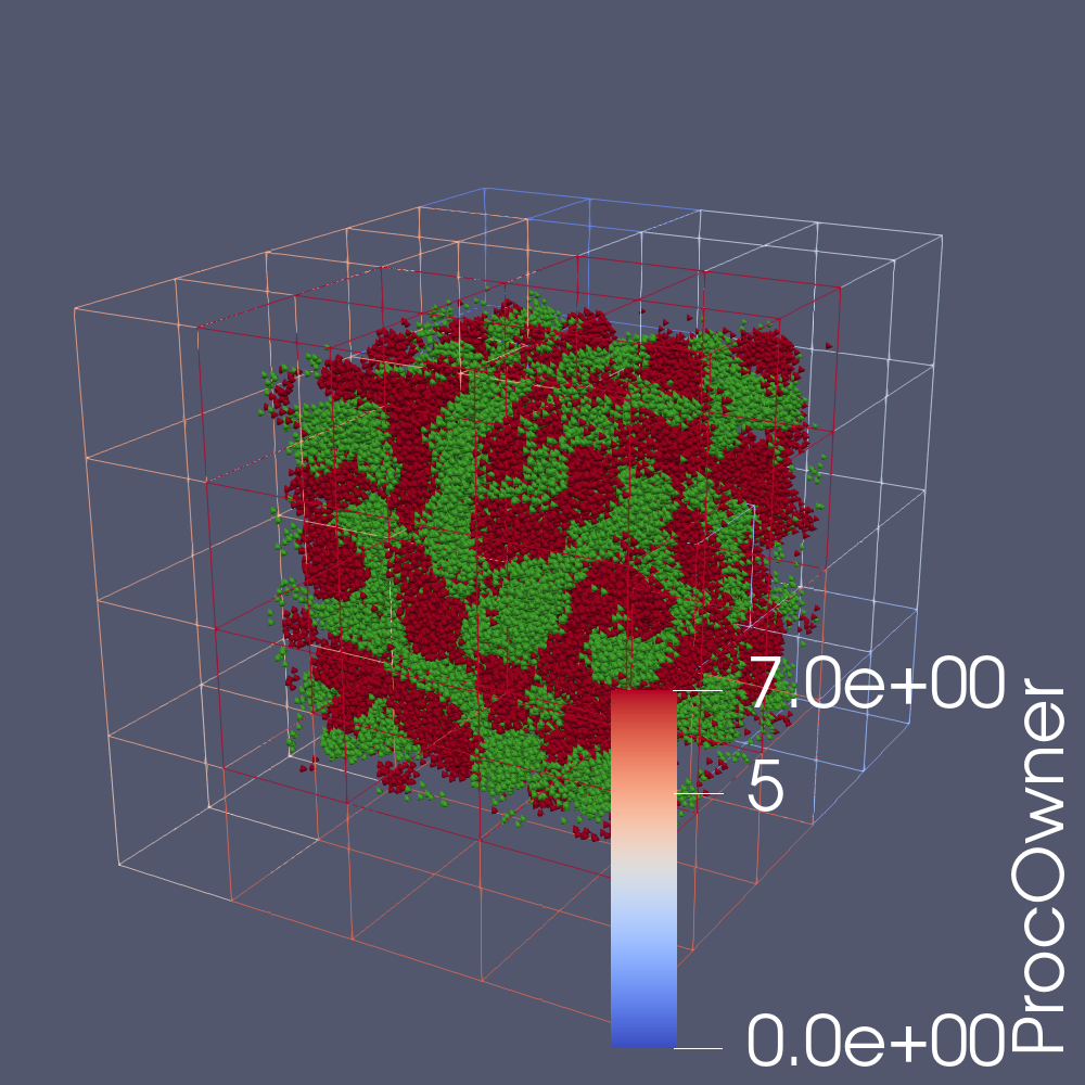
?figurename? 6.5: Result verification of TeraAgent

6.3.4 Seamless Transition From a Laptop to a Supercomputer

User-friendliness is a key design aspect, alongside our focus on performance. Regarding distributed computing, the model definitions for the four benchmark simulations are completely transparent to the user. Only the evaluations for the epidemiology and oncology use cases require additional code for distributed execution.

The changes in the epidemiology simulation, are limited to two lines of code. To create the graph shown in Figure 6.5, the engine has to count the number of agents for the three groups (susceptible, infected, and recovered). For distributed executions the rank local results have to be summed up to obtain the correct result. To do that, we provide the function SumOverAllRanks, which hides the MPI related function call. Furthermore, to save the generated plot to disk, we have to make sure that only one rank writes to the same file location. This goal can be achieved by telling the other ranks to exit the function before the save function is executed. We can achieve this with the preprocessor macro IF_NOT_RANK0_RETURN.

Also the tumor spheroid simulation requires extra code to generate the result plot (Figure 6.5). To accurately measure the tumor diameter in the simulation, we determine the volume of the convex hull, from which we can calculate the diameter by assuming a spherical shape. Chapter 5 uses libqhull [443], a library which is not distributed. Consequently, the simulation contains a couple lines of extra code to transmit agent positions to the master rank to perform the diameter calculation. For simulations with a larger number of agents, we use a more approximate method, by determining the enclosing bounding box. The approximate method is provided by TeraAgent and is the same whether executed distributed or not.

To summarize, for many simulations our users do not need to know about distributed computing to scale out a simulation to tens of thousands of CPU cores, as demonstrated in this chapter. Researchers can start the development on a laptop and seamlessly transition to more powerful hardware as the model size and complexity grows.

6.3.5 Comparison with BioDynaMo

We compare the performance of TeraAgent in MPI hybrid and MPI only mode with BioDynaMo. The benchmarks were executed on one node of System B with $10^{7}$ agents and for all iterations of the simulations. Figure 6.6 shows that MPI hybrid mode performs close to the OpenMP version (slowdown between 4–9%) despite the extra steps required in distributed execution (Figure 6.1). The performance drops significantly for MPI only (slowdown between 26–34%), which uses 18$\times$ more MPI ranks and also does not use hyperthreading.

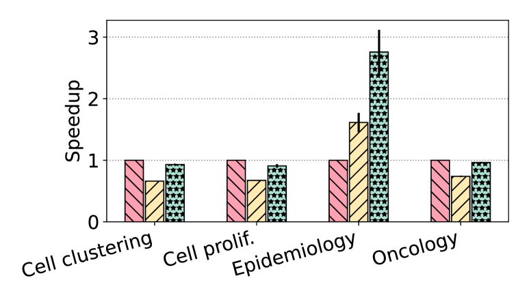
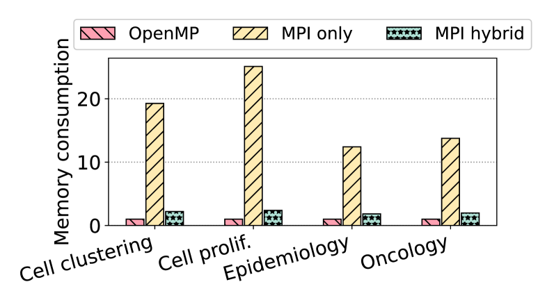
?figurename? 6.6: Speedup (left) and normalized memory consumption (right) of TeraAgent in MPI only and MPI hybrid configuration with respect to BioDynaMo (OpenMP).

For the epidemiology simulation, both distributed modes outperform (speedup of MPI hybrid: 2.8$\times$) BioDynaMo. Chapter 5 shows that the performance of the epidemiology simulation is sensitive to the memory layout. Although, BioDynaMo is NUMA-aware, not all data structures (e.g., the neighbor search grid) are separated for each NUMA domain. We attribute the observed performance increase to reduced cross-CPU traffic of the distributed engine, which outweighs the overheads of aura updates and agent migrations.

The memory consumption increases approximately by $2\times$ for the MPI hybrid mode due to the additional data structures. A large part of the memory required by the MPI only mode can be attributed to the use of cling [423]. In the current implementation, each rank has its own instance of cling, which requires several hundred MB of memory on its own.

6.3.6 Improved Interoperability

This section demonstrates how the distributed simulation engine improves interoperability with third party software by enabling the interaction from the performance aspect. A well-suited example to demonstrate this improvement is ParaView, the main visualization provider of BioDynaMo. ParaView offers two visualization modes: export mode in which the simulation state is exported to file during the simulation and visualized afterwards, and the situ mode in which ParaView accesses the agent attributes directly in memory and generates the visualization while the simulation is running.

Although ParaView uses distributed and shared-memory parallelism, the scalability of using threads alone is very limited (see Figure 6.7). Therefore, BioDynaMo used mainly the export mode. TeraAgent, however, is now able to leverage the unused potential of in situ visualization.

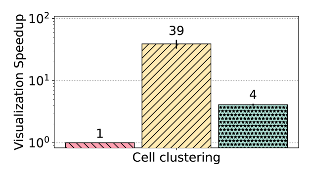
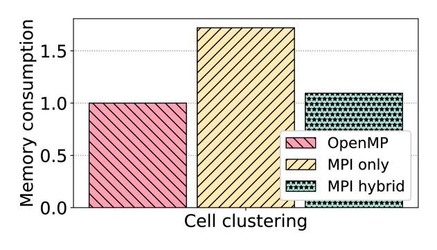
?figurename? 6.7: Performance comparison of in situ visualization with ParaView on System B comparing TeraAgent in MPI only and MPI hybrid configuration with BioDynaMo (OpenMP).

On one System B node, we execute the cell clustering simulation with 10 million agents for 10 iterations (Figure 6.7). Each iteration renders one image. We evaluate three configurations: BioDynaMo using OpenMP (i.e., one rank and 144 threads), and two TeraAgent configurations: MPI only (i.e., 72 ranks with one thread each) and MPI hybrid (i.e., 4 ranks and 36 threads each).

We can clearly see that ParaView’s in situ mode scales mainly with the number of ranks. TeraAgent’s MPI only configuration visualizes 39$\times$ faster than BioDynaMo although it is only using half the number of threads. The memory consumption is dominated by ParaView and therefore shows a less pronounced difference between MPI hybrid and MPI only mode.

6.3.7 Scalability

We analyze the scalability of the distributed engine under a strong and weak scaling benchmark. First, for the strong scaling analysis, we examine how much we can reduce the runtime of a simulation with a fixed problem size by adding more compute nodes. We chose the simulation size such that it fills one server and run it for 10 iterations with node counts ranging from one to 16 (3072 CPU cores) increased by powers of two. Figure 6.8 shows good scaling until 8 nodes (1536 CPU cores), which slows down due to load imbalances and the associated wait times for the slowest rank.

Second, we investigate the performance of the distributed engine by simulating larger models with proportionally increased compute resources. We use $10^{8}$ agents per node and increase the node count from one to 128, which corresponds to 24’576 CPU cores. Figure 6.9 shows that after an initial increase in runtime, a plateau is reached.

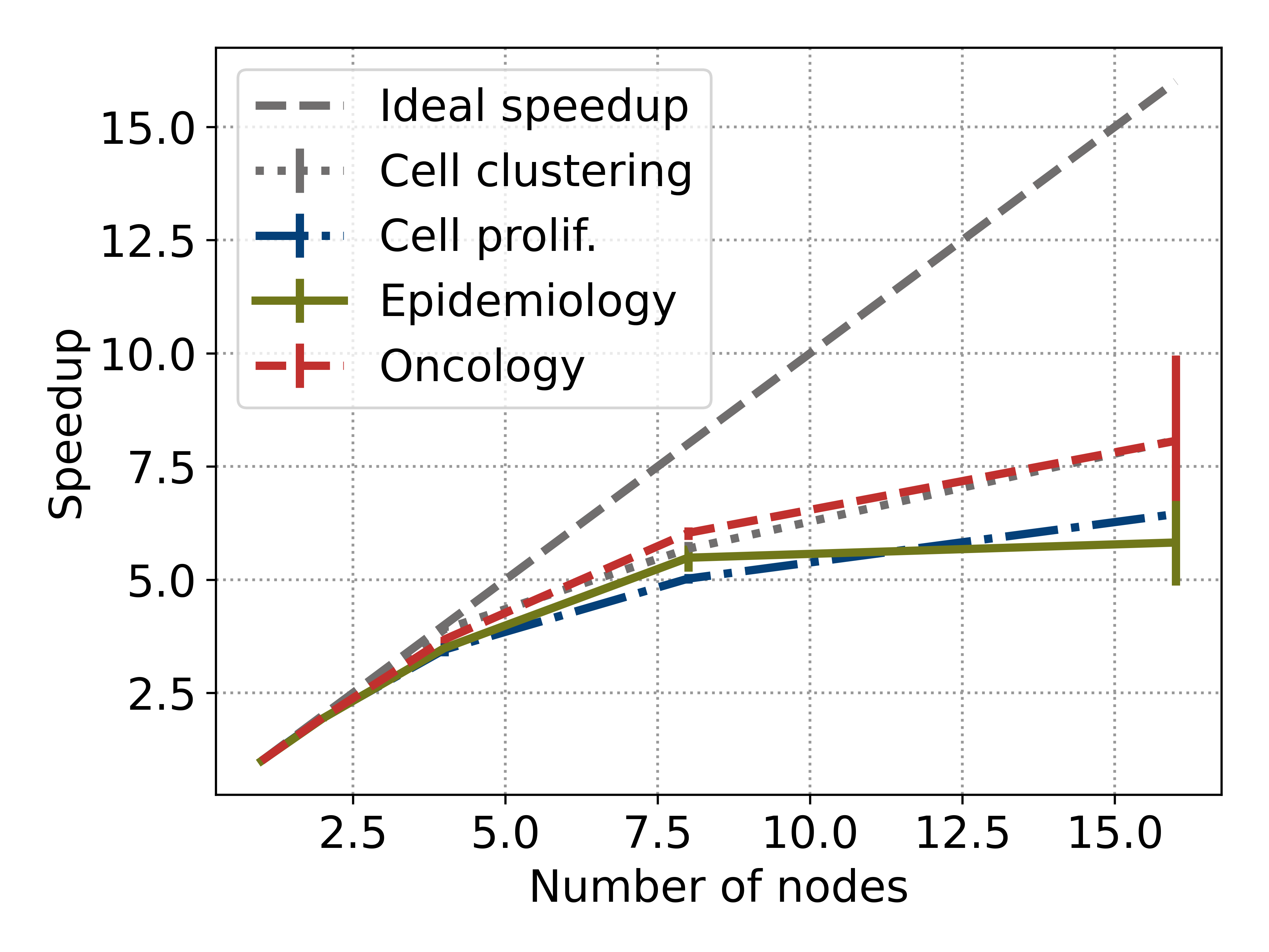
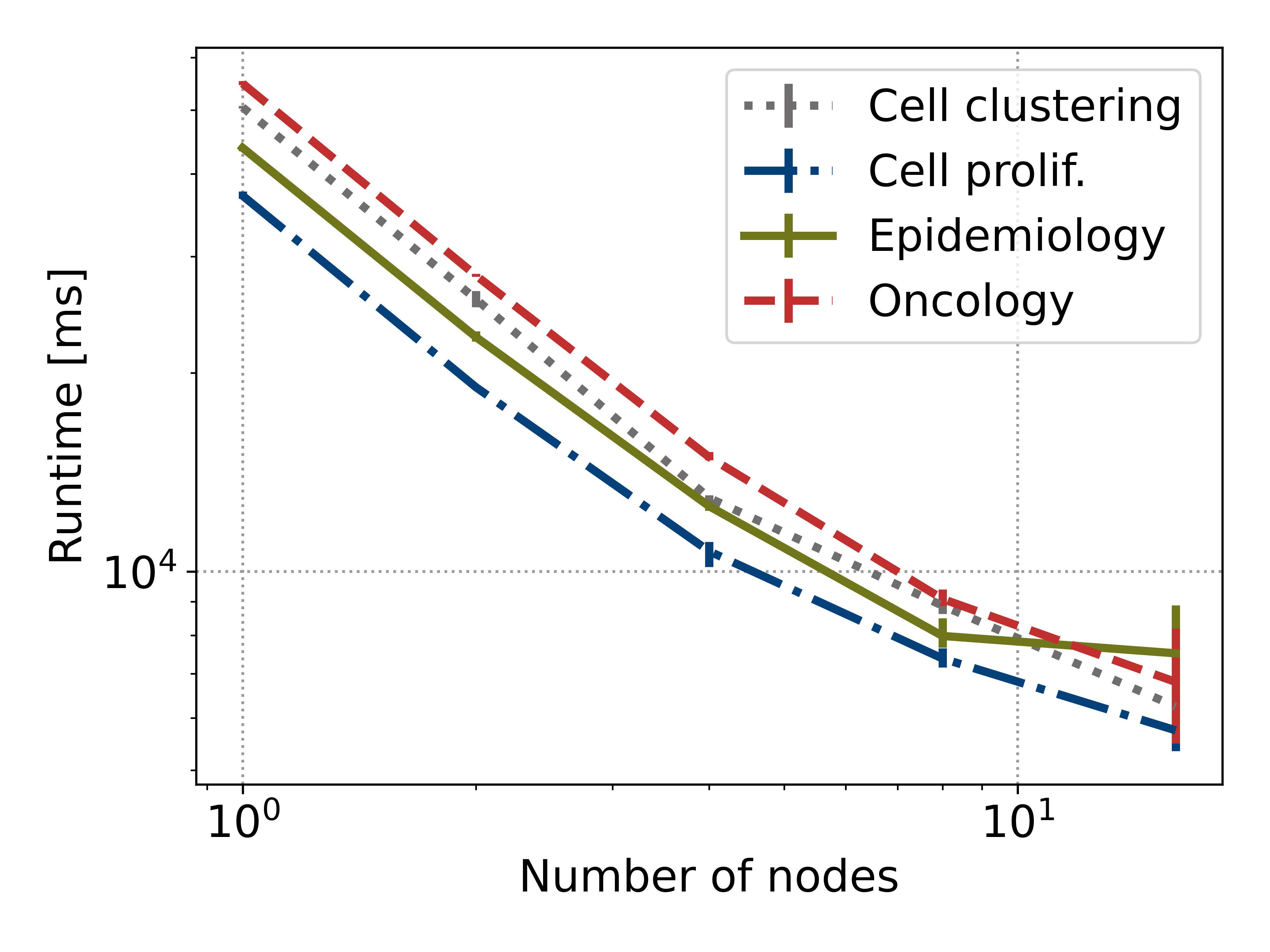
?figurename? 6.8: Strong scaling analysis: speedup with respect to an execution on a single node (left), absolute runtime (right).

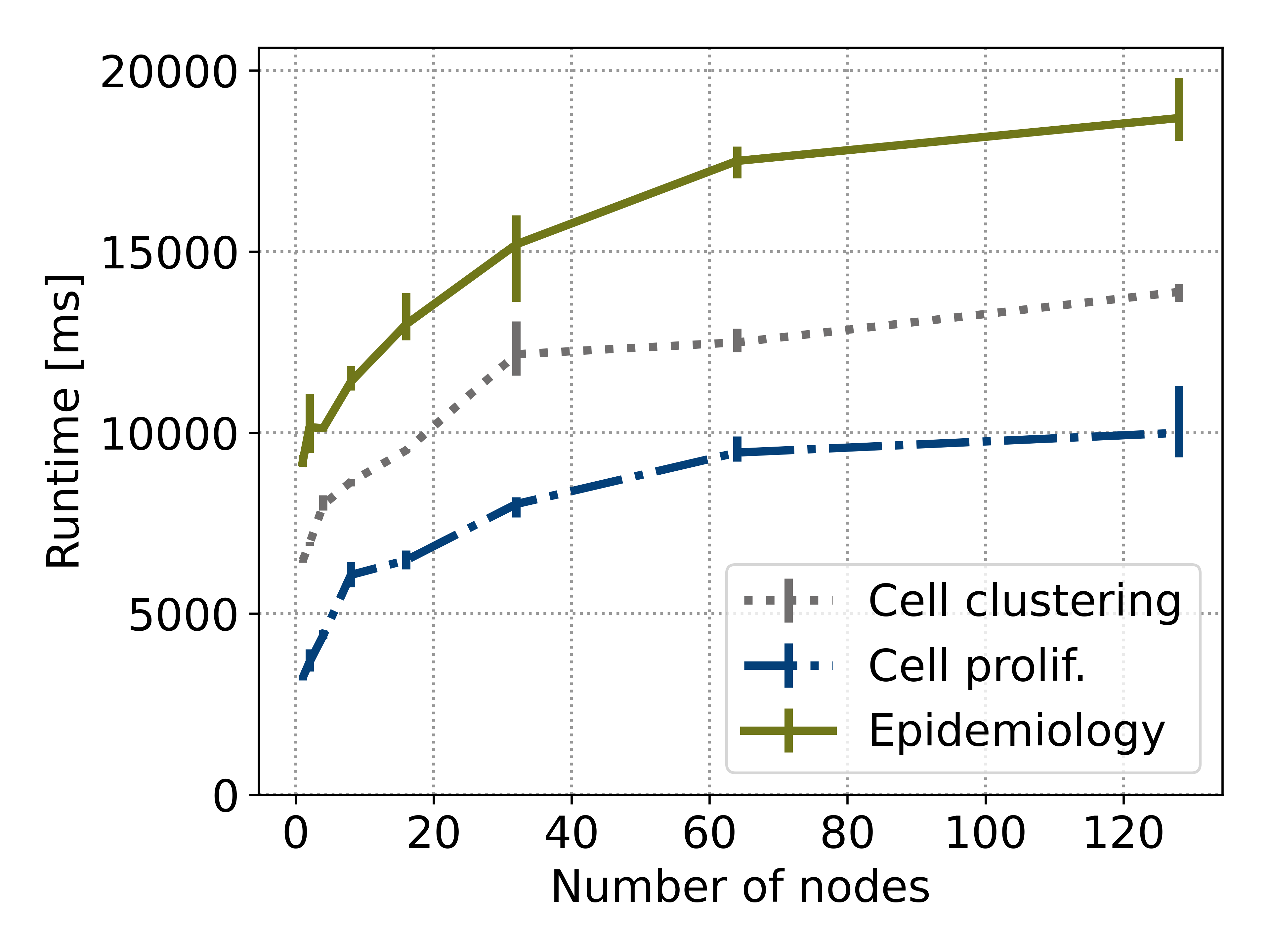
?figurename? 6.9: Weak scaling analysis

6.3.8 Comparison with Biocellion

To compare the performance of the distributed simulation engine with Biocellion [7], we replicate the benchmark from [171]. We execute the cell clustering simulation with 1.72 billion cells on System B. In contrast to [171], we use two nodes due to the additional required memory. We measure a runtime of 15.8s averaged over all iterations using 144 physical CPU cores. This results in $7.56e5$ $\frac{agent\_updates}{s\times CPU\_core}$. As [171], we use the result from the Biocellion paper, because the software is not available under an open source license. Kang et al. report 4.46s per iteration on 4096 CPU cores (AMD Opteron 6271 Interlago), resulting in $9.42e4$ $\frac{agent\_updates}{s\times CPU\_core}$. We therefore conclude that TeraAgent is 8$\times$ more efficient than Biocellion.

6.3.9 Extreme-Scale Simulation

To demonstrate that TeraAgent can substantially increase the state-of-the-art in terms of how many agents can be simulated, we perform two experiments.

First, we execute the cell clustering simulation with 102.4 billion cells (or agents) for 10 iterations. The simulation was executed on 24’576 CPU cores on 128 Snellius nodes using 40 TB of memory and taking on average $7.08\text{\,}\mathrm{s}$ per iteration.

Second, we increase the number of agents even further to 501.51 billion and use 438 nodes with 84’096 CPU cores. To fit this amount of agents into the available main memory, we reduce the engine’s memory consumption by disabling all optimizations that require extra memory, use single-precision floating point numbers, reduce the agent’s size by changing the base class, and reduce the memory consumption of the neighbor search grid. These adjustments reduce the memory consumption to 92 TB, but also increase the average runtime per iteration to $147\text{\,}\mathrm{s}$.

6.3.10 Serialization

This section compares the tailor-made TeraAgent serialization mechanism for the agent-based use case presented in Section 6.2.2 with the baseline ROOT IO (see Figure 6.10). We execute the benchmark simulations on four Snellius nodes in MPI hybrid mode with $10^{8}$ agents for 10 iterations.

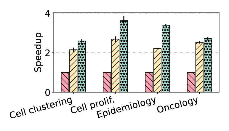
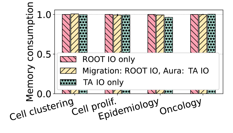
(a) Simulation runtime (left), memory consumption normalized (right)

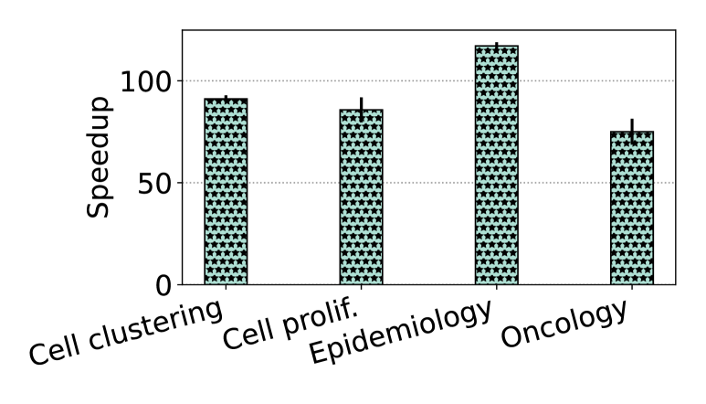
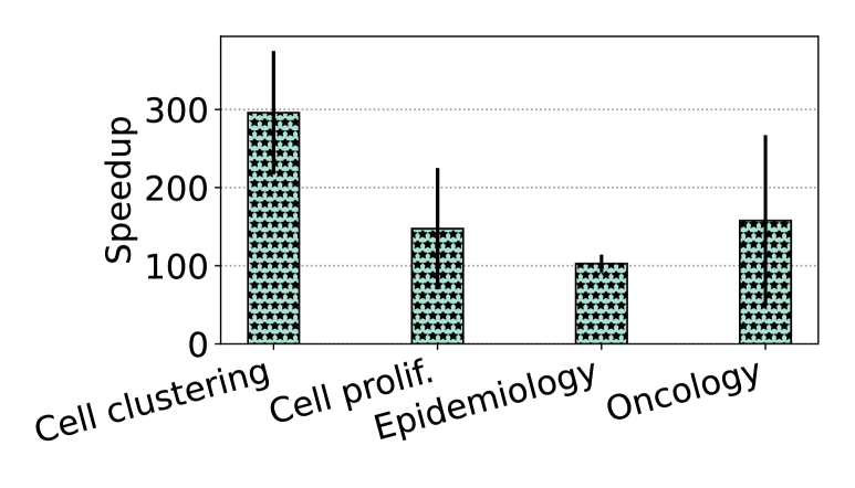
(b) Serialization: aura (left), migrations (right)

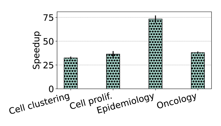
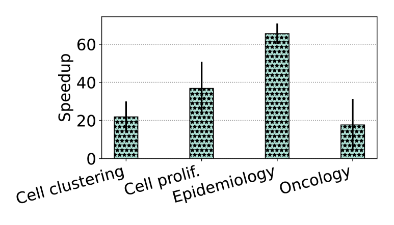
(c) Deserialization: aura (left), migrations (right)

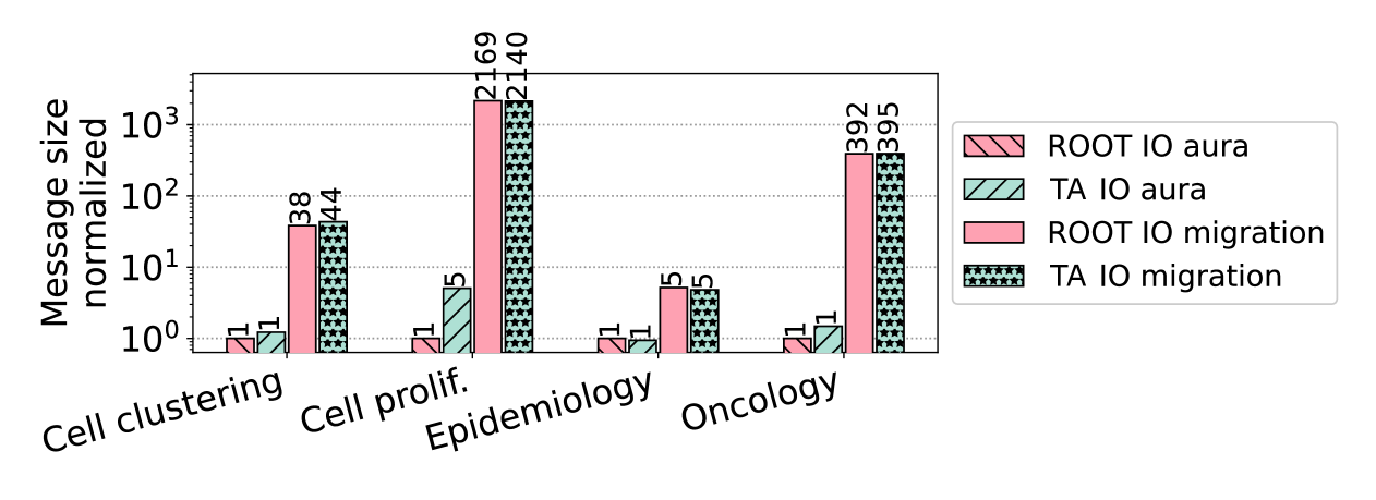
(d) Message size normalized

?figurename? 6.10: Comparison of the TeraAgent serialization mechanism (TA IO) and ROOT IO on Snellius.

Figure 6.10 shows that simulation runtime was reduced by up to 3.6$\times$, while keeping the memory consumption constant. TeraAgent IO serializes the agents up to 296$\times$ faster (median 110$\times$) and also significantly improves the deserialization performance: maximum observed speedup of 73$\times$ (median 37$\times$). Figure 6.10(d) shows that the resulting message sizes are equivalent. The only outlier in cell proliferation is due to the small message size and does not impact the performance negatively.

6.3.11 Data Transfer Minimization

To evaluate the performance improvements of LZ4 compression [444] and delta encoding, we execute all benchmark simulations with $10^{8}$ agents on two System B and four Snellius nodes for 10 iterations. Figure 6.11 shows the comparison on Snellius with TeraAgent IO as baseline. The message size is reduced between 3.0–5.2$\times$ by LZ4 compression and by another 1.1–3.5$\times$ for adding the delta encoding scheme described in Section 6.2.3. This improvement speeds up the distribution operation, which subsumes aura updates and agent migrations, up to 11$\times$. However, the significant speedups of delta encoding do not translate to the whole simulation. The reason is shown in Figure 6.11(b) (right). Delta encoding reduces the performance of agent operations (i.e., the main functionality of the model), caused by agent reordering. The memory consumption is increased slightly for delta encoding enabled by the data structures that holds the reference (median: 3%).

On Snellius, simulation runtime is reduced in three out of four simulations by using LZ4 compression (median improvement: 1.8%). However, due to Snellius’ low latency and high bandwidth interconnect, delta encoding does not lead to further runtime reductions, because the overheads outweigh the benefits.

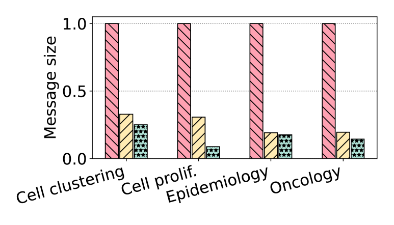
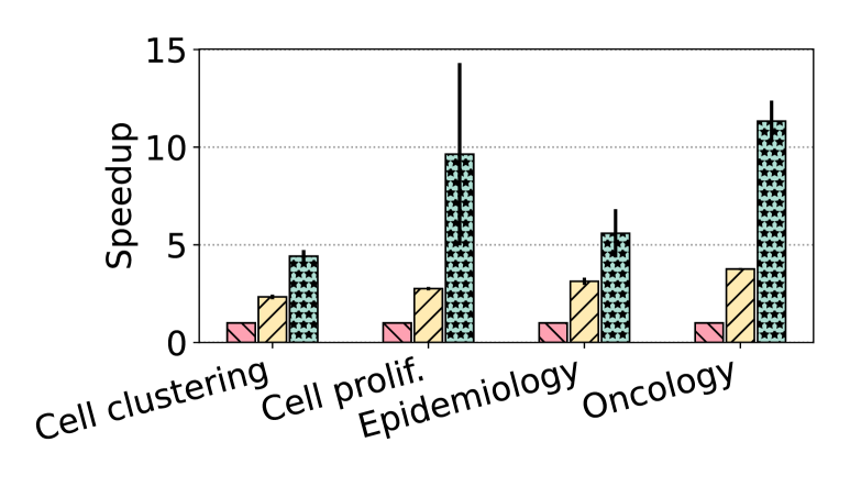
(a) Normalized message size (left) and distribution operation speedup (right)

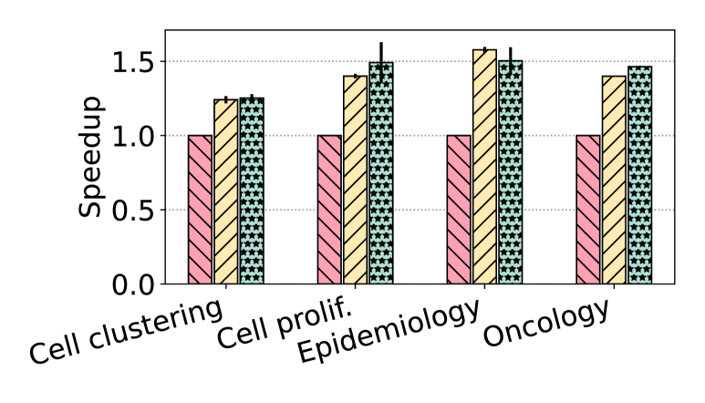
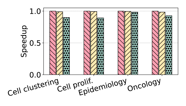
(b) Simulation runtime speedup (left) and agent operations speedup (right)

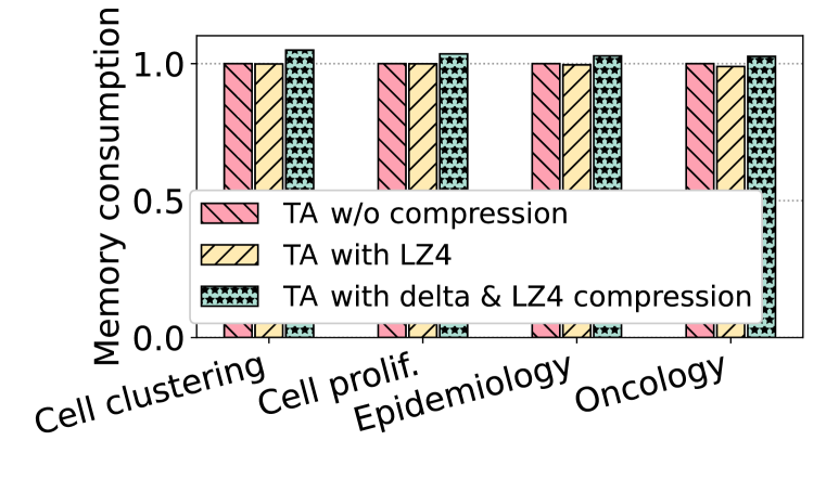
(c) Normalized memory consumption

?figurename? 6.11: Comparison of the TeraAgent IO serialization mechanism with and without compression enabled.

6.4 Conclusion and Future Work

This chapter presents TeraAgent a distributed simulation engine which addresses the scaling limitations of the state-of-the-art agent based simulation platform, BioDynaMo. To do so, our distributed simulation engine 1) enables extreme-scale simulations with half a trillion agents, 2) reduces time-to-result by adding additional compute nodes, 3) improves interoperability with third-party tools from the performance side, and 4) gives users more hardware flexibility. Our distributed simulation engine allows researchers to seamlessly scale out their execution environment from laptops and workstations to clouds and supercomputers. We demonstrate (Section 6.3.4) that such scale-out does not require any model code changes. These results clearly show the benefits of distributed computing capabilities. Researchers can leverage these performance improvements and gain new insights into complex systems by building models on an unprecedented scale that has not been possible before.

?chaptername? 7 Conclusion & Future Work

In summary, this dissertation demonstrates that creating a high-performance, scalable, and modular agent-based simulation platform from the ground up can lead to a drastic reduction in simulation runtime. This reduction enables the execution of larger and more complex simulations, facilitates faster iterative development, and allows for more extensive parameter exploration. This dissertation also demonstrates that a modular platform can significantly enhance adoption across various domains. These major findings come as a result of the dissertation’s three main contributions, which involve the design, implementation, analysis, and optimization of a novel extreme-scale agent-based simulation platform.

Contribution 1: We design, implement, test, and validate BioDynaMo. This process involves defining abstraction layers, developing infrastructure, and setting up a rigorous testing framework. We create a modular design with 1) hidden low-level features so users can focus on the bigger picture without worrying about implementation details, 2) high-level features that provide critical agent-based functionality across various domains, and 3) model building blocks containing domain-specific functions. BioDynaMo’s features are extensively tested with over 600 automated unit, system, and integration tests executed for each change to BioDynaMo’s code repository. We demonstrate BioDynaMo’s capabilities with three simple yet representative use cases in neuroscience, oncology, and epidemiology. We validate these models and BioDynaMo with experimental data and an analytical solution. We show that BioDynaMo’s functionality and flexibility lead to succinct model definitions ranging from 128 to 181 lines of C++ code for the three presented use cases.

Contribution 2: We build a highly efficient multithreaded simulation engine for the BioDynaMo platform. Based on a detailed performance analysis of BioDynaMo, we identify three major areas for improvement and provide solutions to improve BioDynaMo in these three areas. 1) To maximize the parallel part of the simulation, we develop an optimized grid for neighbor searches and parallelize the merging of thread-local results and visualization. 2) Agents often follow computationally inexpensive behaviors, which leads to a memory-bound workload on today’s state-of-the-art CPU hardware. We optimize the memory access pattern and data layout to mitigate this performance issue. We (i) reduce memory accesses to remote DRAM regions (on systems with non-uniform memory architecture) that have higher access latency, (ii) increase the cache-hit rate by bringing agents and their local environment closer together in memory, and (iii) add a faster memory allocator. 3) Based on the observation that some simulations contain regions where agents do not move, we skip the expensive pair-wise force calculation under specific conditions. The results show that our improved single-node BioDynaMo simulation engine is not only highly scalable (with a parallel efficiency of 91.7%) but also efficient in terms of absolute runtime. A single-thread comparison between the improved BioDynaMo and Cortex3D and NetLogo shows a 23$\times$ and 27$\times$ speedup with BioDynaMo. By running BioDynaMo on all 72 CPU cores on our benchmark hardware, while Cortex3D and NetLogo use only one core, we can achieve a speedup of three orders of magnitude. When compared to Biocellion using a simulation with 1.72 billion cells, BioDynaMo accomplishes the same wall-clock runtime but with 9$\times$ fewer CPU cores.

Contribution 3: We further extend the capabilities of BioDynaMo by introducing TeraAgent, a distributed simulation engine that executes one simulation on multiple servers. This capability allows for even larger and more complex simulations, improves interoperability with third-party software, and gives users more flexibility regarding what type of hardware they want to run their simulations on. We identify agent serialization as the main bottleneck and develop a tailored serialization mechanism that reduces unnecessary overheads like checks for object duplication, schema evolution, and unpacking during deserialization. We extend this mechanism with delta encoding to reduce data transfers between processes, which improves performance on systems with commodity interconnect. We demonstrate that the TeraAgent distributed simulation engine can simulate extreme-scale simulations with half a trillion agents using 84’096 CPU cores. Our optimizations reduce the time spent on serialization by 110$\times$ (median) and time spent on deserialization by 37$\times$. Delta encoding reduces the amount of data transferred between servers between 1.1–3.5$\times$. The TeraAgent distributed simulation engine also improves interoperability with third-party libraries that are predominantly parallelized with MPI. Thus the parallel speedup of these libraries depends on the number of processes. Since BioDynaMo executes simulations with one process only, these libraries often utilize only one CPU core. TeraAgent addresses this issue by providing an execution mode that creates one process per CPU core. We demonstrate TeraAgent’s improved interoperability with our visualization library ParaView for the cell clustering benchmark and observe a 39$\times$ visualization speedup of TeraAgent over BioDynaMo.

In conclusion, BioDynaMo and especially TeraAgent set new standards for agent-based simulation platforms by combining high performance, scalability, modularity and user-friendliness. TeraAgent is the first agent-based simulation platform that supports more than half a trillion agents.

7.1 Future Work

We identify multiple opportunities for future work that can extend the library of model building blocks, make BioDynaMo/TeraAgent accessible to a wider community, build a vibrant community, achieve bit-reproducible simulation results, add support for implicit differential equation solvers, extend GPU support, automated performance parameter tuning, and taking advantage of processing in memory systems.

7.1.1 Extending the Library of Model Building Blocks and Demos

The time required to implement a model in BioDynaMo significantly depends on 1) whether the required model building blocks (Section 4.5), e.g., agents, behaviors, the environment, and other functionality, are readily available, and 2) if these building blocks can be easily understood through documentation and their use in well-explained demos and tutorials (see for example Appendix E). Our initial approach to motivating users to spend extra time generalizing their functionality and contributing it back has had limited success. Therefore, an organized approach to extending the library of model building blocks is needed to increase the adoption of BioDynaMo. We believe there are at least two directions.

First, although BioDynaMo provides building blocks for its core domains (e.g., neuroscience, cancer research, and epidemiology), their number needs to be extended to further strengthen BioDynaMo’s position. The following additions would be valuable: 1) the ability to simulate the electrophysiology of neurons [445, 446, 447, 448, 449], 2) support for more agent shapes besides spheres and cylinders, 3) and map-based environments for epidemiological models [88, 110, 111].

Secondly, BioDynaMo should expand to other areas that may require a large number of agents and which would, therefore, greatly benefit from BioDynaMo’s performance characteristics. Immunological models would benefit from having cell definitions for macrophages, T- and B-lymphocytes and their subtypes, memory cells, antibodies, and more [62, 63, 64, 65, 66, 67, 68, 69, 70, 71]. In finance and economics, users may need a virtual stock exchange component for financial market models, agents that can behave irrationally, agents who learn, and a social network of agents that influence their behavior [122, 123].

7.1.2 Making BioDynaMo Accessible to a Wider Community

We have observed that simulation definitions in C++ challenge computational researchers with a more Matlab- or R-based background. Although we have put substantial effort into making BioDynaMo easy to use, choosing the C++ programming language is a limiting factor. C++ is an excellent choice for performance-oriented software but is more challenging to learn than, for example, Python. Future research focusing on alternative ways to define a model could make the BioDynaMo platform more appealing to a broader audience, while hopefully keeping the same performance and efficiency of the platform.

A promising key idea for this work is to enable users to define their model in higher level languages like Python. ROOT, for example, uses dynamic Python bindings [450] and lets physicists define their data analysis in Python code. Python bindings present a promising solution to assemble a simulation from an extensive model library (Figure 4.24). At present, however, most BioDynaMo models necessitate user-defined agents, behaviors, or operations. When user-defined classes are written in a higher level language, a key challenge is the performance overhead that arises from frequent crossings of the language boundaries. This issue can be observed between Java and C++ in [451]. The performance challenge of language interaction is not specific to agent-based simulation. Recent work by Kundu et al. [452] addresses this issue by making JIT-compiled Python (using Numba [453]) available to C++.

Kundu et al.’s work could be a starting point for BioDynaMo to be even easier to use. Advanced Python integration would simplify simulation development and allow users to access Python’s vast library ecosystem, while ideally keeping the performance and scalability of BioDynaMo.

7.1.3 Community Building

This dissertation presents an agent-based simulation platform with performance capabilities exceeding state-of-the-art competitors by a large margin. Despite these capabilities and successful use cases [10, 8, 23, 11, 24, 25, 41, 87, 9, 18, 17, 185, 13, 183, 184, 182], a larger developer and user base is needed to unfold the project’s innate potential.

Without an active and vibrant development community, any open-source project fears stagnation and decline. Therefore, a larger development community is required to keep the project alive and thriving through timely user support, active maintenance, frequent releases, and further feature development to consolidate BioDynaMo’s position in simulation fields like computational biology, while expanding into new areas where BioDynaMo could make a difference.

An active development community that follows these guidelines builds the required trust with new users to invest their time and resources to base their models on the BioDynaMo platform. On the other hand, a growing number of users provide essential feedback and direction for further improvements in the code base, motivate the developers, and, last but not least, legitimate the investments made into the project.

However, attracting, onboarding, and retaining talent is a challenging endeavor. There is no shortage of other open-source projects. According to Github, the largest open-source code platform, over 300 million code repositories compete for approximately 120 million registered developers on the platform [454].

To differentiate in this crowded marketplace and attract the necessary talent, a project needs to be convincing on several dimensions described in the literature. These works highlight the importance of managing the first impression, providing fast feedback, welcoming community, extensive documentation, transparent processes, and many other sometimes subtle hints that make a difference [455, 456, 457, 458, 459, 460].

Riehle also points out that: “[e]conomically rational developers strive to become committers to high-profile open source projects to further their careers …” [457]. Therefore, the project should follow the SAFARI Research Group’s motto of “Thinking Big and Aiming High” [461, 462] to achieve high-impact results, which will also help to increase the project’s visibility and capability to attract new highly-motivated and capable members.

7.1.4 Achieving Bit-Reproducible Simulation Results

Currently, only two execution modes (Figure 4.5) produce deterministic simulation results. First, serial executions , and second, distributed executions without dynamic load balancing where each rank is limited to one thread (MPI only mode). All the other parallel modes are non-deterministic but produce statistically reproducible results. Non-determinism impedes debugging and testing and causes unstable gradients during parameter optimizations.

The most significant source of non-determinism is different random number sequences an agent observes. BioDynaMo has thread-private random number generators. A different execution order will lead to different random numbers during the agent update. A potential solution can happen in four steps. First, we can create a pseudo-random number generator (PRNG) for each agent that is only used during its update. Counter-based PRNGs [463] could be a good choice and address the large state size of, e.g., Mersenne Twister [464]. Second, we can replace the InPlaceExecutionContext, with the CopyExecutionContext (Section 5.2.1). The latter execution context commits all changes at the end of the simulation, providing a consistent view of the neighbor’s attributes independent of the order in which agents are updated. However, this comes at higher memory size and performance penalties, as shown in Section 5.6.14. Third, simulation initialization must be ensured to be deterministic. Fourth, further attention must be given to other non-associative reductions and transcendental functions [465]. In summary, addressing the sources of randomness improves debugging and testing and leads to stable gradients for parameter optimization.

7.1.5 Adding Support for Implicit Differential Equation Solvers

Many agent-based models (e.g., tissue models) incorporate a continuum-based component to simulate processes such as substance diffusion [10], heat dissipation [183, 184], and other physical processes. The interaction between the agent-based and continuum-based parts occurs through the agents’ ability to query or modify values at their respective positions. These modifications, known as source and sink terms, are crucial in tissue models, where cells can secrete or uptake substances, e.g., through endocytosis.

Numerical solvers of differential equations can be categorized into explicit and implicit methods. Explicit methods calculate the update for the next timestep based on the current state (e.g., the Euler method); implicit methods must solve a system of equations (e.g., the backward Euler method). Explicit methods can be implemented as a stencil code, a method that updates values in a grid-based system based on neighboring grid points. Implicit methods, which solve a system of equations, are computationally more expensive but offer greater stability. Explicit methods require 1) a stability criterion that restricts parameter choices and 2) potentially shorter time steps to maintain accuracy and stability.

BioDynaMo currently provides a stencil-based explicit Euler solver (Section 4.5.2). To extend the capabilities of BioDynaMo and address a wider range of applications, incorporating a finite element framework such as MFEM [466, 467], which provides implicit solvers, would be advantageous. The key challenge in doing so is how to efficiently integrate source and sink terms in the implicit method’s system of equations. This integration is much simpler for explicit methods, which allow direct value modification after identifying the nearest grid point.

Besides better numerical stability, the use of MFEM or similar tools would offer a higher level of abstraction, simplifying the process for users to solve differential equations that extend beyond the built-in diffusion model.

7.1.6 Extending GPU Support

Although BioDynaMo can offload computations to the GPU (see Section 4.7 and [421]), this functionality is currently limited to force calculations between spheres [421]. Substance diffusion (Section 4.5.2) is another operation that could see a significant benefit from GPU acceleration. As explained in Section 7.1.5, the explicit stencil code might require short update intervals to produce accurate results. This attribute allows multiple GPU kernel executions without intermittent data transfers between the host and GPU memory, increasing the expected speedup.

Executing agent behavior on the GPU would be the next promising step in this research line, opening up additional performance gains. To enable a broader user base as described in Section 7.1.2, we aim to relieve researchers from the burden of writing CUDA or OpenCL code themselves. The BioDynaMo platform could be extended with the necessary GPU implementation for functions to query neighbors or generate random numbers. User-defined classes would need a compiler-based approach. As discussed in Section 7.1.2, Python’s JIT compiler Numba [453] and cling [423] might be a good starting point.

7.1.7 Automated Performance Parameter Tuning

The performance of BioDynaMo depends on configuration parameters that control parallelism, memory layout, data compression, optimizations, and more. For example, the frequency with which the agent sorting mechanism is executed may significantly affect the simulation performance. Our analysis shows that a single parameter choice can account for a difference as high as 2.4$\times$ (Figure 5.14). Although we defined suitable default values based on our extensive benchmark studies, we expect but cannot guarantee equally good results for future simulations running on BioDynaMo. The more a simulation or the underlying hardware differs from those analyzed in this thesis, the higher the likelihood that different parameter values may yield better performance.

Therefore, the modelers are responsible for assessing their simulation’s performance and adjusting the parameter values to reduce time-to-result. This situation is suboptimal for the following three reasons. First, modelers are often domain scientists without a background in high-performance computing, making it difficult for them to understand the underlying process a performance parameter is modifying. Second, finding better performance parameters takes time away from creating the model and generating novel insights. Third, the interdependence of different parameters makes it difficult to find near optimal parameter values manually.

To mitigate these issues, further research could investigate automated parameter-tuning techniques to achieve good performance while freeing the modeler from the burden of adjusting performance-related parameters themselves.

The literature contains a large body of work focusing on automated parameter tuning for big data processing systems [468, 469, 470], database systems [471, 472, 473, 474, 475, 476], linear algebra [477, 478, 479], HPC applications [480, 481, 482, 483, 484], and more [485, 486, 487, 488, 489]. Herodotou et al. classify these approaches into the following categories: “rule-based, cost modeling, simulation-based, experiment-driven, machine learning, and adaptive” [470]. The challenges that need to be addressed in this line of research include high-dimensional parameter spaces, difficulty in obtaining enough samples [468, 483] (e.g., due to long-running simulations), and integration into the application workflow [483].

7.1.8 Taking Advantage of Processing in Memory Systems

Off-chip memory accesses are a fundamental bottleneck of today’s computing systems [333, 490], leading to reduced performance for memory-intensive workloads such as agent-based modeling. So far, in the processor-centric view of computing systems, this challenge has been addressed by adding multi-level cache hierarchies and prefetchers to bring data into on-chip memory and access it from there, thus avoiding costly accesses to the main memory. Caches and prefetchers exploit temporal and spatial data locality and regular data access patterns. We also addressed the memory bottleneck in this dissertation with several optimizations that improve the memory layout and access patterns of agents, which lead to significant performance improvements, as demonstrated. However, the mentioned mitigation mechanisms in the processor and BioDynaMo’s simulation engine merely treat the symptoms rather than curing the underlying problem. We deliberately made this choice for BioDynaMo, because we prioritized developing a high-performance platform for today’s hardware.

However, future research could be more forward-looking by investigating the impact of processing-in-memory (PIM) for agent-based modeling. PIM [490, 333, 491] is an emergent research field in computer architecture that addresses the memory bottleneck at its root by bringing processing close to the data [492, 493, 490, 333, 491]. PIM reduces not only the memory access latency but also the energy consumption. The literature contains many works that explore the design space of PIM using hardware simulation. These works can be divided into processing-near-memory (i.e., bringing processing elements close to data) [494, 495, 496, 497, 498, 499, 500, 501, 502, 503, 504, 505, 506, 507, 335, 508, 509, 510, 511, 512, 513, 514, 515, 516, 517, 518, 519], or processing-using-memory (i.e., performing computations directly with the memory circuitry by exploiting their specific properties) [520, 521, 522, 523, 524, 525, 526, 527, 528, 529, 530, 531, 532, 533, 534, 535, 536, 537, 536, 513, 510, 538, 539, 540, 536, 541, 542, 543, 544]. The promising results of simulation-based research of PIM led to recent releases of real hardware, such as UPMEM [545, 546, 498, 547, 548, 549, 550, 551, 552, 553], Samsung FIMDRAM [554, 555, 556], SK Hynix [557].

Future research on using PIM for ABM could focus on accelerating operations that are executed on an agent’s local neighborhood. Due to the dynamic nature of many agent-based models, this neighborhood is constantly changing, sometimes so rapidly that sorting agents based on a space-filling curve does not improve the cache-hit rate. There are at least two promising research directions: 1) examining the usage of real PIM hardware in BioDynaMo, dealing with the current limitations of these early hardware versions (e.g., UPMEM emulates floating-point operations, uses an “accelerator architecture” similar to a GPU, which requires explicit data transfers and prevents fine-grained collaborative work between PIM and CPU) and 2) contribute to the design space exploration of future PIM systems (e.g., based on 3D-stacked memory+logic chips or near-data processing chips with specialized and sophisticated accelerators) focusing on the agent-based workload.

7.2 Concluding Remarks

The primary objective of our research was to design and develop a high-performance agent-based simulation platform capable of pushing the boundary in terms of performance, scalability, efficiency, and modularity. We believe our optimized versions of BioDynaMo and TeraAgent address this primary objective, as evidenced by the positive results presented in this dissertation.

There is also significant external validation of the BioDynaMo platform and our primary objectives. A significant number of simulations have already been built upon the BioDynaMo platform [10, 8, 23, 11, 24, 25, 41, 87, 9, 18, 17, 185, 13, 183, 184, 182] (see also Appendix A and C), including the prize-winning radiotherapy model [23], which was recognized by PhysicsWorld [12] as one of the top 10 breakthroughs in physics in 2024. While the majority of the simulations presented in this dissertation are situated in Euclidean (3D) space, BioDynaMo is also capable of simulating non-Euclidean models, as demonstrated in two epidemiological studies [87, 182].

Our single-node performance improvements comprise detailed parallelization, memory layout improvements, and exploiting simulation-specific properties. These improvements make BioDynaMo up to three orders of magnitude faster than state-of-the-art simulators [39, 186, 321] and enable fast iterative development and high-throughput calibration studies. Duswald et al. employed BioDynaMo to execute 50 million simulations, with each simulation running for 2.06 to 2.35 seconds per CPU core [41].

Our distributed engine TeraAgent, featuring a custom serialization mechanism and a delta-encoding scheme to reduce data transfers, allows for simulations at an unprecedented scale—supporting up to half a trillion agents across 84’096 CPU cores.

We hope that the unique qualities of BioDynaMo and TeraAgent will not only inspire but also motivate researchers to model systems that were previously beyond computational reach, unlocking new insights into complex systems in many domains.

?appendixname? A Other Works of the Author

In my Ph.D. at ETH Zurich and CERN, I led the design, development, analysis, and optimization of BioDynaMo and TeraAgent. This work led to three manuscripts comprising Chapters 4–6 in this dissertation. The first main paper detailing the BioDynaMo platform, its features, modular software design, use cases, and high-level performance metrics was published in the Bioinformatics journal [188]. Afterwards, I continued my work on performance characterization of agent-based simulations and a series of performance improvements for shared-memory parallelism. These results were published at the ACM Annual Symposium on Principles and Practice of Parallel Programming (PPoPP) [171]. I also ensured that our publications’ benchmarks, visualizations, and videos can be easily reproduced with the pipeline provided in supplementary materials [331, 332]. I am happy that the PPoPP reviewers independently reproduced our results and awarded us all available reproducibility badges. In addition, my effort to go the extra mile was recognized with the Best Artifact Award at PPoPP’23. In my third main work, I designed, implemented, analysed, and optimized a distributed simulation engine for extreme-scale simulations with half a trillion agents. This research used computing resources from the Dutch National Supercomputer called Snellius and will be submitted to SC’25. In addition to the scientific publications, I spent much time and effort on maintenance, user support, and improving software quality and user-friendliness.

I also contributed to Ahmad Hesam’s research on GPU acceleration of BioDynaMo [421]. We focused on offloading the calculation of pair-wise mechanical forces between agents. In tissue models, this operation can be the dominant factor determining the simulation’s overall runtime.

Besides my work on BioDynaMo and TeraAgent, I was working on several models together with researchers from the Technical University of Munich, Delft University of Technology, the University of Newcastle upon Tyne, the University of Cyprus, the University of Surrey, the University of Geneva, and ScimPulse. In these work packages, I supported the lead researcher with design- and implementation-specific questions of the model and BioDynaMo.

I worked with Jean de Montigny on a model that studies gliomas, a specific type of brain tumor. This work aimed to combine the benefits of continuum and agent-based modeling to simulate the invasion of tumor cells into the surrounding tissue (Figure A.1). The continuum-based part simulates the macroscopic properties of the tumor using the finite element method, while the agent-based model simulates detailed cell-level dynamics. A key aspect of this work was the connection between these two modeling approaches using averaging and downsampling. The published work shows that the hybrid approach allows for a “detailed but computationally cost-effective” [8] way of simulating gliomas.

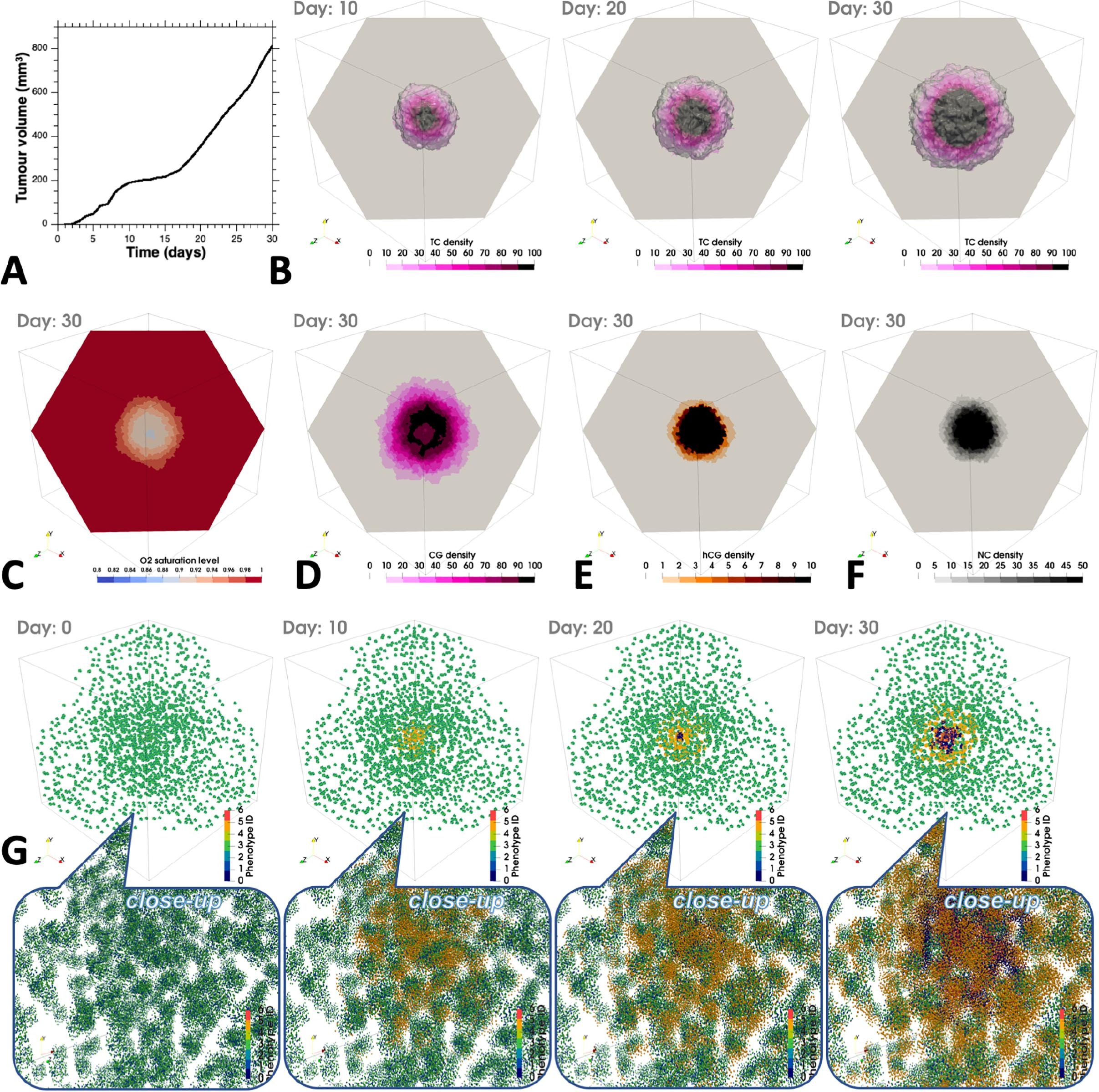
?figurename? A.1: Glioma growth simulation combining an agent-based and continuum-based model from Jean de Montigny et al. [8]. Figure taken from [8] without modification and used under CC BY 4.0.

I supervised Jack Jennings on developing additional functionality for BioDynaMo to enable cryogenics simulations [183, 184]. Freezing and thawing cells with high survival rates is essential for several medical applications. The survival rate depends on many factors during the freezing and thawing process, which are time-consuming to test in a wet lab for each cell type. Simulation can remedy this challenge. The work adds support for heat transfer and osmotic cell membrane properties.

I cooperated with Tobias Duswald on calibrating pyramidal cells, i.e., neurons from the cerebral cortex, using approximate Bayesian computation [10]. This work aimed to find parameter distributions that most likely lead to specific observables, in this case, 3D neuron geometries. To this extent, we integrated BioDynaMo with the tool SMCABC (Sequential Monte Carlo Approximate Bayesian Computation) [558], focusing on reducing the overhead of simulation startup. With this issue addressed, we could execute high-throughput calibration studies with 50 million individual simulations, which not only output parameters that lead to specific geometries but also quantify the uncertainties.

With Ahmad Hesam, I worked on a country-scale COVID simulation demonstrating BioDynaMo’s performance translates into more accurate models [87]. The work builds upon a model where one agent represents 100 persons. This simplification was necessary to allow for simulation execution within a reasonable time. With BioDynaMo’s superior performance characteristics, we were able to lift this restriction and achieve a one-to-one mapping between agents and persons for the whole Dutch population of 17 million people. This high resolution also allows the integration of individual-based data (i.e., microdata) from the Dutch National Statistics Bureau, improving the model accuracy by 38% and explaining hospital admission at a subnational level.

A similar research direction was taken in collaboration with Tobias Duswald and Janne Estill to accelerate an R-based model that simulates the spatial spread of HIV in Malawi [116]. The key issue of this work is the long model execution time of several hours, which prevents meaningful parameter optimization or sensitivity analysis. In this collaboration, we re-implemented the model in BioDynaMo [182]. Our preliminary evaluation shows impressive performance gains in which a BioDynaMo simulation runs in only minutes.

?appendixname? B Complete List of the Author’s Contributions

This section contains a list of contributions that were led by the author (Section B.1), and those as a co-author (Section B.1) in reverse chronological order.

B.1 Contributions Led by the Author

• Lukas Breitwieser, Ahmad Hesam, Abdullah Giray Yaglikci, Mohammad Sadrosadati, Fons Rademakers, and Onur Mutlu. 2024. TeraAgent: A Distributed Agent-Based Simulation Engine for Simulating Half a Trillion Agents. Manuscript to be submitted to: the International Conference for High Performance Computing, Networking, Storage, and Analysis (St. Louis, MO, USA) (SC ’25).

• Lukas Breitwieser, Ahmad Hesam, Fons Rademakers, Juan Gómez Luna, and Onur Mutlu. 2023. High-Performance and Scalable Agent-Based Simulation with BioDynaMo. In Proceedings of the 28th ACM SIGPLAN Annual Symposium on Principles and Practice of Parallel Programming (Montreal, QC, Canada) (PPoPP ’23). Association for Computing Machinery, New York, NY, USA, 174–188. https://doi.org/10.1145/3572848.3577480 arXiv:2301.06984 [cs.DC]
  Supplementary Materials: https://doi.org/10.5281/zenodo.5121618

• Lukas Breitwieser, Ahmad Hesam, Jean de Montigny, Vasileios Vavourakis, Alexandros Iosif, Jack Jennings, Marcus Kaiser, Marco Manca, Alberto Di Meglio, Zaid Al-Ars, Fons Rademakers, Onur Mutlu, and Roman Bauer. 2021. BioDynaMo: a modular platform for high-performance agent-based simulation. Bioinformatics 38, 2 (09 2021), 453–460. https://doi.org/10.1093/bioinformatics/btab649
  Supplementary Materials: https://doi.org/10.5281/zenodo.6463816

B.2 Other Contributions

• Tobias Duswald, Lukas Breitwieser, Thomas Thorne, Barbara Wohlmuth, and Roman Bauer. 2024a. Calibration of stochastic, agent-based neuron growth models with approximate Bayesian computation. Journal of Mathematical Biology 89, 5 (08 Oct 2024), 50. https://doi.org/10.1007/s00285-024-02144-2

• Ahmad Hesam, Frank P Pijpers, Lukas Breitwieser, Peter Hofstee, and Zaid Al-Ars. 2024. Country-Wide Agent-Based Epidemiological Modeling Using 17 Million Individual-Level Microdata. medRxiv (2024). https://doi.org/10.1101/2024.05.27.24307982

• Jack L. Jennings, Sanja Bojic, Lukas Breitweiser, Alex Sharp, and Roman Bauer. 2022. Computational modelling and optimisation of slow cooling profiles for the cryopreservation of cells in suspension. Cryobiology 109 (Dec. 2022), 21–22. https://doi.org/10.1016/j.cryobiol.2022.11.068

• Jean de Montigny, Alexandros Iosif, Lukas Breitwieser, Marco Manca, Roman Bauer, and Vasileios Vavourakis. 2021b. An in silico hybrid continuum-/agent-based procedure to modelling cancer development: Interrogating the interplay amongst glioma invasion, vascularity and necrosis. Methods 185 (2021), 94–104. https://doi.org/10.1016/j.ymeth.2020.01.006 Methods on simulation in biomedicine.

• Ahmad Hesam, Lukas Breitwieser, Fons Rademakers, and Zaid Al-Ars. 2021. GPU Acceleration of 3D Agent-Based Biological Simulations. In 2021 IEEE International Parallel and Distributed Processing Symposium Workshops (IPDPSW). IEEE, New York, NY, USA, 210–217. https://doi.org/10.1109/IPDPSW52791.2021.00040

• Jack Jennings, Roman Bauer, and Lukas Breitwieser. 2019. Computational Modelling Of Slow Freezing Using The Biodynamo Software Package Cryodynamo. Cryobiology 91 (2019), 191–192. https://doi.org/10.1016/j.cryobiol.2019.10.175

?appendixname? C Selected BioDynaMo Simulations Without the Author’s Involvement

This section shows selected simulation visualizations from BioDynaMo users, without the author’s involvement (Figure C.1–C.7). The simulations demonstrate that the functionality provided in the BioDynaMo platform can be used to model dynamic systems whose complexity exceeds the presented use cases in this dissertation.

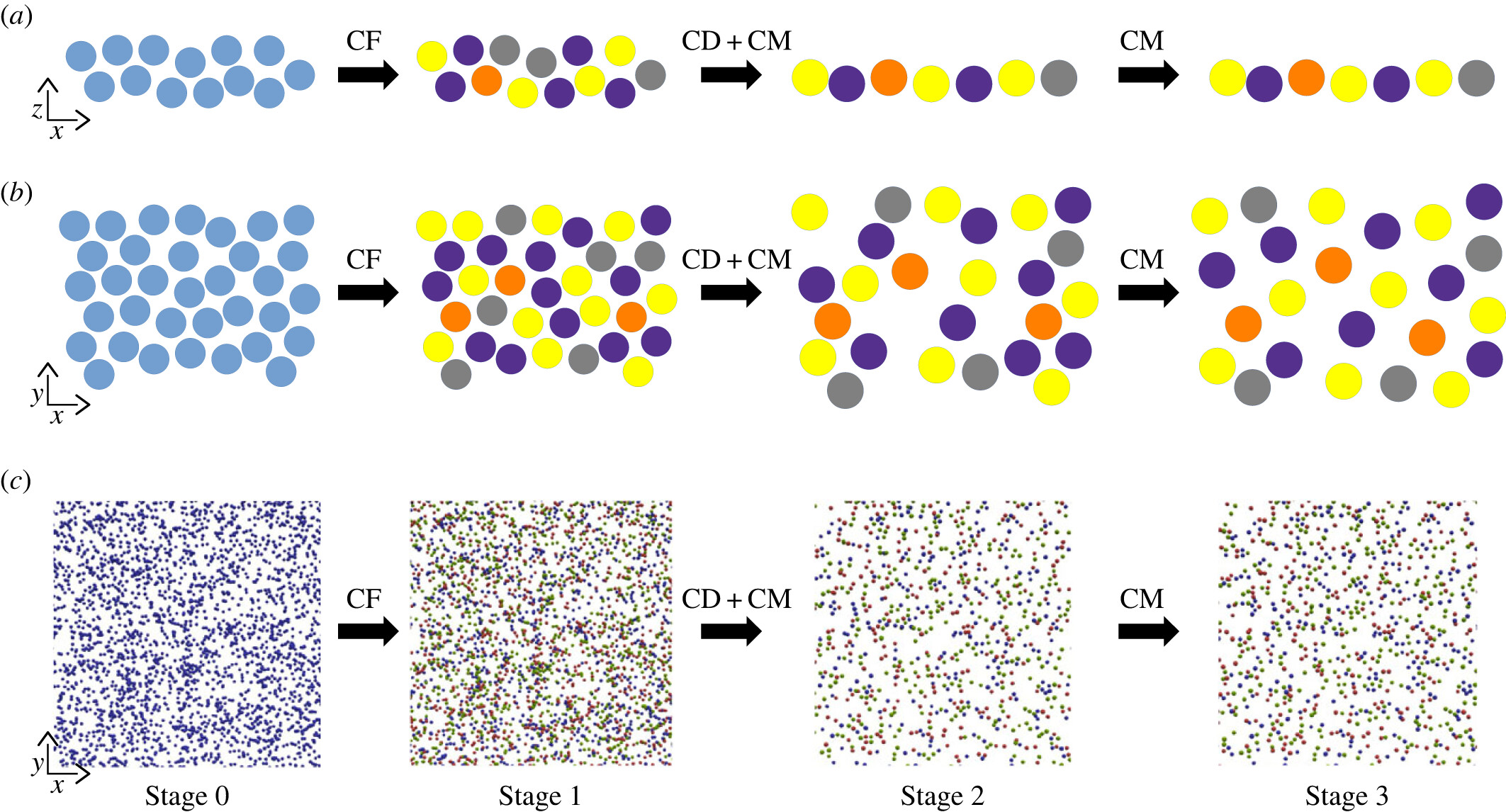
?figurename? C.1: Retinal mosaics are a specific spatial configuration of cells essential for the eye’s function. This model from Jean de Montigny et al. simulates different mechanisms that could be responsible for the development of retinal mosaics [9]. CF: cell fate, CD: cell death, CM: cell migration. Figure taken from [9] without modification and used under CC BY-SA 4.0.

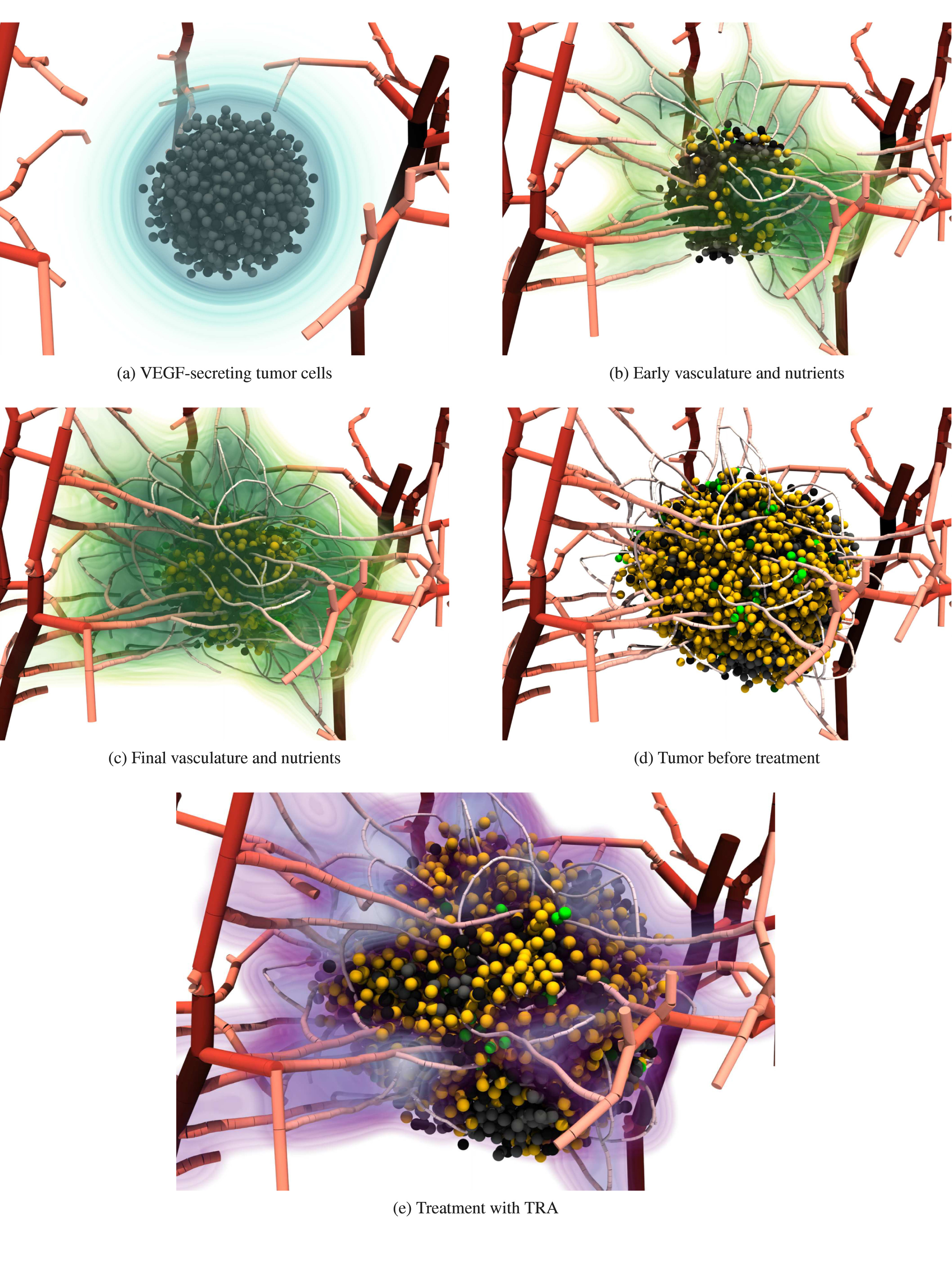
?figurename? C.2: Model simulating vascular tumor growth and treatment from Tobias Duswald et al. [10]. Figure taken from [10] without modification and used under CC BY 4.0.

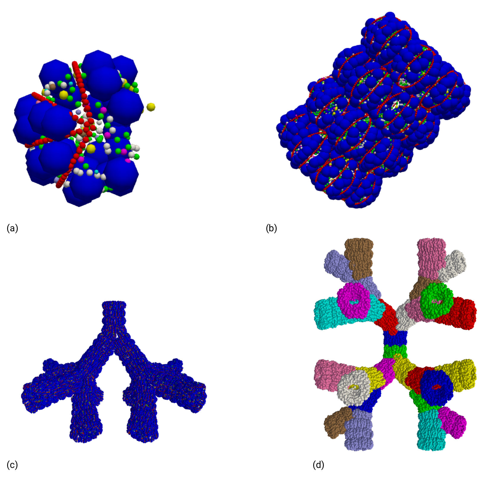
?figurename? C.3: Lung tissue model from Nicolò Cogno’s dissertation [11] about radiation-induced lung injuries. (a) Alveolus with nine different cell types, (b) alveolar segment, pulmonary acinus from the front (c), and bottom (d) [11]. This work was recognized by PhysicsWorld as one of the top 10 breakthroughs in physics in 2024 [12]. Figure taken from [11] without modification and used under CC BY-SA 4.0.

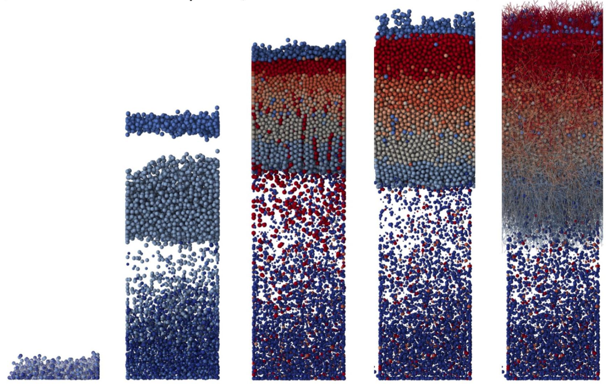
?figurename? C.4: Development of the cerebral cortex from Umar Abubacar and Roman Bauer [13]. Figure taken from [14] and used under CC BY 4.0. The figure was extracted from a collage of different agent-based simulation visualizations.

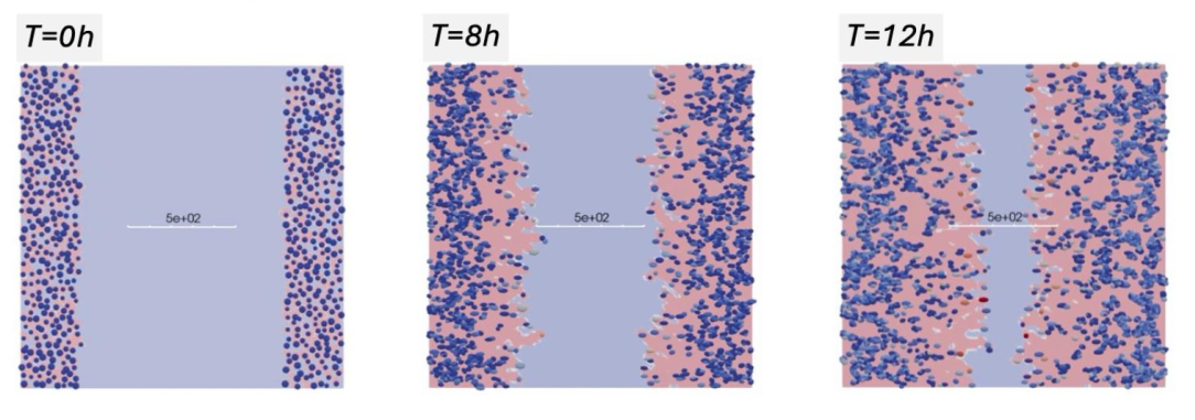
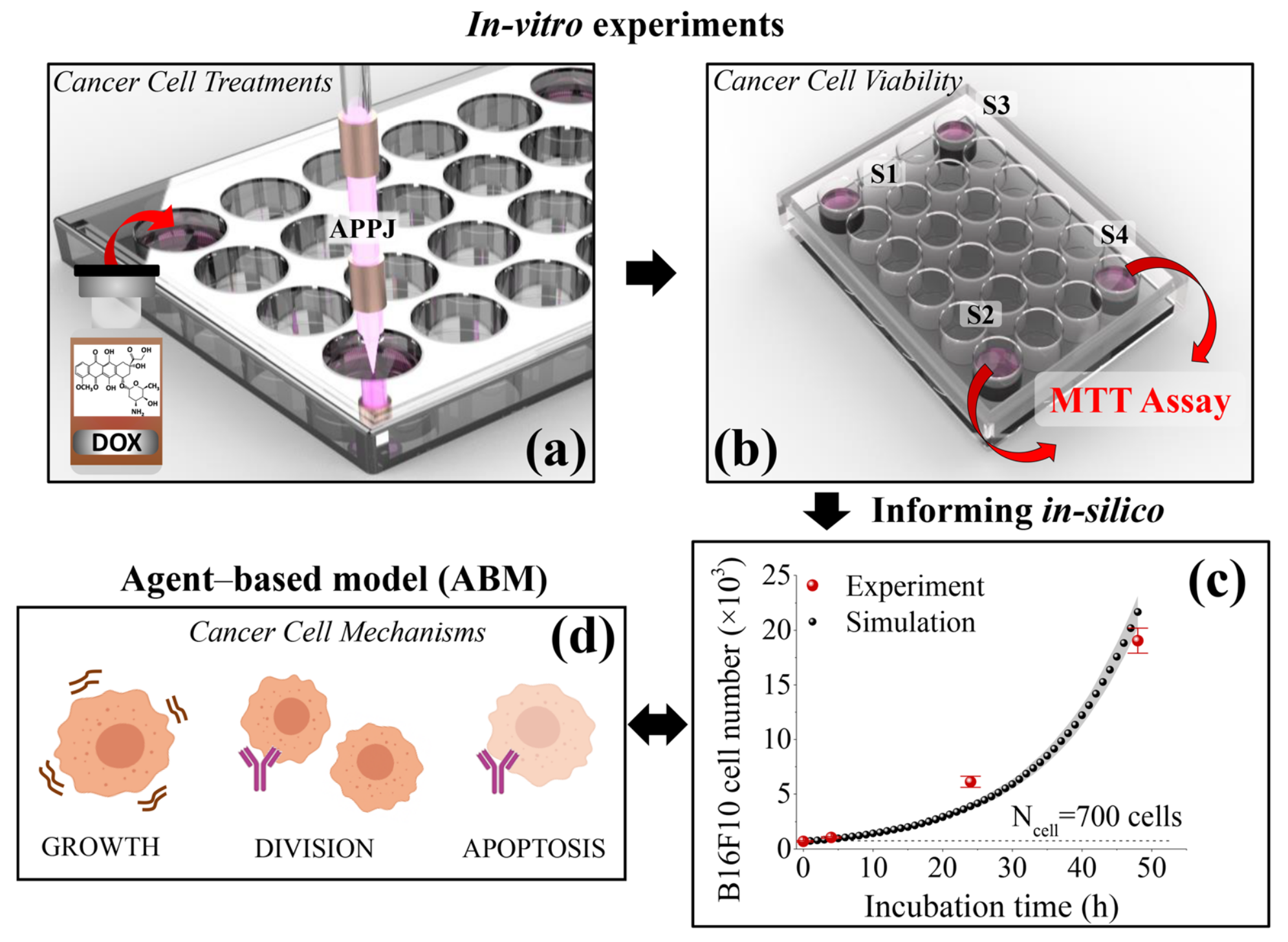
?figurename? C.5: Wound healing simulation by Vasileios Vavourakis, which was inspired by the work of [15]. A video of the simulation is available at [16]. Figure taken from [14] and used under CC BY 4.0. The figure was extracted from a collage of different agent-based simulation visualizations.

?figurename? C.6: In silico study of cancer cell treatment with a helium plasma jet (APPJ) and the doxyrobucin drug (DOX) from Kristaq Gazeli et al. [17]. Figure taken from [17] without modification and used under CC BY 4.0.

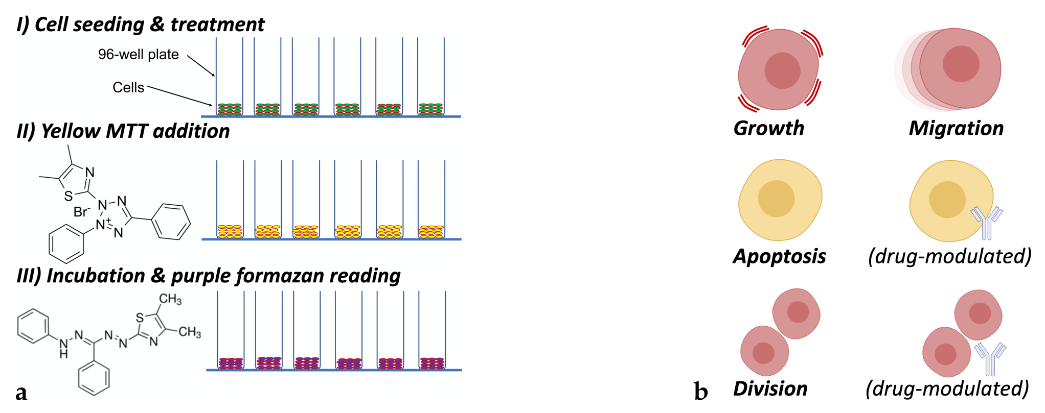
?figurename? C.7: Overview of the work of Marios Demetriades et al. [18] to study cancer drug pharmacodynamics by combining in vitro (a) and in silico (b) methods. Figure taken from [18] without modification and used under CC BY 4.0.

?appendixname? D List of Agents, Events, and Operations

?tablename? D.1: List of agents, events, and operations that BioDynaMo currently provides.

	Description
Agents
Agent	Agent is the base class for all agents in BioDynaMo. This class has a unique id that remains constant during the whole simulation and a collection of behaviors that have been attached to this agent. Agent contains functions to manage behaviors, and to remove itself from the simulation.
SphericalAgent	SphericalAgent extends Agent and adds a spherical agent geometry.
Cell	Cell extends Agent and represents a generic cell with a spherical shape. It includes attributes to describe its geometry, density, and adherence. Cell provides member functions to change its volume, move it in space, calculate mechanical forces, and divide it into two daughter cells. This cell division function creates a new daughter cell and distributes the volume of the mother cell according to the volume ratio parameter. The position of the daughter cell is determined based on the division axis.
NeuronSoma	NeuronSoma extends Cell. This class represents the cell body of a neuron and, like Cell, has a spherical shape. NeuronSoma has a list of neurite elements that extend from the cell body together with their attachment points. NeuronSoma adds a function to extend a new neurite element from the soma. This function takes two parameters: the diameter of the new neurite element, and the orientation of the cylinder in spherical coordinates. [39] contains more details.
NeuriteElement	NeuriteElement extends Agent and has a cylindrical shape with a proximal and distal end. A dendrite is modeled as a binary tree of neurite elements that are internally connected with springs to transmit forces to its proximal connection. The proximal connection can be a NeuriteSoma or a NeuriteElement. This class contains attributes to describe the cylindrical geometry, the spring, pointers to its proximal and distal connections, density, and adherence. A NeuriteElement can elongate, retract, split, branch, bifurcate, and extend a new side neurite. The following list describes these functions in more detail. • Split neurite element. This function splits a neurite element into two segments. The neurite element whose split neurite element function was called becomes the distal one. The new neurite element will be the proximal one. • Extend side neurite. This function adds a side neurite, if one of the distal connections is empty. • Bifurcate. This function creates two new neurite elements and assigns them to the distal connections. This function can only be called for terminal neurite segments because both connections must be empty. • Branch. This function splits the current neurite element into two elements and adds a new side branch at the proximal segment. It is, therefore, a combination of split neurite element and extend side neurite. [39] contains more details.
Behaviors
Chemotaxis	This behavior moves agents along the diffusion gradient (from low concentration to high).
Secretion	This behavior increases the substance concentration at the position of the agent.
GrowthDivision	This behavior grows cells to a specific size and divides them if they exceed the threshold.
GeneRegulation	This behavior calculates protein concentrations which are defined as differential equations.
StatelessBehavior	This behavior reduces the amount of code that has to be written for behaviors without attributes.
Agent operations
BehaviorOp	This operation runs all behaviors which are attached to the agent.
BoundSpaceOp	This operation enforces the space boundary condition (see Section 4.4.11) which can be open, closed or toroidal.
DiscretizationOp	This operation calls the agent’s discretization function. NeuriteElement uses this function to split itself if it becomes too long, or merge with another segment if it is too short.
MechanicalForcesOp	This operation calls the agent’s calculate displacement function and moves the agent accordingly. The calculate displacement function contains the implementation how an agent moves based on all forces that act on it.
Standalone operations
DiffusionOp	This operation calls the update function of all substances in the simulation.
UpdateEnvironmentOp	This operation calls the update function of the environment algorithm.
UpdateTimeSeriesOp	This operation calls the update function of the TimeSeries object which collects relevant data from the current iteration which can be analysed at the end of the simulation.
VisualizationOp	This operation updates the live visualization or generates visualization files for later analysis.

?appendixname? E Supplementary Tutorials

pagecommand=

See pages - of ST01-model-initializer.pdf

See pages - of ST02-user-defined-random-number-distribution.pdf

See pages - of ST03-agent-reproduction-mortality.pdf

See pages - of ST04-agent-reproduction-with-behaviors.pdf

See pages - of ST05-agent-reproduction-advanced.pdf

See pages - of ST06-environment-search.pdf

See pages - of ST07-multi-scale-simulation.pdf

See pages - of ST08-histograms.pdf

See pages - of ST09-timeseries-plotting-basic.pdf

See pages - of ST10-timeseries-plotting-and-analysis.pdf

See pages - of ST11-multiple-experiments-statistical-analysis.pdf

See pages - of ST12-hierarchical-model.pdf

See pages - of ST13-dynamic-scheduling.pdf

See pages - of ST14-randomize-iteration-order.pdf

See pages - of ST15-replace-interaction-force.pdf

- [1]
- Retzlaff et al. [2021] Carl Orge Retzlaff, Martina Ziefle, and André Calero Valdez. 2021. The History of Agent-Based Modeling in the Social Sciences . In Digital Human Modeling and Applications in Health, Safety, Ergonomics and Risk Management. Human Body, Motion and Behavior, Vincent G. Duffy (Ed.). Springer International Publishing, Cham, 304–319. https://doi.org/10.1007/978-3-030-77817-0_22
- Cipresso [2015] Pietro Cipresso. 2015. Modeling behavior dynamics using computational psychometrics within virtual worlds. Frontiers in Psychology 6 (Nov. 2015). https://doi.org/10.3389/fpsyg.2015.01725 Publisher: Frontiers.
- Commons [2024] Wikimedia Commons. 2024. Monte Carlo method applied to approximating the value of . https://en.wikipedia.org/wiki/Monte_Carlo_method#/media/File:Pi_monte_carlo_all.gif Accessed on September 26, 2024.
- Mellström et al. [2016] Britt Mellström, Asta Kastanauskaite, Shira Knafo, Paz Gonzalez, Xose M. Dopazo, Ana Ruiz-Nuño, John G. R. Jefferys, Min Zhuo, Tim V. P. Bliss, Jose R. Naranjo, and Javier DeFelipe. 2016. Specific cytoarchitectureal changes in hippocampal subareas in daDREAM mice. Molecular Brain 9, 1 (Dec. 2016). https://doi.org/10.1186/s13041-016-0204-8
- Gong et al. [2015] Xue Gong, Chao Lin, Jian Cheng, Jiansheng Su, Hang Zhao, Tianlin Liu, Xuejun Wen, and Peng Zhao. 2015. Generation of Multicellular Tumor Spheroids with Microwell-Based Agarose Scaffolds for Drug Testing. PLOS ONE 10, 6 (06 2015), 1–18. https://doi.org/10.1371/journal.pone.0130348
- Kang et al. [2014] Seunghwa Kang, Simon Kahan, Jason McDermott, Nicholas Flann, and Ilya Shmulevich. 2014. Biocellion: accelerating computer simulation of multicellular biological system models. Bioinformatics 30, 21 (Nov. 2014), 3101–3108. https://doi.org/10.1093/bioinformatics/btu498
- de Montigny et al. [2021] Jean de Montigny, Alexandros Iosif, Lukas Breitwieser, Marco Manca, Roman Bauer, and Vasileios Vavourakis. 2021. An in silico hybrid continuum-/agent-based procedure to modelling cancer development: Interrogating the interplay amongst glioma invasion, vascularity and necrosis. Methods 185 (2021), 94–104. https://doi.org/10.1016/j.ymeth.2020.01.006 Methods on simulation in biomedicine.
- de Montigny et al. [2023] Jean de Montigny, Evelyne Sernagor, and Roman Bauer. 2023. Retinal self-organization: a model of retinal ganglion cells and starburst amacrine cells mosaic formation. Open Biology 13, 4 (April 2023), 220217. https://doi.org/10.1098/rsob.220217 Publisher: Royal Society.
- Duswald et al. [2024] Tobias Duswald, Ernesto A.B.F. Lima, J. Tinsley Oden, and Barbara Wohlmuth. 2024. Bridging scales: A hybrid model to simulate vascular tumor growth and treatment response. Computer Methods in Applied Mechanics and Engineering 418 (2024), 116566. https://doi.org/10.1016/j.cma.2023.116566
- Cogno [2023] Nicolò Cogno. 2023. Agent-Based Modelling of Radiation-Induced Lung Injuries. Ph. D. Dissertation. Technische Universität Darmstadt, Darmstadt. https://doi.org/10.26083/tuprints-00026335
- Hamish Johnston [2024] Hamish Johnston. 2024. Top 10 Breakthroughs of the Year in physics for 2024 revealed. https://physicsworld.com/a/top-10-breakthroughs-of-the-year-in-physics-for-2024-revealed/
- Abubacar and Bauer [2024] Umar Abubacar and Roman Bauer. 2024 (acccessed Aug 26, 2024). Agent-Based Modelling to Simulate Realistic Self-Organizing Development of the Mammalian Cerebral Cortex. https://drive.google.com/file/d/1usV1M4BgKEeEHNQxT3GDDR5uNeipNYt5/view
- Cogno et al. [2024] Nicolò Cogno, Cristian Axenie, Roman Bauer, and Vasileios Vavourakis. 2024. Agent-based modeling in cancer biomedicine: applications and tools for calibration and validation. Cancer Biology & Therapy 25, 1 (Dec. 2024), 2344600. https://doi.org/10.1080/15384047.2024.2344600 Publisher: Taylor & Francis _eprint: https://doi.org/10.1080/15384047.2024.2344600.
- Mascheroni et al. [2019] Pietro Mascheroni, Juan Carlos López Alfonso, Maria Kalli, Triantafyllos Stylianopoulos, Michael Meyer-Hermann, and Haralampos Hatzikirou. 2019. On the Impact of Chemo-Mechanically Induced Phenotypic Transitions in Gliomas. Cancers 11, 5 (May 2019), 716. https://doi.org/10.3390/cancers11050716 Number: 5 Publisher: Multidisciplinary Digital Publishing Institute.
- Vavourakis [2021] Vasileios Vavourakis. 2021. In silico model of A172-cell wound closure assay under 0 mm-Hg compression. https://www.youtube.com/watch?v=8N982C0u44o Accessed on September 26, 2024.
- Gazeli et al. [2022] K. Gazeli, M. Hadjicharalambous, Eleftherios Ioannou, O. Gazeli, C. Lazarou, C. Anastassiou, P. Svarnas, V. Vavourakis, and G. E. Georghiou. 2022. Interrogating an in silico model to determine helium plasma jet and chemotherapy efficacy against B16F10 melanoma cells. Applied Physics Letters 120, 5 (Jan. 2022), 054101. https://doi.org/10.1063/5.0077694
- Demetriades et al. [2022] Marios Demetriades, Marko Zivanovic, Myrianthi Hadjicharalambous, Eleftherios Ioannou, Biljana Ljujic, Ksenija Vucicevic, Zeljko Ivosevic, Aleksandar Dagovic, Nevena Milivojevic, Odysseas Kokkinos, Roman Bauer, and Vasileios Vavourakis. 2022. Interrogating and Quantifying In Vitro Cancer Drug Pharmacodynamics via Agent-Based and Bayesian Monte Carlo Modelling. Pharmaceutics 14, 4 (April 2022), 749. https://doi.org/10.3390/pharmaceutics14040749 Number: 4 Publisher: Multidisciplinary Digital Publishing Institute.
- Axelrod and Hamilton [1981] Robert Axelrod and William D. Hamilton. 1981. The Evolution of Cooperation. Science 211, 4489 (March 1981), 1390–1396. https://doi.org/10.1126/science.7466396 Publisher: American Association for the Advancement of Science.
- Weinzierl [2021] Tobias Weinzierl. 2021. The Pillars of Science. In Principles of Parallel Scientific Computing: A First Guide to Numerical Concepts and Programming Methods, Tobias Weinzierl (Ed.). Springer International Publishing, Cham, 3–9. https://doi.org/10.1007/978-3-030-76194-3_1
- Epstein [2008] Joshua M. Epstein. 2008. Why Model? https://jasss.soc.surrey.ac.uk/11/4/12.html Publisher: JASSS.
- Schelling [1971] Thomas C. Schelling. 1971. Dynamic models of segregation†. The Journal of Mathematical Sociology 1, 2 (1971), 143–186. https://doi.org/10.1080/0022250X.1971.9989794 arXiv:https://doi.org/10.1080/0022250X.1971.9989794
- Cogno et al. [2024] Nicolò Cogno, Roman Bauer, and Marco Durante. 2024. Mechanistic model of radiotherapy-induced lung fibrosis using coupled 3D agent-based and Monte Carlo simulations. Communications Medicine 4, 1 (09 Feb 2024), 16. https://doi.org/10.1038/s43856-024-00442-w
- Cogno et al. [2022a] Nicolò Cogno, Roman Bauer, and Marco Durante. 2022a. An Agent-Based Model of Radiation-Induced Lung Fibrosis. International Journal of Molecular Sciences 23, 22 (Jan. 2022), 13920. https://doi.org/10.3390/ijms232213920 Number: 22 Publisher: Multidisciplinary Digital Publishing Institute.
- Cogno et al. [2022b] Nicolò Cogno, Roman Bauer, and Marco Durante. 2022b. A 3D Agent-Based Model of Lung Fibrosis. Symmetry 14, 1 (Jan. 2022), 90. https://doi.org/10.3390/sym14010090 Number: 1 Publisher: Multidisciplinary Digital Publishing Institute.
- Nicolò Cogno and Vavourakis [2024] Roman Bauer Nicolò Cogno, Cristian Axenie and Vasileios Vavourakis. 2024. Agent-based modeling in cancer biomedicine: applications and tools for calibration and validation. Cancer Biology & Therapy 25, 1 (2024), 2344600. https://doi.org/10.1080/15384047.2024.2344600 arXiv:https://doi.org/10.1080/15384047.2024.2344600 PMID: 38678381.
- Metzcar et al. [2019] John Metzcar, Yafei Wang, Randy Heiland, and Paul Macklin. 2019. A Review of Cell-Based Computational Modeling in Cancer Biology. JCO Clinical Cancer Informatics 3, 3 (Feb. 2019), 1–13. https://doi.org/10.1200/CCI.18.00069 Publisher: Wolters Kluwer.
- Wang et al. [2015] Zhihui Wang, Joseph D. Butner, Romica Kerketta, Vittorio Cristini, and Thomas S. Deisboeck. 2015. Simulating cancer growth with multiscale agent-based modeling. Seminars in Cancer Biology 30 (Feb. 2015), 70–78. https://doi.org/10.1016/j.semcancer.2014.04.001
- Olsen and Siegelmann [2013] Megan M. Olsen and Hava T. Siegelmann. 2013. Multiscale Agent-based Model of Tumor Angiogenesis. Procedia Computer Science 18 (Jan. 2013), 1016–1025. https://doi.org/10.1016/j.procs.2013.05.267
- Wang et al. [2013] Jun Wang, Le Zhang, Chenyang Jing, Gang Ye, Hulin Wu, Hongyu Miao, Yukun Wu, and Xiaobo Zhou. 2013. Multi-scale agent-based modeling on melanoma and its related angiogenesis analysis. Theoretical Biology and Medical Modelling 10, 1 (June 2013), 41. https://doi.org/10.1186/1742-4682-10-41
- An and Kulkarni [2015] Gary An and Swati Kulkarni. 2015. An agent-based modeling framework linking inflammation and cancer using evolutionary principles: Description of a generative hierarchy for the hallmarks of cancer and developing a bridge between mechanism and epidemiological data. Mathematical Biosciences 260 (Feb. 2015), 16–24. https://doi.org/10.1016/j.mbs.2014.07.009
- Wang et al. [2015a] Zhihui Wang, Joseph D. Butner, Vittorio Cristini, and Thomas S. Deisboeck. 2015a. Integrated PK-PD and agent-based modeling in oncology. Journal of Pharmacokinetics and Pharmacodynamics 42, 2 (April 2015), 179–189. https://doi.org/10.1007/s10928-015-9403-7
- Wang et al. [2015b] Zhihui Wang, Joseph D. Butner, Romica Kerketta, Vittorio Cristini, and Thomas S. Deisboeck. 2015b. Simulating cancer growth with multiscale agent-based modeling. Seminars in Cancer Biology 30 (Feb. 2015), 70–78. https://doi.org/10.1016/j.semcancer.2014.04.001
- Poleszczuk et al. [2016] Jan Poleszczuk, Paul Macklin, and Heiko Enderling. 2016. Agent-Based Modeling of Cancer Stem Cell Driven Solid Tumor Growth. In Stem Cell Heterogeneity: Methods and Protocols, Kursad Turksen (Ed.). Springer, New York, NY, 335–346. https://doi.org/10.1007/7651_2016_346
- Norton et al. [2019] Kerri-Ann Norton, Chang Gong, Samira Jamalian, and Aleksander S. Popel. 2019. Multiscale Agent-Based and Hybrid Modeling of the Tumor Immune Microenvironment. Processes 7, 1 (Jan. 2019), 37. https://doi.org/10.3390/pr7010037 Number: 1 Publisher: Multidisciplinary Digital Publishing Institute.
- Heidary et al. [2020] Zarifeh Heidary, Jafar Ghaisari, Shiva Moein, and Shaghayegh Haghjooy Javanmard. 2020. The double-edged sword role of fibroblasts in the interaction with cancer cells; an agent-based modeling approach. PLOS ONE 15, 5 (May 2020), e0232965. https://doi.org/10.1371/journal.pone.0232965 Publisher: Public Library of Science.
- Rivera et al. [2022] Melanie Rivera, Leslie Toledo-Jacobo, Elsa Romero, Tudor I. Oprea, Melanie E. Moses, Laurie G. Hudson, Angela Wandinger-Ness, and Martha M. Grimes. 2022. Agent-based modeling predicts RAC1 is critical for ovarian cancer metastasis. Molecular Biology of the Cell 33, 14 (Dec. 2022), ar138. https://doi.org/10.1091/mbc.E21-11-0540 Publisher: American Society for Cell Biology (mboc).
- van Genderen et al. [2024] Maisa N. G. van Genderen, Jeroen Kneppers, Anniek Zaalberg, Elise M. Bekers, Andries M. Bergman, Wilbert Zwart, and Federica Eduati. 2024. Agent-based modeling of the prostate tumor microenvironment uncovers spatial tumor growth constraints and immunomodulatory properties. npj Systems Biology and Applications 10, 1 (Feb. 2024), 1–13. https://doi.org/10.1038/s41540-024-00344-6 Publisher: Nature Publishing Group.
- Zubler and Douglas [2009] Frederic Zubler and Rodney Douglas. 2009. A framework for modeling the growth and development of neurons and networks. Frontiers in computational neuroscience 3 (2009), 25. https://doi.org/10.3389/neuro.10.025.2009
- Zubler [2009] Frédéric Zubler. 2009. Simulation of corticogenesis as a self-organizing system. Dissertation. University of Zurich, Zürich. https://doi.org/10.5167/uzh-164111 ISSN: 2012-1415 Publication Title: Zubler, Frédéric. Simulation of corticogenesis as a self-organizing system. 2009, University of Zurich, Faculty of Science..
- Duswald et al. [2024] Tobias Duswald, Lukas Breitwieser, Thomas Thorne, Barbara Wohlmuth, and Roman Bauer. 2024. Calibration of stochastic, agent-based neuron growth models with approximate Bayesian computation. Journal of Mathematical Biology 89, 5 (08 Oct 2024), 50. https://doi.org/10.1007/s00285-024-02144-2 arXiv:2405.13905 [cs.CE]
- Torben-Nielsen and De Schutter [2014] Benjamin Torben-Nielsen and Erik De Schutter. 2014. Context-aware modeling of neuronal morphologies. Frontiers in Neuroanatomy 8 (Sept. 2014). https://doi.org/10.3389/fnana.2014.00092
- De Schutter [2023] Erik De Schutter. 2023. Efficient simulation of neural development using shared memory parallelization. Frontiers in Neuroinformatics 17 (2023). https://www.frontiersin.org/articles/10.3389/fninf.2023.1212384
- Pennisi et al. [2015] Marzio Pennisi, Giulia Russo, Santo Motta, and Francesco Pappalardo. 2015. Agent based modeling of the effects of potential treatments over the blood–brain barrier in multiple sclerosis. Journal of Immunological Methods 427 (Dec. 2015), 6–12. https://doi.org/10.1016/j.jim.2015.08.014
- Caffrey et al. [2014] James R. Caffrey, Barry D. Hughes, Joanne M. Britto, and Kerry A. Landman. 2014. An In Silico Agent-Based Model Demonstrates Reelin Function in Directing Lamination of Neurons during Cortical Development. PLOS ONE 9, 10 (Oct. 2014), e110415. https://doi.org/10.1371/journal.pone.0110415 Publisher: Public Library of Science.
- Avin et al. [2021] Shahar Avin, Adrian Currie, and Stephen H. Montgomery. 2021. An agent-based model clarifies the importance of functional and developmental integration in shaping brain evolution. BMC Biology 19, 1 (May 2021), 97. https://doi.org/10.1186/s12915-021-01024-1
- Glen et al. [2019] Chad M. Glen, Melissa L. Kemp, and Eberhard O. Voit. 2019. Agent-based modeling of morphogenetic systems: Advantages and challenges. PLOS Computational Biology 15, 3 (March 2019), e1006577. https://doi.org/10.1371/journal.pcbi.1006577 Publisher: Public Library of Science.
- Tang et al. [2011] Jonathan Tang, Heiko Enderling, Sabine Becker-Weimann, Christopher Pham, Aris Polyzos, Chen-Yi Chen, and Sylvain V. Costes. 2011. Phenotypic transition maps of 3D breast acini obtained by imaging-guided agent-based modeling. Integrative Biology 3, 4 (April 2011), 408–421. https://doi.org/10.1039/c0ib00092b
- Lambert et al. [2018] Ben Lambert, Adam L. MacLean, Alexander G. Fletcher, Alexander N. Combes, Melissa H. Little, and Helen M. Byrne. 2018. Bayesian inference of agent-based models: a tool for studying kidney branching morphogenesis. Journal of Mathematical Biology 76, 7 (June 2018), 1673–1697. https://doi.org/10.1007/s00285-018-1208-z
- Walpole et al. [2015] J. Walpole, J. C. Chappell, J. G. Cluceru, F. Mac Gabhann, V. L. Bautch, and S. M. Peirce. 2015. Agent-based model of angiogenesis simulates capillary sprout initiation in multicellular networks. Integrative Biology 7, 9 (Sept. 2015), 987–997. https://doi.org/10.1039/c5ib00024f
- Camacho-Gómez et al. [2022] Daniel Camacho-Gómez, José Manuel García-Aznar, and María José Gómez-Benito. 2022. A 3D multi-agent-based model for lumen morphogenesis: the role of the biophysical properties of the extracellular matrix. Engineering with Computers 38, 5 (Oct. 2022), 4135–4149. https://doi.org/10.1007/s00366-022-01654-1
- Dalle Nogare and Chitnis [2020] Damian Dalle Nogare and Ajay B Chitnis. 2020. NetLogo agent-based models as tools for understanding the self-organization of cell fate, morphogenesis and collective migration of the zebrafish posterior Lateral Line primordium. Seminars in Cell & Developmental Biology 100 (April 2020), 186–198. https://doi.org/10.1016/j.semcdb.2019.12.015
- Bonabeau [1997] Eric Bonabeau. 1997. From Classical Models of Morphogenesis to Agent-Based Models of Pattern Formation. Artificial Life 3, 3 (July 1997), 191–211. https://doi.org/10.1162/artl.1997.3.3.191
- Thorne et al. [2007] Bryan C. Thorne, Alexander M. Bailey, Douglas W. DeSimone, and Shayn M. Peirce. 2007. Agent-based modeling of multicell morphogenic processes during development. Birth Defects Research Part C: Embryo Today: Reviews 81, 4 (2007), 344–353. https://doi.org/10.1002/bdrc.20106 _eprint: https://onlinelibrary.wiley.com/doi/pdf/10.1002/bdrc.20106.
- Kreft et al. [2001] Jan-Ulrich Kreft, Cristian Picioreanu, Julian W. T. Wimpenny, and Mark C. M. van Loosdrecht. 2001. Individual-based modelling of biofilms. Microbiology 147, 11 (2001), 2897–2912. https://doi.org/10.1099/00221287-147-11-2897 Publisher: Microbiology Society,.
- Wilmoth et al. [2018] Jared L. Wilmoth, Peter W. Doak, Andrea Timm, Michelle Halsted, John D. Anderson, Marta Ginovart, Clara Prats, Xavier Portell, Scott T. Retterer, and Miguel Fuentes-Cabrera. 2018. A Microfluidics and Agent-Based Modeling Framework for Investigating Spatial Organization in Bacterial Colonies: The Case of Pseudomonas Aeruginosa and H1-Type VI Secretion Interactions. Frontiers in Microbiology 9 (Feb. 2018). https://doi.org/10.3389/fmicb.2018.00033 Publisher: Frontiers.
- Li et al. [2024] Changhao Li, Japinder Nijjer, Luyi Feng, Qiuting Zhang, Jing Yan, and Sulin Zhang. 2024. Agent-based modeling of stress anisotropy driven nematic ordering in growing biofilms. Soft Matter 20, 16 (2024), 3401–3410. https://doi.org/10.1039/D3SM01535A Publisher: Royal Society of Chemistry.
- Latif and May [2018] Majid Latif and Elebeoba E. May. 2018. A Multiscale Agent-Based Model for the Investigation of E . coli K12 Metabolic Response During Biofilm Formation. Bulletin of Mathematical Biology 80, 11 (Nov. 2018), 2917–2956. https://doi.org/10.1007/s11538-018-0494-3
- Sweeney et al. [2019] Emily G. Sweeney, Andrew Nishida, Alexandra Weston, Maria S. Bañuelos, Kristin Potter, John Conery, and Karen Guillemin. 2019. Agent-Based Modeling Demonstrates How Local Chemotactic Behavior Can Shape Biofilm Architecture. mSphere 4, 3 (May 2019), 10.1128/msphere.00285–19. https://doi.org/10.1128/msphere.00285-19 Publisher: American Society for Microbiology.
- Nagarajan et al. [2022] Karthik Nagarajan, Congjian Ni, and Ting Lu. 2022. Agent-Based Modeling of Microbial Communities. ACS Synthetic Biology 11, 11 (Nov. 2022), 3564–3574. https://doi.org/10.1021/acssynbio.2c00411 Publisher: American Chemical Society.
- Koshy-Chenthittayil et al. [2021] Sherli Koshy-Chenthittayil, Linda Archambault, Dhananjai Senthilkumar, Reinhard Laubenbacher, Pedro Mendes, and Anna Dongari-Bagtzoglou. 2021. Agent Based Models of Polymicrobial Biofilms and the Microbiome—A Review. Microorganisms 9, 2 (Feb. 2021), 417. https://doi.org/10.3390/microorganisms9020417 Number: 2 Publisher: Multidisciplinary Digital Publishing Institute.
- Montealegre and Rammig [2012] Norma Montealegre and Franz J. Rammig. 2012. Agent-Based Modeling and Simulation of Artificial Immune Systems. In 2012 IEEE 15th International Symposium on Object/ Component/Service-Oriented Real-Time Distributed Computing Workshops. 212–219. https://doi.org/10.1109/ISORCW.2012.43
- Shinde and Kurhekar [2018] Snehal B. Shinde and Manish P. Kurhekar. 2018. Review of the systems biology of the immune system using agent-based models. IET Systems Biology 12, 3 (2018), 83–92. https://doi.org/10.1049/iet-syb.2017.0073 _eprint: https://onlinelibrary.wiley.com/doi/pdf/10.1049/iet-syb.2017.0073.
- Bauer et al. [2009] Amy L. Bauer, Catherine A. A. Beauchemin, and Alan S. Perelson. 2009. Agent-based modeling of host–pathogen systems: The successes and challenges. Information Sciences 179, 10 (April 2009), 1379–1389. https://doi.org/10.1016/j.ins.2008.11.012
- Truszkowska et al. [2022] Agnieszka Truszkowska, Lorenzo Zino, Sachit Butail, Emanuele Caroppo, Zhong-Ping Jiang, Alessandro Rizzo, and Maurizio Porfiri. 2022. Predicting the Effects of Waning Vaccine Immunity Against COVID-19 through High-Resolution Agent-Based Modeling. Advanced Theory and Simulations 5, 6 (2022), 2100521. https://doi.org/10.1002/adts.202100521 _eprint: https://onlinelibrary.wiley.com/doi/pdf/10.1002/adts.202100521.
- Perrin et al. [2006] Dimitri Perrin, Heather J. Ruskin, John Burns, and Martin Crane. 2006. An Agent-Based Approach to Immune Modelling. In Computational Science and Its Applications - ICCSA 2006, Marina Gavrilova, Osvaldo Gervasi, Vipin Kumar, C. J. Kenneth Tan, David Taniar, Antonio Laganá, Youngsong Mun, and Hyunseung Choo (Eds.). Springer, Berlin, Heidelberg, 612–621. https://doi.org/10.1007/11751540_65
- Pappalardo et al. [2018] Francesco Pappalardo, Giulia Russo, Marzio Pennisi, Giuseppe Sgroi, Giuseppe Alessandro Parasiliti Palumbo, Santo Motta, and Epifanio Fichera. 2018. An agent based modeling approach for the analysis of tuberculosis – immune system dynamics. In 2018 IEEE International Conference on Bioinformatics and Biomedicine (BIBM). 1386–1392. https://doi.org/10.1109/BIBM.2018.8621355
- Folcik et al. [2011] Virginia A. Folcik, Gordon Broderick, Shunmugam Mohan, Brian Block, Chirantan Ekbote, John Doolittle, Marc Khoury, Luke Davis, and Clay B. Marsh. 2011. Using an agent-based model to analyze the dynamic communication network of the immune response. Theoretical Biology and Medical Modelling 8, 1 (Jan. 2011), 1. https://doi.org/10.1186/1742-4682-8-1
- Folcik et al. [2007] Virginia A. Folcik, Gary C. An, and Charles G. Orosz. 2007. The Basic Immune Simulator: An agent-based model to study the interactions between innate and adaptive immunity. Theoretical Biology and Medical Modelling 4, 1 (Sept. 2007), 39. https://doi.org/10.1186/1742-4682-4-39
- Chiacchio et al. [2014] Ferdinando Chiacchio, Marzio Pennisi, Giulia Russo, Santo Motta, and Francesco Pappalardo. 2014. Agent-Based Modeling of the Immune System: NetLogo, a Promising Framework. BioMed Research International 2014, 1 (2014), 907171. https://doi.org/10.1155/2014/907171 _eprint: https://onlinelibrary.wiley.com/doi/pdf/10.1155/2014/907171.
- Jacob et al. [2011] Christian Jacob, Vladimir Sarpe, Carey Gingras, and Rolando Pajon Feyt. 2011. Swarm-Based Simulations for Immunobiology. In Information Processing and Biological Systems, Samuli Niiranen and Andre Ribeiro (Eds.). Springer, Berlin, Heidelberg, 29–64. https://doi.org/10.1007/978-3-642-19621-8_3
- Li [2016] Yan Li. 2016. Agent-Based Modeling of Chronic Diseases: A Narrative Review and Future Research Directions. Preventing Chronic Disease 13 (2016). https://doi.org/10.5888/pcd13.150561
- Montagna and Omicini [2017] Sara Montagna and Andrea Omicini. 2017. Agent-based modeling for the self-management of chronic diseases: An exploratory study. SIMULATION 93, 9 (Sept. 2017), 781–793. https://doi.org/10.1177/0037549717712605 Publisher: SAGE Publications Ltd STM.
- Nianogo and Arah [2015] Roch A. Nianogo and Onyebuchi A. Arah. 2015. Agent-Based Modeling of Noncommunicable Diseases: A Systematic Review. American Journal of Public Health 105, 3 (March 2015), e20–e31. https://doi.org/10.2105/AJPH.2014.302426 Publisher: American Public Health Association.
- Schryver et al. [2015] Jack Schryver, James Nutaro, and Mallikarjun Shankar. 2015. Emulating a System Dynamics Model with Agent-Based Models : A Methodological Case Study in Simulation of Diabetes Progression. Open Journal of Modelling and Simulation 03, 04 (Oct. 2015). https://doi.org/10.4236/ojmsi.2015.34019 Institution: Oak Ridge National Laboratory (ORNL), Oak Ridge, TN (United States) Publisher: Scientific Research Publishing.
- Mi et al. [2007] Qi Mi, Beatrice Rivière, Gilles Clermont, David L. Steed, and Yoram Vodovotz. 2007. Agent-based model of inflammation and wound healing: insights into diabetic foot ulcer pathology and the role of transforming growth factor-1. Wound Repair and Regeneration 15, 5 (2007), 671–682. https://doi.org/10.1111/j.1524-475X.2007.00271.x _eprint: https://onlinelibrary.wiley.com/doi/pdf/10.1111/j.1524-475X.2007.00271.x.
- Khademi et al. [2018] Amin Khademi, Donglan Zhang, Philippe J. Giabbanelli, Shirley Timmons, Chengqian Luo, and Lu Shi. 2018. An Agent-Based Model of Healthy Eating with Applications to Hypertension. In Advanced Data Analytics in Health, Philippe J. Giabbanelli, Vijay K. Mago, and Elpiniki I. Papageorgiou (Eds.). Springer International Publishing, Cham, 43–58. https://doi.org/10.1007/978-3-319-77911-9_3
- Li et al. [2014] Yan Li, Nan Kong, Mark Lawley, and José A. Pagán. 2014. Assessing lifestyle interventions to improve cardiovascular health using an agent-based model. In Proceedings of the Winter Simulation Conference 2014. 1221–1232. https://doi.org/10.1109/WSC.2014.7019979 ISSN: 1558-4305.
- Archbold et al. [2024] James Archbold, Sophie Clohessy, Deshani Herath, Nathan Griffiths, and Oyinlola Oyebode. 2024. An agent-based model of the spread of behavioural risk-factors for cardiovascular disease in city-scale populations. PLOS ONE 19, 5 (May 2024), e0303051. https://doi.org/10.1371/journal.pone.0303051 Publisher: Public Library of Science.
- Giabbanelli et al. [2021] Philippe J. Giabbanelli, Boone Tison, and James Keith. 2021. The application of modeling and simulation to public health: Assessing the quality of Agent-Based Models for obesity. Simulation Modelling Practice and Theory 108 (April 2021), 102268. https://doi.org/10.1016/j.simpat.2020.102268
- Morshed et al. [2019] Alexandra B. Morshed, Matt Kasman, Benjamin Heuberger, Ross A. Hammond, and Peter S. Hovmand. 2019. A systematic review of system dynamics and agent-based obesity models: Evaluating obesity as part of the global syndemic. Obesity Reviews 20, S2 (2019), 161–178. https://doi.org/10.1111/obr.12877 _eprint: https://onlinelibrary.wiley.com/doi/pdf/10.1111/obr.12877.
- Beheshti et al. [2017] Rahmatollah Beheshti, Mehdi Jalalpour, and Thomas A. Glass. 2017. Comparing methods of targeting obesity interventions in populations: An agent-based simulation. SSM - Population Health 3 (Dec. 2017), 211–218. https://doi.org/10.1016/j.ssmph.2017.01.006
- Giabbanelli and Crutzen [2017] Philippe J. Giabbanelli and Rik Crutzen. 2017. Using Agent-Based Models to Develop Public Policy about Food Behaviours: Future Directions and Recommendations. Computational and Mathematical Methods in Medicine 2017, 1 (2017), 5742629. https://doi.org/10.1155/2017/5742629 _eprint: https://onlinelibrary.wiley.com/doi/pdf/10.1155/2017/5742629.
- Squires et al. [2023] Hazel Squires, Michael P. Kelly, Nigel Gilbert, Falko Sniehotta, and Robin C. Purshouse. 2023. The long-term effectiveness and cost-effectiveness of public health interventions; how can we model behavior? A review. Health Economics 32, 12 (2023), 2836–2854. https://doi.org/10.1002/hec.4754 _eprint: https://onlinelibrary.wiley.com/doi/pdf/10.1002/hec.4754.
- Gao et al. [2017] Hongjie Gao, Zuojing Yin, Zhiwei Cao, and Le Zhang. 2017. Developing an Agent-Based Drug Model to Investigate the Synergistic Effects of Drug Combinations. Molecules 22, 12 (Dec. 2017), 2209. https://doi.org/10.3390/molecules22122209 Number: 12 Publisher: Multidisciplinary Digital Publishing Institute.
- Li et al. [2018] Yan Li, Nan Kong, Mark A. Lawley, and José A. Pagán. 2018. An Agent-Based Model for Ideal Cardiovascular Health. In Decision Analytics and Optimization in Disease Prevention and Treatment. John Wiley & Sons, Ltd, 241–258. https://doi.org/10.1002/9781118960158.ch11 Section: 11 _eprint: https://onlinelibrary.wiley.com/doi/pdf/10.1002/9781118960158.ch11.
- Hesam et al. [2024] Ahmad Hesam, Frank P Pijpers, Lukas Breitwieser, Peter Hofstee, and Zaid Al-Ars. 2024. Country-Wide Agent-Based Epidemiological Modeling Using 17 Million Individual-Level Microdata. medRxiv (2024). https://doi.org/10.1101/2024.05.27.24307982
- Ozik et al. [2021] Jonathan Ozik, Justin M Wozniak, Nicholson Collier, Charles M Macal, and Mickaël Binois. 2021. A population data-driven workflow for COVID-19 modeling and learning. The International Journal of High Performance Computing Applications 35, 5 (2021), 483–499. https://doi.org/10.1177/10943420211035164 arXiv:https://doi.org/10.1177/10943420211035164
- Yin et al. [2021] Ling Yin, Hao Zhang, Yuan Li, Kang Liu, Tianmu Chen, Wei Luo, Shengjie Lai, Ye Li, Xiujuan Tang, Li Ning, Shengzhong Feng, Yanjie Wei, Zhiyuan Zhao, Ying Wen, Liang Mao, and Shujiang Mei. 2021. A data driven agent-based model that recommends non-pharmaceutical interventions to suppress Coronavirus disease 2019 resurgence in megacities. Journal of The Royal Society Interface 18, 181 (Aug. 2021), 20210112. https://doi.org/10.1098/rsif.2021.0112 Publisher: Royal Society.
- Kou et al. [2021] Luyao Kou, Xinzhi Wang, Yang Li, Xiaojing Guo, and Hui Zhang. 2021. A multi-scale agent-based model of infectious disease transmission to assess the impact of vaccination and non-pharmaceutical interventions: The COVID-19 case. Journal of Safety Science and Resilience 2, 4 (Dec. 2021), 199–207. https://doi.org/10.1016/j.jnlssr.2021.08.005
- Faucher et al. [2022] Benjamin Faucher, Rania Assab, Jonathan Roux, Daniel Levy-Bruhl, Cécile Tran Kiem, Simon Cauchemez, Laura Zanetti, Vittoria Colizza, Pierre-Yves Boëlle, and Chiara Poletto. 2022. Agent-based modelling of reactive vaccination of workplaces and schools against COVID-19. Nature Communications 13, 1 (March 2022), 1414. https://doi.org/10.1038/s41467-022-29015-y Publisher: Nature Publishing Group.
- Pescarmona et al. [2021] Gianpiero Pescarmona, Pietro Terna, Alberto Acquadro, Paolo Pescarmona, Giuseppe Russo, Emilio Sulis, and Stefano Terna. 2021. An Agent-Based Model of COVID-19 Diffusion to Plan and Evaluate Intervention Policies. In Crowd Dynamics, Volume 3: Modeling and Social Applications in the Time of COVID-19, Nicola Bellomo and Livio Gibelli (Eds.). Springer International Publishing, Cham, 203–257. https://doi.org/10.1007/978-3-030-91646-6_9
- Cattaneo et al. [2022] Andrea Cattaneo, Andrea Vitali, Mirko Mazzoleni, and Fabio Previdi. 2022. An agent-based model to assess large-scale COVID-19 vaccination campaigns for the Italian territory: The case study of Lombardy region. Computer Methods and Programs in Biomedicine 224 (Sept. 2022), 107029. https://doi.org/10.1016/j.cmpb.2022.107029
- Kerr et al. [2021] Cliff C. Kerr, Robyn M. Stuart, Dina Mistry, Romesh G. Abeysuriya, Katherine Rosenfeld, Gregory R. Hart, Rafael C. Núñez, Jamie A. Cohen, Prashanth Selvaraj, Brittany Hagedorn, Lauren George, Michał Jastrzębski, Amanda S. Izzo, Greer Fowler, Anna Palmer, Dominic Delport, Nick Scott, Sherrie L. Kelly, Caroline S. Bennette, Bradley G. Wagner, Stewart T. Chang, Assaf P. Oron, Edward A. Wenger, Jasmina Panovska-Griffiths, Michael Famulare, and Daniel J. Klein. 2021. Covasim: An agent-based model of COVID-19 dynamics and interventions. PLOS Computational Biology 17, 7 (July 2021), e1009149. https://doi.org/10.1371/journal.pcbi.1009149 Publisher: Public Library of Science.
- Truszkowska et al. [2023] Agnieszka Truszkowska, Lorenzo Zino, Sachit Butail, Emanuele Caroppo, Zhong-Ping Jiang, Alessandro Rizzo, and Maurizio Porfiri. 2023. Exploring a COVID-19 Endemic Scenario: High-Resolution Agent-Based Modeling of Multiple Variants. Advanced Theory and Simulations 6, 1 (2023), 2200481. https://doi.org/10.1002/adts.202200481 _eprint: https://onlinelibrary.wiley.com/doi/pdf/10.1002/adts.202200481.
- Hoertel et al. [2020] Nicolas Hoertel, Martin Blachier, Carlos Blanco, Mark Olfson, Marc Massetti, Frédéric Limosin, and Henri Leleu. 2020. Facing the COVID-19 epidemic in NYC: a stochastic agent-based model of various intervention strategies. https://doi.org/10.1101/2020.04.23.20076885 Pages: 2020.04.23.20076885.
- Kumaresan et al. [2023] Vignesh Kumaresan, Niranjan Balachandar, Sarah F. Poole, Lance J. Myers, Paul Varghese, Vindell Washington, Yugang Jia, and Vivian S. Lee. 2023. Fitting and validation of an agent-based model for COVID-19 case forecasting in workplaces and universities. PLOS ONE 18, 3 (March 2023), e0283517. https://doi.org/10.1371/journal.pone.0283517 Publisher: Public Library of Science.
- Ogden et al. [2024] Nicholas H Ogden, Emily S Acheson, Kevin Brown, David Champredon, Caroline Colijn, Alan Diener, Jonathan Dushoff, David JD Earn, Vanessa Gabriele-Rivet, Marcellin Gangbè, and others. 2024. Mathematical modelling for pandemic preparedness in Canada: Learning from COVID-19. Canada Communicable Disease Report 50, 10 (2024), 345. https://doi.org/10.14745/ccdr.v50i10a03
- Topˆırceanu [2023] Alexandru Topîrceanu. 2023. On the Impact of Quarantine Policies and Recurrence Rate in Epidemic Spreading Using a Spatial Agent-Based Model. Mathematics 11, 6 (Jan. 2023), 1336. https://doi.org/10.3390/math11061336 Number: 6 Publisher: Multidisciplinary Digital Publishing Institute.
- Laskowski et al. [2011] Marek Laskowski, Bryan C. P. Demianyk, Julia Witt, Shamir N. Mukhi, Marcia R. Friesen, and Robert D. McLeod. 2011. Agent-Based Modeling of the Spread of Influenza-Like Illness in an Emergency Department: A Simulation Study. IEEE Transactions on Information Technology in Biomedicine 15, 6 (Nov. 2011), 877–889. https://doi.org/10.1109/TITB.2011.2163414 Conference Name: IEEE Transactions on Information Technology in Biomedicine.
- DePasse et al. [2017] Jay V. DePasse, Kenneth J. Smith, Jonathan M. Raviotta, Eunha Shim, Mary Patricia Nowalk, Richard K. Zimmerman, and Shawn T. Brown. 2017. Does Choice of Influenza Vaccine Type Change Disease Burden and Cost-Effectiveness in the United States? An Agent-Based Modeling Study. American Journal of Epidemiology 185, 9 (May 2017), 822–831. https://doi.org/10.1093/aje/kww229
- Karimi et al. [2015] Elnaz Karimi, Ketra Schmitt, and Ali Akgunduz. 2015. Effect of individual protective behaviors on influenza transmission: an agent-based model. Health Care Management Science 18, 3 (Sept. 2015), 318–333. https://doi.org/10.1007/s10729-014-9310-2
- Kumar et al. [2013] Supriya Kumar, John J. Grefenstette, David Galloway, Steven M. Albert, and Donald S. Burke. 2013. Policies to Reduce Influenza in the Workplace: Impact Assessments Using an Agent-Based Model. American Journal of Public Health 103, 8 (Aug. 2013), 1406–1411. https://doi.org/10.2105/AJPH.2013.301269 Publisher: American Public Health Association.
- Teweldemedhin et al. [2004] E. Teweldemedhin, T. Marwala, and C. Mueller. 2004. Agent-based modelling: a case study in HIV epidemic. In Fourth International Conference on Hybrid Intelligent Systems (HIS’04). 154–159. https://doi.org/10.1109/ICHIS.2004.16
- Brookmeyer et al. [2014] Ron Brookmeyer, David Boren, Stefan D. Baral, Linda-Gail Bekker, Nancy Phaswana-Mafuya, Chris Beyrer, and Patrick S. Sullivan. 2014. Combination HIV Prevention among MSM in South Africa: Results from Agent-based Modeling. PLOS ONE 9, 11 (Nov. 2014), e112668. https://doi.org/10.1371/journal.pone.0112668 Publisher: Public Library of Science.
- Anderle et al. [2024] Rodrigo Volmir Anderle, Robson Bruniera de Oliveira, Felipe Alves Rubio, James Macinko, Ines Dourado, and Davide Rasella. 2024. Modelling HIV/AIDS epidemiological complexity: A scoping review of Agent-Based Models and their application. PLOS ONE 19, 2 (Feb. 2024), e0297247. https://doi.org/10.1371/journal.pone.0297247 Publisher: Public Library of Science.
- Woodul [2023] Rachel Lynn Woodul. 2023. Agent-Based Modeling for Pandemic Preparedness and Response. PhD Thesis. The University of North Carolina at Chapel Hill. https://doi.org/10.17615/d8vp-8m08
- Venkatramanan et al. [2018] Srinivasan Venkatramanan, Bryan Lewis, Jiangzhuo Chen, Dave Higdon, Anil Vullikanti, and Madhav Marathe. 2018. Using data-driven agent-based models for forecasting emerging infectious diseases. Epidemics 22 (March 2018), 43–49. https://doi.org/10.1016/j.epidem.2017.02.010
- Tabataba et al. [2017] Farzaneh S. Tabataba, Bryan Lewis, Milad Hosseinipour, Foroogh S. Tabataba, Srinivasan Venkatramanan, Jiangzhuo Chen, Dave Higdon, and Madhav Marathe. 2017. Epidemic Forecasting Framework Combining Agent-Based Models and Smart Beam Particle Filtering. In 2017 IEEE International Conference on Data Mining ( ICDM). 1099–1104. https://doi.org/10.1109/ICDM.2017.145 ISSN: 2374-8486.
- Macal et al. [2018] Charles M. Macal, Nicholson T. Collier, Jonathan Ozik, Eric R. Tatara, and John T. Murphy. 2018. CHISIM: AN AGENT-BASED SIMULATION MODEL OF SOCIAL INTERACTIONS IN A LARGE URBAN AREA. In 2018 Winter Simulation Conference (WSC). 810–820. https://doi.org/10.1109/WSC.2018.8632409 ISSN: 1558-4305.
- Hackl and Dubernet [2019] Jürgen Hackl and Thibaut Dubernet. 2019. Epidemic Spreading in Urban Areas Using Agent-Based Transportation Models. Future Internet 11, 4 (April 2019), 92. https://doi.org/10.3390/fi11040092 Number: 4 Publisher: Multidisciplinary Digital Publishing Institute.
- Martono and Ohwada [2024] Niken Prasasti Martono and Hayato Ohwada. 2024. Agent-Based Modeling of Vaccine Hesitancy: Exploring the Role of Trust, Policy, and Socioeconomic Factors. In Intelligent Systems and Applications, Kohei Arai (Ed.). Springer Nature Switzerland, Cham, 253–266. https://doi.org/10.1007/978-3-031-66428-1_15
- Buttenheim et al. [2013] Alison M Buttenheim, Sarah T Cherng, and David A Asch. 2013. Provider dismissal policies and clustering of vaccine-hesitant families: An agent-based modeling approach. Human Vaccines & Immunotherapeutics 9, 8 (Aug. 2013), 1819–1824. https://doi.org/10.4161/hv.25635 Publisher: Taylor & Francis _eprint: https://doi.org/10.4161/hv.25635.
- Hunter et al. [2017] Elizabeth Hunter, Brian Mac Namee, and John D. Kelleher. 2017. A Taxonomy for Agent-Based Models in Human Infectious Disease Epidemiology. Journal of Artificial Societies and Social Simulation 20, 3 (2017), 2.
- Miksch et al. [2019] Florian Miksch, Beate Jahn, Kurt Junshean Espinosa, Jagpreet Chhatwal, Uwe Siebert, and Nikolas Popper. 2019. Why should we apply ABM for decision analysis for infectious diseases?—An example for dengue interventions. PLOS ONE 14, 8 (Aug. 2019), e0221564. https://doi.org/10.1371/journal.pone.0221564 Publisher: Public Library of Science.
- Estill et al. [2021] Janne Estill, Wingston Ng’ambi, Liudmila Rozanova, and Olivia Keiser. 2021. The spatial spread of HIV in Malawi: An individual-based mathematical model. medRxiv (2021). https://doi.org/10.1101/2020.12.23.20248757 arXiv:https://www.medrxiv.org/content/early/2021/06/01/2020.12.23.20248757.full.pdf
- Tracy et al. [2018] Melissa Tracy, Magdalena Cerdá, and Katherine M. Keyes. 2018. Agent-Based Modeling in Public Health: Current Applications and Future Directions. Annual Review of Public Health 39, Volume 39, 2018 (April 2018), 77–94. https://doi.org/10.1146/annurev-publhealth-040617-014317 Publisher: Annual Reviews.
- Arthur [1994] W. Brian Arthur. 1994. Inductive Reasoning and Bounded Rationality. The American Economic Review 84, 2 (1994), 406–411. https://www.jstor.org/stable/2117868 Publisher: American Economic Association.
- Axelrod [1997] Robert Axelrod. 1997. The Dissemination of Culture: A Model with Local Convergence and Global Polarization. Journal of Conflict Resolution 41, 2 (April 1997), 203–226. https://doi.org/10.1177/0022002797041002001 Publisher: SAGE Publications Inc.
- Hegselmann [2002] Rainer; Krause Hegselmann. 2002. Opinion dynamics and bounded confidence models, analysis and simulation. https://www.jasss.org/5/3/2.html Publisher: JASSS.
- Fischbach et al. [2021] Kai Fischbach, Johannes Marx, and Tim Weitzel. 2021. Agent-based modeling in social sciences. Journal of Business Economics 91, 9 (Nov. 2021), 1263–1270. https://doi.org/10.1007/s11573-021-01070-9
- Axtell and Farmer [2024] Robert L Axtell and J Doyne Farmer. 2024. Agent-Based Modeling in Economics and Finance: Past, Present, and Future. Journal of Economic Literature (2024). https://www.aeaweb.org/articles?id=10.1257/jel.20221319
- Palmer et al. [1994] R. G. Palmer, W. Brian Arthur, John H. Holland, Blake LeBaron, and Paul Tayler. 1994. Artificial economic life: a simple model of a stockmarket. Physica D: Nonlinear Phenomena 75, 1 (Aug. 1994), 264–274. https://doi.org/10.1016/0167-2789(94)90287-9
- Grimm et al. [2005] Volker Grimm, Eloy Revilla, Uta Berger, Florian Jeltsch, Wolf M. Mooij, Steven F. Railsback, Hans-Hermann Thulke, Jacob Weiner, Thorsten Wiegand, and Donald L. DeAngelis. 2005. Pattern-Oriented Modeling of Agent-Based Complex Systems: Lessons from Ecology. Science 310, 5750 (Nov. 2005), 987–991. https://doi.org/10.1126/science.1116681 Publisher: American Association for the Advancement of Science.
- Grimm and Railsback [2013] Volker Grimm and Steven F. Railsback. 2013. Individual-based Modeling and Ecology. Princeton University Press. https://doi.org/10.1515/9781400850624
- DeAngelis and Mooij [2005] Donald L. DeAngelis and Wolf M. Mooij. 2005. Individual-Based Modeling of Ecological and Evolutionary Processes1. Annual Review of Ecology, Evolution, and Systematics 36, Volume 36, 2005 (Dec. 2005), 147–168. https://doi.org/10.1146/annurev.ecolsys.36.102003.152644 Publisher: Annual Reviews.
- Zhang and DeAngelis [2020] Bo Zhang and Donald L DeAngelis. 2020. An overview of agent-based models in plant biology and ecology. Annals of Botany 126, 4 (Sept. 2020), 539–557. https://doi.org/10.1093/aob/mcaa043
- Grimm [1999] Volker Grimm. 1999. Ten years of individual-based modelling in ecology: what have we learned and what could we learn in the future? Ecological Modelling 115, 2 (Feb. 1999), 129–148. https://doi.org/10.1016/S0304-3800(98)00188-4
- DeAngelis [2018] D. L. DeAngelis. 2018. Individual-Based Models and Approaches In Ecology: Populations, Communities and Ecosystems. CRC Press. Google-Books-ID: ALxHDwAAQBAJ.
- DeAngelis and Grimm [2014] Donald L. DeAngelis and Volker Grimm. 2014. Individual-based models in ecology after four decades. F1000Prime Reports 6 (June 2014), 39. https://doi.org/10.12703/P6-39
- Judson [1994] Olivia P. Judson. 1994. The rise of the individual-based model in ecology. Trends in Ecology & Evolution 9, 1 (Jan. 1994), 9–14. https://doi.org/10.1016/0169-5347(94)90225-9
- Uchmański and Grimm [1996] Janusz Uchmański and Volker Grimm. 1996. Individual-based modelling in ecology: what makes the difference? Trends in Ecology & Evolution 11, 10 (1996), 437–441. Publisher: Elsevier Current Trends.
- McLane et al. [2011] Adam J. McLane, Christina Semeniuk, Gregory J. McDermid, and Danielle J. Marceau. 2011. The role of agent-based models in wildlife ecology and management. Ecological Modelling 222, 8 (April 2011), 1544–1556. https://doi.org/10.1016/j.ecolmodel.2011.01.020
- Karsai et al. [2016] Istvan Karsai, Emil Montano, and Thomas Schmickl. 2016. Bottom-up Ecology: An Agent-Based Model on the Interactions Between Competition and Predation. ETSU Faculty Works 3, 1 (Jan. 2016), 161–180. https://doi.org/10.1080/23737867.2016.1217756
- Heckbert et al. [2010] Scott Heckbert, Tim Baynes, and Andrew Reeson. 2010. Agent-based modeling in ecological economics. Annals of the New York Academy of Sciences 1185, 1 (2010), 39–53. https://doi.org/10.1111/j.1749-6632.2009.05286.x _eprint: https://onlinelibrary.wiley.com/doi/pdf/10.1111/j.1749-6632.2009.05286.x.
- Li et al. [2021] Jingjun Li, Evy Rombaut, and Lieselot Vanhaverbeke. 2021. A systematic review of agent-based models for autonomous vehicles in urban mobility and logistics: Possibilities for integrated simulation models. Computers, Environment and Urban Systems 89 (Sept. 2021), 101686. https://doi.org/10.1016/j.compenvurbsys.2021.101686
- Huang et al. [2022] Jiangyan Huang, Youkai Cui, Lele Zhang, Weiping Tong, Yunyang Shi, and Zhiyuan Liu. 2022. An Overview of Agent-Based Models for Transport Simulation and Analysis. Journal of Advanced Transportation 2022, 1 (2022), 1252534. https://doi.org/10.1155/2022/1252534 _eprint: https://onlinelibrary.wiley.com/doi/pdf/10.1155/2022/1252534.
- Nguyen et al. [2021] Johannes Nguyen, Simon T. Powers, Neil Urquhart, Thomas Farrenkopf, and Michael Guckert. 2021. An overview of agent-based traffic simulators. Transportation Research Interdisciplinary Perspectives 12 (Dec. 2021), 100486. https://doi.org/10.1016/j.trip.2021.100486
- Tzouras et al. [2023] Panagiotis G. Tzouras, Lambros Mitropoulos, Eirini Stavropoulou, Eleni Antoniou, Katerina Koliou, Christos Karolemeas, Antonis Karaloulis, Konstantinos Mitropoulos, Marilena Tarousi, Eleni I. Vlahogianni, and Konstantinos Kepaptsoglou. 2023. Agent-based models for simulating e-scooter sharing services: A review and a qualitative assessment. International Journal of Transportation Science and Technology 12, 1 (March 2023), 71–85. https://doi.org/10.1016/j.ijtst.2022.02.001
- Kim et al. [2022] Chansung Kim, Heesub Rim, DongIk Oh, and Dongwoon Kang. 2022. Estimating the Benefits of Korea’s Intercity Rail Speed Increase Project: An Agent-Based Model Approach. Modelling 3, 1 (March 2022), 94–104. https://doi.org/10.3390/modelling3010007 Number: 1 Publisher: Multidisciplinary Digital Publishing Institute.
- Cunha et al. [2022] Joana Cunha, Vasco Reis, and Paulo Teixeira. 2022. Development of an agent-based model for railway infrastructure project appraisal. Transportation 49, 6 (Dec. 2022), 1649–1681. https://doi.org/10.1007/s11116-021-10223-2
- He et al. [2020] Bisheng He, Peng Chen, Andrea D’Ariano, Lufeng Chen, Hongxiang Zhang, and Gongyuan Lu. 2020. A microscopic agent-based simulation for real-time dispatching problem of a busy railway passenger station. In 2020 IEEE 23rd International Conference on Intelligent Transportation Systems (ITSC). 1–7. https://doi.org/10.1109/ITSC45102.2020.9294651
- Rindsfüser and Klügl [2007] Guido Rindsfüser and Franziska Klügl. 2007. Agent-Based Pedestrian Simulation: A Case Study of the Bern Railway Station. disP - The Planning Review 43, 170 (Jan. 2007), 9–18. https://doi.org/10.1080/02513625.2007.10556985 Publisher: Routledge _eprint: https://doi.org/10.1080/02513625.2007.10556985.
- Wang et al. [2021] Chunzheng Wang, Minghua Hu, Lei Yang, and Zheng Zhao. 2021. Prediction of air traffic delays: An agent-based model introducing refined parameter estimation methods. PLOS ONE 16, 4 (April 2021), e0249754. https://doi.org/10.1371/journal.pone.0249754 Publisher: Public Library of Science.
- Tumer and Agogino [2007] Kagan Tumer and Adrian Agogino. 2007. Distributed agent-based air traffic flow management. In Proceedings of the 6th international joint conference on Autonomous agents and multiagent systems (AAMAS ’07). Association for Computing Machinery, New York, NY, USA, 1–8. https://doi.org/10.1145/1329125.1329434
- Huber et al. [2018] Robert Huber, Martha Bakker, Alfons Balmann, Thomas Berger, Mike Bithell, Calum Brown, Adrienne Grêt-Regamey, Hang Xiong, Quang Bao Le, Gabriele Mack, Patrick Meyfroidt, James Millington, Birgit Müller, J. Gareth Polhill, Zhanli Sun, Roman Seidl, Christian Troost, and Robert Finger. 2018. Representation of decision-making in European agricultural agent-based models. Agricultural Systems 167 (Nov. 2018), 143–160. https://doi.org/10.1016/j.agsy.2018.09.007
- Boone [2017] Randall B Boone. 2017. Evolutionary computation in zoology and ecology. Current Zoology 63, 6 (Dec. 2017), 675–686. https://doi.org/10.1093/cz/zox057
- Castro et al. [2020] Juana Castro, Stefan Drews, Filippos Exadaktylos, Joël Foramitti, Franziska Klein, Théo Konc, Ivan Savin, and Jeroen van den Bergh. 2020. A review of agent-based modeling of climate-energy policy. WIREs Climate Change 11, 4 (2020), e647. https://doi.org/10.1002/wcc.647 _eprint: https://onlinelibrary.wiley.com/doi/pdf/10.1002/wcc.647.
- Stieler et al. [2022] David Stieler, Tobias Schwinn, Samuel Leder, Mathias Maierhofer, Fabian Kannenberg, and Achim Menges. 2022. Agent-based modeling and simulation in architecture. Automation in Construction 141 (Sept. 2022), 104426. https://doi.org/10.1016/j.autcon.2022.104426
- Heppenstall et al. [2021] Alison Heppenstall, Andrew Crooks, Nick Malleson, Ed Manley, Jiaqi Ge, and Michael Batty. 2021. Future Developments in Geographical Agent-Based Models: Challenges and Opportunities. Geographical Analysis 53, 1 (2021), 76–91. https://doi.org/10.1111/gean.12267 _eprint: https://onlinelibrary.wiley.com/doi/pdf/10.1111/gean.12267.
- North et al. [2010] Michael J. North, Charles M. Macal, James St. Aubin, Prakash Thimmapuram, Mark Bragen, June Hahn, James Karr, Nancy Brigham, Mark E. Lacy, and Delaine Hampton. 2010. Multiscale agent-based consumer market modeling. Complexity 15, 5 (2010), 37–47. https://doi.org/10.1002/cplx.20304 _eprint: https://onlinelibrary.wiley.com/doi/pdf/10.1002/cplx.20304.
- Romero et al. [2023] Elena Romero, Manuel Chica, Sergio Damas, and William Rand. 2023. Two decades of agent-based modeling in marketing: a bibliometric analysis. Progress in Artificial Intelligence 12, 3 (Sept. 2023), 213–229. https://doi.org/10.1007/s13748-023-00303-y
- Schramm et al. [2010] Mary E. Schramm, Kevin J. Trainor, Murali Shanker, and Michael Y. Hu. 2010. An agent-based diffusion model with consumer and brand agents. Decision Support Systems 50, 1 (Dec. 2010), 234–242. https://doi.org/10.1016/j.dss.2010.08.004
- Negahban and Yilmaz [2014] A Negahban and L Yilmaz. 2014. Agent-based simulation applications in marketing research: an integrated review. Journal of Simulation 8, 2 (May 2014), 129–142. https://doi.org/10.1057/jos.2013.21 Publisher: Taylor & Francis _eprint: https://doi.org/10.1057/jos.2013.21.
- Rand and Stummer [2021] William Rand and Christian Stummer. 2021. Agent-based modeling of new product market diffusion: an overview of strengths and criticisms. Annals of Operations Research 305, 1 (Oct. 2021), 425–447. https://doi.org/10.1007/s10479-021-03944-1
- Garcia et al. [2007] Rosanna Garcia, Paul Rummel, and John Hauser. 2007. Validating agent-based marketing models through conjoint analysis. Journal of Business Research 60, 8 (Aug. 2007), 848–857. https://doi.org/10.1016/j.jbusres.2007.02.007
- Rand and Rust [2011] William Rand and Roland T. Rust. 2011. Agent-based modeling in marketing: Guidelines for rigor. International Journal of Research in Marketing 28, 3 (Sept. 2011), 181–193. https://doi.org/10.1016/j.ijresmar.2011.04.002
- Tian and Chang [2020] Shanjun Tian and Shiyan Chang. 2020. An agent-based model of household energy consumption. Journal of Cleaner Production 242 (Jan. 2020), 118378. https://doi.org/10.1016/j.jclepro.2019.118378
- Robinson and Rai [2015] Scott A. Robinson and Varun Rai. 2015. Determinants of spatio-temporal patterns of energy technology adoption: An agent-based modeling approach. Applied Energy 151 (Aug. 2015), 273–284. https://doi.org/10.1016/j.apenergy.2015.04.071
- Sachs et al. [2019] Julia Sachs, Yiming Meng, Sara Giarola, and Adam Hawkes. 2019. An agent-based model for energy investment decisions in the residential sector. Energy 172 (April 2019), 752–768. https://doi.org/10.1016/j.energy.2019.01.161
- Moglia et al. [2018] Magnus Moglia, Aneta Podkalicka, and James McGregor. 2018. An Agent-Based Model of Residential Energy Efficiency Adoption. Journal of Artificial Societies and Social Simulation 21, 3 (2018), 3.
- Rai and Henry [2016] Varun Rai and Adam Douglas Henry. 2016. Agent-based modelling of consumer energy choices. Nature Climate Change 6, 6 (June 2016), 556–562. https://doi.org/10.1038/nclimate2967 Publisher: Nature Publishing Group.
- Malleson and Birkin [2012] Nick Malleson and Mark Birkin. 2012. Analysis of crime patterns through the integration of an agent-based model and a population microsimulation. Computers, Environment and Urban Systems 36, 6 (Nov. 2012), 551–561. https://doi.org/10.1016/j.compenvurbsys.2012.04.003
- Zhu and Wang [2021] Haojie Zhu and Fahui Wang. 2021. An agent-based model for simulating urban crime with improved daily routines. Computers, Environment and Urban Systems 89 (Sept. 2021), 101680. https://doi.org/10.1016/j.compenvurbsys.2021.101680
- Malleson et al. [2010] Nick Malleson, Alison Heppenstall, and Linda See. 2010. Crime reduction through simulation: An agent-based model of burglary. Computers, Environment and Urban Systems 34, 3 (May 2010), 236–250. https://doi.org/10.1016/j.compenvurbsys.2009.10.005
- Groff et al. [2019] Elizabeth R. Groff, Shane D. Johnson, and Amy Thornton. 2019. State of the Art in Agent-Based Modeling of Urban Crime: An Overview. Journal of Quantitative Criminology 35, 1 (March 2019), 155–193. https://doi.org/10.1007/s10940-018-9376-y
- Reynolds [1987] Craig W. Reynolds. 1987. Flocks, herds and schools: A distributed behavioral model. In Proceedings of the 14th annual conference on Computer graphics and interactive techniques (SIGGRAPH ’87). Association for Computing Machinery, New York, NY, USA, 25–34. https://doi.org/10.1145/37401.37406
- Moore [1965] Gordon E Moore. 1965. Cramming More Components Onto Integrated Circuits. Electronics 38 (1965).
- Dennard et al. [1974] R. H. Dennard, F. H. Gaensslen, V. L. Rideout, E. Bassous, and A. R. LeBlanc. 1974. Design of ion-implanted MOSFET’s with very small physical dimensions. IEEE Journal of Solid-State Circuits 9, 5 (Oct. 1974), 256–268. https://doi.org/10.1109/JSSC.1974.1050511
- Top 500 List [2024] Top 500 List. 2024 (acccessed Sep 1, 2024). Top 500 List Performance Development. https://www.top500.org/statistics/perfdevel/
- Breitwieser et al. [2023] Lukas Breitwieser, Ahmad Hesam, Fons Rademakers, Juan Gómez Luna, and Onur Mutlu. 2023. High-Performance and Scalable Agent-Based Simulation with BioDynaMo. In Proceedings of the 28th ACM SIGPLAN Annual Symposium on Principles and Practice of Parallel Programming (Montreal, QC, Canada) (PPoPP ’23). Association for Computing Machinery, New York, NY, USA, 174–188. https://doi.org/10.1145/3572848.3577480 arXiv:2301.06984 [cs.DC]
- GitHub [2020] GitHub. 2020. GitHub Actions. https://github.com/features/actions https://github.com/features/actions.
- Beck and Gamma [2000] Kent Beck and Erich Gamma. 2000. Extreme programming explained: embrace change. addison-wesley professional.
- Gewaltig and Cannon [2014] Marc-Oliver Gewaltig and Robert Cannon. 2014. Current Practice in Software Development for Computational Neuroscience and How to Improve It. PLOS Computational Biology 10, 1 (Jan. 2014), e1003376. https://doi.org/10.1371/journal.pcbi.1003376
- Schutter [2013] Erik De Schutter. 2013. Collaborative Modeling in Neuroscience: Time to Go Open Model? Neuroinformatics 11, 2 (April 2013), 135–136. https://doi.org/10.1007/s12021-013-9181-6
- Neylon et al. [2012] Cameron Neylon, Jan Aerts, C. Titus Brown, Simon J. Coles, Les Hatton, Daniel Lemire, K. Jarrod Millman, Peter Murray-Rust, Fernando Perez, Neil Saunders, Nigam Shah, Arfon Smith, Gaël Varoquaux, and Egon Willighagen. 2012. Changing computational research. The challenges ahead. Source Code for Biology and Medicine 7 (May 2012), 2. https://doi.org/10.1186/1751-0473-7-2
- Baxter et al. [2006] Susan M. Baxter, Steven W. Day, Jacquelyn S. Fetrow, and Stephanie J. Reisinger. 2006. Scientific Software Development Is Not an Oxymoron. PLOS Computational Biology 2, 9 (Sept. 2006), e87. https://doi.org/10.1371/journal.pcbi.0020087
- Schutter [2008] Erik De Schutter. 2008. Why Are Computational Neuroscience and Systems Biology So Separate? PLOS Computational Biology 4, 5 (May 2008), e1000078. https://doi.org/10.1371/journal.pcbi.1000078
- Nature [2018] Nature. 2018. Does your code stand up to scrutiny? https://www.nature.com/articles/d41586-018-02741-4. Accessed on 12/05/2019).
- Medley et al. [2016] J. K. Medley, A. P. Goldberg, and J. R. Karr. 2016. Guidelines for Reproducibly Building and Simulating Systems Biology Models. IEEE Transactions on Biomedical Engineering 63, 10 (Oct. 2016), 2015–2020. https://doi.org/10.1109/TBME.2016.2591960
- Miller [2006] Greg Miller. 2006. A Scientist’s Nightmare: Software Problem Leads to Five Retractions. Science 314, 5807 (Dec. 2006), 1856–1857. https://doi.org/10.1126/science.314.5807.1856
- The HIV in Malawi modelling Team [2024] The HIV in Malawi modelling Team. 2024 (acccessed Aug 26, 2024). BioDynMo for HIV modelling in Malawi. https://github.com/BioDynaMo/hiv_malawi
- Jennings et al. [2019] Jack Jennings, Roman Bauer, and Lukas Breitwieser. 2019. Computational Modelling Of Slow Freezing Using The Biodynamo Software Package Cryodynamo. Cryobiology 91 (2019), 191–192. https://doi.org/10.1016/j.cryobiol.2019.10.175
- Jennings et al. [2022] Jack L. Jennings, Sanja Bojic, Lukas Breitweiser, Alex Sharp, and Roman Bauer. 2022. Computational modelling and optimisation of slow cooling profiles for the cryopreservation of cells in suspension. Cryobiology 109 (Dec. 2022), 21–22. https://doi.org/10.1016/j.cryobiol.2022.11.068
- The BioDynaMo Team [2021] The BioDynaMo Team. November 19, 2021. BioDynMo Workshop on Agent-Based Modling. https://indico.cern.ch/event/1095422/timetable/#20211119
- Wilensky [1999] U. Wilensky. 1999. NetLogo. http://ccl.northwestern.edu/netlogo/. Center for Connected Learning and Computer-based Modeling, Northwestern University, Evanston, IL..
- Zubler et al. [2013] Frederic Zubler, Andreas Hauri, Sabina Pfister, Roman Bauer, John C. Anderson, Adrian M. Whatley, and Rodney J. Douglas. 2013. Simulating Cortical Development as a Self Constructing Process: A Novel Multi-Scale Approach Combining Molecular and Physical Aspects. PLOS Computational Biology 9, 8 (Aug. 2013), e1003173. https://doi.org/10.1371/journal.pcbi.1003173 Publisher: Public Library of Science.
- Breitwieser et al. [2021] Lukas Breitwieser, Ahmad Hesam, Jean de Montigny, Vasileios Vavourakis, Alexandros Iosif, Jack Jennings, Marcus Kaiser, Marco Manca, Alberto Di Meglio, Zaid Al-Ars, Fons Rademakers, Onur Mutlu, and Roman Bauer. 2021. BioDynaMo: a modular platform for high-performance agent-based simulation. Bioinformatics 38, 2 (09 2021), 453–460. https://doi.org/10.1093/bioinformatics/btab649
- Macal [2016] C M Macal. 2016. Everything you need to know about agent-based modelling and simulation. Journal of Simulation 10, 2 (May 2016), 144–156. https://doi.org/10.1057/jos.2016.7
- Bankes [2002] Steven C. Bankes. 2002. Agent-based modeling: A revolution? Proceedings of the National Academy of Sciences 99, suppl_3 (May 2002), 7199–7200. https://doi.org/10.1073/pnas.072081299 Publisher: Proceedings of the National Academy of Sciences.
- Bandini et al. [2009] Stefania Bandini, Sara Manzoni, and Giuseppe Vizzari. 2009. Agent based modeling and simulation: an informatics perspective. Journal of Artificial Societies and Social Simulation 12, 4 (2009), 4.
- Heath and Hill [2010] B L Heath and R R Hill. 2010. Some insights into the emergence of agent-based modelling. Journal of Simulation 4, 3 (Sept. 2010), 163–169. https://doi.org/10.1057/jos.2010.16 Publisher: Taylor & Francis _eprint: https://doi.org/10.1057/jos.2010.16.
- Anderson [1972] P. W. Anderson. 1972. More Is Different. Science 177, 4047 (Aug. 1972), 393–396. https://doi.org/10.1126/science.177.4047.393 Publisher: American Association for the Advancement of Science.
- Scerri et al. [2020] David Scerri, Sarah Hickmott, Lin Padgham, and Karyn Bosomworth. 2020. Using modular simulation and agent based modelling to explore emergency management scenarios. The Australian Journal of Emergency Management 27, 3 (Aug. 2020), 44–48. https://doi.org/10.3316/informit.735842909696925 Publisher: Australian Emergency Management Institute.
- Epstein and Axtell [1996] Joshua M Epstein and Robert Axtell. 1996. Growing artificial societies: social science from the bottom up. Brookings Institution Press.
- An et al. [2021] Li An, Volker Grimm, Abigail Sullivan, B. L. Turner II, Nicolas Malleson, Alison Heppenstall, Christian Vincenot, Derek Robinson, Xinyue Ye, Jianguo Liu, Emilie Lindkvist, and Wenwu Tang. 2021. Challenges, tasks, and opportunities in modeling agent-based complex systems. Ecological Modelling 457 (Oct. 2021), 109685. https://doi.org/10.1016/j.ecolmodel.2021.109685
- Railsback et al. [2006] Steven F. Railsback, Steven L. Lytinen, and Stephen K. Jackson. 2006. Agent-based Simulation Platforms: Review and Development Recommendations. SIMULATION 82, 9 (Sept. 2006), 609–623. https://doi.org/10.1177/0037549706073695 Publisher: SAGE Publications Ltd STM.
- Getz et al. [2019] Wayne M Getz, Colin Carlson, Eric Dougherty, Travis C Porco, and Richard Salter. 2019. An agent-based model of school closing in under-vaccinated communities during measles outbreaks. SIMULATION 95, 5 (May 2019), 385–393. https://doi.org/10.1177/0037549717721754 Publisher: SAGE Publications Ltd STM.
- Thorne et al. [2007] Bryan C. Thorne, Alexander M. Bailey, and Shayn M. Peirce. 2007. Combining experiments with multi-cell agent-based modeling to study biological tissue patterning. Briefings in Bioinformatics 8, 4 (06 2007), 245–257. https://doi.org/10.1093/bib/bbm024 arXiv:https://academic.oup.com/bib/article-pdf/8/4/245/590520/bbm024.pdf
- Lesser and Corkill [1978] Victor R Lesser and Daniel D Corkill. 1978. Cooperative Distributed Problem Solving. (1978).
- Uhrmacher and Weyns [2018] Adelinde M. Uhrmacher and Danny Weyns. 2018. Multi-Agent Systems: Simulation and Applications. CRC Press. Google-Books-ID: vhj9StcIPlEC.
- Dorri et al. [2018] Ali Dorri, Salil S. Kanhere, and Raja Jurdak. 2018. Multi-Agent Systems: A Survey. IEEE Access 6 (2018), 28573–28593. https://doi.org/10.1109/ACCESS.2018.2831228 Conference Name: IEEE Access.
- Marietto et al. [2003] Maria Bruno Marietto, Nuno David, Jaime Simão Sichman, and Helder Coelho. 2003. Requirements Analysis of Agent-Based Simulation Platforms: State of the Art and New Prospects. In Multi-Agent-Based Simulation II, Jaime Simão Sichman, Françcois Bousquet, and Paul Davidsson (Eds.). Springer, Berlin, Heidelberg, 125–141. https://doi.org/10.1007/3-540-36483-8_9
- Panait and Luke [2005] Liviu Panait and Sean Luke. 2005. Cooperative Multi-Agent Learning: The State of the Art. Autonomous Agents and Multi-Agent Systems 11, 3 (Nov. 2005), 387–434. https://doi.org/10.1007/s10458-005-2631-2
- Brian Heath [2009] Raymond Hill and Frank Ciarallo Brian Heath. 2009. A Survey of Agent-Based Modeling Practices (January 1998 to July 2008). https://www.jasss.org/12/4/9.html Publisher: JASSS.
- Van Liedekerke et al. [2015] P. Van Liedekerke, M. M. Palm, N. Jagiella, and D. Drasdo. 2015. Simulating tissue mechanics with agent-based models: concepts, perspectives and some novel results. Computational Particle Mechanics 2, 4 (Dec. 2015), 401–444. https://doi.org/10.1007/s40571-015-0082-3
- Von Neumann et al. [1966] John Von Neumann, Arthur Walter Burks, and others. 1966. Theory of self-reproducing automata. (1966). Publisher: University of Illinois press Urbana.
- Ulam and others [1952] Stanislaw Ulam and others. 1952. Random processes and transformations. In Proceedings of the International Congress on Mathematics, Vol. 2. Citeseer, 264–275.
- Gardner [1970] M. Gardner. 1970. The fantastic combinations of John Conway’s new solitaire game “life” by Martin Gardner. Scientific American 223 (1970), 120–123.
- Soheilypour and Mofrad [2018] Mohammad Soheilypour and Mohammad R. K. Mofrad. 2018. Agent-Based Modeling in Molecular Systems Biology. BioEssays 40, 7 (2018), 1800020. https://doi.org/10.1002/bies.201800020 _eprint: https://onlinelibrary.wiley.com/doi/pdf/10.1002/bies.201800020.
- An et al. [2009] Gary An, Qi Mi, Joyeeta Dutta-Moscato, and Yoram Vodovotz. 2009. Agent-based models in translational systems biology. WIREs Systems Biology and Medicine 1, 2 (2009), 159–171. https://doi.org/10.1002/wsbm.45 _eprint: https://onlinelibrary.wiley.com/doi/pdf/10.1002/wsbm.45.
- Griffin [2006] William A. Griffin. 2006. Agent-Based Modeling for the Theoretical Biologist. Biological Theory 1, 4 (Dec. 2006), 404–409. https://doi.org/10.1162/biot.2006.1.4.404
- Gorochowski [2016] Thomas E. Gorochowski. 2016. Agent-based modelling in synthetic biology. Essays in Biochemistry 60, 4 (Nov. 2016), 325–336. https://doi.org/10.1042/EBC20160037
- Thorne et al. [2007] Bryan C. Thorne, Alexander M. Bailey, and Shayn M. Peirce. 2007. Combining experiments with multi-cell agent-based modeling to study biological tissue patterning. Briefings in Bioinformatics 8, 4 (July 2007), 245–257. https://doi.org/10.1093/bib/bbm024
- Graner and Glazier [1992] François Graner and James A. Glazier. 1992. Simulation of biological cell sorting using a two-dimensional extended Potts model. Physical Review Letters 69, 13 (Sept. 1992), 2013–2016. https://doi.org/10.1103/PhysRevLett.69.2013 Publisher: American Physical Society.
- Kermack et al. [1927] William Ogilvy Kermack, A. G. McKendrick, and Gilbert Thomas Walker. 1927. A contribution to the mathematical theory of epidemics. Proceedings of the Royal Society of London. Series A, Containing Papers of a Mathematical and Physical Character 115, 772 (Aug. 1927), 700–721. https://doi.org/10.1098/rspa.1927.0118 Publisher: Royal Society.
- Alser et al. [2022] Mohammed Alser, Jeremie S. Kim, Nour Almadhoun Alserr, Stefan W. Tell, and Onur Mutlu. 2022. COVIDHunter: COVID-19 Pandemic Wave Prediction and Mitigation via Seasonality Aware Modeling. Frontiers in Public Health 10 (June 2022). https://doi.org/10.3389/fpubh.2022.877621 Publisher: Frontiers.
- Gharakhanlou et al. [2020] Navid Mahdizadeh Gharakhanlou, Navid Hooshangi, and Marco Helbich. 2020. A Spatial Agent-Based Model to Assess the Spread of Malaria in Relation to Anti-Malaria Interventions in Southeast Iran. ISPRS International Journal of Geo-Information 9, 9 (Sept. 2020), 549. https://doi.org/10.3390/ijgi9090549 Number: 9 Publisher: Multidisciplinary Digital Publishing Institute.
- Pizzitutti et al. [2015] Francesco Pizzitutti, William Pan, Alisson Barbieri, J. Jaime Miranda, Beth Feingold, Gilvan R. Guedes, Javiera Alarcon-Valenzuela, and Carlos F. Mena. 2015. A validated agent-based model to study the spatial and temporal heterogeneities of malaria incidence in the rainforest environment. Malaria Journal 14, 1 (Dec. 2015), 514. https://doi.org/10.1186/s12936-015-1030-7
- Modu et al. [2023] Babagana Modu, Nereida Polovina, and Savas Konur. 2023. Agent-Based Modeling of Malaria Transmission. IEEE Access 11 (2023), 19794–19808. https://doi.org/10.1109/ACCESS.2023.3248292 Conference Name: IEEE Access.
- Bomblies [2014] Arne Bomblies. 2014. Agent-based modeling of malaria vectors: the importance of spatial simulation. Parasites & Vectors 7, 1 (July 2014), 308. https://doi.org/10.1186/1756-3305-7-308
- Smith et al. [2018] Neal R. Smith, James M. Trauer, Manoj Gambhir, Jack S. Richards, Richard J. Maude, Jonathan M. Keith, and Jennifer A. Flegg. 2018. Agent-based models of malaria transmission: a systematic review. Malaria Journal 17, 1 (Aug. 2018), 299. https://doi.org/10.1186/s12936-018-2442-y
- Liu et al. [2015] Fengchen Liu, Wayne T. A. Enanoria, Jennifer Zipprich, Seth Blumberg, Kathleen Harriman, Sarah F. Ackley, William D. Wheaton, Justine L. Allpress, and Travis C. Porco. 2015. The role of vaccination coverage, individual behaviors, and the public health response in the control of measles epidemics: an agent-based simulation for California. BMC Public Health 15, 1 (May 2015), 447. https://doi.org/10.1186/s12889-015-1766-6
- Marini et al. [2020] Marcello Marini, Cyril Brunner, Ndaona Chokani, and Reza S. Abhari. 2020. Enhancing response preparedness to influenza epidemics: Agent-based study of 2050 influenza season in Switzerland. Simulation Modelling Practice and Theory 103 (Sept. 2020), 102091. https://doi.org/10.1016/j.simpat.2020.102091
- Cassidy et al. [2019] Rachel Cassidy, Neha S. Singh, Pierre-Raphaël Schiratti, Agnes Semwanga, Peter Binyaruka, Nkenda Sachingongu, Chitalu Miriam Chama-Chiliba, Zaid Chalabi, Josephine Borghi, and Karl Blanchet. 2019. Mathematical modelling for health systems research: a systematic review of system dynamics and agent-based models. BMC Health Services Research 19, 1 (Nov. 2019), 845. https://doi.org/10.1186/s12913-019-4627-7
- Cabrera et al. [2012] Eduardo Cabrera, Manel Taboada, Ma Luisa Iglesias, Francisco Epelde, and Emilio Luque. 2012. Simulation Optimization for Healthcare Emergency Departments. Procedia Computer Science 9 (Jan. 2012), 1464–1473. https://doi.org/10.1016/j.procs.2012.04.161
- Ajmi et al. [2019] Faten Ajmi, Hayfa Zgaya, Sarah Ben Othman, and Slim Hammadi. 2019. Agent-based dynamic optimization for managing the workflow of the patient’s pathway. Simulation Modelling Practice and Theory 96 (Nov. 2019), 101935. https://doi.org/10.1016/j.simpat.2019.101935
- Robert Axelrod [[n. d.]] Robert Axelrod. [n. d.]. The Evolution of Cooperation*. https://ee.stanford.edu/˜hellman/Breakthrough/book/pdfs/axelrod.pdf
- Poundstone [2011] William Poundstone. 2011. Prisoner’s dilemma. Anchor.
- Kremmydas et al. [2018] Dimitris Kremmydas, Ioannis N. Athanasiadis, and Stelios Rozakis. 2018. A review of Agent Based Modeling for agricultural policy evaluation. Agricultural Systems 164 (July 2018), 95–106. https://doi.org/10.1016/j.agsy.2018.03.010
- Yamashita and Hoshino [2018] Ryohei Yamashita and Satoshi Hoshino. 2018. Development of an agent-based model for estimation of agricultural land preservation in rural Japan. Agricultural Systems 164 (July 2018), 264–276. https://doi.org/10.1016/j.agsy.2018.05.004
- Maes and Passel [2017] Dries Maes and Steven Van Passel. 2017. An agent-based model of farmer behaviour to explain the limited adaptability of Flemish agriculture. Environmental Innovation and Societal Transitions 22 (March 2017), 63–77. https://doi.org/10.1016/j.eist.2016.06.001
- Schreinemachers and Berger [2011] Pepijn Schreinemachers and Thomas Berger. 2011. An agent-based simulation model of human–environment interactions in agricultural systems. Environmental Modelling & Software 26, 7 (July 2011), 845–859. https://doi.org/10.1016/j.envsoft.2011.02.004
- Barbuto et al. [2019] Angela Barbuto, Antonio Lopolito, and Fabio Gaetano Santeramo. 2019. Improving diffusion in agriculture: an agent-based model to find the predictors for efficient early adopters. Agricultural and Food Economics 7, 1 (Jan. 2019), 1. https://doi.org/10.1186/s40100-019-0121-0
- Bert et al. [2011] Federico E. Bert, Guillermo P. Podestá, Santiago L. Rovere, Ángel N. Menéndez, Michael North, Eric Tatara, Carlos E. Laciana, Elke Weber, and Fernando Ruiz Toranzo. 2011. An agent based model to simulate structural and land use changes in agricultural systems of the argentine pampas. Ecological Modelling 222, 19 (Oct. 2011), 3486–3499. https://doi.org/10.1016/j.ecolmodel.2011.08.007
- Coronese et al. [2023] Matteo Coronese, Martina Occelli, Francesco Lamperti, and Andrea Roventini. 2023. AgriLOVE: Agriculture, land-use and technical change in an evolutionary, agent-based model. Ecological Economics 208 (June 2023), 107756. https://doi.org/10.1016/j.ecolecon.2023.107756
- Beckers et al. [2018] Veronique Beckers, Jeroen Beckers, Matthias Vanmaercke, Etienne Van Hecke, Anton Van Rompaey, and Nicolas Dendoncker. 2018. Modelling Farm Growth and Its Impact on Agricultural Land Use: A Country Scale Application of an Agent-Based Model. Land 7, 3 (Sept. 2018), 109. https://doi.org/10.3390/land7030109 Number: 3 Publisher: Multidisciplinary Digital Publishing Institute.
- Kaniyamattam [2022] Karun Kaniyamattam. 2022. 71 Agent-Based Modeling: A Historical Perspective and Comparison to Other Modeling Techniques. Journal of Animal Science 100, Supplement_3 (Oct. 2022), 32–33. https://doi.org/10.1093/jas/skac247.062
- Shleifer and Vishny [1997] Andrei Shleifer and Robert W. Vishny. 1997. The Limits of Arbitrage. The Journal of Finance 52, 1 (1997), 35–55. https://doi.org/10.1111/j.1540-6261.1997.tb03807.x _eprint: https://onlinelibrary.wiley.com/doi/pdf/10.1111/j.1540-6261.1997.tb03807.x.
- Vriend [1996] Nicolaas J Vriend. 1996. Rational behavior and economic theory. Journal of Economic Behavior & Organization 29, 2 (March 1996), 263–285. https://doi.org/10.1016/0167-2681(95)00063-1
- Shleifer [2000] Andrei Shleifer. 2000. Inefficient Markets: An Introduction to Behavioral Finance. Oxford University Press. https://doi.org/10.1093/0198292279.001.0001
- Baker et al. [2018] Ruth E. Baker, Jose-Maria Peña, Jayaratnam Jayamohan, and Antoine Jérusalem. 2018. Mechanistic models versus machine learning, a fight worth fighting for the biological community? Biology Letters 14, 5 (May 2018), 20170660. https://doi.org/10.1098/rsbl.2017.0660
- Van Dyke Parunak et al. [1998] H. Van Dyke Parunak, Robert Savit, and Rick L. Riolo. 1998. Agent-Based Modeling vs. Equation-Based Modeling: A Case Study and Users’ Guide. In Multi-Agent Systems and Agent-Based Simulation, Jaime Simão Sichman, Rosaria Conte, and Nigel Gilbert (Eds.). Springer, Berlin, Heidelberg, 10–25. https://doi.org/10.1007/10692956_2
- Harko et al. [2014] Tiberiu Harko, Francisco S. N. Lobo, and M. K. Mak. 2014. Exact analytical solutions of the Susceptible-Infected-Recovered (SIR) epidemic model and of the SIR model with equal death and birth rates. Appl. Math. Comput. 236 (June 2014), 184–194. https://doi.org/10.1016/j.amc.2014.03.030
- Forrester [1961] Jay W Forrester. 1961. Industry dynamics. Cambridge, Massachusetts (1961).
- Forrester [1995] Jay W Forrester. 1995. The beginning of system dynamics. McKinsey Quarterly (1995), 4–17. Publisher: MCKINSEY & CO INC.
- Meadows et al. [2013] Donella H. Meadows, Jorgen Randers, and Dennis L. Meadows. 2013. The Limits to Growth (1972). In The Future of Nature: Documents of Global Change, Libby Robin, Sverker Sörlin, and Paul Warde (Eds.). Yale University Press, 101–116. https://doi.org/10.12987/9780300188479-012
- Macal [2010] Charles M. Macal. 2010. To agent-based simulation from System Dynamics. In Proceedings of the 2010 Winter Simulation Conference. 371–382. https://doi.org/10.1109/WSC.2010.5679148 ISSN: 1558-4305.
- Robinson [2005] S Robinson. 2005. Discrete-event simulation: from the pioneers to the present, what next? Journal of the Operational Research Society 56, 6 (June 2005), 619–629. https://doi.org/10.1057/palgrave.jors.2601864 Publisher: Taylor & Francis _eprint: https://doi.org/10.1057/palgrave.jors.2601864.
- Hollocks [2006] B W Hollocks. 2006. Forty years of discrete-event simulation—a personal reflection. Journal of the Operational Research Society 57, 12 (Dec. 2006), 1383–1399. https://doi.org/10.1057/palgrave.jors.2602128 Publisher: Taylor & Francis _eprint: https://doi.org/10.1057/palgrave.jors.2602128.
- Fishman [2001] George S. Fishman. 2001. Discrete-Event Simulation. Springer, New York, NY. https://doi.org/10.1007/978-1-4757-3552-9
- Cassandras [2021] Christos G. Cassandras. 2021. Models for Discrete Event Systems: An Overview. In Encyclopedia of Systems and Control, John Baillieul and Tariq Samad (Eds.). Springer International Publishing, Cham, 1311–1320. https://doi.org/10.1007/978-3-030-44184-5_52
- Jain et al. [2020] Rishabh Jain, Hrishikesh Bedekar, K. Jayakrishna, K. E. K. Vimal, and M. Vijaya Kumar. 2020. Analysis and Optimization of Queueing Systems in Airports— Discrete Event Simulation. In Advances in Applied Mechanical Engineering, Hari Kumar Voruganti, K. Kiran Kumar, P. Vamsi Krishna, and Xiaoliang Jin (Eds.). Springer, Singapore, 1189–1194. https://doi.org/10.1007/978-981-15-1201-8_125
- Forbus and Berleant [2022] John J. Forbus and Daniel Berleant. 2022. Discrete-Event Simulation in Healthcare Settings: A Review . Modelling 3, 4 (Dec. 2022), 417–433. https://doi.org/10.3390/modelling3040027 Number: 4 Publisher: Multidisciplinary Digital Publishing Institute.
- Siebers et al. [2010] P O Siebers, C M Macal, J Garnett, D Buxton, and M Pidd. 2010. Discrete-event simulation is dead, long live agent-based simulation! Journal of Simulation 4, 3 (Sept. 2010), 204–210. https://doi.org/10.1057/jos.2010.14 Publisher: Taylor & Francis _eprint: https://doi.org/10.1057/jos.2010.14.
- Kroese et al. [2014] Dirk P. Kroese, Tim Brereton, Thomas Taimre, and Zdravko I. Botev. 2014. Why the Monte Carlo method is so important today. WIREs Computational Statistics 6, 6 (2014), 386–392. https://doi.org/10.1002/wics.1314 _eprint: https://onlinelibrary.wiley.com/doi/pdf/10.1002/wics.1314.
- Kalos and Whitlock [2008] M.H. Kalos and P.A. Whitlock. 2008. Monte Carlo Methods. Wiley. https://books.google.fr/books?id=b8Xb4rBkygUC
- Craver [2006] Carl F. Craver. 2006. When mechanistic models explain. Synthese 153, 3 (Dec. 2006), 355–376. https://doi.org/10.1007/s11229-006-9097-x
- Curtis [1991] Stanley B. Curtis. 1991. Mechanistic Models. In Physical and Chemical Mechanisms in Molecular Radiation Biology, William A. Glass and Matesh N. Varma (Eds.). Springer US, Boston, MA, 367–386. https://doi.org/10.1007/978-1-4684-7627-9_13
- Sedghi et al. [2021] Mahdieh Sedghi, Osmo Kauppila, Bjarne Bergquist, Erik Vanhatalo, and Murat Kulahci. 2021. A taxonomy of railway track maintenance planning and scheduling: A review and research trends. Reliability Engineering & System Safety 215 (Nov. 2021), 107827. https://doi.org/10.1016/j.ress.2021.107827
- Zhang [2010] Peng Zhang. 2010. Chapter 19 - Industrial control system simulation routines. In Advanced Industrial Control Technology, Peng Zhang (Ed.). William Andrew Publishing, Oxford, 781–810. https://doi.org/10.1016/B978-1-4377-7807-6.10019-1
- Wang et al. [2023] Qinying Wang, Yuhui Song, Xingshou Zhang, Lijin Dong, Yuchen Xi, Dezhi Zeng, Qilin Liu, Huali Zhang, Zhi Zhang, Rui Yan, and Hong Luo. 2023. Evolution of corrosion prediction models for oil and gas pipelines: From empirical-driven to data-driven. Engineering Failure Analysis 146 (April 2023), 107097. https://doi.org/10.1016/j.engfailanal.2023.107097
- Muldbak et al. [2022] Monica Muldbak, Carina Gargalo, Ulrich Krühne, Isuru Udugama, and Krist V. Gernaey. 2022. Digital Twin of a pilot-scale bio-production setup. In Computer Aided Chemical Engineering, Yoshiyuki Yamashita and Manabu Kano (Eds.). 14 International Symposium on Process Systems Engineering, Vol. 49. Elsevier, 1417–1422. https://doi.org/10.1016/B978-0-323-85159-6.50236-0
- Sarker [2022] Iqbal H. Sarker. 2022. AI-Based Modeling: Techniques, Applications and Research Issues Towards Automation, Intelligent and Smart Systems. SN Computer Science 3, 2 (Feb. 2022), 158. https://doi.org/10.1007/s42979-022-01043-x
- Casalino et al. [2021] Lorenzo Casalino, Abigail C Dommer, Zied Gaieb, Emilia P Barros, Terra Sztain, Surl-Hee Ahn, Anda Trifan, Alexander Brace, Anthony T Bogetti, Austin Clyde, Heng Ma, Hyungro Lee, Matteo Turilli, Syma Khalid, Lillian T Chong, Carlos Simmerling, David J Hardy, Julio DC Maia, James C Phillips, Thorsten Kurth, Abraham C Stern, Lei Huang, John D McCalpin, Mahidhar Tatineni, Tom Gibbs, John E Stone, Shantenu Jha, Arvind Ramanathan, and Rommie E Amaro. 2021. AI-driven multiscale simulations illuminate mechanisms of SARS- CoV-2 spike dynamics. The International Journal of High Performance Computing Applications 35, 5 (Sept. 2021), 432–451. https://doi.org/10.1177/10943420211006452 Publisher: SAGE Publications Ltd STM.
- Noé [2020] Frank Noé. 2020. Machine Learning for Molecular Dynamics on Long Timescales. In Machine Learning Meets Quantum Physics, Kristof T. Schütt, Stefan Chmiela, O. Anatole von Lilienfeld, Alexandre Tkatchenko, Koji Tsuda, and Klaus-Robert Müller (Eds.). Springer International Publishing, Cham, 331–372. https://doi.org/10.1007/978-3-030-40245-7_16
- Bernetti et al. [2020] Mattia Bernetti, Martina Bertazzo, and Matteo Masetti. 2020. Data-Driven Molecular Dynamics: A Multifaceted Challenge. Pharmaceuticals 13, 9 (Sept. 2020), 253. https://doi.org/10.3390/ph13090253 Number: 9 Publisher: Multidisciplinary Digital Publishing Institute.
- noa [2021] 2021. The rise of data-driven modelling. Nature Reviews Physics 3, 6 (June 2021), 383–383. https://doi.org/10.1038/s42254-021-00336-z Publisher: Nature Publishing Group.
- Ourmazd [2020] Abbas Ourmazd. 2020. Science in the age of machine learning. Nature Reviews Physics 2, 7 (July 2020), 342–343. https://doi.org/10.1038/s42254-020-0191-7 Publisher: Nature Publishing Group.
- Khattak et al. [2022] Gul Rukh Khattak, Sofia Vallecorsa, Federico Carminati, and Gul Muhammad Khan. 2022. Fast simulation of a high granularity calorimeter by generative adversarial networks. The European Physical Journal C 82, 4 (April 2022), 386. https://doi.org/10.1140/epjc/s10052-022-10258-4
- Raikwar et al. [2024] Piyush Raikwar, Renato Cardoso, Nadezda Chernyavskaya, Kristina Jaruskova, Witold Pokorski, Dalila Salamani, Mudhakar Srivatsa, Kalliopi Tsolaki, Sofia Vallecorsa, and Anna Zaborowska. 2024. Transformers for Generalized Fast Shower Simulation. EPJ Web of Conferences 295 (2024), 09039. https://doi.org/10.1051/epjconf/202429509039 Publisher: EDP Sciences.
- Angione et al. [2022] Claudio Angione, Eric Silverman, and Elisabeth Yaneske. 2022. Using machine learning as a surrogate model for agent-based simulations. PLOS ONE 17, 2 (Feb. 2022), e0263150. https://doi.org/10.1371/journal.pone.0263150 Publisher: Public Library of Science.
- Cheng et al. [2024] Mengyu Cheng, Xing Zhao, Mahmoud Dhimish, Wangde Qiu, and Shuangxia Niu. 2024. A Review of Data-driven Surrogate Models for Design Optimization of Electric Motors. IEEE Transactions on Transportation Electrification (2024), 1–1. https://doi.org/10.1109/TTE.2024.3366417 Conference Name: IEEE Transactions on Transportation Electrification.
- Ganti et al. [2020] Himakar Ganti, Manu Kamin, and Prashant Khare. 2020. Design Space Exploration of Turbulent Multiphase Flows Using Machine Learning-Based Surrogate Model. Energies 13, 17 (Jan. 2020), 4565. https://doi.org/10.3390/en13174565 Number: 17 Publisher: Multidisciplinary Digital Publishing Institute.
- Garzón et al. [2022] A. Garzón, Z. Kapelan, J. Langeveld, and R. Taormina. 2022. Machine Learning-Based Surrogate Modeling for Urban Water Networks: Review and Future Research Directions. Water Resources Research 58, 5 (2022), e2021WR031808. https://doi.org/10.1029/2021WR031808 _eprint: https://onlinelibrary.wiley.com/doi/pdf/10.1029/2021WR031808.
- Cai et al. [2021] Li Cai, Lei Ren, Yongheng Wang, Wenxian Xie, Guangyu Zhu, and Hao Gao. 2021. Surrogate models based on machine learning methods for parameter estimation of left ventricular myocardium. Royal Society Open Science 8, 1 (Jan. 2021), 201121. https://doi.org/10.1098/rsos.201121 Publisher: Royal Society.
- Cozad et al. [2014] Alison Cozad, Nikolaos V. Sahinidis, and David C. Miller. 2014. Learning surrogate models for simulation-based optimization. AIChE Journal 60, 6 (2014), 2211–2227. https://doi.org/10.1002/aic.14418 _eprint: https://onlinelibrary.wiley.com/doi/pdf/10.1002/aic.14418.
- Agarwal et al. [2020] S Agarwal, N Tosi, D Breuer, S Padovan, P Kessel, and G Montavon. 2020. A machine-learning-based surrogate model of Mars’ thermal evolution. Geophysical Journal International 222, 3 (Sept. 2020), 1656–1670. https://doi.org/10.1093/gji/ggaa234
- Luo et al. [2023] Jiannan Luo, Xi Ma, Yefei Ji, Xueli Li, Zhuo Song, and Wenxi Lu. 2023. Review of machine learning-based surrogate models of groundwater contaminant modeling. Environmental Research 238 (Dec. 2023), 117268. https://doi.org/10.1016/j.envres.2023.117268
- Mai et al. [2021] Hau T. Mai, Joowon Kang, and Jaehong Lee. 2021. A machine learning-based surrogate model for optimization of truss structures with geometrically nonlinear behavior. Finite Elements in Analysis and Design 196 (Nov. 2021), 103572. https://doi.org/10.1016/j.finel.2021.103572
- Weber et al. [2020] Theodore Weber, Austin Corotan, Brian Hutchinson, Ben Kravitz, and Robert Link. 2020. Technical note: Deep learning for creating surrogate models of precipitation in Earth system models. Atmospheric Chemistry and Physics 20, 4 (Feb. 2020), 2303–2317. https://doi.org/10.5194/acp-20-2303-2020 Publisher: Copernicus GmbH.
- Lu and Ricciuto [2019] Dan Lu and Daniel Ricciuto. 2019. Efficient surrogate modeling methods for large-scale Earth system models based on machine-learning techniques. Geoscientific Model Development 12, 5 (May 2019), 1791–1807. https://doi.org/10.5194/gmd-12-1791-2019 Publisher: Copernicus GmbH.
- Bocquet [2023] Marc Bocquet. 2023. Surrogate modeling for the climate sciences dynamics with machine learning and data assimilation. Frontiers in Applied Mathematics and Statistics 9 (March 2023). https://doi.org/10.3389/fams.2023.1133226 Publisher: Frontiers.
- Zahura et al. [2020] Faria T. Zahura, Jonathan L. Goodall, Jeffrey M. Sadler, Yawen Shen, Mohamed M. Morsy, and Madhur Behl. 2020. Training Machine Learning Surrogate Models From a High- Fidelity Physics-Based Model: Application for Real-Time Street-Scale Flood Prediction in an Urban Coastal Community. Water Resources Research 56, 10 (2020), e2019WR027038. https://doi.org/10.1029/2019WR027038 _eprint: https://onlinelibrary.wiley.com/doi/pdf/10.1029/2019WR027038.
- Prina et al. [2024] Matteo Giacomo Prina, Mattia Dallapiccola, David Moser, and Wolfram Sparber. 2024. Machine learning as a surrogate model for EnergyPLAN: Speeding up energy system optimization at the country level. Energy 307 (Oct. 2024), 132735. https://doi.org/10.1016/j.energy.2024.132735
- Zhu et al. [2022] Qing Zhu, Fa Li, William J. Riley, Li Xu, Lei Zhao, Kunxiaojia Yuan, Huayi Wu, Jianya Gong, and James Randerson. 2022. Building a machine learning surrogate model for wildfire activities within a global Earth system model. Geoscientific Model Development 15, 5 (March 2022), 1899–1911. https://doi.org/10.5194/gmd-15-1899-2022 Publisher: Copernicus GmbH.
- Jumper et al. [2021] John Jumper, Richard Evans, Alexander Pritzel, Tim Green, Michael Figurnov, Olaf Ronneberger, Kathryn Tunyasuvunakool, Russ Bates, Augustin Žídek, Anna Potapenko, Alex Bridgland, Clemens Meyer, Simon A. A. Kohl, Andrew J. Ballard, Andrew Cowie, Bernardino Romera-Paredes, Stanislav Nikolov, Rishub Jain, Jonas Adler, Trevor Back, Stig Petersen, David Reiman, Ellen Clancy, Michal Zielinski, Martin Steinegger, Michalina Pacholska, Tamas Berghammer, Sebastian Bodenstein, David Silver, Oriol Vinyals, Andrew W. Senior, Koray Kavukcuoglu, Pushmeet Kohli, and Demis Hassabis. 2021. Highly accurate protein structure prediction with AlphaFold. Nature 596, 7873 (Aug. 2021), 583–589. https://doi.org/10.1038/s41586-021-03819-2 Publisher: Nature Publishing Group.
- Yang et al. [2023] Zhenyu Yang, Xiaoxi Zeng, Yi Zhao, and Runsheng Chen. 2023. AlphaFold2 and its applications in the fields of biology and medicine. Signal Transduction and Targeted Therapy 8, 1 (March 2023), 1–14. https://doi.org/10.1038/s41392-023-01381-z Publisher: Nature Publishing Group.
- Varadi et al. [2022] Mihaly Varadi, Stephen Anyango, Mandar Deshpande, Sreenath Nair, Cindy Natassia, Galabina Yordanova, David Yuan, Oana Stroe, Gemma Wood, Agata Laydon, Augustin Žídek, Tim Green, Kathryn Tunyasuvunakool, Stig Petersen, John Jumper, Ellen Clancy, Richard Green, Ankur Vora, Mira Lutfi, Michael Figurnov, Andrew Cowie, Nicole Hobbs, Pushmeet Kohli, Gerard Kleywegt, Ewan Birney, Demis Hassabis, and Sameer Velankar. 2022. AlphaFold Protein Structure Database: massively expanding the structural coverage of protein-sequence space with high-accuracy models. Nucleic Acids Research 50, D1 (Jan. 2022), D439–D444. https://doi.org/10.1093/nar/gkab1061
- Senior et al. [2020] Andrew W. Senior, Richard Evans, John Jumper, James Kirkpatrick, Laurent Sifre, Tim Green, Chongli Qin, Augustin Žídek, Alexander W. R. Nelson, Alex Bridgland, Hugo Penedones, Stig Petersen, Karen Simonyan, Steve Crossan, Pushmeet Kohli, David T. Jones, David Silver, Koray Kavukcuoglu, and Demis Hassabis. 2020. Improved protein structure prediction using potentials from deep learning. Nature 577, 7792 (Jan. 2020), 706–710. https://doi.org/10.1038/s41586-019-1923-7 Publisher: Nature Publishing Group.
- Kryshtafovych et al. [2019] Andriy Kryshtafovych, Torsten Schwede, Maya Topf, Krzysztof Fidelis, and John Moult. 2019. Critical assessment of methods of protein structure prediction (CASP )—Round XIII. Proteins: Structure, Function, and Bioinformatics 87, 12 (2019), 1011–1020. https://doi.org/10.1002/prot.25823 _eprint: https://onlinelibrary.wiley.com/doi/pdf/10.1002/prot.25823.
- Kryshtafovych et al. [2021] Andriy Kryshtafovych, Torsten Schwede, Maya Topf, Krzysztof Fidelis, and John Moult. 2021. Critical assessment of methods of protein structure prediction (CASP )—Round XIV. Proteins: Structure, Function, and Bioinformatics 89, 12 (2021), 1607–1617. https://doi.org/10.1002/prot.26237 _eprint: https://onlinelibrary.wiley.com/doi/pdf/10.1002/prot.26237.
- AlQuraishi [2019] Mohammed AlQuraishi. 2019. AlphaFold at CASP13. Bioinformatics 35, 22 (Nov. 2019), 4862–4865. https://doi.org/10.1093/bioinformatics/btz422
- Zhang et al. [2020] Jie Zhang, Søren D. Petersen, Tijana Radivojevic, Andrés Ramirez, Andrés Pérez-Manríquez, Eduardo Abeliuk, Benjamín J. Sánchez, Zak Costello, Yu Chen, Michael J. Fero, Hector Garcia Martin, Jens Nielsen, Jay D. Keasling, and Michael K. Jensen. 2020. Combining mechanistic and machine learning models for predictive engineering and optimization of tryptophan metabolism. Nature Communications 11, 1 (Sept. 2020), 4880. https://doi.org/10.1038/s41467-020-17910-1 Publisher: Nature Publishing Group.
- Batuwatta-Gamage et al. [2022] C. P. Batuwatta-Gamage, C. M. Rathnayaka, H. C. P. Karunasena, W. D. C. C. Wijerathne, H. Jeong, Z. G. Welsh, M. A. Karim, and Y. T. Gu. 2022. A physics-informed neural network-based surrogate framework to predict moisture concentration and shrinkage of a plant cell during drying. Journal of Food Engineering 332 (Nov. 2022), 111137. https://doi.org/10.1016/j.jfoodeng.2022.111137
- Karniadakis et al. [2021] George Em Karniadakis, Ioannis G. Kevrekidis, Lu Lu, Paris Perdikaris, Sifan Wang, and Liu Yang. 2021. Physics-informed machine learning. Nature Reviews Physics 3, 6 (June 2021), 422–440. https://doi.org/10.1038/s42254-021-00314-5 Publisher: Nature Publishing Group.
- Sharma et al. [2023] Pushan Sharma, Wai Tong Chung, Bassem Akoush, and Matthias Ihme. 2023. A Review of Physics-Informed Machine Learning in Fluid Mechanics. Energies 16, 5 (Jan. 2023), 2343. https://doi.org/10.3390/en16052343 Number: 5 Publisher: Multidisciplinary Digital Publishing Institute.
- Kashinath et al. [2021] K. Kashinath, M. Mustafa, A. Albert, J-L. Wu, C. Jiang, S. Esmaeilzadeh, K. Azizzadenesheli, R. Wang, A. Chattopadhyay, A. Singh, A. Manepalli, D. Chirila, R. Yu, R. Walters, B. White, H. Xiao, H. A. Tchelepi, P. Marcus, A. Anandkumar, P. Hassanzadeh, and null Prabhat. 2021. Physics-informed machine learning: case studies for weather and climate modelling. Philosophical Transactions of the Royal Society A: Mathematical, Physical and Engineering Sciences 379, 2194 (Feb. 2021), 20200093. https://doi.org/10.1098/rsta.2020.0093 Publisher: Royal Society.
- Karimpouli and Tahmasebi [2020] Sadegh Karimpouli and Pejman Tahmasebi. 2020. Physics informed machine learning: Seismic wave equation. Geoscience Frontiers 11, 6 (Nov. 2020), 1993–2001. https://doi.org/10.1016/j.gsf.2020.07.007
- Zhao et al. [2022] Shuai Zhao, Yingzhou Peng, Yi Zhang, and Huai Wang. 2022. Parameter Estimation of Power Electronic Converters With Physics-Informed Machine Learning. IEEE Transactions on Power Electronics 37, 10 (Oct. 2022), 11567–11578. https://doi.org/10.1109/TPEL.2022.3176468 Conference Name: IEEE Transactions on Power Electronics.
- Nghiem et al. [2023] Truong X. Nghiem, Ján Drgoňa, Colin Jones, Zoltan Nagy, Roland Schwan, Biswadip Dey, Ankush Chakrabarty, Stefano Di Cairano, Joel A. Paulson, Andrea Carron, Melanie N. Zeilinger, Wenceslao Shaw Cortez, and Draguna L. Vrabie. 2023. Physics-Informed Machine Learning for Modeling and Control of Dynamical Systems. In 2023 American Control Conference (ACC). 3735–3750. https://doi.org/10.23919/ACC55779.2023.10155901 ISSN: 2378-5861.
- Pateras et al. [2023] Joseph Pateras, Pratip Rana, and Preetam Ghosh. 2023. A Taxonomic Survey of Physics-Informed Machine Learning. Applied Sciences 13, 12 (Jan. 2023), 6892. https://doi.org/10.3390/app13126892 Number: 12 Publisher: Multidisciplinary Digital Publishing Institute.
- Qian et al. [2020] Elizabeth Qian, Boris Kramer, Benjamin Peherstorfer, and Karen Willcox. 2020. Lift & Learn: Physics-informed machine learning for large-scale nonlinear dynamical systems. Physica D: Nonlinear Phenomena 406 (May 2020), 132401. https://doi.org/10.1016/j.physd.2020.132401
- Howick et al. [2024] Susan Howick, Itamar Megiddo, Le Khanh Ngan Nguyen, Bernd Wurth, and Rossen Kazakov. 2024. Combining SD and ABM: Frameworks, Benefits, Challenges, and Future Research Directions. In Hybrid Modeling and Simulation: Conceptualizations, Methods and Applications, Masoud Fakhimi and Navonil Mustafee (Eds.). Springer Nature Switzerland, Cham, 213–244. https://doi.org/10.1007/978-3-031-59999-6_9
- Dubiel and Tsimhoni [2005] B. Dubiel and O. Tsimhoni. 2005. Integrating agent based modeling into a discrete event simulation. In Proceedings of the Winter Simulation Conference, 2005. 9 pp.–. https://doi.org/10.1109/WSC.2005.1574355 ISSN: 1558-4305.
- Roberts et al. [2016] Paul A. Roberts, Eamonn A. Gaffney, Philip J. Luthert, Alexander J. E. Foss, and Helen M. Byrne. 2016. Mathematical and computational models of the retina in health, development and disease. Progress in Retinal and Eye Research 53 (July 2016), 48–69. https://doi.org/10.1016/j.preteyeres.2016.04.001
- World Health Organization [2020] World Health Organization. 2020. Measles. https://www.who.int/news-room/fact-sheets/detail/measles https://www.who.int/news-room/fact-sheets/detail/measles.
- Kennedy and Eberhart [1995] J. Kennedy and R. Eberhart. 1995. Particle swarm optimization. In Proceedings of ICNN’95 - International Conference on Neural Networks, Vol. 4. 1942–1948 vol.4. https://doi.org/10.1109/ICNN.1995.488968
- Xing et al. [2015] Fei Xing, Jörg Eisele, Peter Bastian, and Dieter W. Heermann. 2015. Computational complexity of agent-based multi-scale cancer modeling. In Proceedings of the Conference on Summer Computer Simulation (SummerSim ’15). Society for Computer Simulation International, San Diego, CA, USA, 1–8.
- Bharathy and Silverman [2010] Gnana K. Bharathy and Barry Silverman. 2010. Validating agent based social systems models. In Proceedings of the 2010 Winter Simulation Conference. 441–453. https://doi.org/10.1109/WSC.2010.5679142 ISSN: 1558-4305.
- Pullum and Cui [2012] Laura Pullum and Xiaohui Cui. 2012. Techniques and Issues in Agent-Based Modeling Validation. (Jan. 2012). https://www.researchgate.net/publication/255001109_Techniques_and_Issues_in_Agent-Based_Modeling_Validation
- Bonabeau [2002] Eric Bonabeau. 2002. Agent-based modeling: Methods and techniques for simulating human systems. Proceedings of the National Academy of Sciences 99, suppl_3 (May 2002), 7280–7287. https://doi.org/10.1073/pnas.082080899 Publisher: Proceedings of the National Academy of Sciences.
- Helbing [2012] Dirk Helbing (Ed.). 2012. Social Self-Organization: Agent-Based Simulations and Experiments to Study Emergent Social Behavior. Springer, Berlin, Heidelberg. https://doi.org/10.1007/978-3-642-24004-1
- Emonet et al. [2005] Thierry Emonet, Charles M. Macal, Michael J. North, Charles E. Wickersham, and Philippe Cluzel. 2005. AgentCell: a digital single-cell assay for bacterial chemotaxis. Bioinformatics 21, 11 (June 2005), 2714–2721. https://doi.org/10.1093/bioinformatics/bti391
- Koene et al. [2009] Randal A. Koene, Betty Tijms, Peter van Hees, Frank Postma, Alexander de Ridder, Ger J. A. Ramakers, Jaap van Pelt, and Arjen van Ooyen. 2009. NETMORPH: A Framework for the Stochastic Generation of Large Scale Neuronal Networks With Realistic Neuron Morphologies. Neuroinformatics 7, 3 (Sept. 2009), 195–210. https://doi.org/10.1007/s12021-009-9052-3
- Richmond et al. [2010] Paul Richmond, Dawn Walker, Simon Coakley, and Daniela Romano. 2010. High performance cellular level agent-based simulation with FLAME for the GPU. Briefings in Bioinformatics 11, 3 (May 2010), 334–347. https://doi.org/10.1093/bib/bbp073
- Collier and North [2011] Nicholson Collier and Michael North. 2011. Repast HPC: A Platform for Large-Scale Agent-Based Modeling. John Wiley & Sons, Ltd, Chapter 5, 81–109. https://doi.org/10.1002/9781118130506.ch5 arXiv:https://onlinelibrary.wiley.com/doi/pdf/10.1002/9781118130506.ch5
- Lardon et al. [2011] Laurent A. Lardon, Brian V. Merkey, Sónia Martins, Andreas Dötsch, Cristian Picioreanu, Jan-Ulrich Kreft, and Barth F. Smets. 2011. iDynoMiCS: next-generation individual-based modelling of biofilms. Environmental Microbiology 13, 9 (2011), 2416–2434. https://doi.org/10.1111/j.1462-2920.2011.02414.x
- Rudge et al. [2012] Timothy J. Rudge, Paul J. Steiner, Andrew Phillips, and Jim Haseloff. 2012. Computational Modeling of Synthetic Microbial Biofilms. ACS Synthetic Biology 1, 8 (Aug. 2012), 345–352. https://doi.org/10.1021/sb300031n
- Mirams et al. [2013] Gary R. Mirams, Christopher J. Arthurs, Miguel O. Bernabeu, Rafel Bordas, Jonathan Cooper, Alberto Corrias, Yohan Davit, Sara-Jane Dunn, Alexander G. Fletcher, Daniel G. Harvey, Megan E. Marsh, James M. Osborne, Pras Pathmanathan, Joe Pitt-Francis, James Southern, Nejib Zemzemi, and David J. Gavaghan. 2013. Chaste: An Open Source C++ Library for Computational Physiology and Biology. PLOS Computational Biology 9, 3 (March 2013). https://doi.org/10.1371/journal.pcbi.1002970
- Kang et al. [2014] Seunghwa Kang, Simon Kahan, Jason McDermott, Nicholas Flann, and Ilya Shmulevich. 2014. Biocellion: accelerating computer simulation of multicellular biological system models. Bioinformatics 30, 21 (Nov. 2014), 3101–3108. https://doi.org/10.1093/bioinformatics/btu498
- Cytowski and Szymanska [2014] M. Cytowski and Z. Szymanska. 2014. Large-Scale Parallel Simulations of 3D Cell Colony Dynamics. Computing in Science Engineering 16, 5 (Sept. 2014), 86–95. https://doi.org/10.1109/MCSE.2014.2
- Matyjaszkiewicz et al. [2017] Antoni Matyjaszkiewicz, Gianfranco Fiore, Fabio Annunziata, Claire S. Grierson, Nigel J. Savery, Lucia Marucci, and Mario di Bernardo. 2017. BSim 2.0: An Advanced Agent-Based Cell Simulator. ACS Synthetic Biology (June 2017). https://doi.org/10.1021/acssynbio.7b00121
- Ghaffarizadeh et al. [2018] Ahmadreza Ghaffarizadeh, Randy Heiland, Samuel H. Friedman, Shannon M. Mumenthaler, and Paul Macklin. 2018. PhysiCell: An open source physics-based cell simulator for 3-D multicellular systems. PLOS Computational Biology 14, 2 (Feb. 2018), e1005991. https://doi.org/10.1371/journal.pcbi.1005991
- Parker [2007] Jon Parker. 2007. A flexible, large-scale, distributed agent based epidemic model. In 2007 Winter Simulation Conference. 1543–1547. https://doi.org/10.1109/WSC.2007.4419769
- Collier and North [2013] Nicholson Collier and Michael North. 2013. Parallel agent-based simulation with Repast for High Performance Computing. SIMULATION 89, 10 (Oct. 2013), 1215–1235. https://doi.org/10.1177/0037549712462620 Publisher: SAGE Publications Ltd STM.
- Mirams et al. [2013] Gary R. Mirams, Christopher J. Arthurs, Miguel O. Bernabeu, Rafel Bordas, Jonathan Cooper, Alberto Corrias, Yohan Davit, Sara-Jane Dunn, Alexander G. Fletcher, Daniel G. Harvey, Megan E. Marsh, James M. Osborne, Pras Pathmanathan, Joe Pitt-Francis, James Southern, Nejib Zemzemi, and David J. Gavaghan. 2013. Chaste: An Open Source C++ Library for Computational Physiology and Biology. PLOS Computational Biology 9, 3 (March 2013). https://doi.org/10.1371/journal.pcbi.1002970
- Cordasco et al. [2016] Gennaro Cordasco, Carmine Spagnuolo, and Vittorio Scarano. 2016. Toward the New Version of D-MASON: Efficiency, Effectiveness and Correctness in Parallel and Distributed Agent-Based Simulations. In 2016 IEEE International Parallel and Distributed Processing Symposium Workshops (IPDPSW). IEEE, New York, NY, USA, 1803–1812. https://doi.org/10.1109/IPDPSW.2016.52
- Cytowski and Szymanska [2015] M. Cytowski and Z. Szymanska. 2015. Large-Scale Parallel Simulations of 3D Cell Colony Dynamics: The Cellular Environment. Computing in Science Engineering 17, 5 (Sept. 2015), 44–48. https://doi.org/10.1109/MCSE.2015.66
- BioDynaMo Developers [2020] BioDynaMo Developers. 2020. BioDynaMo Github repository. https://github.com/BioDynaMo/biodynamo https://github.com/BioDynaMo/biodynamo.
- Breitwieser et al. [2021] Lukas Breitwieser, Ahmad Hesam, Jean de Montigny, Vasileios Vavourakis, Alexandros Iosif, Jack Jennings, Marcus Kaiser, Marco Manca, Alberto Di Meglio, Zaid Al-Ars, Fons Rademakers, Onur Mutlu, and Roman Bauer. 2021. Supporting information for "BioDynaMo: a modular platform for high-performance agent-based simulation". https://doi.org/10.5281/zenodo.6463816
- Anonymous [2022] Anonymous. 2022. Supporting information for "High-Performance Agent-Based Simulation". https://doi.org/10.5281/zenodo.6463817
- Mutlu et al. [2019] Onur Mutlu, Saugata Ghose, Juan Gómez-Luna, and Rachata Ausavarungnirun. 2019. Processing data where it makes sense: Enabling in-memory computation. Microprocessors and Microsystems 67 (June 2019), 28–41. https://doi.org/10.1016/j.micpro.2019.01.009
- Gómez-Luna et al. [2022] Juan Gómez-Luna, Izzat El Hajj, Ivan Fernandez, Christina Giannoula, Geraldo F. Oliveira, and Onur Mutlu. 2022. Benchmarking a New Paradigm: Experimental Analysis and Characterization of a Real Processing-in-Memory System. IEEE Access 10 (2022), 52565–52608. https://doi.org/10.1109/ACCESS.2022.3174101
- Ahn et al. [2015] Junwhan Ahn, Sungjoo Yoo, Onur Mutlu, and Kiyoung Choi. 2015. PIM-Enabled Instructions: A Low-Overhead, Locality-Aware Processing-in-Memory Architecture. In Proceedings of the 42nd Annual International Symposium on Computer Architecture (Portland, Oregon) (ISCA ’15). Association for Computing Machinery, New York, NY, USA, 336–348. https://doi.org/10.1145/2749469.2750385
- Morton [1966] Guy M Morton. 1966. A computer oriented geodetic data base and a new technique in file sequencing. International Business Machines Company New York.
- Hilbert [1891] David Hilbert. 1891. Ueber die stetige Abbildung einer Line auf ein Flächenstück. Math. Ann. 38, 3 (Sept. 1891), 459–460. https://doi.org/10.1007/BF01199431
- Peano [1890] G. Peano. 1890. Sur une courbe, qui remplit toute une aire plane. Math. Ann. 36, 1 (March 1890), 157–160. https://doi.org/10.1007/BF01199438
- Behley et al. [2015] Jens Behley, Volker Steinhage, and Armin B. Cremers. 2015. Efficient radius neighbor search in three-dimensional point clouds. In 2015 IEEE International Conference on Robotics and Automation (ICRA). IEEE, New York, NY, USA, 3625–3630. https://doi.org/10.1109/ICRA.2015.7139702
- Asano et al. [1997] Tetsuo Asano, Desh Ranjan, Thomas Roos, Emo Welzl, and Peter Widmayer. 1997. Space-filling curves and their use in the design of geometric data structures. Theoretical Computer Science 181, 1 (July 1997), 3–15. https://doi.org/10.1016/S0304-3975(96)00259-9
- Grime and Voth [2014] John. M. A. Grime and Gregory A. Voth. 2014. Highly Scalable and Memory Efficient Ultra-Coarse-Grained Molecular Dynamics Simulations. Journal of Chemical Theory and Computation 10, 1 (Jan. 2014), 423–431. https://doi.org/10.1021/ct400727q Publisher: American Chemical Society.
- Anderson et al. [2008] Joshua A. Anderson, Chris D. Lorenz, and A. Travesset. 2008. General purpose molecular dynamics simulations fully implemented on graphics processing units. J. Comput. Phys. 227, 10 (May 2008), 5342–5359. https://doi.org/10.1016/j.jcp.2008.01.047
- Nakano et al. [1999] A. Nakano, R.K. Kalia, and P. Vashishta. 1999. Scalable molecular-dynamics, visualization, and data management algorithms for materials simulations. Computing in Science Engineering 1, 5 (Sept. 1999), 39–47. https://doi.org/10.1109/5992.790586 Conference Name: Computing in Science Engineering.
- Ghaffarizadeh et al. [2018] Ahmadreza Ghaffarizadeh, Randy Heiland, Samuel H. Friedman, Shannon M. Mumenthaler, and Paul Macklin. 2018. PhysiCell: An open source physics-based cell simulator for 3-D multicellular systems. PLOS Computational Biology 14, 2 (Feb. 2018), e1005991. https://doi.org/10.1371/journal.pcbi.1005991
- Luke et al. [2005] Sean Luke, Claudio Cioffi-Revilla, Liviu Panait, Keith Sullivan, and Gabriel Balan. 2005. MASON: A Multiagent Simulation Environment. SIMULATION 81, 7 (July 2005), 517–527. https://doi.org/10.1177/0037549705058073 Publisher: SAGE Publications Ltd STM.
- Emonet et al. [2005] Thierry Emonet, Charles M. Macal, Michael J. North, Charles E. Wickersham, and Philippe Cluzel. 2005. AgentCell: a digital single-cell assay for bacterial chemotaxis. Bioinformatics 21, 11 (June 2005), 2714–2721. https://doi.org/10.1093/bioinformatics/bti391
- Matyjaszkiewicz et al. [2017] Antoni Matyjaszkiewicz, Gianfranco Fiore, Fabio Annunziata, Claire S. Grierson, Nigel J. Savery, Lucia Marucci, and Mario di Bernardo. 2017. BSim 2.0: An Advanced Agent-Based Cell Simulator. ACS Synthetic Biology 6 (June 2017), 1969–1972. https://doi.org/10.1021/acssynbio.7b00121
- Koene et al. [2009] Randal A. Koene, Betty Tijms, Peter van Hees, Frank Postma, Alexander de Ridder, Ger J. A. Ramakers, Jaap van Pelt, and Arjen van Ooyen. 2009. NETMORPH: A Framework for the Stochastic Generation of Large Scale Neuronal Networks With Realistic Neuron Morphologies. Neuroinformatics 7, 3 (Sept. 2009), 195–210. https://doi.org/10.1007/s12021-009-9052-3
- Lardon et al. [2011] Laurent A. Lardon, Brian V. Merkey, Sónia Martins, Andreas Dötsch, Cristian Picioreanu, Jan-Ulrich Kreft, and Barth F. Smets. 2011. iDynoMiCS: next-generation individual-based modelling of biofilms. Environmental Microbiology 13, 9 (Sept. 2011), 2416–2434. https://doi.org/10.1111/j.1462-2920.2011.02414.x
- Starruß et al. [2014] Jörn Starruß, Walter de Back, Lutz Brusch, and Andreas Deutsch. 2014. Morpheus: a user-friendly modeling environment for multiscale and multicellular systems biology. Bioinformatics 30, 9 (May 2014), 1331–1332. https://doi.org/10.1093/bioinformatics/btt772
- North et al. [2013] Michael J. North, Nicholson T. Collier, Jonathan Ozik, Eric R. Tatara, Charles M. Macal, Mark Bragen, and Pam Sydelko. 2013. Complex adaptive systems modeling with Repast Simphony. Complex Adaptive Systems Modeling 1, 1 (March 2013), 3. https://doi.org/10.1186/2194-3206-1-3
- Collier and North [2011] Nicholson Collier and Michael North. 2011. Repast HPC: A Platform for Large-Scale Agent-Based Modeling. In Large-Scale Computing. John Wiley & Sons, Inc., New York, NY, USA, 81–109. https://doi.org/10.1002/9781118130506.ch5 Section: 5 _eprint: https://onlinelibrary.wiley.com/doi/pdf/10.1002/9781118130506.ch5.
- Swat et al. [2012] Maciej H. Swat, Gilberto L. Thomas, Julio M. Belmonte, Abbas Shirinifard, Dimitrij Hmeljak, and James A. Glazier. 2012. Chapter 13 - Multi-Scale Modeling of Tissues Using CompuCell3D. In Methods in Cell Biology, Anand R. Asthagiri and Adam P. Arkin (Eds.). Computational Methods in Cell Biology, Vol. 110. Academic Press, Amsterdam, The Netherlands, 325–366. https://doi.org/10.1016/B978-0-12-388403-9.00013-8
- Hauri [2013] Andreas Hauri. 2013. Self-construction in the context of cortical growth. Ph. D. Dissertation. ETH Zurich. https://doi.org/10.3929/ethz-a-009997273
- Hoetzlein [2014] Rama C Hoetzlein. 2014. Fast fixed-radius nearest neighbors: interactive million-particle fluids. https://raw.githubusercontent.com/binaryfoundry/nnsearch/master/S4117-fast-fixed-radius-nearest-neighbor-gpu.pdf. Accessed: November 30, 2022.
- Gross et al. [2019] Julian Gross, Marcel Köster, and Antonio Krüger. 2019. Fast and Efficient Nearest Neighbor Search for Particle Simulations. In Computer Graphics and Visual Computing (CGVC), Franck P. Vidal, Gary K. L. Tam, and Jonathan C. Roberts (Eds.). The Eurographics Association, Eindhoven, The Netherlands, 55–63. https://doi.org/10.2312/cgvc.20191258
- Aaby et al. [2010] Brandon G. Aaby, Kalyan S. Perumalla, and Sudip K. Seal. 2010. Efficient simulation of agent-based models on multi-GPU and multi-core clusters. In Proceedings of the 3rd International ICST Conference on Simulation Tools and Techniques (SIMUTools ’10). ICST (Institute for Computer Sciences, Social-Informatics and Telecommunications Engineering), Brussels, BEL, 1–10. https://doi.org/10.4108/ICST.SIMUTOOLS2010.8822
- D’Souza et al. [2009] Roshan M. D’Souza, Mikola Lysenko, Simeone Marino, and Denise Kirschner. 2009. Data-Parallel Algorithms for Agent-Based Model Simulation of Tuberculosis on Graphics Processing Units. In Proceedings of the 2009 Spring Simulation Multiconference (San Diego, California) (SpringSim ’09). Society for Computer Simulation International, San Diego, CA, USA, Article 21, 12 pages.
- Vermeulen et al. [2017] Jordi L. Vermeulen, Arne Hillebrand, and Roland Geraerts. 2017. A comparative study of k-nearest neighbour techniques in crowd simulation. Computer Animation and Virtual Worlds 28, 3-4 (2017), e1775. https://doi.org/10.1002/cav.1775
- Andelfinger et al. [2018] Philipp Andelfinger, Yadong Xu, Wentong Cai, David Eckhoff, and Alois Knoll. 2018. Fast-Forwarding Agent States to Accelerate Microscopic Traffic Simulations. In Proceedings of the 2018 ACM SIGSIM Conference on Principles of Advanced Discrete Simulation (SIGSIM-PADS ’18). Association for Computing Machinery, New York, NY, USA, 113–124. https://doi.org/10.1145/3200921.3200923
- Brun and Rademakers [1997] Rene Brun and Fons Rademakers. 1997. ROOT — An object oriented data analysis framework. Nuclear Instruments and Methods in Physics Research Section A: Accelerators, Spectrometers, Detectors and Associated Equipment 389, 1 (April 1997), 81–86. https://doi.org/10.1016/S0168-9002(97)00048-X
- Blomer [2018] J. Blomer. 2018. A quantitative review of data formats for HEP analyses. Journal of Physics: Conference Series 1085, 3 (Sept. 2018), 032020. https://doi.org/10.1088/1742-6596/1085/3/032020 Publisher: IOP Publishing.
- Team [2017] The Protobuf Project Team. 2017. The Google Protobuf Project. https://github.com/protocolbuffers/protobuf/tree/v3.3.2 [software] version 3.3.2, as cited by https://dx.doi.org/10.1088/1742-6596/1085/3/032020.
- Group [2017] The HDF Group. 2017. hdf5. https://support.hdfgroup.org/ftp/HDF5/releases/hdf5-1.10/hdf5-1.10.0-patch1/ [software] version 1.10.0 patch 1, as cited by https://dx.doi.org/10.1088/1742-6596/1085/3/032020.
- Team [2017a] The Apache Avro Project Team. 2017a. parquet-cpp. https://github.com/apache/parquet-cpp/tree/apache-parquet-cpp-1.2.0 [sofware], version 1.2.0, as cited by https://dx.doi.org/10.1088/1742-6596/1085/3/032020.
- Team [2017b] The Apache Avro Project Team. 2017b. avro. https://avro.apache.org/releases as cited by https://dx.doi.org/10.1088/1742-6596/1085/3/032020.
- MPI [1994] Forum MPI. 1994. MPI: A Message-Passing Interface. Technical Report.
- Hunt and McIlroy [1976] J W Hunt and M D McIlroy. 1976. An Algorithm for Differential File Comparison. Bell Laboratories Murray Hill.
- Burns and Long [1997] Randal C Burns and Darrell DE Long. 1997. Efficient distributed backup with delta compression. In Proceedings of the fifth workshop on I/O in parallel and distributed systems. 27–36.
- Team [2024] The Git Project Team. 2024 (acccessed Aug 16, 2024). Git - fast, scalable, distributed revision control system. https://github.com/git/git
- Jacobson [1990] V. Jacobson. 1990. RFC1144: Compressing TCP/IP headers for low-speed serial links. USA.
- Mogul et al. [2002] Jeffrey Mogul, Balachander Krishnamurthy, Fred Douglis, Anja Feldmann, Yaron Goland, Arthur van Hoff, and D Hellerstein. 2002. Delta encoding in HTTP. Technical Report.
- Pekhimenko et al. [2012] Gennady Pekhimenko, Vivek Seshadri, Onur Mutlu, Phillip B. Gibbons, Michael A. Kozuch, and Todd C. Mowry. 2012. Base-delta-immediate compression: practical data compression for on-chip caches. In Proceedings of the 21st international conference on Parallel architectures and compilation techniques (PACT ’12). Association for Computing Machinery, New York, NY, USA, 377–388. https://doi.org/10.1145/2370816.2370870
- Pekhimenko et al. [2013] Gennady Pekhimenko, Vivek Seshadri, Yoongu Kim, Hongyi Xin, Onur Mutlu, Phillip B. Gibbons, Michael A. Kozuch, and Todd C. Mowry. 2013. Linearly compressed pages: a low-complexity, low-latency main memory compression framework. In Proceedings of the 46th Annual IEEE/ACM International Symposium on Microarchitecture (MICRO-46). Association for Computing Machinery, New York, NY, USA, 172–184. https://doi.org/10.1145/2540708.2540724
- Lee et al. [2015] Donghyuk Lee, Yoongu Kim, Gennady Pekhimenko, Samira Khan, Vivek Seshadri, Kevin Chang, and Onur Mutlu. 2015. Adaptive-latency DRAM: Optimizing DRAM timing for the common-case. In 2015 IEEE 21st International Symposium on High Performance Computer Architecture (HPCA). 489–501. https://doi.org/10.1109/HPCA.2015.7056057 ISSN: 2378-203X.
- Vijaykumar et al. [2015] Nandita Vijaykumar, Gennady Pekhimenko, Adwait Jog, Abhishek Bhowmick, Rachata Ausavarungnirun, Chita Das, Mahmut Kandemir, Todd C. Mowry, and Onur Mutlu. 2015. A case for core-assisted bottleneck acceleration in GPUs: enabling flexible data compression with assist warps. In Proceedings of the 42nd Annual International Symposium on Computer Architecture (ISCA ’15). Association for Computing Machinery, New York, NY, USA, 41–53. https://doi.org/10.1145/2749469.2750399
- MacDonald [2000] Josh MacDonald. 2000. File system support for delta compression. Ph. D. Dissertation. Masters thesis. Department of Electrical Engineering and Computer Science ….
- Svärd et al. [2011] Petter Svärd, Benoit Hudzia, Johan Tordsson, and Erik Elmroth. 2011. Evaluation of delta compression techniques for efficient live migration of large virtual machines. SIGPLAN Not. 46, 7 (mar 2011), 111–120. https://doi.org/10.1145/2007477.1952698
- Strazdins and Hegland [2011] Peter Strazdins and Markus Hegland. 2011. Performance Analysis of a Cardiac Simulation Code Using IPM. In Proceedings of the Second Workshop on Scalable Algorithms for Large-scale Systems (ScalA ’11). ACM, New York, NY, USA, 29–32. https://doi.org/10.1145/2133173.2133186
- Murphy et al. [2016] John T. Murphy, Elif Seyma Bayrak, Mustafa Cagdas Ozturk, and Ali Cinar. 2016. Simulating 3-D bone tissue growth using repast HPC: Initial simulation design and performance results. In 2016 Winter Simulation Conference (WSC). IEEE, New York, NY, USA, 2087–2098. https://doi.org/10.1109/WSC.2016.7822252 ISSN: 1558-4305.
- Xiao et al. [2019] Jiajian Xiao, Philipp Andelfinger, David Eckhoff, Wentong Cai, and Alois Knoll. 2019. A Survey on Agent-based Simulation Using Hardware Accelerators. Comput. Surveys 51, 6 (Jan. 2019), 131:1–131:35. https://doi.org/10.1145/3291048
- Moreno et al. [2019] Andreu Moreno, Juan J. Rodríguez, Daniel Beltrán, Anna Sikora, Josep Jorba, and Eduardo César. 2019. Designing a benchmark for the performance evaluation of agent-based simulation applications on HPC. The Journal of Supercomputing 75, 3 (March 2019), 1524–1550. https://doi.org/10.1007/s11227-018-2688-8
- Rousset et al. [2016] Alban Rousset, Bénédicte Herrmann, Christophe Lang, and Laurent Philippe. 2016. A survey on parallel and distributed multi-agent systems for high performance computing simulations. Computer Science Review 22 (Nov. 2016), 27–46. https://doi.org/10.1016/j.cosrev.2016.08.001
- Phillips et al. [2005] James C. Phillips, Rosemary Braun, Wei Wang, James Gumbart, Emad Tajkhorshid, Elizabeth Villa, Christophe Chipot, Robert D. Skeel, Laxmikant Kalé, and Klaus Schulten. 2005. Scalable molecular dynamics with NAMD. Journal of Computational Chemistry 26, 16 (Dec. 2005), 1781–1802. https://doi.org/10.1002/jcc.20289
- Thompson et al. [2022] Aidan P. Thompson, H. Metin Aktulga, Richard Berger, Dan S. Bolintineanu, W. Michael Brown, Paul S. Crozier, Pieter J. in ’t Veld, Axel Kohlmeyer, Stan G. Moore, Trung Dac Nguyen, Ray Shan, Mark J. Stevens, Julien Tranchida, Christian Trott, and Steven J. Plimpton. 2022. LAMMPS - a flexible simulation tool for particle-based materials modeling at the atomic, meso, and continuum scales. Computer Physics Communications 271 (Feb. 2022), 108–171. https://doi.org/10.1016/j.cpc.2021.108171
- Kresse and Hafner [1993] G. Kresse and J. Hafner. 1993. Ab initio molecular dynamics for open-shell transition metals. Phys. Rev. B 48 (Nov 1993), 13115–13118. Issue 17. https://doi.org/10.1103/PhysRevB.48.13115
- Spiridon and Slusanschi [2013] Victor-Lucian Spiridon and Emil-Ioan Slusanschi. 2013. N-Body Simulations with GADGET-2. In 2013 15th International Symposium on Symbolic and Numeric Algorithms for Scientific Computing. IEEE, New York, NY, USA, 526–533. https://doi.org/10.1109/SYNASC.2013.75
- Jasak [2009] Hrvoje Jasak. 2009. OpenFOAM: Open source CFD in research and industry. International Journal of Naval Architecture and Ocean Engineering 1, 2 (Dec. 2009), 89–94. https://doi.org/10.2478/IJNAOE-2013-0011
- Yankeelov et al. [2016] Thomas E. Yankeelov, Gary An, Oliver Saut, E. Georg Luebeck, Aleksander S. Popel, Benjamin Ribba, Paolo Vicini, Xiaobo Zhou, Jared A. Weis, Kaiming Ye, and Guy M. Genin. 2016. Multi-scale Modeling in Clinical Oncology: Opportunities and Barriers to Success. Annals of Biomedical Engineering 44, 9 (01 Sep 2016), 2626–2641. https://doi.org/10.1007/s10439-016-1691-6
- Ji et al. [2017] Zhiwei Ji, Ke Yan, Wenyang Li, Haigen Hu, and Xiaoliang Zhu. 2017. Mathematical and computational modeling in complex biological systems. BioMed research international 2017 (2017).
- Azevedo et al. [2009] Frederico A. C. Azevedo, Ludmila R. B. Carvalho, Lea T. Grinberg, José Marcelo Farfel, Renata E. L. Ferretti, Renata E. P. Leite, Wilson Jacob Filho, Roberto Lent, and Suzana Herculano-Houzel. 2009. Equal numbers of neuronal and nonneuronal cells make the human brain an isometrically scaled-up primate brain. The Journal of Comparative Neurology 513, 5 (April 2009), 532–541. https://doi.org/10.1002/cne.21974
- Ahrens et al. [2005] James Ahrens, Berk Geveci, and Charles Law. 2005. ParaView: An End-User Tool for Large-Data Visualization. In Visualization Handbook. Elsevier, 717–731. https://doi.org/10.1016/B978-012387582-2/50038-1
- Kluyver et al. [2016] Thomas Kluyver, Benjamin Ragan-Kelley, Fernando Pérez, Brian E Granger, Matthias Bussonnier, Jonathan Frederic, Kyle Kelley, Jessica B Hamrick, Jason Grout, Sylvain Corlay, et al. 2016. Jupyter Notebooks-a publishing format for reproducible computational workflows.. In ELPUB. 87–90.
- The Gitpod Project Team [2024] The Gitpod Project Team. 2024 (acccessed Aug 30, 2024). Gitpod: Standardized and automated development environments. https://www.gitpod.io
- The VSCode Project Team [2024] The VSCode Project Team. 2024 (acccessed Sep 1, 2024). Visual Studio Code: Code Editing. Redefined. https://code.visualstudio.com/
- Kagstrom [2020] Simon Kagstrom. 2020. SimonKagstrom/kcov. https://github.com/SimonKagstrom/kcov https://github.com/SimonKagstrom/kcov.
- Railsback et al. [2006] Steven F. Railsback, Steven L. Lytinen, and Stephen K. Jackson. 2006. Agent-based Simulation Platforms: Review and Development Recommendations. SIMULATION 82, 9 (2006), 609–623. https://doi.org/10.1177/0037549706073695 arXiv:https://doi.org/10.1177/0037549706073695
- Pattana [2006] Somchai Pattana. 2006. Division d’un milieu cellulaire sous contraintes mécaniques: utilisation de la mécanique des matériaux granulaires. Ph.D. Thesis. Université Montpellier II, place Eugéne Bataillon 34095 Montpellier Cedex 5 France.
- Gurdon and Bourillot [2001] J. B. Gurdon and P.-Y. Bourillot. 2001. Morphogen gradient interpretation. Nature 413, 6858 (Oct. 2001), 797–803. https://doi.org/10.1038/35101500
- Bosch et al. [2017] Pablo Sanchez Bosch, Ruta Ziukaite, Cyrille Alexandre, Konrad Basler, and Jean-Paul Vincent. 2017. Dpp controls growth and patterning in Drosophila wing precursors through distinct modes of action. eLife 6 (July 2017), e22546. https://doi.org/10.7554/eLife.22546
- Smith et al. [1985] G.D. Smith, G.D. Smith, G.D.S. Smith, M. Smither, and Oxford University Press. 1985. Numerical Solution of Partial Differential Equations: Finite Difference Methods. Clarendon Press.
- Hucka et al. [2003] M. Hucka, A. Finney, H. M. Sauro, H. Bolouri, J. C. Doyle, H. Kitano, and the rest of the SBML Forum:, A. P. Arkin, B. J. Bornstein, D. Bray, A. Cornish-Bowden, A. A. Cuellar, S. Dronov, E. D. Gilles, M. Ginkel, V. Gor, I. I. Goryanin, W. J. Hedley, T. C. Hodgman, J.-H. Hofmeyr, P. J. Hunter, N. S. Juty, J. L. Kasberger, A. Kremling, U. Kummer, N. Le Novere, L. M. Loew, D. Lucio, P. Mendes, E. Minch, E. D. Mjolsness, Y. Nakayama, M. R. Nelson, P. F. Nielsen, T. Sakurada, J. C. Schaff, B. E. Shapiro, T. S. Shimizu, H. D. Spence, J. Stelling, K. Takahashi, M. Tomita, J. Wagner, and J. Wang. 2003. The systems biology markup language (SBML): a medium for representation and exchange of biochemical network models. Bioinformatics 19, 4 (March 2003), 524–531. https://doi.org/10.1093/bioinformatics/btg015
- Le Novère et al. [2006] Nicolas Le Novère, Benjamin Bornstein, Alexander Broicher, Mélanie Courtot, Marco Donizelli, Harish Dharuri, Lu Li, Herbert Sauro, Maria Schilstra, Bruce Shapiro, Jacky L. Snoep, and Michael Hucka. 2006. BioModels Database: a free, centralized database of curated, published, quantitative kinetic models of biochemical and cellular systems. Nucleic Acids Research 34, suppl_1 (Jan. 2006), D689–D691. https://doi.org/10.1093/nar/gkj092
- Somogyi et al. [2015] Endre T. Somogyi, Jean-Marie Bouteiller, James A. Glazier, Matthias König, J. Kyle Medley, Maciej H. Swat, and Herbert M. Sauro. 2015. libRoadRunner: a high performance SBML simulation and analysis library. Bioinformatics 31, 20 (Oct. 2015), 3315–3321. https://doi.org/10.1093/bioinformatics/btv363
- Spruston [2008] Nelson Spruston. 2008. Pyramidal neurons: dendritic structure and synaptic integration. Nature Reviews Neuroscience 9, 3 (2008), 206–221.
- Nunes et al. [2019] A.S. Nunes, A.S. Barros, E.C. Costa, A.F. Moreira, and I.J. Correia. 2019. 3D tumor spheroids as in vitro models to mimic in vivo human solid tumors resistance to therapeutic drugs. Biotechnology and Bioengineering 116, 1 (2019), 206–226. https://doi.org/10.1002/bit.26845 arXiv:https://onlinelibrary.wiley.com/doi/pdf/10.1002/bit.26845
- Sutherland et al. [1983] Robert L. Sutherland, Rosemary E. Hall, and Ian W. Taylor. 1983. Cell Proliferation Kinetics of MCF-7 Human Mammary Carcinoma Cells in Culture and Effects of Tamoxifen on Exponentially Growing and Plateau-Phase Cells. Cancer Research 43, 9 (1983), 3998–4006. arXiv:https://cancerres.aacrjournals.org/content/43/9/3998.full.pdf https://cancerres.aacrjournals.org/content/43/9/3998
- Guerra et al. [2017] Fiona M. Guerra, Shelly Bolotin, Gillian Lim, Jane Heffernan, Shelley L. Deeks, Ye Li, and Natasha S. Crowcroft. 2017. The basic reproduction number (R0) of measles: a systematic review. The Lancet Infectious Diseases 17, 12 (Dec. 2017), e420–e428. https://doi.org/10.1016/S1473-3099(17)30307-9 Publisher: Elsevier.
- Chowell et al. [2008] G. Chowell, M. A. Miller, and C. Viboud. 2008. Seasonal influenza in the United States, France, and Australia : transmission and prospects for control. Epidemiology & Infection 136, 6 (June 2008), 852–864. https://doi.org/10.1017/S0950268807009144 Publisher: Cambridge University Press.
- Hill [1990] Mark D. Hill. 1990. What is scalability? ACM SIGARCH Computer Architecture News 18, 4 (Dec. 1990), 18–21. https://doi.org/10.1145/121973.121975
- Epstein and Axtell [1996] Joshua M. Epstein and Robert Axtell. 1996. Growing Artificial Societies: Social Science from the Bottom Up. Brookings Institution Press, Washington D.C., USA. Google-Books-ID: xXvelSs2caQC.
- Tesfatsion [2006] Leigh Tesfatsion. 2006. Chapter 16 Agent-Based Computational Economics: A Constructive Approach to Economic Theory. In Handbook of Computational Economics, L. Tesfatsion and K. L. Judd (Eds.). Vol. 2. Elsevier, Amsterdam, The Netherlands, 831–880. https://doi.org/10.1016/S1574-0021(05)02016-2
- Niazi and Hussain [2009] Muaz Niazi and Amir Hussain. 2009. Agent-based tools for modeling and simulation of self-organization in peer-to-peer, ad hoc, and other complex networks. IEEE Communications Magazine 47, 3 (March 2009), 166–173. https://doi.org/10.1109/MCOM.2009.4804403 Conference Name: IEEE Communications Magazine.
- Macal and North [2014] C. Macal and M. North. 2014. Introductory tutorial: Agent-based modeling and simulation. In Proceedings of the Winter Simulation Conference 2014. IEEE, New York, NY, USA, 6–20. https://doi.org/10.1109/WSC.2014.7019874 ISSN: 1558-4305.
- Marino et al. [2008] Simeone Marino, Ian B. Hogue, Christian J. Ray, and Denise E. Kirschner. 2008. A methodology for performing global uncertainty and sensitivity analysis in systems biology. Journal of Theoretical Biology 254, 1 (2008), 178–196. https://doi.org/10.1016/j.jtbi.2008.04.011
- Amdahl [1967] Gene M. Amdahl. 1967. Validity of the Single Processor Approach to Achieving Large Scale Computing Capabilities. In Proceedings of the April 18-20, 1967, Spring Joint Computer Conference (Atlantic City, New Jersey) (AFIPS ’67 (Spring)). ACM, New York, NY, USA, 483–485. https://doi.org/10.1145/1465482.1465560
- OpenMP Architecture Review Board [2015] OpenMP Architecture Review Board. 2015. OpenMP Application Program Interface Version 4.5. https://www.openmp.org/wp-content/uploads/openmp-4.5.pdf
- Nvidia [2020] Nvidia. 2020. A100 Tensor Core GPU architecture. https://images.nvidia.com/aem-dam/en-zz/Solutions/data-center/nvidia-ampere-architecture-whitepaper.pdf. Accessed: November 30, 2022.
- Inc. [2022] The MathWorks Inc. 2022. MATLAB. https://www.mathworks.com/products/matlab.html. Accessed: November 30, 2022.
- Team [2013] R Core Team. 2013. R: A language and environment for statistical computing. R Foundation for Statistical Computing, Vienna, Austria. http://www.r-project.org/. Accessed: November 30, 2022.
- Hesam et al. [2021] Ahmad Hesam, Lukas Breitwieser, Fons Rademakers, and Zaid Al-Ars. 2021. GPU Acceleration of 3D Agent-Based Biological Simulations. In 2021 IEEE International Parallel and Distributed Processing Symposium Workshops (IPDPSW). IEEE, New York, NY, USA, 210–217. https://doi.org/10.1109/IPDPSW52791.2021.00040
- Blanco and Rai [2014] Jose Luis Blanco and Pranjal Kumar Rai. 2014. nanoflann: a C++ header-only fork of FLANN, a library for Nearest Neighbor (NN) with KD-trees. https://github.com/jlblancoc/nanoflann.
- Vasilev et al. [2012] V. Vasilev, Ph Canal, A. Naumann, and P. Russo. 2012. Cling – The New Interactive Interpreter for ROOT 6. Journal of Physics: Conference Series 396, 5 (2012), 052071. https://doi.org/10.1088/1742-6596/396/5/052071
- Ladner and Fischer [1980] Richard E. Ladner and Michael J. Fischer. 1980. Parallel Prefix Computation. J. ACM 27, 4 (Oct. 1980), 831–838. https://doi.org/10.1145/322217.322232
- Andi Kleen [2007] Andi Kleen. 2007. libnuma. https://www.man7.org/linux/man-pages/man3/numa.3.html.
- Evans [2011] Jason Evans. 2011. Scalable memory allocation using jemalloc. http://www.facebook.com/notes/facebook-engineering/scalable-memory-allocation-using-jemalloc/480222803919.
- McSherry et al. [2015] Frank McSherry, Michael Isard, and Derek G. Murray. 2015. Scalability! But at what COST?. In 15th Workshop on Hot Topics in Operating Systems (HotOS XV). USENIX Association, Kartause Ittingen, Switzerland. https://www.usenix.org/conference/hotos15/workshop-program/presentation/mcsherry
- Gloger [2006] Wolfram Gloger. 2006. Ptmalloc. http://www.malloc.de/en. Accessed: November 30, 2022.
- Ghemawat and Menage [2007] Sanjay Ghemawat and Paul Menage. 2007. TCMalloc: Thread-caching malloc. https://goog-perftools.sourceforge.net/doc/tcmalloc.html. Accessed: November 30, 2022.
- Farmer and Foley [2009] J. Doyne Farmer and Duncan Foley. 2009. The economy needs agent-based modelling. Nature 460, 7256 (01 Aug 2009), 685–686. https://doi.org/10.1038/460685a
- Krause et al. [2021] Mathias J. Krause, Adrian Kummerländer, Samuel J. Avis, Halim Kusumaatmaja, Davide Dapelo, Fabian Klemens, Maximilian Gaedtke, Nicolas Hafen, Albert Mink, Robin Trunk, Jan E. Marquardt, Marie-Luise Maier, Marc Haussmann, and Stephan Simonis. 2021. OpenLB—Open Source Lattice Boltzmann Code. Computers & Mathematics with Applications 81 (Jan. 2021), 258–288. https://doi.org/10.1016/j.camwa.2020.04.033
- Ayachit et al. [2015] Utkarsh Ayachit, Andrew Bauer, Berk Geveci, Patrick O’Leary, Kenneth Moreland, Nathan Fabian, and Jeffrey Mauldin. 2015. ParaView Catalyst: Enabling In Situ Data Analysis and Visualization. In Proceedings of the First Workshop on In Situ Infrastructures for Enabling Extreme-Scale Analysis and Visualization (ISAV2015). ACM, New York, NY, USA, 25–29. https://doi.org/10.1145/2828612.2828624 event-place: Austin, TX, USA.
- Team [2024a] The ROOT Project Team. 2024 (acccessed Aug 07, 2024)a. ROOT files. https://root.cern/manual/root_files/
- Team [2024b] The FlatBuffers Project Team. 2024 (acccessed Aug 07, 2024)b. FlatBuffers. https://flatbuffers.dev/
- Stroustrup [1994] Bjarne Stroustrup. 1994. The design and evolution of C++. Addison-Wesley. as cited by 978-0-321-56384-2.
- Baur et al. [2010] David G. Baur, Harold Carter Edwards, William K. Cochran, Alan B. Williams, and Gregory D. Sjaardema. Mar 2010. Sierra toolkit computational mesh conceptual model. Technical Report. United States. 60 pages. http://prod.sandia.gov/sand_doc/2010/101192.pdf SAND–2010-1192.
- Trilinos Project Team [2024] The Trilinos Project Team. 2024 (acccessed Aug 07, 2024). The Trilinos Project Website. https://trilinos.github.io
- Riesen et al. [2012] Lee Ann Riesen, Erik Boman, Karen Devine, Siva Rajamanicakam, and USDOE. 2012. Zoltan2. https://doi.org/10.11578/dc.20210416.37
- Mills-Curran et al. [1988] W C Mills-Curran, A P Gilkey, and D P Flanagan. 1988. EXODUS: A finite element file format for pre- and postprocessing. (9 1988). https://doi.org/10.2172/6902151
- Edwards and Trott [2013] H. Carter Edwards and Christian R. Trott. 2013. Kokkos: Enabling Performance Portability Across Manycore Architectures. In 2013 Extreme Scaling Workshop (xsw 2013). 18–24. https://doi.org/10.1109/XSW.2013.7
- Honkonen et al. [2013] I. Honkonen, S. von Alfthan, A. Sandroos, P. Janhunen, and M. Palmroth. 2013. Parallel grid library for rapid and flexible simulation development. Computer Physics Communications 184, 4 (April 2013), 1297–1309. https://doi.org/10.1016/j.cpc.2012.12.017
- SURF [2024] SURF. 2024 (acccessed Aug 13, 2024). Snellius Hardware. https://servicedesk.surf.nl/wiki/display/WIKI/Snellius+hardware
- Barber et al. [1996] C. Bradford Barber, David P. Dobkin, and Hannu Huhdanpaa. 1996. The quickhull algorithm for convex hulls. ACM Trans. Math. Softw. 22, 4 (dec 1996), 469–483. https://doi.org/10.1145/235815.235821
- Collet [2024] Yann Collet. 2024 (acccessed Aug 15, 2024). LZ4 - Extremely fast compression. https://github.com/lz4/lz4
- Diesmann and Gewaltig [2001] Markus Diesmann and Marc-Oliver Gewaltig. 2001. NEST: An environment for neural systems simulations. Forschung und wisschenschaftliches Rechnen, Beiträge zum Heinz-Billing-Preis 58 (2001), 43–70. Publisher: Citeseer.
- Jordan et al. [2019] Jakob Jordan, Philipp Weidel, and Abigail Morrison. 2019. A Closed-Loop Toolchain for Neural Network Simulations of Learning Autonomous Agents. Frontiers in Computational Neuroscience 13 (Aug. 2019). https://doi.org/10.3389/fncom.2019.00046 Publisher: Frontiers.
- Layer et al. [2024] Moritz Layer, Moritz Helias, and David Dahmen. 2024. Effect of Synaptic Heterogeneity on Neuronal Coordination. PRX Life 2, 1 (March 2024), 013013. https://doi.org/10.1103/PRXLife.2.013013 Publisher: American Physical Society.
- Jimenez Romero et al. [2024] Cristian Jimenez Romero, Alper Yegenoglu, Aarón Pérez Martín, Sandra Diaz-Pier, and Abigail Morrison. 2024. Emergent communication enhances foraging behavior in evolved swarms controlled by spiking neural networks. Swarm Intelligence 18, 1 (March 2024), 1–29. https://doi.org/10.1007/s11721-023-00231-6
- Steiner et al. [2024] Leon A. Steiner, David Crompton, Srdjan Sumarac, Artur Vetkas, Jürgen Germann, Maximilian Scherer, Maria Justich, Alexandre Boutet, Milos R. Popovic, Mojgan Hodaie, Suneil K. Kalia, Alfonso Fasano, William D. Hutchison WD, Andres M. Lozano, Milad Lankarany, Andrea A. Kühn, and Luka Milosevic. 2024. Neural signatures of indirect pathway activity during subthalamic stimulation in Parkinson’s disease. Nature Communications 15, 1 (April 2024), 3130. https://doi.org/10.1038/s41467-024-47552-6 Publisher: Nature Publishing Group.
- Lavrijsen and Dutta [2016] Wim T. L. P. Lavrijsen and Aditi Dutta. 2016. High-performance Python-C++ bindings with PyPy and Cling. In Proceedings of the 6th Workshop on Python for High-Performance and Scientific Computing (Salt Lake City, Utah) (PyHPC ’16). IEEE Press, 27–35.
- Breitwieser [2016] Lukas Johannes Breitwieser. 2016. BioDynaMo: A New Platform for Large-Scale Biological Simulation. https://permalink.obvsg.at/tug/AC13439397
- Kundu et al. [2023] Baidyanath Kundu, Vassil Vassilev, and Wim Lavrijsen. 2023. Efficient and Accurate Automatic Python Bindings with cppyy & Cling. https://arxiv.org/abs/2304.02712v1
- Lam et al. [2015] Siu Kwan Lam, Antoine Pitrou, and Stanley Seibert. 2015. Numba: a LLVM-based Python JIT compiler. In Proceedings of the Second Workshop on the LLVM Compiler Infrastructure in HPC (Austin, Texas) (LLVM ’15). Association for Computing Machinery, New York, NY, USA, Article 7, 6 pages. https://doi.org/10.1145/2833157.2833162
- Github [2024] Github. 2024. Github Innovation Graph – Explore a universe of data about how the world is building software together on GitHub. https://innovationgraph.github.com/ https://innovationgraph.github.com/.
- Qiu et al. [2019] Huilian Sophie Qiu, Yucen Lily Li, Susmita Padala, Anita Sarma, and Bogdan Vasilescu. 2019. The Signals That Potential Contributors Look for When Choosing Open-source Projects. Proc. ACM Hum.-Comput. Interact. 3, CSCW (Nov. 2019), 122:1–122:29. https://doi.org/10.1145/3359224
- Choi et al. [2010] Namjoo Choi, Indushobha Chengalur-Smith, and Andrew Whitmore. 2010. Managing First Impressions of New Open Source Software Projects. IEEE Software 27, 6 (Nov. 2010), 73–77. https://doi.org/10.1109/MS.2010.26
- Riehle [2007] Dirk Riehle. 2007. The Economic Motivation of Open Source Software: Stakeholder Perspectives. Computer 40, 4 (April 2007), 25–32. https://doi.org/10.1109/MC.2007.147
- Riehle [2015] Dirk Riehle. 2015. How Open Source Is Changing the Software Developer’s Career. Computer 48, 5 (May 2015), 51–57. https://doi.org/10.1109/MC.2015.132
- Smirnova et al. [2022] Inna Smirnova, Markus Reitzig, and Oliver Alexy. 2022. What Makes the Right OSS Contributor Tick? Treatments to Motivate High-Skilled Developers. Research Policy 51, 1 (Jan. 2022), 104368. https://doi.org/10.1016/j.respol.2021.104368
- Steinmacher et al. [2019] Igor Steinmacher, Christoph Treude, and Marco Aurelio Gerosa. 2019. Let Me In: Guidelines for the Successful Onboarding of Newcomers to Open Source Projects. IEEE Software 36, 4 (July 2019), 41–49. https://doi.org/10.1109/MS.2018.110162131
- Onur Mutlu [2024] Onur Mutlu. 2024. SAFARI Research Group. https://safari.ethz.ch/
- Mutlu [2024] Onur Mutlu. 2024. SAFARI Newsletter June 2023. https://safari.ethz.ch/?mailpoet_router&endpoint=view_in_browser&action=view&data=WzM2LCIzOTUzOGJkODdjYWUiLDAsMCwwLDFd Accessed on September 26, 2024.
- Salmon et al. [2011] John K. Salmon, Mark A. Moraes, Ron O. Dror, and David E. Shaw. 2011. Parallel random numbers: as easy as 1, 2, 3. In Proceedings of 2011 International Conference for High Performance Computing, Networking, Storage and Analysis (Seattle, Washington) (SC ’11). Association for Computing Machinery, New York, NY, USA, Article 16, 12 pages. https://doi.org/10.1145/2063384.2063405
- Matsumoto and Nishimura [1998] Makoto Matsumoto and Takuji Nishimura. 1998. Mersenne twister: a 623-dimensionally equidistributed uniform pseudo-random number generator. ACM Trans. Model. Comput. Simul. 8, 1 (Jan. 1998), 3–30. https://doi.org/10.1145/272991.272995
- Arteaga et al. [2014] Andrea Arteaga, Oliver Fuhrer, and Torsten Hoefler. 2014. Designing Bit-Reproducible Portable High-Performance Applications. In 2014 IEEE 28th International Parallel and Distributed Processing Symposium. 1235–1244. https://doi.org/10.1109/IPDPS.2014.127 ISSN: 1530-2075.
- Andrej et al. [2024a] Julian Andrej, Nabil Atallah, Jan-Phillip Bäcker, John Camier, Dylan Copeland, Veselin Dobrev, Yohann Dudouit, Tobias Duswald, Brendan Keith, Dohyun Kim, Tzanio Kolev, Boyan Lazarov, Ketan Mittal, Will Pazner, Socratis Petrides, Syun’ichi Shiraiwa, Mark Stowell, and Vladimir Tomov. 2024a. High-performance finite elements with MFEM. http://arxiv.org/abs/2402.15940 arXiv:2402.15940 [cs, math].
- Andrej et al. [2024b] Julian Andrej, Nabil Atallah, Jan-Phillip Bäcker, Jean-Sylvain Camier, Dylan Copeland, Veselin Dobrev, Yohann Dudouit, Tobias Duswald, Brendan Keith, Dohyun Kim, Tzanio Kolev, Boyan Lazarov, Ketan Mittal, Will Pazner, Socratis Petrides, Syun’ichi Shiraiwa, Mark Stowell, and Vladimir Tomov. 2024b. High-performance finite elements with MFEM. The International Journal of High Performance Computing Applications 38, 5 (Sept. 2024), 447–467. https://doi.org/10.1177/10943420241261981 Publisher: SAGE Publications Ltd STM.
- Bao et al. [2018] Liang Bao, Xin Liu, and Weizhao Chen. 2018. Learning-Based Automatic Parameter Tuning for Big Data Analytics Frameworks. In 2018 IEEE International Conference on Big Data (Big Data). 181–190. https://doi.org/10.1109/BigData.2018.8622018
- Lin et al. [2022] Chen Lin, Junqing Zhuang, Jiadong Feng, Hui Li, Xuanhe Zhou, and Guoliang Li. 2022. Adaptive Code Learning for Spark Configuration Tuning. In 2022 IEEE 38th International Conference on Data Engineering (ICDE). 1995–2007. https://doi.org/10.1109/ICDE53745.2022.00195
- Herodotou et al. [2020] Herodotos Herodotou, Yuxing Chen, and Jiaheng Lu. 2020. A Survey on Automatic Parameter Tuning for Big Data Processing Systems. ACM Comput. Surv. 53, 2 (April 2020), 43:1–43:37. https://doi.org/10.1145/3381027
- Van Aken et al. [2017] Dana Van Aken, Andrew Pavlo, Geoffrey J. Gordon, and Bohan Zhang. 2017. Automatic Database Management System Tuning Through Large-scale Machine Learning. In Proceedings of the 2017 ACM International Conference on Management of Data (SIGMOD ’17). Association for Computing Machinery, New York, NY, USA, 1009–1024. https://doi.org/10.1145/3035918.3064029
- Zhang et al. [2019] Ji Zhang, Yu Liu, Ke Zhou, Guoliang Li, Zhili Xiao, Bin Cheng, Jiashu Xing, Yangtao Wang, Tianheng Cheng, Li Liu, Minwei Ran, and Zekang Li. 2019. An End-to-End Automatic Cloud Database Tuning System Using Deep Reinforcement Learning. In Proceedings of the 2019 International Conference on Management of Data (SIGMOD ’19). Association for Computing Machinery, New York, NY, USA, 415–432. https://doi.org/10.1145/3299869.3300085
- Mozaffari et al. [2024] Maryam Mozaffari, Anton Dignös, Johann Gamper, and Uta Störl. 2024. Self-Tuning Database Systems: A Systematic Literature Review of Automatic Database Schema Design and Tuning. ACM Comput. Surv. 56, 11 (June 2024), 277:1–277:37. https://doi.org/10.1145/3665323
- Dias et al. [[n. d.]] Karl Dias, Mark Ramacher, Uri Shaft, Venkateshwaran Venkataramani, and Graham Wood. [n. d.]. Automatic Performance Diagnosis and Tuning in Oracle. ([n. d.]).
- Lee et al. [2021] Rubao Lee, Minghong Zhou, Chi Li, Shenggang Hu, Jianping Teng, Dongyang Li, and Xiaodong Zhang. 2021. The Art of Balance: A RateupDB™ Experience of Building a CPU/GPU Hybrid Database Product. Proc. VLDB Endow. 14, 12 (July 2021), 2999–3013. https://doi.org/10.14778/3476311.3476378
- Zhao et al. [2023] Xinyang Zhao, Xuanhe Zhou, and Guoliang Li. 2023. Automatic Database Knob Tuning: A Survey. IEEE Transactions on Knowledge and Data Engineering 35, 12 (Dec. 2023), 12470–12490. https://doi.org/10.1109/TKDE.2023.3266893
- Nugteren [2018] Cedric Nugteren. 2018. CLBlast: A Tuned OpenCL BLAS Library. In Proceedings of the International Workshop on OpenCL (IWOCL ’18). Association for Computing Machinery, New York, NY, USA, 1–10. https://doi.org/10.1145/3204919.3204924
- Clint Whaley et al. [2001] R. Clint Whaley, Antoine Petitet, and Jack J. Dongarra. 2001. Automated Empirical Optimizations of Software and the ATLAS Project. Parallel Comput. 27, 1 (Jan. 2001), 3–35. https://doi.org/10.1016/S0167-8191(00)00087-9
- Sørensen [2013] Hans Henrik Brandenborg Sørensen. 2013. Auto-Tuning of Level 1 and Level 2 BLAS for GPUs. Concurrency and Computation: Practice and Experience 25, 8 (2013), 1183–1198. https://doi.org/10.1002/cpe.2916
- Wolf et al. [2016] Felix Wolf, Christian Bischof, Alexandru Calotoiu, Torsten Hoefler, Christian Iwainsky, Grzegorz Kwasniewski, Bernd Mohr, Sergei Shudler, Alexandre Strube, Andreas Vogel, and Gabriel Wittum. 2016. Automatic Performance Modeling of HPC Applications. In Software for Exascale Computing - SPPEXA 2013-2015, Hans-Joachim Bungartz, Philipp Neumann, and Wolfgang E. Nagel (Eds.). Springer International Publishing, Cham, 445–465. https://doi.org/10.1007/978-3-319-40528-5_20
- Tillet and Cox [2017] Philippe Tillet and David Cox. 2017. Input-Aware Auto-Tuning of Compute-Bound HPC Kernels. In Proceedings of the International Conference for High Performance Computing, Networking, Storage and Analysis (SC ’17). Association for Computing Machinery, New York, NY, USA, 1–12. https://doi.org/10.1145/3126908.3126939
- Menon et al. [2020] Harshitha Menon, Abhinav Bhatele, and Todd Gamblin. 2020. Auto-Tuning Parameter Choices in HPC Applications Using Bayesian Optimization. In 2020 IEEE International Parallel and Distributed Processing Symposium (IPDPS). 831–840. https://doi.org/10.1109/IPDPS47924.2020.00090
- Balaprakash et al. [2018] Prasanna Balaprakash, Jack Dongarra, Todd Gamblin, Mary Hall, Jeffrey K. Hollingsworth, Boyana Norris, and Richard Vuduc. 2018. Autotuning in High-Performance Computing Applications. Proc. IEEE 106, 11 (Nov. 2018), 2068–2083. https://doi.org/10.1109/JPROC.2018.2841200
- Balaprakash et al. [2011] Prasanna Balaprakash, Stefan M. Wild, and Paul D. Hovland. 2011. Can Search Algorithms Save Large-Scale Automatic Performance Tuning? Procedia Computer Science 4 (Jan. 2011), 2136–2145. https://doi.org/10.1016/j.procs.2011.04.234
- Mebratu et al. [2021] Derssie Mebratu, Niranjan Hasabnis, Pietro Mercati, Gaurit Sharma, and Shamima Najnin. 2021. Automatic Tuning of Tensorflow’s CPU Backend Using Gradient-Free Optimization Algorithms. In High Performance Computing, Heike Jagode, Hartwig Anzt, Hatem Ltaief, and Piotr Luszczek (Eds.). Springer International Publishing, Cham, 249–266. https://doi.org/10.1007/978-3-030-90539-2_17
- Huang et al. [2020] Changwu Huang, Yuanxiang Li, and Xin Yao. 2020. A Survey of Automatic Parameter Tuning Methods for Metaheuristics. IEEE Transactions on Evolutionary Computation 24, 2 (April 2020), 201–216. https://doi.org/10.1109/TEVC.2019.2921598
- Mirković and Johnsson [2001] Dragan Mirković and S. Lennart Johnsson. 2001. Automatic Performance Tuning in the UHFFT Library. In Computational Science — ICCS 2001, Vassil N. Alexandrov, Jack J. Dongarra, Benjoe A. Juliano, René S. Renner, and C. J. Kenneth Tan (Eds.). Springer, Berlin, Heidelberg, 71–80. https://doi.org/10.1007/3-540-45545-0_17
- Pan and Eigenmann [2006] Zhelong Pan and R. Eigenmann. 2006. Fast and Effective Orchestration of Compiler Optimizations for Automatic Performance Tuning. In International Symposium on Code Generation and Optimization (CGO’06). 12 pp.–332. https://doi.org/10.1109/CGO.2006.38
- Tapus et al. [2002] C. Tapus, I.-Hsin Chung, and J.K. Hollingsworth. 2002. Active Harmony: Towards Automated Performance Tuning. In SC ’02: Proceedings of the 2002 ACM/IEEE Conference on Supercomputing. 44–44. https://doi.org/10.1109/SC.2002.10062
- Mutlu et al. [2022] Onur Mutlu, Saugata Ghose, Juan Gómez-Luna, and Rachata Ausavarungnirun. 2022. A Modern Primer on Processing in Memory. In Emerging Computing: From Devices to Systems: Looking Beyond Moore and Von Neumann. Springer.
- Ghose et al. [2019] S. Ghose, A. Boroumand, J. S. Kim, J. Gómez-Luna, and O. Mutlu. 2019. Processing-in-memory: A workload-driven perspective. IBM Journal of Research and Development 63, 6 (Nov. 2019), 3:1–3:19. https://doi.org/10.1147/JRD.2019.2934048 Conference Name: IBM Journal of Research and Development.
- Kautz [1969] William H Kautz. 1969. Cellular Logic-in-Memory Arrays. IEEE Transactions on Computers (1969).
- Stone [1970] Harold S Stone. 1970. A Logic-in-Memory Computer. IEEE Transactions on Computers (1970).
- Oliveira et al. [2021] Geraldo F. Oliveira, Juan Gómez-Luna, Lois Orosa, Saugata Ghose, Nandita Vijaykumar, Ivan Fernandez, Mohammad Sadrosadati, and Onur Mutlu. 2021. DAMOV: A New Methodology and Benchmark Suite for Evaluating Data Movement Bottlenecks. IEEE Access 9 (2021), 134457–134502. https://doi.org/10.1109/ACCESS.2021.3110993 Conference Name: IEEE Access.
- Boroumand et al. [2018] Amirali Boroumand, Saugata Ghose, Youngsok Kim, Rachata Ausavarungnirun, Eric Shiu, Rahul Thakur, Daehyun Kim, Aki Kuusela, Allan Knies, Parthasarathy Ranganathan, and Onur Mutlu. 2018. Google Workloads for Consumer Devices: Mitigating Data Movement Bottlenecks. In Proceedings of the Twenty-Third International Conference on Architectural Support for Programming Languages and Operating Systems (ASPLOS ’18). Association for Computing Machinery, New York, NY, USA, 316–331. https://doi.org/10.1145/3173162.3173177
- Boroumand et al. [2019] Amirali Boroumand, Saugata Ghose, Minesh Patel, Hasan Hassan, Brandon Lucia, Rachata Ausavarungnirun, Kevin Hsieh, Nastaran Hajinazar, Krishna T Malladi, Hongzhong Zheng, et al. 2019. CoNDA: Efficient Cache Coherence Support for Near-Data Accelerators. In ISCA.
- Ahn et al. [2015] Junwhan Ahn, Sungpack Hong, Sungjoo Yoo, Onur Mutlu, and Kiyoung Choi. 2015. A scalable processing-in-memory accelerator for parallel graph processing. In Proceedings of the 42nd Annual International Symposium on Computer Architecture (ISCA ’15). Association for Computing Machinery, New York, NY, USA, 105–117. https://doi.org/10.1145/2749469.2750386
- Giannoula et al. [2021] Christina Giannoula, Nandita Vijaykumar, Nikela Papadopoulou, Vasileios Karakostas, Ivan Fernandez, Juan Gó mez Luna, Lois Orosa, Nectarios Koziris, Georgios Goumas, and Onur Mutlu. 2021. SynCron: Efficient Synchronization Support for Near-Data-Processing Architectures. In HPCA.
- Singh et al. [2019] Gagandeep Singh, Juan Gómez-Luna, Giovanni Mariani, Geraldo F Oliveira, Stefano Corda, Sander Stuijk, Onur Mutlu, and Henk Corporaal. 2019. NAPEL: Near-Memory Computing Application Performance Prediction via Ensemble Learning. In DAC.
- Zhu et al. [2013] Qiuling Zhu, Tobias Graf, H Ekin Sumbul, Larry Pileggi, and Franz Franchetti. 2013. Accelerating Sparse Matrix-Matrix Multiplication with 3D-Stacked Logic-in-Memory Hardware. In HPEC.
- Akin et al. [2015] Berkin Akin, Franz Franchetti, and James C Hoe. 2015. Data Reorganization in Memory Using 3D-Stacked DRAM. In ISCA.
- Augusta and Idreos [2015] Aurelia Augusta and Stratos Idreos. 2015. JAFAR: Near-Data Processing for Databases. In Proceedings of the 2015 ACM SIGMOD International Conference on Management of Data (SIGMOD ’15). Association for Computing Machinery, New York, NY, USA, 2069–2070. https://doi.org/10.1145/2723372.2764942
- Kim et al. [2018] Jeremie S. Kim, Damla Senol Cali, Hongyi Xin, Donghyuk Lee, Saugata Ghose, Mohammed Alser, Hasan Hassan, Oguz Ergin, Can Alkan, and Onur Mutlu. 2018. GRIM-Filter: Fast seed location filtering in DNA read mapping using processing-in-memory technologies. BMC Genomics 19, 2 (May 2018), 89. https://doi.org/10.1186/s12864-018-4460-0
- Cali et al. [2020] Damla Senol Cali, Gurpreet S Kalsi, Zülal Bingöl, Can Firtina, Lavanya Subramanian, Jeremie S Kim, Rachata Ausavarungnirun, Mohammed Alser, Juan Gomez-Luna, Amirali Boroumand, et al. 2020. GenASM: A High-Performance, Low-Power Approximate String Matching Acceleration Framework for Genome Sequence Analysis. In MICRO.
- Fernandez et al. [2020] Ivan Fernandez, Ricardo Quislant, Eladio Gutiérrez, Oscar Plata, Christina Giannoula, Mohammed Alser, Juan Gó mez Luna, and Onur Mutlu. 2020. NATSA: A Near-Data Processing Accelerator for Time Series Analysis. In ICCD.
- Hsieh et al. [2016] Kevin Hsieh, Samira Khan, Nandita Vijaykumar, Kevin K. Chang, Amirali Boroumand, Saugata Ghose, and Onur Mutlu. 2016. Accelerating pointer chasing in 3D-stacked memory: Challenges, mechanisms, evaluation. In 2016 IEEE 34th International Conference on Computer Design (ICCD). 25–32. https://doi.org/10.1109/ICCD.2016.7753257
- Singh et al. [2020] Gagandeep Singh, Dionysios Diamantopoulos, Christoph Hagleitner, Juan Gomez-Luna, Sander Stuijk, Onur Mutlu, and Henk Corporaal. 2020. NERO: A Near High-Bandwidth Memory Stencil Accelerator for Weather Prediction Modeling. In FPL.
- Singh et al. [2021] Gagandeep Singh, Mohammed Alser, Damla Senol Cali, Dionysios Diamantopoulos, Juan Gómez-Luna, Henk Corporaal, and Onur Mutlu. 2021. FPGA-Based Near-Memory Acceleration of Modern Data- Intensive Applications. IEEE Micro 41, 4 (July 2021), 39–48. https://doi.org/10.1109/MM.2021.3088396 Conference Name: IEEE Micro.
- Denzler et al. [2023] Alain Denzler, Geraldo F. Oliveira, Nastaran Hajinazar, Rahul Bera, Gagandeep Singh, Juan Gómez-Luna, and Onur Mutlu. 2023. Casper: Accelerating Stencil Computations Using Near-Cache Processing. IEEE Access 11 (2023), 22136–22154. https://doi.org/10.1109/ACCESS.2023.3252002 Conference Name: IEEE Access.
- Oliveira et al. [2022] Geraldo F. Oliveira, Juan Gómez-Luna, Saugata Ghose, Amirali Boroumand, and Onur Mutlu. 2022. Accelerating Neural Network Inference With Processing-in- DRAM: From the Edge to the Cloud. IEEE Micro 42, 6 (Nov. 2022), 25–38. https://doi.org/10.1109/MM.2022.3202350 Conference Name: IEEE Micro.
- Cali et al. [2022] Damla Senol Cali, Konstantinos Kanellopoulos, Joël Lindegger, Zülal Bingöl, Gurpreet S. Kalsi, Ziyi Zuo, Can Firtina, Meryem Banu Cavlak, Jeremie Kim, Nika Mansouri Ghiasi, Gagandeep Singh, Juan Gómez-Luna, Nour Almadhoun Alserr, Mohammed Alser, Sreenivas Subramoney, Can Alkan, Saugata Ghose, and Onur Mutlu. 2022. SeGraM: a universal hardware accelerator for genomic sequence-to-graph and sequence-to-sequence mapping. In Proceedings of the 49th Annual International Symposium on Computer Architecture (ISCA ’22). Association for Computing Machinery, New York, NY, USA, 638–655. https://doi.org/10.1145/3470496.3527436
- Ghiasi et al. [2022] Nika Mansouri Ghiasi, Jisung Park, Harun Mustafa, Jeremie Kim, Ataberk Olgun, Arvid Gollwitzer, Damla Senol Cali, Can Firtina, Haiyu Mao, Nour Almadhoun Alserr, Rachata Ausavarungnirun, Nandita Vijaykumar, Mohammed Alser, and Onur Mutlu. 2022. GenStore: In-Storage Filtering of Genomic Data for High -Performance and Energy-Efficient Genome Analysis. In 2022 IEEE Computer Society Annual Symposium on VLSI ( ISVLSI). 283–287. https://doi.org/10.1109/ISVLSI54635.2022.00062 ISSN: 2159-3477.
- Besta et al. [2021] Maciej Besta, Raghavendra Kanakagiri, Grzegorz Kwasniewski, Rachata Ausavarungnirun, Jakub Beránek, Konstantinos Kanellopoulos, Kacper Janda, Zur Vonarburg-Shmaria, Lukas Gianinazzi, Ioana Stefan, Juan Gómez Luna, Jakub Golinowski, Marcin Copik, Lukas Kapp-Schwoerer, Salvatore Di Girolamo, Nils Blach, Marek Konieczny, Onur Mutlu, and Torsten Hoefler. 2021. SISA: Set-Centric Instruction Set Architecture for Graph Mining on Processing-in-Memory Systems. In MICRO-54: 54th Annual IEEE/ACM International Symposium on Microarchitecture (MICRO ’21). Association for Computing Machinery, New York, NY, USA, 282–297. https://doi.org/10.1145/3466752.3480133
- Ghiasi et al. [2024] Nika Mansouri Ghiasi, Mohammad Sadrosadati, Harun Mustafa, Arvid Gollwitzer, Can Firtina, Julien Eudine, Haiyu Mao, Joël Lindegger, Meryem Banu Cavlak, Mohammed Alser, Jisung Park, and Onur Mutlu. 2024. MegIS: High-Performance, Energy-Efficient, and Low-Cost Metagenomic Analysis with In-Storage Processing. In 2024 ACM/IEEE 51st Annual International Symposium on Computer Architecture (ISCA). 660–677. https://doi.org/10.1109/ISCA59077.2024.00054
- Pattnaik et al. [2016] Ashutosh Pattnaik, Xulong Tang, Adwait Jog, Onur Kayiran, Asit K. Mishra, Mahmut T. Kandemir, Onur Mutlu, and Chita R. Das. 2016. Scheduling Techniques for GPU Architectures with Processing- In-Memory Capabilities. In Proceedings of the 2016 International Conference on Parallel Architectures and Compilation (PACT ’16). Association for Computing Machinery, New York, NY, USA, 31–44. https://doi.org/10.1145/2967938.2967940
- Boroumand et al. [2017] Amirali Boroumand, Saugata Ghose, Minesh Patel, Hasan Hassan, Brandon Lucia, Kevin Hsieh, Krishna T. Malladi, Hongzhong Zheng, and Onur Mutlu. 2017. LazyPIM: An Efficient Cache Coherence Mechanism for Processing-in-Memory. IEEE Computer Architecture Letters 16, 1 (Jan. 2017), 46–50. https://doi.org/10.1109/LCA.2016.2577557 Conference Name: IEEE Computer Architecture Letters.
- Boroumand et al. [2021] Amirali Boroumand, Saugata Ghose, Berkin Akin, Ravi Narayanaswami, Geraldo F. Oliveira, Xiaoyu Ma, Eric Shiu, and Onur Mutlu. 2021. Google Neural Network Models for Edge Devices: Analyzing and Mitigating Machine Learning Inference Bottlenecks. In 2021 30th International Conference on Parallel Architectures and Compilation Techniques (PACT). 159–172. https://doi.org/10.1109/PACT52795.2021.00019
- Gu et al. [2025] Yufeng Gu, Alireza Khadem, Sumanth Umesh, Ning Liang, Xavier Servot, Onur Mutlu, Ravi Iyer, and Reetuparna Das. 2025. PIM Is All You Need: A CXL-Enabled GPU-Free System for Large Language Model Inference. https://doi.org/10.1145/3676641.3716267 arXiv:2502.07578 [cs]
- He et al. [2025] Yintao He, Haiyu Mao, Christina Giannoula, Mohammad Sadrosadati, Juan Gómez-Luna, Huawei Li, Xiaowei Li, Ying Wang, and Onur Mutlu. 2025. PAPI: Exploiting Dynamic Parallelism in Large Language Model Decoding with a Processing-In-Memory-Enabled Computing System. https://doi.org/10.48550/arXiv.2502.15470 arXiv:2502.15470 [cs]
- Seshadri and Mutlu [2019] Vivek Seshadri and Onur Mutlu. 2019. In-DRAM Bulk Bitwise Execution Engine. https://arxiv.org/abs/1905.09822v3
- Seshadri et al. [2017] Vivek Seshadri, Donghyuk Lee, Thomas Mullins, Hasan Hassan, Amirali Boroumand, Jeremie Kim, Michael A. Kozuch, Onur Mutlu, Phillip B. Gibbons, and Todd C. Mowry. 2017. Ambit: in-memory accelerator for bulk bitwise operations using commodity DRAM technology. In Proceedings of the 50th Annual IEEE/ACM International Symposium on Microarchitecture (MICRO-50 ’17). Association for Computing Machinery, New York, NY, USA, 273–287. https://doi.org/10.1145/3123939.3124544
- Seshadri et al. [2013] Vivek Seshadri, Yoongu Kim, Chris Fallin, Donghyuk Lee, Rachata Ausavarungnirun, Gennady Pekhimenko, Yixin Luo, Onur Mutlu, Phillip B. Gibbons, Michael A. Kozuch, and Todd C. Mowry. 2013. RowClone: fast and energy-efficient in-DRAM bulk data copy and initialization. In Proceedings of the 46th Annual IEEE/ACM International Symposium on Microarchitecture (MICRO-46). Association for Computing Machinery, New York, NY, USA, 185–197. https://doi.org/10.1145/2540708.2540725
- Kim et al. [2018] Jeremie S. Kim, Minesh Patel, Hasan Hassan, and Onur Mutlu. 2018. The DRAM Latency PUF: Quickly Evaluating Physical Unclonable Functions by Exploiting the Latency-Reliability Tradeoff in Modern Commodity DRAM Devices. In 2018 IEEE International Symposium on High Performance Computer Architecture (HPCA). 194–207. https://doi.org/10.1109/HPCA.2018.00026 ISSN: 2378-203X.
- Kim et al. [2019] Jeremie S. Kim, Minesh Patel, Hasan Hassan, Lois Orosa, and Onur Mutlu. 2019. D-RaNGe: Using Commodity DRAM Devices to Generate True Random Numbers with Low Latency and High Throughput. In 2019 IEEE International Symposium on High Performance Computer Architecture (HPCA). 582–595. https://doi.org/10.1109/HPCA.2019.00011 ISSN: 2378-203X.
- Gao et al. [2019] Fei Gao, Georgios Tziantzioulis, and David Wentzlaff. 2019. ComputeDRAM: In-Memory Compute Using Off-the-Shelf DRAMs. In Proceedings of the 52nd Annual IEEE/ACM International Symposium on Microarchitecture (MICRO ’52). Association for Computing Machinery, New York, NY, USA, 100–113. https://doi.org/10.1145/3352460.3358260
- Chang et al. [2016] Kevin K. Chang, Prashant J. Nair, Donghyuk Lee, Saugata Ghose, Moinuddin K. Qureshi, and Onur Mutlu. 2016. Low-Cost Inter-Linked Subarrays (LISA): Enabling fast inter-subarray data movement in DRAM. In 2016 IEEE International Symposium on High Performance Computer Architecture (HPCA). 568–580. https://doi.org/10.1109/HPCA.2016.7446095 ISSN: 2378-203X.
- Li et al. [2017] Shuangchen Li, Dimin Niu, Krishna T. Malladi, Hongzhong Zheng, Bob Brennan, and Yuan Xie. 2017. DRISA: a DRAM-based Reconfigurable In-Situ Accelerator. In Proceedings of the 50th Annual IEEE/ACM International Symposium on Microarchitecture (MICRO-50 ’17). Association for Computing Machinery, New York, NY, USA, 288–301. https://doi.org/10.1145/3123939.3123977
- Hajinazar et al. [2021] Nastaran Hajinazar, Geraldo F. Oliveira, Sven Gregorio, João Dinis Ferreira, Nika Mansouri Ghiasi, Minesh Patel, Mohammed Alser, Saugata Ghose, Juan Gómez-Luna, and Onur Mutlu. 2021. SIMDRAM: a framework for bit-serial SIMD processing using DRAM. In Proceedings of the 26th ACM International Conference on Architectural Support for Programming Languages and Operating Systems (ASPLOS ’21). Association for Computing Machinery, New York, NY, USA, 329–345. https://doi.org/10.1145/3445814.3446749
- Olgun et al. [2021] Ataberk Olgun, Minesh Patel, A. Giray Yaglikci, Haocong Luo, Jeremie S. Kim, F. Nisa Bostancı, Nandita Vijaykumar, Oguz Ergin, and Onur Mutlu. 2021. QUAC-TRNG: High-Throughput True Random Number Generation Using Quadruple Row Activation in Commodity DRAM Chips. In 2021 ACM/IEEE 48th Annual International Symposium on Computer Architecture (ISCA). 944–957. https://doi.org/10.1109/ISCA52012.2021.00078 ISSN: 2575-713X.
- Wang et al. [2020] Yaohua Wang, Lois Orosa, Xiangjun Peng, Yang Guo, Saugata Ghose, Minesh Patel, Jeremie S. Kim, Juan Gómez Luna, Mohammad Sadrosadati, Nika Mansouri Ghiasi, and Onur Mutlu. 2020. FIGARO: Improving System Performance via Fine-Grained In -DRAM Data Relocation and Caching. In 2020 53rd Annual IEEE/ACM International Symposium on Microarchitecture (MICRO). 313–328. https://doi.org/10.1109/MICRO50266.2020.00036
- Olgun et al. [2022] Ataberk Olgun, Juan Gómez Luna, Konstantinos Kanellopoulos, Behzad Salami, Hasan Hassan, Oguz Ergin, and Onur Mutlu. 2022. PiDRAM: A Holistic End-to-end FPGA-based Framework for Processing-in-DRAM. ACM Trans. Archit. Code Optim. 20, 1 (Nov. 2022), 8:1–8:31. https://doi.org/10.1145/3563697
- Ferreira et al. [2022] João Dinis Ferreira, Gabriel Falcao, Juan Gómez-Luna, Mohammed Alser, Lois Orosa, Mohammad Sadrosadati, Jeremie S. Kim, Geraldo F. Oliveira, Taha Shahroodi, Anant Nori, and Onur Mutlu. 2022. pLUTo: Enabling Massively Parallel Computation in DRAM via Lookup Tables. In 2022 55th IEEE/ACM International Symposium on Microarchitecture (MICRO). 900–919. https://doi.org/10.1109/MICRO56248.2022.00067
- Park et al. [2022] Jisung Park, Roknoddin Azizi, Geraldo F. Oliveira, Mohammad Sadrosadati, Rakesh Nadig, David Novo, Juan Gómez-Luna, Myungsuk Kim, and Onur Mutlu. 2022. Flash-Cosmos: In-Flash Bulk Bitwise Operations Using Inherent Computation Capability of NAND Flash Memory. In 2022 55th IEEE/ACM International Symposium on Microarchitecture (MICRO). 937–955. https://doi.org/10.1109/MICRO56248.2022.00069
- Mao et al. [2022] Haiyu Mao, Mohammed Alser, Mohammad Sadrosadati, Can Firtina, Akanksha Baranwal, Damla Senol Cali, Aditya Manglik, Nour Almadhoun Alserr, and Onur Mutlu. 2022. GenPIP: In-Memory Acceleration of Genome Analysis via Tight Integration of Basecalling and Read Mapping. In 2022 55th IEEE/ACM International Symposium on Microarchitecture (MICRO). 710–726. https://ieeexplore.ieee.org/document/9923847
- Fernandez et al. [2024] Ivan Fernandez, Christina Giannoula, Aditya Manglik, Ricardo Quislant, Nika Mansouri Ghiasi, Juan Gómez-Luna, Eladio Gutierrez, Oscar Plata, and Onur Mutlu. 2024. MATSA: An MRAM-Based Energy-Efficient Accelerator for Time Series Analysis. IEEE Access 12 (2024), 36727–36742. https://doi.org/10.1109/ACCESS.2024.3373311 Conference Name: IEEE Access.
- Yüksel et al. [2024] Ismail Emir Yüksel, Yahya Can Tugrul, F. Nisa Bostancı, Geraldo F. Oliveira, A. Giray Yaglikci, Ataberk Olgun, Melina Soysal, Haocong Luo, Juan Gómez-Luna, Mohammad Sadrosadati, and Onur Mutlu. 2024. Simultaneous Many-Row Activation in Off-the-Shelf DRAM Chips: Experimental Characterization and Analysis. In 2024 54th Annual IEEE/IFIP International Conference on Dependable Systems and Networks (DSN). 99–114. https://doi.org/10.1109/DSN58291.2024.00024 ISSN: 2158-3927.
- Seshadri et al. [2015] Vivek Seshadri, Kevin Hsieh, Amirali Boroum, Donghyuk Lee, Michael A. Kozuch, Onur Mutlu, Phillip B. Gibbons, and Todd C. Mowry. 2015. Fast Bulk Bitwise AND and OR in DRAM. IEEE Computer Architecture Letters 14, 2 (July 2015), 127–131. https://doi.org/10.1109/LCA.2015.2434872 Conference Name: IEEE Computer Architecture Letters.
- Mutlu et al. [2024] Onur Mutlu, Ataberk Olgun, İsmail Emir Yüksel, and Geraldo F. Oliveira. 2024. Memory-Centric Computing: Recent Advances in Processing-in-DRAM. In Invited Paper in Proceedings of the 70th Annual IEEE International Electron Devices Meeting (IEDM). ISSN: 2158-3927.
- Seshadri et al. [2015] Vivek Seshadri, Kevin Hsieh, Amirali Boroum, Donghyuk Lee, Michael A. Kozuch, Onur Mutlu, Phillip B. Gibbons, and Todd C. Mowry. 2015. Fast Bulk Bitwise AND and OR in DRAM. IEEE Computer Architecture Letters 14, 2 (July 2015), 127–131. https://doi.org/10.1109/LCA.2015.2434872
- Li et al. [2016] Shuangchen Li, Cong Xu, Qiaosha Zou, Jishen Zhao, Yu Lu, and Yuan Xie. 2016. Pinatubo: A Processing-in-Memory Architecture for Bulk Bitwise Operations in Emerging Non-Volatile Memories. In Proceedings of the 53rd Annual Design Automation Conference (DAC ’16). Association for Computing Machinery, New York, NY, USA, 1–6. https://doi.org/10.1145/2897937.2898064
- Yüksel et al. [2024] Ismail Emir Yüksel, Yahya Can Tugrul, Ataberk Olgun, F. Nisa Bostancı, A. Giray Yaglikci, Geraldo F. Oliveira, Haocong Luo, Juan Gómez-Luna, Mohammad Sadrosadati, and Onur Mutlu. 2024. Functionally-Complete Boolean Logic in Real DRAM Chips: Experimental Characterization and Analysis. In 2024 IEEE International Symposium on High-Performance Computer Architecture (HPCA). 280–296. https://doi.org/10.1109/HPCA57654.2024.00030 ISSN: 2378-203X.
- Oliveira et al. [2025] Geraldo F. Oliveira, Mayank Kabra, Yuxin Guo, Kangqi Chen, A. Giray Yaglikci, Melina Soysal, Mohammad Sadrosadati, Joaquin Olivares Bueno, Saugata Ghose, Juan Gómez-Luna, and Onur Mutlu. 2025. Proteus: Achieving High-Performance Processing-Using-DRAM via Dynamic Precision Bit-Serial Arithmetic. https://doi.org/10.48550/arXiv.2501.17466 arXiv:2501.17466 [cs]
- Eckert et al. [2018] Charles Eckert, Xiaowei Wang, Jingcheng Wang, Arun Subramaniyan, Ravi Iyer, Dennis Sylvester, David Blaaauw, and Reetuparna Das. 2018. Neural Cache: Bit-Serial In-Cache Acceleration of Deep Neural Networks. In 2018 ACM/IEEE 45th Annual International Symposium on Computer Architecture (ISCA). 383–396. https://doi.org/10.1109/ISCA.2018.00040
- Aga et al. [2017] Shaizeen Aga, Supreet Jeloka, Arun Subramaniyan, Satish Narayanasamy, David Blaauw, and Reetuparna Das. 2017. Compute Caches. In 2017 IEEE International Symposium on High Performance Computer Architecture (HPCA). 481–492. https://doi.org/10.1109/HPCA.2017.21
- UPMEM [2024] UPMEM. 2024. UPMEM Website. https://www.upmem.com.
- Gómez-Luna et al. [2021] Juan Gómez-Luna, Izzat El Hajj, Ivan Fernandez, Christina Giannoula, Geraldo F Oliveira, and Onur Mutlu. 2021. Benchmarking Memory-Centric Computing Systems: Analysis of Real Processing-In-Memory Hardware. In IGSC.
- Gómez-Luna et al. [2022] Juan Gómez-Luna, Izzat El Hajj, Ivan Fernandez, Christina Giannoula, Geraldo F. Oliveira, and Onur Mutlu. 2022. Benchmarking a New Paradigm: Experimental Analysis and Characterization of a Real Processing-in-Memory System. IEEE Access 10 (2022), 52565–52608. https://doi.org/10.1109/ACCESS.2022.3174101 Conference Name: IEEE Access.
- Gómez-Luna et al. [2023] Juan Gómez-Luna, Yuxin Guo, Sylvan Brocard, Julien Legriel, Remy Cimadomo, Geraldo F. Oliveira, Gagandeep Singh, and Onur Mutlu. 2023. Evaluating Machine Learning Workloads on Memory-Centric Computing Systems. In 2023 IEEE International Symposium on Performance Analysis of Systems and Software (ISPASS). 35–49. https://doi.org/10.1109/ISPASS57527.2023.00013
- Item et al. [2023] Maurus Item, Geraldo F. Oliveira, Juan Gómez-Luna, Mohammad Sadrosadati, Yuxin Guo, and Onur Mutlu. 2023. TransPimLib: Efficient Transcendental Functions for Processing-in-Memory Systems. In 2023 IEEE International Symposium on Performance Analysis of Systems and Software (ISPASS). 235–247. https://doi.org/10.1109/ISPASS57527.2023.00031
- Diab et al. [2023] Safaa Diab, Amir Nassereldine, Mohammed Alser, Juan Gómez Luna, Onur Mutlu, and Izzat El Hajj. 2023. A framework for high-throughput sequence alignment using real processing-in-memory systems. Bioinformatics 39, 5 (May 2023), btad155. https://doi.org/10.1093/bioinformatics/btad155
- Rhyner et al. [2024] Steve Rhyner, Haocong Luo, Juan Gómez-Luna, Mohammad Sadrosadati, Jiawei Jiang, Ataberk Olgun, Harshita Gupta, Ce Zhang, and Onur Mutlu. 2024. PIM-Opt: Demystifying Distributed Optimization Algorithms on a Real-World Processing-In-Memory System, In Proceedings of the 33rd International Conference on Parallel Architectures and Compilation Techniques (PACT). arXiv.org. https://arxiv.org/abs/2404.07164v2
- Giannoula et al. [2024] Christina Giannoula, Peiming Yang, Ivan Fernandez, Jiacheng Yang, Sankeerth Durvasula, Yu Xin Li, Mohammad Sadrosadati, Juan Gomez Luna, Onur Mutlu, and Gennady Pekhimenko. 2024. PyGim : An Efficient Graph Neural Network Library for Real Processing-In-Memory Architectures. Proc. ACM Meas. Anal. Comput. Syst. 8, 3 (Dec. 2024), 43:1–43:36. https://doi.org/10.1145/3700434
- Hyun et al. [2024] Bongjoon Hyun, Taehun Kim, Dongjae Lee, and Minsoo Rhu. 2024. Pathfinding Future PIM Architectures by Demystifying a Commercial PIM Technology. In 2024 IEEE International Symposium on High-Performance Computer Architecture (HPCA). 263–279. https://doi.org/10.1109/HPCA57654.2024.00029
- Kim et al. [2021] Jin Hyun Kim, Shin-haeng Kang, Sukhan Lee, Hyeonsu Kim, Woongjae Song, Yuhwan Ro, Seungwon Lee, David Wang, Hyunsung Shin, Bengseng Phuah, Jihyun Choi, Jinin So, YeonGon Cho, JoonHo Song, Jangseok Choi, Jeonghyeon Cho, Kyomin Sohn, Youngsoo Sohn, Kwangil Park, and Nam Sung Kim. 2021. Aquabolt-XL: Samsung HBM2-PIM with in-Memory Processing for ML Accelerators and Beyond. In 2021 IEEE Hot Chips 33 Symposium (HCS). 1–26. https://doi.org/10.1109/HCS52781.2021.9567191
- Kwon et al. [2021] Young-Cheon Kwon, Suk Han Lee, Jaehoon Lee, Sang-Hyuk Kwon, Je Min Ryu, Jong-Pil Son, O Seongil, Hak-Soo Yu, Haesuk Lee, Soo Young Kim, Youngmin Cho, Jin Guk Kim, Jongyoon Choi, Hyun-Sung Shin, Jin Kim, BengSeng Phuah, HyoungMin Kim, Myeong Jun Song, Ahn Choi, Daeho Kim, SooYoung Kim, Eun-Bong Kim, David Wang, Shinhaeng Kang, Yuhwan Ro, Seungwoo Seo, JoonHo Song, Jaeyoun Youn, Kyomin Sohn, and Nam Sung Kim. 2021. 25.4 A 20nm 6GB Function-In-Memory DRAM, Based on HBM2 with a 1.2TFLOPS Programmable Computing Unit Using Bank-Level Parallelism, for Machine Learning Applications. In 2021 IEEE International Solid-State Circuits Conference (ISSCC), Vol. 64. 350–352. https://doi.org/10.1109/ISSCC42613.2021.9365862
- Lee et al. [2021] Sukhan Lee, Shin-haeng Kang, Jaehoon Lee, Hyeonsu Kim, Eojin Lee, Seungwoo Seo, Hosang Yoon, Seungwon Lee, Kyounghwan Lim, Hyunsung Shin, Jinhyun Kim, O Seongil, Anand Iyer, David Wang, Kyomin Sohn, and Nam Sung Kim. 2021. Hardware Architecture and Software Stack for PIM Based on Commercial DRAM Technology : Industrial Product. In 2021 ACM/IEEE 48th Annual International Symposium on Computer Architecture (ISCA). 43–56. https://doi.org/10.1109/ISCA52012.2021.00013
- Lee et al. [2022] Seongju Lee, Kyuyoung Kim, Sanghoon Oh, Joonhong Park, Gimoon Hong, Dongyoon Ka, Kyudong Hwang, Jeongje Park, Kyeongpil Kang, Jungyeon Kim, Junyeol Jeon, Nahsung Kim, Yongkee Kwon, Kornijcuk Vladimir, Woojae Shin, Jongsoon Won, Minkyu Lee, Hyunha Joo, Haerang Choi, Jaewook Lee, Donguc Ko, Younggun Jun, Keewon Cho, Ilwoong Kim, Choungki Song, Chunseok Jeong, Daehan Kwon, Jieun Jang, Il Park, Junhyun Chun, and Joohwan Cho. 2022. A 1ynm 1.25V 8Gb, 16Gb/s/Pin GDDR6-based Accelerator-in-Memory Supporting 1TFLOPS MAC Operation and Various Activation Functions for Deep-Learning Applications. In 2022 IEEE International Solid-State Circuits Conference (ISSCC), Vol. 65. 1–3. https://doi.org/10.1109/ISSCC42614.2022.9731711
- Del Moral et al. [2012] Pierre Del Moral, Arnaud Doucet, and Ajay Jasra. 2012. An adaptive sequential Monte Carlo method for approximate Bayesian computation. Statistics and Computing 22, 5 (Sept. 2012), 1009–1020. https://doi.org/10.1007/s11222-011-9271-y