mytablestylehead to column names,table foot=,

Abstract. Biomarker measurements obtained by blood sampling are often used as a non-invasive means of monitoring tumour progression in cancer patients. Diseases evolve dynamically over time, and studying longitudinal observations of specific biomarkers can help to understand patients response to treatment and predict disease progression. We propose a novel iterative regression-based method to estimate changes in patients status within a cohort that includes censored patients, and illustrate it on clinical data from myeloma cases. We formulate the relapse time estimation problem in the framework of Piecewise Deterministic Markov processes (PDMP), where the Euclidean component is a surrogate biomarker for patient state. This approach enables continuous-time estimation of the status-change dates, which in turn allows for accurate inference of the relapse time distribution. A key challenge lies in the partial observability of the process, a complexity that has been rarely addressed in previous studies. . We evaluate the performance of our procedure through a simulation study and compare it with different approaches. This work is a proof of concept on biomarker trajectories with simple behaviour, but our method can easily be extended to more complex dynamics.

Keywords. Piecewise Deterministic Markov Processes, Relapse time, Partial observations, Regression, Censoring

1 Introduction

Biomarker measurements obtained by blood sampling are often used as a non-invasive means of monitoring tumour progression in cancer patients. Diseases evolve dynamically over time, and the study of longitudinal observations of specific biomarkers can help to understand patient response to treatment and predict disease progression. However, to date, most event dates (remission, relapse) are assigned on visit dates and are based on biomarker values exceeding common thresholds or deviating from reference levels, depending on the experience and personal knowledge of each practitioner. It is therefore of interest to develop statistical methods that would automate and refine the assignment of event dates to allow better understanding of the disease progression and improved prognosis of the patients, so that practitioner may adapt decisions. This is a challenging task, as diseases evolve continuously and dynamically over time, whereas biomarker values are only available at discrete times and measured in noise.

Our study focuses on a cohort of patients followed after developing myeloma as part of a study conducted by the Inter-Groupe Francophone du Myélome in 2009 (Attal et al., 2017). We aim to estimate their date of entry into remission and date of relapse if any, based on their biomarker levels. The time between these two dates represents the relapse time, the behaviour of which is crucial for understanding disease progression. One of the difficulties of the problem lies in the fact that our observations are noisy and only give partial information: we have a measurement of a biomarker at discrete visit dates, but its true value at and between dates is unknown.

Longitudinal biomarker observations have been studied in various ways to model disease progression. This includes the early detection of a certain event (Amoros et al., 2019; Drescher et al., 2013; Han et al., 2020; Tang et al., 2017), or the estimation of a disease phases by detecting discrete changes in disease states (Severson et al., 2020; Lorenzi et al., 2019; Bartolomeo et al., 2011), or estimating a consistent ordering of disease events (Fonteijn et al., 2012). In (van Delft et al., 2022), the authors compare 9 strategies for the analysis of longitudinal biomarker data.

In most studies that focus on the occurrence of an event of interest, the date of the event is studied alone, in relation to an initial date, often corresponding to the start of follow-up. In our approach, we divide this duration into two phases, namely time to remission relative to the starting point, and time to relapse relative to entry into remission. We propose to embed this duration estimation problem in the framework of Piecewise Deterministic Markov Processes (PDMPs) (Davis, 1984). These are continuous-time processes that can handle both continuous and discrete variables. They are used to describe deterministic motions punctuated by random jumps, and are therefore particularly well suited to our problem. Here we will consider a simple PDMP, and will aim at estimating its hazard rate (jump intensity).

Statistical estimation for the hazard rate of PDMPs has been studied in the literature, but remains a challenging task in practice. Azaïs and Bouguet (2018) gives a general overview of recent methods for statistical parameter estimation in PDMPs based on a wide range of application examples, in both parametric and non-parametric frameworks. Examples of non parametric methods to estimate the jump mechanism under different settings and assumptions can be found in, Krell (2016), Azaïs et al. (2014) or Krell and Schmisser (2021) for instance. In all papers, a single trajectory of the process is fully observed in long time. To the best of our knowledge, there exists no method to estimate the hazard rate of a PDMP with hidden jump times.

We will present a new approach to estimate remission and relapse times of individuals, as well as the distribution of relapse time in a cohort of patients. It is based on two-sided iterative regression and survival analysis.

The remainder of the paper is organized as follows. Section 2 introduces the data of interest and the statistical problem. In Section 3, we define PDMPs and present our proposed framework for relapse time estimation. We conduct a simulation study to evaluate the performance of our method in Section 4, where we also compare with different existing approaches. The results obtained from applying our estimation method to the real data are presented in Section 5. We conclude with a discussion.

2 Data description and problem

We are interested in patients undergoing medical follow-up after developing myeloma. Our data come from a study carried out by the Inter-Groupe Francophone du Myélome in 2009 (Attal et al., 2017). A cohort of $763$ patients with newly diagnosed myeloma was followed-up after receiving therapy. Their M-protein levels were measured at different time intervals as a proxy for the progression of their disease — the higher the level of the biomarker the more severe the condition. At the start of their monitoring, patients have a pathological biomarker level and are administered a treatment, the effect of which is to reduce the M-protein level. If the level falls below a certain fixed threshold, the patient is considered to be in remission. In the event of a relapse, the serum level rises again. Patients may remain in remission, suffer a relapse or leave the study for various reasons. The length of follow-up therefore varies from one individual to another. Biomarker levels are measured during follow-up visits, the frequency of which can vary widely depending on the patient’s condition. Some examples of trajectories taken from the dataset are shown in Figure 1. Low biomarker levels can be arbitrarily set to zero by practitioners, if considered negligible.

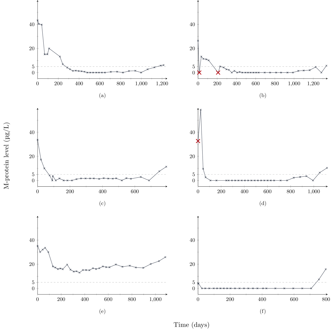
Figure 1: Some examples of trajectories from the dataset. The crosses correspond to observations and the black lines in between are linear interpolations. Trajectories (a) and (c) are kept as-is. Red crosses in trajectories (b) and (d) corresponds to observations that where removed. Trajectories (e) and (f) are completely removed from the dataset.

In this work, we are interested in estimating the relapse time of patients, i.e. the time elapsed between the date of entry into remission and the date of onset of relapse. It is also called the survival time. The main difficulty of the problem lies in the fact that we only have access to partial observations. The M-protein level evolves continuously but is only measured at discrete dates, and so changes in patient condition are never observed. Added to this is the fact that clinical trial data is always fraught with noise.

The raw data has been preprocessed to remove observations unsuitable for model fitting and the procedure is as follows. We start by iteratively removing the first observation of a trajectory if it is lower than the second one to ensure that the beginning of the trajectory corresponds to a phase when the patient is under treatment (see Fig. 1 (d)). We also remove observations with M-protein levels below $1$$\mathrm{\SIUnitSymbolMicro}\mathrm{g}\mathrm{/}\mathrm{L}$ if surrounded by values above $5$$\mathrm{\SIUnitSymbolMicro}\mathrm{g}\mathrm{/}\mathrm{L}$: we assume that these correspond to measurement errors (see Fig. 1 (b)). Then we remove the trajectories whose first observation is lower than a threshold of $5$$\mathrm{\SIUnitSymbolMicro}\mathrm{g}\mathrm{/}\mathrm{L}$, value at which the level is considered negligible (see Fig. 1 (f)) and trajectories with less than two observations below $5$$\mathrm{\SIUnitSymbolMicro}\mathrm{g}\mathrm{/}\mathrm{L}$: we assume that the associated subjects never really reached remission (see Fig. 1 (e)). Finally, we eliminate trajectories with fewer than $10$ observations.

The post-processed dataset consists of $479$ trajectories, with a mean of about $32$ observations per trajectory. The overall M-protein levels range from $0.0$ to $102.1$. The level at first visit time ranges from $5.01$ to $102.1$ with a median of $34.6$. On average, the last visit occurs after $1406$ days of follow-up.

3 A new approach based on iterative regression and survival analysis

In this Section we outline a new approach to estimate relapse time of patients undergoing myeloma treatment from partial and noisy observations. We propose to fit a continuous-time parametric model for the evolution of the biomarker. Our approach contains two main steps:

1. We estimate the date of onset of remission and the date of onset of relapse (if any) with iterative curve fitting based on the parametric model.

2. We perform a survival analysis with the relapse times obtained in the previous step to estimate the parameters of the survival distribution.

We have chosen to model our case study using a very simple piecewise-deterministic Markov process, which we describe below. The choice of such a random model offers us simple temporal granularity and interpretable parametrization.

3.1 PDMPs

Piecewise Deterministic Markov Processes, introduced by Davis in the 80’s, are a general class of stochastic processes including almost all non-diffusion models found in applied probability (Davis, 1984). These continuous-time processes are used to describe deterministic motions punctuated by random jumps, and are therefore particularly well suited to model our problem. We now give a brief introduction to PDMPs in a generic framework.

Let $(X_{t})_{t\geq 0}$ be a PDMP defined on a Borel subset $E\subset\mathbb{R}^{d}$. The trajectories of $(X_{t})_{t\geq 0}$ are determined by the behaviour of the process between jumps, as well as when and where the jumps occur. These aspects are described by a flow $\Phi$, a jump intensity $\lambda$ and a Markov kernel $Q$, respectively. The flow $\Phi\colon E\times\mathbb{R}_{+}\to E$ is a continuous function satisfying the semi-group property: $\forall x\in E,\ \forall t,s\in\mathbb{R}_{+},\ \Phi(x,t+s)=\Phi(\Phi(x,t),s)$. Starting from $x\in E$, $\Phi(x,t)$ gives the position of the process after some time $t$ if no jump has occurred (see Figure 2).

[width=.5]./figures/flow

Figure 2: Starting from $x$ at time $0$, the process follows its flow up to time $t$ and ends up at $\Phi(x,t)$, assuming no jump has occurred. Going on up to time $t+s$ is the same as starting from $\Phi(x,t)$ and following the flow for a time $s$.

The process can jump deterministically or randomly. Deterministic jumps occur when the flow reaches the boundary $\partial E$ of $E$. Given a starting point $x\in E$, this happens after a time $t^{*}(x)=\inf\left\{t>0\colon\Phi(x,t)\in\partial E\right\}$. Random jumps are governed by the jump intensity $\lambda\colon E\to\mathbb{R}_{+}$ — also known as the hazard rate — which is a measurable function such that $\forall x\in E,\ \exists\varepsilon>0\colon\int_{0}^{\varepsilon}\lambda(\Phi(x,s))\mathrm{d}s<\infty$. That is, jumps cannot occur instantaneously (and therefore there cannot be several jumps at the same time). The jump times of a PDMP are obtained by taking the minimum between deterministic jumps and stochastic ones. Given a starting point $x_{0}\in E$, for all $t\in\mathbb{R}_{+}$, the first jump time $T_{1}$ satisfies

$$\mathbb{P}_{X_{0}=x_{0}}(T_{1}>t)=\begin{cases}\mathrm{e}^{-\int_{0}^{t}\lambda(\Phi(x_{0},s))\mathrm{d}s}&\text{if}\quad t<t^{*}(x_{0}),\\ 0&\text{if}\quad t\geq t^{*}(x_{0}).\end{cases}$$ (1)

For both deterministic and random jumps, the new location of the PDMP is drawn from the Markov kernel $Q\colon\bar{E}\times\mathcal{B}(\bar{E})\to E$, where $\mathcal{B}(\bar{E})$ is the set of Borel $\sigma$-fields of $\bar{E}$, the closure of $E$. When the process starts from $x\in\bar{E}$, we have that $\forall A\in\mathcal{B}(\bar{E}),\ Q(x,A)=\mathbb{P}(X_{T_{1}}\in A\mid X_{T_{1}^{-}}=x)$, where $T_{1}^{-}$ denotes the time just before the first jump. The Markov kernel $Q$ satisfies $\mathbb{P}(X_{t}=x\mid X_{t^{-}}=x)=0,\forall t\in\mathbb{R}_{+}$. In other words, each jump must involve a real change of location.

It is common practice to separate the state space $E$ into a hybrid one made up of a discrete component and a continuous one, such that $X_{t}=(m_{t},\zeta_{t})\in E\subset M\times\mathbb{R}^{d}$, where $m_{t}$ corresponds to a discrete mode and $\zeta_{t}$ to a continuous variable. Furthermore, the state space can be specific to each mode: $\forall m\in M,\ E_{m}\subset\mathbb{R}^{d_{m}}$. The mode-specific flow $\Phi_{m}$ is such that $\forall m\in M,\ \Phi_{m}\colon E_{m}\times\mathbb{R}_{+}\to E_{m}$ and $\Phi((m,\zeta),t)=(m,\Phi_{m}(\zeta,t))$.

3.2 Model definition and notations

The PDMP used to model the dynamics of the biomarker is illustrated in Figure 3. At the start of their monitoring patients are administered a treatment, the effect of which is to reduce the M-protein level. If the level falls below a certain fixed threshold $\zeta_{r}\in\mathbb{R}$, the patient is considered to be in remission. In the event of a relapse, the serum level rises again. The horizon $H$ of follow-up is different for each patient. There are three possible modes for the subjects in the study. They can be sick under treatment ($m=-1$), sick without treatment ($m=1$) or in remission ($m=0$) — for simplicity, we assume that the process characteristics in remission mode are the same with or without treatment and do not differentiate the two cases. We therefore have $M=\left\{-1,0,1\right\}$ and $E_{-1}=(\zeta_{r},+\infty)$, $E_{0}=\left\{\zeta_{r}\right\}\times\mathbb{R}_{+}$ and $E_{1}=[\zeta_{r},+\infty)$. In mode $m=0$, a time variable $u\in\mathbb{R}_{+}$ is added to the state space to allow more flexibility in the jump intensity while ensuring the Markov property holds. It represents the time spent in remission mode. Under treatment, the biomarker level decreases exponentially with slope $v_{-1}<0$. During relapse, it increases exponentially with slope $v_{1}>0$. For all $\zeta\in\mathbb{R}$ we have

$$\left\{\begin{aligned} &\Phi_{-1}(\zeta,t)=\zeta\mathrm{e}^{v_{-1}t},\\ &\Phi_{0}((\zeta,u),t)=(\zeta,u+t)=(\zeta_{r},u+t)\\ &\Phi_{1}(\zeta,t)=\zeta\mathrm{e}^{v_{1}t}.\end{aligned}\right.$$ (2)

In mode $m=-1$, a jump to $(m=0,\zeta=\zeta_{r},u=0)$ occurs when the subject reaches the fixed remission threshold $\zeta_{r}$. This is therefore a deterministic jump at the boundary. The first jump time $t_{-1}^{*}(\zeta)$ is the solution of $\Phi_{-1}(\zeta,t)=\zeta_{r}$. That is, $t_{-1}^{*}(\zeta)=\frac{1}{v_{-1}}\mathrm{log}(\frac{\zeta_{r}}{\zeta})$. In mode $m=0$ however, the process may jump randomly to $(m=1,\zeta=\zeta_{r})$ and the jump intensity $\lambda_{0}(u)>0$ is unknown. We choose a Weibull distribution to model it, as is conventionally done in survival analysis to model the hazard rate. The probability density function of the Weibull distribution is given by

$$f(u)=\left(\frac{\alpha}{\beta}\right)\left(\frac{u}{\beta}\right)^{\alpha-1}\mathrm{e}^{-\left(\frac{u}{\beta}\right)^{\alpha}},$$ (3)

for $u>0$ and where $\alpha>0$ is a shape parameter and $\beta>0$ is a scale parameter. The intensity is therefore the hazard function

$$\lambda_{0}(u)=\left(\frac{\alpha}{\beta}\right)\left(\frac{u}{\beta}\right)^{\alpha-1}.$$ (4)

Note that a shape parameter $\alpha<1$ (resp. $\alpha>1$) means that the failure rate decreases (resp. increases) over time. If $\alpha=1$, this rate is constant.

We consider that once the process reaches mode $m=1$, no more jump can occur. In our model, the mode-specific Markov kernels are deterministic. When a jump occurs, the biomarker value does not change; only the mode changes, according to a very simple mechanism: at time $t=0$, the process is always in mode $m=-1$ and switches to mode $m=0$ as described above, then possibly to mode $m=1$ if a relapse occurs.

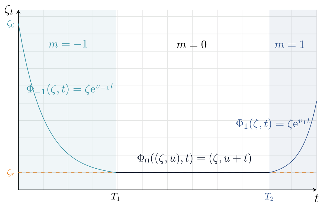
Figure 3: Example trajectory of our PDMP. The PDMP starts in mode $m=-1$ (patient under treatment) from an initial point $\zeta_{0}$ and follows a deterministic trajectory along its exponential flow $\Phi_{-1}$ until the first jump occurs at time $T_{1}$ when reaching the boundary $\zeta=\zeta_{r}$ (remission). The mode switches to $m=0$ and the flow is constant equal to $\zeta_{r}$ until a new jump occurs randomly at time $T_{2}$. The mode switches then to $m=1$ (relapse of the disease) and the trajectory rises exponentially along the flow $\Phi_{1}$.

3.3 Building model estimators

In this section, we explain the estimation procedure for the parameters of our model based on the data. This involves first estimating the process jump times, and then finding the parameters of the relapse time distribution. In what follows, we let $t_{-1}^{*}(\zeta_{0})\coloneqq T_{1}$ be the time of the first jump from mode $m=-1$ to mode $m=0$ and $T_{2}$ the time of the second jump, if any, from mode $m=0$ to mode $m=1$. Note that even though the underlying process is in continuous time, we only have access to observations at discrete visit dates and the estimation procedure must be adapted accordingly. Note that we use regular time intervals between visits for convenience, but that our method remains valid for any intervals. The points do not need to be equally spaced to perform the estimation, as we will see in Section 5.

3.3.1 Jump time estimation

Our estimation method for $T_{1}$ and $T_{2}$ is an iterative optimisation process based on regression. It is described in Algorithm 1. Let $(X_{t})_{t\geq 0}$ be the PDMP defined in Section 3.2 and let $(X_{k})_{k\in\mathbb{N}}=(X_{d_{k}})_{k\in\mathbb{N}}$ be the process at the observation dates $(d_{k})_{k\in\mathbb{N}}$. The observations are defined as $Y_{k}=F(X_{k})\mathrm{e}^{\varepsilon_{k}}$, where $\varepsilon_{k}\sim\mathcal{N}(0,\sigma^{2})$ is a Gaussian noise and where $F\colon E\to\mathbb{R}_{+}$ is a function that returns the marker component of the PDMP. Hence, $Y_{k}=\zeta_{k}\mathrm{e}^{\varepsilon_{k}}$. We use a multiplicative noise both to match the exponential growth and decay of biomarker level and to simplify the estimation procedure described hereafter. We start with the estimation of $T_{1}$.

Fitting the flow to observations For a given $3\leq j\leq N$, let $y_{1:j}=(y_{1},y_{2},\dots,y_{j})$ be the first $j$ values of an $N$-length trajectory of M-protein levels recorded at dates $d_{1},d_{2},\dots d_{j}$, respectively. The biomarker level has an exponential form, so we use least squares to fit a linear function $f\colon x\mapsto ax+b$ to the logarithm of our data, and we let $\widetilde{a}=\widetilde{v_{-1}}$ and $\mathrm{e}^{\widetilde{b}}=\widetilde{\zeta_{0}}$ be the optimal solutions of the problem. We use a logarithmic transformation to prevent errors at the beginning of the trajectory from having too much weight on the overall error.

Computing the fit error We then estimate $T_{1}$ as the solution for $t$ of $\mathrm{e}^{\widetilde{b}}\mathrm{e}^{\widetilde{a}t}=\zeta_{r}$ (see Alg. 1 l. 1). This gives us an approximation $\widetilde{T_{1}}$ of the jump time from $m=-1$ to $m=0$ and we calculate a general regression error $\Delta_{\mathrm{tmp}}$ as the sum of two errors: one between the points falling before $\widetilde{T_{1}}$ and the fitted curve, and the other on the remaining part of the trajectory. That is,

$$\Delta_{\mathrm{tmp}}=\lVert y_{1:k}-\widetilde{b}\mathrm{e}^{-d_{1:k}\times\widetilde{a}}\rVert_{2}^{2}+\lVert y_{k+1:N}-\zeta_{r}\rVert_{2}^{2},$$ (5)

where $k=\lvert\{i;d_{i}\leq\widetilde{T_{1}}\}\rvert$ represents the number of points falling before $\widetilde{T_{1}}$.

Repeating until convergence Note that all the above estimates depend on $j$, which is omitted for clarity. This process is repeated for $j\in\left\{3,\dots,N\right\}$ until a stopping criterion is met, minimizing the error. This results in estimates $\widehat{T_{1}}$ and $\widehat{a}$ for the entry time into remission $T_{1}$ and the slope $v_{-1}$ in mode $m=-1$, respectively. Note that $\widehat{a}$ is only used to estimate $T_{1}$ and will not be used to estimate the relapse time afterwards. Details of the estimation procedure can be found in Algorithm 1. The last condition on line 1 of the algorithm ends the estimation process after $15$ visits if the fitting error stops decreasing to avoid unnecessary iterations.

Estimating the second jump time We can then use the same process again on the remaining part of the trajectory — that is, on $(y_{k})_{\widehat{T_{1}}<k\leq N}$ — to obtain $\widehat{T_{2}}$ and $\widehat{v_{1}}$. It is important to note that if the trajectory is overall very flat, it is not relevant to look for a jump time, plus the algorithmic minimization could fail due to numerical instability. In such cases, we assume that no change in mode occurred. This happens mainly when subjects do not relapse within their follow-up time. They are considered ”censored subjects” and are discussed hereafter.

input : $d\in\mathbb{R}^{N}$ vector of visit dates, $y\in\mathbb{R}^{N}$ vector of observations at visit dates, $\zeta_{r}\in\mathbb{R}$ theoretical threshold for remission mode

1

init: $\Delta=\infty$, $\widehat{T_{1}}=0$, $\widehat{a}=0$, $\widehat{b}=0$

2 for $j=3,\dots,N$ do

    ${d}_{\mathrm{tmp}}=d_{1:j}$ ;

     //slicing of the first $j$ coordinates of $d$

3    ${y}_{\mathrm{tmp}}=y_{1:j}$

4    find $\widetilde{a}$ and $\widetilde{b}$ optimal values when fitting a linearization of $f:x\mapsto a\mathrm{e}^{-bx}$ to $\mathrm{log}({y}_{\mathrm{tmp}})$ using least squares

    $\widetilde{T_{1}}=(\mathrm{log}(\zeta_{r})-\mathrm{log}(\widetilde{b}))/\widetilde{a}$ ;

     //solve $\widetilde{b}\mathrm{e}^{t\widetilde{a}}=\zeta_{r}$ for $t$

5    $k=\lvert\{i;d_{i}\leq\widetilde{T_{1}}\}\rvert$

    $n_{1}=\lVert y_{1:k}-\widetilde{b}\mathrm{e}^{-d_{1:k}\times\widetilde{a}}\rVert_{2}^{2}$ ;

     //error between the first $k$ points and the fitted curve

    $n_{2}=\lVert y_{k+1:N}-\zeta_{r}\rVert_{2}^{2}$ ;

     //error on the remaining part of the trajectory

6    ${\Delta}_{\mathrm{tmp}}=n_{1}+n_{2}$

7    if ${\Delta}_{\mathrm{tmp}}\leq\Delta$ $\mathrm{AND}$ $\widetilde{T_{1}}>0$ then

8       $\Delta={\Delta}_{\mathrm{tmp}}$

9       $\widehat{T_{1}}=\widetilde{T_{1}}$

10       $\widehat{a}=\widetilde{a}$

11       $\widehat{b}=\widetilde{b}$

12      

13   if ${\Delta}_{\mathrm{tmp}}>\Delta$ $\mathrm{AND}$ $\widetilde{T_{1}}>0$ $\mathrm{AND}$ $j>15$ then break;

14   

return $\widehat{T_{1}},\widehat{a},\widehat{b}$

Algorithm 1 Jump time estimation

3.3.2 Survival time before relapse

Having calculated $\widehat{T_{1}}$ and $\widehat{T_{2}}$ for each trajectory, we now have access to the survival times of the subjects, that is, the elapsed time between the start of the remission and the beginning of the relapse, if any, or the follow-up time otherwise. Following the terms of survival analysis, an event is defined as the occurrence of a relapse. A patient is considered censored if no event has occurred until the end of its follow-up. The survival function $S(t)=\mathbb{P}(T_{2}-T_{1}>t)$ gives us the probability that a patient remains in remission beyond a time $t$ after remission entry, and we seek to recover its parameters. To estimate the parameters of the Weibull distribution, we fit a parametric survival regression model with the survival time as a response variable together with a censoring indicator. This gives us the estimations $\widehat{\alpha}$ and $\widehat{\beta}$ of the shape and scale parameters, respectively.

4 Simulation study

We evaluate the performance of our estimation strategy through a simulation study and explore the influence of nuisance parameters on a range of scenarios. We then compare our approach with existing methods for estimating relapse time.

The average computation time for the full estimation process (two-sided trajectory fitting and survival regression) for $500$ samples is $7.2\text{\,}\mathrm{s}$. All codes are executed on a laptop computer with an Intel(R) Core(TM) i$7$-$12700$H processor using $16\text{\,}\mathrm{GB}$ of RAM.

4.1 Generating data

We use Algorithm 2 to simulate trajectories. It simulates a trajectory according to the PDMP model described in Section 3.2, and adds additive noise. The threshold $\zeta_{r}$ for remission mode, the first M-protein level $\zeta_{0}$, the time of last observation $H$, the shape and scale of the Weibull distribution as well as the slopes $v_{-1}$ and $v_{1}$ are all chosen to produce trajectories that are qualitatively similar to those observed in the application dataset presented in Section 2. The nuisance parameters, i.e. the time interval $\delta$ between visits and the level of noise $\sigma$, together with the number $n$ of trajectories in a cohort are studied over three different scenarios.

• The number $n$ of trajectories and the noise level $\sigma$ are fixed while the number of days between visit varies, with $\delta\in\left\{10,20,30,40,50,60\right\}$.

• The number of trajectories $n$ and the visit interval $\delta$ are fixed while the noise level varies, with $\sigma\in\left\{0.25,1,2.5,5\right\}$.

• The noise level $\sigma$ and the visit interval $\delta$ are fixed while the number of trajectories varies, with $n\in\left\{100,500,1000,5000,10000\right\}$.

The parameters used in the simulations for each scenario are summarized in Table 1.

Table 1: Parameters used to simulate trajectories under the three scenarios.

	Scenario i@	Scenario ii@	Scenario iii@
$n$	$500$	$500$	$\left\{250,500,1000,5000,10000\right\}$
$\delta$	$\left\{10,20,30,40,50,60\right\}$	$30$	$30$
$\sigma$	$1$	$\left\{0.25,1,2.5,5\right\}$	$1$
$\zeta_{0}$	$\mathcal{U}_{\left[15,55\right]}$	$\mathcal{U}_{\left[15,55\right]}$	$\mathcal{U}_{\left[15,55\right]}$
$H$	$\mathcal{U}_{\left[900,1900\right]}$	$\mathcal{U}_{\left[900,1900\right]}$	$\mathcal{U}_{\left[900,1900\right]}$
$(\alpha,\beta)$	$(4.69,1650)$	$(4.69,1650)$	$(4.69,1650)$
$v_{-1}$	$-0.046$	$-0.046$	$-0.046$
$\zeta_{r}$	$1$	$1$	$1$
$v_{1}$	$0.012$	$0.012$	$0.012$

input :  $l_{0},u_{0}\in\mathbb{R}$, $l_{H},u_{H}\in\mathbb{R}$, lower and upper bounds for starting point and follow-up time distribution, $\alpha,\beta\in\mathbb{R}$ shape and scale parameters for the Weibull distribution, $v_{-1},v_{1}\in\mathbb{R}$ slopes for mode $m=-1$ and $m=1$, $\delta\in\mathbb{N}$ number of days between two visit dates, $\sigma\in\mathbb{R}^{+}$ standard deviation of the Gaussian noise, $\zeta_{r}\in\mathbb{R}$ theoretical threshold for remission mode

1

init: $\zeta_{0}\sim\mathcal{U}_{\left[l_{0},u_{0}\right]}$, $H\sim\mathcal{U}_{\left[l_{H},u_{H}\right]}$

2

3$T_{1}\leftarrow(\mathrm{log}(\zeta_{r})-\mathrm{log}(\zeta_{0}))/v_{-1}$ ; $w\sim\mathcal{W}(\alpha,\beta)$

$T_{2}\leftarrow T_{1}+w$ ; $c\leftarrow\mathds{1}_{\left\{H\leq T_{2}\right\}}$ ;

  //c censoring indicator

$\delta_{\mathrm{end}}\leftarrow\lfloor H/\delta\rfloor$ ;

  //last visit date

4 for $k=0,\dots,\delta_{\mathrm{end}}$ do

    $d_{k}\leftarrow k\delta$ ;

     //visit dates at regular time intervals until $H$

5    $m_{k}\leftarrow-\mathds{1}_{\left\{d_{k}<T_{1}\right\}}+\mathds{1}_{\left\{d_{k}>T_{2}\right\}}$

6   

7   if $m_{k}=-1$ then

8       $\zeta_{k}\leftarrow\Phi_{-1}(\zeta_{r},d_{k})$ ;

9      

10    else if $m_{k}=0$ then

11       $\zeta_{k}\leftarrow\zeta_{r}$ ;

12      

13    else

14       $\zeta_{k}\leftarrow\Phi_{1}(\zeta_{r},d_{k}-T_{2})$ ;

15      

16   $y_{k}=\zeta_{k}+\mathcal{N}(0,\sigma^{2})$

return $y=(y_{k})_{k}$

Algorithm 2 Simulation of one trajectory from a PDMP

4.2 Evaluation of the method

We present here the most relevant results. The online supplementary material contains all the results for the three scenarios. For each experiment, our method is evaluated on 100 batches of $n$ trajectories to take account of variability.

We evaluate our method by examining the errors made on the estimated parameters, namely $T_{1}$, $T_{2}$, $\alpha$ and $\beta$, as well as on the censoring prediction. Jump time estimates are compared with the true parameters in absolute distance. Weibull parameter estimates are compared with the true parameters in relative distance, since the two are of different orders of magnitude. We do not take into account the distance between distributions, as we use a parametric estimation method.

Scenario i@

Figure 4.2 presents the distributions of absolute errors on the estimates of $T_{1}$ and $T_{2}$ depending on visit frequency. Unsurprisingly, with longer time intervals between visits both the mean error and the variability on $\widehat{T_{1}}$ increase, as fewer points are available to fit the trajectory. For $\widehat{T_{2}}$ on the other hand, the evolution of error and variability with $\delta$ is less obvious. Note that the errors shown in the figure only concern trajectories for which a relapse has occurred and been correctly detected. We can thus assume that these are more obvious relapses, and therefore relapses for which $T_{2}$ is easier to estimate. For $\delta=50$ and $\delta=60$, the average number of days of error on the first jump time is close to the time interval itself: the estimate $\widehat{T_{1}}$ is on average one visit apart from the actual jump time $T_{1}$. For $\delta\leq 40$ however, the error on $\widehat{T_{1}}$ is about half the value of the time interval. For $\delta\leq 20$, the mean error on $\widehat{T_{1}}$ is less that the one on $\widehat{T_{2}}$, whereas the opposite occurs for larger values of $\delta$. Absolute errors on overall relapse times $T_{2}-T_{1}$ are available in Table LABEL:supp-tab:survivalerrorscenario1 of the supplementary materials. Average survival time for patients who relapse is around $1100$ days, hence errors on these durations are relatively small.

Figure 4.2 shows the distributions of relative errors on Weibull shape and scale parameter estimates. The average error on the shape parameter $\alpha$ increases with the time between visits. This is fairly consistent with the results in Figure 4.2, since increasing $\delta$ degrades the estimate of both jump times and therefore spreads out the distribution of relapse time. The average relative error on $\widehat{\beta}$ remains constant as the time between visits increases. Figure 4.2 shows the empirical distribution of relapse times for $\delta=30$, together with the Weibull probability density function with shape and scale parameters fitted on the trajectories and the ground-truth density. The estimated distribution has a slightly higher mode than the true one and is more spread out. Note however that with $\delta=30$, a batch of trajectories contains on average $66.7\%$ of censored cases so our method is inevitably biased. This aspect will be developed further below. The same curves for other values of $\delta$ are shown in Figure LABEL:supp-fig:pdfsscenario1 of the supplementary materials. Figure 4.2 represents the average confusion matrix from the estimation on $100$ batches of trajectories with $\delta=30$. A false censoring occurs when the $T_{2}$ estimates falls after the time horizon $H$. Such errors tend to appear more often as the time interval between visits increases (see Figure LABEL:supp-fig:confusiontablesscenario1 in supplementary materials): the longer we wait before checking a patient again, the more likely we are to miss a relapse. Our estimation procedure almost never predicts a relapse when there is none. This is the case for all the visit intervals considered (see supplementary materials). This result can be strongly influenced by the noise level in the trajectories, as illustrated in Scenario ii@.

Boxplots of absolute number of days of error on estimated jump times $\widehat{T_{1}}$ and $\widehat{T_{2}}$ on one batch with $n=500$ trajectory samples, depending on the visit interval $\delta$ (in days). Errors on both parameters are only calculated on trajectories for which relapse occurred and is correctly predicted. [.45]  Boxplots of relative error on Weibull shape and scale parameter estimates over $100$ batches with $n=500$ trajectory samples, depending on the visit interval $\delta$ (in days). [.45]

Distribution of relapse times fitted on one batch of $n=500$ trajectory samples, for $\delta=30$. The plain curve represents the Weibull probability density function with shape and scale parameters fitted on the trajectory batch. The dashed curve shows the ground-truth density. Times are only shown for trajectories for which relapse occurred and is correctly predicted. [.45]  Confusion table from the estimation process repeated over $100$ batches, for $\delta=30$. Values are rounded to the nearest $10^{-2}$. [.45]

Scenario ii@

Figure 4 shows the confusion matrices obtained for different noise levels. The noisier the trajectory, the more difficult it is to detect true relapses. This is also illustrated in Figure 4.2, where we see a deterioration in the $T_{2}$ estimate as $\sigma$ increases. Figure 4.2 suggests that the estimation errors on jump times have a direct impact on the estimation of the shape parameter $\alpha$ of the relapse time distribution. On the other hand, these errors do not seem to affect the estimation of $\beta$. Overall, the increase in noise level only slightly alters the estimates. Note that for $\sigma=2.5$ and $\sigma=5$, the noise level is much higher than that likely to be found in the trajectories of the application dataset. This scenario shows that the limitation of our estimation method does not stems from the amount of noise in the data.

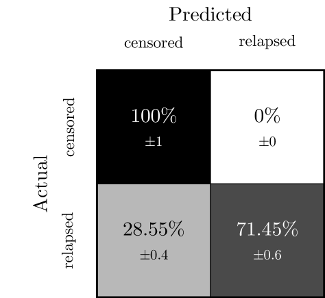
(a) $n=500,\delta=30,\sigma=0.25$

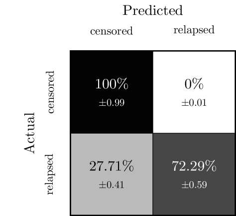
(b) $n=500,\delta=30,\sigma=1.0$

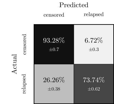
(c) $n=500,\delta=30,\sigma=2.5$

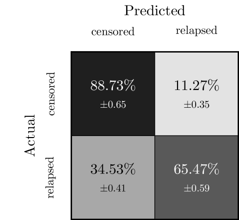
(d) $n=500,\delta=30,\sigma=5.0$

Figure 4: Confusion tables from the estimation process repeated over $100$ batches, depending on noise level $\sigma$.

Boxplots of absolute number of days of error on estimated jump times $\widehat{T_{1}}$ and $\widehat{T_{2}}$ on one batch with $n=500$ trajectory samples, depending on noise level $\sigma$. Errors are only calculated on trajectories for which relapse occurred and is correctly predicted. [.45]  Boxplots of relative error on Weibull shape and scale parameter estimates over $100$ batches with $n=500$ trajectory samples, depending on noise level $\sigma$. [.45]

Scenario iii@

Increasing the sample size can be expected to have no impact on the quality of the estimates, and this is borne out in practice (see Supplementary materials, Scenario iii@). We can nevertheless verify on Figure 5 that the variance of the estimates of the parameters of the survival time distribution decreases with the size of the cohort, as expected.

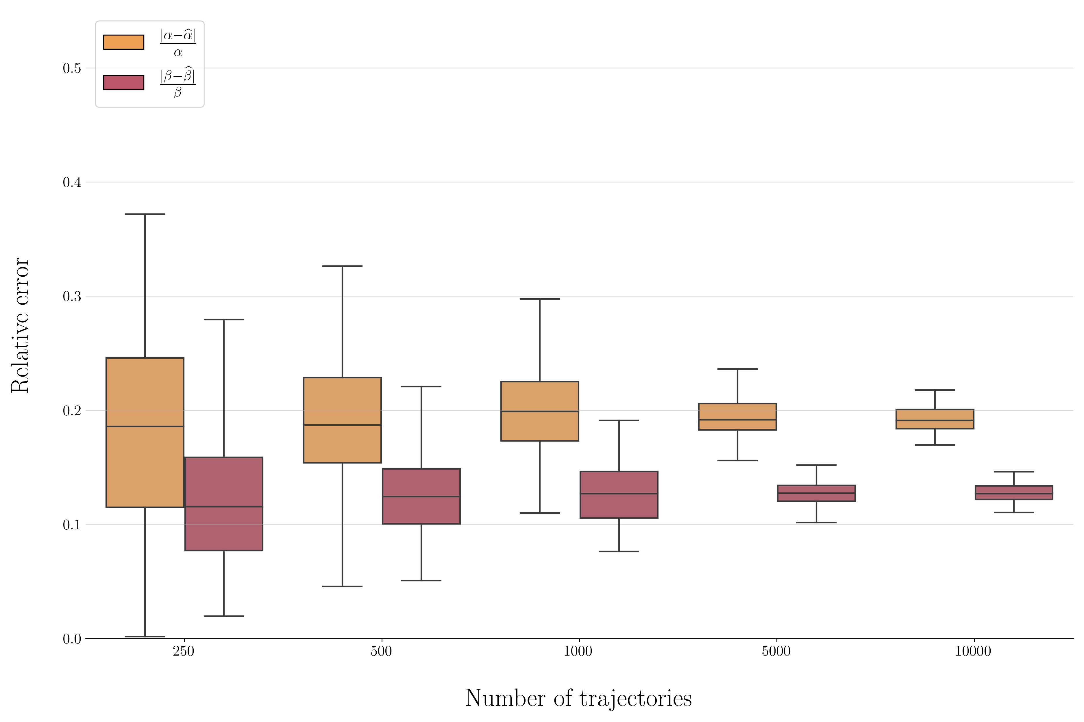
Figure 5: Boxplots of relative error on Weibull shape and scale parameter estimates over $100$ batches, depending on the number $n$ of trajectories.

Discussion on the simulation study

As already mentioned, our method has an intrinsic bias due to the presence of censoring. We tend to overestimate relapse times, whatever the visit interval or noise level. Further experiments confirm that removing the estimation error on both jump times does alleviate the problem (see Figure LABEL:supp-fig:noesterr in the Supplementary material). Increasing the follow-up time could improve the estimation of the second jump time, and therefore estimation of the overall the relapse time but we have chosen not to perform such experiment, as this approach would not be realistic for our application case. Reducing the estimation error of relapse times in the presence of censoring remains an open question.

All the trajectories associated with the results presented here were simulated with the same pair $(\alpha,\beta)$. The same study was carried out with different values of these parameters and the results are available in Section LABEL:supp-sec:scenariosa of the Supplementary materials.

4.3 Comparison with other methods

We now compare our estimation method with change point detection and Hidden Markov Models (HMMs). Both methods exploit little or no information about the model, which is one of their advantages. But we choose to give them as much model knowledge as possible to improve their performance. We develop the estimation procedure with change point detection and HMMs, and explain how we compare them with our method.

4.3.1 Change point detection

Given a non-stationary signal $y$, (offline) change point detection aims to find the best segmentation of $y$ into a piecewise stationary signal by detecting when the signal changes dynamics. This is done by minimizing some predefined criterion.

The signal considered is the logarithm of the consecutive differences of the simulated trajectories. That is, if $(y_{i})_{i=1,\ldots,N}$ is an $N$-length trajectory, the signal is $(\mathrm{log}(y_{i})-\mathrm{log}(y_{i+1}))_{i=1,\ldots,N-1}$. We focus on trajectories where a relapse occurs and therefore set the number $K$ of breakpoints to be detected at $K=2$. This allows us to recover the $3$ modes of the process. We assume that our signal is Gaussian, with piecewise constant mean and fixed variance. We thus use a quadratic error loss as criterion function, a common practice in such cases.

Change point detection is implemented using the ruptures python library (Truong et al., 2020).

4.3.2 HMMs

Here our trajectories are seen as a sequence of observations linked to hidden states of an underlying Markov process. We use an HMM to recover these hidden states, which correspond to the modes of the trajectories. An HMM is determined by the transition probabilities between states, the parameters of the emission probability distributions and the initial state distribution. Given the observations, we seek to estimate the model parameters and infer the hidden states.

Again, the sequence of observations is the logarithm of consecutive differences from the trajectories. We use model information to initialize and constrain some of the model parameters. First, as with change point detection we only consider trajectories where a relapse truly occurs and fix the number of hidden states to $3$. Then, we initiate the initial state distribution so that the probability of starting in mode $m=-1$ is $1$, according to our simulation procedure. The initial transition probability matrix $\mathbf{A}$ is given in Equation (6). For example, given that the process is currently in mode $m=-1$, the probability of switching to mode $m=0$ is initiated to $0.7$, hence higher than staying in mode $m=0$. This broadly reflects the behaviour of the trajectories. Finally, we constrain the transition matrix to prevent impossible transitions and fix the absorbing state. Denoting $m_{t}$ the mode at time $t$, the transition matrix is such that $\mathbb{P}(m_{t}=-1\mid m_{t-1}=0)=\mathbb{P}(m_{t}=-1\mid m_{t-1}=1)=0$, $\mathbb{P}(m_{t}=0\mid m_{t-1}=1)=0$, $\mathbb{P}(m_{t}=1\mid m_{t-1}=-1)=0$ and $\mathbb{P}(m_{t}=1\mid m_{t-1}=1)=1$:

$$\mathbf{A}=\blockarray{cccr}{\color[rgb]{0,0,0}-1}&{\color[rgb]{0,0,0}0}&{\color[rgb]{0,0,0}1}\\ \block{(ccc)r}0.3&0.7&0.0&{\color[rgb]{0,0,0}-1}\\ 0.0&0.4&0.6&{\color[rgb]{0,0,0}0}\\ 0.0&0.0&1.0&{\color[rgb]{0,0,0}1}\\$$ (6)

The model parameters are then estimated using an adapted version of the hmmlearn python package (Weiss et al., 2024).

4.3.3 Performance comparison

We tried to let both methods deduce the number of modes using common model selection heuristics, but the results were very poor and could not be used for partition comparison. As mentioned before, we therefore only consider trajectories with a relapse, and do not perform survival analysis to recover the parameters of the relapse time distribution. We compare the estimation methods solely on the basis of the mode partitioning of the observations. This is explained below.

Given a trajectory, our estimation method provides two jump times $\widehat{T_{1}}$ and $\widehat{T_{2}}$, which are used to partition observations into three sequences between which the mode changes. The same is done with the breakpoints obtained with the change point detection method. Inferring the hidden states of the HMM gives us a sequence of the same nature. For each trajectory, we therefore have three partitions which we compare using the Adjusted Rand Index.

The Rand Index (RI) (Rand, 1971) is a measure of similarity between two partitions of a set. Given two partitions, the RI is the proportion of pairs of elements that are grouped together or separated together. An RI of $0$ indicated that the two partitions disagree on every single pair while two partitions that have perfectly matching clusters will have an RI of $1$. The Adjusted Rand Index (ARI) is an RI corrected for chance. It ranges from $-0.5$ (total disagreement) to $1$ (perfect agreement) and ensures that random labelling have a score close to $0$. It is more robust than the RI and is the metric we use to compare the methods. Figure LABEL:supp-fig:rs of the supplementary materials presents the RI scores.

We simulate a batch of trajectories with $\delta=30$ and $\sigma=1$. We keep only those with a real relapse and apply each of the three methods. We then calculate the Adjusted Rand Index with the ground truth. The results are shown in Figure 6. With our method, the ARI is close to $1$ and higher than for the other two methods, and the variability is lower. Our method outperforms the other two in terms of ARI.

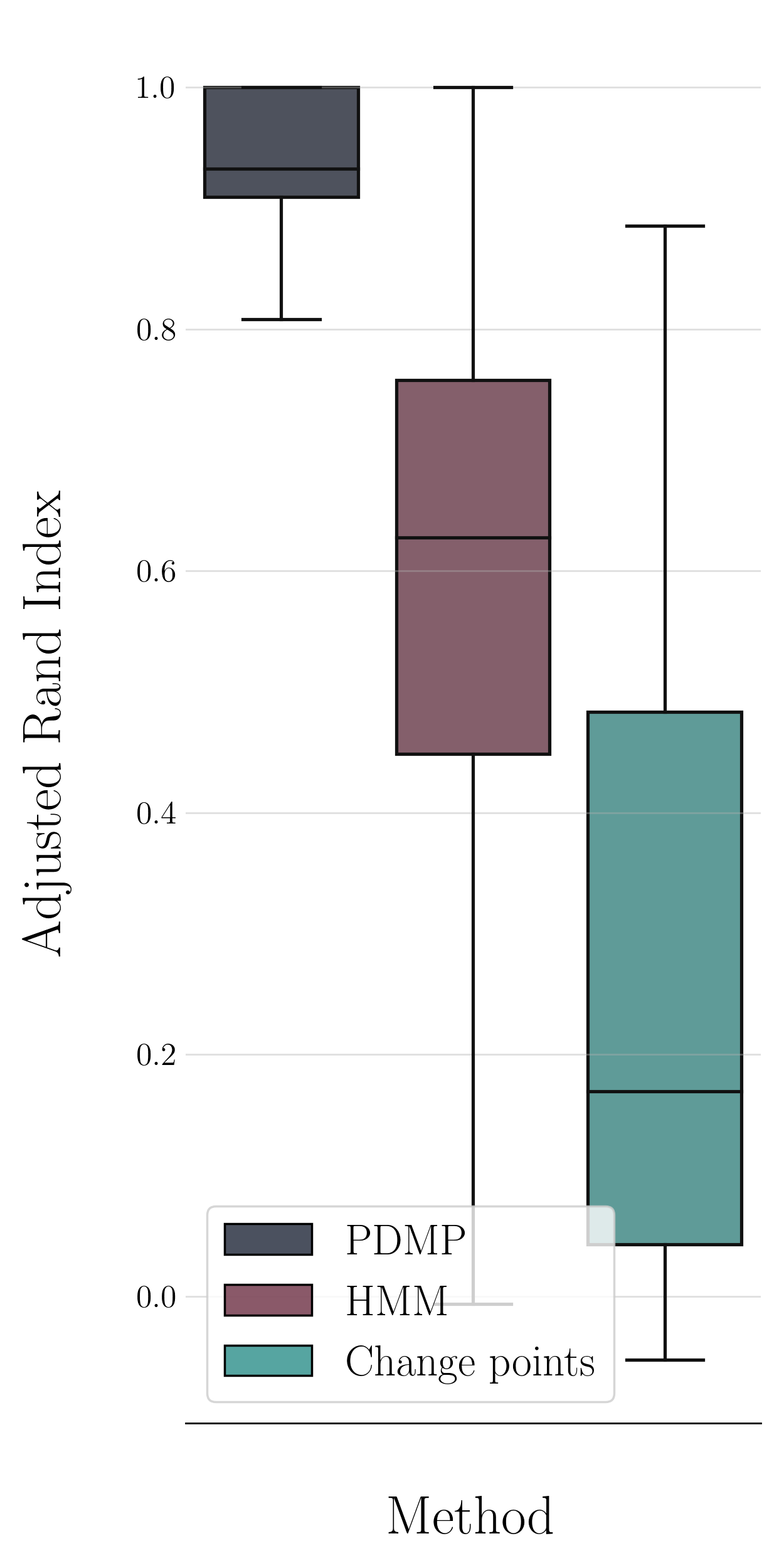
Figure 6: Boxplots of Adjusted Rand Index for the partition into modes depending on the estimation method. The estimation process is applied on one batch of $n=126$ trajectories with relapse, with $\delta=30$ and $\sigma=1.0$.

5 Application to myeloma

The proposed estimation method is applied to the data of interest. The number of trajectories is $479$, as mentioned in Section 2. The survival regression performed with estimated relapse times gives $\widehat{\alpha}=1.1$ and $\widehat{\beta}=2728$. Unsurprisingly, the estimation gives a failure rate that decreases over time. The trajectories from the dataset presented in Figure 1 are shown in Figure 7 with the parameters obtained by the estimation procedure. Note that in our simulation study, we used regular time intervals and similar $\widehat{v_{-1}}$ and $\widehat{v_{1}}$ slopes between patients for simplicity, but our method does not rely on these assumptions. In real data, visits are not equally spaced and the method still works.

Note that the values obtained for $\widehat{\alpha}$ and $\widehat{\beta}$ are quite different from the ones used in the simulation study, but as mentioned in Section 4, the same study was carried out with values of these parameters closer to those from the application and the results are available in Section LABEL:supp-sec:scenariosa of the Supplementary materials.

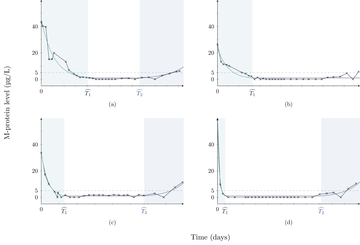
Figure 7: Some examples of trajectories from the dataset. The crosses correspond to observations and the black lines in between are interpolations. The estimated states of the patient are represented by the highlighted areas. The patient is considered in mode $m=-1$ between time $t=0$ and $t=\widehat{T_{1}}$, in mode $m=0$ between $t=\widehat{T_{1}}$ and $t=\widehat{T_{2}}$, and in mode $m=1$ after $t=\widehat{T_{2}}$. The estimated flow is represented by the curve with the corresponding colours.

6 Discussion and conclusion

We proposed a parametric continuous-time model which allows to model the progression of myeloma disease in a cohort of patients. The interest of our method lies in the fact that we estimate not only the time to relapse, but also the time to entry into remission, enabling us to understand and estimate the distribution of time spent in remission. This is a different approach from that generally adopted by survival analysis or online-based prediction methods. These reconstructed durations can then be used by other models for further analysis, especially for non-parametric estimation and methods using covariates. One limitation of our method is that it does not apply online. It requires the entire trajectory to have already been observed, and therefore cannot be plugged into a decision protocol as such. Our method is illustrated on a very simple type of trajectory, but it can easily be extended to more complex dynamics. In particular, it is not limited to exponential flow trajectories, nor to dimension 1, and can be adapted to detect more than two jumps.

7 Data availability and code

The data presented in this article and the code used to reproduce the results and the figures are available at https://github.com/AmelieVernay/pdmp_relapse_time.

8 Fundings

We acknowledge the support of European Union’s Horizon 2020 research and innovation program (https://marie-sklodowska-curie-actions.ec.europa.eu, Marie Sklodowska-Curie grant agreement No 890462, to Alice Cleynen), and of the French National Research Agency (ANR), under grant ANR-20-CHIA-0001 (https://anr.fr/, project CAMELOT, to Amélie Vernay). We also acknowledge the ANR under grant ANR-21-CE40-0005 (https://anr.fr/, project HSMM-INCA).

Bibliography

- Amoros et al. (2019) Ruben Amoros, Ruth King, Hidenori Toyoda, Takashi Kumada, Philip J. Johnson, and Thomas G. Bird. A continuous-time hidden Markov model for cancer surveillance using serum biomarkers with application to hepatocellular carcinoma. METRON, 77(2):67–86, August 2019. doi: 10.1007/s40300-019-00151-. URL https://ideas.repec.org/a/spr/metron/v77y2019i2d10.1007_s40300-019-00151-8.html.
- Attal et al. (2017) Michel Attal, Valerie Lauwers-Cances, Cyrille Hulin, Xavier Leleu, Denis Caillot, Martine Escoffre, Bertrand Arnulf, Margaret Macro, Karim Belhadj, Laurent Garderet, et al. Lenalidomide, bortezomib, and dexamethasone with transplantation for myeloma. New England Journal of Medicine, 376(14):1311–1320, 2017.
- Azaïs and Bouguet (2018) Romain Azaïs and Florian Bouguet, editors. Statistical Inference for Piecewise‐deterministic Markov Processes. Wiley, 1 edition, 2018. ISBN 978-1-78630-302-8 978-1-119-50733-8. doi: 10.1002/9781119507338. URL https://onlinelibrary.wiley.com/doi/book/10.1002/9781119507338.
- Azaïs et al. (2014) Romain Azaïs, François Dufour, and Anne Gégout‐Petit. Non‐Parametric Estimation of the Conditional Distribution of the Interjumping Times for Piecewise‐Deterministic Markov Processes. Scandinavian Journal of Statistics, 41(4):950–969, 2014. ISSN 0303-6898, 1467-9469. doi: 10.1111/sjos.12076. URL https://onlinelibrary.wiley.com/doi/10.1111/sjos.12076.
- Bartolomeo et al. (2011) Nicola Bartolomeo, Paolo Trerotoli, and Gabriella Serio. Progression of liver cirrhosis to hcc: an application of hidden markov model. BMC Medical Research Methodology, 11(1):38, Apr 2011. ISSN 1471-2288. doi: 10.1186/1471-2288-11-38. URL https://doi.org/10.1186/1471-2288-11-38.
- Davis (1984) MHA. Davis. Piecewise-deterministic Markov processes: a general class of nondiffusion stochastic models. J. Roy. Statist. Soc. Ser. B, 46(3):353–388, 1984. With discussion.
- Drescher et al. (2013) Charles W. Drescher, Chirag Shah, Jason Thorpe, Kathy O’Briant, Garnet L. Anderson, Christine D. Berg, Nicole Urban, and Martin W. McIntosh. Longitudinal screening algorithm that incorporates change over time in ca125 levels identifies ovarian cancer earlier than a single-threshold rule. Journal of Clinical Oncology, 31(3):387–392, 2013. doi: 10.1200/JCO.2012.43.6691. URL https://ascopubs.org/doi/abs/10.1200/JCO.2012.43.6691. PMID: 23248253.
- Fonteijn et al. (2012) Hubert M. Fonteijn, Marc Modat, Matthew J. Clarkson, Josephine Barnes, Manja Lehmann, Nicola Z. Hobbs, Rachael I. Scahill, Sarah J. Tabrizi, Sebastien Ourselin, Nick C. Fox, and Daniel C. Alexander. An event-based model for disease progression and its application in familial alzheimer’s disease and huntington’s disease. NeuroImage, 60(3):1880–1889, 2012. ISSN 1053-8119. doi: https://doi.org/10.1016/j.neuroimage.2012.01.062. URL https://www.sciencedirect.com/science/article/pii/S1053811912000791.
- Han et al. (2020) Yongli Han, Paul S. Albert, Christine D. Berg, Nicolas Wentzensen, Hormuzd A. Katki, and Danping Liu. Statistical approaches using longitudinal biomarkers for disease early detection: A comparison of methodologies. Statistics in Medicine, 39(29):4405–4420, 2020. doi: https://doi.org/10.1002/sim.8731. URL https://onlinelibrary.wiley.com/doi/abs/10.1002/sim.8731.
- Krell (2016) Nathalie Krell. Statistical estimation of jump rates for a piecewise deterministic Markov processes with deterministic increasing motion and jump mechanism. ESAIM: Probability and Statistics, 20:196–216, 2016. ISSN 1292-8100, 1262-3318. doi: 10.1051/ps/2016013. URL http://www.esaim-ps.org/10.1051/ps/2016013.
- Krell and Schmisser (2021) Nathalie Krell and Émeline Schmisser. Nonparametric estimation of jump rates for a specific class of piecewise deterministic Markov processes. Bernoulli, 27(4), 2021. ISSN 1350-7265. doi: 10.3150/20-BEJ1312. URL https://projecteuclid.org/journals/bernoulli/volume-27/issue-4/Nonparametric-estimation-of-jump-rates-for-a-specific-class-of/10.3150/20-BEJ1312.full.
- Lorenzi et al. (2019) Marco Lorenzi, Maurizio Filippone, Giovanni B. Frisoni, Daniel C. Alexander, and Sebastien Ourselin. Probabilistic disease progression modeling to characterize diagnostic uncertainty: Application to staging and prediction in alzheimer’s disease. NeuroImage, 190:56–68, 2019. ISSN 1053-8119. doi: https://doi.org/10.1016/j.neuroimage.2017.08.059. URL https://www.sciencedirect.com/science/article/pii/S1053811917307061. Mapping diseased brains.
- Rand (1971) William M. Rand. Objective criteria for the evaluation of clustering methods. Journal of the American Statistical Association, 66(336):846–850, 1971. ISSN 01621459, 1537274X. URL http://www.jstor.org/stable/2284239.
- Severson et al. (2020) Kristen A. Severson, Lana M. Chahine, Luba Smolensky, Kenney Ng, Jianying Hu, and Soumya Ghosh. Personalized input-output hidden markov models for disease progression modeling. In Finale Doshi-Velez, Jim Fackler, Ken Jung, David Kale, Rajesh Ranganath, Byron Wallace, and Jenna Wiens, editors, Proceedings of the 5th Machine Learning for Healthcare Conference, volume 126 of Proceedings of Machine Learning Research, pages 309–330. PMLR, 07–08 Aug 2020. URL https://proceedings.mlr.press/v126/severson20a.html.
- Tang et al. (2017) Xiaoying Tang, Michael I. Miller, and Laurent Younes. Biomarker change-point estimation with right censoring in longitudinal studies. The Annals of Applied Statistics, 11(3):1738 – 1762, 2017. doi: 10.1214/17-AOAS1056. URL https://doi.org/10.1214/17-AOAS1056.
- Truong et al. (2020) Charles Truong, Laurent Oudre, and Nicolas Vayatis. Selective review of offline change point detection methods. Signal Processing, 167:107299, 2020. ISSN 0165-1684. doi: https://doi.org/10.1016/j.sigpro.2019.107299. URL https://www.sciencedirect.com/science/article/pii/S0165168419303494.
- van Delft et al. (2022) Frederik A. van Delft, Milou Schuurbiers, Mirte Muller, Sjaak A. Burgers, Huub H. van Rossum, Maarten J. IJzerman, Hendrik Koffijberg, and Michel M. van den Heuvel. Modeling strategies to analyse longitudinal biomarker data: An illustration on predicting immunotherapy non-response in non-small cell lung cancer. Heliyon, 8(10):e10932, 2022. ISSN 2405-8440. doi: https://doi.org/10.1016/j.heliyon.2022.e10932. URL https://www.sciencedirect.com/science/article/pii/S2405844022022204.
- Weiss et al. (2024) Ron Weiss, Shiqiao Du, Jaques Grobler, David Cournapeau, Fabian Pedregosa, Gael Varoquaux, Andreas Mueller, Bertrand Thirion, Daniel Nouri, Gilles Louppe, Jake Vanderplas, John Benediktsson, Lars Buitinck, Mikhail Korobov, Robert McGibbon, Stefano Lattarini, Vlad Niculae, csytracy, Alexandre Gramfort, Sergei Lebedev, Daniela Huppenkothen, Christopher Farrow, Alexandr Yanenko, Antony Lee, Matthew Danielson, and Alex Rockhill. hmmlearn, 2024. URL https://github.com/hmmlearn/hmmlearn.