Direct estimation of arbitrary observables of an oscillator

Abstract

Quantum harmonic oscillators serve as fundamental building blocks for quantum information processing, particularly within the bosonic circuit quantum electrodynamics (cQED) platform. Conventional methods for extracting oscillator properties rely on predefined analytical gate sequences to access a restricted set of observables or resource-intensive tomography processes. Here, we introduce the Optimized Routine for Estimation of any Observable (OREO), a numerically optimized protocol that maps the expectation value of arbitrary oscillator observables onto a transmon state for efficient single-shot measurement. We demonstrate OREO in a bosonic cQED system as a means to efficiently measure phase-space quadratures and their higher moments, directly obtain faithful non-Gaussianity ranks, and effectively achieve state preparation independent of initial conditions in the oscillator. These results position OREO as a powerful and flexible tool for extracting information from quantum harmonic oscillators, unlocking new possibilities for measurement, control, and state preparation in continuous-variable quantum information processing.

Quantum harmonic oscillators offer a powerful framework for generating and manipulating photons, which are fundamental resources for a wide range of quantum information processing applications [1]. Amongst various physical implementations, the bosonic cQED platform, which leverages superconducting microwave cavities coupled to nonlinear ancillary transmon qubit, stands out for its excellent quantum coherence and control versatility [2, 3]. Thanks to these features, bosonic cQED systems have enabled many remarkable achievements, from the creation of robust logical qubits [4, 5, 6] to the demonstrations of effective quantum metrology [7, 8].

In typical bosonic cQED devices, information about the harmonic oscillator is extracted via a controlled unitary operation that maps a target property of the oscillator to a distinct transmon state. Three main analytical gate sequences have been developed to enable direct experimental access to the expectation values of the excitation number [9], parity [10], and displacement [11] operators. Each of these affords a path towards full tomography [12, 13], which then allows experimenters to extract any target information from the reconstructed oscillator state via post-processing. However, such tomographic approaches are typically resource intensive and often excessive when the desired information is associated with a specific observable. Thus, it is desirable to explore a more versatile experimental procedure capable of directly mapping the expectation value of an arbitrary target observable to a transmon state which is then efficiently extracted via a single observable measurement.

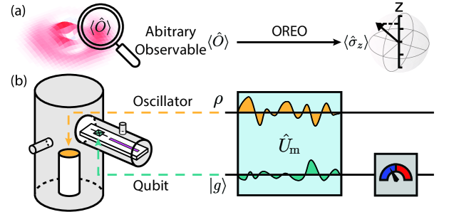
Figure 1: Observable mapping. (a) The Optimize Routine for Estimation of any Observable (OREO) maps the expected value of any target observable $\langle\hat{O}\rangle$ of a harmonic oscillator state onto the z-axis of a qubit’s Bloch vector. (b) Archetypal cQED setup used to demonstrate the technique. The protocol consists of a numerically optimized pulse $\hat{U}_{\text{m}}$ applied to the oscillator-qubit system, followed by a qubit measurement. The expectation value $\langle\hat{O}\rangle$ is obtained from post-processing of $\langle\hat{\sigma}_{z}\rangle$ obtained from standard single-shot qubit readout.

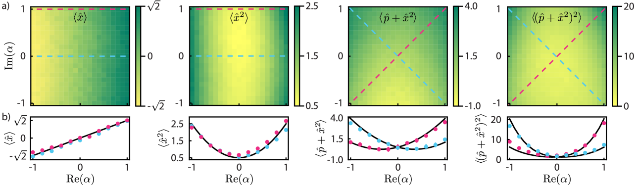
Figure 2: Direct estimation of polynomials of phase-space quadratures. a) Application of OREO to directly obtain the values of $\langle\hat{x}\rangle$, $\langle\hat{x}^{2}\rangle$, $\langle\hat{p}+\hat{x}^{2}\rangle$, and $\langle(\hat{p}+\hat{x}^{2})^{2}\rangle$ of a variable coherent state $|\alpha\rangle$. The dashed lines indicate one-dimensional cuts in the data plotted in (b), which quantitatively agree with the theoretical expected values (solid curves).

In this work, we present a one-fits-all technique to map the expectation value of any observable of a harmonic oscillator to a distinct transmon state detectable via a single-shot measurement. This method, dubbed the Optimized Routine for Estimation of any Observable (OREO), employs numerically optimized pulses to encode the expectation value of a target observable into the state of an auxiliary qubit, allowing oscillator properties to be extracted through standard qubit readout (Fig. 1). This technique is implementable on any oscillator-qubit system that is universally controllable. Here, we experimentally execute OREO in a bosonic cQED architecture where a superconducting cavity dispersively couples to a transmon qubit enabling efficient measurement of several useful observables that are typically inaccessible directly. In the first experiment, we probe the phase space quadratures and their higher-order moments, bridging a common gap in bosonic cQED systems, where direct quadrature measurement is typically hindered by the stationary nature of the oscillator mode. In the second, we apply OREO to quantify degrees of non-Gaussianity, providing an efficient means to assess quantum resources. The last experiment expands on our technique by using the qubit to herald the projection of the oscillator onto an arbitrary state, which affords a strategy to perform robust state preparation independent of the initial condition of the oscillator. These results establish OREO as a versatile and effective tool for extracting information from oscillator states, broadening the capabilities of continuous-variable quantum information processing.

Our implementation of OREO employs a standard bosonic cQED device [14], shown in Fig. 1, in which a three-dimensional superconducting cavity couples to a transmon qubit in the dispersive regime [15]. A planar resonator patterned on the same transmon chip allows direct single-shot measurement of the transmon state. In such a system, universal control of the oscillator state has been demonstrated using numerically optimized drives on both the cavity and transmon [16, 17]. Here, we expand the capabilities of this approach to realize direct mapping of the expectation value of any observable of the bosonic mode to the transmon state.

Conceptually, any observable associated with a quantum harmonic oscillator can be written as $\hat{\mathcal{O}}=\sum_{k}\Lambda_{k}|\psi_{k}\rangle\langle\psi_{k}|$, where $\Lambda_{k}\in\mathbb{R}$ is any real number, and $\{|\psi_{k}\rangle\}$ is any basis. Since the qubit measurement restricts the outcomes to be $\langle\hat{\sigma}_{z}\rangle\in[-1,1]$, we define a scaled version of the observable, $\hat{O}=\hat{\mathcal{O}}/f=\sum_{k}\lambda_{k}|\psi_{k}\rangle\langle\psi_{k}|$ with $f=\max_{k}|\Lambda_{k}|$ such that $\lambda_{k}\in[-1,1]$. Next, we numerically optimize a pulse sequence to enact a unitary operation, $\hat{U}_{\text{m}}$, which is applied to the initial state $|g\rangle\langle g|\otimes\rho$, where $|g\rangle$ is the ground state of the qubit and $\rho$ is an arbitrary state of the oscillator, to implement the mapping process. More specifically, our framework optimizes the drives to satisfy the condition $2\langle g|\hat{U}_{\text{m}}^{\dagger}|g\rangle\langle g|\hat{U}_{\text{m}}|g\rangle-\mathbb{I}_{\text{c}}=\hat{O}$, where $\mathbb{I}_{\text{c}}$ is the identity operator, within a chosen truncation dimension $D$ where the oscillator state is fully contained. This more targeted procedure makes the optimization process computationally efficient, while still preserving its universality [15]. Finally, a standard readout is performed on the qubit after $\hat{U}_{\text{m}}$ to obtain

$$\langle\hat{\sigma}_{z}\rangle = 2p_{g}-1$$ (1)

$$= \text{tr}_{\text{c}}((2\langle g|\hat{U}_{\text{m}}^{\dagger}|g\rangle\langle g|\hat{U}_{\text{m}}|g\rangle-\mathbb{I}_{\text{c}})\rho),$$

where $\hat{\sigma}_{z}$ denotes the Pauli-$z$ operator, $p_{g}$ the probability of the qubit in its ground state, $\text{tr}_{\text{c}}$ the trace with respect to the oscillator. This completes the full OREO process and leads to a direct reading of an abitrary $\langle\hat{O}\rangle$ from the qubit measurement.

To demonstrate the efficacy of OREO in a practical use case, we apply the procedure to directly obtain the expectation values of the phase-space quadratures of the oscillator states residing in the superconducting cavity, as well as their higher moments. Phase-space quadratures are directly accessed in optical systems through homodyne detection and are frequently featured in continuous-variable information processing protocols, such as quantum teleportation, cryptography, and error correction [1]. In contrast, the oscillator states encoded in the stationary modes of superconducting cavities are strongly isolated from the environment, a feature that affords excellent coherence properties but hinders direct access to information about the quadratures. OREO bridges this gap, providing an efficient and practical method to extract the values of quadrature moments of arbitrary order without special hardware requirements. Access to such information provides a valuable primitive for tasks such as the construction of entanglement witnesses [18] and implementations of nonlinear phase gates for universal quantum computation via nonlinear squeezing [19].

Experimentally, we simply probe the excited-state population $p_{e}$ after applying drives obtained numerically to map the quadratures and their higher moments onto the qubit. The measured $p_{e}$ is averaged and corrected for qubit assignment errors, rescaling the result to the $[0,1]$ range [15]. The results for the observables $\langle\hat{x}\rangle$, $\langle\hat{x}^{2}\rangle$, $\langle\hat{p}+\hat{x}^{2}\rangle$ and $\langle(\hat{p}+\hat{x}^{2})^{2}\rangle$ for a coherent state $|\alpha\rangle$ displaced to various locations in phase space are shown in Fig. 2. The data show a strong quantitative agreement with the theoretically predicted outcomes, which confirms that OREO is capable of accurately measuring arbitrary quadrature functions over a wide span of the phase space. Some deviations are observed for larger displacements, for example $|\alpha|\approx\sqrt{2}$. This is due to the leakage of the Fock state population out of the truncation dimension of $D=6$ used in this experiment and can be improved by increasing the truncation dimension.

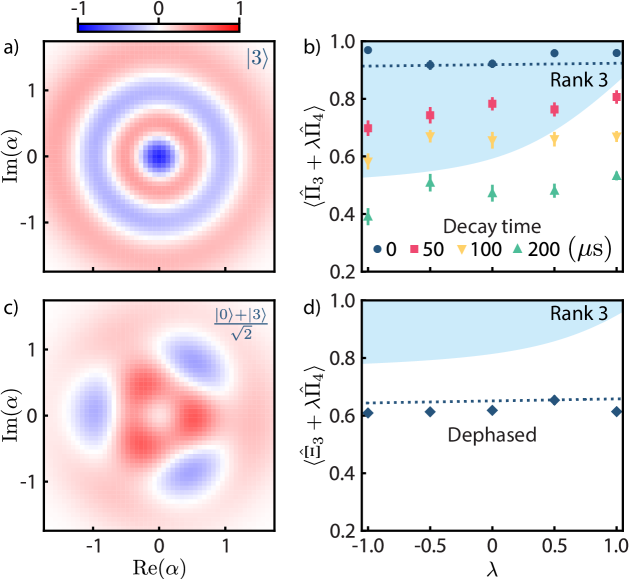
Figure 3: Non-Gaussianity ranking. (a) Reconstructed Wigner plot of the prepared Fock state $|3\rangle$. (b) We probe the non-Gaussianity rank of the prepared Fock state in the oscillator by measuring the observable $\langle\hat{\Pi}_{3}+\lambda\hat{\Pi}_{4}\rangle$ ($\hat{\Pi}_{n}\equiv|n\rangle\langle n|$). The optimized threshold for rank-3 is shown as the lower boundary of the blue shaded region, above which one infers rank-3 states. When the initial state is allowed to decay for a variable amount of time, we find that the outcome of our measurement reflects a loss in rank after around 200 $\mu$s. (c) Reconstructed Wigner plot for the state $(|0\rangle+|3\rangle)/\sqrt{2}$, prepared with added dephasing noise [15]. (d) Measurement of $\langle\hat{\Xi}_{3}+\lambda\hat{\Pi}_{4}\rangle$ ($\hat{\Xi}_{n}\equiv|n\rangle\langle 0|+|0\rangle\langle n|$) is used to quantify the rank. Due to the dephasing, the strength of the off-diagonal elements $\langle\hat{\Xi}_{3}\rangle$ is reduced and the rank becomes undefined. Both in panels (b) and (d), our method OREO shown by the blue markers agrees with values extracted from the full density matrix reconstruction (dotted lines).

Next, we use OREO to efficiently evaluate Fock states and their coherent superpositions, which are critical non-Gaussian resources in CV quantum information processing [3, 20] and entanglement distillation [21, 22]. To benchmark the quality of these resource states in real hardware, it is desirable to have an accurate and experimentally accessible measure of their non-Gaussianity [23, 24, 25]. Here, we adopt the theoretically optimized metric introduced in Ref. [25] where a state is said to have rank n non-Gaussianity if

$$\exists\lambda\mathrel{\mathop{\ordinarycolon}}\langle\hat{\Pi}_{n}+\lambda\hat{\Pi}_{n+1}\rangle>F_{n}(\lambda),$$ (2)

where $F_{n}(\lambda)$ is a calculated threshold [15] and $\hat{\Pi}_{n}$ is the projector onto the n-th Fock state. We use OREO to directly probe this observable for arbitrary $\lambda$ and obtain the corresponding expectation value in Eq. (2).

We demonstrate this experimentally for two specific non-Gaussian resource states. In the first case, a Fock state $|3\rangle$ was prepared using a standard numerically optimized state transfer process [17]. We also performed a standard Wigner tomography and obtained the reconstructed density matrix via Bayesian inference [12], from which we confirm that a state $|3\rangle$ was prepared with high fidelity of $F=0.92(2)$ (Fig. 3a). We then perform OREO and directly extract the value of $\langle\hat{\Pi}_{3}+\lambda\hat{\Pi}_{4}\rangle$ from single-shot qubit measurements for $\lambda=-1,\,-0.5,\,0,\,0.5,\,1$. The measurement outcomes, shown as blue circles in Fig. 3b are considerably above the theoretically calculated threshold $F_{3}(\lambda)$ (lower boundary of the blue shaded region), indicating that the state has non-Gaussianity rank of 3. These results, obtained via a single measurement for each value of $\lambda$, are consistent with the values extracted from the reconstruction of the full density matrix after Wigner tomography (dotted line), which is significantly more costly in measurement time.

To further illustrate the reliability of OREO in identifying the non-Gausianity rank, we execute the same experiment with a variable wait time between state preparation and rank estimation, allowing the oscillator state to decay under single photon loss. For a 200-$\mu$s wait time, which is approximately 18% of single-photon lifetime $T_{1}$ of the cavity [15], we expect significant reduction in the rank of the initial Fock state. Our measurement outcomes, shown as green triangles, show that $\langle\hat{\Pi}_{n}+\lambda\hat{\Pi}_{n+1}\rangle$ is indeed consistently under the threshold and gives a clear confirmation that we can no longer infer that the oscillator state has rank 3. For shorter decay times (red and yellow data points corresponding to 50-$\mu$s and 100-$\mu$s wait time respectively), there are still values of $\lambda$ that satisfy the condition in Eq. (2), allowing the conclusion that the state still has rank 3. Thus, the flexibility afforded by OREO to extract information on the more complex quantity $\langle\hat{\Pi}_{3}+\lambda\hat{\Pi}_{4}\rangle$ provides an accurate and efficient mechanism to determine the non-Gaussianity rank.

This ability to reliably extract the non-Gaussianity rank can also reveal subtle imperfections in the resource state that are otherwise not obvious. For instance, we investigate a target state of $(|0\rangle+|3\rangle)/\sqrt{2}$ in the oscillator and use the observable $\langle\Xi_{3}+\lambda\Pi_{4}\rangle$ with $\Xi_{3}\equiv|3\rangle\langle 0|+|0\rangle\langle 3|$, which captures the coherence of the quantum superposition, to infer its rank. Experimentally, we prepare the target state in the oscillator using a numerically optimized state-transfer pulse [17] and then induce a dephasing mechanism on the cavity via a strong readout pulse which perturbs the oscillator frequency due to a transmon-mediated cross-Kerr interaction [15]. The reconstructed Wigner of the resulting dephased state is shown in Fig. 3c with fidelity $0.79(2)$ to the ideal target state. We then perform OREO and directly probe the value of $\langle\Xi_{3}+\lambda\Pi_{4}\rangle$. The outcome, shown in Fig. 3d, is consistently below the threshold and in close agreement with the full reconstructed density matrix (dotted line), providing a clear indication of the loss of quantum coherence and the corresponding non-Gaussianity rank due to this induced dephasing effect. In contrast, the Wigner function of the reconstructed density matrix (Fig. 3c) still shows three well-defined negative regions that may lead to a naive conclusion that the state has rank 3. Therefore, this example highlights the ability of OREO as a reliable and sensitive diagnosis tool to assess the coherence of non-Gaussian resource states.

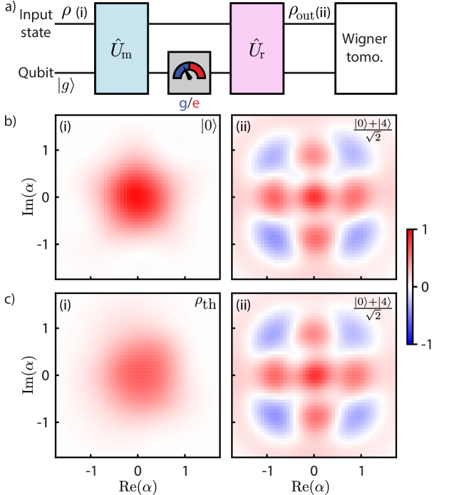
Figure 4: Projection to a target oscillator state. a) The pulse sequence to achieve state projection $\hat{P}_{\psi}=|\psi\rangle\langle\psi|$ after OREO. It involves a second numerically optimized pulse $\hat{U}_{\text{r}}$ that reverts the mapping done by $\hat{U}_{\text{m}}$. The resulting oscillator states after successful projections are characterized using sparse Wigner tomography. (b)-(c) The reconstructed Wigner functions of the initial and final states of the cavity after the projection into the state $|\psi\rangle=(|0\rangle+|4\rangle)/\sqrt{2}$ with the cavity prepared in $|0\rangle$ (b) and in a thermal state with $n_{\text{th}}=0.24$ (c). The projected oscillator states in (b) and (c) have similar fidelities of $0.84(3)$ and $0.85(3)$, respectively, to the ideal binomial state despite the differences in initial conditions.

Finally, we show that OREO can be readily extended to perform a projective measurement and collapse the oscillator state $\rho$ into any target $|\psi\rangle$, which offers an effective state preparation method that is independent of the oscillator’s initial condition. In practice, this feature is realized using a procedure described in Fig. 4a. It builds on the original OREO procedure with an additional operation $\hat{U}_{\text{r}}$ that reverts the mapping of $\hat{U}_{\text{m}}$. Here, the intermediate qubit measurement extracts the overlap observable $p=\langle\psi|\rho|\psi\rangle$ and heralds the correct final state in the oscillator [15].

As an illustration, we optimize $\hat{U}_{\text{m}}$ and $\hat{U}_{\text{r}}$ for the observable $\hat{P}_{\psi}=|\psi\rangle\langle\psi|$, where $|\psi\rangle$ is the binomial state $(|0\rangle+|4\rangle)/\sqrt{2}$. Measurement of the qubit ground state signals a successful projection to the target state, whereas the oscillator state associated with the qubit in $|e\rangle$ is discarded. We execute this procedure with the oscillator initialized in the vacuum state (Fig. 4b(i)) and sparse Wigner tomography performed in the end to obtain the reconstructed density matrix of the output state $\rho_{\text{out}}$. The Wigner plot of the reconstructed density matrix (Fig. 4b(ii)) shows close agreement with the ideal binomial state, with a success rate of $p=0.49$ and fidelity of $0.84(3)$, limited by qubit Ramsey time and measurement imperfections [15].

Next, we prepare the oscillator in a thermal state (Fig. 4c(i)) with mean photon number $n_{\text{th}}=0.24$ with fidelity $0.97(2)$ [15], and perform the same projective operation. The reconstructed Wigner plot of the output state (Fig. 4c(ii)) shows a fidelity of $0.85(3)$ to the ideal binomial state, a clear indication that the quality of the projection is not affected by the initial condition of the oscillator. However, this comes at the cost of a minor reduction in the success rate ($p=0.44$). This simple demonstration shows that the extension of OREO to implement a projection to a target state serves as an effective oscillator state initialization tool. Although it is a heralded process with non-unity success probability, its robustness against the initial condition of the oscillator is a valuable feature that is beyond the reach of the standard state-transfer protocols. This is particularly useful for hardware platforms where the oscillator may not have a well-defined initial state due to the presence of residual thermal excitations such as bosonic cQED [2, 3], opto-mechanical [26], and quantum acoustic [27] devices.

In conclusion, this work demonstrates the robust capabilities of the Optimized Routine for Estimation of any Observable (OREO) in bridging critical measurement gaps in bosonic cQED systems. By harnessing numerically optimized pulses to encode the expectation value of target observables into an auxiliary transmon qubit, OREO enables single-shot detection of a diverse range of oscillator properties, from phase-space quadratures and their higher-order moments to non-Gaussianity metrics. The performance of OREO is mainly limited by qubit decoherence during the optimized drives, which can potentially be alleviated by known methods to extend the qubit coherence properties [28, 29] or reduce the drive durations [30]. Even with our modest system parameters [15], experimental results presented in this work effectively validate OREO’s value and practical viability. Collectively, these findings underscore OREO as a versatile and transformative tool for advancing continuous-variable quantum information processing.

SUPPLEMENTAL MATERIAL

I Device & System Parameters

The device used in this work (Fig. 1 in the main text) is a standard bosonic cQED system operating in the strong-dispersive coupling regime. It consists of a superconducting 3D microwave cavity, an ancillary transmon and a planar readout resonator. The cavity was machined from a block of high-purity (4N) aluminum, while the transmon and readout resonator were fabricated by evaporating aluminum on a sapphire substrate.

The Hamiltonian of the system can be written as

$$\hat{H}=\hat{H}_{0}+\hat{H}_{d},$$ (3)

with the bare and drive terms respectively expressed as

$$\hat{H}_{0}/\hbar = \sum_{k=q,c,r}\omega_{k}\hat{k}^{\dagger}\hat{k}-\frac{\chi_{kk}}{2}\hat{k}^{\dagger}\hat{k}^{\dagger}\hat{k}\hat{k}$$ (4)

$$-\chi_{qc}\hat{q}^{\dagger}\hat{q}\hat{c}^{\dagger}\hat{c}-\chi_{qr}\hat{q}^{\dagger}\hat{q}\hat{r}^{\dagger}\hat{r}-\chi_{cr}\hat{c}^{\dagger}\hat{c}\hat{r}^{\dagger}\hat{r}$$

$$-\chi_{qc}^{\prime}\hat{q}^{\dagger}\hat{q}\hat{c}^{\dagger}\hat{c}^{\dagger}\hat{c}\hat{c},$$

and

$$\hat{H}_{d}/\hbar = \epsilon_{q}(t)\hat{q}e^{i\omega_{dq}t}+\epsilon_{q}^{*}(t)\hat{q}^{\dagger}e^{-i\omega_{dq}t}$$ (5)

$$+\epsilon_{c}(t)\hat{c}e^{i\omega_{dc}t}+\epsilon_{c}^{*}(t)\hat{c}^{\dagger}e^{-i\omega_{dc}t},$$

where we have used $k$ to indicate the qubit ($q$), oscillator ($c$), and resonator ($r$). The operator $\hat{k}$ ($\hat{k}^{\dagger}$) denotes the annihilation (creation) operator of the corresponding system with frequency $\omega_{k}$ and self-Kerr $\chi_{kk}$, $\chi_{qc}$ the qubit-oscillator cross-Kerr or dispersive coupling, $\chi_{qr}$ the qubit-resonator cross-Kerr, $\chi_{cr}$ the oscillator-resonator cross-Kerr, $\chi_{qc}^{\prime}$ the second-order qubit-oscillator dispersive coupling, and $\epsilon_{q}(t)$ ($\epsilon_{c}(t)$) the time-dependent complex drive amplitude of the qubit (oscillator) with frequency $\omega_{dq}$ ($\omega_{dc}$). The experimental values of the Hamiltonian parameters in our system are summarized in Table  1. Note that as the self-Kerr (anharmonicity) of the transmon is high, only the first two energy levels are occupied and it can effectively be treated as a qubit with $|g\rangle$ ($|e\rangle$) as its ground (excited) state.

Description	Label	Value
Cavity frequency	$\omega_{c}/2\pi$	4.641 GHz
Transmon frequency	$\omega_{q}/2\pi$	5.327 GHz
Reasonator frequency	$\omega_{r}/2\pi$	7.568 GHz
Cavity self-Kerr	$\chi_{cc}/2\pi$	4.4 kHz
Transmon self-Kerr	$\chi_{qq}/2\pi$	175.31 MHz
Transmon-cavity cross-Kerr	$\chi_{qc}/2\pi$	1.482 MHz
2nd order correction to $\chi_{qc}$	$\chi^{\prime}_{qc}/2\pi$	13.6 kHz
Transmon-resonator cross-Kerr	$\chi_{qr}/2\pi$	0.49 MHz
Cavity $T_{1}$	$T_{1,c}$	1.1 ms
Transmon $T_{1}$	$T_{1,q}$	100 $\mu$s
Transmon $T_{2}$ Ramsey	$T_{2,q}$	40$\,\mu$s

Table 1: Hamiltonian parameters and coherence times of the bosonic cQED device.

II Proof of Universality

Here we show that any observable $\hat{\mathcal{O}}$ of a harmonic oscillator in any state $\rho$ can be estimated by applying a unitary operation $\hat{U}_{\text{m}}$, from the qubit-oscillator Hamiltonian in Eq. (3) with optimized drives in time, and a qubit measurement.

We start by noting that any observable can be written as $\hat{\mathcal{O}}=\sum_{k}\Lambda_{k}|\psi_{k}\rangle\langle\psi_{k}|$, where $\Lambda_{k}\in\mathbb{R}$ is any real number, and $\{|\psi_{k}\rangle\}$ is any basis. Since the qubit measurement restricts the outcomes to be $\langle\hat{\sigma}_{z}\rangle\in[-1,1]$, we will measure the scaled version

$$\hat{O}=\hat{\mathcal{O}}/f=\sum_{k}\lambda_{k}|\psi_{k}\rangle\langle\psi_{k}|,$$ (6)

where $f=\max_{k}|\Lambda_{k}|$ such that $\lambda_{k}\in[-1,1]$. After the measurements, we obtain the expectation value of the unscaled observable as $\mbox{tr}(\hat{\mathcal{O}}\rho)\equiv\langle\hat{\mathcal{O}}\rangle=f\times\langle\hat{O}\rangle$.

Let the initial qubit-oscillator state be $|g\rangle\langle g|\otimes\rho$, and define the unitary $\hat{U}_{\text{m}}=\hat{U}_{\text{P}}\hat{U}$, where $\hat{U}_{\text{P}}$ implements the Ramsey sequence, which, together with the qubit measurement, realizes the standard parity measurement of the oscillator state [10]. The parity can then be written as

$$P = \text{tr}(\mathbb{I}_{2}\otimes\hat{P}\>\hat{U}\>|g\rangle\langle g|\otimes\rho\>\hat{U}^{\dagger})$$ (7)

$$= \text{tr}(\mathbb{I}_{2}\otimes\hat{P}\>|g\rangle\langle g|\otimes\hat{U}_{\text{c}}\>\rho\>\hat{U}_{\text{c}}^{\dagger})$$

$$= \text{tr}_{\text{c}}(\hat{U}_{\text{c}}^{\dagger}\hat{P}\hat{U}_{\text{c}}\>\rho)$$

$$\equiv \text{tr}_{\text{c}}(\hat{O}_{\text{eff}}\>\rho),$$

where $\hat{P}\equiv\exp(i\hat{c}^{\dagger}\hat{c}\pi)$ denotes the parity operator and $\text{tr}_{\text{c}}$ the trace with respect to the oscillator, and the steps are explained as follows: for the second line, we use the fact that the Hamiltonian in Eq. (3) with optimized drives can realize any unitary $\hat{U}_{\text{c}}$ on the oscillator [16], i.e., $\hat{U}\>|g\rangle\langle g|\otimes\rho\>\hat{U}^{\dagger}=|g\rangle\langle g|\otimes\hat{U}_{\text{c}}\>\rho\>\hat{U}_{\text{c}}^{\dagger}$; the cyclic property of trace and partial trace with respect to the qubit are used in the third line; and effective observable is defined in the fourth line as $\hat{O}_{\text{eff}}=\hat{U}_{\text{c}}^{\dagger}\hat{P}\hat{U}_{\text{c}}$.

In realistic situations, one can choose a sufficient truncation dimension $D$ within which the arbitrary state of the oscillator can be fully expressed. Consequently, the observable of interest is also truncated within $D$, which can be arbitrarily chosen. Now we show that any observable within dimension $D$,

$$\hat{O}=\sum_{k=0}^{D-1}\lambda_{k}|\psi_{k}\rangle\langle\psi_{k}|$$ (8)

with $\{|\psi_{k}\rangle\}$ being a basis within $D$, can be achieved by applying the universal unitary on the parity operator, as defined in Eq. (7). First, we note that the parity operator can be expressed as $\hat{P}=\sum_{n=0}^{\infty}(-1)^{n}|n\rangle\langle n|$ with $\{|n\rangle\}$ being the Fock basis. As any unitary on the oscillator is possible, there exists $\hat{U}_{\text{c}}^{\dagger}$ that applies the following transformation

$$|0\rangle \rightarrow \alpha_{0}|\psi_{0}\rangle+\beta_{0}|h_{1}\rangle$$

$$|h_{1}\rangle \rightarrow \beta_{0}|\psi_{0}\rangle-\alpha_{0}|h_{1}\rangle$$

$$|1\rangle \rightarrow \alpha_{1}|\psi_{1}\rangle+\beta_{1}|h_{2}\rangle$$

$$|h_{2}\rangle \rightarrow \beta_{1}|\psi_{1}\rangle-\alpha_{1}|h_{2}\rangle$$ (9)

$$\vdots$$

for any $\alpha_{n},\beta_{n}\in\mathbb{R}$ with $\alpha_{n}^{2}+\beta_{n}^{2}=1$, where we have used $|h_{n}\rangle$ to denote Fock state outside of the truncation dimension $D$, starting from $|h_{1}\rangle$ with parity $-1$. It can be seen that the LHS and RHS in Eqs. (9) each consists of states that form a complete basis. Within the dimension $D$, we then have

$$\hat{O}_{\text{eff}}=\sum_{k=0}^{D-1}(-1)^{k}(\alpha_{k}^{2}-\beta_{k}^{2})|\psi_{k}\rangle\langle\psi_{k}|,$$ (10)

where $(-1)^{k}(\alpha_{k}^{2}-\beta_{k}^{2})\in[-1,1]$. These coefficients can be arbitrary for all $k$s as any unitary $\hat{U}_{\text{c}}^{\dagger}$ is possible, which completes the proof.

Additionally, the relation between parity and qubit measurement, following the Ramsey sequence [10], is given by $P=-\langle\hat{\sigma}_{z}\rangle=1-2p_{g}$, where $p_{g}$ is the probability of the qubit being in the ground state. If one post processes $p_{g}$ instead of $\langle\hat{\sigma}_{z}\rangle$, we have $p_{g}=(1-P)/2=\text{tr}_{\text{c}}(\sum_{k}(1-\lambda_{k})/2\>|\psi_{k}\rangle\langle\psi_{k}|\>\rho)$, where $(1-\lambda_{k})/2\in[0,1]$ and the corresponding observable $\sum_{k}(1-\lambda_{k})/2\>|\psi_{k}\rangle\langle\psi_{k}|$ is positive.

III Implementation of OREO

Here, we provide the detailed recipe of the OREO protocol for the estimation of any observable, as depicted in Fig. 1, as well as the state projection protocol, as depicted in Fig. 4a.

III.1 Observable estimation

For estimation of an arbitrary observable we apply an optimized unitary $\hat{U}_{\text{m}}$ to the initial state $|g\rangle\langle g|\otimes\rho$ followed by a qubit measurement. The latter can then be written as

$$\langle\hat{\sigma}_{z}\rangle = 2p_{g}-1$$ (11)

$$= 2\text{tr}(|g\rangle\langle g|\otimes\mathbb{I}_{\text{c}}\>\hat{U}_{\text{m}}\>|g\rangle\langle g|\otimes\rho\>\hat{U}_{\text{m}}^{\dagger})-1$$

$$= \text{tr}_{\text{c}}\left((2\langle g|\hat{U}_{\text{m}}^{\dagger}|g\rangle\langle g|\hat{U}_{\text{m}}|g\rangle-\mathbb{I}_{\text{c}})\rho\right),$$

where we have used the partial trace with respect to the qubit and the cyclic property of trace. Given an arbitrary observable $\hat{\mathcal{O}}$ with $\hat{O}$ as its scaled version truncated to dimension $D$ (see Eq. (8)), we optimize the unitary $\hat{U}_{\text{m}}$ such that $\hat{O}_{\text{eff}}=\hat{O}$, where

$$\hat{O}_{\text{eff}}\equiv 2\langle g|\hat{U}_{\text{m}}^{\dagger}|g\rangle\langle g|\hat{U}_{\text{m}}|g\rangle-\mathbb{I}_{\text{c}}$$ (12)

truncated to dimension $D$.

As explained in the previous section, if the observable is positive, one can post process $p_{g}$ instead of $\langle\hat{\sigma}_{z}\rangle$. In this case, we have $p_{g}=\text{tr}_{\text{c}}(\langle g|\hat{U}_{\text{m}}^{\dagger}|g\rangle\langle g|\hat{U}_{\text{m}}|g\rangle\>\rho)$, and the effective observable now reads

$$\hat{O}_{\text{eff}}\equiv\langle g|\hat{U}_{\text{m}}^{\dagger}|g\rangle\langle g|\hat{U}_{\text{m}}|g\rangle$$ (13)

truncated to dimension $D$.

The optimization is performed similar to the GRAPE method [17], i.e., optimizing the amplitude of the drives $\{\epsilon_{q}(t),\epsilon_{c}(t)\}$ in time with gradient descent to minimize a cost function. In the present case, the cost function is

$$\mathcal{C}=\sum_{ij}|(\hat{O}-\hat{O}_{\text{eff}})_{ij}|^{2},$$ (14)

where $ij$ denotes the $(i,j)$-th matrix element. This cost function ensures that all elements of $\hat{O}_{\text{eff}}$ be close to those of the target observable $\hat{O}$ within the chosen truncation dimension $D$.

III.2 State projection

Here, we will focus on the case where $\hat{O}=|\psi\rangle\langle\psi|$. This corresponds to a projective measurement, where the goal is twofold: to extract the probability of overlap $\langle\psi|\rho|\psi\rangle$ and have the oscillator state collapse to $|\psi\rangle$. The sequence for this is presented in Fig. 4a, where a second unitary $\hat{U}_{r}$ is introduced to obtain the collapsed cavity state.

As the observable is positive, to get the probability of overlap, we use Eq. (13), where the qubit measurement reads

$$p_{g} = \text{tr}_{\text{c}}(\langle g|\hat{U}_{\text{m}}^{\dagger}|g\rangle\langle g|\hat{U}_{\text{m}}|g\rangle\>\rho)$$ (15)

$$= \text{tr}_{\text{c}}(|\psi\rangle\langle\psi|\>\rho)$$

$$= \langle\psi|\rho|\psi\rangle.$$

In a single-shot manner, state of the oscillator after the qubit measurement $\tilde{\rho}_{\text{c}|j}$ depends on the outcome, whether the qubit is in the ground state $j=g$ or excited state $j=e$. In the case of the former, the qubit-oscillator state after the qubit measurement can be written as

$$\tilde{\rho}_{\text{qc}|g} = \frac{|g\rangle\langle g|\otimes\mathbb{I}_{\text{c}}\>\hat{U}_{\text{m}}\>|g\rangle\langle g|\otimes\rho\>\hat{U}_{\text{m}}^{\dagger}\>|g\rangle\langle g|\otimes\mathbb{I}_{\text{c}}}{p_{g}}$$ (16)

$$= |g\rangle\langle g|\otimes\frac{\langle g|\hat{U}_{\text{m}}|g\rangle\rho\langle g|\hat{U}_{\text{m}}^{\dagger}|g\rangle}{p_{g}}$$

$$= |g\rangle\langle g|\otimes\tilde{\rho}_{\text{c}|g}.$$

We note that although the oscillator state at this point is pure, as one can confirm that $\text{tr}(\tilde{\rho}_{\text{c}|g}^{2})=1$, it is not yet in the target projected state $|\psi\rangle$. This is where the second unitary $\hat{U}_{\text{r}}$ comes into play, after which the qubit-oscillator state can be written as

$$\rho_{\text{qc}|g} = \frac{\hat{U}_{\text{r}}\>|g\rangle\langle g|\otimes\mathbb{I}_{\text{c}}\>\hat{U}_{\text{m}}\>|g\rangle\langle g|\otimes\rho\>\hat{U}_{\text{m}}^{\dagger}\>|g\rangle\langle g|\otimes\mathbb{I}_{\text{c}}\>\hat{U}_{\text{r}}^{\dagger}}{p_{g}}.$$ (17)

The probability of the qubit being in ground state here is

$$p_{g|g} = \text{tr}(|g\rangle\langle g|\otimes\mathbb{I}_{\text{c}}\>\rho_{\text{qc}|g})$$ (18)

$$= \text{tr}_{\text{c}}\left(\frac{\langle g|\hat{U}_{\text{r}}|g\rangle\langle g|\hat{U}_{\text{m}}|g\rangle\rho\langle g|\hat{U}_{\text{m}}^{\dagger}|g\rangle\langle g|\hat{U}_{\text{r}}^{\dagger}|g\rangle}{p_{g}}\right),$$

where we carried out the partial trace with respect to the qubit. If the second unitary can be optimized such that $\hat{U}_{\text{r}}=\hat{U}_{\text{m}}^{\dagger}$, then the probability reduces to

$$p_{g|g} = \text{tr}_{\text{c}}\left(\frac{|\psi\rangle\langle\psi|\rho|\psi\rangle\langle\psi|}{p_{g}}\right)$$ (19)

$$= 1,$$

which means the qubit is in its ground state decoupled from the oscillator, i.e., $\rho_{\text{qc}|g}=|g\rangle\langle g|\otimes\rho_{\text{out}|g}$. It is easy to see that

$$\rho_{\text{out}|g} = \langle g|\rho_{\text{qc}|g}|g\rangle$$ (20)

$$= |\psi\rangle\langle\psi|.$$

To arrive at this collapsed state, it is not necessary to have $\hat{U}_{\text{r}}=\hat{U}_{\text{m}}^{\dagger}$. In fact, it is sufficient to optimize the reverse unitary in the oscillator space only such that $\langle g|\hat{U}_{\text{r}}|g\rangle=\langle g|\hat{U}_{\text{m}}^{\dagger}|g\rangle$, which is what we implemented in our experiments. In particular, given the unitary $\hat{U}_{\text{m}}$ that is optimized previously, we optimize the reverse unitary in the same way as described in Eq. (14) by minimizing the cost function

$$\mathcal{C}=\sum_{ij}|(\hat{M}_{1}-\hat{M}_{2})_{ij}|^{2},,$$ (21)

where $\hat{M}_{1}$ $(\hat{M}_{2})$ denotes $\langle g|\hat{U}_{\text{m}}^{\dagger}|g\rangle$ ($\langle g|\hat{U}_{\text{r}}|g\rangle$) truncated to dimension $D$.

In the case where the qubit measurement yields excited state, the qubit-oscillator state after the operation $\hat{U}_{\text{r}}$ reads

$$\rho_{\text{qc}|e} = \frac{\hat{U}_{\text{r}}\>|e\rangle\langle e|\otimes\mathbb{I}_{\text{c}}\>\hat{U}_{\text{m}}\>|g\rangle\langle g|\otimes\rho\>\hat{U}_{\text{m}}^{\dagger}\>|e\rangle\langle e|\otimes\mathbb{I}_{\text{c}}\>\hat{U}_{\text{r}}^{\dagger}}{1-p_{g}}.$$ (22)

The probability of the qubit being in the ground state here is

$$p_{g|e} = \text{tr}(|g\rangle\langle g|\otimes\mathbb{I}_{\text{c}}\>\rho_{\text{qc}|e})$$ (23)

$$= \text{tr}_{\text{c}}\left(\frac{\langle g|\hat{U}_{\text{r}}|e\rangle\langle e|\hat{U}_{\text{m}}|g\rangle\rho\langle g|\hat{U}_{\text{m}}^{\dagger}|e\rangle\langle e|\hat{U}_{\text{r}}^{\dagger}|g\rangle}{1-p_{g}}\right),$$

where the partial trace with respect to the qubit has been carried out. If $\hat{U}_{\text{r}}=\hat{U}_{\text{m}}^{\dagger}$, the probability reduces to

$$p_{g|e} = \text{tr}_{\text{c}}\left(\frac{(\mathbb{I}_{\text{c}}-|\psi\rangle\langle\psi|)\rho(\mathbb{I}_{\text{c}}-|\psi\rangle\langle\psi|)}{1-p_{g}}\right)$$ (24)

$$= 1,$$

where we have used $\langle g|\hat{U}_{\text{m}}^{\dagger}|e\rangle\langle e|\hat{U}_{\text{m}}|g\rangle=\langle g|\hat{U}_{\text{m}}^{\dagger}(\mathbb{I}_{2}-|g\rangle\langle g|)\hat{U}_{\text{m}}|g\rangle=\mathbb{I}_{c}-|\psi\rangle\langle\psi|$. Consequently, the qubit-oscillator state is of the form $\rho_{\text{qc}|e}=|g\rangle\langle g|\otimes\rho_{\text{out}|e}$, where

$$\rho_{\text{out}|e} = \langle g|\rho_{\text{qc}|e}|g\rangle$$ (25)

$$= \frac{(\mathbb{I}_{\text{c}}-|\psi\rangle\langle\psi|)\rho(\mathbb{I}_{\text{c}}-|\psi\rangle\langle\psi|)}{1-p_{g}}$$

$$= \frac{1}{1-\langle\psi|\rho|\psi\rangle}\sum_{|i\rangle,|j\rangle\neq|\psi\rangle}\langle i|\rho|j\rangle\>|i\rangle\langle j|.$$

This is the not-$|\psi\rangle$ state, which erases the $|\psi\rangle$ state component from $\rho$ and retains all elements orthogonal to $|\psi\rangle$. For example, if the input states we are dealing with are qubit codes $\{|\psi\rangle,|\phi\rangle\}$, i.e., two orthogonal states encoded in the oscillator (popular for bosonic error correction schemes [4, 5, 6]), the outcome of the qubit in excited state will correspond to the state $|\phi\rangle$. However, equation (25) requires the complete inversion of the first qubit-oscillator unitary, $\hat{U}_{\text{r}}=\hat{U}_{\text{m}}^{\dagger}$, which is not viable in our current setup. One way to do this is by having the option to flip the sign of the Hamiltonian. With flux tunability on the qubit frequency [31], one might be able to flip the sign of the dispersive coupling $\chi_{\text{qc}}$ [32], which is the dominant term in the bare Hamiltonian $\hat{H}_{0}$, and therefore, allowing the required unitary inversion.

IV Simulation of imperfections

In this section, we explore the effect of various forms of imperfections on OREO. The system was modeled using a standard master equation simulation using the parameters listed in Table 1 unless otherwise stated.

IV.1 Hamiltonian parameter miscalibration

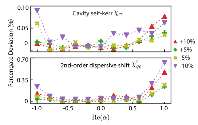
Figure 5: Effect of potential differences between the estimated and actual values of $\chi_{cc}$ and $\chi^{\prime}_{qc}$ on $\langle x\rangle$ observable measurement

Extracting the higher-order Hamiltonian terms ($\chi_{cc}$ and $\chi^{\prime}_{qc}$) of the system to a high degree of precision is experimentally challenging. As a result, the actual values might deviate from the estimated values by a non-negligible amount. To study the robustness of the protocol to such errors, we simulated the $\langle x\rangle$ measurement using values of $\chi_{cc}$ and $\chi^{\prime}_{qc}$ that were $\pm 5{-}10\%$ from the estimated values used to generate the GRAPE pulse. From Fig. 5, we can see that the effects of these miscalibrations are small ($<1\%$).

IV.2 Losses during GRAPE pulses

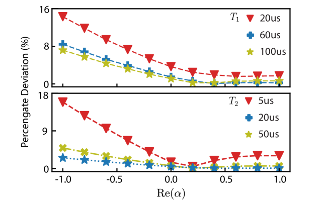
Figure 6: Effect of qubit $T_{1}$ and $T_{2}$ on $\langle x\rangle$ the values of the phase-space quadrature obtained via OREO.

We investigate the impact of transmon decoherence on the performance of OREO. As a reference, we compare simulations of the $\langle x\rangle$ measurement with different $T_{1}$ and $T_{2}$ to simulations with a lossless transmon. In Fig. 6, we observe significant deviations from the lossless case with typical coherence times in our devices, that is, $T_{1}\approx 100\,\mu$s and $T_{2}\approx 40\text{-}50\,\mu$s. Thus, the performance of OREO will directly benefit from the mainstream pursuits of the cQED community to continually improve the qubit coherence properties. Furthermore, we also observe that the errors become more pronounced when the coherence state is displaced further out in the phase space. This is consistent with our analysis that the choice of truncation dimension is a crucial factor in OREO to ensure its reliability.

V Calibration and correction for readout assignment error

As the value of the observable is directly mapped to the qubit state, it is important to account for qubit state assignment (readout) errors. To characterize the readout error, we first prepare the qubit in the $|g\rangle$ ($|e\rangle$) state and measure the $|e\rangle$ population to obtain $p_{ge}$ ($p_{ee}$), which was found to be 0.02 (0.96). This value is then used to offset (scale) the measured excited population using the formula:

$$p_{e}^{\text{corrected}}=\frac{p_{e}^{\text{measured}}-p_{ge}}{p_{ee}}$$ (26)

VI non-Gaussianity threshold

Non-Gaussian states are those whose Wigner functions deviate from a Gaussian shape and can exhibit features such as negative values in their Wigner function. These states are resources for universal quantum computing [1], quantum error correction [4, 5, 6], and quantum metrology [7, 8]. Some non-Gaussian states are more useful than others, and therefore, it is important to probe the non-Gaussianity hierarchy.

In this work, we explore a hierarchy of $n$-photon quantum non-Gaussianity, which asserts that a state with a non-Gaussianity rank of $n$ is incompatible with any mixture of Fock state superpositions up to Fock $|n-1\rangle$ with the addition of any application of Gaussian operation [33, 34]. Mathematically, a pure state $|\psi\rangle$ is said to have rank $n$ if it cannot be written as

$$|\psi\rangle\neq\hat{G}|\tilde{\psi}_{n-1}\rangle,$$ (27)

where $\hat{G}$ is a Gaussian operation, which can be implemented by a displacement and/or squeezing operation, and $|\tilde{\psi}_{n-1}\rangle=\sum_{k=0}^{n-1}c_{k}|k\rangle$ is arbitrary superposition of Fock states up to Fock $|n-1\rangle$.

To probe the rank experimentally, we measure a single observable $\hat{O}$. For an arbitraty state $\rho$, if the expectation value of the observable $\langle\hat{O}\rangle_{\rho}>F_{n}$, where $F_{n}$ is the rank-$n$ threshold, one concludes that the state has rank $n$. The threshold $F_{n}$ is computed numerically by optimizing the observable $\langle\hat{O}\rangle$ given the state $\hat{G}|\tilde{\psi}_{n-1}\rangle$ over the parameters of the Gaussian operation and superposition weights $\{c_{k}\}$ as in Ref. [25]. We chose an observable $\hat{O}=\hat{\Pi}_{3}+\lambda\hat{\Pi}_{4}$, where $\hat{\Pi}_{n}\equiv|n\rangle\langle n|$ and $\lambda$ is a free real parameter, to probe rank 3 non-Gaussianity of Fock state $|3\rangle$ (the target in our experiment). This choice is motivated by the incorporation of successful probability $\langle\hat{\Pi}_{3}\rangle$ and a leakage error $\langle\hat{\Pi}_{4}\rangle$ into a higher Fock state. Similarly, for the superposition of Fock state $(|0\rangle+|3\rangle)/\sqrt{2}$, we chose the observable $\hat{O}=\hat{\Xi}_{3}+\lambda\hat{\Pi}_{4}$, where $\hat{\Xi}_{n}\equiv|0\rangle\langle n|+|n\rangle\langle 0|$, capturing the amplitude of the off-diagonal elements. The numerically optimized thresholds for $\hat{\Pi}_{3}+\lambda\hat{\Pi}_{4}$ and $\hat{\Xi}_{3}+\lambda\hat{\Pi}_{4}$ are shown as the lower boundary of the blue shaded region in Figs. 3b and 3d in the main text.

VII Impact of induced dephasing on superpositions of Fock States

The cross-Kerr interaction term $-\chi_{cr}\hat{c}^{\dagger}\hat{c}\hat{r}^{\dagger}\hat{r}$ between the cavity and the readout resonator causes the state in the cavity to dephase when a pulse is applied to the readout resonator. This is a device-specific imperfection which we have exploited to introduce the engineered dephasing on the cavity state. The amount of the dephasing introduced depends on the amplitude and duration of the readout. In this investigation, we experimented with two measurement pulses of the same duration but different amplitude. As shown in Fig. 7, the resulting dephasing reflected by the reduction in the off-diagonal elements is more pronounced when we use a pulse with higher amplitude, i.e. more photons in the readout resonator.

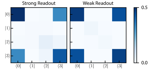
Figure 7: Real components of the reconstructed density matrix of the $|0\rangle+|3\rangle$ state under strong (weak) readout. The strong readout pulse results in a larger dephasing effect which can be observed by the higher reduction of the off-diagonal $|0\rangle\langle 3|$ and $|3\rangle\langle 0|$ components. The amplitude of the weak readout pulse was $\approx 42\%$ of the strong readout pulse.

VIII Preparation of thermal state

The thermal state was prepared by first initializing the transmon in $|g\rangle$ and the cavity in $|\alpha=0.5\rangle$. To induce decoherence in the cavity state, a $\pi/2$-pulse is applied to the transmon to put it into a superposition $(|g\rangle+|e\rangle)/\sqrt{2}$. The system is then allowed to evolve for $\tau=452$ns. The dispersive interaction between the cavity and the transmon causes the system to form an entangled state which decoheres into a statistical mixture due to transmon decoherence [31]. To further amplify this effect, the readout resonator is populated, causing faster transmon decoherence [35]. This process is repeated 40 times. Finally, the transmon is projected to the $|g\rangle$ state which leaves the cavity in a state that is close to a thermal state with a mean photon number $n_{\text{th}}=0.24$.

IX Sequential projections

The projective measurement experiment in the main text can be further extended by performing two projective measurements in a row to increase the yield of successful projections to the $|\psi\rangle=(|0\rangle+|4\rangle)/\sqrt{2}$ state. Although a failed projection leads to a state with a very small $|\psi\rangle$ component, a displacement pulse $\hat{D}(\alpha=-1)$ played to the cavity can take it to a non-orthogonal state, increasing the probability of success in the next iteration.

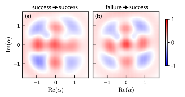
Figure 8: Reconstructed Wigner functions of the final cavity states after two rounds of projective measurements for the cases where (a) the qubit is measured in $|g\rangle$ during both iterations and (b) the qubit is measured in $|e\rangle$ after the first iteration and in $|g\rangle$ after the second one.

Fig. 8 shows the reconstructed Wigner functions of the final state at the end of 2 iterations. The fidelity of the final state after 2 successful projections to the ideal binomial state was about 0.77 while the fidelity of the state with 1 failed and 1 successful projection was about 0.70. This reduction in fidelity is consistent with the limit imposed by transmon decoherence during the repeated applications of the numerically optimized pulses.

References

- Braunstein and Van Loock [2005] S. L. Braunstein and P. Van Loock, Quantum information with continuous variables, Reviews of modern physics 77, 513 (2005).
- Joshi et al. [2021] A. Joshi, K. Noh, and Y. Y. Gao, Quantum information processing with bosonic qubits in circuit qed, Quantum Science and Technology 6, 033001 (2021).
- Copetudo et al. [2024] A. Copetudo, C. Y. Fontaine, F. Valadares, and Y. Y. Gao, Shaping photons: Quantum information processing with bosonic cqed, Applied Physics Letters 124 (2024).
- Ofek et al. [2016] N. Ofek, A. Petrenko, R. Heeres, P. Reinhold, Z. Leghtas, B. Vlastakis, Y. Liu, L. Frunzio, S. M. Girvin, L. Jiang, et al., Extending the lifetime of a quantum bit with error correction in superconducting circuits, Nature 536, 441 (2016).
- Sivak et al. [2023] V. Sivak, A. Eickbusch, B. Royer, S. Singh, I. Tsioutsios, S. Ganjam, A. Miano, B. Brock, A. Ding, L. Frunzio, et al., Real-time quantum error correction beyond break-even, Nature 616, 50 (2023).
- Ni et al. [2023] Z. Ni, S. Li, X. Deng, Y. Cai, L. Zhang, W. Wang, Z.-B. Yang, H. Yu, F. Yan, S. Liu, et al., Beating the break-even point with a discrete-variable-encoded logical qubit, Nature 616, 56 (2023).
- Pan et al. [2025] X. Pan, T. Krisnanda, A. Duina, K. Park, P. Song, C. Y. Fontaine, A. Copetudo, R. Filip, and Y. Y. Gao, Realization of versatile and effective quantum metrology using a single bosonic mode, PRX Quantum 6, 010304 (2025).
- Deng et al. [2024] X. Deng, S. Li, Z.-J. Chen, Z. Ni, Y. Cai, J. Mai, L. Zhang, P. Zheng, H. Yu, C.-L. Zou, et al., Quantum-enhanced metrology with large fock states, Nature Physics 20, pages1874 (2024).
- Schuster et al. [2007] D. Schuster, A. A. Houck, J. Schreier, A. Wallraff, J. Gambetta, A. Blais, L. Frunzio, J. Majer, B. Johnson, M. Devoret, et al., Resolving photon number states in a superconducting circuit, Nature 445, 515 (2007).
- Sun et al. [2014] L. Sun, A. Petrenko, Z. Leghtas, B. Vlastakis, G. Kirchmair, K. Sliwa, A. Narla, M. Hatridge, S. Shankar, J. Blumoff, et al., Tracking photon jumps with repeated quantum non-demolition parity measurements, Nature 511, 444 (2014).
- Campagne-Ibarcq et al. [2020] P. Campagne-Ibarcq, A. Eickbusch, S. Touzard, E. Zalys-Geller, N. E. Frattini, V. V. Sivak, P. Reinhold, S. Puri, S. Shankar, R. J. Schoelkopf, et al., Quantum error correction of a qubit encoded in grid states of an oscillator, Nature 584, 368 (2020).
- Krisnanda et al. [2025] T. Krisnanda, C. Y. Fontaine, A. Copetudo, P. Song, K. X. Lee, N.-N. Huang, F. Valadares, T. C. Liew, and Y. Y. Gao, Demonstrating efficient and robust bosonic state reconstruction via optimized excitation counting, PRX Quantum 6, 010303 (2025).
- Pan et al. [2023] X. Pan, J. Schwinger, N.-N. Huang, P. Song, W. Chua, F. Hanamura, A. Joshi, F. Valadares, R. Filip, and Y. Y. Gao, Protecting the quantum interference of cat states by phase-space compression, Physical Review X 13, 021004 (2023).
- Blais et al. [2004] A. Blais, R.-S. Huang, A. Wallraff, S. M. Girvin, and R. J. Schoelkopf, Cavity quantum electrodynamics for superconducting electrical circuits: An architecture for quantum computation, Physical Review A—Atomic, Molecular, and Optical Physics 69, 062320 (2004).
- [15] See the Supplemental Material for details regarding: device and system parameters; proof of universality; implementation of OREO; simulation of imperfections; calibration and correction for readout assignment error; non-Gaussianity threshold; impact of induced dephasing on superpositions of Fock states; preparation of thermal state; and sequential projections.
- Krastanov et al. [2015] S. Krastanov, V. V. Albert, C. Shen, C.-L. Zou, R. W. Heeres, B. Vlastakis, R. J. Schoelkopf, and L. Jiang, Universal control of an oscillator with dispersive coupling to a qubit, Physical Review A 92, 040303 (2015).
- Heeres et al. [2017] R. W. Heeres, P. Reinhold, N. Ofek, L. Frunzio, L. Jiang, M. H. Devoret, and R. J. Schoelkopf, Implementing a universal gate set on a logical qubit encoded in an oscillator, Nature communications 8, 94 (2017).
- Mihaescu et al. [2020] T. Mihaescu, H. Kampermann, G. Gianfelici, A. Isar, and D. Bruß, Detecting entanglement of unknown continuous variable states with random measurements, New Journal of Physics 22, 123041 (2020).
- Moore et al. [2019] D. W. Moore, A. A. Rakhubovsky, and R. Filip, Estimation of squeezing in a nonlinear quadrature of a mechanical oscillator, New Journal of Physics 21, 113050 (2019).
- Lloyd and Braunstein [1999] S. Lloyd and S. L. Braunstein, Quantum computation over continuous variables, Physical Review Letters 82, 1784 (1999).
- Genoni and Paris [2010] M. G. Genoni and M. G. Paris, Quantifying non-gaussianity for quantum information, Physical Review A—Atomic, Molecular, and Optical Physics 82, 052341 (2010).
- Browne et al. [2003] D. E. Browne, J. Eisert, S. Scheel, and M. B. Plenio, Driving non-gaussian to gaussian states with linear optics, Physical Review A 67, 062320 (2003).
- Fiurášek [2022] J. Fiurášek, Efficient construction of witnesses of the stellar rank of nonclassical states of light, Optics Express 30, 30630 (2022).
- Chabaud et al. [2020] U. Chabaud, D. Markham, and F. Grosshans, Stellar representation of non-gaussian quantum states, Physical Review Letters 124, 063605 (2020).
- Lachman et al. [2019] L. Lachman, I. Straka, J. Hloušek, M. Ježek, and R. Filip, Faithful hierarchy of genuine n-photon quantum non-gaussian light, Physical review letters 123, 043601 (2019).
- Aspelmeyer et al. [2014] M. Aspelmeyer, T. J. Kippenberg, and F. Marquardt, Cavity optomechanics, Reviews of Modern Physics 86, 1391 (2014).
- Wollack et al. [2022] E. A. Wollack, A. Y. Cleland, R. G. Gruenke, Z. Wang, P. Arrangoiz-Arriola, and A. H. Safavi-Naeini, Quantum state preparation and tomography of entangled mechanical resonators, Nature 604, 463 (2022).
- Place et al. [2021] A. P. Place, L. V. Rodgers, P. Mundada, B. M. Smitham, M. Fitzpatrick, Z. Leng, A. Premkumar, J. Bryon, A. Vrajitoarea, S. Sussman, et al., New material platform for superconducting transmon qubits with coherence times exceeding 0.3 milliseconds, Nature communications 12, 1779 (2021).
- Somoroff et al. [2023] A. Somoroff, Q. Ficheux, R. A. Mencia, H. Xiong, R. Kuzmin, and V. E. Manucharyan, Millisecond coherence in a superconducting qubit, Physical Review Letters 130, 267001 (2023).
- Kudra et al. [2022] M. Kudra, M. Kervinen, I. Strandberg, S. Ahmed, M. Scigliuzzo, A. Osman, D. P. Lozano, M. O. Tholén, R. Borgani, D. B. Haviland, et al., Robust preparation of wigner-negative states with optimized snap-displacement sequences, PRX Quantum 3, 030301 (2022).
- Valadares et al. [2024] F. Valadares, N.-N. Huang, K. T. N. Chu, A. Dorogov, W. Chua, L. Kong, P. Song, and Y. Y. Gao, On-demand transposition across light-matter interaction regimes in bosonic cqed, Nature Communications 15, 5816 (2024).
- Blais et al. [2021] A. Blais, A. L. Grimsmo, S. M. Girvin, and A. Wallraff, Circuit quantum electrodynamics, Rev. Mod. Phys. 93, 025005 (2021).
- Bimbard et al. [2010] E. Bimbard, N. Jain, A. MacRae, and A. Lvovsky, Quantum-optical state engineering up to the two-photon level, Nature Photonics 4, 243 (2010).
- Yukawa et al. [2013] M. Yukawa, K. Miyata, T. Mizuta, H. Yonezawa, P. Marek, R. Filip, and A. Furusawa, Generating superposition of up-to three photons for continuous variable quantum information processing, Optics express 21, 5529 (2013).
- Sears et al. [2012] A. P. Sears, A. Petrenko, G. Catelani, L. Sun, H. Paik, G. Kirchmair, L. Frunzio, L. I. Glazman, S. M. Girvin, and R. J. Schoelkopf, Photon shot noise dephasing in the strong-dispersive limit of circuit qed, Phys. Rev. B 86, 180504 (2012).