BeamLLM: Vision-Empowered mmWave Beam Prediction with Large Language Models

Abstract

In this paper, we propose BeamLLM, a vision-aided millimeter-wave (mmWave) beam prediction framework leveraging large language models (LLMs) to address the challenges of high training overhead and latency in mmWave communication systems. By combining computer vision (CV) with LLMs’ cross-modal reasoning capabilities, the framework extracts user equipment (UE) positional features from RGB images and aligns visual-temporal features with LLMs’ semantic space through reprogramming techniques. Evaluated on a realistic vehicle-to-infrastructure (V2I) scenario, the proposed method achieves $61.01\%$ top-$1$ accuracy and $97.39\%$ top-$3$ accuracy in standard prediction tasks, significantly outperforming traditional deep learning models. In few-shot prediction scenarios, the performance degradation is limited to $12.56\%$ (top-$1$) and $5.55\%$ (top-$3$) from time sample $1$ to $10$, demonstrating superior prediction capability.

I Introduction

Millimeter-wave (mmWave) communication has garnered significant attention due to its abundant spectrum resources above $26$ GHz, enabling high-speed data transmission. However, the high operating frequency results in substantial path loss. To address this challenge, massive multiple-input multiple-output (mMIMO) antenna arrays are extensively employed, which utilize highly directional beamforming techniques to mitigate propagation losses. Furthermore, the short wavelength of mmWave signals facilitates compact antenna spacing, which enables the integration of large-scale antenna arrays within constrained physical dimensions. The effectiveness of directional beamforming depends on precise alignment between transmit and receive beams. Beam training addresses this challenge by scanning predefined codebooks at both the transmitter and receiver to identify the optimal beam pair, thereby maximizing received signal power without requiring the exhaustive acquisition of full channel state information (CSI).

Compared to legacy sub-6 GHz MIMO systems, beam training in mmWave systems faces heightened challenges: 1) Large antenna arrays lead to high-dimensional channel matrices, increasing training overhead; 2) Frequent beam tracking, especially in high-mobility scenarios (e.g., vehicle-to-everything (V2X) and unmanned aerial vehicles (UAVs)), introduces prohibitive latency. Recent studies [1, 2, 3, 4] have explored sensing-aided beam prediction, leveraging multimodal sensor data such as RGB images, radar, LiDAR, and GPS to improve efficiency and reduce training overhead. As a key enabler of integrated sensing and communication (ISAC) in 6G, this approach holds significant potential to enhance the performance of mmWave MIMO systems.

To maintain beam prediction performance, deep learning (DL) is commonly used to extract user equipment (UE) movement features from received sensing data, enabling more accurate future beam selection. Due to its powerful non-linear feature extraction capability, DL has been widely explored in wireless communication tasks, including channel estimation[5] and beam prediction. Recent breakthroughs in large language models (LLMs), such as GPT-4[6] and DeepSeek[7], have demonstrated remarkable contextual reasoning and few-shot generalization abilities. While LLMs are originally designed for natural language processing (NLP), LLMs have shown strong cross-modal learning capabilities, thus extending their applications to time series for forecasting and computer vision (CV) tasks.

Inspired by these advantages of the LLMs, several methods applying LLMs have been proposed for channel prediction[8], beam prediction [9], and port prediction for fluid antennas[10]. Built on these developments, in this paper, we propose a vision-aided beam prediction framework, named BeamLLM, which utilizes LLMs to process RGB images, thereby enabling more efficient and adaptive beam selection. Unlike [9], our method does not rely on historical beam indices or angle of departure (AoD) information. Instead, BeamLLM relies solely on visual features for beam prediction. Furthermore, to ensure robust performance and practical applicability, we validate our framework using real-world measurement datasets, to demonstrate its potential for deployment in real-world scenarios.

The rest of this paper is organized as follows: Section II provides a system model and problem formulation of the beam prediction task. The proposed BeamLLM framework is presented in Section III. Section IV presents extensive simulation results, including performance comparisons with benchmark methods, along with detailed discussions. Finally, we conclude our work in Section V.

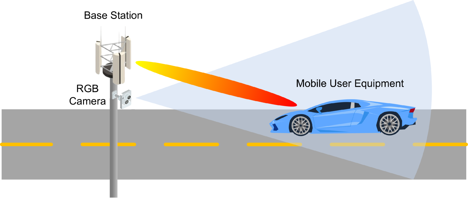
Figure 1: Illustration of the system model considered.

II System Model and Problem Formulation

II-A System Model

Fig. 1 illustrates the system model considered for vehicle-to-infrastructure (V2I) mmWave communication. In this model, the base station (BS) deploys a mmWave phased-array receiver with $M$ elements of half-wavelength spacing and an RGB camera. The antenna array enables the BS to perform beamforming, while the camera captures images within its field of view at a certain frame rate for sensing and downstream applications.

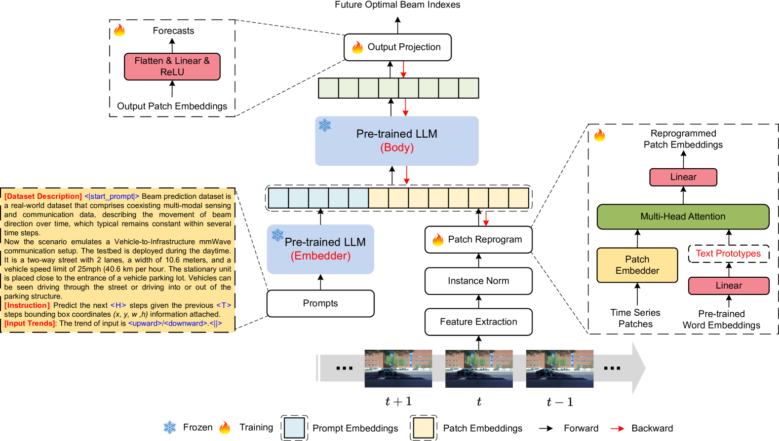
Figure 2: The model framework of BeamLLM.

We assume that the BS has a predefined beamforming codebook $\mathcal{F}=\{\mathbf{f}_{1},\cdots,\mathbf{f}_{|\mathcal{F}|}\}$, containing $|\mathcal{F}|$ beams, where $\mathbf{f}_{m}\in\mathbb{C}^{N\times 1},m=1,\cdots,M$ represents the $m$-th beamforming vector. The UE is assumed to have a single antenna. At time step $t$, the user transmits a single symbol $s[t]\in\mathbb{C}$ that satisfies the power constraint $\mathbb{E}[|s[t]|^{2}]=P$, where $P$ represents the transmit power. At the BS, the received signal $y[t]$ can be expressed as:

$$y[t]=\mathbf{h}^{H}[t]\mathbf{f}_{m}[t]s[t]+n[t],$$ (1)

where $\mathbf{h}[t]$ is the channel vector, $\mathbf{f}_{m}[t]$ is the $m$-th beamforming vector from the codebook in time step $t$, and $n[t]\sim\mathcal{CN}(0,\sigma^{2})$ is the additive white Gaussian noise (AWGN) with variance $\sigma^{2}$.

II-B Problem Formulation

This paper mainly focuses on the beam prediction problem at the BS. Given the available sensing information up to time $t-1$, the BS attempts to determine the optimal beams for $H\in\mathbb{Z}^{+}$ future time steps, specifically for $t,\cdots,(t+H-1)$. We define the optimal beam at time step $t$ as the beam that provides the highest beamforming gain, given by:

$$\mathbf{f}_{m}^{*}[t]=\arg\max_{\mathbf{f}_{m}[t]\in\mathcal{F}}|\mathbf{h}^{H}[t]\mathbf{f}_{m}[t]|^{2}.$$ (2)

When perfect CSI knowledge is unavailable, beam training serves as an alternative method for determining the optimal beam. However, with a narrow beam codebook, the training overhead can be significant, and the likelihood of identifying the optimal beam is often low when the pre-beamforming SNR is poor. Because the optimal beam selection at the transmitter and receiver depends on the surrounding environment of the transceiver, our work aims to leverage visual information at the BS to assist beam selection and develop a beam prediction framework.

III Large Laguage Model-Based Beam Prediction

In this section, we introduce BeamLLM to tackle the vision-assisted beam prediction task outlined in Section II. Fig. 2 illustrates the proposed BeamLLM. The architecture mainly comprises three components, i.e., the visual data feature extraction module and the backbone module.

III-A Visual Data Feature Extraction Module

To process raw RGB data for the vision-aided beam prediction task, we employ the YOLOv4 object detector[11]. This detector identifies potential UEs within RGB images and extracts bounding box vectors $\mathbf{b}$. For a single image $\mathbf{X}_{I}\in\mathbb{R}^{W\times H\times C}$, bounding box vector is given as:

$$\mathbf{b}=\text{YOLO}(\mathbf{X}_{I})=[x_{c},y_{c},w,h]^{T},$$ (3)

which consists of the detected object’s center coordinates ($x$-axis, $y$-axis), width, and height within the RGB image. Since the optimal beam selection is highly dependent on the direction and position of the transmission target, we use a sequence of bounding box vectors as the extracted visual feature. The objective is to predict the optimal beam index for the next $H$ steps based on the historical $T$ step bounding box vectors, denoted as $\mathbf{B}=[\mathbf{b}[t-T+1],\cdots,\mathbf{b}[t-1]]\in\mathbb{R}^{4\times T}$.

III-B The Backbone Module

The inherent potential of LLMs can be utilized to address the beam prediction task. However, a key challenge lies in aligning the visual feature modality with the textual modality to enable LLMs to effectively comprehend the task. Furthermore, fine-tuning LLMs requires extensive datasets, which is often unrealistic in practical scenarios.

Time-LLM simultaneously addresses both challenges through reprogramming[12], which consists of two key steps: adaptation and alignment. Specifically, adaptation is achieved via the patch reprogramming module, which enables LLMs to process input data effectively, thereby breaking domain isolation and facilitating knowledge sharing. Alignment, on the other hand, is accomplished through the prompt-as-prefix (PaP) module, which further eliminates domain boundaries to enhance knowledge acquisition.

Input Embedding: For each row of $\mathbf{B}$, denoted as $\mathbf{B}^{(i)}\in\mathbb{R}^{1\times T}$ for $i=1,2,3,4$, reversible instance normalization (RevIN)[13] is applied individually to normalize the data, ensuring a mean of $0$ and a variance of $1$. RevIN dynamically adjusts the normalization parameters to accommodate variations in the data distribution. Subsequently, $\mathbf{B}^{(i)}$ is segmented into several contiguous overlapping or non-overlapping patches, each of length $L_{p}$. The total number of input patches is given by $\lfloor\frac{T-L_{p}}{S}\rfloor-2$, where $S$ represents the horizontal sliding size. This operation is inspired by techniques in CV, wherein local temporal information is aggregated within each patch to better preserve local semantic features. Finally, a simple linear layer is employed to embed $\mathbf{B}^{(i)}_{P}\in\mathbb{R}^{P\times L_{p}}$ into $\hat{\mathbf{B}}^{(i)}_{P}\in\mathbb{R}^{P\times d_{m}}$.

Patch Reprogramming: Since natural language and input features belong to different modalities, with different ways of representing semantics, LLMs cannot directly process $\hat{\mathbf{B}}^{(i)}_{P}$. To address this, the reprogramming layer maps the input time sequence of visual features into an NLP task, enabling the utilization of LLMs’ reasoning and inference capabilities. A common technique for aligning different modalities is cross-attention[14], which enables interactions between word embeddings and input features by dynamically attending to relevant information across modalities. In this framework, the temporal input features serve as the query, while the word embeddings act as the key and value. However, given that the backbone model is a general-purpose LLM, the original vocabulary of size $V$ is not entirely relevant to our task. Directly aligning inputs features with all words is impractical, as many words do not carry semantic relevance to the task. Therefore, a simple linear layer is employed to extract text prototypes (semantic prototypes) by projecting pre-trained word embeddings $\mathbf{E}\in\mathbb{R}^{V\times D}$ onto a small collection of text prototypes $\mathbf{E}^{\prime}\in\mathbb{R}^{V^{\prime}\times D}$, where $V^{\prime}\ll V$. Here, $D$ is the hidden dimension of the backbone model. This projection effectively reduces the number of words from $V$ to $V^{\prime}$, allowing the temporal input features to align only with these prototypes. For each head $k={1,2,\cdots,K}$, we define:

$$\mathbf{Q}_{i}^{(k)} =\hat{\mathbf{B}}^{(i)}_{P}\mathbf{W}_{k}^{Q},$$ (4)

$$\mathbf{K}_{i}^{(k)} =\mathbf{E}^{\prime}\mathbf{W}_{k}^{K},$$ (5)

$$\mathbf{V}_{i}^{(k)} =\mathbf{E}^{\prime}\mathbf{W}_{k}^{V},$$ (6)

where $\mathbf{W}^{Q}_{k}\in\mathbb{R}^{d_{m}\times\lfloor\frac{d_{m}}{K}\rfloor}$ and $\mathbf{W}^{K}_{k},\mathbf{W}^{V}_{k}\in\mathbb{R}^{D\times\lfloor\frac{d_{m}}{K}\rfloor}$.

The following process adaptively obtains the text descriptions corresponding to patches through a multi-head self-attention mechanism:

$$\mathbf{Z}_{k}^{(i)} =\mathrm{ATTENTION}\left(\mathbf{Q}_{k}^{(i)},\mathbf{K}_{k}^{(i)},\mathbf{V}_{k}^{(i)}\right)$$

$$=\mathrm{SOFTMAX}\left(\frac{\mathbf{Q}_{k}^{(i)}{\mathbf{K}_{k}^{(i)}}^{\top}}{\sqrt{d_{k}}}\right)\mathbf{V}_{k}^{(i)}.$$ (7)

By aggregating each $\mathbf{Z}^{(i)}_{k}\in\mathbb{R}^{P\times d}$ across all heads, we obtain $\mathbf{Z}^{(i)}\in\mathbb{R}^{P\times d_{m}}$. This is then linearly projected to align the hidden dimension with the backbone model, resulting in $\mathbf{O}^{(i)}\in\mathbb{R}^{P\times D}$.

PaP: Natural language-based prompts serve as prefixes to enrich the input context and guide the transformation of reprogrammed patches. We have identified three essential components for constructing an effective prompt: (1) dataset description, (2) task description, and (3) input statistics. The dataset description offers the LLM with fundamental background information about the input features, which often exhibit distinct characteristics across different domains. The task description offers crucial guidance to the LLM for transforming patch embeddings in the context of the specific task. Additionally, we incorporate supplementary key statistics, such as trends, to further enrich the input features, facilitating pattern recognition and reasoning.

Output Projection: By packaging and forwarding the prompts along with the patch embeddings $\mathbf{O}^{(i)}$ through the frozen LLM, we discard the prefix portion and obtain the output representations. These representations are then flattened and linearly projected to produce the final outputs, $\hat{\mathbf{P}}=[\hat{\mathbf{p}}[t],\cdots,\hat{\mathbf{p}}[t+H-1]]\in\mathbb{R}^{M\times H}$. The index of the dimension corresponding to the maximum value of each $\hat{\mathbf{p}}[t]$, is predicted as the optimal future beam index, given by:

$$\hat{m}^{*}[t]=\arg\max_{m\in[1,|\mathbf{\mathcal{F}}|]}\hat{\mathbf{p}}[t].$$ (8)

III-C Learning Phase

The beam prediction task is essentially a classification problem; therefore, the model parameters are optimized by minimizing the cross-entropy, which is expressed as:

$$\mathcal{L}=\sum_{j=t}^{t+H-1}\sum_{m=1}^{|\mathbf{\mathcal{F}}|}f^{*}[j]\log_{2}(p_{m}[j]),$$ (9)

where $f^{*}_{m}[j]\in\{0,1\}^{M}$ is the $m$-th element of the one-hot encoded vector of $\mathbf{f}^{*}_{m}[j]$ and $p_{m}[j]$ is the $m$-th element of the output vector $\hat{\mathbf{p}}[j]$ at time step $j$, respectively.

IV Performance Evaluation

We utilize the DeepSense 6G dataset[15] for simulation and performance evaluation. DeepSense 6G is a multimodal dataset from real-world measurements, including wireless beam data, RGB images, GPS locations, radar, and LiDAR.

IV-A Experimental Settings

Dataset Processing: We adopt Scenario 8 of the DeepSense 6G dataset for our simulation, which simulates a V2I mmWave communication setup. The BS is equipped with an RGB camera and a $16$-element $60$ GHz mmWave phased array, while the mobile UE serves as a mmWave transmitter. During data collection, the UE passes by the BS multiple times. At each time step, the BS captures an RGB image of the UE while scanning all predefined beams and measuring the received power for all $|\mathcal{F}|=32$ beams in a codebook. The multimodal data streams are synchronized to ensure temporal consistency.

The dataset is split into $70\%$ training, $10\%$ validation, and $20\%$ test sets. The dataset consists of multiple data sequences. In each data sequence, the vehicle passes by the BS once. Each data sequence is a pair comprising an RGB image sequence and a beam index sequence. For each data sequence, we decompose it into data samples using a sliding window of size $13$. As previously mentioned, during training, we use an observation window of size $T$, and we train the model to predict future beams over a horizon $H$. Therefore, the input to the encoder for the model is ${\mathbf{X}_{I}[1],\ldots,\mathbf{X}_{I}[T]}$. In both beam prediction methods, the expected output from the decoder is ${\hat{\mathbf{p}}[T+1],\ldots,\hat{\mathbf{p}}[T+H]}$. Since we maintain a fixed sequence length of 13, we set $T=8,H=5$ as standard prediction and $T=3,H=10$ as few-shot prediction.

Baselines: We compare our approach with several classical time-series models, including RNN[1], GRU, and LSTM. Additionally, to validate the effectiveness of the PaP module, we conduct an ablation study by comparing our model with and without PaP in the standard prediction setup.

Parameter Settings: BeamLLM is configured as following: 1) A widely-used language model, i.e., GPT-$2$[16], is employed as the LLM backbone; 2) It is trained with Adam optimizer, where the batch size and initial learning rate (LR) are $16$ and $0.001$, respectively. Additionally, a multi-step LR scheduler in $1$, $5$, $10$, $15$, $20$, $25$, $30$, $40$ epochs with a decay factor of $\gamma=0.9$ is employed; 3) The training process is set to $200$ epochs. The detailed model parameters are shown in Table I.

TABLE I: Parameter Settings of Different Models

LLM		RNN, GRU, LSTM
Patch Reprogramming	Output Projection	Embedding Layer	Sequence Model
Same as [12] except $V^{\prime}=64$	Linear 1: $4\times 8$ ReLU Linear 2: $8\times 16$ ReLU Linear 3: $16\times 32$ Softmax	Linear: $4\times 32$	Layer $1-3$: $32\times 32$ Linear: $32\times 32$

Performance Metrics: Top-$K$ accuracy is a metric that quantifies the percentage of validation samples for which the best ground truth beam is among the top $K$ model predictions with the highest probability. Mathematically, it is represented as:

$$\text{Top-}K\ \text{accuracy}=\frac{1}{N_{S}}\sum_{i=1}^{N_{S}}\vmathbb{1}_{\{m_{i}\in Q_{k}\}}$$

where $N_{S}$ represents the total number of samples in the test set, $m_{i}$ denotes the index of the ground truth optimal beam for the $i$-th sample, and $Q_{k}$ is the set of indices for the top-$K$ predicted beams, sorted by the element values in $\hat{\mathbf{P}}$ for each time sample.

IV-B Standard Prediction

In Figs. 3 and 4, we present a comparative analysis of the top-$1$ and top-$3$ accuracy in the standard predictions across all models. Increasing $K$ improves top-$K$ accuracy, while as prediction horizon extends further into the future, the accuracy gradually decreases. Among the models, BeamLLM achieves the highest top-$1$ and top-$3$ accuracy scores, reaching $\mathbf{61.01\%}$ and $\mathbf{97.39\%}$, respectively. Additionally, as the number of time samples increases, the decay in the top-$K$ accuracy for the LSTM model is minimal. Specifically, the top-$1$ and top-$3$ accuracy only decrease by $\mathbf{6.03\%}$ and $\mathbf{1.65\%}$, respectively, across time samples ranging from $1$ to $5$. This smaller reduction highlights the adaptability of LSTMs, as their gating mechanism adjusts information retention and updating based on task demands.

The results of the ablation study highlight the performance differences of the BeamLLM with and without the use of PaP. The average performance gap in top-$1$ accuracy between the two models is $\mathbf{5.81\%}$, while the gap in top-$3$ accuracy is $\mathbf{3.62\%}$. When comparing these scenarios, we observe that the integration of PaP significantly improves both performance and stability, compared to simply inputting the reprogrammed patch into the frozen LLM. This underscores the effectiveness of PaP in the context of this task.

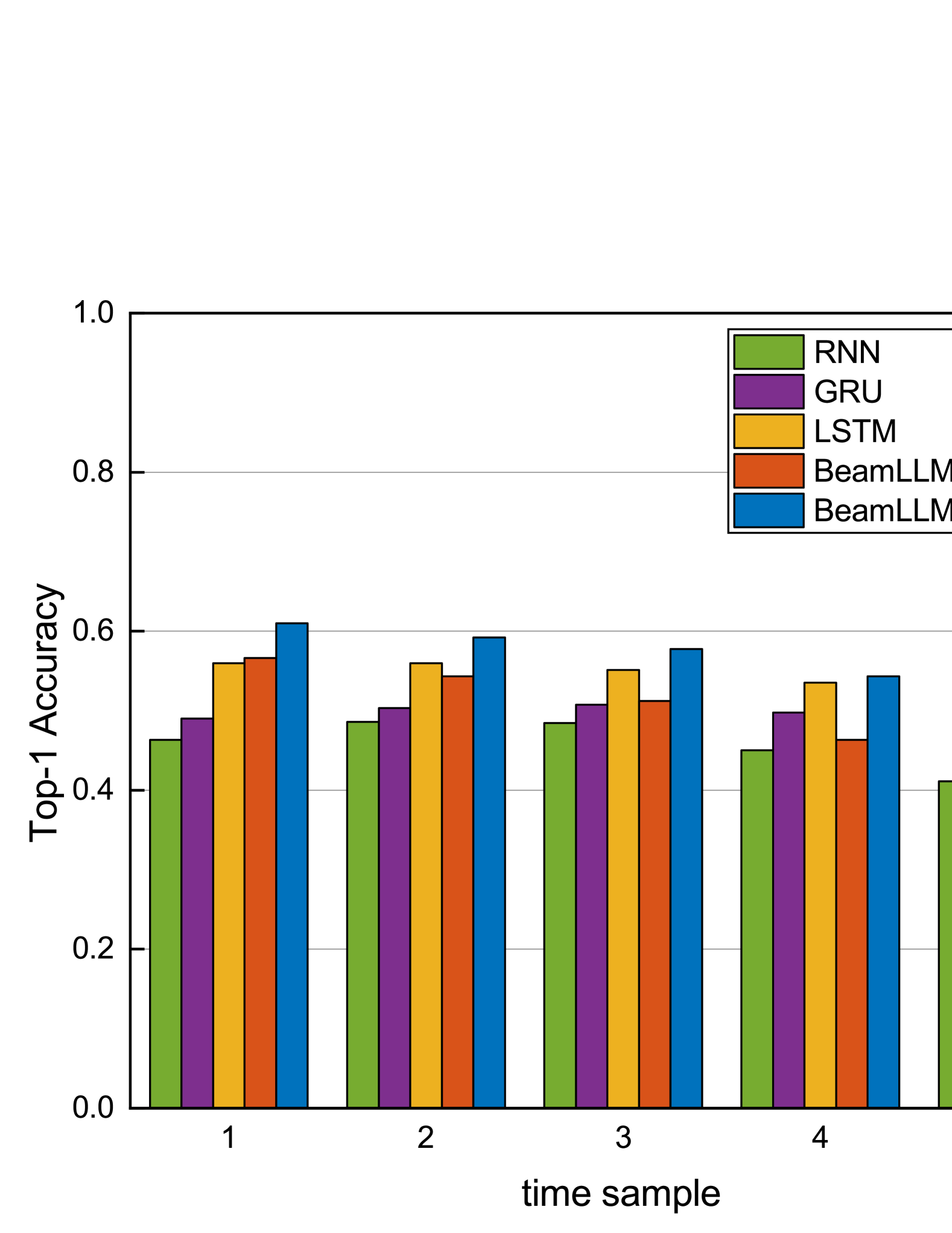
Figure 3: Top-$1$ accuracy performance of the proposed method comparing to several baselines in the standard prediction task.

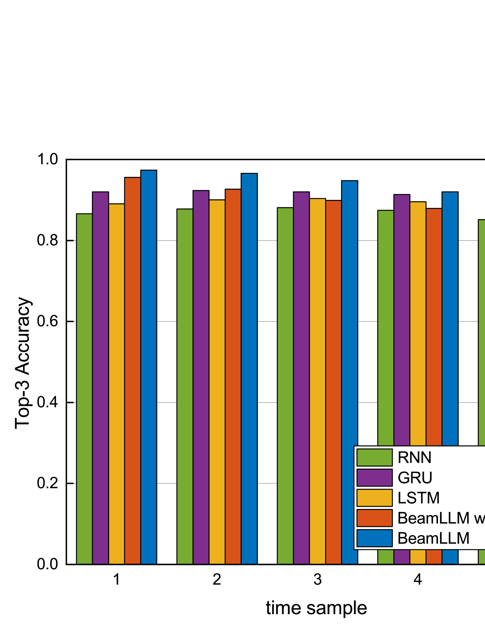
Figure 4: Top-$3$ accuracy performance of the proposed method comparing to several baselines in the standard prediction task.

IV-C Few-Shot Prediction

In Figs. 5 and 6, we present the top-$1$ and top-$3$ accuracy performance for the few-shot forecasting task. Existing DL prediction methods perform poorly in this scenario, particularly as the prediction horizon extends, resulting in severe performance degradation. Even for the previously most stable LSTM model, during the progression from time sample $1$ to 10, the top-$1$ accuracy is decreased by $\mathbf{16.48\%}$, and the top-$3$ accuracy is decreased by $\mathbf{11.58\%}$. In contrast, BeamLLM significantly outperforms all baseline methods, with only $\mathbf{12.56\%}$ and $\mathbf{5.55\%}$ performance degradation, respectively. We attribute this superior performance to the successful activation of knowledge through the reprogrammed LLM.

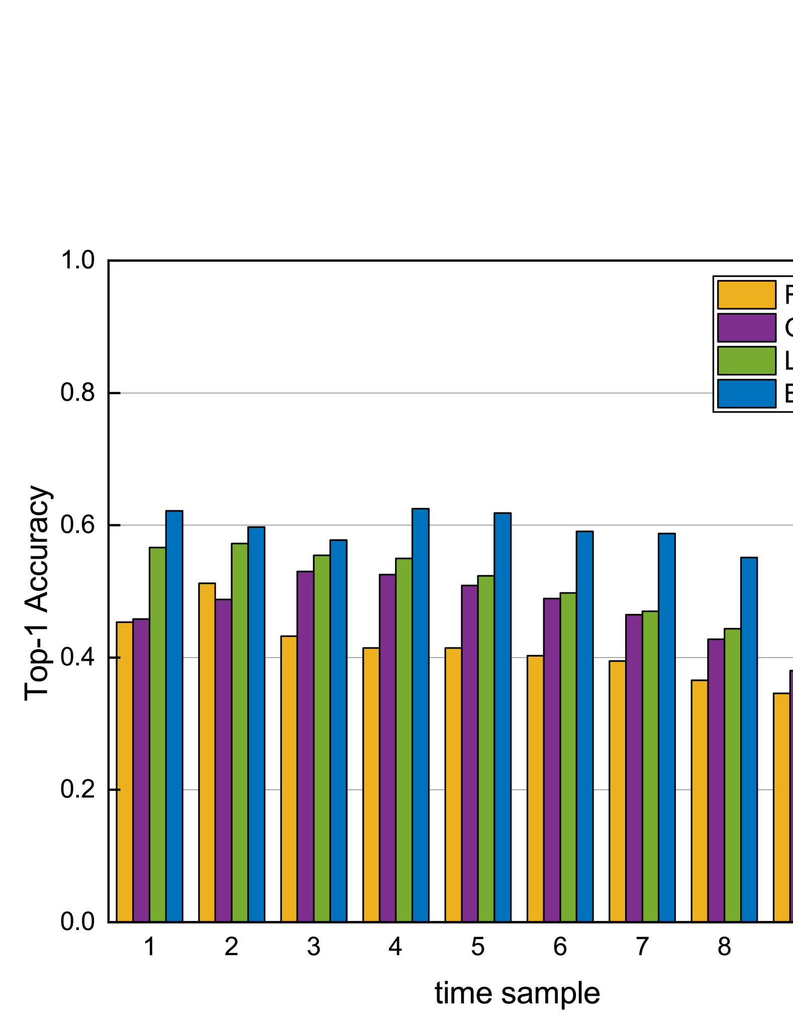
Figure 5: Top-$1$ accuracy performance of the proposed method comparing to several baselines in the few-shot prediction task.

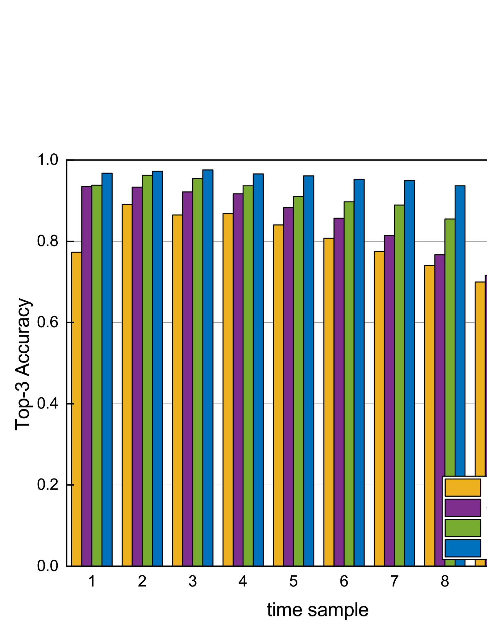
Figure 6: Top-$3$ accuracy performance of the proposed method comparing to several baselines in the few-shot prediction task.

IV-D Analysis of Reprogramming

We provide a case study of reprogramming 64 time series patches with 64 text prototypes, as shown in Fig. 7. The figure consists of three subplots, each visualizing the similarity between text prototypes computed as the scaled dot product ${\mathbf{Q}_{k}^{(i)}{\mathbf{K}_{k}^{(i)}}^{\top}}/{\sqrt{d_{k}}}$, across distinct training epochs. A color bar accompanies three subplots, with values ranging from 0 (dark purple, denoting low similarity) to 1 (bright yellow, denoting high similarity). The observed transition from a noisy, scattered pattern at epoch $1$ to a sparse and concentrated representation by epoch $5$ illustrates that the learned prototypes effectively capture the local semantic information of the input features. Moreover, the heatmaps indicate that only a few text prototypes exhibit significant correlations with the patches, suggesting BeamLLM’s ability to adaptively prioritize prototypes most relevant to the local semantic context.

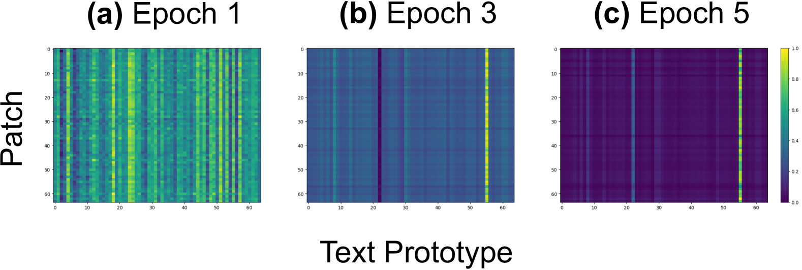
Figure 7: A showcase of text prototype evolution across training epochs.

IV-E Analysis of Complexity

All experiments are conducted in the same environment, specifically on Google Colab with an NVIDIA A$100$ GPU and $40$ GB of RAM. We investigate the training complexity and inference complexity of different models in terms of the number of trainable and non-trainable parameters, as well as the average inference time per epoch. From Table II, we observe that although the backbone model is frozen, the number of trainable parameters of BeamLLM remains large. Meanwhile, the average inference time is significantly longer than that of traditional models. While its high deployment cost poses a challenge, this also indicates that the full potential of BeamLLM has yet to be fully explored.

TABLE II: The Number of Model Parameters and Average Inference Time

Models	# of trainable parameters	# of non-trainable parameters	Average inf. time (sec)
RNN	$8,641$	$0$	$0.17$
GRU	$18,641$	$0$	$0.15$
LSTM	$26,593$	$0$	$0.25$
BeamLLM	$130,056,118$	$124,439,808$	$10.85$

V Conclusions

This work has presented an innovative BeamLLM for vision-empowered beam prediction, significantly improving accuracy and robustness in mmWave systems through reprogramming. Experimental results have highlighted LLMs’ superior contextual inference capabilities compared to conventional DL models in standard and few-shot prediction.

However, the performance gains come with increased inference complexity. The massive parameter scale of LLMs may introduce higher resource consumption and latency. Nevertheless, BeamLLM remains practical, particularly due to its exceptional few-shot prediction capability, which enables predictions over a longer horizon. Practical deployments require a trade-off between model complexity and real-time constraints, necessitating optimizations such as model compression or lightweight architecture design. By advancing these aspects, the proposed framework could serve as a scalable and efficient beam management solution for 6G ISAC systems.

References

- [1] S. Jiang and A. Alkhateeb, “Computer Vision Aided Beam Tracking in A Real-World Millimeter Wave Deployment,” in IEEE Globecom Workshops (GC Wkshps). IEEE, 2022, p. 142–147.
- [2] U. Demirhan and A. Alkhateeb, “Radar Aided 6G Beam Prediction: Deep Learning Algorithms and Real-World Demonstration,” in IEEE Wireless Communications and Networking Conference (WCNC), 2022, pp. 2655–2660.
- [3] S. Jiang, G. Charan, and A. Alkhateeb, “LiDAR Aided Future Beam Prediction in Real-World Millimeter Wave V2I Communications,” IEEE Wireless Commun. Lett., vol. 12, no. 2, pp. 212–216, 2023.
- [4] J. Morais, A. Bchboodi, H. Pezeshki, and A. Alkhateeb, “Position-Aided Beam Prediction in the Real World: How Useful GPS Locations Actually are?” in IEEE International Conference on Communications, 2023, pp. 1824–1829.
- [5] J. He, H. Wymeersch, M. Di Renzo, and M. Juntti, “Learning to Estimate RIS-Aided mmWave Channels,” IEEE Wireless Commun. Lett., vol. 11, no. 4, pp. 841–845, Apr. 2022.
- [6] OpenAI, “GPT-4 Technical Report,” arXiv preprint arXiv:2303.08774, 2024.
- [7] D. Guo, Q. Zhu, D. Yang, Z. Xie, K. Dong, W. Zhang, G. Chen, X. Bi, Y. Wu, Y. Li et al., “DeepSeek-Coder: When the Large Language Model Meets Programming–The Rise of Code Intelligence,” arXiv preprint arXiv:2401.14196, 2024.
- [8] B. Liu, X. Liu, S. Gao, X. Cheng, and L. Yang, “LLM4CP: Adapting Large Language Models for Channel Prediction,” Journal of Communications and Information Networks, vol. 9, no. 2, pp. 113–125, Jun. 2024.
- [9] Y. Sheng, K. Huang, L. Liang, P. Liu, S. Jin, and G. Y. Li, “Beam Prediction Based on Large Language Models,” IEEE Wireless Commun. Lett., pp. 1–1, 2025.
- [10] Y. Zhang, H. Yin, W. Li, E. Bjornson, and M. Debbah, “Port-LLM: A Port Prediction Method for Fluid Antenna based on Large Language Models,” arXiv preprint arXiv:2502.09857, 2025.
- [11] A. Bochkovskiy, C.-Y. Wang, and H.-Y. M. Liao, “YOLOv4: Optimal Speed and Accuracy of Object Detection,” arXiv preprint arXiv:2004.10934, 2020.
- [12] M. Jin, S. Wang, L. Ma, Z. Chu, J. Y. Zhang, X. Shi, P.-Y. Chen, Y. Liang, Y.-F. Li, S. Pan, and Q. Wen, “Time-LLM: Time series forecasting by reprogramming large language models,” in International Conference on Learning Representations (ICLR), 2024.
- [13] T. Kim, J. Kim, Y. Tae, C. Park, J.-H. Choi, and J. Choo, “Reversible Instance Normalization for Accurate Time-Series Forecasting against Distribution Shift,” in International Conference on Learning Representations (ICLR), 2021.
- [14] H. Lin, X. Cheng, X. Wu, and D. Shen, “CAT: Cross Attention in Vision Transformer,” in IEEE International Conference on Multimedia and Expo (ICME), Los Alamitos, CA, USA, Jul. 2022, pp. 1–6.
- [15] A. Alkhateeb, G. Charan, T. Osman, A. Hredzak, J. Morais, U. Demirhan, and N. Srinivas, “DeepSense 6G: A Large-Scale Real-World Multi-Modal Sensing and Communication Dataset,” IEEE Commun. Mag., vol. 61, no. 9, pp. 122–128, Sept. 2023.
- [16] A. Radford, J. Wu, R. Child, D. Luan, D. Amodei, I. Sutskever et al., “Language Models are Unsupervised Multitask Learners,” OpenAI blog, vol. 1, no. 8, p. 9, 2019.