Plane curve singularities via divides
Plane curve singularities via divides
Abstract.
Generic relative immersions of compact one-manifolds in the closed unit disk, i.e. divides, provide a powerful combinatorial framework, and allow a topological construction of fibered classical links, for which the monodromy diffeomorphism is explicitly given as a product of Dehn twists. Complex isolated plane curve singularities provide a classical fibered link, the Milnor fibration, with its Milnor monodromy, monodromy group, and vanishing cycles. This surveys puts together much of the work done on divides and their role in the topology of isolated plane curve singularities. We review two complementary approaches for constructing divides: one via embedded resolution techniques and controlled real deformations, and another via Chebyshev polynomials, which yield explicit real morsifications. A combinatorial description of the Milnor fiber is developed, leading to an explicit factorization of the geometric monodromy as a product of right-handed Dehn twists. We further explore the structure of reduction curves that arise from the Nielsen description of quasi-finite mapping classes and from iterated cabling operations on divides. The interplay between the geometric and integral homological monodromies is analyzed, with special attention to symmetries induced by complex conjugation and strong invertibility phenomena. In particular, the integral homological monodromy for isolated plane curve singularities can be computed effectively. In contrast, for complex hypersurface singularities in higher dimensions no method of computation of the integral homology monodromy is known. Connections with mapping class groups, contact and symplectic geometry, and Lefschetz fibrations are also discussed. We conclude by outlining several open problems and conjectures related to the characterization of divides among fibered links, the presentation of geometric monodromy groups, and the existence of symplectic fillings compatible with the natural fibration structures.
1. Introduction
The concept of divides (or partage in French) has become a significant tool in the study of isolated plane curve singularities and their associated monodromy groups. Introduced in the 1970s, independently by the first author [A’C75b] and Sabir Gusein-Zade [GZ74a, GZ74b], divides provided a novel combinatorial approach to understanding the topology of singularities and their deformations. Both researchers were deeply influenced by the broader developments in singularity theory initiated by John Milnor’s foundational work on the Milnor fibration [Mil68], which showed that isolated hypersurface singularities could be understood through their associated fibration structure. Divides emerged as a geometric tool that could encode the topological behavior of these singularities by associating them with fibered links in three-dimensional spaces.
The first author’s pioneering work on divides tied tightly these objects to the monodromy of singularities. His work throughout the years drew a big picture that placed these objects as an useful and novel tool to understand plane curves. In particular, he showed that a divide associated with a plane curve singularity encoded every topological piece of information associated with the plane curve singularity: the link, a model of the Milnor fiber, the geometric monodromy as a product of Dehn twists around vanishing cycles and even the reduction curves of the Nielsen-Thurston decomposition of the monodromy. This work also demonstrated that divides could serve as a bridge between knot theory and the study of singularities, particularly by offering a combinatorial framework for understanding the monodromy representation of some fibered link that share a lot of similarities with those coming from singularity theory.
In parallel, Gusein-Zade developed an alternative approach to divides, focusing on the real morsifications of singularities and using Chebyshev polynomials to generate divides for specific classes of real plane curves. This approach offered a more algebraic route, allowing the explicit construction of divides from polynomial models. Gusein-Zade’s contributions enriched the theory of divides, showing that they could be systematically constructed for a wide variety of singularities, further connecting the geometric properties of divides with algebraic invariants like Puiseux pairs and Newton polygons.
Divides also exhibit strong symplectic properties, connecting them to the study of symplectic geometry and symplectic fillings. Research into the symplectic properties of divides has led to advances in the understanding of how these objects interact with higher-dimensional spaces, further expanding their applications.
This survey explores the modern theory of divides, focusing on their combinatorial and geometric properties, as well as their applications to the study of singularities. We discuss the role of divides in generating fibered links, describe their connections to the Milnor fiber and geometric monodromy, and highlight recent advances in the symplectic and topological study of these objects. Additionally, we state and discuss some open questions, such as the broader symplectic properties of divides.
Through this work, we aim to provide a comprehensive overview of the current state of the theory of divides, demonstrating its central role in singularity theory, knot theory, and beyond. Much of the content comes directly from the classical work of the first author. Some proofs have been revisited or expanded with some details added and new detailed examples are considered. The order in which the material is told, does not necessarily respect the chronological order in which it appeared but rather an expository one.
Organization of the paper
In Sect. 2 We fix notation and introduce some basic concepts about the theory of mapping class groups and the theory of plane cruves. Among others we introduce the Nielsen-Thurston decomposition and the important concepts of geometric vanishing cycle and geometric monodromy group associated with an isolated plane curve singularity.
In Sect. 3 we give the abstract definition of divide and we associate to it a link in the three-sphere. Furthermore, in Lemma 3.2.2 we prove the existence of adapted functions (Morse functions that define the divide) for each divide.
In Sect. 4 we prove a general fibration theorem (Theorem 4.1.1): the link that we associated to each divide is a fibered link. The fibration is given by a very explicit map which can be constructed from an adapted function.
In Sect. 5 we start the study of divides coming from plane curve singularities. In particular we introduce the concept of totally real plane curve singularity and we explain two methods to produce divides for totally real plane curves. The first method, presented in Sect. 5.2, is due to the first author and relies on choosing a resolution and then perform a series of controlled perturbations of the strict transform and contractions of exceptional divisors with self intersection alternately. The second method, explained in Sect. 5.3 is due to Gusein-Zade and it relies on the fact that Chebyshev polynomials can be used to parametrize the set of Brieskorn-Pham polynomials. This fact together with an iterative technique, allows one to produce divides for any topological type of plane curve realized by a particular real model.
In Sect. 6 we describe combinatorially the Milnor fiber of the function constructed in Sect. 4. This combinatorial description is crucial in the description of the monodromy given in Sect. 7. In the first subsection we describe the monodromy as a product of right handed Dehn twists around the geometric vanishing cycles of a distinguished basis. In the second subsection we deal with special properties of the geometric monodromy associated with a plane curve singularity, more concretely we explore the property of being strongly invertible and we discuss the state of the art in higher dimensions.
In Sect. 8, we explain how one can, from a divide, to easily produce an explicit model for the Milnor fiber together with a set of geometric vanishing cycles associated with a distinguished basis. Furthermore, if the divide is produced by the previously introduced cabling technique, we explain how to visualize in this model, the reduction curves of the geometric monodromy associated with the divide.
Finally, in Sect. 9 we state a few open questions related to divides associated with plane curves together with some other properties that are not fully explored in this work.
2. Preliminary theory on mapping class groups and plane curves
We turn now our attention to the theory of mapping class groups. The purpose of this section it to collect the results on mapping class group that we use throughout the rest of the text as well as to fix notations and conventions. For more insight on this topic we refer to the book by B. Farb and D. Margalit [FM11].
2.1. Mapping class groups
Let be a compact oriented connected surface with boundary.
Definition 2.1.1.
The mapping class group of is defined as
That is, elements of are isotopy classes of oriented diffeomorphisms of that fix the boundary point-wise. Each of these classes is called a mapping class.
Relative diffeomorphisms of a surface are in fact in the same mapping class if relatively homotopic.
Next we define the basic elements that form the mapping class group: the Dehn twists.
Notation 2.1.2.
Given a simple closed curve disjoint from the boundary on an oriented surface we denote by
a right-handed Dehn twist around or its mapping class in the mapping class group of relative to its boundary. The support of is concentrated, by definition, in a tubular neighborhood of . Also, the mapping class of only depends on the isotopy class of the simple closed curve .
Now we turn to our attention to another construction, very much related to the one above, that will turn out to be very useful later on this text. We introduce the notions: minimal positive pair of Dehn twists, half twist, right half Dehn twist and left half Dehn twist.
Definition 2.1.3.
Let be an oriented surface and let be a simple closed parametrized curve on . Let be the surface obtained from the surface by cutting along the image of and by gluing back with the diffeomorphism that identifies images of opposite points of ; denote by the image of ; we call this diffeomorphism a half twist. The surfaces and are of course diffeomorphic and and are equal as sets. A minimal positive pair of Dehn twists from to is a pair of diffeomorphisms from to such that the following holds:
-
(a)
The composition is a right Dehn twist with respect to the orientation of having the curve as core. In addition holds
-
(b)
There exists a regular collar neighborhood of in such that both and coincide with the identity of outside .
-
(c)
For some volume form on which we think of as a symplectic structure, we have , and the sum of the Hofer distances ([HZ94, Chapter 5.]) to the identity of the restrictions of and to is minimal.
Minimal positive pairs of Dehn twists exist and are well defined up to isotopy. For a minimal positive pair of Dehn twists, the member is called positive or right half Dehn twist and the member is called negative or left half Dehn twist.
Nielsen-Thurston decomposition
The following decomposition result is a landmark in mapping class group theory.
Theorem 2.1.4 (See [Thu88] and Corollary 13.3 from [FM11] ).
Let be an orientation preserving homeomorphism that restricts to the identity on . Then there exists isotopic to and a collection of non-null-homotopic disjoint simple closed curves (called reduction curves) including all boundary components such that:
-
(1)
The collection of curves is invariant by , i.e. .
-
(2)
The homeomorphism restricted to the union of components of each -orbit of connected components of is isotopic either to a periodic or to a pseudo-Anosov homeomorphism.
Definition 2.1.5.
Any collection of curves satisfying 1 above is called a reduction system. That is, a collection of simple closed curves that is invariant (up to isotopy) by is a reduction system.
The decomposition given by Theorem 2.1.4 is called Nielsen-Thurston decomposition and is unique up to isotopy if the reduction system of curves is minimal by inclusion. We assume whenever necessary that the representatives of the mapping classes used in this work satisfy 1 and 2 from the previous theorem. This decomposition leads to the following definition.
Definition 2.1.6.
Let be a representative of a mapping class, we say that is pseudo-periodic if only periodic pieces appear in its Nielsen-Thurston decomposition.
Pseudo-periodic homeomorphisms are of special importance in complex singularity theory, as all geometric monodromies of holomorphic germs of functions on isolated complex surface singularities are of this kind. In particular, monodromies of isolated plane curve singularities are of this type. In general, local geometric monodromies of complex hypersurface singularities are dynamically restricted: the geometric monodromy can be realized by a distal map, which topological entropy vanishes. This shows that in the case of curve singularities the reduction of the geometric monodromy does not have pseudo-Anosov components. See also [A’C75a].
2.2. Isolated plane curve singularities
In this section we review some basic notions on plane curve singularities that are mentioned and used throughout this text.
The algebra of convergent power series is a unique factorization domain and so, up to multiplication by a unit, a series defining an isolated plane curve singularity, can be uniquely expressed as where each is an irreducible convergent power series. Each is called a branch of and if we say that is irreducible.
The Milnor fibration
In [Mil68], Milnor proved that for a holomorphic map with an isolated singularity at the origin,
is a locally trivial fibration. Here denotes a suitably small sphere and the link is defined by . If we denote by a small disk of radius centered at and by a ball of radius , it follows from Ehresmann’s fibration lemma that
| (2.2.1) |
is also a locally trivial fibration for small enough and small with respect to . In this case, we say that is a Milnor ball and that is a Milnor radius. Milnor proved in [Mil68] that these two fibrations are essentially equivalent.
The fibers of second fibration are connected compact -manifolds with non-empty boundary , and the fibers of first fibration are diffeomorphic to the interior of the fibers of second fibration which carry a complex structure.
Any fiber of these fibrations is called the Milnor fiber of . When , the second is a connected oriented compact surface with non-empty boundary. The Milnor fiber has boundary components, where is the number of branches of . Its first Betti number coincides with
and any of these quantities is called the Milnor number of and denoted by or simply by if there is no ambiguity. The topological information of a plane curve singularity is carried by the -component oriented classical link in its oriented ambient -sphere.
Puiseux pairs and intersection multiplicities
There are a lot of different ways of codifying by numerical invariants the topological information of a plane curve singularity. We cite [BK12], [Wal04] or [EN85] as standard references on this topic.
Next, we briefly recall what Puiseux pairs are, since they appear several times on this work. In particular, Puiseux pairs codify topologically uni-branch plane curve singularities. We give an axiomatic approach to this theory.
Definition 2.2.2.
A finite sequence of pairs of integers is a sequence of essential Puiseux pairs if and only if
for all .
A sequence of essential Puiseux pairs defines a family of topologically equivalent singularities. A specific member of this family is obtained from a Puiseux expansion with fractional and strictly increasing exponents
by the rule, which takes into account the ramification of ,
where runs over the roots of in the algebraic closure of the field . The coefficients of the polynomial are integers.
For example, the Puiseux expansion with strictly increasing exponents for leads to the polynomial and the Puiseux expansion to the polynomial .
There is a second equivalent set of numerical invariants that are more suitable for certain matters: Newton pairs. These are a finite sequence of coprime integers that can be computed from the Puiseux pairs by the recursive formula
| (2.2.3) |
Instead of using the above Puiseux expansion one uses for given Newton pairs Newton’s Ansatz
which expands to the corresponding Puiseux expansion.
Now suppose that is the factorization of a reducible isolated singularity in branches . In this case, Puiseux or Newton pairs of each of the branches are not enough to determine the topology of the singularity. One need one extra piece of information, for example intersection multiplicities. For each pair , we define the intersection multiplicity between the branches and as
which is in fact the linking number of the oriented knots corresponding to these branches. For an interpretation of the numbers of eq. 2.2.3 in terms of intersection numbers, see Sect. 5.3.
For instance, Puiseux pairs and Newton pairs can be truncated: denote by or the initial entries of given equivalent and let define a sequence of plain curve singularities. Here, will be the empty set of Puiseux pairs, Newton pairs corresponding to . The equations define oriented knots . The Newton pairs get a topological interpretation: The knot is the cable knot on the knot . See the book by David Eisenbud and Walter Neumann [EN85] for references and historical remarks.
2.3. The versal deformation space and the geometric monodromy group
The versal unfolding
We briefly recall here the notion of the versal unfolding of an isolated singularity; see [AGZV88, Chapter 3] for more details. Recall the algebra
Let
be polynomials that project to a basis of , assume (we can always do so) that . For , define the function by
The base space of the versal unfolding of is the parameter space of all which is naturally isomorphic to . The discriminant locus is the subset
It can be shown that Disc is an algebraic hypersurface. The discriminant locus admits different stratifications; for example, it is stratified according to the sum of the Milnor numbers of the singular points of the singular fibers lying above. In this sense, the top-dimensional stratum (that is, the smooth part of Disc) parameterizes curves with a single node. Denote by a small closed ball in centered at the origin. Define
| (2.3.1) |
Then, for small enough and after intersecting with a sufficiently small closed polydisk, this family has the structure of a smooth surface bundle with base and fibers diffeomorphic to the Milnor fiber of eq. 2.2.1. We fix a point in and we denote, also by , the fiber with boundary lying over it.
The geometric monodromy group
Recall that a mapping class (Definition 2.1.1) is an isotopy class of orientation preserving diffeomorphisms of that restricts to the identity on the boundary, where the isotopies are required to fix the boundary point-wise. Let define an isolated singularity at the origin, with Milnor fiber .
Definition 2.3.2.
The geometric monodromy group is the image in of the monodromy representation
of the universal family of eq. 2.3.1.
Definition 2.3.3.
A quadratic vanishing cycle or geometric vanishing cycle or, for the purposes of this work, simply a vanishing cycle is a simple closed curve that gets contracted to a point when transported to the nodal curve lying over a smooth point of the discriminant Disc.
Let be a Milnor ball for an isolated plane curve singularity . Then, for any linear form generic with respect to and small enough, the map
only has Morse-type singularities and the corresponding critical values are all distinct and close to . The holomorphic map is usually called a morsification of .
Remark 2.3.4.
Two isolated plane curve singularities with the same topological type can be connected by a -parameter -constant family and thus, they have the same geometric monodromy group. This last statement follows from the following: in [GZ74a, Theorem 3] it is proven that two plane curve singularities with the same topological type can be joined by a -constant family or, equivalently, by family of singularities with the same topological type. As a consequence, the intersection matrices (of distinguished basis) of these singularities coincide. Also, by a result of Hamm and Lê [HT73], the geometric monodromy group o a plane curve singularity can be computed from any morsification. As a consequence of this discussion, the geometric monodromy group (Definition 2.3.2) of an isolated plane curve singularity is a topological invariant.
3. Definition of divide and some combinatorial properties
In this section we give the first definitions and properties of divides. In particular, we prove the existence of adapted functions to divides (Lemma 3.2.2) which are Morse functions with very particular properties.
3.1. Definition of divide
We start with the definition of the central object of this work.
Definition 3.1.1.
A divide is a generic relative immersion of a compact -dimensional manifold into a disk . Usually is a disk in the Euclidean plane or the Gaussian plane .
Notation 3.1.2.
A divide is usually identified with the image of the immersion and denoted by , that is, with the notation of the above definition .
Remark 3.1.3.
-
•
relative means that and .
-
•
generic means that the restriction of to is injective, that is transverse to , and that the curve has only ordinary double points in the interior of (this leads to the following Definition 3.1.4)
-
•
When not important, the radius of the disk will not be specified. If we need to specify the radius of the disk, we will write for a disk of radius centered at the origin.
-
•
In certain parts of this survey, we only consider divides which are immersions of disjoint union of segments and, in other parts, we also consider divides which are immersions of disjoint union of segments and circles. It will be pointed out when necessary. If no clarification is made, we assume the second and more general version.
It will be very useful to deal with a more relaxed version of the notion of divide which is one where we allow ordinary singularities other than double points.
Definition 3.1.4.
A pre-divide is a relative immersion that is generic near as above and such that for all distinct with the images of the tangent spaces
in .
Note that the only difference between a divide and a pre-divide is that in a pre-divide we admit singularities which are multiple crossing points (see Fig. 3.1.1).

We need to prepare the construction of a classical link in the
-sphere from a divide. Let be a disk (for convenience centered at
the origin) of radius in the Euclidean plane with norm
. We equip the tangent space
with the Euclidean norm
, where we denote the tangent
vector by . The -ball of radius
over is the subset in defined by
. The -sphere that will contain the
link is the boundary . Observe that
is identified with the set of tangent vectors
. Let be a divide or pre-divide in
. We denote by the set of all vectors with or
that are tangent to one of the branches of
.
In view of the study of complex plane curve
singularities, we think
as the complex plane via the identification
and choose to orient by the “complex” orientation given by the frame . As a consequence, the -ball and its boundary inherit orientations. Also the smooth part of becomes an oriented surface.
With this setting we are ready to define the link associated to a given divide.
Definition 3.1.5.
Given a divide we define the associated link as
| (3.1.6) |
We will later see that not all links come from divides. We will also see that links that come from divides are fibered and that, even not all fibered links come from divides. For example, in 7.2.8, it is explained why the figure eight knot (Fig. 3.1.2) cannot appear as the knot associated to a divide.

The projection restricts to a map having a circle as preimage of non boundary points of . Those preimages shrink to circles of radius as the point moves to the boundary. The restriction to is generically over the smooth points of not in and above . It is over the double points of .
As example, let define a divide in the disk with end points on . The divide is also defined by . The knot is the union of two oriented arcs on , one running from to , the other running from to . The first arc, using is parametrized by
The second arc, similarly, uses . Both oriented arcs fit together as an oriented knot.
A variant is following construction: First extend to an immersion of a rectangular thickening of the interval . Next, for small , restrict to a rectangle where means that we smooth the corners. Let be the boundary of with any chosen orientation. The restriction is a generic immersion of an oriented copy of into . The lifting of the oriented speed vector of yields an oriented knot which is isotopic to the oriented knot . So knots coming from generic immersed intervals, come also from generically immersed oriented circles. William Gibson and Masaharu Ishikawa [GI02] have proven that every oriented knot can be obtained by lifting a immersion of an oriented circle in .
Naturally, a small perturbation of a divide, produces an isotopic links in . We can if necessary make a divide by a small isotopy more “Euclidean friendly” without changing its link: for instance we may assume without restricting generality that the divide is near its double points an orthogonal intersection of segments. Furthermore, we can consider more involved (and no longer necessarily small) perturbations that still produce isotopic links. This leads to the following definition and lemma.
Definition 3.1.7.
We say that an isotopy of a divide is admissible if it is generated by Reidermeister moves of type only. See Fig. 3.1.3.

Lemma 3.1.8.
If and are related by an admissible isotopy, then and are isotopic in .
Proof.
Example 3.1.9.
Note that admissible isotopies do not yield a complete set of moves to go from one divide to another one with . Indeed it can be verified that the links from the figure yield isotopic knots but one cannot go from one to another only admissible isotopies, see Gibson-Ishikawa, two divides for knot not related by III-moves.
Knots or links for divides are very special. For instance let be the knot of a divide . The symmetry given by the involution fixes point-wise and preserves globally, with two fixed point on . So the knot is strongly invertible, see Makoto Sakuma [Sak86]. Divides links are closures of quasi positive braids by Tomomi Kawamura’s result [Kaw02].

3.2. Adapted Morse function on and its extension on
Definition 3.2.1.
Let be a divide. We say that a smooth function
is adapted to if
-
(1)
is locally generic, i.e. it only has non-degenerate critical points
-
(2)
each bounded region has exactly one non-degenerate maximum or minimum. in its interior with critical values
-
(3)
the saddle points of are exactly at the double points of and .
-
(4)
each contractible unbounded region has exactly one non-degenerate maximum or minimum on its intersection with .
-
(5)
if then the restriction of to is constantly .
Note that is a Morse function in a disk slightly bigger than where we allow different critical points to have the same critical values.
Lemma 3.2.2.
Let be a connected divide. Then there exist adapted functions .
Proof.
We may change the divide by a small
isotopy in order to make it “Euclidean friendly”, i.e. at its double
points
will consist of a pair of Euclidean orthogonal segments. Every
connected component of , that we also call region, does not
meet or meets in a connected set since by
hypothesis is connected. We mark each such connected set by one point
if it is a contractible arc in the boundary of .
We color the regions by signs and in a chequerboard way, i.e. two
regions separated by a subinterval in will have opposite signs. This
is possible since is simply connected and as planar graph has only
vertices of valency . Next, we mark each region that not meets the
boundary of with a point. Let be a real such that the Euclidean
balls of radius in with center a marked point are
disjoint from , from if its center is not on ,
and from each other. Assume also that the intersection of with a ball
of radius and center a double point of is the union of two
Euclidean segments. We denote by the ball of radius with center
a marked point or double point of .
Now we can construct the function . Define at a marked point
or double point of to be standard Euclidean expression defining a
local maximum, local minimum, or saddle point according sign or to be a
double point of . So on define if is in a
region, or where are
local signed linear equations of Euclidean norm for the segments of
at . For a marker point we define on
as a norm linear boundary maximum or minimum with value or . If
does not meet we define
according the sign of the adjacent region. Finally put for . The so partially defined function extends in a up to isotopy unique way
to a smooth function that has no singularities except
at the marked points and double points of .
∎
Let be a non negative smooth bump function
that evaluates to for and to for . Let be the smooth function that evaluates to on the complement
of the union and to
.
We define a complex function
that depends on a real small parameter by
| (3.2.3) |
The function satisfies the Cauchy-Riemann equation at points in and points in -balls of radius in and center a Morse critical point of . These properties help to prove in next section a fibration theorem and compute the geometric monodromy, mainly following pioneering work of Milnor and Brieskorn.
More precisely, the argument function defines on an oriented open book structure with smooth binding like the argument function does on the Milnor sphere of an isolated hypersurface singularity . More over behaves like a morsification of the singularity , which allows a computation of the monodromy of that open book following:
4. General fibration theorem
4.1. A connected divide yields a fibered link
A main results from [A’C98a] about divides is:
Theorem 4.1.1.
Let be a connected divide. For and sufficiently small, the map induces an oriented open book decomposition of with binding , that is:
-
(1)
is a fibration of the complement of over ,
-
(2)
For all , the boundary of each fiber (page of the open book) is the binding, i.e.,
Proof.
There exists a regular product tubular neighborhood of such that the map for any is on a fibration over , for which near the fibers look like the pages of a book near its back. It is crucial to observe that in the intersection of the link with the support of the function
the kernel of the Hessian of and the kernel of the differential of the map
coincide. For an alternative proof of this step, look at 7.1.3 and the discussion before.
For any , the map is regular at each point of were is a small neighborhood of the critical points of . Take now local real coordinates around a maximum so that and . In these coordinates, seeing , we have that looks like
and
Let be a point in that projects to . Then, the differential of evaluated at that point equals:
and the two non-zero entries of the matrix can’t be at the same time for a point of the form since . This shows that the jacobian of has rank on those points and hence, is a submersion on a neighborhood . The computations for a minimum or a saddle point are very similar.
Finally, since the norm of the derivative of can be bounded, a similar computation yields that there exists such that for any with , the map is regular on Hence, for sufficiently small the map is a submersion, so since already a fibration near it is a fibration by Ehresmann fibration theorem.
∎
5. Divides for plane curve singularities
In this section we construct a divide associated to a given isolated plane curve singularity in the sense that is a model for the link of the plane curve sngularity. What we actually produce is a real morsification of a totally real plane curve singularity; and this real morsification yields a divide. We do so, following two different programs: the first one Sect. 5.2 gives an algorithm to construct such a divide from an embedded resolution of the plane curve, the second one, in Sect. 5.3 gives a closed formula that produces a divide from a complete set of topological invariants of a plane curve.
5.1. Totally real models of plane curve singularities
For both methods, it is necessary to start with a totally real model of our isolated plane curve singularity.
Definition 5.1.1.
Let be a converging power series and let be a factorization into irreducible factors. We say that is real or that it defines a real plane curve singularity if it is given by a real equation, that is, if . We say that is totally real if for all .
Equivalently, is real if the curve is invariant under complex conjugation and is totally real if each of its branches is real.
Once one has a real plane curve singularity, one can try to perturb it in a controlled way with the hope that all the critical points (as a complex function) are actually real and as simple as possible: Morse. It turns out that if one is able to do this, the real picture picture of the deformed curve tells us a lot about the complex singularity. Actually, this contains all the topological information of the plane curve singularity. In particular one is able to recover a distinguished basis of geometric vanishing cycles. These special types of deformations are called real morsifications:
Definition 5.1.2.
Let define an isolated real plane curve singularity, let be a Milnor ball for and let be a Milnor disk for . We say that a family of convergent power series is a real morsification of if
-
(1)
it is a deformation of , that is, ,
-
(2)
is real for all ,
-
(3)
for all the map only has Morse critical points and they all lie in . Furtheremore, the number of Morse critical points does not depend on .
-
(4)
all its critical points are real, that is, they lie in .
-
(5)
all saddle points lie over .
In the next two sections we prove, in two different ways, that there exist real morsifications for totally real isolated plane curve singularities. It is still an open question if there exist real morsifications for all isolated real plane curve singularities. See [LS18] for a partial solution to this question and see [FPST22] for the implications of a solution of this problem in other conjectures.
Remark 5.1.3.
It follows from the topological classification of isolated plane curve singularities that, given a topological type, it is always possible to find a totally real isolated plane curve singularity realising that topological type (see [Zar65a, Zar65b, Zar68] for a classical reference or [Wal04, Corollary 5.3.3 and Lemma 2.3.1] for a more recent and concrete reference). See also the previous related 2.3.4
5.2. Divides from an embedded resolution
In this section we reproduce the proof of one of the main results (Théorème 1.) from [A’C75b] which proves the existence of divides for plane curve singularities. More concretely, the proof gives an algorithm to construct a polynomial real deformation of a plane curve singularity under the hypothesis that the singularity is given by a totally real polynomial.
Theorem 5.2.1.
Let be a totally real polynomial defining an isolated plane curve singularity. Then there exists a real polynomial deformation , such that and that for all and small enough, we have
-
(1)
the real curve is a divide with branches in a small disk near the origin.
-
(2)
the number of double points of verifies , where is the Milnor number of at .
Next we explain the main construction on which its based the proof of Theorem 5.2.1 which consists in iteratively blowing up until, exactly, the strict transform is resolved and consists of smooth branches meeting transversely (but not in normal crossings) the exceptional divisor. At this point, we translate slightly the strict transforms along some exceptional divisor and blow-down back all the exceptional divisors, proving that the translation yields a deformation of the original plane curve in . Performing this operation as many times as necessary, yields a pre-divide (recall Definition 3.1.4) which can be further polynomially deformed into an actual divide.
Next we explain this process in more detail. Let be a totally real polynomial defining an isolated plane curve singularity . Let
be a sequence of transformations that yield an embedded resolution of , where
-
(1)
-
(2)
is the blow-up at the origin.
-
(3)
for is a blow-up at a point in the exceptional divisor of
-
(4)
is a union of pairwise transversal smooth curves.
-
(5)
is a composition of blow ups that resolves all the ordinary singularities of where two or more components of the strict transform of meet
-
(6)
is a hypersurface in having as singularities only normal crossings.
In other words, is an usual sequence of blow ups of the minimal resolution of the plane curve defined by just until the strict transform consists of smooth curves not meeting in normal crossings, and is the composition of all the remaining blow ups that give an embedded resolution of the plane curve.
For , we denote by
the total transform in , by
the exceptional divisor in , and by the component of , which is the exceptional divisor corresponding to the blow-up .
Let be a homogeneous coordinate system on such that the affine chart contains the intersection points of with the other branches of . Let be a chart of such that we have and with the multiplicity of in .
Since is totally real by hypothesis, we can choose the blow-ups for having as center a real point of . So we can also choose the coordinates and to be real at each step of the resolution process. The function
is written in the chart like
We decompose with the initial homogeneous part. Assume that , with , is the component of that intersects . Then, is of degree . So the set
is the union of the tangents to the non-exceptional branches of at the points of . For we put
where are the roots of . For and small enough, the equation
has exactly distinct roots on (and not in ) and
We can see in Fig. 5.2.1 the branches of that cross and .

For real, non-zero and small, Fig. 5.2.2 is the actual real drawing of

Neighbouring points on the branch are translated out and next to . So meets in normal crossings. The presence of the factor in allows us to push the function to a function on . We observe that by construction,
and for real and small enough, the hypersurface
has in the singularities:
-
a)
an isolated singularity in ,
-
b)
if are the translates of neighbouring points on ; then has at points
isolated ordinary singularities. That is, transversal intersections of smooth branches.
The blow-ups resolve the singularity at of so that the branches of - meet each other transversely. We can therefore start the construction again and obtain a deformation of .
such that the hypersurface has an isolated singularity in . In addition, one must take care so that
at a high enough order at the points . This operation can be iterated times to obtain a family of functions on .
We finally define
From this construction, the following lemma follows:
Lemma 5.2.2.
For and small enough, the curve is an immersion such that
-
a)
The number of components of equals the number of branches of ,
-
b)
, and the set is connected.
-
c)
has as as its only singularities, ordinary singularities.
In particular, b) and c) say that is a connected pre-divide (recall Definition 3.1.4).
The number of double points appearing near a multiple point with branches of , is
So the number of double points of any divide next to is
| (5.2.3) |
In the next theorem we complete the proof of Theorem 5.2.1, by proving that can be polynomially perturbed into a divide and we also show that the invariant of the singularity coincides with the number of double points of any divide coming from a totally real singularity is we only need to prove.
Lemma 5.2.4.
Let be a divide resulting from a small perturbation of . Then there exists a real polynomial so that the function
is a deformation of , such that its divide has the configuration of the divide defined by and is close to the image of .
Moreover, if are the crossing points (ordinary singularities) of , and is the number of branches of at points . Then we have
Equivalently, the number of double points of the divide coincides with the invariant of the singularity and
Proof.
Let the crossing points (double or multiple) of of . Assume that is a multiple crossing point since if there are only double points, the lemma is proven because our deformation is given by a polynomial.
Let be the number of branches at the point . Let, for ,
the equations of the tangents at to the branches of . Any configuration of a divide which is close to can be described near by an equation
where . Thus, the equation
| (5.2.5) |
gives for and small enough the same configuration. Let let be the double points that appear near for the equation eq. 5.2.5. Let be a polynomial such that for a high enough order we have
Then
is a deformation of such that the curve
has near the desired configuration and , are still multiple points of . Repeat the same construction for another multiple crossing point until there are no more. This proves the first part of the statement.

The second part follows from the following observation: if one has an ordinary real singularity consisting of branches, after a small perturbation of these branches, there appear double points (Fig. 5.2.3). Let’s denote
the number of double points of the divide. We first recall Milnor’s formula [Mil68] relating the Milnor number , the delta invariant and the number of branches . Let be the number of bounded regions of the divide. Since on each bounded region there lies a critical point of and all the other critical points are the nodes of the divide, we have
| (5.2.6) |
The connectedness of the divide implies that the union of the closure of the bounded regions is a topological disk, hence a direct calculation of the Euler characteristic yields
| (5.2.7) |
Taking eq. 5.2.6 minus eq. 5.2.7 yields which, after Milnor’s formula implies . ∎
Example 5.2.8.
This is an example of a divide using a similar technique as the one explained in Theorem 5.2.1. Note that the perturbations chosen here are not exactly the same.
Start with the isolated plane curve singularity defined by the polynomial .
After four blow ups we arrive at the situation of Fig. 5.2.4. In a local chart, near the intersection point of the divisors and , the total transform is defined by the expression
We can perturb the strict transform by considering the polyomial :
which, for defines the picture of Fig. 5.2.5.
Now, we observe that the contraction of , yields the equation
which, for describes the situation depicted in Fig. 5.2.6
Again, we perturb the strict transform in order to achive normal crossings by considering the following polynomial
We arrive to the situation of
To avoid cumbersome notation, we have used the same parameter for the perturbation. One can think of this as two steps: first one considers a perturbation over a two-parameter family; then one considers the perturbation over a disk contain in this family. By the choice of our pertubations, we are considering the pertubation over the diagonal of this two-parameter family. Note that Theorem 5.2.1 proposes, a priori different pertubations to ensure that they behave well with respect to the blow-down process. In our case, we verify this at each step even though we make different choices that the ones proposed by the theorem. In the above equation, defines locally and defines . After the contraction of we arrive to the polynomial
which, for defines the situation depicted in Fig. 5.2.8.
In this case, the strict transform already intersects the divisor transversely. So we don’t perform a perturbation at this stage and we directly contract to arrive to the equation
which describes the local situation depicted at Fig. 5.2.9.
As we see, the (perturbed) strict transform does not meet in normal crossings the divisor . So we need to perturb it a little bit. We do so by considering the polynomial
which results from substituting by in the strict transform of the equation defined by . For the corresponding situation is depicted in Fig. 5.2.10.
We are ready to contract the divisor to arrive to the polynomial
This is already a polynomial defined in the (original) that is a deformation of and that defines a pre-divide (recall Definition 3.1.4) which is depicted in Fig. 5.2.11.
After performing a generic pertubation as explained in Lemma 5.2.4 we arrive at a divide like the one in Fig. 5.2.12 which is a divide for our original singularity.

5.3. Divides from Chebyshev polynomials
In this section we explain a different way to obtain divides for plane curves. This was envisaged by Sabir Gusein-Zade in [GZ74b, GZ74a] and was also further explored by the first author.
It was observed by René Thom that the Chebyshev polynomials up to affine equivalence of functions are precisely the polynomial mappings from to with two or less critical values and with only quadratic singularities [Tho65]. The standard Chebyshev polynomial is a polynomial in the variable of degree and has the following properties:
-
(1)
its critical are values ,
-
(2)
it has the symmetry , and
-
(3)
the coefficient of is .
As a consequence of these properties we find that, for example, the map has no critical values and the map has only the critical value . Furthermore, the Chebyshev polynomial satisfies the identity
and its restriction to is defined by
Sabir Gusein-Zade [GZ74b, GZ74a] constructed real morsifications for real plane curve singularities with Chebyshev polynomials. The building block for his construction is the real morsification for the map given by
In particular, it is a direct computation that for each , the function has quadratic singularities all at points with real coordinates, its critical values are contained in and
If the exponents and are relatively prime to each other, the level set can be parametrized by the monomial map
The Chebyshev composition identity (see [Riv74])
implies that in this case, the Chebyshev polynomials can also be used to parametrize the level sets as well. Indeed, the map
parametrizes the level set . Equivalently, one can verify that
| (5.3.1) |
Gusein-Zade method
As a consequence of this, Gussein-Zade [GZ74a] showed that if
is a parametrization of a branch with , then
| (5.3.2) |
defines, for , a divide for that branch. Observe that any real branch admits a real parametrization.
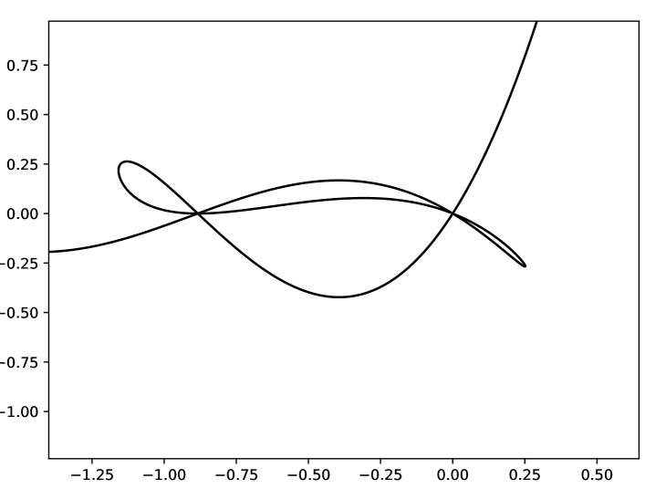
Example 5.3.3.
We compare now this method with the method described in the previous Sect. 5.2. In particular, we consider the plane curve singularity defined by the polynomial
which is the one used in Example 5.2.8. A direct computation yields that the map
is a parametrization of the branch near the origin. And so the formula eq. 5.3.2, yields that the following describes a divide for each :
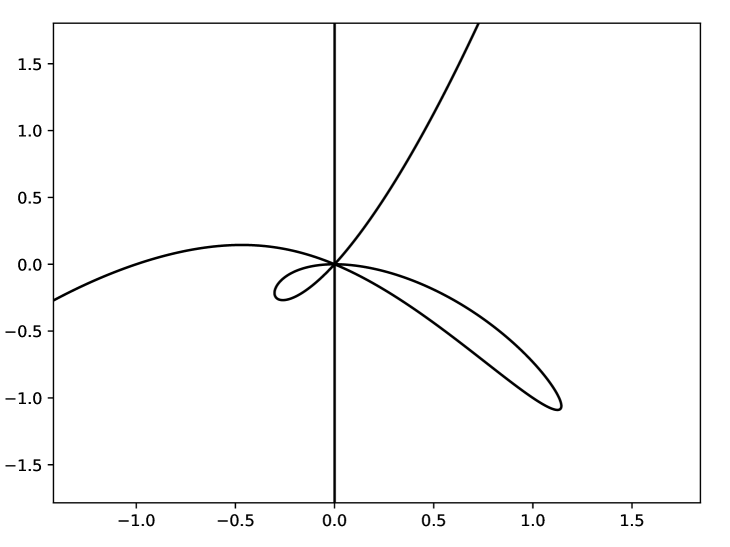
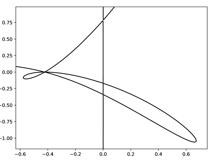
Where the equality is just the evaluation of the Chebyshev polynomials and simplification of the expressions. For we obtain the divide depicted in Fig. 5.3.1. Compare with that of Fig. 5.2.12
It follows from the defining property that the curve defined by the above parametrization has
| (5.3.4) |
double points near the origin. Since has critical points (all of them Morse), we have proven that the previous parametrization yields a divide. More concretely, for each the intersection
is a divide for the Brieskorn-Pham singularity defined by the polynomial at . The curve can be drawn in a rectangular box as in Fig. 5.3.2. As a first type of building block we will need the box with the curve . If holds, the curve is the image of
which leaves the box through the corners. In general, the immersed curve has several components, which are immersions of the interval or of the circle. At most two components are immersions of the interval, which leave the box through the corners.
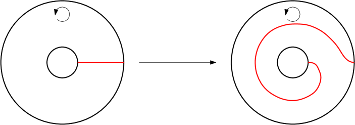
Cabling divides
Let be any divide having one branch given by an immersion . We assume, that the speed vector and the position vector are proportional at , i.e. the divide meets at right angles. Let
be an immersion of a rectangular box around , that is, the restriction
is the immersion and the image of is in a small tubular neighborhood of . For instance, for a small value of the parameter the following expression defines such an immersion of the rectangular box :
where is the rotation of over , equivalently, is multiplication by if we see the divide as a subset of . The four corners are on the circle of radius We finally define
that is an immersion mapping the corners of the box into .
Definition 5.3.5.
Let be a divide and let be two natural numbers with , we denote by
the divide in , which is the image by of . We call the -iterated divide around .
Note that by definition, an iterated -composition of divides has to be evaluated from the right to the left.
The number of double points of is computed inductively from the number of double points of by:
| (5.3.6) |
Indeed, observe that the divide has:
-
(1)
By construction, at least as many crossings as had (recall eq. 5.3.4), and hence the first summand.
-
(2)
Near each intersection point of , there appear after the cabling operation, lines crosssing with other lines, and hence the second summand.
Let be the union of the image of with the two chordal caps at the endpoints of . One can think of as a thick version of . The connected components of correspond via inclusion to the connected components of . We declare a connected component of to be signed by , if the component contains a component of , that corresponds to a component of . In this case we call the connected component of a -component. Observe that there exists a chess board sign distribution for the components of that makes -components indeed to components.
The field of cones on the box is the subset in the tangent space of given by:
where and where is a function, such that for every with and we have the equality
Moreover, has the boundary values and . We interpolate the function on by upper and lower convexity, i.e such that and . The definition of seems to be conflicting at the double points of the curve ; at a double point of the curve the two tangents lines to have opposite slopes and , since the curve is defined by the equation
that separates the variables. For example, a nice such function is given by:
The interest of the field comes from the following lemma, that follows from the definitions.
Lemma 5.3.7.
Let the image of be a divide , that meets at right angles. For small enough, the intersection of with the image in of the field of sectors under the differential of is a tubular neighborhood of the knot . The composition of and of is again a divide, whose knot is a torus cable knot of type of the knot .
The image of the field of sectors of under the differential of will be denoted by and for small contains those vectors, that have feet near and form a small angle with the tangent vectors of the divide .
Divides for plane branches
Let be a singularity having one branch and with essential Puiseux pairs (recall Sect. 2.2) . The theorem of S. Gusein-Zade [GZ74b] very efficiently describes a divide for the singularity in a closed form, namely the iteratively composed divide
where the numbers can be computed recursively, as we will show here below. We denote by the divide
and let be a specific equation for a singularity with essential Puiseux pairs .
Remember, that the product is the multiplicity at of the curve and that the linking number of and in can be computed recursively by:
The linking number is equal to the intersection multiplicity
at of the curves and (recall the definition of Newton pairs eq. 2.2.3). We have also for the linking number an interpretation in terms of divides (see the next section for the first equality) which leads to the definition of the numbers :
Remembering, that we already have computed recursively the numbers and , we conclude that too can be computed recursively.
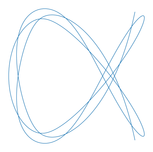
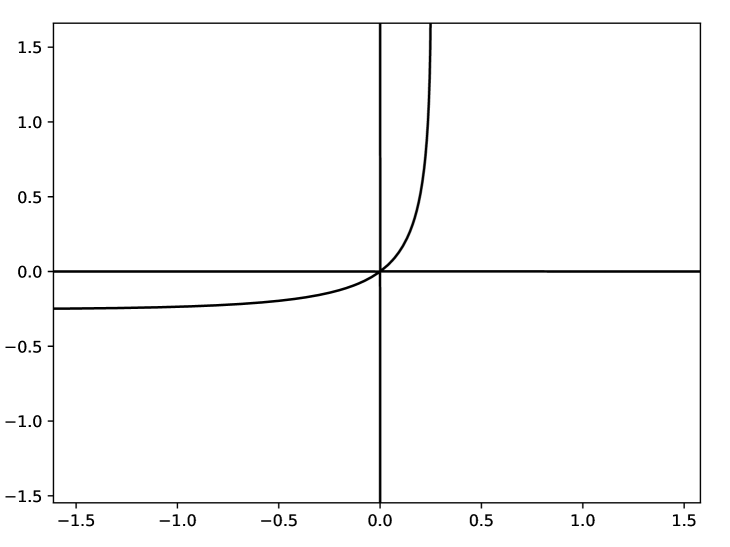
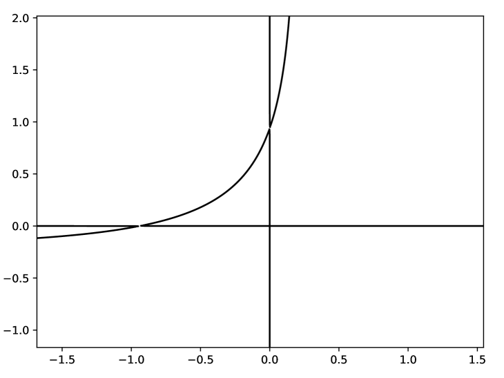
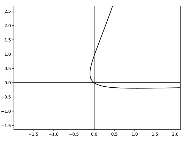
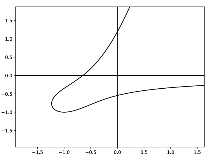
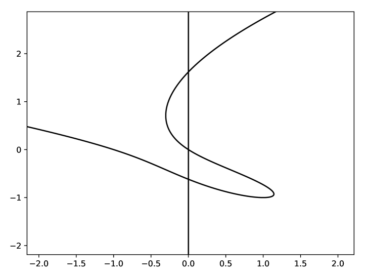
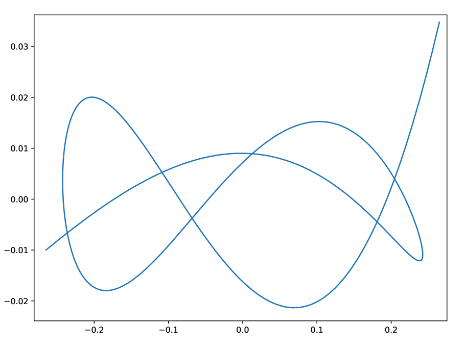
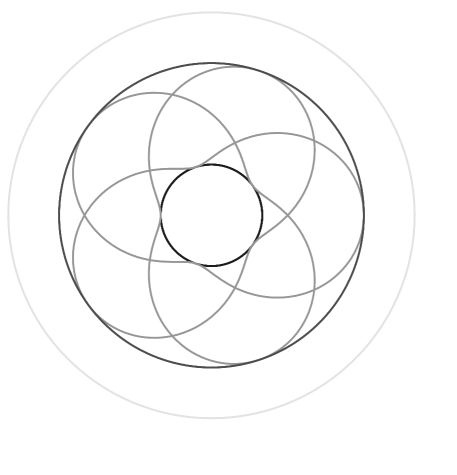
For example, for the Puiseux expansion we have: . Hence, the divide for the irreducible singularity with Puiseux expansion is the divide , see Fig. 5.3.3. For the Puiseux expansion we found: . Hence, the divide for its singularity is , see Fig. 5.3.4.
Using the contents of the (independent) Sect. 8 (c.f. [A’C99, A’C98a]), we can read off from this divide the Milnor fibration of the singularity . In particular we can describe the Milnor fiber with a distinguished basis of quadratic vanishing cycles. Using the above iterated cabling construction, we will also be able to read off from the divide, the reduction system (Definition 2.1.5) of the geometric monodromy of an irreducible plane curve singularity (see Sect. 8.3), as described in [A’C73]. For instance, intersection numbers in the sense of Nielsen of quadratic vanishing cycles and reduction cycles can be computed.
Divides for all real plane curve singularities
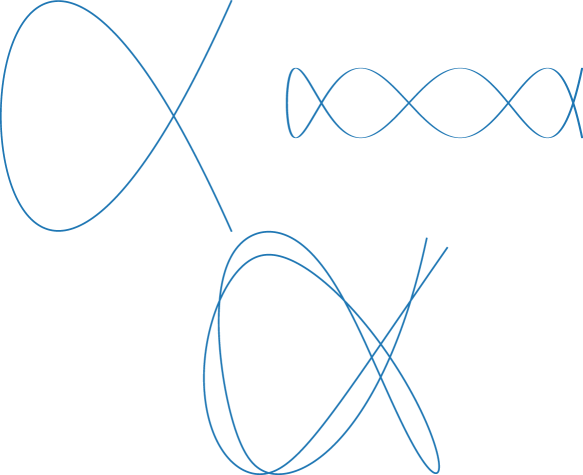
In general, for an isolated singularity of a real polynomial having several local branches, the divide of a real morsification may have immersed circles as components. The above cabling construction does not work if the divide consists of an immersed circle. Of course, if one is willing to change the equation of the singularity to an equation, which defines a topologically equivalent singularity and which has only real local branches, one will only have to deal with divides consisting of immersed intervals. If we do not want to change the real equation, we conjecture how a different type of block would produce real morsifications for these real singularities. Note that the question whether any real singularity admits a morsification or not is still open. See [LS18] for some partial results to answer the question in the positive and see [FPST22] for other recent conjectures that relie on this open question.
We conjecture that, if the real plane curve contains pairs of complex conjugate branches, then we could still produce divides using a second type of building blocks for a cabling construction, see Fig. 5.3.5.
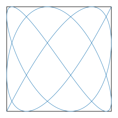
These building blocks are the divides in the annular region . If for the integers holds, the divide is the Lissajous curve
in . The curve has -fold rotational symmetry. If the divide is defined defined as the union of rotated copies of with rotations of angles of . Again, the system of curves has a -fold rotational symmetry.
The star-product can be defined as above if the divide consists of one immersed circle. The two types of building blocks and together with the star-products and will allow one to describe the iterated cablings of real plane curve singularities in general.
Natural orientations
The link of a divide is naturally oriented by the following recipe. Let be a local regular parametrization of . The orientation of is such that the map is oriented. Here is a positive scalar function, which ensures that the map takes its values in . For a connected divide we orient its fiber surface such that the oriented boundary of coincides with the orientation of .
Vanishing cycles where is a critical point of do not carry a natural orientation, since, for example, the third power of the geometric monodromy of the singularity reverses the orientations on the vanishing cycles.
We orient the tangent space so that the orientation of its unit sphere as the boundary of its unit ball gives that the linking numbers of and are positive for generic pairs of divides and . In fact, the orientation is opposite to its orientation as tangent space. With this convention, we have , a fact which was already used in the previous section.
6. Description of the Milnor fiber
In this section, we give a description of the Milnor fibers associated to a divide that lie over the points and . The description is done in terms of more simple pieces. This decomposition is useful in the forthcoming sections where we describe the geometric monodromy associated with the divide.
6.1. Description of the Milnor fibers over and
Let be a connected divide and let be its fibration of Theorem 4.1.1. In this subsection, we show how to read off geometrically the fibers and . For our construction we assume the disk oriented. We think of its orientation as an orthogonal complex structure . Define
The level curves of define a oriented foliation on , where a tangent vector to a level of at is oriented so that Put
and
where is the foliation with the opposite orientation. Put
for a maximum and
for a minimum of . For saddle points of (equivalently, double point of ), define
and
Observe that the angle in between or is a natural distance function on or which allows us to identify and with a circle. Finally, put
Let be the projection The projection maps each of the sets and homeomorphically to The sets or are homeomorphic to if or is a maximum or minimum of respectively. And the sets are homeomorphic to a disjoint union of two open intervals if is a crossing point of The set is homeomorphic to a disjoint union of open intervals. We have the following decomposition of :
Where denotes the set of double points of the divide. Observe that for we have (recall eq. 3.2.3) since and . So is an open and dense subset in . Accordingly, with the obvious changes of signs, we get a similar description for :
6.1.1. Combinatorial description
Forming the closure of in leads to the following combinatorial description of the above decomposition. First, we add to the open surface its boundary and get
Now let be a connected component of The inverse image in are two disjoint open cells or cylinders and which are in fact subsets of The closure of in is a surface with boundary and corners. The set is a common boundary component without corners of and if is a maximum in If there is no maximum in the closures and meet along the component of which lies in the closure of Let be connected components of such that the closures of and have a crossing point in common. The closures of and in meet along one of the components of and the closures of and in meet along the other component of The closure of in intersects in corners, that are also corners of the closure of in (see Fig. 6.1.1). Notice that the foliation on does not lift to a foliation, which extends to an oriented foliation on .

6.2. Description of the Milnor fibers over and
Now we quickly work out the fibers and Observe that and are projected to a subset of by . Put
For a crossing point of we put
Observe that
and recall (eq. 3.2.3). In order to get nice sets it is necessary to choose a nice bump function as before. The set
is an open and dense subset in and forming its closure results in
leads to a combinatorial description of similar to the one given above.
We would like to direct the interested reader to some beautiful pictures in the works of Sebastian Baader, Pierre Dehornoy and Livio Liechti [BD12, DL19] which complement the ones contained in this work and which exemplify how the Milnor fiber(s) are recovered from the divide. The referee called our attention to these works and we are thankful for that.
7. Descriptions of the monodromy
In this section we give a complete description of the geometric monodromy of the fibered link .
In Sect. 7.1 we give the monodromy as a composition of right-handed Dehn twists. This factorization, certainly completely determines the monodromy but it is general not trivial to give the Nielsen-Thurston decomposition from a factorization. In Sect. 7.2 we take care of this and give the minimal reduction system of curves of the Nielsen-Thurston decomposition of the monodromy.
7.1. Monodromy as a product of Dehn twists
We will use the integral curves of the distribution which pass through the crossing points of the divide In a connected component of , those integral curves of meet at the critical point of in the component with distinct tangents, or they go to distinct points of
We denote by the union of the integral curves of which pass through the crossing points of The complement in of the union is a disjoint union of tiles, which are homeomorphic to open squares or triangles
Notation 7.1.1.
We call a pair of tiles opposite, if and the closures of and in have a segment of in common. For an opposite pair of tiles let be the interior in of the union of the closures of and in .
The set is foliated by the levels of and also by the integral lines of the distribution Both foliations are non-singular and meet in a -orthogonal way (see Fig. 7.1.1).
Notation 7.1.2.
For a pair of opposite we put,
and
The sets and each have two connected components:
where
and
The closures of in and of in are polygons with edges: let be the vertices of the triangle ; the six edges of the closure of in are
where and are segments included in and is a segment in Next, we define two diffeomorphisms
and
for each pair of opposite tiles . To do so we choose the adapted function (recall Definition 3.2.1 and Lemma 3.2.2) such that the maxima are of value and the minima of value Moreover, we modify the function at the boundary such that along each of the integral lines of the foliation given by the distribution the function takes all values in an interval with . The latter modification of is useful if the tile or meets . We also need the rotations about the angle Recall that the complex structure is precisely .
We are now ready to define the map . Let with and do as follows:
-
(1)
let be the point in the opposite tile on the integral line of the distribution with
-
(2)
now move to along the integral curve which connects and with the parameterization ;
-
(3)
consider the rotation angle function and move the vector along the path
where is the continuous vector field along such that , we have the equality , and the stretching factor is chosen such that holds.
-
(4)
We finally define
The definition of is analogous, but uses rotations in the sense of .
The names or indicate that the flow lines pass through the fiber or respectively. The flow lines defining or are different. However, the maps and are equal. The system of paths is local near the link , i.e. for every neighborhood in of a point there exists a neighborhood of in such that each path with stays in . It will follow that the flow lines of the monodromy vector field are meridians of the link in its neighborhood.
Remark 7.1.3.
After verifying that the constructed flow lines form a monodromy flow for the , this last fact proves that the map is a fibration near the link . Proving this was a step in the proof of Theorem 4.1.1 and this is an alternative proof.
The partially defined diffeomorphisms and glue to diffeomorphisms
where the sum ranges over all opposite pairs of tiles with . The gluing poses no problem since those unions are disjoint, but the diffeomorphisms and do not extend continuously to We will see that the discontinuities, which are the obstruction for extending and can be compensated by a composition of right half Dehn twists (recall Definition 2.1.3).

At a maximum of each vector belongs to Let and be the integral curves of with one endpoint at and orthogonal to We assume that neither nor passes through a crossing point of (see Fig. 7.1.2) and that and belong to different pairs of opposite tiles. A continuous extension of the maps or has to map the vector to two vectors based at the other endpoint of and Since these endpoints differ in general, a continuous extension is impossible.
In order to allow a continuous extension at the common endpoint of and we make a new surface by cutting along the cycles where runs through all the maxima of and by gluing back after a rotation of angle of each of the cycles In the analogous manner, we make the surface in doing the half twist along where runs through the minima of The subsets do not meet the support of the half twists, so they are canonically again subsets of which we denote by Analogously, we have subsets in A crucial observation is that the partially defined diffeomorphisms
have less discontinuities, which are the obstruction for a continuous extension. We denote by and the arcs on which correspond to the arcs and on Indeed, the continuous extension at the end points of and is now possible.
Let be a crossing point of and let be the segment of which passes through and lies in The inverse image of is not a cycle, except if both endpoints of lie on If a maximum of is an endpoint of the inverse image consists of points on which are antipodal. On the new surface the inverse image is a cycle. An extension of and will be discontinuous along this cycle (see Fig. 7.1.3). We now observe that the partially defined diffeomorphisms and have discontinuities along the cycle , which can be compensated by half twists along the inverse images where runs through the crossing points of Note that for a crossing point of the curve is in fact a simply closed curve on .

For a crossing point of the divide we now define a simply closed curve on by putting:
where for an endpoint of which is a maximum of the set is the simple arc of which connects the two points of and contains an inward tangent vector of at As we already have noticed the set has only one element if so we define in that case.
We have the inclusion We now define the cycle Define for a minimum of the region
Let be the level curve
For a small the set
is a union of copies of an open interval and is not a cycle but nearly a cycle. The union closes up to a cycle by adding small segments which project to the integral lines through the crossing points of We denote this cycle by .
We are now able to state the main theorem.
Theorem 7.1.4.
Let in be a connected divide. Let be the fibration of Theorem 4.1.1 The counter clockwise monodromy of the fibration is the composition of right handed Dehn twists
where is the product of the right handed twists along running through the minima of is the product of the right handed Dehn twists along the cycles running through the crossing points of and is the product of the right handed twists along running through the maxima of
Proof.
We need to introduce one more surface. Let be the surface obtained from the surface by cutting along the cycles and by gluing back after a half twist along each with running through the crossing points of . We still have partially defined diffeomorphisms
since the cutting was done in the complement of By a direct inspection we see that the diffeomorphisms extend continuously to
Let
be minimal positive pairs of Dehn twists (recall Definition 2.1.3). A direct inspection shows that the composition
is the monodromy of the fibration This composition evaluates to
∎
Some consequences
Next we state some inmediate consequences of the previous constructions.
Remark 7.1.5.
We list some special properties of the monodromy of links and knots of divides. The number of Dehn twists of the above decomposition of the monodromy equals the first betti number of the fiber, and the total number of intersection points among the core curves of the involved Dehn twists is less then This means that the complexity of the monodromy is bounded by a function of . For instance, the coefficients of the Alexander polynomial of the link of a divide are bounded by a quantity, which depends only on the degree of the Alexander polynomial. This observation suggests the following definition for the complexity of an element of the mapping class group of a surface: the minimum of the quantity over all decompositions as product of Dehn twists of where is the number of factors and is the number of mutual intersections of the core curves. We do not know properties of this exhaustion of the mapping class group. Notice, that the function defines a left invariant distance on the mapping class group.
Remark 7.1.6.
It can be seen (see next Sect. 7.2) that for any link of a divide the monodromy diffeomorphism and its inverse are conjugate by an orientation reversing element in the mapping class group. In our previous notations this conjugation is given by the map
which moreover realizes geometrically the symmetry of G. Torres [Tor53]
for the Alexander polynomial of knots.
Remark 7.1.7.
In fact the proof of Theorem 7.1.4 shows that the fibration of the link of a connected divide can be filled with a singular fibration in the -ball, which has singular fibers with only quadratic singularities, as in the case of a divide of the singularity of a complex plane curve. The filling has only two singular fibers if the function has no maxima or no minima. By this construction from a connected divide we obtain a contractible -dimensional piece with a Lefschetz pencil. This is part of what is usually called Hurwitz equivalence. For more on this topic, see the classical references by Kas [Kas80] or Matsumoto [Mat96], or the more recent by Baykur and Hayano [BH16].
We make the following important observation that we have not lost generality by considering only divides which are generic immersions of intervals.
Remark 7.1.8.
It is important to note that Theorems 4.1.1 and 7.1.4 remain true for generic immersions of disjoint unions of intervals and circles in the -disk. It is also possible to start with a generic immersion of a 1-manifold in an oriented compact connected surface with boundary The pair defines a link in the -manifold
where is the space of oriented tangent directions of the surface and where zip is the identification relation, which identifies if and only if or if In order to get a fibered link, the topological pair has to be contractible for each connected component of and moreover, the complement has to allow a chess board coloring in positive and negative regions. For more details on this construction, see [Ish04].
7.2. Other decompositions of monodromy
In this subsection we study yet a decomposition of the algebraic monodromy in terms of involutions. The contents of this section come mainly from [A’C03].
Digression in higher dimensions
We start with a discussion about geometric monodromies of isolated hypersurface singularities in general dimension (recall the discussion of the subsection 2.2 on page 2.2).
Let be a map defined by a polynomial. We assume that and that is an isolated critical point of . For let
Let be a Milnor ball for the singularity of and let
be a regular tubular neighborhood of in . A monodromy vector field for the singularity is a smooth vector field
such that we have the following properties for
-
•
,
-
•
is tangent to if ,
-
•
trajectories of starting at are periodic with period and are the boundary of a smooth disk in , that is transversal to the function . For this property to be satisfied, the hypothesis that has a critical point is crucial.
Using partition of unity, one can construct monodromy vector fields. The flow at time of a monodromy vector field defines a monodromy diffeomorphism , where the manifold with boundary is the Milnor fiber of the singularity. The relative isotopy class of the diffeomorphism is independent from the chosen monodromy vector field and is called the geometric monodromy of the singularity. The geometric monodromy is a topological invariant of the singularity (see [Kin78, Theorem 3] for and [Per85] for ).
From now on we will assume in addition, that the polynomial is real meaning that its coefficients are real numbers. Let denote the involution on complex space given by the complex conjugation of coordinate values. Hence with the above notations, we have and . We denote by the restriction of the involution to .
Let be a monodromy vector field for the isolated singularity of . We may assume that we have constructed the vector field with more care near the boundary of the Milnor ball in order to achieve that for some we have the symmetry
Since is real, we have
hence, we see (by substituting for and accordingly for ) that the vector field defined by:
is a monodromy vector field too. Let be the vector field
which due to the extra care is also a monodromy vector field. We have . The following is an important symmetry of the geometric monodromy:
Lemma 7.2.1.
Let be a monodromy diffeomorphism, which has been computed with a monodromy vector field satisfiyng . We have the symmetry
The geometric monodromy satisfies (up to relative isotopy) the symmetry
Proof.
The restriction of complex conjugation maps the monodromy vector field to and to . Hence, since reverses the orientations of the trajectories, we have
Since the geometric monodromy is in the relative mapping class represented by , we have the symmetry at the mapping class group level. ∎
Symmetries of monodromies as in the lemma can occur in the more general context of so-called strongly invertible knots, see for instance [Tei90, HT78, Kaw96].
See also the work of Sabir Gusein-Zade [GZ84], in which he shows among other results, that the integral homological monodromy of an isolated complex hypersurface singularity with real defining equation is the composition of two involutions, both conjugated to the action of complex conjugation on the homology of a real regular fiber.
Remark 7.2.2.
The symmetry property expresses that the geometric monodromy of a complex hypersurface with real defining equation is conjugate in the mapping class group by an element of order to its inverse . This is a statement in the mapping class group of the Milnor fiber and does not refer to any complex conjugation, so it can be stated for any complex hypersurface singularity with complex defining equation. We say that the singularity is strongly invertible if its geometric monodromy diffeomorphism is conjugate by an element of order in the relative mapping class group of the Milnor fiber to its inverse . Thus, the property of strong invertibility is a topological property for hypersurface singularities.
We can rewrite the symmetry property as follows: . We see that is an involution of . It follows the
Corollary 7.2.3.
The geometric monodromy of an isolated complex hypersurface singularity, which is defined by a real equation, is the composition of two involutions of the fiber namely: , where is the restriction of the complex conjugation.
For we also have the relation , which shows that is a sequence of involutions of .
The above observations can be applied to plane curve singularities in general, since it follows from the Theory of Puiseux Pairs that every plane curve singularity is topologically equivalent to a singularity given by a real equation and hence plane curve singularities are strongly invertible.
For complex hypersurface singularities of higher dimension the situation seems to be opposite. In there exist isolated hypersurface singularities which are not topologically equivalent to a singularity with a real defining equation [Tei90]. We expect that in general the geometric monodromy of a complex hypersurface singularity fails to be strongly invertible.
Mathias Schulze communicated to the first author a proof of strong invertibility of the homological monodromy with real coefficients (this was never published and stayed as a personal communication). The following is a strengthening of his result to the case of homology with rational coefficients.
Theorem 7.2.4.
The rational homological monodromy of a complex hypersurface singularity is strongly invertible.
Proof.
Let be a finest possible direct sum decomposition in -invariant -subspaces of . The characteristic polynomial of the restriction of to a summand is a power of a cyclotomic polynomial . We have by the Hamilton-Cayley theorem and we have since a power of cyclotomic polynomial satisfies .
Since the decomposition has no refinement, we may choose a vector , that is cyclic for and for . The systems
are basis for the space . Let be the linear map defined by .
We have . The polynomial satisfies . Since the degree of the polynomial is less than , we have
We conclude that and hold.
The polynomial satisfies and . We deduce and conclude . We observe at this point that both the conjugates of by and by are equal to the inverse .
For we have (remember )
Hence is of order two, which shows that is strongly invertible over . The direct sum is a rational strong inversion for . ∎
Question: Is the integral homological monodromy of a complex hypersurface singularity strongly invertible? For example, take the isolated surface singularity
where are linear forms on , such that the lines in the complex projective plane span the configuration of flex tangents to a nonsingular cubic. No real equation for this singularity can exist, since the configuration cannot be realized in the real projective plane, see [Tei90, HCV32]. Is its monodromy strongly invertible?
Going back to plane curves and divides
Now we focus on the study of complex conjugation on the topology of plane curve singularities via divides. First we show that the fiber of the link of a connected divide carries naturally a cellular decomposition with tri-valent -skeleton.
Let define an isolated plane curve singularity at given by a real convergent power series . Let be the factorization in local branches. The topology of a plane curve singularity is completely encoded in a divide for as we have seen in Sect. 4 or in the previous section where we have given a factorization of the monodromy from the divide. (c.f. [A’C99, BK96]), see also [A’C75b, A’C75c, GZ74b].
We state the results more generally for links of connected divides, since the involution given by complex conjugation on real isolated plane curve singularities corresponds to a natural involution of links of divides as explained below, (c.f. [A’C98a, A’C99]).
Denote by the number of double points of the divide . The local topology of a plane curve singularity is obtained from a divide for the singularity. More precisely, the link of an isolated plane curve singularity is equivalent to the link of a divide , see Sect. 5 (c.f. [A’C99]).
We recall, that for a totally real (Definition 5.1.1) plane curve singularity one can obtain a divide by performing a small real deformation of the singularity, where for the restriction of to the euclidean disk of radius in is a Morse function with critical points and such that the -level is connected and contains all the saddle points (this is the content of Theorem 5.2.1). The divide for is the curve , which we rescale by the factor from into the unit disk .
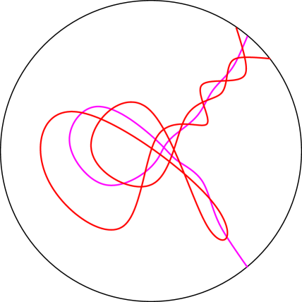
The homology can be described combinatorially in terms of the divide as a direct sum , where and are the subspaces in , which are freely generated as follows:
where is the oriented system of vanishing cycles of the divide with positive upper triangular Seifert form
see. We define , which is upper-triangular nilpotent matrix. The monodromy is given by:
For the rest of this section, recall the construction of the fiber surface of a divide in the unit euclidian disk . In particular, recall the notation from Sect. 3 and Sect. 5.
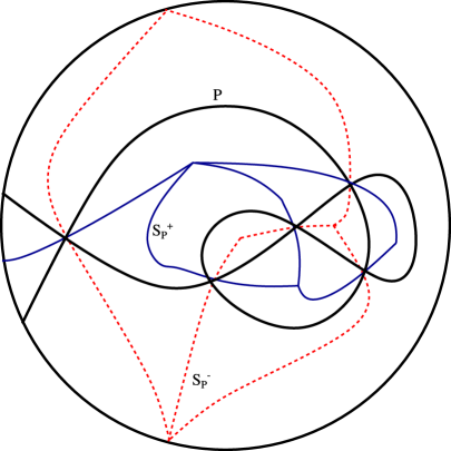
Let be a system of gradient lines of , which connect saddle points of with local or relative maxima or minima of . In fact, near the boundary of the lines of the system are only gradient-like, but end in a relative critical point of . We call the set the graph of the divide . By a slalom construction, see [A’C98b] (not included in this work), one can reconstruct from each of the sets the divide . We assume that at the maxima and minima of , that different arcs of have different unoriented tangent directions. Let be the following subset of the fiber over of the natural fibration over of the complement of the link of : the subset is the closure in the tangent space of of
We recall that the union of fiber with the link is the closure in of
which is a surface of genus equal to the number of double points in .
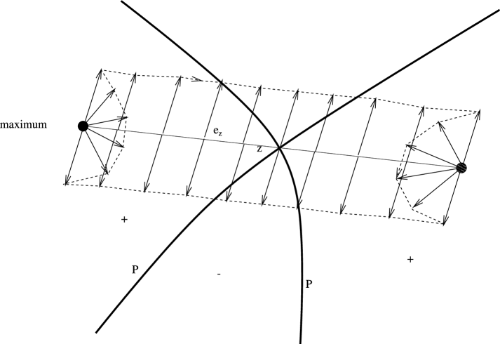
The system of cycles can be drawn on as follows. The vanishing cycle which corresponds to a local maximum of is the circle oriented counter clock-wise. The vanishing cycle which corresponds to a saddle point of is a curve in the set
as drawn in Fig. 7.2.3. The curve is a piecewise smooth embedded copy of in with image in and with non-constant projection to the disk . The orientation is chosen such that at both ends the orientation agrees with the oriented vanishing cycle of the maximum. Moreover, the inward tangent vectors to at end points do belong to . The vanishing cycle which corresponds to a local minimum of projects to an oriented circuit of edges of the graph . The circuit surrounds the region in counter clock-sense to which the minimum corresponds. The circuit is a polygon and bounds a cell in . The curve is a subset of and is the image of a piecewise smooth embedding of as drawn in Fig. 7.2.4. The vectors , which belong to , point out of the cell of the circuit. Smooth representatives for the system of vanishing cycles can be obtained using tears as in [A’C01] (see also Sect. 8.1).
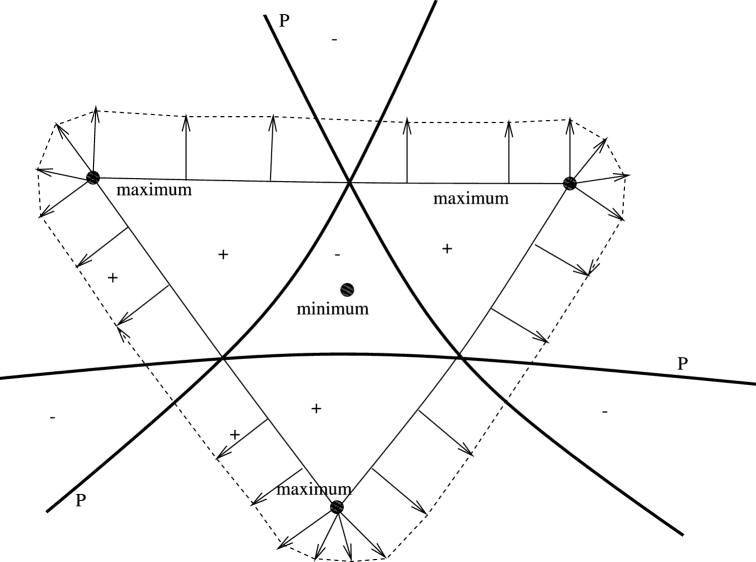
The involution induces an involution on that preserves the link of any divide and that induces involutions on the fiber surfaces above . If the divide is a divide for a real plane curve singularity , the involutions induced by or by the complex conjugation on the triples and on correspond to each other by the homeomorphism of pairs of the main theorem of (c.f. [A’C99]).
Theorem 7.2.5.
Let be a connected divide consisting of the image of a relative generic immersion of a compact one dimensional manifold in the unit disk . Let and be the summands in as above. The involution fixes point-wise the summand , in particular for we have
For we have
For we have
The trace of the involution is given by:
Proof.
A vanishing cycle corresponds to a maximum of , hence as set we have . The involution induces on the antipodal map, which is orientation preserving. It follows in homology. A vanishing cycle corresponds to a saddle point of . Working with the tear model of (c.f. [A’C01]), see also (the independent) Sect. 8.1, we see that the involution reverses the orientation and that at the endpoints, which are maxima of , we have outward instead of inward vectors. Hence,
where in the sum runs through the maxima of in the interior of which are connected by gradient lines of to the saddle point . The coefficient equals or depending on whether the connection by gradient lines is simple or double. Finally one gets . For a vanishing cycle one can work with the model of (c.f. [A’C01]) and get . Since is strictly upper-triangular, the matrix of is upper-triangular with on the diagonal. We get . ∎
We can present the Seifert form and homological monodromy with block-matrices as in [GZ84]. On and we work with the basis or dual basis given by the system . The matrix in block form of the Seifert form is
where the block equals the block matrix product . The matrix coefficients of and have interpretations in terms of the divide or in terms of the Morse function on the disk . The matrix coefficient counts the number of sector adjacencies, that has the -region of with the -region , while the coefficient counts the number of common boundary segments of the regions and . The coefficient also counts the number of saddle connections via gradient lines of in between the minimum and maximum , while the coefficient counts the number of components of regular gradient line connections from the minimum to the maximum . This explains the above factor , since a segment of is twice incident with a saddle point of .
The matrix of the action of complex conjugation on is
and is obtained from the matrix by multiplying the middle row of blocks by . It is interesting to compute the matrix of the involution on
The matrix is the transgradient of the matrix of .
It turns out that the combinatorial property for divides is equivalent to or .
For an isolated plane curve singularity at , which is given by a real equation we will denote by the number of double points of a divide for the singularity. Hence is the maximal number of local real saddle points in some level, that can occur for a small real deformation of . Observe, that one has , where is the maximal number of local critical points in some level, that can occur for a small deformation of . We recall the formula of Milnor [Mil68]. As example for one has and very surprisingly, Callahan shows that for there exists a small real deformation with local minima in the same level [Cal78].
Theorem 7.2.6.
For an isolated plane curve singularity at , which is given by a real equation we have
Proof.
We have Hence ∎
Curves that correspond to maxima of are invariant by the involution . A curve that corresponds to a saddle point or minimum of is in general not invariant by . The union of the curves is invariant by . We get
Theorem 7.2.7.
Let be a connected divide. The pair defines a tri-valent cellular decomposition with punctured cells of the fiber surface with boundary . The involution acts on the map .
Proof.
The union of the vanishing cycles is a tri-valent graph that is invariant by . The inclusion induces an isomorphism , hence, is a spine for the surface . ∎
Question. In particular if the triple is a so-called maximal unicell map of genus with orientation reversing involution with fixed points on the graph of the map. The involution has a unique fixed point on , which corresponds to the intersection of the folding curve of with the graph . Maximal here means that the number of edges of the graph of the map is maximal, i.e. .
It would be interesting to compute the generating series
where denotes the number of simple, relative and generic immersions of the interval with double points in the disk , counted up to homeomorphism in the source and image. We have taken the coefficients up to the term of from the listings of simple, relative, free or oriented divides by Masaharu Ishikawa [Ish01]. We ask to compare the numbers with the numbers of maximal maps of genus with orientation reversing involution having fixed point on its graph.
Involutions induced by -rotations
Next we study the involutions that appear in the decomposition of the geometric monodromy of plane curve singularities. We show that they lift to -rotations about an axis in the universal cyclic covering of the complement of the link.
Our next goal is to visualize the two involutions and . We assume that the monodromy diffeomorphism is chosen in its isotopy class such that is an involution of the fiber surface . In fact, we assume that the monodromy was given by a monodromy vector field , which satisfies .
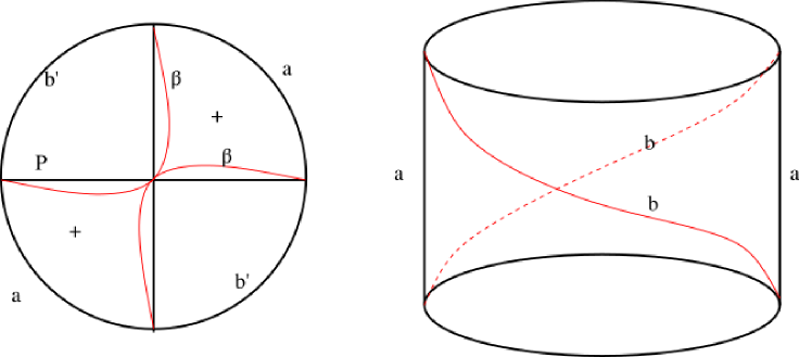
We assume for simplicity, that the divide meets the boundary of the disk . The involution is an orientation reversing diffeomorphism of , which fixes point-wise the system of arcs . The Lefschetz number of the orientation reversing involution is equal to the Lefschetz number of by Th. . Hence the involution also fixes point-wise exactly a system of arcs on the fiber surface with , i.e. the systems and consist of the same number of arcs.
Let be the infinite cyclic covering of the knot complement. Let be the lift of the vector field . Let be the flow diffeomorphism of the vector field with stopping time . Let be a lift of the fiber surface and let be the lift of the fiber surface . The involution can first be lifted unambiguously to an involution of and then extended unambiguously to an involution of such that maps the vector field to its opposite. The involution is a -rotation about a lift of the system of arcs into . The involution induces an involution of the fiber surface above , and, as we have done for the involution , the involution lifts unambiguously to a -rotation about a system of arcs that satisfies . We have . Since is a lift of the monodromy, it follows from , that the involution fixes the system of arcs .
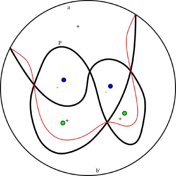
In Sect. 7.1 (c.f. [A’C98a]) we have computed the monodromy diffeomorphism for which is a lift to as a product of half Dehn twists for a divide. From the above we deduce, that the involution is the composition . We see that fixes the arc . We also see that the involution of fixes the system of arcs . Both arc systems and have equal projections into . See Figures 7.2.5 and 7.2.6 for examples.
The composition of the orientation reversing involutions, that fix point-wise the arc systems of Fig. 7.2.5 on the cylinder surface, is indeed a Dehn twist. To see this, think of the cylinder as ; the two involutions induce on the circle reflections about diameters that make an angle , so the composition is a rotation of angle of the circle .
In Fig. 7.2.6 the curve is drawn for a more complicated divide for the plane curve singularity with equation .
We conclude with a remark we promised that shows that uses the results of this section to prove that not all fibered links come from divides.
Remark 7.2.8.
The figure eight knot (see Fig. 3.1.2) is not the knot of a divide. The figure eight knot’s complement fibers over the circle having as fiber the punctured torus and as monodromy the isotopy class of the linear diffeomorphism given by a matrix in of trace . Such a matrix is not the product of two unipotent matrices, which are conjugate in and the matrices and are not conjugated by an integral matrix of determinant . So according to the remarks this section, the figure eight can not be the knot of a divide. Another argument to rule out the figure eight as the knot of a divide goes as follows. The first betti number of the fiber of the figure eight knot is . But only two connected divides have fibers with betti number and these two have monodromies with trace equal to or .
8. Abstract visualization of the Milnor fiber and the monodromy
In this section we describe an easy and fast graphical algorithm of visualizing the Milnor fiber together with a distinguished basis of vanishing cycles directly from the divide ([A’C99]).
8.1. Visualization of the vanishing cycles for a divide
We start by visualizing the vanishing cycles.
Let be a connected divide and let be the fibration of the complement of the link over as in Sect. 4 (c.f. [A’C99, A’C98a]). Recall that the fibration map is given with the help of an auxiliary Morse function . The fiber above projects to the positive components of the complement of in . One has that the closure of
in is the fiber surface .
To each critical point of corresponds a vanishing cycle on the surface . In the case, where the divide is a divide of a singularity, the surface is a model for the Milnor fiber and the system of vanishing cycles on is a model for a distinguished system of quadratic vanishing cycles of the singularity.
Let be a maximum of . The vanishing cycle is the non-oriented simply closed curve on , see Fig. 8.1.1,

Let be a crossing point of . The point is a saddle type singularity of . The vanishing cycle is the non-oriented simply closed curve on that results from the following construction. Let be the singular gradient line through , for which the endpoints are a maximum of or a point in . We splice and get a double tear as in Fig. 8.1.2. The tear is a closed curve, that has at a non-degenerate tangency with from both sides. Moreover, is perpendicular to at the endpoints of , if the endpoint is a maximum of and else has a tangency with . The vanishing cycle is the closure in of the set

Let be a minimum of . The following is a description of the vanishing cycle on . The projection of in is a simply closed curve in , where is the list of the double points of that lie in the closure of the region of , see Fig. 8.1.3. The curve and the singular gradient line coincide in a neighborhood of . Moreover, if the endpoint of is a maximum , the curve leaves transversally the tear at and enters transversally the next tear . If the endpoint of is on the boundary of , the curve leaves the tear , becomes tangent to the boundary of and enters the next tear, see Fig. 8.1.3. The vanishing cycle is the non-oriented simply closed curve on , that is the closure of

8.2. Visualization of the Milnor fiber associated with a divide
Now we explain how to visualize the Milnor fiber together with the divide. Think of the divide as a road network which has junctions, and replace every junction by a roundabout, which leads you to a new road network with T-junctions. Realize now every road section in between two T-junctions by a strip with a half twist. Do the same for every road section in between a T-junction and the boundary of the divide. Altogether you will need strips. Now, applying what we have seen in the previous Sect. 8.1, the core line of the four strips of a roundabout is a black vanishing cycle, the strips corresponding to boundary edges and corners of a positive or negative region have as core line a red or blue vanishing cycle (see Fig. 8.2.1 or 8.2.2 for color scheme).
In Fig. 8.2.2 is worked out the singularity with two Puiseux pairs and , where we used a divide equivalent (up to an admissible isotopy) to that of Fig. 5.3.3. We have drawn for convenience in Fig. 8.2.2 only one red, black, or blue cycle. We have also indicated the position of the arc which will play a role in the next section.
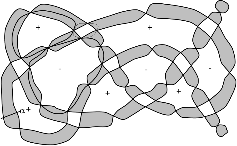
8.3. Reduction cycles and reduction tori
We consider a divide of the form , where the divide is given by an immersion . So, the divide is the image of . If we change the immersion by a reparametrization , where is an oriented diffeomorphism of , the divide is isotopic to by an transversal isotopy, which does not change the type of its knot. By choosing appropriately and small, one can achieve that to each double point of correspond double points of the divide , which look like the intersection points of a system of almost parallel lines with an other system of almost parallel lines, see Fig. 8.3.1.
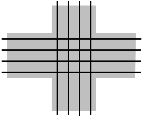
We may assume, that the divide for each double point of already has a grid of intersections.
We will construct reduction curves for the monodromy of the knot following the ideas of [A’C73]. The reduction curves of the cabling are the intersection of the fiber over of the fibration on the complement of the knot with the boundary of a regular tubular neighborhood of the closed tubular neighborhood of the knot for which holds. The intersection is indeed a system of reduction curves provided that the torus is transversal to the fibration of the knot .
Assume that the tubular neighborhood was constructed with the field and a particular value of the parameter . The same field of sectors, but a slightly bigger parameter value yields a tubular neighborhood of in . The construction of the fibration will be done as in Sect. 4 (c.f. [A’C98a]). The main choice for the construction of the fibration for the knot is a carefuly chosen adapted Morse function (recall Definition 3.2.1) with . For our purpose here, where we must achieve the above transversality so we will choose as follows. First, after applying a regular transversal small isotopy, we may assume that the divide has perpendicular rectilinear crossings. Next, we consider an adapted function for the divide , that is euclidian near its crossings. Let the fibration on the complement of the knot be where we recall that and
Here, the function is a bump function at the crossing points of and is a big real parameter (compare with eq. 3.2.3). We now choose a small positive real number , such that is a regular tubular neighborhood of , that meets each component of . Next we choose such the corners of are in i.e. . We constuct the torus knot with where . Since holds, we can construct a Morse function for the divide , such that on the function is constant along the level sets of .
The following theorem follows directly from [A’C73, Lemme , pg. ] and the above construction.
Theorem 8.3.1.
The torus is transversal to the fibration induced by on the complement of the knot . The intersection
is a system of closed curves on the fiber , which is a reduction of the monodromy of .
With a few examples, we now explain how to inductively depict in the Milnor fiber a distinguished system of vanishing cycles and the reduction curves for the monodromy of a singularity, for which a divide of the form is given.
For a cabling () the reduction system consists of simply closed curves on the fiber . Each of them cuts out from a surface diffeomorphic to the fiber of the divide . The copies of in are cyclicly permuted by the monodromy . This description follows from the construction of the monodromy of an irreducible plane curve singularity given in [A’C73].
One of those copies can be visualized more easily as follows. Let . For each double point of we connect the two components of , that are incident with the double point , by a special bridge which projects diagonally through the Manhattan part of the divide , that corresponds to . The projection of the bridge is a twisted strip in , that realizes a boundary connected sum of the -components (see Fig. 8.3.2). The twist points of the strip are precisely the critical points of , that lie on the diagonal. The boundary of consists of two smooth curves, that intersect each other transversally and that also intersect the divide transversally.
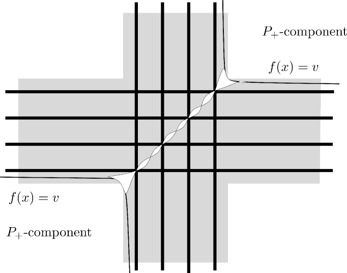
Let be the union of the projections of the bridges with , see Fig. 8.3.2. In Fig. 8.3.3 we have zoomed out one block to show more details. The copy of the fiber of the knot is the closure in the fiber of the knot of the set
The first reduction curve is the boundary
of the surface . The reduction system is the orbit
under the monodromy of the singularity with divide .
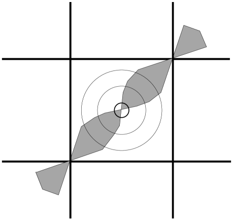
Example 8.3.2.
Our first example is the singularity with two essential Puiseux pairs , whose link is a two stage iterated torus knot. For a detailed description of the link, the monodromy and the Milnor fiber of this singularity, follow the construction of [A’C73]. Its divide , (see Fig. 5.3.3), has two -components, where (recall Fig. 8.3.4 and contents of that section), where the projection of the reduction curve is drawn). In this case Manhattan consists of one block. The reduction curve is the pre-image in the fiber of its projection under the map (see Fig. 8.3.4). That means is the closure in of the set
The reduction system is .

The curve is homologically trivial in . It turns out that the power of the monodromy is the composition of the right Dehn twists, whose core curves are . The power is a product of Dehn twists, since is the product of those Dehn twists whose core curves are the system of distinguished quadratic vanishing cycles of the real morsification with divide . It turns out that the expression as product of Dehn twists is far from being as short as possible. In fact, the right Dehn twist with core curve can be written as a product of right Dehn twists that have core curves coming from the morsification with divide . More precisely, the Dehn twist factors as
The factors are right Dehn twists whose core curves are among the quadratic vanishing cycles of the divide as indicated in Fig. 8.3.3, is the vanishing cycle of a -region, of the maximum of Manhattan, and of street corners of Manhattan. It follows that can also be written as a composition of Dehn twists with core curves among the vanishing cycles of the divide . The composition is the Dehn twist with core curve .
The reduction curve cuts off from a piece of genus one, which corresponds to a copy of the Milnor fiber of the Brieskorn-Pham singularity (corresponding to the first Puiseux pair). The Dehn twists and act only on this piece, since the curves and lie entirely in this piece; in this piece, that is a copy of the fiber , they generate the geometric monodromy group of the accompanying singularity with divide .
Example 8.3.3.
Our second example is the double cusp, that is, the singularity with two branches . Its homological monodromy is of infinite order by [A’C73]. Each branch is a torus knot. Again Manhattan consists of one block. In Fig. 8.3.5 we have drawn the projections of the curves and , that together are the boundary components of the two diagonals through Manhattan. In this case the curves and are isotopic to each other, as are the curves and . A complete reduction system for the geometric monodromy is the system . Each component of this system carries a non-trivial homology class. The isotopy classes of the curves and are permuted by the monodromy , hence the system is invariant under the monodromy.

Let be the action of on the homology of the the fiber . Let be the vanishing cycles of the double points, that are the corners of Manhattan of , let be the vanishing cycle of the maximum in the center of Manhattan.
If one chooses the orientations appropriately, on has
hence also . Let be any cycle on , that is carried by a simple oriented curve and intersects the curves and each transversally in one point. One has , which shows that the homological monodromy is not of finite order. We have drawn in Fig. 8.3.5 the oriented projection of such a cycle , that intersects the curves and . The curve is halfway in between the curves and on the cylinder they cut out. Let be the curve halfway in between and . The curves and are the reduction curves of Figure on page of [A’C73]. The reduction system is much easier to draw, see Fig. 8.3.6, where are drawn the projections in . The projections meet transversally at the maximum in Manhattan of . The curve intersects transversally in two points each curve and . One has .

The power of the geometric monodromy, that is a word of length in the Dehn twists of the divide , is equal to the composition of those right Dehn twists, whose core curves are and . So, the power also can be written as the much shorter word
Remark 8.3.4.
The curves and are isotopic, where and are the right Dehn twists with core curves and . It follows that the reduction system consists of quadratic vanishing cycles of the singularity of with two branches. In contrast, a reduction curve of a singularity with only one branch can not be a quadratic vanishing cycle, since all reduction curves are zero in the homology.
8.4. Geometric monodromy group and reduction system
Let the polynomial be an equation for an irreducible plane curve singularity with essential Puiseux pairs with . The number of simply closed curves contained in a complete reduction system for the monodromy of is
Indeed, this follows from the construction of the Milnor fiber in [A’C73]. Let
be the subgroup of the geometric monodromy group (recall Definition 2.3.2) of of of those elements that up to isotopy fix each component of . Let be the subgroup of which is generated by the Dehn twist whose core curves are quadratic vanishing cycles and do not intersect any component of . Obviously, one has , but we do not know if this inclusion is strict. A component of is called a top-component if its closure in meets only one component of . Let be the subgroup of of those monodromy transformations, which induce the identity in each component of that is not a top-component. Let be the intersection . We have
Theorem 8.4.1.
Let be an irreducible singularity with essential Puiseux pairs . Let be a singularity with the essential Puiseux pairs . The group contains the product of copies of the group .
Theorem 8.4.2.
Let be an irreducible singularity with essential Puiseux pairs. The group is isomorphic to the product of copies of the geometric monodromy group of the singularity .
Proof of Theorem 8.4.1.
Let be the divide for the singularity of and let be the divide for the singularity of . A copy of the fiber is constructed as a subset of the fiber . Remember, that is obtained by connecting with strips the sets , where is a Morse function for the divide . For each double point of there are two connecting strips. To each -component of corresponds a -component of with the same topology and to each double point of corresponds a Manhattan grid of , in which we have drawn diagonally the projection of the strips that connect . Here, denotes the union of the -components of the complement of the divide . From the divide is deduced a distinguished basis of quadratic vanishing cycles for the singularity of . Let be the union of the curves of this basis. This basis can be drawn on the fiber , see Sect. 8.1 for an algorithmic method to visualize distinguished basis of vanishing cycles.
In order to prove the theorem, we will construct inside a system of simply closed curves with union , each of them being a quadratic vanishing cycle for the singularity , such that the pairs and are diffeomorphic. This finishes the proof, since the Dehn twist, whose cores are the quadratic vanishing cycles of , generate a copy of in . By acting with the geometric monodromy of the singularity , one obtains commuting copies of in .
To each -region of corresponds one -region of . The maximum of , say at in the region, is also a maximum of . The quadratic vanishing cycle of lies in and also in . For each double point of the quadratic vanishing cycle projects in to a tear splicing the gradient line of through . The endpoints of are maxima of or points on . The function has exactly one gradient line that has the same endpoints as and coincides with in a neighborhood of the common endpoints. The gradient line runs along a diagonal through the Manhattan grid corresponding to . Let be the simply closed curve on , that projects to a tear equal to , except above a neighborhood of its endpoints where equals . We remark that is a cycle in . Let be the double points of that occur along the and let along be the maxima. Let be the quadratic vanishing cycle of the singularity that corresponds to . One verifies that the cycles and
are isotopic. Here or stands for the right Dehn twist of whose core curve is the quadratic vanishing cycle or of the singularity . Hence is a quadratic vanishing cycle for the singularity . So far, we have constructed for each maximum and for each saddle point of a simply closed curve on that is a quadratic vanishing cycle of the singularity . These cycles intersect on as do the corresponding quadratic vanishing cycles of the singularity on .

We now wish to construct for each minimum of a vanishing cycle on . We have to handle two cases: odd, see Fig. 8.4.1, and even, see Fig. 8.4.2.
If is odd, a minimum of will also be a minimum of . Let be the vanishing cycle on corresponding to , see Fig. 8.4.1. The projection of into is a smooth simply closed curve transversal to , that surrounds the region of through the its neighboring regions of . One needs to take care that in each neighboring component the projection runs through the maximum of in that region. The points of correspond to pairs with and pointing inwards to . Let be a simply closed cycle on that projects into upon the curve , which now surrounds the region of through the -components of , see Fig. 8.4.1. In the Manhattan grids ist just a diagonal, again runs through the maxima of the regions or touches . On we only allow pairs where points inwards to . It is clear that the cycle on intersects the cycles of the previous construction as the vanishing cycle to the minimum of intersects the vanishing cycles of the critical points of . It remains however to check that the cycle is a quadratic vanishing cycle of the singularity of . By applying to the Dehn twist corresponding to the critical points of that are in between the curves and , one can transform the isotopy class of the curve to the class of the curve . This proves that is indeed a quadratic vanishing cycle of the singularity of .

If is even, a minimum of will be a maximum of . Let be the vanishing cycle on corresponding to maximum , see Fig. 8.4.2. Its projection into is the point . Let be a simply closed cycle on that projects into upon the curve which now surrounds the region of through the -regions of , see Fig. 8.4.2. In the Manhattan grids ist just a diagonal, again runs through the maxima of the regions. On we only allow pairs where points inwards to . It is clear that the cycle on intersects the cycles of the previous construction as the vanishing cycle to the minimum of intersects the vanishing cycles of the critical points of . By applying to the Dehn twist corresponding to the critical points of that are in between the curve and the point , one can transform the isotopy class of the curve to the class of the curve , and proves that is indeed a quadratic vanishing cycle of the singularity of . As explained, this terminates the proof. ∎
Proof of Theorem 8.4.2.
The proof of Theorem 8.4.1 constructs a copy of the monodromy group of the singulatity as subgroup in the monodromy group of the singularity . This copy acts with support in a copy of the fiber . The the first iterates of the monodromy of the singularity constructs copies of in . By conjugation with one gets copies from . We end the proof by repeating this argument. One gets commuting copies of the geometric monodromy group of the singularity in . ∎
9. Some other questions and properties
We conclude by stating some other open questions and properties related to divides associated with plane curve singularities.
9.1. Connected sum and characterization of plane curve divides
The connected sum of two divides and is done by making a boundary connected sum of and such that a boundary point of matches with a boundary point of For divides with one branch we have the formula:
A relative immersion of a copy of in such that at selftangencies the velocities are with opposite orientation, defines an embedded and oriented arc in by putting:
Let be a relative immersion with only transversal crossings and opposite selftangencies, such that the endpoints of and are tangent with opposite orientations and that all tangencies of and are generic and have opposite orientations. The union is the oriented knot of the pair A divide defines pairs of relative immersions with opposite orientations by taking both orientations. Those pairs have a special -fold symmetry. For instance the complex conjugation realizes this -fold symmetry for a divide, which arises as a real deformation of a real plane curve singularity. It is interesting to observe that this symmetry acts on with as fixed point set the intersection , which is a collection of disjointly embedded arcs in The quotient of by the symmetry is an orbifold surface with exactly boundary -singularities. Any link of singularity of a plane curve can be obtained as the link of a divide by Sect. 5 (c.f. [A’C75b, A’C99, GZ74b]). It is an interesting problem to characterize links of singularities among links of divides.
9.2. Symplectic properties
The link of a divide is transversal to the standard contact structure in the -sphere. This can be seen explicitly by the following computation, where we use the multiplication of quaternions. Let be a divide in the unit disk. We assume that the part of , which lies in the collar of with inner radius , consists of radial line segments. We think of the branches of as parametrized curves where the parameter speed is adjusted such that To the branch correspond two arcs and on the sphere of quaternions of unit length:
The left invariant speed of at time is
We have
The coefficient vanishes, since is perpendicular to and hence we can rewrite the coefficient of in as
Outside of the collar neighborhood of we have since In the collar we also have by a direct computation. Since the left invariant contact structure on the unit sphere in the skew field of the quaternions is given by the span of the tangent vectors and at the point , we conclude that with its orientation is in the positive sense transversal to the left invariant contact structure .
For the link of a divide we now will construct a polynomial, hence symplectic, spanning surface in the -ball. For put
We have and is a strictly holomorphically convex domain with smooth boundary in . The map identifies with the unit -sphere of .
Theorem 9.2.1.
Let be a connected divide in the disc with double points and branches. There exist and there exists a polynomial function with the following properties:
-
(a)
the function is real, i.e.
-
(b)
the set is a divide, which is close to the divide P, and hence the divides and are combinatorially equivalent,
-
(c)
the function has only non degenerate singularities, which are all real,
-
(d)
for all the intersection is transversal and by a small isotopy equivalent to the link ,
-
(e)
for the link the surface is a connected smooth symplectic spanning surface of genus in the -ball.
Proof.
Let the divide be given by smooth parametrized curves . Using the Weierstrass Approximation Theorem, we can construct polynomial approximations being close to and henceforth give a divide with the combinatorics of the divide We may choose such that Let be a real polynomial map such is a regular equation for the union of the images of Let be the sphere For a sufficiently small we have that the -level of on is a model for the link For and sufficiently small, say , the surface is connected and smooth of genus , and has a polynomial equation, hence is a symplectic surface in the -ball equipped with the standard symplectic structure of The intersection is also a model for the link and has hence a symplectic filling with the required properties. ∎
Remark 9.2.2.
Unfortunately, it is not the case that the restriction of to is a fibration with only quadratic singularities, such that for some the fibers are transversal to the boundary of So, we do not know, as it is the case for divides coming from plane curve singularities, if it is possible to fill in with a Picard-Lefschetz fibration, which is compatible with the contact and symplectic structure.
9.3. Presentation of the geometric monodromy group
We like to state the problem of presenting the geometric monodromy group of plane curve singularities with generators and relations. It would be particulary nice to express the presentation in terms of a divide of the singularity. The same problem can also be stated for the homological monodromy group of plane curve singularities, but we think that the problem for the geometric monodromy group is more tractable, since all reduction curves can be taken into account Theorems 8.4.1 and 8.4.2. However, an important missing piece in this program is a presentation with generators and relations of the geometric monodromy group of the singularities for . The fundamental group of the complement of the discriminant in the unfolding of the singularity is the braid group . Bernard Perron and Jean-Pierre Vannier [PV96] have proved for the singularities that the geometric monodromy group is a faithful image of the braid group and that a similar result holds for the singularities . The fundamental group of the complement of the discriminant in the unfolding of the singularity is the Artin group of the Dynkin diagramm . Bronislaw Wajnryb [Waj99] has proved that the geometric monodromy representation of into the mapping class group of the Milnor fiber of the singularity is not faithful. Recently, Nick Salter and the second author [PCS21, Corollary C] have proven that the geometric monodromy representation of a plane curve singularity that is not of type or is never faithful if the genus of the Milnor fiber is at least .
References
- [A’C73] Norbert A’Campo. Sur la monodromie des singularites isolees d’hypersurfaces complexes. Invent. Math., 20:147–169, 1973.
- [A’C75a] Norbert A’Campo. La fonction zeta d’une monodromie. Comment. Math. Helv., 50:233–248, 1975.
- [A’C75b] Norbert A’Campo. Le groupe de monodromie du déploiement des singularités isolées de courbes planes. I. Math. Ann., 213:1–32, 1975.
- [A’C75c] Norbert A’Campo. Le groupe de monodromie du déploiement des singularités isolées de courbes planes. II. Proc. int. Congr. Math., Vancouver 1974, Vol. 1, 395-404 (1975)., 1975.
- [A’C98a] Norbert A’Campo. Generic immersions of curves, knots, monodromy and Gordian number. Publ. Math., Inst. Hautes Étud. Sci., 88:151–169, 1998.
- [A’C98b] Norbert A’Campo. Planar trees, slalom curves and hyperbolic knots. Publ. Math., Inst. Hautes Étud. Sci., 88:171–180, 1998.
- [A’C99] Norbert A’Campo. Real deformations and complex topology of plane curve singularities. Ann. Fac. Sci. Toulouse, Math. (6), 8(1):5–23; erratum: 8, no.2, 343, 1999.
- [A’C01] Norbert A’Campo. Quadratic vanishing cycles, reduction curves and reduction of the monodromy group of plane curve singularities. Tôhoku Math. J. (2), 53(4):533–552, 2001.
- [A’C03] Norbert A’Campo. Monodromy of real isolated singularities. Topology, 42(6):1229–1240, 2003.
- [AGZV88] V. I. Arnold, S. M. Guseĭn-Zade, and A. N. Varchenko. Singularities of differentiable maps. Vol. II, volume 83 of Monographs in Mathematics. Birkhäuser Boston, Inc., Boston, MA, 1988. Monodromy and asymptotics of integrals, Translated from the Russian by Hugh Porteous, Translation revised by the authors and James Montaldi.
- [BD12] Sebastian Baader and Pierre Dehornoy. Minor theory for surfaces and divides of maximal signature. Preprint, arXiv:1211.7348 [math.GT] (2012), 2012.
- [BH16] R.Inanç Baykur and Kenta Hayano. Hurwitz equivalence for Lefschetz fibrations and their multisections. In Real and complex singularities. XIII international workshop on real and complex singularities, São Carlos, Brazil, July 27 – August 8, 2014 in honor of María del Carmen Romero Fuster’s 60th birthday. Proceedings, pages 1–24. Providence, RI: American Mathematical Society (AMS); Madrid: Real Sociedad Matemática Española (RSME), 2016.
- [BK96] Ludwig Balke and Rainer Kaenders. On a certain type of Coxeter-Dynkin diagrams of plane curve singularities. Topology, 35(1):39–54, 1996.
- [BK12] Egbert Brieskorn and Horst Knörrer. Plane algebraic curves. Transl. from the German by John Stillwell. Mod. Birkhäuser Class. Basel: Birkhäuser, reprint of the hardback ed. 1986 edition, 2012.
- [Cal78] J. Callahan. The double cusp has five minima. Math. Proc. Camb. Philos. Soc., 84:537–538, 1978.
- [DL19] Pierre Dehornoy and Livio Liechti. Divide monodromies and antitwists on surfaces. Preprint, arXiv:1910.00851 [math.DS] (2019), 2019.
- [EN85] David Eisenbud and Walter Neumann. Three-dimensional link theory and invariants of plane curve singularities, volume 110 of Ann. Math. Stud. Princeton University Press, Princeton, NJ, 1985.
- [FM11] Benson Farb and Dan Margalit. A primer on mapping class groups, volume 49 of Princeton Math. Ser. Princeton, NJ: Princeton University Press, 2011.
- [FPST22] Sergey Fomin, Pavlo Pylyavskyy, Eugenii Shustin, and Dylan Thurston. Morsifications and mutations. J. Lond. Math. Soc. (2), 105(4):2478–2554, 2022.
- [GI02] William Gibson and Masaharu Ishikawa. Links and gordian numbers associated with generic immersions of intervals. Topology Appl., 123(3):609–636, 2002.
- [GZ74a] S. M. Gusein-Zade. Dynkin diagrams for singularities of functions of two variables. Funct. Anal. Appl., 8:295–300, 1974.
- [GZ74b] S. M. Gusein-Zade. Intersection matrices for certain singularities of functions of two variables. Funct. Anal. Appl., 8:10–13, 1974.
- [GZ84] S. M. Gusein-Zade. Index of a singular point of a gradient vector field. Funct. Anal. Appl., 18:6–10, 1984.
- [HCV32] D. Hilbert and S. Cohn-Vossen. Anschauliche Geometrie., volume 37 of Grundlehren Math. Wiss. Berlin, J. Springer, 1932.
- [HT73] Helmut A. Hamm and Lê Dũng Tráng. Un théorème de Zariski du type de Lefschetz. Ann. Sci. Éc. Norm. Supér. (4), 6:317–355, 1973.
- [HT78] Wolfgang Heil and Jeffrey L. Tollefson. Deforming homotopy involutions of 3-manifolds to involutions. Topology, 17:349–365, 1978.
- [HZ94] Helmut Hofer and Eduard Zehnder. Symplectic invariants and Hamiltonian dynamics. Basel: Birkhäuser, 1994.
- [Ish01] Masaharu Ishikawa. Links of plane curves, fiberedness, quasipositivity and Jones polynomials,. Theses, Universität Basel, 2001.
- [Ish04] Masaharu Ishikawa. Tangent circle bundles admit positive open book decompositions along arbitrary links. Topology, 43(1):215–232, 2004.
- [Kas80] A. Kas. On the handlebody decomposition associated to a Lefschetz fibration. Pac. J. Math., 89:89–104, 1980.
- [Kaw96] Akio Kawauchi. A survey of knot theory. Transl. from the Japan. by the author. Basel: Birkhäuser, 1996.
- [Kaw02] Tomomi Kawamura. Quasipositivity of links of divides and free divides. Topology Appl., 125(1):111–123, 2002.
- [Kin78] Henry C. King. Topological type of isolated critical points. Ann. of Math. (2), 107(2):385–397, 1978.
- [LS18] Peter Leviant and Eugenii Shustin. Morsifications of real plane curve singularities. J. Singul., 18:307–328, 2018.
- [Mat96] Yukio Matsumoto. Lefschetz fibrations of genus two – a topological approach. In Topology and Teichmüller spaces. Proceedings of the 37th Taniguchi symposium, Katinkulta, Finland, July, 24–28, 1995, pages 123–148. Singapore: World Scientific, 1996.
- [Mil68] John W. Milnor. Singular points of complex hypersurfaces, volume 61 of Ann. Math. Stud. Princeton University Press, Princeton, NJ, 1968.
- [PCS21] Pablo Portilla Cuadrado and Nick Salter. Vanishing cycles, plane curve singularities and framed mapping class groups. Geom. Topol., 25(6):3179–3228, 2021.
- [Per85] B. Perron. Conjugaison topologique des germes de fonctions holomorphes à singularité isolée en dimension trois. Invent. Math., 82:27–35, 1985.
- [PV96] B. Perron and J. P. Vannier. Geometric monodromy groups of simple singularities. Math. Ann., 306(2):231–245, 1996.
- [Riv74] Theodore J. Rivlin. The Chebyshev polynomials. Pure and Applied Mathematics. New York etc.: John Wiley & Sons, a Wiley- Interscience Publication. VI, 186 p. £ 8.60 (1974)., 1974.
- [Sak86] Makoto Sakuma. On strongly invertible knots. In Algebraic and topological theories. Papers from the symposium dedicated to the memory of Dr. Takehiko Miyata held in Kinosaki, October 30- November 9, 1984, pages 176–196. Tokyo: Kinokuniya Company Ltd., 1986.
- [Tei90] Bernard Teissier. Un exemple de classe d’équisingularité irrationnelle. (An example of irrational equisingularity class). C. R. Acad. Sci., Paris, Sér. I, 311(2):111–113, 1990.
- [Tho65] René Thom. L’équivalence d’une fonction différentiable et d’un polynôme. Topology, 3:297–307, 1965.
- [Thu88] William P. Thurston. On the geometry and dynamics of diffeomorphisms of surfaces. Bull. Am. Math. Soc., New Ser., 19(2):417–431, 1988.
- [Tor53] Guillermo Torres. On the Alexander polynomial. Ann. Math. (2), 57:57–89, 1953.
- [Waj99] Bronislaw Wajnryb. Artin groups and geometric monodromy. Invent. Math., 138(3):563–571, 1999.
- [Wal04] C. T. C. Wall. Singular points of plane curves, volume 63 of Lond. Math. Soc. Stud. Texts. Cambridge: Cambridge University Press, 2004.
- [Zar65a] Oscar Zariski. Studies in equisingularity. I. Equivalent singularities of plane algebroid curves. Amer. J. Math., 87:507–536, 1965.
- [Zar65b] Oscar Zariski. Studies in equisingularity. II. Equisingularity in codimension (and characteristic zero). Amer. J. Math., 87:972–1006, 1965.
- [Zar68] Oscar Zariski. Studies in equisingularity. III. Saturation of local rings and equisingularity. Amer. J. Math., 90:961–1023, 1968.
Index
- Chebyshev polynomial §5.3
-
Dehn twist Notation 2.1.2
- half Definition 2.1.3
- distinguished basis §5.1
- divide Definition 3.1.1
- geometric monodromy §2.3, §7
- geometric vanishing cycle Definition 2.3.3, §5.1, §5.3, §7.2
-
geometric vanishing cycles
- visualization §8.1
- mapping class group §2.1
-
Milnor fiber §2.2, §2.3, §6.1, §6.2, §7.2
- visualization §8.2
- Milnor fibration §2.2
-
monodromy
- homological §7.2
- Morse function §3
- Nielsen-Thurston decomposition §2.1
- plane curve singularity §3.1
- pre-divide Definition 3.1.4
- Puiseux pairs §2.2, §2.2, §5.3
- real morsification §5
- reduction curves Theorem 2.1.4, §8.3
- versal unfolding §2.3