General phase diagram features of superradiant phase transitions

Abstract

Various light-matter interactions lead to diverse phase diagram structures in superradiant phase transition (SPT) studies. Such systems consist of multiqubit and multimode with anisotropic couplings, one-photon and two-photon interactions, Stark shifts, inter-cavity hoppings, qubit-qubit interactions and so on. We find a general phase diagram feature that the origin is in normal phase (NP) and SPT happens only once along the radial direction of a chosen coupling parameter vector with the mean-field method at finite temperature. We can calculate the the phase boundary and SPT properties by a concise method. We illustrate it with specific models and find SPT can be achieved in strong coupling regime by means of multimode collective behavior.

I Introduction

The collective behaviors of a large number of atoms interacting with a cavity field unveiled by Dicke (Dicke, 1954) leads to the superradiance. In recent decades, the investigation of the intriguing phenomenon in light-matter systems has attracted a great deal of attention. The so-called Dicke model, which describes a collection of qubits interacting with a single-mode cavity field, is predicted to exhibit a SPT between a NP and a superradiant phase (SP) at finite (Hepp and Lieb, 1973; Wang and Hioe, 1973) or zero (Emary and Brandes, 2003) temperature in the thermodynamic limit. The SP in a quantum SPT features an acquisition of a macroscopic population of coherent photons for the cavity field in the ground state. Recently, a remarkable advance is the idea that the SPT can also occur in few-body light-matter systems (Bakemeier et al., 2012; Ashhab, 2013; Hwang et al., 2015; Hwang and Plenio, 2016). The quantum Rabi model (QRM), which corresponds to the single-qubit version of the Dicke model, exhibits an equivalent SPT in an another limit, where the ratio of the qubit frequency to the field frequency approaches infinity. It can be considered as the alternative of the thermodynamic limit. In addition, a general framework of universality of the SPTs for the generalizations of the QRM with the number of qubits varying from finity to infinity was established by Liu et al. (Liu et al., 2017).

The recent experimental achievements of ultrastrong-coupling regime (Forn-Díaz et al., 2010; Niemczyk et al., 2010; Ballester et al., 2012) or even the deep strong coupling regime (Bayer et al., 2017; Casanova et al., 2010; Yoshihara et al., 2017) provides a foundation for the experimental observation of SPT. The theoretical scheme (Dimer et al., 2007; Baden et al., 2014; Huang and Tian, ) and the experimental control (Baumann et al., 2010, 2011; De Bernardis et al., 2018) in the cavity quantum electrodynamic (cavity QED) systems have been intensively discussed. In addition, the SPT can also be realized in other experimental platforms based on cold atoms (Araújo et al., 2016; Roof et al., 2016), superconducting circuits (Viehmann et al., 2011; Zhang et al., 2014; Bamba et al., 2016), quantum dots (Tighineanu et al., 2016), trapped ions (DeVoe and Brewer, 1996; Genway et al., 2014; Puebla et al., 2017; Gambetta et al., 2019; Cai et al., 2021), Fermi gas (Chen et al., 2015; Zhang et al., 2021a), and terahertz metamaterials (Bayer et al., 2017).

Tremendous interest is also focused on the SPTs of the generalizations of the QRM or Dicke model, such as anisotropy (Liu et al., 2017; Baksic and Ciuti, 2014; Xie et al., 2020; Jiang et al., 2021), Rabi triangle with artificial magnetic fields(Zhang et al., 2021b), nonlinear coupling process (Felicetti et al., 2015; Duan et al., 2016; Garbe et al., 2017; Chen and Zhang, 2018; Cong et al., 2019; Lo, 2020), inter-cavity hopping (Greentree et al., 2006; Lei and Lee, 2008; Schiró et al., 2012, 2013; Wang et al., 2020), multimode extension (Alderete and Rodríguez-Lara, 2016; Shen et al., 2021; Soldati et al., 2021), dipole-dipole interaction (Devi et al., 2020), and the combinations of them (Xie et al., 2019; Peng et al., 2019; Cui et al., 2019, 2020; Ying et al., 2020; He et al., 2022). The competition between these various coupling processes leads to rich phase diagrams. A general feature was found in Ref. (Peng et al., 2019) in single-mode and dipolar-coupling case. Additionally, Felicetti et al.(Felicetti and Le Boité, 2020) have proved that the emergence of the SP is the consequence of the ultrastrong coupling limit in a wide class of models with bounded and unbounded operators. Thus, it is natural to raise a question on how a light-matter system enters the SP region from the NP region under the interplay of the various coupling processes in the coupling parameter space.

In this paper, we find a universal phase diagram feature for a general light-matter model with multiqubit, multimode and a variety of coupling processes, such as anisotropic couplings, linear and nonlinear qubit-photon couplings, inter-cavity hopping, and nonlinear Stark couplings. Since the mean-field method has been prove to be valid (Peng et al., ), we find the rescaled mean photon number is determined by the global minimum of a Landau potential (GMLP), located at the origin for NP and a nonzero point for SP. By analyzing the structure of the Landau potential, we find the system is naturally in NP at the origin of a chosen coupling parameter space, and enters SP region as parameter vector $\vec{\lambda}$ grows radially, and always stays there afterwards. The phase boundary and the rescaled mean photon number there can be obtained by a concise method, so that the SPT properties (first-order, second-order, or none) can be determined. We illustrate this with the multimode Dicke model with both one- and two-photon terms, the Rabi-Stark-Hubbard model, and the anisotropic Rabi-Stark model. Interestingly, the SPT condition for coupling $\lambda$ in the single mode case becomes correspondingly $|\vec{\lambda}|=|(\lambda_{1},\lambda_{2},\ldots)|$ for the multimode case, so the coupling strength for each mode can be much reduced, even to the strong coupling regime, where superradiance is achieved in a cooperative way.

The paper is organized as follows. In Sec. II, we give a study on SPT of general light-matter systems and their general phase diagram features. We also give a concise way to calculate the phase boundary and SPT properties. We illustrate it with the multimode Dicke model with both one- and two-photon interactions in Sec. III, the Rabi-Stark-Hubbard model in Sec. IV, and the anisotropic Rabi-Stark model in Sec. VI, respectively. Sec. VI gives the conclusions.

II General features of phase diagram

We aim to unveil the phase diagram feature of general light-matter systems:

$$H = \sum^{M}_{i}{B^{{\dagger}}_{i}B_{i}}+\sum^{N}_{j}{A^{{\dagger}}_{j}A_{j}}+\sum^{M}_{i}{\sum^{N}_{j}{B^{{\dagger}}_{i}B_{i}A^{{\dagger}}_{j}A_{j}}}$$ (1)

$$+\sum^{M}_{i}{\sum^{N}_{j}{[\alpha_{ij}(B_{i}A^{{\dagger}}_{j}\!+\!B^{{\dagger}}_{i}A_{j})\!+\!\beta_{ij}(B_{i}A_{j}\!+\!B^{{\dagger}}_{i}A^{{\dagger}}_{j})]}}$$

$$+\sum^{M}_{i}{\sum^{N}_{j}{(B^{2}_{i}+B^{{\dagger}2}_{i})(A_{j}+A^{{\dagger}}_{j})}}$$

$$+\sum^{M}_{i}{(B_{i}+B^{{\dagger}}_{i})(B_{i+1}+B^{{\dagger}}_{i+1})}$$

$$+\sum^{N}_{j,k(j\neq k)}{(A_{j}+A^{{\dagger}}_{j})(A_{k}+A^{{\dagger}}_{k})}.$$

where $A_{j,k}$ ($A^{{\dagger}}_{j,k}$) and $B_{i}$ ($B^{{\dagger}}_{i}$) represent the atomic and bosonic annihilation (creation) operators, respectively. Here, $M$ denotes the number of the field modes or the cascaded cavities while $N$ is the number of the qubits. The dimensionless constants $\alpha_{ij}$ and $\beta_{ij}$ represent the anisotropic coupling coefficients. Clearly, the Hamiltonian in Eq. (1) covers a wide class of specific models such as the multimode Dicke model with both one- and two-photon terms, the Rabi-Stark-Hubbard model, and the anisotropic Rabi-Stark model. According to the mean-field method which has been proved to be valid in Ref. Peng et al. (2019), the Landau potential plays a crucial role in studying the properties of SPTs by providing a bridge between the reduced free energy and the rescaled mean photon number. The reduced free energy is approximated by the GMLP and the rescaled mean photon number is determined by the position of the GMLP in the coherent state space. We define the rescaled mean photon number as the order parameter distinguishing the NP and the SP, which is zero for the former and finite for the latter. In some sense, the Landau potential is the straightforward reflection of the Hamiltonian. The Landau potential for the Hamiltonian in Eq. (1) has such a general form:

$$\phi(\vec{z},\vec{\lambda})=|\vec{z}|^{2}+\mu(\vec{\lambda}\otimes\vec{z}),$$ (2)

where $\vec{z}=(z_{1},z_{2},\cdots,z_{m})$ and $\vec{\lambda}=(\lambda_{1},\lambda_{2},\cdots,\lambda_{n})$ represent the vectors for the multimode coherent state space including the real and imaginary parts and the coupling parameter space, respectively. The first term in Eq. (2) corresponds to the free Hamiltonian for the cavity field while the second term corresponds to the rest of the Hamiltonian. We will specify the Landau potentials for specific models and demonstrate that they indeed satisfy Eq. (2) by determining the vectors $\vec{z}$ and $\vec{\lambda}$ in the next sections. According to Eq. (2), one can easily obtain the equations:

$$z_{m}\cdot\frac{\partial\phi}{\partial z_{m}} = 2z^{2}_{m}+\sum_{n}{(\lambda_{n}\cdot z_{m})\frac{\partial\mu}{\partial(\lambda_{n}\cdot z_{m})}},$$ (3)

$$\lambda_{n}\cdot\frac{\partial\phi}{\partial\lambda_{n}} = \sum_{m}{(\lambda_{n}\cdot z_{m})\frac{\partial\mu}{\partial(\lambda_{n}\cdot z_{m})}}.$$ (4)

Combining Eqs. (3) and  (4), we finally obtain

$$\vec{z}\cdot\triangledown_{\vec{z}}\phi(\vec{\lambda},\vec{z})=2|\vec{z}|^{2}+\vec{\lambda}\cdot\triangledown_{\vec{\lambda}}\phi(\vec{\lambda},\vec{z}).$$ (5)

Since the Landau potential is continuous and differentiable with respect to the coherent state parameters $\vec{z}$, the GMLP must be an extremum, meaning that the left hand side of Eq. (5) is equal to zero at the minimum point $\vec{z}_{\min}$. Since $|\vec{z}|^{2}$ is zero for NP and positive for SP, $\vec{\lambda}\cdot\triangledown_{\vec{\lambda}}\phi(\vec{\lambda},\vec{z}_{\min})$ is zero and negative for NP and SP respectively. This means that increasing $\vec{\lambda}$ radially will not change $\phi(\vec{\lambda},0)$. However, if there is an extreme other than zero, then $\phi(\vec{\lambda},\vec{z}_{\min})$ will decrease radially. As can be seen in Eq. (2), $\phi(\vec{z}=0)$ is the GMLP when $|\vec{\lambda}|\approx 0$. If there is a nonzero solution to $\phi(\vec{\lambda}_{c},\vec{z}\neq 0)=\phi(\vec{\lambda}_{c},0)$ as $\vec{\lambda}$ increases, then $\phi(\vec{\lambda},\vec{z}\neq 0)$ will always be less than $\phi(\vec{\lambda},0)$ in the radial direction of $\vec{\lambda}$. To conclude, the origin is in NP in the coupling parameter $\vec{\lambda}$ space. It goes to SP radially and will never go back. The phase boundary can be obtained by solving $\phi(\vec{\lambda}_{c},\vec{z}_{c})=\phi(\vec{\lambda}_{c},0)$, meanwhile $\vec{z}_{c}$ is an extreme point. If $\vec{z}_{c}=0$, then the order parameter rescaled mean photon number $|\vec{z}|^{2}$ changes continuously from $0$ to nonzero and the SPT is $2nd$ order. If $\vec{z}_{c}\neq 0$, then the SPT is $1st$ order. If there is no nonzero solution $\vec{z}_{c}$ at any nonzero $|\vec{\lambda}|$, then NP only exists at $|\vec{\lambda}|=0$ and there is no SPT. We will illustrate these results with the multimode Dicke model with both one- and two-photon terms, the Rabi-Stark-Hubbard model, and the anisotropic Rabi-Stark model.

III Multimode Dicke model with both one- and two-photon terms

The general structure of the phase diagram of single-mode Dicke model with both one- and two-photon terms has been discussed in Ref. (Peng et al., 2019), which agrees with our analysis. However, it remains unknown whether the same phase diagram feature holds for the multimode case. To answer this question, we extend it to the multimode case and obtain the Hamiltonian by only keeping the first five terms excluding the third term with $\alpha_{ij}=\beta_{ij}=1$ in Eq. (1). The Hamiltonian for the model reads ($\hbar=1$)

$$H = \sum_{\nu=1}^{M}{\sum_{i=1}^{N}{\left\{\frac{g_{\nu}}{\sqrt{N}}(a_{\nu}+a^{{\dagger}}_{\nu})+{\frac{g^{\prime}_{\nu}}{N}[a^{2}_{\nu}+(a^{{\dagger}}_{\nu})^{2}]}\right\}\sigma^{x}_{i}}}$$ (6)

$$+\sum_{\nu=1}^{M}{\omega_{\nu}a^{{\dagger}}_{\nu}a_{\nu}}+\sum_{i=1}^{N}{\frac{\Omega}{2}\sigma^{z}_{i}},$$

where $a_{\nu}$ ($a^{{\dagger}}_{\nu}$) denotes the annihilation (creation) operator with frequency $\omega_{\nu}$ and $\sigma^{x,z}_{i}$ are Pauli operators with transition frequency $\Omega$. Here, $N$ and $M$ are the number of qubits and finite bosonic modes, respectively. Moreover, $g_{\nu}$ and $g^{\prime}_{\nu}$ are the cavity-qubit coupling constants in the one-photon and two-photon processes for the corresponding bosonic modes, respectively. The stability condition of the system is $g^{\prime}_{\nu}<\omega_{\nu}/2$ [see the Appendix]. Note that the coexistence of both one- and two-photon terms leads to the vanishing of both $Z_{2}$ symmetry in the Dicke model and $Z_{4}$ symmetry in the two-photon Dicke model. In general, it will be $1st$ order if a phase transition exists in a system without any symmetry.

To investigate the SPT properties of the model in Eq. (6), we apply the mean-field method proposed in Ref. (Wang and Hioe, 1973) to calculate the reduced free energy at finite temperature for the system. First of all, to consider the combined limit $\eta_{\nu}=N\Omega/\omega_{\nu}\rightarrow\infty$, we change the Hamiltonian into

$$H = \Omega\sum_{\nu=1}^{M}{\sum_{i=1}^{N}{\left\{\frac{\gamma_{\nu}}{2}\frac{(a_{\nu}+a^{{\dagger}}_{\nu})}{\sqrt{\eta_{\nu}}}+{\frac{\gamma^{\prime}_{\nu}}{2}\frac{a^{2}_{\nu}+(a^{{\dagger}}_{\nu})^{2}}{\eta_{\nu}}}\right\}\sigma^{x}_{i}}}$$ (7)

$$+\sum_{\nu=1}^{M}{N\Omega\frac{a^{{\dagger}}_{\nu}a_{\nu}}{\eta_{\nu}}}+\sum_{i=1}^{N}{\frac{\Omega}{2}\sigma^{z}_{i}},$$

where $\gamma_{\nu}=2g_{\nu}/\sqrt{\Omega\omega_{\nu}}$ and $\gamma^{\prime}_{\nu}=2g^{\prime}_{\nu}/\omega_{\nu}$. To obtain the thermodynamic properties of the model, we calculate the standard partition function, defined as $Z=\mathrm{Tr}[\exp{(-\beta H)}]$ with $\beta=1/k_{B}T$. By introducing the coherent state as the basis for the cavity field and replacing $\langle\alpha^{M}|e^{-\beta H}|\alpha^{M}\rangle$ with $e^{-\beta\langle\alpha^{M}|H(a_{\nu}\rightarrow\alpha_{\nu},a^{{\dagger}}_{\nu}\rightarrow\alpha^{*}_{\nu})|\alpha^{M}\rangle}$, one obtains the approximate partition function:

$$\tilde{Z}=\int{\frac{d^{2}\alpha^{M}}{\pi^{M}}\mathrm{Tr_{spin}}[e^{-\beta\langle\alpha^{M}|H(a_{\nu}\rightarrow\alpha_{\nu},a^{{\dagger}}_{\nu}\rightarrow\alpha^{*}_{\nu})|\alpha^{M}\rangle}]},$$ (8)

with $\alpha^{M}=(\alpha_{1},\alpha_{2},\cdots,\alpha_{M})$.

We define the free energy per qubit in the unit of the qubit frequency as $f=-(\ln{Z})/(\beta N\Omega)$ Peng et al. (2019). It has been proved that replacing the original partition function with the approximate partition function is exact to calculate $f$ in $\eta_{\nu}\rightarrow\infty$ Peng et al. (2019). Performing the qubit trace and setting $u_{\nu}=(\alpha_{\nu}+\alpha^{*}_{\nu})/(2\sqrt{\eta_{\nu}})$ and $v_{\nu}=(\alpha_{\nu}-\alpha^{*}_{\nu})/(2\mathrm{i}\sqrt{\eta_{\nu}})$, one further obtains

$$\tilde{Z}=(\prod_{\nu=1}^{M}{\eta_{\nu}})\pi^{-M}\int{e^{-\beta N\Omega\phi(\vec{z})}d\vec{z}},$$ (9)

where

$$\phi(\vec{z})=\sum_{\nu=1}^{M}{(u^{2}_{\nu}+v^{2}_{\nu})}-\frac{1}{\beta\Omega}\ln{\left[2\cosh\left({\frac{\beta\Omega}{2}\sqrt{1+\xi^{2}}}\right)\right]},$$ (10)

with

$$\xi = 2\sum_{\nu=1}^{M}{\left[\gamma_{\nu}u_{\nu}+\gamma^{\prime}_{\nu}(u^{2}_{\nu}-v^{2}_{\nu})\right]},$$ (11)

$$\vec{z} = (u_{1},u_{2},\cdots,u_{M},v_{1},v_{2},\cdots,v_{M}).$$ (12)

It is explicit that $\phi(\vec{z})$ in Eq. (10) satisfies Eq. (2) with specific $\vec{\lambda}=(\gamma_{1},\gamma_{2},\cdots,\gamma_{M},\sqrt{\gamma_{1}^{\prime}},\sqrt{\gamma_{2}^{\prime}},\cdots,\sqrt{\gamma_{M}^{\prime}})$. Accordingly, Eq. (5) can be derived, which predicts that this model possesses the general phase diagram feature mentioned in the previous section. In the limit of $\eta_{\nu}\rightarrow\infty$, one obtains the approximate value of the integral in Eq. (9) by Laplace’s method:

$$\tilde{Z}\approx(\frac{2}{\beta})^{M}|h(\vec{z}_{\mathrm{min}})|^{-\frac{1}{2}}(\prod_{\nu=1}^{M}{\omega_{\nu}^{-1}})e^{-\beta N\Omega\phi(\vec{z}_{\mathrm{min}})},$$ (13)

where $|h(\vec{z}_{\mathrm{min}})|$ is the Hessian determinant of the Landau potential at the minimum point $\vec{z}_{\mathrm{min}}$. The order parameter $\langle a^{{\dagger}}_{\nu}a_{\nu}\rangle/\eta_{\nu}$, defined as the expectation value of the photon number operator in terms of the thermal state of the system, is given by

$$\frac{\langle a^{{\dagger}}_{\nu}a_{\nu}\rangle}{\eta_{\nu}} = -\frac{1}{\eta_{\nu}}\cdot\frac{\partial\ln{\tilde{Z}}}{\partial(\beta\omega_{\nu})}$$ (14)

$$= \frac{\int^{+\infty}_{-\infty}{(u^{2}_{\nu}+v^{2}_{\nu})\mathrm{exp}[-\beta N\Omega\phi(\vec{z})]d\vec{z}}}{\int^{+\infty}_{-\infty}{\mathrm{exp}[-\beta N\Omega\phi(\vec{z})]d\vec{z}}}.$$

According to Eqs. (13) and  (14), we obtain $f\approx\phi(\vec{z}_{\mathrm{min}})$ and $\langle a^{{\dagger}}_{\nu}a_{\nu}\rangle/\eta_{\nu}\approx\omega_{\nu}\partial_{\omega_{\nu}}f$. In addition, noting $\omega_{\nu}\partial_{\omega_{\nu}}f=\omega_{\nu}(\partial_{\gamma_{\nu}}f\cdot\partial_{\omega_{\nu}}\gamma_{\nu}+\partial_{\sqrt{\gamma^{\prime}_{\nu}}}f\cdot\partial_{\omega_{\nu}}\sqrt{\gamma^{\prime}_{\nu}})$ and considering Eq. (5), the order parameter is finally derived as

$$\sum_{\nu=1}^{M}{\frac{\langle a_{\nu}^{{\dagger}}a_{\nu}\rangle}{\eta_{\nu}}}\approx-\frac{\vec{\lambda}}{2}\cdot\triangledown_{\vec{\lambda}}\phi(\vec{\lambda},\vec{z}_{\mathrm{min}})=|\vec{z}_{\mathrm{min}}|^{2}.$$ (15)

It is clear that the rescaled mean photon number featuring NP and SP is dependent on the position of the GMLP in the coherent state space. Furthermore, note that the rescaled mean photon number is associated with the first derivative of $f$ in terms of the coupling parameters. Thus judging that a SPT is $2nd$ order or $1st$ order depends on whether the value of the rescaled mean photon number varies from zero to nonzero continuously or not in the vicinity of the critical point.

For simplicity, we next focus on the zero temperature case $\beta\rightarrow\infty$ where the system is in the ground state. To obtain the GMLP, we first analyze the extremal behaviors of the Landau potential with respect to $u_{\nu}$ and $v_{\nu}$:

$$\frac{\partial\phi}{\partial u_{m}} = 2u_{m}-(\gamma_{m}+2\gamma^{\prime}_{m}u_{m})\cdot\frac{\xi}{\sqrt{1+\xi^{2}}}=0,$$ (16)

$$\frac{\partial\phi}{\partial v_{m}} = 2v_{m}\cdot(1+\gamma_{m}^{\prime}\cdot\frac{\xi}{\sqrt{1+\xi^{2}}})=0.$$ (17)

When the coupling strength is vanishingly small, the system stays in the NP since the GMLP is located at the origin $\vec{z}=0$. As the coupling strength $\vec{\lambda}$ increases, the position of GMLP may shifts from the origin to a non-origin point. The presence of the SP requires certain nonzero solutions to Eqs. (16) and (17). Noting $|\xi/\sqrt{1+\xi^{2}}|<1$, the GMLP is always located at the origin in the $v_{\nu}$ plane under the stability condition of $\gamma^{\prime}_{\nu}<1$. Neglecting the $v$ part, we rewrite the landau potential as

$$\phi(\vec{u})=\sum_{\nu=1}^{M}u_{\nu}^{2}-\frac{1}{2}\sqrt{1+4\left[\sum_{\nu=1}^{M}{(\gamma_{\nu}u_{\nu}+\gamma_{\nu}^{\prime}u_{\nu}^{2})}\right]^{2}},$$ (18)

with $\vec{u}=(u_{1},u_{2},\cdots,u_{M})$. Accordingly, we rewrite Eq. (16) as

$$\frac{\partial\phi}{\partial u_{m}}=2u_{m}-\frac{2\sum_{\nu=1}^{M}{(\gamma_{\nu}u_{\nu}+\gamma_{\nu}^{\prime}u_{\nu}^{2})}(\gamma_{m}+2\gamma_{m}^{\prime}u_{m})}{\sqrt{1+4\left[\sum_{\nu=1}^{M}{(\gamma_{\nu}u_{\nu}+\gamma_{\nu}^{\prime}u_{\nu}^{2})}\right]^{2}}}=0.$$ (19)

Clearly, $u_{\nu}=0$ is a trivial solution to Eq. (19). According to Eq. (19), we take $u_{1}$ as the unique variable and then $u_{\nu}$ satisfies

$$u_{\nu}=\frac{\gamma_{\nu}u_{1}}{\gamma_{1}+2(\gamma_{1}^{\prime}-\gamma_{\nu}^{\prime})u_{1}}.$$ (20)

Substituting Eq. (20) into Eq. (18), the Landau potential turns to be a one-variable function with respect to $u_{1}$. Nonetheless, it is rather complicate to determine the global minimum by only taking the derivatives of the Landau potential. However, when $\gamma_{\nu}^{\prime}=\gamma^{\prime}$, we can determine the critical condition analytically by solving the equation $\phi(u_{1}\neq 0)=\phi(0)$ for the occurrence of a SPT. We further obtain a quadratic equation:

$$(1-\gamma^{\prime 2})\gamma^{2}u^{2}_{1}-2\gamma^{\prime}\gamma_{1}\gamma^{2}u_{1}+(1-\gamma^{2})\gamma^{2}_{1}=0,$$ (21)

where $\gamma^{2}=\sum_{\nu}{\gamma_{\nu}^{2}}$. The existence condition of nonzero solutions to Eq. (21) leads to a phase boundary $\gamma^{2}+\gamma^{\prime 2}=1$, which reduces to that in the multimode QRM by choosing $\gamma^{\prime}=0$ (Shen et al., 2021; Peng et al., ) or in the single-mode QRM with both one- and two-photon terms by replacing $\sum_{\nu}\gamma_{\nu}^{2}$ with a single $\gamma_{\nu}^{2}$ (Peng et al., 2019; Ying et al., 2020). Interestingly, this means that the coupling strength requirement on SPT for the single mode case is much reduced for the multimode case, even possibly to the strong coupling regime. This multimode cooperative behavior could make SPT easier to realize. Furthermore, according to Eq. (19) and (20), we can readily obtain the analytical expression of the rescaled mean photon number $u^{2}_{\nu}=(1-\gamma^{-4})\gamma^{2}_{\nu}/4$ with a phase boundary $\gamma^{2}=1$ for the multimode QRM by taking $\gamma^{\prime}_{\nu}=0$. The expression indicates that the SPT is $2nd$ order.

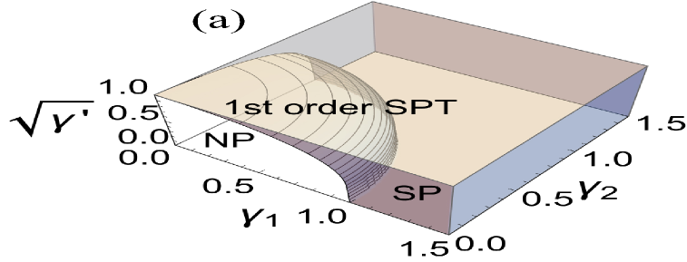
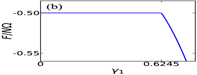
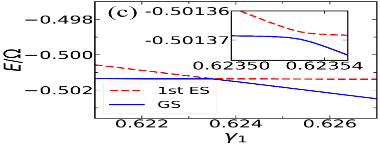
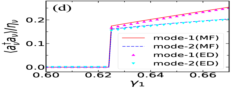
  FIG. 1: (a) The phase diagram of two-mode Dicke model with both one- and two-photon terms depicted from the phase boundary at $T=0$ in the thermodynamic limit. (b) The reduced free energy as the function of $\gamma_{1}$ plotted numerically in the classical oscillator limit for finite $N$ where the critical value $\gamma_{1c}=0.6245$, $\gamma_{2}=0.6$, and $\gamma^{\prime}_{1}=\gamma^{\prime}_{2}=0.5$. (c) The ground state (GS) and the first excited state (1st ES) energies as a function of $\gamma_{1}$ numerically obtained by exact diagonalization (ED) for $N=1$ at the finite frequency ratios $\eta_{1}=200$, $\eta_{2}=180$. The inset shows an avoided level-crossing in the neighbourhood of the critical point. (d) The rescaled mean photon number of the GS for two modes numerically obtained from mean-field method (MF) and ED, respectively.

We also obtain the solution $u_{1c}=\gamma_{1}\gamma^{\prime}/(1-\gamma^{\prime 2})$ to Eq. (21) implying $|\vec{z}_{c}|\neq 0$ at the boundary $\gamma^{2}+\gamma^{\prime 2}=1$, no matter how vanishingly small $\gamma^{\prime}$ is as long as $\gamma^{\prime}\neq 0$. It means that the rescaled mean photon number (first derivative of the reduced free energy) is discontinuous at the phase transition point, and the SPT is $1st$ order. However, when $\gamma^{\prime}$ increases smoothly from zero to nonzero, the rescaled mean photon number undergoes a continuous change and the SPT is $2nd$ order. This is because the addition of the two-photon term leads to the $Z_{2}$ symmetry breaking (Ying et al., 2020).

We draw the phase diagram of two-mode QRM with both one- and two-photon terms to show the general phase diagram feature that a SPT radially occurs along $\vec{\lambda}=(\gamma_{1},\gamma_{2},\sqrt{\gamma^{\prime}})$ under the stability condition in Fig. 1. Figure 1 shows the free energy per qubit in the unit of $\Omega$, plotted by numerically finding the global minima of the Landau potential Eq. (18) with respect to $\gamma_{1}$. The discontinuity of the first derivative of free energy implies a $1st$ order phase transition, testified by the exact diagonalization at finite frequency ratios $\eta_{1}=200$, $\eta_{2}=180$, as shown in Fig. 1, where the sharp avoided crossing brings discontinuity when $\eta_{1,2}\to\infty$. Meanwhile, the cavity field in the ground state acquires a macroscopic population of photons [see Fig. 1]. The result of ED coincides with that obtained by finding the minimum of Landau potential Eq. (18). We also numerically calculate the ratio of the rescaled mean photon number between two modes in the SP and find it consistent with Eq. (20). Here, the Fock subspace of each field mode is truncated at $N_{\mathrm{cut}}=100$ to realize the convergence of the ground state.

IV Rabi-Stark-Hubbard model

Besides the one- and two-photon coupling processes, we also study the effects of the nonlinear Stark coupling and inter-cavity hopping on the phase diagram. To this end, we consider one-dimensional Rabi-Stark-Hubbard model, describing a chain of cascaded cavities with $M$ sites where each cavity is labelled with index $i$ and governed by Rabi-Stark model. The adjacent cavities are coupled though photon couplings. This Hamiltonian corresponds to Eq. (1) without the third and fifth lines, which reads

$$H=\sum^{M}_{j}{H^{\mathrm{RS}}_{j}}-J\sum^{M}_{j}{(a_{j}+a^{{\dagger}}_{j})(a_{j+1}+a^{{\dagger}}_{j+1})},$$ (22)

where

$$H^{\mathrm{RS}}_{j}=\omega a^{{\dagger}}_{j}a_{j}+(\frac{\Omega}{2}+Ua^{{\dagger}}_{j}a_{j})\sigma^{z}_{j}+g(a_{j}+a^{{\dagger}}_{j})\sigma^{x}_{j}.$$ (23)

Here, $U$ and $J$ represent the strength of the Stark shift (Grimsmo and Parkins, 2013) and inter-cavity hopping, respectively. The stability condition of the system is $1-4J/\omega-U/\omega>0$, which will be discussed later. Employing the decoupling approximation (Greentree et al., 2006) $a_{j}a^{{\dagger}}_{j+1}\approx a_{j}\psi^{*}+a^{{\dagger}}_{j+1}\psi-|\psi|^{2}$ where the coherent field $\langle a_{j}\rangle=\psi$ is the expectation value of $a_{j}$ in terms of the stable state, we obtain a decoupled Hamiltonian:

$$H\approx\sum^{M}_{j}{H^{\mathrm{eff}}_{j}},$$ (24)

where

$$H^{\mathrm{eff}}_{j}=H^{\mathrm{RS}}_{j}-J[2(a_{j}+a^{{\dagger}}_{j})(\psi+\psi^{*})-2|\psi|^{2}-\psi^{2}-\psi^{*2}].$$ (25)

We focus on the on-site effective Hamiltonian $H^{\mathrm{eff}}_{j}$ and consider the classical oscillator limit $\eta=\Omega/\omega\rightarrow\infty$. The rescaled Hamiltonian reads

$$H^{\mathrm{eff}}_{j}/\Omega = (\frac{1}{2}+\frac{U}{\omega}\frac{a^{{\dagger}}_{j}a_{j}}{\eta})\sigma^{z}_{j}+\frac{g}{\sqrt{\Omega\omega}}(\frac{a_{j}}{\sqrt{\eta}}+\frac{a^{{\dagger}}_{j}}{\sqrt{\eta}})\sigma^{x}_{j}$$ (26)

$$+\frac{a^{{\dagger}}_{j}a_{j}}{\eta}-\frac{2J}{\omega}(\frac{a_{j}}{\sqrt{\eta}}+\frac{a^{{\dagger}}_{j}}{\sqrt{\eta}})(\frac{\psi}{\sqrt{\eta}}+\frac{\psi^{*}}{\sqrt{\eta}})$$

$$+\frac{2J}{\omega}\frac{|\psi|^{2}}{\eta}+\frac{J}{\omega}(\frac{\psi^{2}}{\eta}+\frac{\psi^{*2}}{\eta}).$$

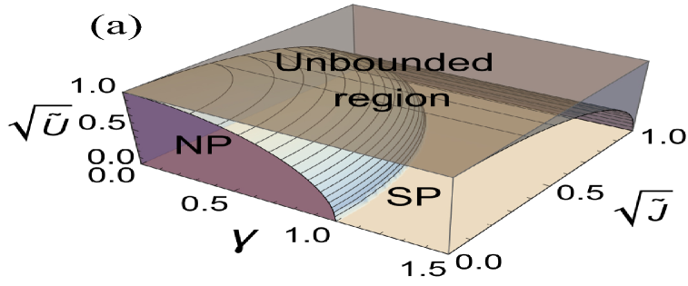
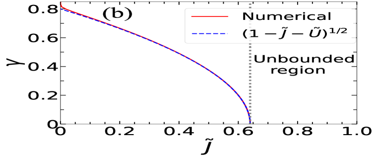
  FIG. 2: (a) Phase diagram of the on-site effective Hamiltonian in the classical oscillator limit and at zero temperature, where the surface between the NP region and the SP region represents a $2nd$ order SPT. (b) Phase boundary of the on-site effective Hamiltonian of the model at zero temperature with $\tilde{U}=0.36$ and $\Omega/\omega=400$. The region below (above) the border represents the NP (SP). There is an unbounded region for $\tilde{J}>0.64$. The red line is obtained with the self-consistent method in Ref. (Schiró et al., 2013). The dashed blue line is obtained with our method. They coincide with each other in the classical oscillator limit.

Applying the same method in the previous section, we obtain the Landau potential for $H^{\mathrm{eff}}_{j}$

$$\phi(u,v) = -\frac{1}{2}\sqrt{[1+2\tilde{U}(u^{2}+v^{2})]^{2}+4\gamma^{2}u^{2}}$$ (27)

$$+(1-\tilde{J})u^{2}+v^{2},$$

where we omit the subscript $j$ for convenience. Here, the coupling parameter settings are $\tilde{U}=U/\omega$, $\tilde{J}=4J/\omega$, and $\gamma=2g/\sqrt{\Omega\omega}$. The real and imaginary parts of $\psi/\sqrt{\eta}$ are denoted by $u$ and $v$, respectively.

We next briefly discuss the stability of this model by studying the on-site Landau potential. Considering that the quartic terms of $u$ and $v$ with coefficient $\tilde{U}^{2}$ are leading-order within the square root in Eq. (27), the stability of the system consequently requires $1-\tilde{J}-\tilde{U}>0$ for the Landau potential to have a lower bound. Due to the fact that the Landau potential Eq. (27) with specific $\vec{z}=(u,v)$ and $\vec{\lambda}=(\gamma,\tilde{J}^{1/2},\tilde{U}^{1/2})$ satisfies Eq. (2) formally, the phase diagram of this model is predicted to exhibit the above-mentioned general feature. Since the phase diagram is determined by the GMLP, we need to find the minima of the Landau potential, which satisfy

$$\frac{\partial\phi}{\partial u} =2u\left\{1-\tilde{J}-\frac{[1+2\tilde{U}(u^{2}+v^{2})]\tilde{U}+\gamma^{2}}{\sqrt{[1+2\tilde{U}(u^{2}+v^{2})]^{2}+4\gamma^{2}u^{2}}}\right\}=0,$$ (28)

$$\frac{\partial\phi}{\partial v} =2v\left\{1-\frac{[1+2\tilde{U}(u^{2}+v^{2})]\tilde{U}}{\sqrt{[1+2\tilde{U}(u^{2}+v^{2})]^{2}+4\gamma^{2}u^{2}}}\right\}=0.$$ (29)

Obviously, the GMLP is located at the origin $(u,v)=0$ when $|\vec{\lambda}|$ approaches zero. Considering $\tilde{U}<1-\tilde{J}$, the expression in the curly brace in Eq. (29) is always positive, meaning that there is no nonzero solution to Eq. (29) so that we can neglect the imaginary part. The Landau potential can be rewritten as

$$\phi(u)=(1-\tilde{J})u^{2}-\frac{1}{2}\sqrt{(1+2\tilde{U}u^{2})^{2}+4\gamma^{2}u^{2}}.$$ (30)

Considering that it is still complicate to determine the minimum by taking the derivative, we choose to solve $\phi(u\neq 0)=\phi(0)$. We find that nonzero solutions exist for $\gamma^{2}+\tilde{J}+\tilde{U}>1$ under the stability condition. Hence the phase boundary is identified as $\gamma^{2}+\tilde{J}+\tilde{U}-1=0$. In addition, the expression of nonzero solutions reads

$$u^{2}=\frac{\gamma^{2}+\tilde{J}+\tilde{U}-1}{(1-\tilde{J}+\tilde{U})(1-\tilde{J}-\tilde{U})},$$ (31)

which tends to zero at the phase boundary, indicating a $2nd$ order SPT because the change of the order parameter $u^{2}$ is continuous from the NP to the SP. It is worth noting that the general phase diagram feature is well reflected in the boundary $|\vec{\lambda}|^{2}=1$. We draw the phase diagram by finding the GLMP of the Landau potential Eq. (30). The general feature is straightforward, as shown in Fig. 2.

Another way to calculate the phase boundary without taking the classical oscillator limit is to determine $\psi=\langle a\rangle$ self-consistently (Schiró et al., 2013), where $\langle a\rangle$ is the mean value of $a$ in the ground state of the single site effective Hamiltonian Eq. (25), which gives

$$\frac{1}{\tilde{J_{\mathrm{c}}}}=\omega\sum_{n}|\langle n|a+a^{{\dagger}}|\mathrm{GS}\rangle|^{2}\frac{1}{E_{n}-E_{\mathrm{g}}},$$ (32)

where $|\mathrm{GS}\rangle$ and $|n\rangle$ are the ground and excited states of the on-site Rabi-Stark Hamiltonian with energies $E_{\mathrm{g}}$ and $E_{n}$, respectively. As a function of $\gamma$, the right hand side of Eq. (32) can be numerically obtained by exact diagonalization of the Rabi-Stark Hamiltonian. We compare this result with the classical oscillator mean field result and find that they are well consistent when $\eta\rightarrow\infty$, as shown in Fig. 2. Therefore, our method works well in the classical oscillator limit.

V Anisotropic Rabi-Stark model

Finally, we consider the anisotropic couplings. To investigate the effects of anisotropy on the phase diagram feature, we consider the anisotropic Rabi-Stark model in the classical oscillator limit for $U<\omega$. It should be pointed out that the quantum phase transitions of the anisotropic Rabi-Stark model have been studied by Xie et al. (Xie et al., 2020) at $|U|=\omega$ for the finite frequency ratio case. The Hamiltonian corresponds to the first four terms with $M=N=1$ in Eq. (1), which reads

$$H = g_{1}(a^{{\dagger}}\sigma^{-}+a\sigma^{+})+g_{2}(a\sigma^{-}+a^{{\dagger}}\sigma^{+})$$ (33)

$$+\omega a^{{\dagger}}a+\left(\frac{\Omega}{2}+Ua^{{\dagger}}a\right)\sigma^{z},$$

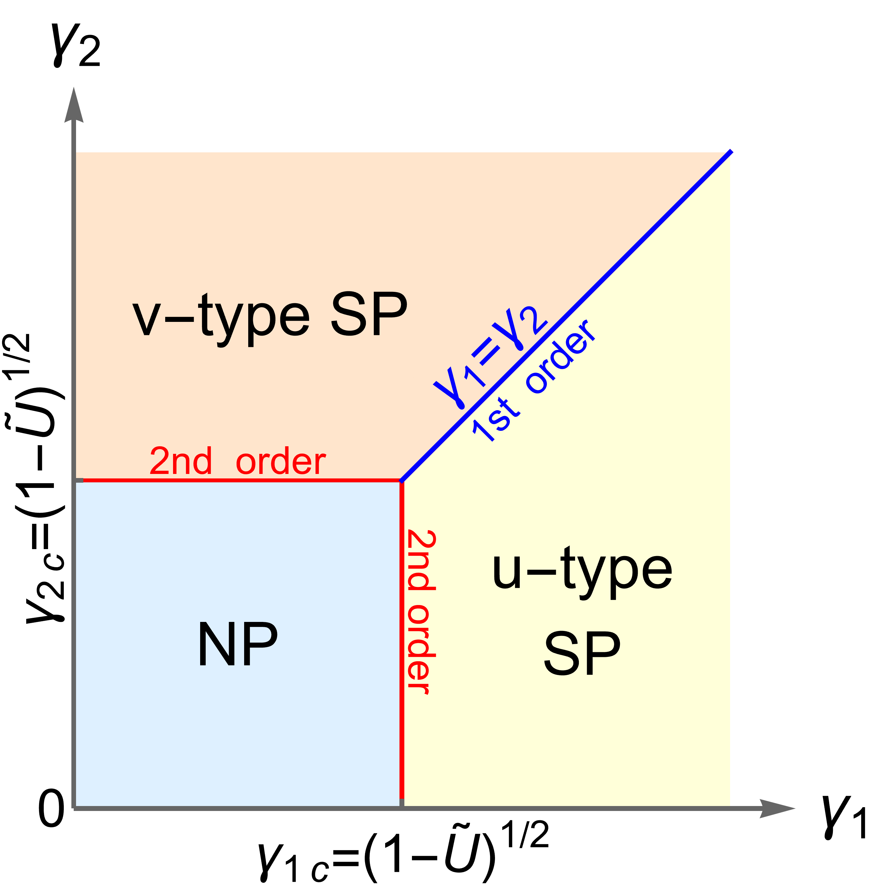
  FIG. 3: Phase diagram of the model in the classical oscillator limit $\Omega/\omega\rightarrow\infty$ at zero temperature.

where $g_{1}$ and $g_{2}$ are the coupling parameters for the rotating-wave term and counter-rotating term, respectively. The Hamiltonian in Eq. (33) possesses a $Z_{2}$ symmetry. There exists a parity operator $\Pi=\exp[\mathrm{i}\pi(a^{{\dagger}}a+\sigma^{+}\sigma^{-})]$ satisfying $[\Pi,H]=0$. Following the previous approaches developed, the Landau potential at zero temperature is derived as

$$\phi(u,v) = -\frac{1}{2}\sqrt{[1+2\tilde{U}(u^{2}+v^{2})]^{2}+4\gamma^{2}_{1}u^{2}+4\gamma^{2}_{2}v^{2}}$$ (34)

$$+u^{2}+v^{2},$$

where $\gamma_{1}=(g_{1}+g_{2})/\sqrt{\Omega\omega}$, $\gamma_{2}=(g_{1}-g_{2})/\sqrt{\Omega\omega}$, and $\tilde{U}=U/\omega$ are the dimensionless coupling constants. Similarly, Eq. (34) has the form of Eq. (2) if $\vec{z}=(u,v)$ and $\vec{\lambda}=(\gamma_{1},\gamma_{2},\tilde{U}^{1/2})$ are identified. Therefore, the general phase diagram feature still holds. In addition, the stability condition $\tilde{U}<1$ should be satisfied to ensure that the Landau potential is bounded from below. Subsequently, we start to discuss the minima of the Landau potential:

$$\frac{\partial\phi}{\partial u} =2u\left\{1\!-\!\frac{[1+2\tilde{U}(u^{2}+v^{2})]\tilde{U}+\gamma^{2}_{1}}{\sqrt{[1\!+\!2\tilde{U}(u^{2}\!+\!v^{2})]^{2}\!+\!4(\gamma^{2}_{1}u^{2}\!+\!\gamma^{2}_{2}v^{2})}}\right\}\!=\!0,$$ (35)

$$\frac{\partial\phi}{\partial v} =2v\left\{1\!-\!\frac{[1+2\tilde{U}(u^{2}+v^{2})]\tilde{U}+\gamma^{2}_{2}}{\sqrt{[1\!+\!2\tilde{U}(u^{2}\!+\!v^{2})]^{2}\!+\!4(\gamma^{2}_{1}u^{2}\!+\!\gamma^{2}_{2}v^{2})}}\right\}\!=\!0.$$ (36)

Apparently, $\phi(0,0)$ is the global minimum as $|\vec{\lambda}|$ is close to zero. The ratio of $\gamma_{1}$ to $\gamma_{2}$ determines which equation has nonzero solutions. When $\gamma_{1}=\gamma_{2}=\gamma$, Eqs. (35) and (36) become completely identical in form. It follows that $u$ and $v$ equally contribute to the rescaled mean photon number.

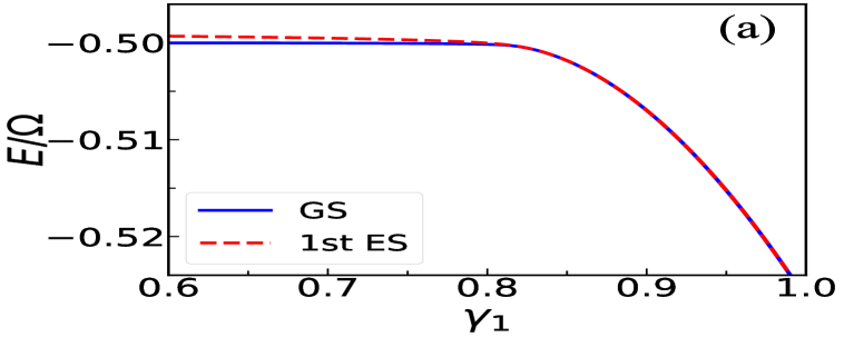
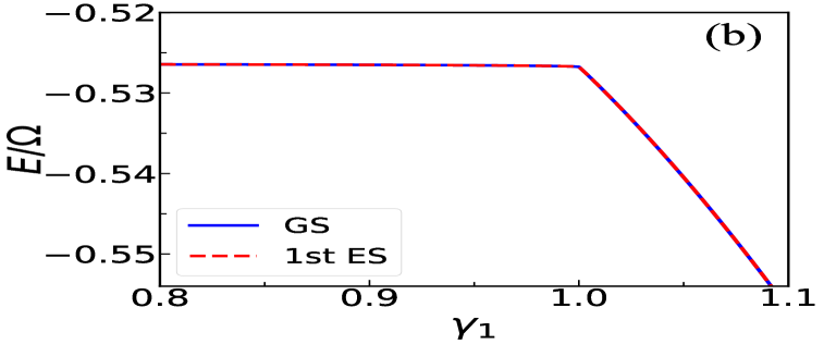
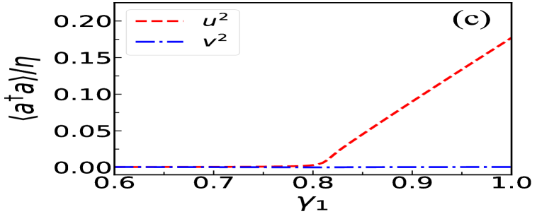
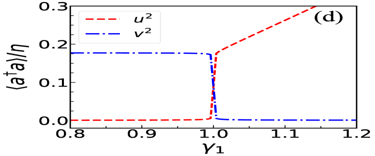
  FIG. 4: The energies in the ground state (GS) and the first excited state (1st ES) as a function of $\gamma_{1}$ for (a) $\gamma_{2}=0.6$, (b) $\gamma_{2}=1$. The rescaled mean photon number in the ground state as a function of $\gamma_{1}$ for (c) $\gamma_{2}$=0.6, (d) $\gamma_{2}$=1. Here, $\langle a^{{\dagger}}a\rangle/\eta=u^{2}+v^{2}$, $\Omega/\omega=400$ and $\tilde{U}=0.36$.

By solving $\phi(u,v)=\phi(0,0)$, we find that nonzero solutions

$$u^{2}+v^{2}=\frac{\gamma^{2}+\tilde{U}-1}{(1-\tilde{U})(1+\tilde{U})}$$ (37)

exists when $\gamma^{2}+\tilde{U}-1>0$. This indicates a $2nd$ order SPT because the change of the order parameter $u^{2}+v^{2}$ is continuous at the phase boundary $\gamma^{2}+\tilde{U}-1=0$, i.e., $|\vec{\lambda}|=1$. The boundary can be reduced to that in the Jaynes-Cummings model if $\tilde{U}=0$. In the same way, we obtain the phase boundaries $\gamma^{2}_{1}+\tilde{U}-1=0$ for $\gamma_{1}/\gamma_{2}>1$ and $\gamma^{2}_{2}+\tilde{U}-1=0$ for $\gamma_{2}/\gamma_{1}>1$. And we find two distinct $Z_{2}$ symmetry breaking SPs, each of which has a rescaled mean photon number in the ground state depending solely on $u$ or $v$. We call them $u$-type SP and $v$-type SP, respectively. We also find that the phase transitions from the NP to both SPs are $2nd$ order while the quantum phase transition between two SPs is $1st$ order. Based on the analysis above, we draw the phase diagram of the model in the ($\gamma_{1}$, $\gamma_{2}$) plane in Fig. 4. The phase diagram has a similar structure to that in Ref. (Baksic and Ciuti, 2014), with the difference that the critical coupling values are associated with $\tilde{U}$ here. It is worth pointing out that despite the presence of two SPs, the general phase diagram feature of the system entering the SP from the NP radially in the coupling parameter space is still preserved.

To confirm the validity of our analysis on the phase diagram, we numerically calculate the low energy spectrum and the rescaled mean photon number in the ground state at certain values of $\tilde{U}$ and $\gamma_{2}$, as shown in Fig. 4. In Fig. 4, the ground state and the first excited state are not approximately degenerate until $\gamma_{1}$ reaches the $2nd$ order phase transition point $\gamma_{1c}=0.8$. The appearance of the degeneracy implies the $Z_{2}$ symmetry breaking. The continuous change of the $u$-dependant rescaled mean photon number at the critical point indicates that the transition from the NP to the $u$-type SP is a $2nd$ order SPT, as shown in Fig. 4. In Fig. 4, since $\gamma_{2}=1>\gamma_{2c}$, the system is always in the SP and this can be verified by the degeneracy between two lowest energy states. Moreover, the sharp decrease of the ground state energy in the limit of $\eta\rightarrow\infty$ lead to the discontinuity of its first-order derivative, which signals the emergence of a $1st$ order quantum phase transition. The abrupt changes of $u^{2}$ and $v^{2}$ indicate that system undergoes a $1st$ quantum phase transition from the $v$-type SP to the $u$-type SP in Fig. 4.

To this end, we confirm the general light-matter interaction model Eq. (1) has the phase diagram feature we found, since the last line regarding qubit-qubit interaction generally will not change the general form of Landau potential Eq. (2).

VI Conclusions

We find a general phase diagram feature of light-matter systems describing that by specifically choosing a coupling parameter vector $\vec{\lambda}$, the systems are in NP at the origin of the coupling parameter space, and they go to SP radially and stay there afterwards. We can obtain the phase boundary and determine the rescaled mean photon number there with a concise method, so that one can identify whether SPT exists and is first-order or second-order. We illustrate this result with the multimode Dicke model with both one- and two-photon terms, the Rabi-Stark-Hubbard model, and the anisotropic Rabi-Stark model. We find the addition of photon modes will reduce the coupling strength requirement on each mode for SPT, even to the strong coupling regime. Our work provides a insight into studying and understanding the phase diagrams of the SPT.

*

Appendix A The stability condition of multimode Dicke model with both one- and two-photon terms

The stability condition can be determined by ensuring that the Landau potential is lower bounded. Here, we apply a brief analysis to the Landau potential in Eq. (10) in the main text. The Landau potential at zero temperature is rewritten as

$$\phi(\vec{z})=\sum^{M}_{\nu=1}{(u^{2}_{\nu}+v^{2}_{\nu})}-\frac{1}{2}\sqrt{1+\xi^{2}},$$ (38)

with $\xi=2\sum^{M}_{\nu=1}{[\gamma_{\nu}u_{\nu}+\gamma^{\prime}_{\nu}(u^{2}-v^{2})]}$. To consider the asymptotic behavior at $u,v\gg 1$, we approximate the Landau potential as

$$\phi(\vec{z})_{\pm}=\sum^{M}_{\nu=1}{\phi(u_{\nu},v_{\nu})_{\pm}},$$ (39)

with

$$\phi(u_{\nu},v_{\nu})_{\pm} = (1\mp\gamma^{\prime}_{\nu})\left[u\mp\frac{\gamma_{\nu}}{2(1\mp\gamma^{\prime}_{\nu})}\right]^{2}-\frac{\gamma^{2}_{\nu}}{4(1\mp\gamma^{\prime}_{\nu})}$$ (40)

$$+(1\pm\gamma^{\prime}_{\nu})v^{2}_{\nu}.$$

The subscripts of $\phi(u_{\nu},v_{\nu})_{\pm}$ depend on whether $\xi$ takes the positive or negative sign. The Landau potential $\phi(u_{\nu},v_{\nu})_{\pm}$ is quadratic and the condition $\gamma^{\prime}_{\nu}<1$ must be required to ensure that $\phi(u_{\nu},v_{\nu})_{\pm}$ is bounded from below both in the $u$ and $v$ plane.

References

- Dicke (1954) R. H. Dicke, Phys. Rev. 93, 99 (1954).
- Hepp and Lieb (1973) K. Hepp and E. H. Lieb, Ann. Phys. (N. Y.) 76, 360 (1973).
- Wang and Hioe (1973) Y. K. Wang and F. T. Hioe, Phys. Rev. A 7, 831 (1973).
- Emary and Brandes (2003) C. Emary and T. Brandes, Phys. Rev. E 67, 066203 (2003).
- Bakemeier et al. (2012) L. Bakemeier, A. Alvermann, and H. Fehske, Phys. Rev. A 85, 043821 (2012).
- Ashhab (2013) S. Ashhab, Phys. Rev. A 87, 013826 (2013).
- Hwang et al. (2015) M.-J. Hwang, R. Puebla, and M. B. Plenio, Phys. Rev. Lett. 115, 180404 (2015).
- Hwang and Plenio (2016) M.-J. Hwang and M. B. Plenio, Phys. Rev. Lett. 117, 123602 (2016).
- Liu et al. (2017) M. Liu, S. Chesi, Z.-J. Ying, X. Chen, H.-G. Luo, and H.-Q. Lin, Phys. Rev. Lett. 119, 220601 (2017).
- Forn-Díaz et al. (2010) P. Forn-Díaz, J. Lisenfeld, D. Marcos, J. J. García-Ripoll, E. Solano, C. J. P. M. Harmans, and J. E. Mooij, Phys. Rev. Lett. 105, 237001 (2010).
- Niemczyk et al. (2010) T. Niemczyk, F. Deppe, H. Huebl, E. P. Menzel, F. Hocke, M. J. Schwarz, J. J. Garcia-Ripoll, D. Zueco, T. Hümmer, E. Solano, A. Marx, and R. Gross, Nat. Phys. 6, 772 (2010).
- Ballester et al. (2012) D. Ballester, G. Romero, J. J. García-Ripoll, F. Deppe, and E. Solano, Phys. Rev. X 2, 021007 (2012).
- Bayer et al. (2017) A. Bayer, M. Pozimski, S. Schambeck, D. Schuh, R. Huber, D. Bougeard, and C. Lange, Nano Lett. 17, 6340 (2017).
- Casanova et al. (2010) J. Casanova, G. Romero, I. Lizuain, J. J. García-Ripoll, and E. Solano, Phys. Rev. Lett. 105, 263603 (2010).
- Yoshihara et al. (2017) F. Yoshihara, T. Fuse, S. Ashhab, K. Kakuyanagi, S. Saito, and K. Semba, Nat. Phys. 13, 44 (2017).
- Dimer et al. (2007) F. Dimer, B. Estienne, A. S. Parkins, and H. J. Carmichael, Phys. Rev. A 75, 013804 (2007).
- Baden et al. (2014) M. P. Baden, K. J. Arnold, A. L. Grimsmo, S. Parkins, and M. D. Barrett, Phys. Rev. Lett. 113, 020408 (2014).
- (18) J.-F. Huang and L. Tian, arXiv: 2208.12524 .
- Baumann et al. (2010) K. Baumann, C. Guerlin, F. Brennecke, and T. Esslinger, Nature 464, 1301 (2010).
- Baumann et al. (2011) K. Baumann, R. Mottl, F. Brennecke, and T. Esslinger, Phys. Rev. Lett. 107, 140402 (2011).
- De Bernardis et al. (2018) D. De Bernardis, T. Jaako, and P. Rabl, Phys. Rev. A 97, 043820 (2018).
- Araújo et al. (2016) M. O. Araújo, I. Krešić, R. Kaiser, and W. Guerin, Phys. Rev. Lett. 117, 073002 (2016).
- Roof et al. (2016) S. J. Roof, K. J. Kemp, M. D. Havey, and I. M. Sokolov, Phys. Rev. Lett. 117, 073003 (2016).
- Viehmann et al. (2011) O. Viehmann, J. von Delft, and F. Marquardt, Phys. Rev. Lett. 107, 113602 (2011).
- Zhang et al. (2014) Y. Zhang, L. Yu, J. Q. Liang, G. Chen, S. Jia, and F. Nori, Sci. Rep. 4, 4083 (2014).
- Bamba et al. (2016) M. Bamba, K. Inomata, and Y. Nakamura, Phys. Rev. Lett. 117, 173601 (2016).
- Tighineanu et al. (2016) P. Tighineanu, R. S. Daveau, T. B. Lehmann, H. E. Beere, D. A. Ritchie, P. Lodahl, and S. Stobbe, Phys. Rev. Lett. 116, 163604 (2016).
- DeVoe and Brewer (1996) R. G. DeVoe and R. G. Brewer, Phys. Rev. Lett. 76, 2049 (1996).
- Genway et al. (2014) S. Genway, W. Li, C. Ates, B. P. Lanyon, and I. Lesanovsky, Phys. Rev. Lett. 112, 023603 (2014).
- Puebla et al. (2017) R. Puebla, M.-J. Hwang, J. Casanova, and M. B. Plenio, Phys. Rev. Lett. 118, 073001 (2017).
- Gambetta et al. (2019) F. M. Gambetta, I. Lesanovsky, and W. Li, Phys. Rev. A 100, 022513 (2019).
- Cai et al. (2021) M. L. Cai, Z. D. Liu, W. D. Zhao, Y. K. Wu, Q. X. Mei, Y. Jiang, L. He, X. Zhang, Z. C. Zhou, and L. M. Duan, Nat. Commun. 12, 1126 (2021).
- Chen et al. (2015) Y. Chen, H. Zhai, and Z. Yu, Phys. Rev. A 91, 021602 (2015).
- Zhang et al. (2021a) X. Zhang, Y. Chen, Z. Wu, J. Wang, J. Fan, S. Deng, and H. Wu, Science 373, 1359 (2021a).
- Baksic and Ciuti (2014) A. Baksic and C. Ciuti, Phys. Rev. Lett. 112, 173601 (2014).
- Xie et al. (2020) Y.-F. Xie, X.-Y. Chen, X.-F. Dong, and Q.-H. Chen, Phys. Rev. A 101, 053803 (2020).
- Jiang et al. (2021) X. Jiang, B. Lu, C. Han, R. Fang, M. Zhao, Z. Ma, T. Guo, and C. Lee, Phys. Rev. A 104, 043307 (2021).
- Zhang et al. (2021b) Y.-Y. Zhang, Z.-X. Hu, L. Fu, H.-G. Luo, H. Pu, and X.-F. Zhang, Phys. Rev. Lett. 127, 063602 (2021b).
- Felicetti et al. (2015) S. Felicetti, J. S. Pedernales, I. L. Egusquiza, G. Romero, L. Lamata, D. Braak, and E. Solano, Phys. Rev. A 92, 033817 (2015).
- Duan et al. (2016) L. Duan, Y.-F. Xie, D. Braak, and Q.-H. Chen, J. Phys. A: Math. Theor. 49, 464002 (2016).
- Garbe et al. (2017) L. Garbe, I. L. Egusquiza, E. Solano, C. Ciuti, T. Coudreau, P. Milman, and S. Felicetti, Phys. Rev. A 95, 053854 (2017).
- Chen and Zhang (2018) X.-Y. Chen and Y.-Y. Zhang, Phys. Rev. A 97, 053821 (2018).
- Cong et al. (2019) L. Cong, X.-M. Sun, M. Liu, Z.-J. Ying, and H.-G. Luo, Phys. Rev. A 99, 013815 (2019).
- Lo (2020) C. F. Lo, Sci. Rep. 10, 18761 (2020).
- Greentree et al. (2006) A. D. Greentree, C. Tahan, J. H. Cole, and L. C. L. Hollenberg, Nat. Phys. 2, 856 (2006).
- Lei and Lee (2008) S.-C. Lei and R.-K. Lee, Phys. Rev. A 77, 033827 (2008).
- Schiró et al. (2012) M. Schiró, M. Bordyuh, B. Öztop, and H. E. Türeci, Phys. Rev. Lett. 109, 053601 (2012).
- Schiró et al. (2013) M. Schiró, M. Bordyuh, B. Öztop, and H. E. Türeci, J. Phys. B: At., Mol. Opt. Phys 46, 224021 (2013).
- Wang et al. (2020) Y. Wang, M. Liu, W.-L. You, S. Chesi, H.-G. Luo, and H.-Q. Lin, Phys. Rev. A 101, 063843 (2020).
- Alderete and Rodríguez-Lara (2016) C. H. Alderete and B. M. Rodríguez-Lara, J. Phys. A: Math. Theor. 49, 414001 (2016).
- Shen et al. (2021) L.-T. Shen, J.-W. Yang, Z.-R. Zhong, Z.-B. Yang, and S.-B. Zheng, Phys. Rev. A 104, 063703 (2021).
- Soldati et al. (2021) R. R. Soldati, M. T. Mitchison, and G. T. Landi, Phys. Rev. A 104, 052423 (2021).
- Devi et al. (2020) A. Devi, S. D. Gunapala, M. I. Stockman, and M. Premaratne, Phys. Rev. A 102, 013701 (2020).
- Xie et al. (2019) Y.-F. Xie, L. Duan, and Q.-H. Chen, Phys. Rev. A 99, 013809 (2019).
- Peng et al. (2019) J. Peng, E. Rico, J. X. Zhong, E. Solano, and I. L. Egusquiza, Phys. Rev. A 100, 063820 (2019).
- Cui et al. (2019) S. Cui, F. Hébert, B. Grémaud, V. G. Rousseau, W. Guo, and G. G. Batrouni, Phys. Rev. A 100, 033608 (2019).
- Cui et al. (2020) S. Cui, B. Grémaud, W. Guo, and G. G. Batrouni, Phys. Rev. A 102, 033334 (2020).
- Ying et al. (2020) Z.-J. Ying, L. Cong, and X.-M. Sun, J. Phys. A: Math. Theor. 53, 345301 (2020).
- He et al. (2022) S. He, L.-W. Duan, Y.-Z. Wang, C. Wang, and Q.-H. Chen, Phys. Rev. A 106, 033712 (2022).
- Felicetti and Le Boité (2020) S. Felicetti and A. Le Boité, Phys. Rev. Lett. 124, 040404 (2020).
- (61) J. Peng, E. Rico, J. X. Zhong, E. Solano, and I. L. Egusquiza, arXiv:1904.02118 .
- Grimsmo and Parkins (2013) A. L. Grimsmo and S. Parkins, Phys. Rev. A 87, 033814 (2013).