Quantifying Coherence and Genuine Multipartite Entanglement : A Framework Based on Witness Operators and Frobenius Norm Distance

Abstract

Quantifying the entanglement and coherence of quantum systems is a topic of significant theoretical and practical interest. In this paper, we propose a method to evaluate lower bounds for several widely used coherence measures and genuine multipartite entanglement (GME) measures. Our approach, which is resource-efficient and computationally feasible, provides bounds of coherence and GME measures with the help of witnesses by the $F$-norm. Finally, we present a practical framework for estimating these quantum resources in various physical scenarios.

I Introduction

Quantum advantage refers to the capability of quantum computers to surpass classical computers in performing certain tasks Harrow2017 . Quantum entanglement and quantum coherence are two crucial quantum resources RevModPhys.91.025001 that establish this advantage. For instance, Shor’s algorithm Shor1995PolynomialTimeAF utilizes an entangled chain to solve the problem of large integer factorization, while Grover’s algorithm 10.1145/237814.237866 relies on maintaining coherent operations to ensure success rates. In some recent quantum application achievements, efforts have also been made to reduce the consumption of these two quantum resources. For example, a new quantum processor architecture Stassi2020 was proposed, significantly enhancing qubit coherence time and operational precision. Similarly, a quantum error-correcting code PhysRevA.111.012444 was introduced, substantially reducing the entanglement overhead of physical qubits.

Quantum entanglement is one of the most famous non-classical phenomena in quantum mechanics, characterized by strong correlations between multiple particles that transcends classical physics. Even when they are far apart, the measurement result of one particle will instantaneously affects another particle. The mathematical definition of entanglement is as follows RevModPhys.81.865 : A mixed state $\rho$ is considered separable if it can be expressed in the form:

$$\rho=\sum_{i}p_{i}\rho_{i}^{A}\otimes\rho_{i}^{B},$$ (1)

where $\rho_{i}\geq 0$ and $\sum_{i}p_{i}=1$, with $\rho^{A}$ and $\rho^{B}$ being the density matrices of subsystems $A$ and $B$, respectively. If a mixed state $\rho$ cannot be represented in the above form, it is entangled. For quantifying entanglement, several entanglement measures have been proposed for bipartite systems Horodecki2001EntanglementM ; Bruss:2002bpc ; 10.5555/2011706.2011707 ; RevModPhys.81.865 ; GUHNE20091 , such as the concurrence PhysRevA.54.3824 ; PhysRevLett.78.5022 ; PhysRevLett.80.2245 ; PhysRevA.64.052304 ; PhysRevA.64.042315 ; Badziag2001ConcurrenceIA , the G-concurrence Uhlmann2010RoofsAC ; PhysRevA.71.012318 ; Fan2002QuantifyEB ; Barnum2001MonotonesAI , the geometric measure of entanglement Barnum2001MonotonesAI ; PhysRevA.68.042307 ; PhysRevA.70.022322 , and the negativity or extensions thereof HORODECKI19961 ; PhysRevLett.77.1413 ; PhysRevA.58.883 ; PhysRevA.65.032314 ; PhysRevA.68.062304 . While the above definition is aimed at bipartite systems, the question arises: how should we define entangled states in a multipartite system? When considering an $N$-partite system, it can exhibit different classes of entanglement PhysRevA.62.062314 ; PhysRevA.65.052112 ; PhysRevLett.87.040401 . Among these, one of the strongest forms is known as genuine multipartite entanglement (GME). It is defined as follows: a multipartite quantum state that is not a convex combination of biseparable states with respect to any bipartition contains GME PhysRevLett.83.3562 ; PhysRevLett.113.100501 ; PhysRevA.84.062306 . Many criteria have been introduced for multipartite entanglement detection Streltsov_2010 ; PhysRevLett.104.210501 ; PhysRevLett.106.020405 .

Figure 1: Evaluating Lower Bounds of Coherence Measures and GME Measures through Witness Operators. Where $D_{inc}$ and $D_{sep}$ are the minimum distances in terms of $F$-norm between the given state and all incoherent or separable states, respectively.

Quantum coherence stems from the basic principles of quantum mechanics. In a $d$-dimensional Hilbert space $\mathcal{H}$, by selecting a basis $\{|i\rangle\}$, the density operator $\delta$ can be expressed as PhysRevLett.113.140401 :

$$\delta=\sum_{i=1}^{d}p_{i}|i\rangle\langle i|,$$ (2)

where $0\leq p_{i}\leq 1$ and $\sum_{i=1}^{d}p_{i}=1$, represents an incoherent state. Otherwise, it is known as a coherent state. Quantum coherence allows us to do things much more efficiently than classical methods can, leading to progress in areas like low-temperature thermodynamics Narasimhachar2015 ; PRXQuantum.3.040323 ; PhysRevResearch.5.043184 , quantum key distribution PhysRevA.99.062325 ; PhysRevA.109.012614 ; PhysRevLett.130.220801 , and quantum metrology PhysRevLett.96.010401 ; PhysRevA.99.022314 ; PhysRevA.94.010102 .

As quantum information science advances, there has been a surge of interest in how to quantify coherence resources PhysRevLett.113.140401 ; RevModPhys.89.041003 ; PhysRevA.93.012334 ; PhysRevLett.119.150405 ; GUO2023106611 ; PhysRevA.107.022408 . In the groundbreaking study referenced as PhysRevLett.113.140401 , Baumgratz and colleagues established a resource theory framework for measuring coherence. They proved that both $l_{1}$-norm coherence and relative entropy coherence serve as valid measures for quantifying coherence. Shortly afterwards, Streltsov and his colleagues demonstrated that the geometric measure of coherence, linked to the geometric measure of entanglement PhysRevA.68.042307 ; Streltsov_2010 , can be evaluated explicitly.

However, regardless of whether one uses coherence measures or entanglement measures, many schemes require performing a full tomography of the state to obtain all elements of the density matrices. This means that the entire process of determining the bounds of the coherence and entanglement is significantly more resource-intensive. Moreover, when dealing with GME in large-qubit systems, such as those involving 8-12 qubits, it becomes challenging to perform quantum state tomography PhysRevApplied.13.054022 . Therefore, the question of how to quantify the coherence and GME of an unknown state with fewer resources is an intriguing problem.

In this manuscript, we provide a method to evaluate the lower bounds of coherence measures and GME measures, as illustrated in Figure 1. We employ a generic entanglement witness and coherence witnesses constructed based on decoherence operations. Using these two types of witness operators and a distance based on the $F$-norm, we first establish lower bounds for three coherence measures: the $l_{1}$-norm measure, the relative entropy of coherence, and the geometric measure of coherence. Subsequently, by using the lower bound calculation of the concurrence of a GME state as an illustrative example, we prove a universal form for the lower bound of the minimal GME measure based on entanglement witnesses. At the end of the manuscript, using the proposed lower bound evaluation method, we simulate and calculate the lower bounds of various coherence measures for different initial states, as well as the lower bound of the concurrence measure for a 4-qubit GHZ state.

II Preliminary knowledge

In this section, we will first define two distances based on the $F$-norm. These distances will play crucial roles in deriving lower bounds for entanglement and coherence measures. We will then introduce three commonly used coherence measures and the concurrence of bipartite state. Finally, we will provide a method for generalizing bipartite measures to GME measures.

II.1 The distances based on the $F$-norm

First we define the distance between the mixed state $\rho_{AB}$ and the set of separable states in term of $\|\cdot\|_{F}$ as:

$$D_{sep}(\rho)=\mathop{\rm min}_{\sigma\in S}\|\rho-\sigma\|_{F},$$ (3)

where the minimum takes over all the separable states $\sigma\in Sep(A:B)$. Given the bipartite pure state $|\psi\rangle_{AB}=\sum_{i=0}^{m-1}\sqrt{\lambda_{i}}|ii\rangle$, according to Lemma 1 we have:

$$D_{sep}(|\psi\rangle) =\sqrt{1-\sum_{i}\lambda_{i}^{2}}$$ (4)

$$\geq-\frac{1}{b}Tr(W_{0}|\psi\rangle\langle\psi|),$$ (5)

where $W_{0}$ is a generic entanglement witness of $\mathcal{H}_{d}\otimes\mathcal{H}_{d}$, $\mathcal{H}$ is a finite dimensional Hilbert space and $b=\sqrt{Tr(W_{0}^{\dagger}W_{0})-\frac{(TrW_{0})^{2}}{d^{2}}}$. Similarly, we define the distance between the mixed state $\rho$ and the set of incoherent states in term of $\|\cdot\|_{F}$ as:

$$D_{inc}(\rho)=\mathop{\rm min}_{\sigma\in\mathcal{I}}\|\rho-\sigma\|_{F}.$$ (6)

where the minimum takes over all the incoherent states $\sigma\in\mathcal{I}$.

II.2 The concurrence

The concept of concurrence was introduced to quantify the degree of entanglement in a two-qubit system. It was first proposed by Wootters et al. in 1998 PhysRevLett.80.2245 . It ranges from 0 to 1, where 0 indicates no entanglement (the state is separable) and 1 indicates maximum entanglement. Wootters’s concurrence is defined with the help of the superoperator that flips the spin of a qubit. By generalizing the spin flip superoperator to a ”universal inverter,” which acts on quantum systems of arbitrary dimension, Rungta et al.PhysRevA.64.042315 introduced a convenient expression for the concurrence that facilitates subsequent calculations.

Assume $|\psi\rangle_{AB}$ is a bipartite pure state, $|\psi\rangle_{AB}=\sum_{i=0}^{m-1}\sqrt{\lambda_{i}}|ii\rangle$, the concurrence of a pure state $|\psi\rangle_{AB}$ is defined as

$$C(|\psi\rangle_{AB})=\sqrt{2(1-\mathrm{Tr}\rho_{A}^{2})}=\sqrt{2\left(1-\sum_{i}\lambda_{i}^{2}\right)},$$

where $\rho_{A}$ is the reduce density matrix of $\rho_{AB}=|\psi\rangle_{AB}\langle\psi|$. For a mixed state $\rho_{AB}$, the concurrence for a mixed state $\rho_{AB}$ is defined by the convex roof extension method,

$$C(\rho_{AB})=\mathop{\rm min}_{\{p_{i},|\phi_{i}\rangle_{AB}\}}\sum_{i}p_{i}C(|\phi_{i}\rangle_{AB}),$$ (7)

where the minimum takes over all the decompositions of $\rho_{AB}=\sum_{i}p_{i}|\phi_{i}\rangle_{AB}\langle\phi_{i}|,$ with $p_{i}\geq 0$ and $\sum p_{i}=1$.

II.3 Commonly used coherence measures

In this part, we will provide the specific mathematical expressions for the three commonly used coherence measures introduced earlier: the $l_{1}$-norm coherence, the relative entropy coherence, and the geometric measure of coherence. For arbitrary matrix, we define that $\|\mathbf{A}\|_{\text{asum}}=\sum_{i=1}^{m}\sum_{j=1}^{n}|a_{ij}|$. Assuming $\rho$ is the density matrix of the quantum state to be measured and $\mathcal{I}$ represents the set of all incoherent states, the $l_{1}$-norm measure of coherence, which can be denoted as PhysRevLett.113.140401

$$C_{l_{1}}(\rho)=\mathop{\rm min}_{\delta\in\mathcal{I}}\|\rho-\delta\|_{\text{asum}}=\sum_{i\neq j}|\rho_{i,j}|.$$ (8)

where the minimum is achieved when $\delta$ equals the completely dephased $\rho$, i.e., the diagonal matrix consisting only of the diagonal elements of $\rho$. The relative entropy coherence, which can be denoted as PhysRevLett.113.140401

$$C_{ref}(\rho)=S(\rho_{diag})-S(\rho),$$ (9)

where $S(\cdot)$ means von Neumann entropy, $\rho_{diag}$ is a diagonal matrix composed of diagonal elements of $\rho$. For a pure state $|\psi\rangle$, its coherence of formation is defined as $C_{cof}(|\psi\rangle)=S(\Delta(|\psi\rangle\langle\psi|))$ PhysRevApplied.13.054022 , which is equivalent to $C_{ref}$. Since the former applies to mixed states via the convex roof construction PhysRevLett.116.120404 ; PhysRevA.92.022124 , we will primarily use $C_{cof}$ in the following discussion. According to PhysRevLett.115.020403 , the geometric measure of coherence can be denoted as:

$$C_{g}(\rho)=1-\mathop{\rm max}_{\delta\in\mathcal{I}}F(\rho,\delta).$$ (10)

It is important to note that when it comes to quantum coherence, we tend to view the system as a whole PhysRevLett.113.140401 ; RevModPhys.89.041003 ; HU20181 ; RevModPhys.91.025001 . Therefore, in the following coherence measures, subscripts representing subsystems are not used, to emphasize this point.

II.4 Definition of GME measures

One approach to quantifying GME is to generalize measures of bipartite entanglement to multipartite systems. Considering a bipartite entanglement measure $E$, one can define a GME measure as

$$E_{GME}(|\psi\rangle)=\mathop{\rm min}_{A|\overline{A}}E_{A|\overline{A}}(|\psi\rangle),$$ (11)

for an $N$-partite pure state $|\psi\rangle$, where $A$ represents all possible bipartitions $A|\overline{A}$ of $\{1,2,\cdots,N\}$. For instance, suppose that $i_{1},i_{2},\cdots,i_{N}$ is an arbitrary order of $1,2,\cdots,N$. The subset A contains $\{i_{1},\cdots,i_{k}\}$ and $\overline{A}$ = $\{i_{k+1},\cdots,i_{N}\}$ with $1\leq k\leq N-1$, since $A$ and $\overline{A}$ are two nonempty subsets.

For any GME measure $E_{GME}(\cdot)$ applied to an arbitrary $N$-partite state $\rho$, we have

$$E_{GME}(\rho) =\inf_{\{p_{i},|\psi_{i}\rangle\}}\sum_{i}p_{i}E_{GME}(|\psi_{i}\rangle)$$ (12)

$$E_{GME}(|\psi_{i}\rangle) =\mathop{\rm min}_{A|\overline{A}}E_{A|\overline{A}}(|\psi_{i}\rangle),$$ (13)

where $A|\overline{A}$ denotes an arbitrary bipartition, the infimum takes over all the decompositions of $\rho_{A\overline{A}}=\sum_{i}p_{i}|\psi_{i}\rangle_{A\overline{A}}\langle\psi_{i}|$, with $p_{i}\geq 0$ and $\sum_{i}p_{i}=1$, and the minimum is taken over all possible bipartitions of the N-partite system.$E_{A|\overline{A}}$ means the corresponding bipartite entanglement measure between subsystem $A$ and $\overline{A}$.

III Main results

III.1 Lower bounds of coherent quantifiers based on coherent witness

According to PhysRevA.103.012409 , For any density matrix $\sigma$, we can construct a coherence witness

$$W_{1}=\Delta(\sigma)-\sigma,$$ (14)

where $\Delta$ is the dephasing operation defined as $\Delta(\sigma)=\sum_{i=1}^{d}|i\rangle\langle i|\sigma|i\rangle\langle i|$. Furthermore if $\sigma$ is just $\rho$ itself, one can directly get that

$$-\operatorname{Tr}(\rho W_{1}) =-\operatorname{Tr}\{[\Delta(\rho)-\rho]\rho\}$$

$$=\operatorname{Tr}(\rho^{2})-\operatorname{Tr}[\Delta(\rho)\rho]$$

$$=\sum_{i,j}|\langle i|\rho|j\rangle|^{2}-\sum_{i}|\langle i|\rho|i\rangle|^{2}$$

$$=\sum_{i\neq j}|\langle i|\rho|j\rangle|^{2}$$

$$=\sum_{i\neq j}|\rho_{ij}|^{2},$$

where we have used the equations $\operatorname{Tr}(\rho^{2})=\sum_{i,j}|\langle i|\rho|j\rangle|^{2}$ and $\operatorname{Tr}[\Delta(\rho)\rho]=\sum_{i}|\langle i|\rho|i\rangle|^{2}$. In other words, when $\sigma=\rho$, we have

$$D_{inc}(\rho)=-Tr(\rho W_{1}).$$ (15)

Based on Eq.(15), we can obtain the following bounds of coherence measures based on the distance $D_{inc}$. To obtain the above results, we first present the analytical expression $D_{inc}(|\psi\rangle)$ for a bipartite pure state $|\psi\rangle$.

Theorem 1 Assume $|\psi\rangle$ is a pure state $|\psi\rangle=\sum_{i=0}^{d-1}\lambda_{i}|i\rangle$, then

$$D_{inc}(|\psi\rangle) =\mathop{\rm min}_{\sigma\in I}\||\psi\rangle\langle\psi|-\sigma\|_{F}$$ (16)

$$=\sqrt{1-\sum_{i}\lambda_{i}^{4}}$$ (17)

Theorem 2 Assume $\rho$ is a mixed state, then

$$C_{l_{1}}(\rho) \geq D_{inc}(\rho),$$ (18)

$$C_{g}(\rho) \geq\frac{1}{4}D_{inc}^{2}(\rho),$$ (19)

$$C_{cof}(\rho) \geq-log(1-D_{inc}^{2}(\rho)).$$ (20)

See Appendix V for the proof of the above equation.

Figure 2: Simulation of lower bounds for three coherence measures.

III.2 Lower bounds of GME measures based on entanglement witness

In this section, we first extend the bipartite entanglement measure, the concurrence, introduced in II.2, to the GME concurrence using the method described in II.4. We then utilize a generic entanglement witness to evaluate its lower bound. Using this process as an example, we then propose a general form for evaluating GME measures based on entanglement witnesses.

III.2.1 Lower bounds of GME concurrence

A pure $N$-partite quantum state $|\psi\rangle$ is said to exhibit genuine multipartite entanglement (GME) if it cannot be expressed as a tensor product under any nontrivial bipartition, i.e.,

$$|\psi\rangle\neq|\psi_{A}\rangle\otimes|\psi_{\overline{A}}\rangle,\quad\forall\text{ bipartitions }A|\overline{A}.$$

For a mixed state $\rho$, it is genuinely multipartite entangled if it cannot be written as a convex mixture of states separable across some bipartition:

$$\rho=\sum_{i}p_{i}\rho_{A}^{i}\otimes\rho_{\overline{A}}^{i},\quad\forall\text{ bipartitions }A|\overline{A},$$

where $p_{i}$ is a probability distribution, and $\rho_{A}^{i}$ and $\rho_{\overline{A}}^{i}$ are density matrices of subsystems $A$ and $\overline{A}$, respectively. Assume that $\rho=\sum_{i}p_{i}|\psi_{i}\rangle\langle\psi_{i}|$ is the optimal decomposition for $N$-partite state $\rho$ to achieve the infimum of $C_{GME}(\rho)=\inf_{\{p_{i},|\psi_{i}\rangle\}}\sum_{i}p_{i}C_{GME}(|\psi_{i}\rangle)$. According to shi2024lower , we have $C_{BE}(\rho)\geq\sqrt{2}D_{sep}(\rho)$. For all possible bipartitions $A|\overline{A}$, we can calculate the concurrence of $\rho$:

$$C_{BE}^{(A|\overline{A})}(\rho) =\sum_{i}p_{i}C_{BE}^{(A|\overline{A})}(|\psi_{i}\rangle)$$ (21)

$$\geq\sqrt{2}D_{sep}^{(A|\overline{A})}(\rho)$$ (22)

$$\geq-\frac{\sqrt{2}}{b_{(A|\overline{A})}}TrW_{0}\rho,$$ (23)

where $W_{0}$ is generic bipartite entanglement witness for arbitrary bipartition of the whole system, $b_{(A|\overline{A})}=\sqrt{Tr(W_{0}^{\dagger}W_{0})-\frac{(TrW_{0})^{2}}{(2^{d})^{2}}}$, $d$ is the largest of the dimensions of bipartition $A$ and $\overline{A}$. See Lemma 1 for the proof. According to Eq.(12)(13)(23), we have

$$C_{GME}(\rho) =\sum_{i}p_{i}C_{GME}(|\psi_{i}\rangle)$$ (24)

$$=\sum_{i}p_{i}\mathop{\rm min}_{A|\overline{A}}C_{BE}^{(A|\overline{A})}(|\psi_{i}\rangle)$$ (25)

$$\geq\mathop{\rm min}_{A|\overline{A}}\sqrt{2}D_{sep}^{(A|\overline{A})}(\rho)$$ (26)

$$=-\frac{\sqrt{2}}{b_{max}}TrW_{0}\rho,$$ (27)

where $b_{max}=\sqrt{Tr(W_{0}^{\dagger}W_{0})-\frac{(TrW_{0})^{2}}{(2^{N-1})^{2}}}$.

III.2.2 The general form

Using the evaluation of the lower bound for GME concurrence as an illustrative example, we propose a general form for evaluating various GME measures by leveraging entanglement witnesses. Based on the analysis of several bipartite entanglement measures shi2024lower ; PhysRevApplied.13.054022 , our proposed method is applicable to, but not limited to, GME-extended measures such as the entanglement of formation, the concurrence, the geometric entanglement measure, and the G-concurrence.

Theorem 3 Let $D_{\text{sep}}(\rho)$ be the $F$-norm distance between the given $N$-partite state $\rho$ and the nearest separable state, and let

$$\mathcal{A}=\{f\mid f:\mathbb{R}\to[0,1],\\ f\text{ is monotonically increasing and convex}\}$$ (28)

For any bipartite state $\sigma$ and a given entanglement measure $E(\sigma)$ such that there exists $f\in\mathcal{A}$, $E(\sigma)\geq f(D_{\text{sep}}(\sigma))$ then the lower bound of the GME measure generalized by $E$ can be expressed as:

$$E_{GME}(\rho) \geq f\{-\frac{1}{b_{max}}Tr(W_{0}\rho)\},$$ (29)

where, $b_{max}=\sup_{A|\overline{A}}\sqrt{Tr(W_{0}^{\dagger}W_{0})-\frac{(TrW_{0})^{2}}{(2^{d})^{2}}}$, $d=\mathop{\rm max}\{\mathop{\rm Dim}(A),\mathop{\rm Dim}(\overline{A})\}$. $W_{0}$ is a generic entanglement witness.

Proof.

Assume $\rho$ is an arbitrary $N$-partite state, and $\sigma$ is an arbitrary bipartite state. When $D_{sep}(\rho)=0$, $\rho$ is a separable state, and thus the minimum value of the bipartite entanglement measure across all bipartitions is 0 PhysRevLett.78.2275 . That is, when $D_{sep}(\rho)=0$,

$$E_{GME}(\rho) =\sum_{i}p_{i}E_{GME}(|\psi_{i}\rangle)$$

$$=\sum_{i}p_{i}\mathop{\rm min}_{A|\overline{A}}E^{(A|\overline{A})}(|\psi_{i}\rangle)$$

$$=0.$$

When $D_{sep}>0$, according to Theorem 3, $E(\sigma)\geq f(D_{sep}(\sigma))$. Then we have:

$$E_{GME}(\rho) =\sum_{i}p_{i}E_{GME}(|\psi_{i}\rangle)$$

$$=\sum_{i}p_{i}\mathop{\rm min}_{A|\overline{A}}E^{(A|\overline{A})}(|\psi_{i}\rangle)$$

$$\geq\sum_{i}p_{i}f\{\mathop{\rm min}_{A|\overline{A}}D_{sep}^{(A|\overline{A})}(|\psi_{i}\rangle)\}$$

$$\geq f\{\mathop{\rm min}_{A|\overline{A}}D_{sep}^{(A|\overline{A})}(\rho)\}$$

$$=f\{-\frac{1}{b_{max}}Tr(W_{0}\rho)\},$$

The first inequality holds because $f(\cdot)$ is a monotonically increasing function, and since $f(\cdot)$ is also a convex function, the second inequality follows from Jensen’s inequality Jensen1906 . The proof of the final equality is provided in Lemma 1.   $\sqcap$$\sqcup$

III.3 Simulation calculations

In this part, we use the lower bound evaluation method proposed in this paper to perform simulation calculations for three coherence measures under different initial states, as well as the concurrence measure for the 4-qubit GHZ state.

First, we have simulated and calculated the coherence measures for multiple mixed bipartite states using Python script, as well as determined the corresponding lower bounds using the methods described in the previous sections, as shown in Figure 2. For each group, we first randomly generated a different number of pure states, mixed them into mixed states, and then proceeded with subsequent calculations. The coherence witnesses were all based on the density matrices of the mixed bipartite states themselves. The specific calculation results are shown in Table 1.

Table 1: Three coherence measures and their corresponding lower bounds

NMPS	$C_{l_{1}}$	$D_{inc}$	$C_{g}$	$\frac{1}{4}D_{inc}^{2}$	$C_{cof}$	$-log(1-D_{inc}^{2})$
$2_{a}$	1.796	0.569	0.370	0.081	0.959	0.392
$2_{b}$	1.554	0.595	0.450	0.088	0.995	0.437
$2_{c}$	2.167	0.656	0.498	0.108	1.217	0.563
$5_{a}$	0.886	0.283	0.137	0.020	0.335	0.083
$5_{b}$	0.765	0.237	0.083	0.014	0.236	0.058
$5_{c}$	1.434	0.448	0.243	0.050	0.634	0.223
$10_{a}$	0.646	0.211	0.047	0.011	0.134	0.046
$10_{b}$	1.066	0.336	0.106	0.028	0.312	0.120
$10_{c}$	0.740	0.245	0.067	0.015	0.184	0.062
$20_{a}$	0.613	0.212	0.04435	0.01120	0.125	0.046
$20_{b}$	0.734	0.236	0.055	0.014	0.161	0.057
$20_{c}$	0.471	0.153	0.027	0.006	0.076	0.024
$100$	0.324	0.107	0.01165	0.00284	0.033	0.011

Note: NMPS stands for ”number of mixed pure states,” i.e., the number of pure states contributing to the mixed state.

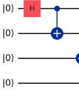
Figure 3: Generation of a 4-Qubit GHZ State.

The calculation of the GME measure is much more complicated. We will calculate the concurrence measure and its lower bound for the classical GME state, the GHZ state Greenberger1989 . First, we construct a GHZ state: Create a quantum circuit with 4 qubits, all initialized in the $|0\rangle$ state. Then, apply the H-gate (Hadamard gate) to qubit 0, followed by CNOT gates between qubit 0 and qubits 1, 2, and 3, where qubit 0 is the control qubit. The corresponding schematic of the quantum circuit is illustrated in Figure 3. This creates a 4-qubit GHZ state, which is represented by the following wavefunction:

$$|GHZ\rangle=\frac{1}{\sqrt{2}}(|0000\rangle+|1111\rangle)$$

Since the GHZ state is a maximally entangled state, the concurrence for every bipartition is 1. Therefore, its GME-concurrence value is also 1, and we can replace the overall concurrence with the concurrence of any pure state from pure state decomposition, thereby simplifying the calculation. Next, we calculate the lower bound for the GME-concurrence. We adopt the entanglement witness $W_{0}$ from PhysRevLett.92.087902 , $W_{0}=\beta\cdot I_{A}\otimes I_{\overline{A}}-|\psi\rangle\langle\psi|$, $\beta=\mathop{\rm max}_{\phi\in SEP{A:\overline{A}}}\langle\phi|\psi|\phi\rangle$. Through grid search, the maximum fidelity between this GHZ state and all possible separable states is 0.5. With $N=4$ the dimension of $I_{A}$ is 2, and the dimension of $I_{\overline{A}}$ is 8, from Eq.(27) we have

$$C_{GME}(\rho) \geq-\frac{\sqrt{2}}{b_{max}}Tr(W_{0}|\psi\rangle\langle\psi|)$$

$$\geq-\frac{\sqrt{2}}{b_{max}}(\beta-1),$$

$$b_{max}=\sqrt{Tr(W_{0}^{\dagger}W_{0})-\frac{(TrW_{0})^{2}}{(2^{N-1})^{2}}}\approx 1.7984,$$

$$C_{GME}(|GHZ\rangle)\geq-\frac{\sqrt{2}}{b_{max}}(\beta-1)\geq 0.3932$$

IV Conclusion

In this work, we have achieved two main objectives. First, we have provided lower bounds for coherence measures of mixed states using coherence witnesses. Second, we have derived lower bounds for the GME measures using entanglement witnesses. Specifically, by employing coherence witnesses constructed via decoherence operations, we have obtained the specific value of $D_{inc}$, from which we have further calculated the lower bounds for three commonly used coherence measures: the $l_{1}$-norm coherence, the relative entropy coherence, and the geometric measure of coherence. This method, which leverages witness operators and the $F$-norm distance, was initially developed to calculate lower bounds for bipartite entanglement measuresshi2024lower . Then, we have extended this lower-bound calculation method to GME measures, using concurrence as an example, and have presented a universal form applicable to all GME measures derived from bipartite measures. Compared with the method of performing the tomography of a quantum state $\rho$ to know its whole density matrix to detect and quantify the entanglement or coherence of $\rho$, this method for calculating the lower bounds has been simpler, less costly, and more practical for experimental implementation. Additionally, the lower-bound calculation approach we have proposed is not limited to quantifying entanglement and coherence as quantum resources but also has provided a research pathway for other quantum resource measures, such as quantum magic PhysRevA.71.022316 , quantum Fisher information PhysRevLett.72.3439 , and others.

V Appendix

Lemma 1

shi2024lower Assume $W_{0}$ is a generic entanglement witness of $\mathcal{H}_{d}\otimes\mathcal{H}_{d}$, let $a=\frac{\mathrm{Tr}W_{0}}{d^{2}},\quad b=\sqrt{\mathrm{Tr}(W_{0}^{\dagger}W_{0})-\frac{(\mathrm{Tr}W_{0})^{2}}{d^{2}}},\quad W_{1}=\frac{W_{0}-aI\otimes I}{b}.$ Based on the property of $\|\cdot\|_{F}$, we have

$$D_{\text{sep}}(\rho_{AB}) =\mathop{\rm min}_{\sigma\in Sep(A:B)}\mathop{\rm max}_{\|W_{1}\|_{F}=1}\mathrm{Tr}(W_{1}(\rho_{AB}-\sigma_{AB}))$$

$$\geq|\mathrm{Tr}W_{1}(\rho-\omega)|$$

$$=\left|\mathrm{Tr}\left(\frac{W_{0}}{b}(\rho-\omega)-\frac{a}{b}\mathrm{Tr}(\rho-\omega)\right)\right|$$

$$=\left|\mathrm{Tr}\left[\frac{W_{0}}{b}(\rho-\omega)\right]\right|$$

$$\geq-\frac{1}{b}\mathrm{Tr}W_{0}\rho,$$

in the first inequality, $\omega$ is the optimal separable state, $W_{1}$ is a Hermitian operator and $\|W_{1}\|_{F}=1$. The last inequality is due to $\mathrm{Tr}W_{0}\omega\geq 0$.

Lemma 2

Consider the square of the sum of the absolute values of all elements in the matrix $A\in\mathbb{R}^{m\times n}$

$$\left(\sum_{i=1}^{m}\sum_{j=1}^{n}|a_{ij}|\right)^{2}=\sum_{i=1}^{m}\sum_{j=1}^{n}|a_{ij}|^{2}+2\sum_{i<k}\sum_{j<l}|a_{ij}|\cdot|a_{kl}|.$$ (30)

Since all cross-product terms $|a_{ij}|\cdot|a_{kl}|$ are non-negative, we have:

$$\left(\sum_{i=1}^{m}\sum_{j=1}^{n}|a_{ij}|\right)^{2} \geq\sum_{i=1}^{m}\sum_{j=1}^{n}|a_{ij}|^{2}$$ (31)

$$\sum_{i=1}^{m}\sum_{j=1}^{n}|a_{ij}| \geq\sqrt{\sum_{i=1}^{m}\sum_{j=1}^{n}|a_{ij}|^{2}}$$ (32)

$$\|\mathbf{A}\|_{\text{asum}} \geq\|\mathbf{A}\|_{F}.$$ (33)

This proves that the $F$-norm of a matrix is less than or equal to the sum of the absolute values of all its elements.

Theorem 1 Assume $|\psi\rangle$ is a pure state $|\psi\rangle=\sum_{i=0}^{d-1}\lambda_{i}|i\rangle$, then

$$D_{inc}(|\psi\rangle) =\mathop{\rm min}_{\sigma\in I}\||\psi\rangle\langle\psi|-\sigma\|_{F}$$ (34)

$$=\sqrt{1-\sum_{i}\lambda_{i}^{4}}.$$ (35)

Proof Assume $|\psi\rangle$ is a pure state $|\psi\rangle=\sum_{i=0}^{d-1}\lambda_{i}|i\rangle$, $\rho=|\psi\rangle\langle\psi|$, then we have

$$\mathbf{\rho}=\begin{bmatrix}\lambda_{0}^{2}&\lambda_{0}\lambda_{1}^{*}&\cdots&\lambda_{0}\lambda_{d-1}^{*}\\ \lambda_{0}^{*}\lambda_{1}&\lambda_{1}^{2}&\cdots&\lambda_{1}\lambda_{d-1}^{*}\\ \vdots&\vdots&\ddots&\vdots\\ \lambda_{0}^{*}\lambda_{d-1}&\lambda_{1}^{*}\lambda_{d-1}&\cdots&\lambda_{d-1}^{2}\\ \end{bmatrix}.$$ (36)

From Eq.(6), we know that $\sigma=\rho_{diag}$, where $\rho_{diag}$ is a diagonal matrix composed of the diagonal elements of matrix $\rho$. Since each matrix element in the calculation of the $F$-norm results in a value that is greater than or equal to zero, $\sigma$ is constructed as a diagonal matrix composed of the diagonal elements of $\rho$. So

$$D_{inc}(|\psi\rangle) =\mathop{\rm min}_{\sigma\in I}\||\psi\rangle\langle\psi|-\sigma\|_{F}$$ (37)

$$=\sqrt{2\sum_{0\leq i<j\leq d-1}\lambda_{i}^{2}\lambda_{j}^{2}}$$ (38)

$$=\sqrt{(\sum_{i=0}^{d-1}\lambda_{i}^{2})^{2}-\sum_{i=0}^{d-1}\lambda_{i}^{4}}$$ (39)

$$=\sqrt{1-\sum_{i}^{d-1}\lambda_{i}^{4}}.$$ (40)

For density matrix, the sum of diagonal elements equal to 1, so the forth equality is valid.

Theorem 2 Assume $\rho$ is a mixed state, then

$$C_{l_{1}}(\rho) \geq D_{inc}(\rho),$$ (41)

$$C_{g}(\rho) \geq\frac{1}{4}D_{inc}^{2}(\rho),$$ (42)

$$C_{cof}(\rho) \geq-log(1-D_{inc}^{2}(\rho)).$$ (43)

Proof Assume $\rho$ is a mixed state, $\{p_{i},|\psi_{i}\rangle\}$ is the optimal decomposition of $\rho$ in terms of $C_{l_{1}}(\rho)$,

$$C_{l_{1}}(\rho) =\inf_{\{p_{i},|\psi_{i}\rangle\}}\sum_{i}p_{i}C_{l_{1}}(|\psi_{i}\rangle)$$

$$=\sum_{i}p_{i}\||\psi_{i}\rangle\langle\psi_{i}|-\sigma\|_{\text{asum}}$$

$$\geq\sum_{i}p_{i}\||\psi_{i}\rangle\langle\psi_{i}|-\sigma\|_{F}$$

$$=\sum_{i}p_{i}D_{inc}(|\psi_{i}\rangle)$$

$$\geq D_{inc}(\rho).$$

According to Lemma 2, the first inequality is valid.

Next assume $\rho$ is a mixed state, $\{p_{i},|\psi_{i}\rangle\}$ is the optimal decomposition of $\rho$ in terms of $C_{g}(\rho)$,

$$Cg(\rho) =\sum_{i}p_{i}C_{g}(|\psi_{i}\rangle)$$

$$=\sum_{i}p_{i}[1-\mathop{\rm max}_{j\in I}|\langle j|\psi_{i}\rangle|^{2}]$$

$$=\sum_{i}p_{i}[1-F(|\psi_{i}\rangle,\sigma)]$$

$$\geq\sum_{i}p_{i}D^{2}(|\psi_{i}\rangle,\sigma)$$

$$=\frac{1}{4}\sum_{i}p_{i}\||\psi_{i}\rangle\langle\psi_{i}|-\sigma\|_{1}^{2}$$

$$\geq\frac{1}{4}\sum_{i}p_{i}\||\psi_{i}\rangle\langle\psi_{i}|-\sigma\|_{F}^{2}$$

$$=\frac{1}{4}\sum_{i}p_{i}D_{inc}^{2}(|\psi_{i}\rangle,\sigma)$$

$$\geq\frac{1}{4}D_{inc}^{2}(\rho),$$

where $D(\cdot)$ means trace distance, $F(\cdot)$ means fidelity, $I$ is the set of all incoherent states. As $\|M^{p}\|^{\frac{1}{p}}$ for positive $M$ is monotone decreasing, the second inequality is valid.

Finally assume $\rho$ is a mixed state, $\{p_{i},|\psi_{i}\rangle\}$ is the optimal decomposition of $\rho$ in terms of $C_{cof}(\rho)$, $\sigma^{(i)}=|\psi_{i}\rangle\langle\psi_{i}|$

$$C_{cof}(\rho) =\sum_{i}p_{i}C_{cof}(|\psi_{i}\rangle)$$

$$=\sum_{i}p_{i}[S(\sigma^{(i)}_{diag})-S(\sigma^{(i)})]$$

$$=\sum_{i}p_{i}S(\sigma^{(i)}_{diag})$$

$$=-\sum_{i}p_{i}\sum_{j=0}^{d-1}\sigma^{(i)}_{jj}log\sigma^{(i)}{jj}$$

$$\geq-\sum_{i}p_{i}log(\sum_{j=0}^{d-1}\sigma^{(i)}{jj}^{2})$$

$$=-\sum_{i}p_{i}log(\sum_{j=0}^{d-1}\lambda_{j}^{4})_{(i)}$$

$$=-\sum_{i}p_{i}log[(\sum_{j=0}^{d-1}\lambda_{j}^{2})^{2}-2\sum_{0\leq j<k\leq d-1}\lambda_{j}^{2}\lambda_{k}^{2}]_{(i)}$$

$$=-\sum_{i}p_{i}log(1-D_{inc}^{2}(|\psi_{i}\rangle)$$

$$\geq-log(1-D_{inc}^{2}(\rho)),$$

where $\sigma_{diag}$ means the diagonal matrix composed of the diagonal elements of $\sigma$, $\sigma_{jj}$ means the $j^{th}$ diagonal element of $\sigma_{diag}$, $\lambda_{i}$ means the diagonal elements of $\sigma^{(i)}$. Since $\sigma^{(i)}$ is a pure state, therefor $S(\sigma^{(i)})=0$, the third equality is valid. According to matrix (36) we have $\sigma_{jj}=\lambda_{j}^{2}$, so the fifth equality is valid. The first inequality follows from Jensen’s inequalityJensen1906 for concave functions.

References

- (1) A. W. Harrow and A. Montanaro, “Quantum computational supremacy,” Nature, vol. 549, no. 7671, pp. 203–209, 2017.
- (2) E. Chitambar and G. Gour, “Quantum resource theories,” Rev. Mod. Phys., vol. 91, p. 025001, Apr 2019.
- (3) P. W. Shor, “Polynomial-time algorithms for prime factorization and discrete logarithms on a quantum computer,” SIAM Rev., vol. 41, pp. 303–332, 1995.
- (4) L. K. Grover, “A fast quantum mechanical algorithm for database search,” in Proceedings of the Twenty-Eighth Annual ACM Symposium on Theory of Computing, ser. STOC ’96. New York, NY, USA: Association for Computing Machinery, 1996, p. 212–219.
- (5) R. Stassi, M. Cirio, and F. Nori, “Scalable quantum computer with superconducting circuits in the ultrastrong coupling regime,” npj Quantum Information, vol. 6, no. 1, p. 67, 2020.
- (6) I. A. Simakov and I. S. Besedin, “Low-overhead quantum error-correction codes with a cyclic topology,” Phys. Rev. A, vol. 111, p. 012444, Jan 2025.
- (7) R. Horodecki, P. Horodecki, M. Horodecki, and K. Horodecki, “Quantum entanglement,” Rev. Mod. Phys., vol. 81, pp. 865–942, Jun 2009.
- (8) M. Horodecki, “Entanglement measures,” Quantum Inf. Comput., vol. 1, pp. 3–26, 2001.
- (9) D. Bruß, “Characterizing entanglement,” J. Math. Phys., vol. 43, no. 9, p. 4237, 2002.
- (10) M. B. Plbnio and S. Virmani, “An introduction to entanglement measures,” Quantum Info. Comput., vol. 7, no. 1, p. 1–51, Jan. 2007.
- (11) O. Gühne and G. Tóth, “Entanglement detection,” Physics Reports, vol. 474, no. 1, pp. 1–75, 2009.
- (12) C. H. Bennett, D. P. DiVincenzo, J. A. Smolin, and W. K. Wootters, “Mixed-state entanglement and quantum error correction,” Phys. Rev. A, vol. 54, pp. 3824–3851, Nov 1996.
- (13) S. A. Hill and W. K. Wootters, “Entanglement of a pair of quantum bits,” Phys. Rev. Lett., vol. 78, pp. 5022–5025, Jun 1997.
- (14) W. K. Wootters, “Entanglement of formation of an arbitrary state of two qubits,” Phys. Rev. Lett., vol. 80, pp. 2245–2248, Mar 1998.
- (15) K. Audenaert, F. Verstraete, and B. De Moor, “Variational characterizations of separability and entanglement of formation,” Phys. Rev. A, vol. 64, p. 052304, Oct 2001.
- (16) P. Rungta, V. Bužek, C. M. Caves, M. Hillery, and G. J. Milburn, “Universal state inversion and concurrence in arbitrary dimensions,” Phys. Rev. A, vol. 64, p. 042315, Sep 2001.
- (17) P. Badziag, P. Deuar, M. Horodecki, P. Horodecki, and R. Horodecki, “Concurrence in arbitrary dimensions,” Journal of Modern Optics, vol. 49, pp. 1289 – 1297, 2001.
- (18) A. Uhlmann, “Roofs and convexity,” Entropy, vol. 12, pp. 1799–1832, 2010.
- (19) G. Gour, “Family of concurrence monotones and its applications,” Phys. Rev. A, vol. 71, p. 012318, Jan 2005.
- (20) H. Fan, K. Matsumoto, and H. Imai, “Quantify entanglement by concurrence hierarchy,” Journal of Physics A, vol. 36, pp. 4151–4158, 2002.
- (21) H. Barnum and N. Linden, “Monotones and invariants for multi-particle quantum states,” Journal of Physics A, vol. 34, pp. 6787–6805, 2001.
- (22) T.-C. Wei and P. M. Goldbart, “Geometric measure of entanglement and applications to bipartite and multipartite quantum states,” Phys. Rev. A, vol. 68, p. 042307, Oct 2003.
- (23) T.-C. Wei, J. B. Altepeter, P. M. Goldbart, and W. J. Munro, “Measures of entanglement in multipartite bound entangled states,” Phys. Rev. A, vol. 70, p. 022322, Aug 2004.
- (24) M. Horodecki, P. Horodecki, and R. Horodecki, “Separability of mixed states: necessary and sufficient conditions,” Physics Letters A, vol. 223, no. 1, pp. 1–8, 1996.
- (25) A. Peres, “Separability criterion for density matrices,” Phys. Rev. Lett., vol. 77, pp. 1413–1415, Aug 1996.
- (26) K. Życzkowski, P. Horodecki, A. Sanpera, and M. Lewenstein, “Volume of the set of separable states,” Phys. Rev. A, vol. 58, pp. 883–892, Aug 1998.
- (27) G. Vidal and R. F. Werner, “Computable measure of entanglement,” Phys. Rev. A, vol. 65, p. 032314, Feb 2002.
- (28) S. Lee, D. P. Chi, S. D. Oh, and J. Kim, “Convex-roof extended negativity as an entanglement measure for bipartite quantum systems,” Phys. Rev. A, vol. 68, p. 062304, Dec 2003.
- (29) W. Dür, G. Vidal, and J. I. Cirac, “Three qubits can be entangled in two inequivalent ways,” Phys. Rev. A, vol. 62, p. 062314, Nov 2000.
- (30) F. Verstraete, J. Dehaene, B. De Moor, and H. Verschelde, “Four qubits can be entangled in nine different ways,” Phys. Rev. A, vol. 65, p. 052112, Apr 2002.
- (31) A. Acin, D. Bruß, M. Lewenstein, and A. Sanpera, “Classification of mixed three-qubit states,” Phys. Rev. Lett., vol. 87, p. 040401, Jul 2001.
- (32) W. Dür, J. I. Cirac, and R. Tarrach, “Separability and distillability of multiparticle quantum systems,” Phys. Rev. Lett., vol. 83, pp. 3562–3565, Oct 1999.
- (33) M. Huber and R. Sengupta, “Witnessing genuine multipartite entanglement with positive maps,” Phys. Rev. Lett., vol. 113, p. 100501, Sep 2014.
- (34) J. I. de Vicente and M. Huber, “Multipartite entanglement detection from correlation tensors,” Phys. Rev. A, vol. 84, p. 062306, Dec 2011.
- (35) A. Streltsov, H. Kampermann, and D. Bruß, “Linking a distance measure of entanglement to its convex roof,” New Journal of Physics, vol. 12, no. 12, p. 123004, dec 2010.
- (36) M. Huber, F. Mintert, A. Gabriel, and B. C. Hiesmayr, “Detection of high-dimensional genuine multipartite entanglement of mixed states,” Phys. Rev. Lett., vol. 104, p. 210501, May 2010.
- (37) J.-D. Bancal, N. Brunner, N. Gisin, and Y.-C. Liang, “Detecting genuine multipartite quantum nonlocality: A simple approach and generalization to arbitrary dimensions,” Phys. Rev. Lett., vol. 106, p. 020405, Jan 2011.
- (38) T. Baumgratz, M. Cramer, and M. B. Plenio, “Quantifying coherence,” Phys. Rev. Lett., vol. 113, p. 140401, Sep 2014.
- (39) V. Narasimhachar and G. Gour, “Low-temperature thermodynamics with quantum coherence,” Nature Communications, vol. 6, no. 1, p. 7689, 2015.
- (40) G. Gour, “Role of quantum coherence in thermodynamics,” PRX Quantum, vol. 3, p. 040323, Nov 2022.
- (41) A. Ullah, M. T. Naseem, and O. E. Mustecaplioglu, “Low-temperature quantum thermometry boosted by coherence generation,” Phys. Rev. Res., vol. 5, p. 043184, Nov 2023.
- (42) J. Ma, Y. Zhou, X. Yuan, and X. Ma, “Operational interpretation of coherence in quantum key distribution,” Phys. Rev. A, vol. 99, p. 062325, Jun 2019.
- (43) R. Kindler, J. Handsteiner, J. Kysela, K. Zhu, B. Liu, and A. Zeilinger, “State-independent quantum key distribution,” Phys. Rev. A, vol. 109, p. 012614, Jan 2024.
- (44) W. Wang, R. Wang, C. Hu, V. Zapatero, L. Qian, B. Qi, M. Curty, and H.-K. Lo, “Fully passive quantum key distribution,” Phys. Rev. Lett., vol. 130, p. 220801, May 2023.
- (45) V. Giovannetti, S. Lloyd, and L. Maccone, “Quantum metrology,” Phys. Rev. Lett., vol. 96, p. 010401, Jan 2006.
- (46) Z. Huang, C. Macchiavello, and L. Maccone, “Cryptographic quantum metrology,” Phys. Rev. A, vol. 99, p. 022314, Feb 2019.
- (47) T. Macri, A. Smerzi, and L. Pezze, “Loschmidt echo for quantum metrology,” Phys. Rev. A, vol. 94, p. 010102, Jul 2016.
- (48) A. Streltsov, G. Adesso, and M. B. Plenio, “Colloquium: Quantum coherence as a resource,” Rev. Mod. Phys., vol. 89, p. 041003, Oct 2017.
- (49) Y.-R. Zhang, L.-H. Shao, Y. Li, and H. Fan, “Quantifying coherence in infinite-dimensional systems,” Phys. Rev. A, vol. 93, p. 012334, Jan 2016.
- (50) K. Bu, U. Singh, S.-M. Fei, A. K. Pati, and J. Wu, “Maximum relative entropy of coherence: An operational coherence measure,” Phys. Rev. Lett., vol. 119, p. 150405, Oct 2017.
- (51) M.-L. Guo, Z.-X. Jin, J.-M. Liang, B. Li, and S.-M. Fei, “Parameterized coherence measure,” Results in Physics, vol. 51, p. 106611, 2023.
- (52) A. Budiyono and H. K. Dipojono, “Quantifying quantum coherence via kirkwood-dirac quasiprobability,” Phys. Rev. A, vol. 107, p. 022408, Feb 2023.
- (53) Y. Dai, Y. Dong, Z. Xu, W. You, C. Zhang, and O. Gühne, “Experimentally accessible lower bounds for genuine multipartite entanglement and coherence measures,” Phys. Rev. Appl., vol. 13, p. 054022, May 2020.
- (54) A. Winter and D. Yang, “Operational resource theory of coherence,” Phys. Rev. Lett., vol. 116, p. 120404, Mar 2016.
- (55) X. Yuan, H. Zhou, Z. Cao, and X. Ma, “Intrinsic randomness as a measure of quantum coherence,” Phys. Rev. A, vol. 92, p. 022124, Aug 2015.
- (56) A. Streltsov, U. Singh, H. S. Dhar, M. N. Bera, and G. Adesso, “Measuring quantum coherence with entanglement,” Phys. Rev. Lett., vol. 115, p. 020403, Jul 2015.
- (57) M.-L. Hu, X. Hu, J. Wang, Y. Peng, Y.-R. Zhang, and H. Fan, “Quantum coherence and geometric quantum discord,” Physics Reports, vol. 762-764, pp. 1–100, 2018, quantum coherence and geometric quantum discord.
- (58) Z. Ma, Z. Zhang, Y. Dai, Y. Dong, and C. Zhang, “Detecting and estimating coherence based on coherence witnesses,” Phys. Rev. A, vol. 103, p. 012409, Jan 2021.
- (59) X. Shi, “Lower bounds of entanglement quantifiers based on entanglement witnesses,” The European Physical Journal Plus, vol. 139, no. 9, p. 855, 2024.
- (60) V. Vedral, M. B. Plenio, M. A. Rippin, and P. L. Knight, “Quantifying entanglement,” Phys. Rev. Lett., vol. 78, pp. 2275–2279, Mar 1997.
- (61) J. L. W. V. Jensen, “Sur les fonctions convexes et les inégalités entre les valeurs moyennes,” Acta Mathematica, vol. 30, no. 1, pp. 175–193, 1906.
- (62) D. M. Greenberger, M. A. Horne, and A. Zeilinger, Going Beyond Bell’s Theorem. Dordrecht: Springer Netherlands, 1989, pp. 69–72.
- (63) M. Bourennane, M. Eibl, C. Kurtsiefer, S. Gaertner, H. Weinfurter, O. Gühne, P. Hyllus, D. Bruß, M. Lewenstein, and A. Sanpera, “Experimental detection of multipartite entanglement using witness operators,” Phys. Rev. Lett., vol. 92, p. 087902, Feb 2004.
- (64) S. Bravyi and A. Kitaev, “Universal quantum computation with ideal clifford gates and noisy ancillas,” Phys. Rev. A, vol. 71, p. 022316, Feb 2005.
- (65) S. L. Braunstein and C. M. Caves, “Statistical distance and the geometry of quantum states,” Phys. Rev. Lett., vol. 72, pp. 3439–3443, May 1994.