LLM-PS: Empowering Large Language Models for Time Series Forecasting
with Temporal Patterns and Semantics

Abstract

Time Series Forecasting (TSF) is critical in many real-world domains like financial planning and health monitoring. Recent studies have revealed that Large Language Models (LLMs), with their powerful in-contextual modeling capabilities, hold significant potential for TSF. However, existing LLM-based methods usually perform suboptimally because they neglect the inherent characteristics of time series data. Unlike the textual data used in LLM pre-training, the time series data is semantically sparse and comprises distinctive temporal patterns. To address this problem, we propose LLM-PS to empower the LLM for TSF by learning the fundamental Patterns and meaningful Semantics from time series data. Our LLM-PS incorporates a new multi-scale convolutional neural network adept at capturing both short-term fluctuations and long-term trends within the time series. Meanwhile, we introduce a time-to-text module for extracting valuable semantics across continuous time intervals rather than isolated time points. By integrating these patterns and semantics, LLM-PS effectively models temporal dependencies, enabling a deep comprehension of time series and delivering accurate forecasts. Intensive experimental results demonstrate that LLM-PS achieves state-of-the-art performance in both short- and long-term forecasting tasks, as well as in few- and zero-shot settings.

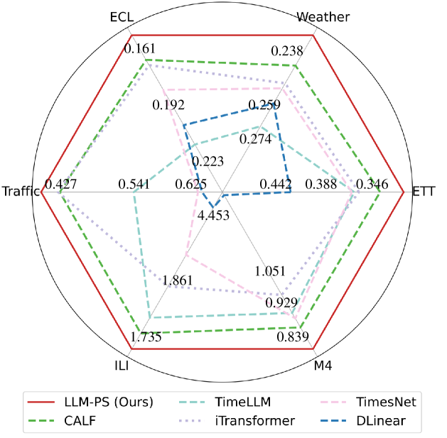
Figure 1: Performance of our proposed LLM-PS, LLM-based methods (Liu et al., 2024a; Jin et al., 2024), and conventional deep learning methods (Wu et al., 2023a; Zeng et al., 2023; Liu et al., 2024b).

1 Introduction

Time Series Forecasting (TSF) plays a crucial role in various real-world applications, such as weather forecasting (Angryk et al., 2020) and energy consumption prediction (Trindade, 2015). To achieve reliable TSF, traditional deep learning methods (Wu et al., 2023b; Zhang & Yan, 2023b; Zhou et al., 2022) usually rely on domain-specific expertise to design customized models tailored to individual tasks. However, time series data often vary significantly across different domains (Zhang et al., 2024a). For example, stock prices in the financial market frequently fluctuate in short intervals, while temperature readings from the weather station typically evolve gradually over days (Hyndman, 2018), as shown in Fig. 5. Therefore, those task-specific models struggle to generalize effectively across different applications (Jin et al., 2024). Moreover, these models are commonly trained from scratch and prone to overfitting in practical scenarios due to limited training data availability (Wen et al., 2023).

Recently, Large Language Models (LLMs), such as GPT (Brown et al., 2020) and Llama (Touvron et al., 2023), have achieved great success in natural language processing. These LLMs are pre-trained on large-scale serialized textual datasets, endowing them with strong capabilities in both contextual modeling and generalization. In general, time series and textual data share two primary similarities: 1) Sequentiality, both time series and textual data consist of ordered sets of elements; 2) Contextual dependency, the meaning of a textual sentence relies on its context, and the value at the current time point is driven by its historical data. Building on these parallels, pioneering works (Zhou et al., 2023a; Liu et al., 2024a; Jin et al., 2024; Cao et al., ) attempt to fine-tune powerful LLMs for time series generation. Among them, Liu et al. (Liu et al., 2024a) align the distributions of time series and textual data to enhance the LLM’s effectiveness in TSF. TimeLLM (Jin et al., 2024) bridges the modalities of time series and textual data by reprogramming time series data with text prototypes, thereby unlocking the TSF performance of LLMs.

Despite significant advancements in existing LLM-based methods for TSF, they generally prioritize aligning textual and time series data while ignoring the inherent characteristics of time series data, resulting in suboptimal performance. First, time series data exhibit diverse temporal patterns rarely present in textual data, including regular short-term periodic fluctuations and persistent long-term trends that evolve over time (Wu et al., 2021; Zhou et al., 2022). Second, the semantic information is spare in time series data (Cheng et al., 2023), usually requiring a prolonged period to convey specific semantics like “rapid increase” or “sudden drop”. In comparison, words in textual data generally express explicit meaning, such as “fast” or “slow”. Therefore, identifying fundamental temporal patterns and specific semantic information within time series data is crucial to guide LLMs for reliable time series prediction.

In this paper, we propose a novel LLM fine-tuning framework called LLM-PS, which enhances time series forecasting by leveraging the Patterns and Semantics in time series data. LLM-PS comprises two pivotal modules: the Multi-Scale Convolutional Neural Network (MSCNN), designed to capture the intrinsic temporal patterns, and the Time-to-Text semantic information extractor (T2T). Specifically, MSCNN extracts multi-scale features with varying receptive fields by hierarchical stacked convolutional layers. Features with small receptive fields primarily capture short-term patterns (i.e., periodicity fluctuations), while those with large receptive fields focus on long-term patterns (i.e., global trends). To further cope with short-term and long-term patterns, we decouple them from multi-scale features based on the wavelet transform and enhance them via global-to-local and local-to-global assembling. Meanwhile, T2T extracts valuable semantics by precisely predicting labels for time-series patches under a high masking ratio. Subsequently, the temporal patterns and semantics are integrated through feature transfer and input into the LLM to generate time series. Thanks to its ability to effectively handle diverse temporal patterns and accurately extract semantically rich information, LLM-PS comprehensively understands time series data, consistently achieving state-of-the-art (SOTA) performance across multiple datasets, as shown in Fig. 1.

• We recognize that time series data exhibits intrinsic characteristics that differ from those in textual data used in LLM pre-training and propose a novel TSF framework to leverage these distinctive properties to derive the LLM for reliable time series forecasting.

• We design new MSCNN and T2T modules tailored for effectively handling the diverse temporal patterns and accurately extracting semantic information, and thus enhancing the LLM’s understanding of the input time series during forecasting.

• Our LLM-PS consistently achieves SOTA performance across a variety of mainstream time series prediction tasks, especially in few-shot and zero-shot scenarios. Furthermore, our model is highly efficient while robust to noise compared with other popular methods.

2 Related Works

2.1 Time Series Forecasting

Time series forecasting aims to predict future values of a series based on historical data, serving as a crucial capability in industries like finance management (Patton, 2013), weather forecasting (Angryk et al., 2020), and energy consumption prediction (Zhou et al., 2021a). Recently, TSF methods have evolved from traditional statistical models (Taylor & Letham, 2018; Oreshkin et al., 2019a) to sophisticated deep learning models (Wu et al., 2023b; Wang et al., 2024). Deep learning methods generally utilize Recurrent Neural Networks (RNNs) (Salinas et al., 2020), Convolutional Neural Networks (CNNs) (Wu et al., 2023b), Transformers (Wu et al., 2021), and Multi-Layer Perceptrons (MLPs) (Wang et al., 2024) as their backbones. By leveraging domain expertise, they can perform well on specific tasks. Nonetheless, their real-world applicability is usually constrained by the variability of temporal patterns across domains (Jin et al., 2024).

To address these challenges, some researchers (Zhou et al., 2023a; Liu et al., 2024a) have turned to LLMs for TSF and achieved great success. Current methods primarily focus on bridging the gap between time series and textual modalities. For example, PromptCast (Xue & Salim, 2023) encodes time series and textual data into prompts to guide the LLM prediction. The prompts contain contextual information, task requirements, and the desired output format. TimeLLM (Jin et al., 2024) further enhances guidance for LLM by incorporating domain information, instructions, and data statistics within the prompts. Instead of designing prompts, (Chung et al., 2023) directly train a codebook to convert continuous time series into discrete input embeddings by mapping them to the most similar codewords in the codebook. Similarly,  (Rubenstein et al., 2023) apply K-Means clustering to time series embeddings and construct a codebook (Van Den Oord et al., 2017) by the cluster centroids. Additionally, CALF (Liu et al., 2024a) trains separate LLM branches for time series and textual data, which aligns their features across the intermediate and output layers. LLM-TS (Chen et al., 2024) employs a CNN as the time series branch and guides it with the LLM by minimizing their mutual information.

Despite the promising performance of LLM-based methods, they inadequately solve the intrinsic characteristics of time series data, limiting their effectiveness for TSF. Our LLM-PS effectively handles these properties of temporal patterns and semantics, thereby achieving reliable performance.

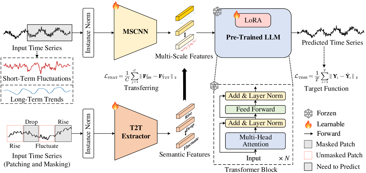
Figure 2: An overview of our proposed LLM-PS. Our LLM-PS incorporates a Multi-Scale Convolutional Neural Network (MSCNN) and Time-to-Text (T2T) semantics extractor. Specifically, for input time series $\mathbf{Y}$, MSCNN constructs multi-scale features $\mathbf{F}_{\text{MS}}$ with various receptive fields (darker colors indicate larger receptive fields), thereby capturing localized short-term fluctuations and broader long-term trends. T2T extracts features $\mathbf{F}_{\text{T2T}}$ with meaningful semantics to promote the LLM to precisely understand the input time series. Finally, the diverse temporal patterns and rich semantics are integrated via feature transferring and input into the LLM to generate precise time series $\hat{\mathbf{Y}}$.

2.2 Temporal Patterns Learning

Time series data comprises short-term fluctuations and long-term trends (Zhang & Qi, 2005). To capture these temporal patterns, existing methods (Wang et al., 2024; Kowsher et al., 2024) convert the original inputs to multiple time series inputs with varying scales through pooling operations with various window sizes. Consequently, the model can learn short-term periods and long-term trends from low-scale and high-scale inputs, respectively. However, these methods incur prohibitive computational overheads due to the intricate processing of numerous scaled signals. To address this, we introduce a new MSCNN that enables efficiently generating multi-scale features with diverse temporal patterns using a single forward, as analyzed in Section 4.4.

Besides to construct multi-scale signals, some methods (Wu et al., 2021, 2023c) directly separate temporal patterns from time series. Earlier studies (Wu et al., 2021, 2023c) employ average pooling to extract long-term trends from time series data while considering the remaining segments as short-term patterns. Recent studies (Zhou et al., 2022; Wang et al., 2024) highlighted that low-frequency and high-frequency components in the frequency domain correspond to long-term and short-term patterns, respectively. Therefore, they utilize the Fourier transform (Cochran et al., 1967) to isolate them. In this paper, we decouple short-term and long-term patterns based on the wavelet transform (Zhang, 2019). Unlike the aforementioned methods that rely on average pooling in the temporal domain or Fourier transform in the frequency domain, our method concurrently learns from both the temporal and frequency domains. Therefore, our approach can accurately decompose short-term and long-term components, as visualized in Fig. 6.

3 Approach

Time series forecasting aims to predict the series $\mathbf{Y}\in\mathbb{R}^{T\times V}$ for the next $T$ time steps given the $H$ time steps historical observations $\mathbf{X}\in\mathbb{R}^{H\times V}$, where $V$ denotes the number of variables. As shown in Fig. 2, our LLM-PS incorporates a new MSCNN (detailed in Sections 3.1&3.2) to learn multi-scale features from the input time series, which captures both short-term and long-term patterns. Meanwhile, within LLM-PS, the T2T module (described in Section 3.3) enriches the multi-scale features by the semantic information extracted from the input time series. Consequently, the multi-scale features with diverse temporal dependencies and valuable semantics are input into the LLM to facilitate accurate future time series $\hat{\mathbf{Y}}\in\mathbb{R}^{T\times V}$.

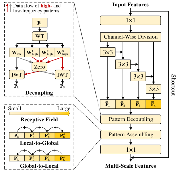
Figure 3: The diagram of our MSCNN block. The divided features are initially fed into their related 3$\times$3 convolutional layers to obtain features (e.g., $\bar{\mathbf{F}}_{1}$) with various receptive fields. Then, these features are decoupled into long-term patterns (e.g., $\mathbf{P}^{1}_{\text{L}}$) and short-term patterns (e.g., $\mathbf{P}^{1}_{\text{S}}$) using the Wavelet Transform (WT) and Inverse Wavelet Transform (IWT). Subsequently, the long-term and short-term patterns are enhanced through global-to-local and local-to-global assembling, respectively. Finally, the improved patterns are added together and passed through a 1$\times$1 convolutional layer to obtain the multi-scale features.

3.1 Multi-Scale Convolutional Neural Network

Real-world time series data is inherently complex, manifesting short-term and long-term patterns (Cleveland et al., 1990; Zhang & Qi, 2005), both of which are critical for accurate forecasting. Short-term patterns reflect localized fluctuations and periodic dynamics, while long-term patterns encapsulate broader trends that signal future trajectories. In conventional CNNs, each convolutional layer has a fixed receptive field, which limits its output features to a narrow temporal scope with only a single temporal pattern. To capture diverse temporal patterns, we follow classic CNNs (He et al., 2016; Gao et al., 2019) and design a new MSCNN stacked with bottleneck blocks. As depicted in Fig. 3, each MSCNN block learns multi-scale features by parallel branches. Features with smaller receptive fields focus on periodic fluctuations, whereas those with larger receptive fields concentrate on overarching trends.

In each MSCNN block, the $C$ channels input features $\mathbf{F}_{\text{in}}\in\mathbb{R}^{C\times V}$ first undergo 1$\times$1 convolutional layer before partitioned to $B$ branches $\{\mathbf{F}_{1},\ldots,\mathbf{F}_{B}\}$, where $\mathbf{F}_{i}\in\mathbb{R}^{C/B\times V}$ (batch dimension is omitted for simplify description). Then, $B$ branches features are recursively fed into their respective 3$\times$3 convolutional layer and added with the output of the preceding branches (except for $\mathbf{F}_{1}$), as follows:

$$\bar{\mathbf{F}}_{i}=\begin{cases}\mathbf{Conv}_{i}\left(\mathbf{F}_{i}\right),&i=1,\\ \mathbf{Conv}_{i}\left(\mathbf{F}_{i}+\bar{\mathbf{F}}_{i-1}\right),&1<i\leq B.\end{cases}$$ (1)

The receptive fields of features in $\{\bar{\mathbf{F}}_{1},\ldots,\bar{\mathbf{F}}_{B}\}$ increase sequentially as each $\bar{\mathbf{F}}_{i}$ (if $i>1$) aggregates information from preceding branches (detailed in Appendix B.3). Finally, these features are concatenated together and fused through a 1$\times$1 convolution layer to derive the output features $\mathbf{F}_{\text{out}}$:

$$\mathbf{F}_{\text{out}}=\text{Conv}_{1\times 1}(\text{Concate}(\{\bar{\mathbf{F}}_{1},\ldots,\bar{\mathbf{F}}_{B}\})+\mathbf{F}_{\text{in}},$$ (2)

where $\mathbf{F}_{\text{in}}$ is added in the output features via shortcut. Afterward, $\mathbf{F}_{\text{out}}$ is input into the subsequent MSCNN blocks to produce the multi-scale features $\mathbf{F}_{\text{MS}}$ for the LLM.

3.2 Temporal Patterns Decoupling and Assembling

In the previous section, we show how MSCNN captures diverse temporal patterns by learning multi-scale features. For a time series, its high-frequency and low-frequency components can effectively represent the corresponding short-term and long-term temporal patterns, respectively (Wang et al., 2024; Kowsher et al., 2024). Therefore, we introduce a novel patterns decoupling-assembling mechanism based on the wavelet transform (Zhang, 2019) (as shown in Fig. 3) to further refine temporal patterns in the multi-scale features.

Initially, the features $\left\{\bar{\mathbf{F}}_{1},\ldots,\bar{\mathbf{F}}_{B}\right\}$ output by $B$ branches in the MSCNN block are decoupled into low-frequency component $\mathbf{W}_{\text{low}}$ and high-frequency component $\mathbf{W}_{\text{high}}$ using the wavelet transform (see Appendix B.1) $\text{WT}(\cdot)$:

$$\mathbf{W}^{b}_{\text{low}},\{\mathbf{W}^{b}_{\text{high}\_i}\}_{i=1}^{w}\!=\!\text{WT}(\bar{\mathbf{F}}_{b},w),\quad\!\!b\in\{1,\ldots,B\}\!,$$ (3)

where $w$ denotes the decomposition levels. Subsequently, the short-term pattern $\mathbf{P}_{\text{S}}$ and long-term pattern $\mathbf{P}_{\text{L}}$ are constructed by the inverse wavelet transform $\text{IWT}(\cdot)$:

$$\left\{\begin{aligned} \mathbf{P}_{\text{S}}^{b}&=\text{IWT}(\text{Zero}(\mathbf{W}^{b}_{\text{low}}),\{\mathbf{W}^{b}_{\text{high}\_i}\}_{i=1}^{w}),\\ \mathbf{P}_{\text{L}}^{b}&=\text{IWT}(\mathbf{W}^{b}_{\text{low}},\{\text{Zero}(\mathbf{W}^{b}_{\text{high}\_i})\}_{i=1}^{w}),\end{aligned}\right.$$ (4)

where $\text{Zero}(\cdot)$ operation generates features matching the input dimensions but filled with zeros.

For features in $\left\{\bar{\mathbf{F}}_{1},\ldots,\bar{\mathbf{F}}_{B}\right\}$, their receptive fields expand sequentially. Features with smaller receptive fields more effectively capture local periodic fluctuations, whereas those with larger receptive fields focus on broader global trends. Therefore, short-/long-term patterns $\mathbf{P}_{\text{S}}$/$\mathbf{P}_{\text{L}}$ are reinforced in local-to-global/global-to-local assembling, as follows:

$$\left\{\begin{aligned} &\text{ For }b:2\rightarrow B\text{ do: }&\quad\mathbf{P}_{\text{S}}^{b}=\mathbf{P}_{\text{S}}^{b}+\mathbf{P}_{\text{S}}^{b-1},\\ &\text{ For }b:(B-1)\rightarrow 1\text{ do: }&\quad\mathbf{P}_{\text{L}}^{b}=\mathbf{P}_{\text{L}}^{b}+\mathbf{P}_{\text{L}}^{b+1}.\end{aligned}\right.$$ (5)

After the assembling, features in $\left\{\bar{\mathbf{F}}_{1},\ldots,\bar{\mathbf{F}}_{B}\right\}$ are reconstructed by combining the short-term and long-term patterns:

$$\bar{\mathbf{F}}_{b}=\mathbf{P}_{\text{S}}^{b}+\mathbf{P}_{\text{L}}^{b},\quad b\in\{1,\ldots,B\}.$$ (6)

3.3 Time-to-Text Semantics Extraction

LLMs are pre-trained on extensive textual data rich in semantic information, where individual words carry clear meaning. In comparison, time series data is semantically sparse, requiring an entire sequence to convey specific content. Consequently, LLMs pre-trained on textual data struggle to precisely interpret semantics present in time series data. Recent advancements in audio processing (Défossez et al., 2023; Zhang et al., 2024b) suggest that self-supervised learning (Devlin et al., 2018) can promote models to understand the serialized audio sequences that are similar to time series data. Inspired by them, we propose the T2T module with an encoder-decoder structure to extract semantics within time series data for the LLM, as shown in Fig. 7.

Initially, the input time series $\mathbf{X}\in\mathbb{R}^{H\times V}$ is divided into $P$ patches $\{\mathbf{X}_{i}\}^{P}_{i=1}$, where $\mathbf{X}_{i}\in\mathbb{R}^{L\times V}$ and $L$ denotes the patch length. Following (Hsu et al., 2021), approximately 75% of the patches are randomly masked. During training, the T2T module learns precise semantic information by reconstructing the masked patches while predicting their labels. The loss function is defined as:

$$\mathcal{L}_{\text{T2T}}=\frac{1}{P}\sum_{i=1}^{P}(\mathbbm{1}_{[\text{M}(i)=1]}\|\mathbf{X}_{i}-\hat{\mathbf{X}}_{i}\|_{2}+l_{i}\log\frac{l_{i}}{\hat{l_{i}}}).$$ (7)

Here, $\hat{\mathbf{X}}_{i}$ represents the reconstructed patch, $\mathbbm{1}_{[\text{M}(i)=1]}$ is the indicator function that equals 1 if the $i$-th patch is masked (i.e., $\text{M}(i)$=1); $l_{i}$ and $\hat{l}_{i}$ denote the semantic labels of the original and reconstructed patches, respectively. For a patch $\mathbf{X}_{i}$ (resp. $\hat{\mathbf{X}}_{i}$), its semantic label $l_{i}$ (resp. $\hat{l}_{i}$) is assigned as the word with the most similar LLM text embeddings, based on the similarity $\mathbf{S}_{i}$ calculated as:

$$\mathbf{S}_{i}=\text{Proj}(\mathbf{X}_{i})\cdot\mathbf{E}^{\top}.$$ (8)

Here, $\text{Proj}(\cdot)$ linearly transforms the input to the same dimensions of the LLM text embeddings $\mathbf{E}$, and “$\top$” denotes the transpose. Further details of T2T and the semantic label assignment process are provided in the Appendix B.4.

3.4 Efficient Training of LLM-PS

To efficiently train the LLM with huge parameters, we employ the parameter-efficient Low-Rank Adaptation (LoRA) (Hu et al., 2021) to fine-tune the LLM on time series data. The total objective function is defined as:

$$\mathcal{L}_{\text{OBJ}}=\mathcal{L}_{\text{TIME}}+\lambda\mathcal{L}_{\text{FEAT}},$$ (9)

where

$$\left\{\begin{aligned} &\mathcal{L}_{\text{TIME}}=\frac{1}{T}\sum_{i=1}^{T}\|\mathbf{Y}_{i}-\hat{\mathbf{Y}}_{i}\|_{2},\\ &\mathcal{L}_{\text{FEAT}}=\frac{1}{C}\sum_{j=1}^{C}\|\mathbf{F}^{j}_{\text{MS}}-\mathbf{F}^{j}_{\text{T2T}}\|_{2}.\end{aligned}\right.$$ (10)

Here, $\lambda>0$ is a trade-off parameter to balance the contributation of $\mathcal{L}_{\text{TIME}}$ and $\mathcal{L}_{\text{FEAT}}$, $\mathcal{L}_{\text{TIME}}$ encourages the LLM to forecast time series $\hat{\mathbf{Y}}$ that closely matching the ground truth $\mathbf{Y}$, $\mathcal{L}_{\text{FEAT}}$ enriches the multi-scale features $\mathbf{F}_{\text{MS}}$ through semantic alignment with the T2T-generated features $\mathbf{F}_{\text{T2T}}$.

Table 1: Average results of multivariate long-term forecasting across four different prediction lengths $T$ in the set $\{96,192,336,720\}$, and the full results are shown in Tab. 7. The best and second best results are in bold and underlined, respectively. The row “$1^{\text{st}}$ Count” records the times of each method achieving the top results. Here, we reproduce the methods with superscript “^⋆” according to their official codebase with the identical experimental setups as ours for fairness comparison. Results for other compared methods are from (Liu et al., 2024b).

Models	LLM-PS		CALF⋆		TimeLLM⋆		GPT4TS⋆		PatchTST		iTransformer		Crossformer		FEDformer		TimesNet		MICN		DLinear		TiDE
	Ours		(2024a)		(2024)		(2023b)		(2023)		(2024b)		(2023a)		(2022)		(2023a)		(2022)		(2023)		(2023)
Metric	MSE	MAE	MSE	MAE	MSE	MAE	MSE	MAE	MSE	MAE	MSE	MAE	MSE	MAE	MSE	MAE	MSE	MAE	MSE	MAE	MSE	MAE	MSE	MAE
ETTm1	0.354	0.376	0.395	0.390	0.410	0.409	0.389	0.397	0.381	0.395	0.407	0.411	0.502	0.502	0.448	0.452	0.400	0.406	0.392	0.413	0.403	0.407	0.412	0.406
ETTm2	0.262	0.314	0.281	0.321	0.296	0.340	0.285	0.331	0.285	0.327	0.291	0.335	1.216	0.707	0.305	0.349	0.291	0.333	0.328	0.382	0.350	0.401	0.289	0.326
ETTh1	0.418	0.420	0.432	0.428	0.460	0.449	0.447	0.436	0.450	0.441	0.455	0.448	0.620	0.572	0.440	0.460	0.458	0.450	0.558	0.535	0.456	0.452	0.445	0.432
ETTh2	0.350	0.390	0.349	0.382	0.389	0.408	0.381	0.408	0.366	0.394	0.381	0.405	0.942	0.684	0.437	0.449	0.414	0.427	0.587	0.525	0.559	0.515	0.611	0.550
Weather	0.238	0.269	0.250	0.274	0.274	0.290	0.264	0.284	0.258	0.280	0.257	0.279	0.259	0.315	0.309	0.360	0.259	0.287	0.242	0.299	0.265	0.317	0.271	0.320
Electricity	0.161	0.254	0.175	0.265	0.223	0.309	0.205	0.290	0.216	0.304	0.178	0.270	0.244	0.334	0.214	0.327	0.192	0.295	0.186	0.294	0.212	0.300	0.251	0.344
Traffic	0.427	0.279	0.439	0.281	0.541	0.358	0.488	0.317	0.555	0.361	0.428	0.282	0.550	0.304	0.610	0.376	0.620	0.336	0.541	0.315	0.625	0.383	0.760	0.473
ILI	1.735	0.854	1.861	0.924	1.829	0.924	1.871	0.852	2.145	0.897	2.258	0.957	3.749	1.284	2.705	1.097	2.267	0.927	2.985	1.186	4.453	1.553	5.216	1.614
ECG	0.225	0.250	0.258	0.260	0.250	0.264	0.262	0.260	0.253	0.277	0.257	0.271	0.244	0.269	0.255	0.279	0.291	0.305	0.305	0.314	0.291	0.307	0.291	0.307
$1^{\text{st}}$ Count	15		2		0		1		0		0		0		0		0		0		0		0

Table 2: Results of short-term forecasting across monthly, quarterly, yearly, and others subsets. The input and output time series lengths are $[12,96]$ and $[6,48]$, respectively.

Models		LLM-PS	CALF	TimeLLM	GPT4TS	PatchTST	iTransformer	ETSformer	FEDformer	Autoformer	TimesNet	TCN	N-HiTS	N-BEATS	DLinear	LSSL	LSTM
		(Ours)	(2024a)	(2024)	(2023b)	(2023)	(2024b)	(2022)	(2022)	(2021)	(2023a)	(2018)	(2022)	(2019b)	(2023)	(2022)	(1997)
Yearly	SMAPE	13.277	13.314	13.419	13.531	13.477	14.252	18.009	13.728	13.974	13.387	14.920	13.418	13.436	16.965	16.675	176.040
	MASE	2.973	3.009	3.005	3.015	3.019	3.208	4.487	3.048	3.134	2.996	3.364	3.045	3.043	4.283	19.953	31.033
	OWA	0.780	0.786	0.789	0.793	0.792	0.840	1.115	0.803	0.822	0.786	0.880	0.793	0.794	1.058	4.397	9.290
Quarterly	SMAPE	9.995	10.049	10.110	10.177	10.380	10.755	13.376	10.792	11.338	10.100	11.122	10.202	10.124	12.145	65.999	172.808
	MASE	1.164	1.166	1.178	1.194	1.233	1.284	1.906	1.283	1.365	1.182	1.360	1.194	1.169	1.520	17.662	19.753
	OWA	0.878	0.871	0.889	0.898	0.921	0.957	1.302	0.958	1.012	0.890	1.001	0.899	0.886	1.106	9.436	15.049
Monthly	SMAPE	12.585	12.624	12.980	12.894	12.959	13.721	14.588	14.260	13.958	12.679	15.626	12.791	12.677	13.514	64.664	143.237
	MASE	0.924	0.922	0.963	0.956	0.970	1.074	1.368	1.102	1.103	0.933	1.274	0.969	0.937	1.037	16.245	16.551
	OWA	0.871	0.871	0.903	0.897	0.905	0.981	1.149	1.012	1.002	0.878	1.141	0.899	0.880	0.956	9.879	12.747
Others	SMAPE	4.550	4.773	4.795	4.940	4.952	5.615	7.267	4.954	5.485	4.891	7.186	5.061	4.925	6.709	121.844	186.282
	MASE	3.089	3.119	3.178	3.228	3.347	3.977	5.240	3.264	3.865	3.302	4.677	3.216	3.391	4.953	91.650	119.294
	OWA	0.966	0.990	1.006	1.029	1.049	1.218	1.591	1.036	1.187	1.035	1.494	1.040	1.053	1.487	27.273	38.411
Average	SMAPE	11.721	11.770	11.983	11.991	12.059	12.726	14.718	12.840	12.909	11.829	13.961	11.927	11.851	13.639	67.156	160.031
	MASE	1.561	1.570	1.595	1.600	1.623	15.336	2.408	1.701	1.771	1.585	1.945	1.613	1.599	2.095	21.208	25.788
	OWA	0.840	0.845	0.859	0.861	0.869	0.929	1.172	0.918	0.939	0.851	1.023	0.861	0.855	1.051	8.021	12.642
$1^{\text{st}}$ Count		14	2	0	0	0	0	0	0	0	0	0	0	0	0	0	0

4 Experiments

To demonstrate the effectiveness of our proposed LLM-PS, we conduct intensive experiments on multiple widely used time series datasets for various tasks, including long-term, short-term, few-shot, and zero-shot forecasting.
Baselines. We compare our LLM-PS with a large range of SOTA methods, mainly including: 1) LLM-based methods: CALF (2024a), GPT4TS (2023b), and TimeLLM (2024); 2) Transformer-based methods: Crossformer (2023a), FEDformer (2022), PatchTST (2023), iTransformer (2024b), ETSformer (2022), and Autoformer (2021); 3) CNN-based methods: TimesNet (2023a), TCN (2018), and MICN (2022); 4) MLP-based methods: DLinear (2023), TiDE (2023), and TimeMixer (2024). Besides, classical works N-HiTS (2022) and N-BEATS (2019b) are also included for short-term forecasting. The details of these comparison methods can be found in the Appendix A.1.
Implementation Details. We follow (Zhou et al., 2023b; Liu et al., 2024a) and employ the pre-trained GPT2 model (Radford et al., 2019) (the first six layers) as the default LLM backbone. Our LLM-PS utilizes Adam as the optimizier and the learning rate is 0.0005. For the parameter-efficient LoRA, its rank, scale factor, and dropout ratio are set to 8, 32, and 0.1, respectively. Additionally, the trade-off parameter $\lambda$ in Eq. (9) is set to 0.01 and its parametric sensitivities are analyzed in Appendix B.5.

Table 3: Average results of few-shot forecasting with 10% training data, where the prediction lengths $T\in\{96,192,336,720\}$ and the full results are provided in Tab. 8.

Models	LLM-PS		CALF		TimeLLM		GPT4TS		PatchTST		Crossformer		FEDformer		TimesNet		MICN		DLinear		TiDE
	Ours		(2024a)		(2024)		(2023b)		(2023)		(2023a)		(2022)		(2023a)		(2022)		(2023)		(2023)
Metric	MSE	MAE	MSE	MAE	MSE	MAE	MSE	MAE	MSE	MAE	MSE	MAE	MSE	MAE	MSE	MAE	MSE	MAE	MSE	MAE	MSE	MAE
ETTm1	0.497	0.454	0.504	0.462	0.636	0.512	0.608	0.500	0.557	0.483	1.340	0.848	0.696	0.572	0.673	0.534	0.970	0.674	0.567	0.499	0.515	0.469
ETTm2	0.281	0.324	0.302	0.330	0.348	0.343	0.303	0.336	0.295	0.334	1.985	1.048	0.356	0.392	0.321	0.354	1.073	0.716	0.329	0.382	0.303	0.337
ETTh1	0.632	0.546	0.644	0.541	0.765	0.584	0.689	0.555	0.683	0.546	1.744	0.914	0.750	0.607	0.865	0.625	1.405	0.814	0.647	0.552	0.779	0.604
ETTh2	0.409	0.420	0.419	0.427	0.589	0.498	0.579	0.497	0.550	0.487	3.139	1.378	0.553	0.525	0.476	0.463	2.533	1.158	0.441	0.458	0.421	0.428
$1^{\text{st}}$ Count	7		1		0		0		0		0		0		0		0		0		0

Table 4: Average results of zero-shot forecasting, where prediction lengths $T\in\{96,192,336,720\}$ and Tab. 9 shows the full results. The term “ETTh1 $\to$ ETTm1” indicates that models trained on the ETTh1 dataset and are evaluated on the ETTm1 dataset, the convention is also followed for other terms.

Models	LLM-PS		CALF		TimeLLM		GPT4TS		PatchTST		Crossformer		FEDformer		TimesNet		MICN		DLinear		TiDE
	Ours		(2024a)		(2024)		(2023b)		(2023)		(2023a)		(2022)		(2023a)		(2022)		(2023)		(2023)
Metric	MSE	MAE	MSE	MAE	MSE	MAE	MSE	MAE	MSE	MAE	MSE	MAE	MSE	MAE	MSE	MAE	MSE	MAE	MSE	MAE	MSE	MAE
ETTh1 $\rightarrow$ ETTm1	0.721	0.541	0.755	0.574	0.847	0.565	0.798	0.574	0.894	0.610	0.999	0.736	0.765	0.588	0.794	0.575	1.439	0.780	0.760	0.577	0.774	0.574
ETTh1 $\rightarrow$ ETTm2	0.316	0.361	0.316	0.355	0.315	0.357	0.317	0.359	0.318	0.362	1.120	0.789	0.357	0.403	0.339	0.370	2.428	1.236	0.399	0.439	0.314	0.355
ETTh2 $\rightarrow$ ETTm1	0.714	0.552	0.836	0.586	0.868	0.595	0.920	0.610	0.871	0.596	1.195	0.711	0.741	0.588	1.286	0.705	0.764	0.601	0.778	0.594	0.841	0.590
ETTh2 $\rightarrow$ ETTm2	0.322	0.359	0.319	0.360	0.322	0.363	0.331	0.371	0.420	0.433	2.043	1.124	0.365	0.405	0.361	0.390	0.527	0.519	0.496	0.496	0.321	0.364
$1^{\text{st}}$ Count	5		2		0		0		0		0		0		0		0		0		2

4.1 Long-Term Forecasting

Setups. We conduct intensive experiments across various popular real-world datasets, including four Electricity Transformer Temperature (ETT) subsets (ETTh1, ETTh2, ETTm1, and ETTm2) (Zhou et al., 2021a), Weather, Electricity, Traffic, Illness (Wu et al., 2021), and Electrocardiography (ECG) (Moody & Mark, 2001) datasets. The input length $H$ of time series data is set to 96, with prediction lengths $T$ spanning $\{96,192,336,720\}$. The evaluation metrics are Mean Squared Error (MSE) and Mean Absolute Error (MAE), where lower values of these metrics indicate better model performance. The dataset descriptions are provided in Appendix A.2.
Results. Tab. 1 reports the brief average results of long-term forecasting with various prediction lengths. Firstly, we can observe that our LLM-PS surpasses the baseline methods in most instances, achieving the top results in 15 of 18 cases. Secondly, compared with the SOTA LLM-based methods, i.e., CALF, TimeLLM, and GPT4TS, our approach achieves consistent MSE/MAE reductions of 6%/3%, 11%/9%, and 9%/5%, respectively. Thirdly, our method significantly outperforms traditional deep learning methods based on Transformer, CNN, and MLP, especially on the Traffic, ILI, and ECG datasets. These results indicate that our LLM-PS can precisely predict long-term time series by effectively leveraging temporal patterns and semantics within the input series with limited length.

4.2 Short-Term Forecasting

Setups. We evaluate the M4 dataset (Makridakis et al., 2018), which records marketing data in monthly, quarterly, yearly, and others. For short-term forecasting, the prediction horizons are relatively small and range in $[6,48]$, while the input lengths are twice their corresponding prediction horizons. The evaluation metrics are Mean Absolute Scaled Error (MSAE), Symmetric Mean Absolute Percentage Error (SMAPE), and Overall Weighted Average (OWA). Formal definitions of these metrics are provided in Appendix A.3.
Results. The results of short-term forecasting across monthly, quarterly, yearly, and others subsets are shown in Tab. 2. Our proposed LLM-PS achieves a SMAPE of 11.721, a MASE of 1.561, and an OWA of 0.840, which consistently outperforms other compared methods.

4.3 Few/Zero-Shot Forecasting

Setups. LLMs possess powerful few-shot and zero-shot learning capabilities (Zhou et al., 2023b; Jin et al., 2024), which are crucial for time series forecasting in real-world scenarios. We also verify the few-shot and zero-shot learning performance of our LLM-PS. For few-shot forecasting, there are only 10% training data of ETT datasets are available. For zero-shot forecasting, LLMs trained on one dataset are directly tested on other datasets. The training setups are the same as those in long-term forecasting.
Results. The average results over various prediction horizons for the challenging few-shot forecasting tasks are reported in Tab. 3. In such cases, our LLM-PS always achieves the best results in 7 of 8 cases, which demonstrates that our LLM-PS can effectively learn valuable temporal information only using limited data. Compared with the LLM-based methods, i.e., CALF, TimeLLM, and GPT4TS, our method yields 3%, 17%, and 13% performance improvements, respectively.

In addition to the few-shot learning tasks, we also considered the more challenging zero-shot learning tasks. The experimental results are provided in Tab. 4. Our method significantly outperforms the comparison methods in 5 of 8 cases. Notably, our LLM-PS outperforms CALF, TimeLLM, and GPT4TS, which also fine-tune the LLM for time series forecasting, showing performance improvements of 5%, 8%, and 9%, respectively.

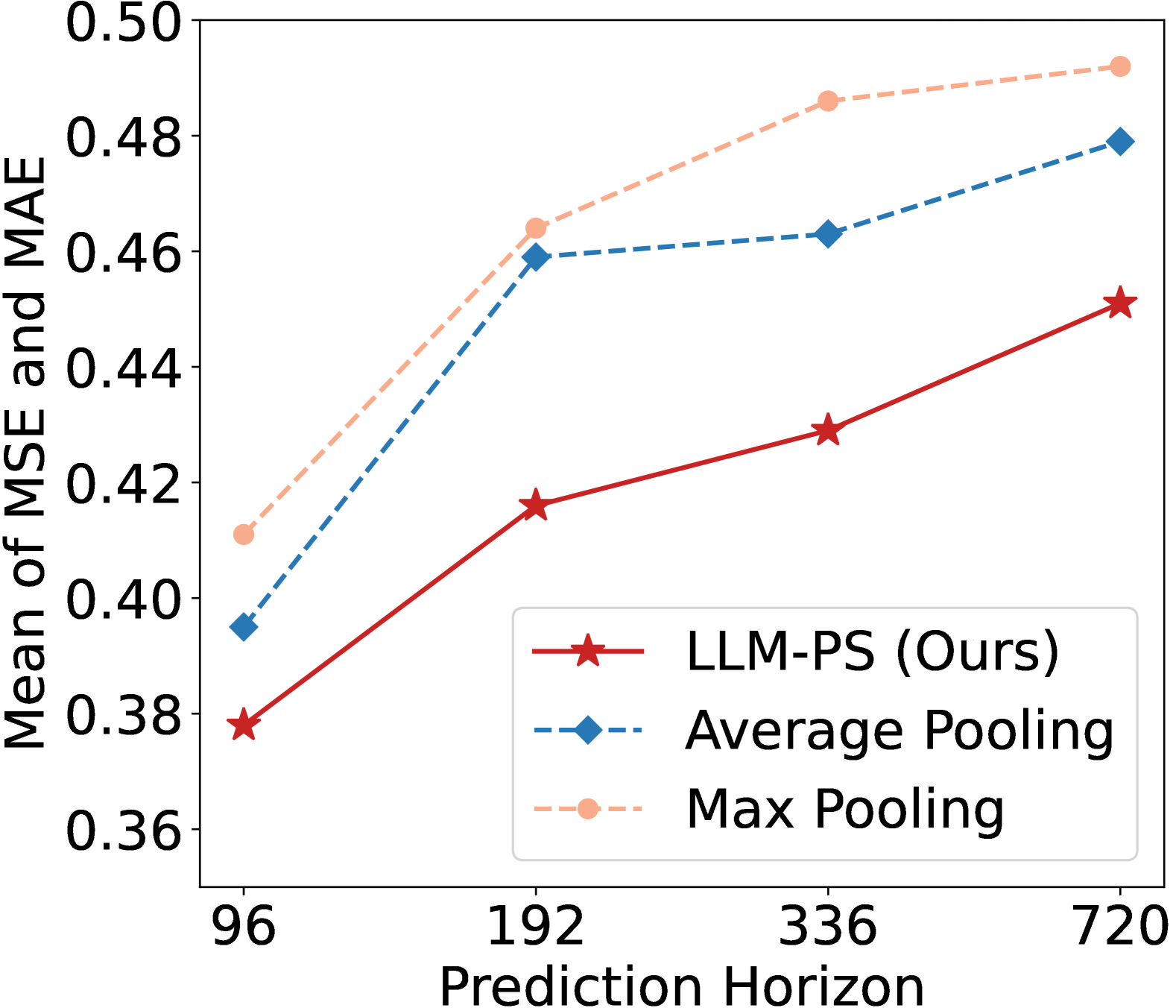
(a)

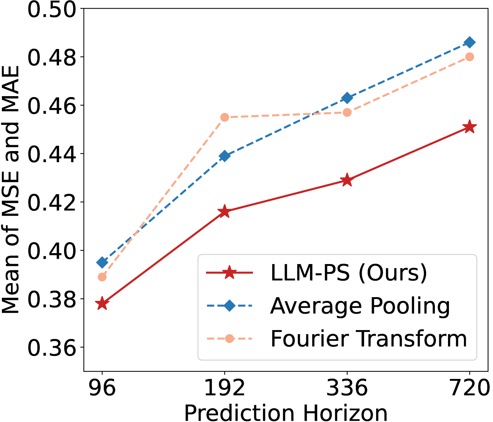
(b)

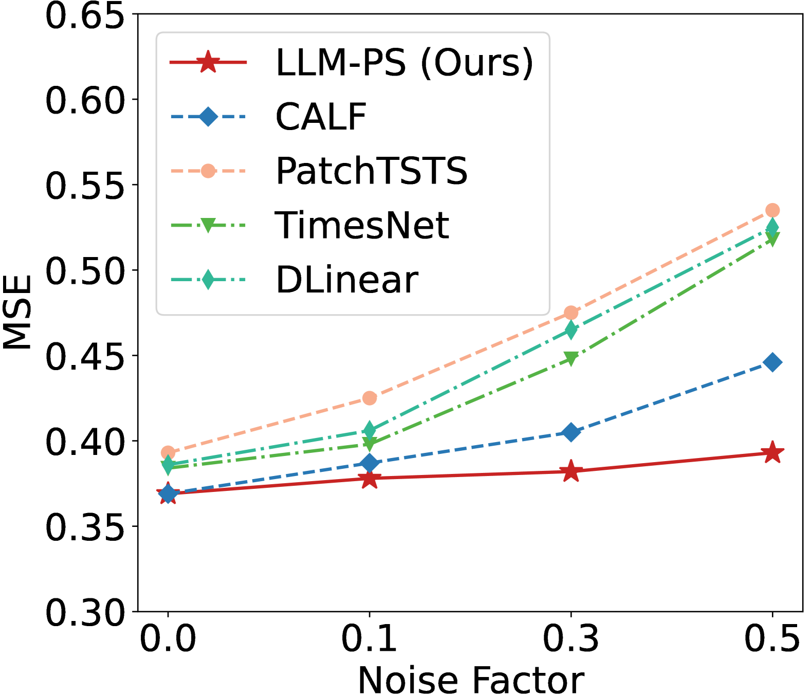
(c)

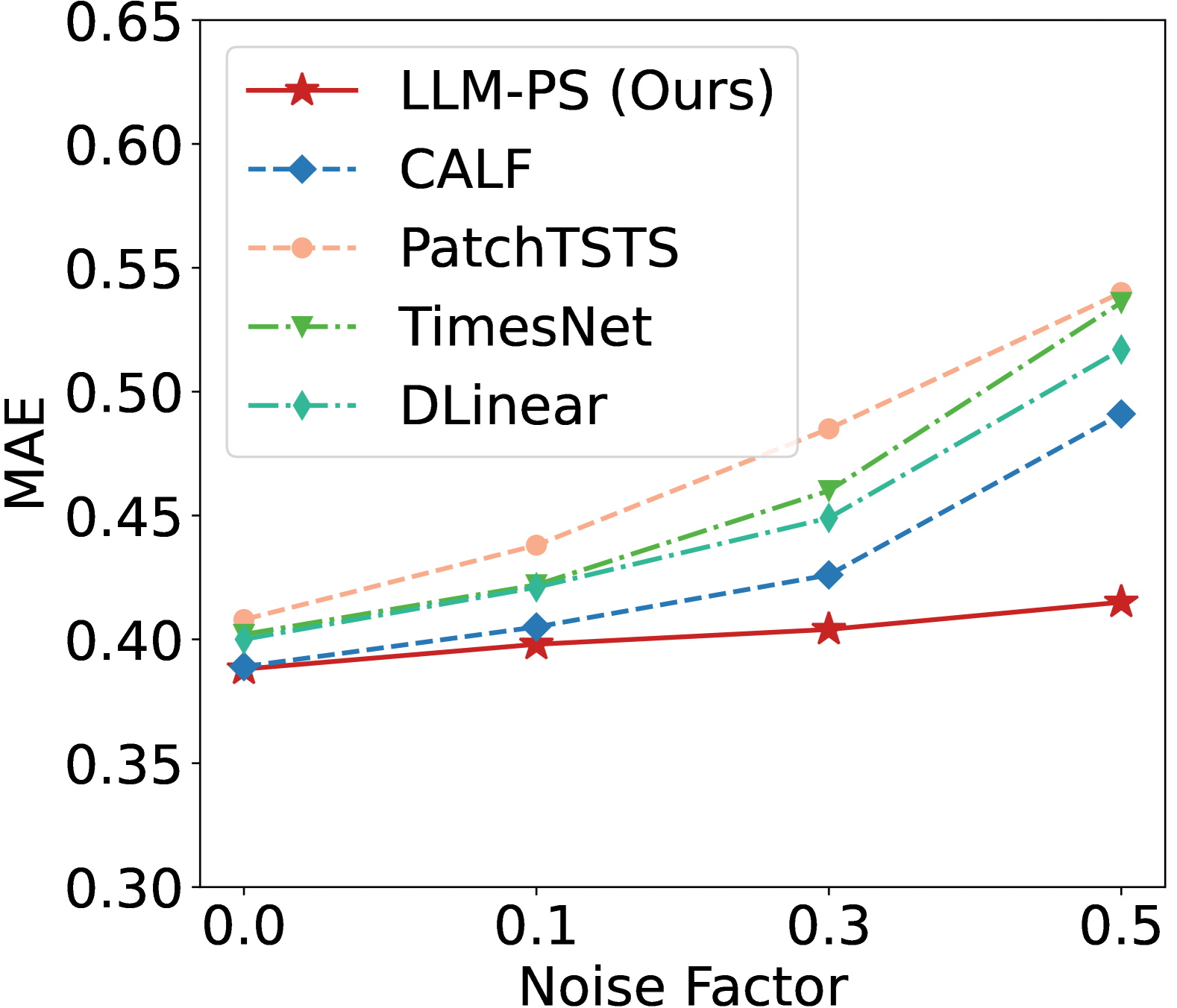
(d)

Figure 4: Analysis of (a) multi-scale feature extraction and (b) temporal patterns decoupling. Subfigures (c) and (d) show the MSE/MAE of various methods on noisy ETTh1 datasets. Notably, lower MSE/MAE indicates better model performance.

4.4 Model Analysis

Multi-Scale Feature Extraction. We compare our MSCNN against existing multi-scale features extraction techniques (Kowsher et al., 2024), which convert the input time series into diverse scales using average or max pooling layers with varying window sizes. As shown in Fig. 4(a), our method consistently outperforms those employing pooling operations. These results indicate that our method excels in extracting the multi-scale features, thereby effectively capturing the short-term and long-term patterns in input time series. Further analysis is provided in Appendix B.2.
Temporal Patterns Decoupling. We compare our wavelet-transform-based decoupling with the Fourier-transform-based and pooling-based decoupling techniques used in existing methods (Wu et al., 2021; Wang et al., 2024). As shown in Fig. 4(b), our decoupling operation based on wavelet transform achieves better performance than those based on Fourier transform and average pooling. The short-term and long-term components decomposed by our LLM-PS and compared methods are visualized in Fig. 6.
Semantic Information Utilization. Tab. 5 reports the results of ablating our proposed T2T module for semantic information learning. It can be found that the performance of LLM decreases in 9 of 10 cases, which demonstrates that the semantic information extracted by our T2T is helpful in enhancing the TSF performance of LLM. The detailed structure of the T2T module is provided in Appendix B.4.

Table 5: Long-term forecasting results of ablating our proposed T2T module on the ETTh1 dataset.

Type	MSE / MAE
	96	192	336	720	Mean
w/o T2T	0.373 / 0.395	0.416 / 0.425	0.439 / 0.432	0.464 /0.470	0.426 /0.431
LLM-PS	0.369 / 0.388	0.418 / 0.415	0.432 / 0.426	0.452 / 0.451	0.418 / 0.420

Model Efficiency. We evaluate the efficiency of our method with other LLM fine-tuning methods on four datasets, including ETTh1, ETTm1, Weather, and Traffic. For a fair comparison, all experiments adopt the same experimental settings and LLM backbone (i.e., GPT2), where input length, prediction length, and patience for early stopping are set to 96, 96, and 5, respectively. All experiments are conducted on a single NVIDIA RTX 4090 GPU. As reported in Tab. 6, our proposed LLM-PS achieves the best performance with significantly lower training costs. Compared with LLMMixer, which also learns multi-scale features from the multiple input series with various scales, our method attains a 17% performance edge while utilizing just 9% of the training time. These experimental results indicate that our method can efficiently and effectively learn the temporal patterns and semantic information from time series data, and thus achieving reliable TSF performance.

Table 6: The fine-tuning costs, mean MSE/MAE across four datasets of our LLM-PS and other LLM-based methods.

Model	Time (s)				Mean MSE	Mean MAE
	ETTh1	ETTm1	Weather	Traffic
GPT4TS (2023b)	421	1140	4565	59164	0.339	0.323
Time-LLM (2024)	2780	11929	36188	465136	0.372	0.346
LLMMixer (2024)	635	2493	9640	10464	0.372	0.346
CALF (2024a)	354	1394	1259	4929	0.315	0.302
LLM-PS (Ours)	192	481	260	1092	0.301	0.298

Noisy Data. Time series data in real-world applications is usually noisy due to measurement errors and missing values. In such cases, the target time series is more challenging than that in training data, and the models are hard to predict reliably. To assess the robustness of our LLM-PS against noise, we evaluate it on the ETTh1 dataset with Gaussian noise, where the noise factors are in $[0.0,0.1,0.3,0.5]$. Both the input and prediction lengths are set to 96. As reported in Fig. 4(c)&4(d), our method consistently achieves superior performance across various noise factors. In particular, our method outperforms other comparison approaches by an even more significant margin as the noise factor increases. These experimental results demonstrate that our LLM-PS is robust to noise and can be effectively applied to real-world scenarios for time series forecasting.

5 Conclusion

In this paper, we identify the intrinsic characteristics of time series data, i.e., diverse temporal patterns and semantic sparsity. These properties are critical for reliable time series forecasting but are usually neglected by existing LLM-based methods, and thus resulting in suboptimal performance. To address this problem, we propose LLM-PS, a novel TSF framework that learns fundamental temporal patterns and valuable semantics from time series data through the novel MSCNN and T2T modules. As a result, our LLM-PS can comprehensively understand time series data, thereby enabling accurate generation of time series. Our intensive experiments demonstrate that LLM-PS achieves SOTA performance across multiple benchmark datasets spanning critical real-world domains, mainly including finance, energy, transportation, and healthcare.

Impact Statement

This paper proposes a novel framework, LLM-PS, which aims to advance time series forecasting using large language models. Our work focuses on integrating temporal patterns and semantics in time series data, enabling state-of-the-art performance in various forecasting scenarios.

We anticipate several potential societal benefits, including improved decision-making in critical areas such as finance, healthcare, and energy management. However, as with any machine learning advancement, ethical considerations must be acknowledged, including the potential misuse of forecasting technologies in domains like financial speculation or surveillance. To mitigate these risks, we encourage responsible and transparent applications of our methods.

In conclusion, we do not identify any immediate ethical concerns or risks unique to our methodology, and we believe it can benefit society.

Appendix A Full Experimental Results

Table 7: Full results for long-term forecasting consider prediction horizons $H$ within $\{96,192,336,720\}$. The term “Avg.” represents the average results across the four prediction lengths. The best and second best outcomes are highlighted in bold and underlined, respectively. The notation “$1^{\text{st}}$ Count” denotes the frequency of each method achieving the top results.

Categories		LLM-based								Transformer-based												CNN-based				MLP-based
Models		LLM-PS		CALF		TimeLLM		GPT4TS		PatchTST		iTransformer		Crossformer		FEDformer		Autoformer		Informer		TimesNet		MICN		DLinear		TiDE
		Ours		((2024a))		(2024)		(2023b)		(2023)		(2024b)		(2023a)		(2022)		(2021)		(2021b)		(2023a)		(2022)		(2023)		(2023)
Metric		MSE	MAE	MSE	MAE	MSE	MAE	MSE	MAE	MSE	MAE	MSE	MAE	MSE	MAE	MSE	MAE	MSE	MAE	MSE	MAE	MSE	MAE	MSE	MAE	MSE	MAE	MSE	MAE
ETTm1	96	0.288	0.334	0.323	0.349	0.359	0.381	0.329	0.364	0.321	0.360	0.341	0.376	0.360	0.401	0.379	0.419	0.505	0.475	0.672	0.571	0.338	0.375	0.316	0.362	0.345	0.372	0.352	0.373
	192	0.333	0.361	0.374	0.375	0.383	0.393	0.368	0.382	0.362	0.384	0.382	0.395	0.402	0.440	0.426	0.441	0.553	0.496	0.795	0.669	0.374	0.387	0.363	0.390	0.380	0.389	0.389	0.391
	336	0.367	0.386	0.409	0.399	0.416	0.414	0.400	0.403	0.392	0.402	0.418	0.418	0.543	0.528	0.445	0.459	0.621	0.537	1.212	0.871	0.410	0.411	0.408	0.426	0.413	0.413	0.423	0.413
	720	0.429	0.424	0.477	0.438	0.483	0.449	0.460	0.439	0.450	0.435	0.487	0.456	0.704	0.642	0.543	0.490	0.671	0.561	1.166	0.823	0.478	0.450	0.481	0.476	0.474	0.453	0.485	0.448
	Avg.	0.354	0.376	0.395	0.390	0.410	0.409	0.389	0.397	0.381	0.395	0.407	0.411	0.502	0.502	0.448	0.452	0.588	0.517	0.961	0.734	0.400	0.406	0.392	0.413	0.403	0.407	0.412	0.406
ETTm2	96	0.170	0.254	0.178	0.256	0.193	0.280	0.178	0.263	0.178	0.260	0.185	0.272	0.273	0.356	0.203	0.287	0.255	0.339	0.365	0.453	0.187	0.267	0.179	0.275	0.193	0.292	0.181	0.264
	192	0.224	0.289	0.242	0.297	0.257	0.318	0.245	0.306	0.249	0.307	0.253	0.313	0.426	0.487	0.269	0.328	0.249	0.309	0.281	0.340	0.533	0.563	0.307	0.376	0.284	0.362	0.246	0.304
	336	0.280	0.327	0.307	0.339	0.317	0.353	0.309	0.347	0.313	0.346	0.315	0.350	1.013	0.714	0.325	0.366	0.339	0.372	1.363	0.887	0.321	0.351	0.325	0.388	0.369	0.427	0.307	0.341
	720	0.374	0.384	0.397	0.393	0.419	0.411	0.409	0.408	0.400	0.398	0.413	0.406	3.154	1.274	0.421	0.415	0.433	0.432	3.379	1.338	0.408	0.403	0.502	0.490	0.554	0.522	0.407	0.397
	Avg.	0.262	0.314	0.281	0.321	0.296	0.340	0.285	0.331	0.285	0.327	0.291	0.335	1.216	0.707	0.305	0.349	0.327	0.371	1.410	0.810	0.291	0.333	0.328	0.382	0.350	0.401	0.289	0.326
ETTh1	96	0.369	0.388	0.369	0.389	0.398	0.410	0.376	0.397	0.393	0.408	0.386	0.404	0.420	0.439	0.376	0.419	0.449	0.459	0.865	0.713	0.384	0.402	0.421	0.431	0.386	0.400	0.384	0.393
	192	0.418	0.415	0.427	0.423	0.451	0.440	0.438	0.426	0.445	0.434	0.441	0.436	0.540	0.519	0.420	0.448	0.436	0.429	0.500	0.482	1.008	0.792	0.474	0.487	0.437	0.432	0.436	0.422
	336	0.432	0.426	0.456	0.436	0.508	0.471	0.479	0.446	0.484	0.451	0.489	0.461	0.722	0.648	0.459	0.465	0.521	0.496	1.107	0.809	0.491	0.469	0.569	0.551	0.481	0.459	0.480	0.445
	720	0.452	0.451	0.479	0.467	0.483	0.478	0.495	0.476	0.480	0.471	0.508	0.493	0.799	0.685	0.506	0.507	0.514	0.512	1.181	0.865	0.521	0.500	0.770	0.672	0.519	0.516	0.481	0.469
	Avg.	0.418	0.420	0.432	0.428	0.460	0.449	0.447	0.436	0.450	0.441	0.455	0.448	0.620	0.572	0.440	0.460	0.496	0.487	1.040	0.795	0.458	0.450	0.558	0.535	0.456	0.452	0.445	0.432
ETTh2	96	0.279	0.341	0.279	0.331	0.295	0.346	0.295	0.348	0.294	0.343	0.300	0.349	0.745	0.584	0.358	0.397	0.346	0.388	3.755	1.525	0.340	0.374	0.299	0.364	0.333	0.387	0.400	0.440
	192	0.356	0.387	0.353	0.380	0.386	0.399	0.386	0.404	0.377	0.393	0.379	0.398	0.877	0.656	0.429	0.439	0.456	0.452	5.602	1.931	0.402	0.414	0.441	0.454	0.477	0.476	0.528	0.509
	336	0.350	0.393	0.362	0.394	0.447	0.443	0.421	0.435	0.381	0.409	0.418	0.429	1.043	0.731	0.496	0.487	0.482	0.486	4.721	1.835	0.452	0.452	0.654	0.567	0.594	0.541	0.643	0.571
	720	0.413	0.437	0.404	0.426	0.428	0.444	0.422	0.445	0.412	0.433	0.428	0.445	1.104	0.763	0.463	0.474	0.515	0.511	3.647	1.625	0.462	0.468	0.956	0.716	0.831	0.657	0.874	0.679
	Avg.	0.350	0.390	0.349	0.382	0.389	0.408	0.381	0.408	0.366	0.394	0.381	0.405	0.942	0.684	0.437	0.449	0.450	0.459	4.431	1.729	0.414	0.427	0.587	0.525	0.559	0.515	0.611	0.550
Weather	96	0.157	0.205	0.164	0.204	0.195	0.233	0.182	0.223	0.177	0.218	0.174	0.214	0.158	0.230	0.217	0.296	0.266	0.336	0.300	0.384	0.172	0.220	0.161	0.229	0.196	0.255	0.202	0.261
	192	0.202	0.245	0.214	0.250	0.240	0.269	0.231	0.263	0.225	0.259	0.221	0.254	0.206	0.277	0.276	0.336	0.307	0.367	0.598	0.544	0.219	0.261	0.220	0.281	0.237	0.296	0.242	0.298
	336	0.255	0.286	0.269	0.291	0.293	0.306	0.283	0.300	0.278	0.297	0.278	0.296	0.272	0.335	0.339	0.380	0.359	0.395	0.578	0.523	0.280	0.306	0.278	0.331	0.283	0.335	0.287	0.335
	720	0.336	0.338	0.355	0.352	0.368	0.354	0.360	0.350	0.354	0.348	0.358	0.349	0.398	0.418	0.403	0.428	0.419	0.428	1.059	0.741	0.365	0.359	0.311	0.356	0.345	0.381	0.351	0.386
	Avg.	0.238	0.269	0.250	0.274	0.274	0.290	0.264	0.284	0.258	0.280	0.257	0.279	0.259	0.315	0.309	0.360	0.338	0.382	0.634	0.548	0.259	0.287	0.242	0.299	0.265	0.317	0.271	0.320
Electricity	96	0.131	0.222	0.145	0.238	0.204	0.293	0.185	0.272	0.195	0.285	0.148	0.240	0.219	0.314	0.193	0.308	0.201	0.317	0.274	0.368	0.168	0.272	0.164	0.269	0.197	0.282	0.237	0.329
	192	0.151	0.240	0.161	0.252	0.207	0.295	0.189	0.276	0.199	0.289	0.162	0.253	0.231	0.322	0.201	0.315	0.222	0.334	0.296	0.386	0.184	0.289	0.177	0.285	0.196	0.285	0.236	0.330
	336	0.162	0.256	0.175	0.267	0.219	0.308	0.204	0.291	0.215	0.305	0.178	0.269	0.246	0.337	0.214	0.329	0.231	0.338	0.300	0.394	0.198	0.300	0.193	0.304	0.209	0.301	0.249	0.344
	720	0.213	0.297	0.222	0.303	0.263	0.341	0.245	0.324	0.256	0.337	0.225	0.317	0.280	0.363	0.246	0.355	0.254	0.361	0.373	0.439	0.220	0.320	0.212	0.321	0.245	0.333	0.284	0.373
	Avg.	0.164	0.254	0.175	0.265	0.223	0.309	0.205	0.290	0.216	0.304	0.178	0.270	0.244	0.334	0.214	0.327	0.227	0.338	0.311	0.397	0.192	0.295	0.186	0.294	0.212	0.300	0.251	0.344
Traffic	96	0.392	0.267	0.407	0.268	0.536	0.359	0.468	0.307	0.544	0.359	0.395	0.268	0.522	0.290	0.587	0.366	0.613	0.388	0.719	0.391	0.593	0.321	0.519	0.309	0.650	0.396	0.805	0.493
	192	0.413	0.265	0.430	0.278	0.530	0.354	0.476	0.311	0.540	0.354	0.417	0.276	0.530	0.293	0.604	0.373	0.616	0.382	0.696	0.379	0.617	0.336	0.537	0.315	0.598	0.370	0.756	0.474
	336	0.440	0.282	0.444	0.281	0.530	0.349	0.488	0.317	0.551	0.358	0.433	0.283	0.558	0.305	0.621	0.383	0.622	0.337	0.777	0.420	0.629	0.336	0.534	0.313	0.605	0.373	0.762	0.477
	720	0.464	0.300	0.477	0.300	0.569	0.371	0.521	0.333	0.586	0.375	0.467	0.302	0.589	0.328	0.626	0.382	0.660	0.408	0.864	0.472	0.640	0.350	0.577	0.325	0.645	0.394	0.719	0.449
	Avg.	0.427	0.279	0.439	0.281	0.541	0.358	0.488	0.317	0.555	0.361	0.428	0.282	0.550	0.304	0.610	0.376	0.628	0.379	0.764	0.416	0.620	0.336	0.541	0.315	0.625	0.383	0.760	0.473
ILI	24	1.630	0.798	1.672	0.841	1.651	0.841	1.869	0.823	2.221	0.883	2.321	0.937	3.449	1.238	2.721	1.133	3.280	1.265	5.280	1.578	1.826	0.893	2.715	1.125	5.060	1.709	5.855	1.633
	36	1.650	0.821	1.725	0.872	1.701	0.861	1.853	0.854	2.313	0.904	2.188	0.945	3.743	1.271	2.768	1.118	3.424	1.271	5.094	1.565	2.678	0.986	2.817	1.154	4.413	1.549	5.598	1.715
	48	1.810	0.921	1.937	0.937	2.153	1.041	1.886	0.855	2.048	0.886	2.231	0.956	3.853	1.306	2.637	1.088	3.009	1.520	4.884	1.530	2.584	0.937	3.038	1.199	4.109	1.473	4.795	1.568
	60	1.850	0.874	2.128	0.999	2.064	0.953	1.877	0.877	2.008	0.915	2.292	0.991	3.951	1.323	2.696	1.050	2.803	1.133	5.326	1.571	1.980	0.894	3.372	1.269	4.233	1.481	4.616	1.543
	Avg.	1.735	0.854	1.861	0.924	1.829	0.924	1.871	0.852	2.145	0.897	2.258	0.957	3.749	1.284	2.705	1.097	3.129	1.297	5.123	1.561	2.267	0.927	2.985	1.186	4.453	1.553	5.216	1.614
ECG	96	0.122	0.173	0.185	0.175	0.143	0.179	0.212	0.198	0.159	0.195	0.210	0.212	0.143	0.194	0.214	0.223	0.163	0.183	0.201	0.238	0.261	0.270	0.276	0.264	0.264	0.270	0.255	0.256
	192	0.196	0.223	0.235	0.234	0.234	0.245	0.241	0.236	0.237	0.259	0.244	0.255	0.214	0.246	0.237	0.263	0.217	0.237	0.246	0.243	0.283	0.293	0.292	0.306	0.279	0.295	0.273	0.291
	336	0.261	0.277	0.286	0.290	0.288	0.287	0.267	0.270	0.278	0.301	0.267	0.286	0.284	0.286	0.261	0.289	0.284	0.295	0.305	0.310	0.295	0.318	0.300	0.325	0.296	0.317	0.305	0.322
	720	0.314	0.327	0.326	0.341	0.335	0.347	0.329	0.338	0.339	0.356	0.308	0.332	0.338	0.350	0.311	0.342	0.334	0.341	0.359	0.348	0.325	0.342	0.354	0.363	0.328	0.348	0.334	0.359
	Avg.	0.225	0.250	0.258	0.260	0.250	0.264	0.262	0.260	0.253	0.277	0.257	0.271	0.244	0.269	0.255	0.279	0.249	0.264	0.277	0.284	0.291	0.305	0.305	0.314	0.291	0.307	0.291	0.307
$1^{\text{st}}$ Count		73		12		0		2		0		2		0		1		0		0		0		2		0		0

Table 8: The full results for few-shot forecasting using only 10% of the training data from the ETT datasets, where the prediction lengths $H\in\{96,192,336,720\}$. The term “Avg.” reports the average result obtained from all four prediction lengths. The best and second best results are highlighted in bold and underlined, respectively. The term “$1^{\text{st}}$ Count” indicates the number of times each method achieves the best results.

Models		LLM-PS		CALF		TimeLLM		GPT4TS		PatchTST		Crossformer		FEDformer		TimesNet		MICN		DLinear		TiDE
		Ours		(2024a)		(2024)		(2023b)		(2023)		(2023a)		(2022)		(2023a)		(2022)		(2023)		(2023)
Metric		MSE	MAE	MSE	MAE	MSE	MAE	MSE	MAE	MSE	MAE	MSE	MAE	MSE	MAE	MSE	MAE	MSE	MAE	MSE	MAE	MSE	MAE
ETTm1	96	0.409	0.411	0.468	0.445	0.587	0.491	0.615	0.497	0.558	0.478	1.037	0.705	0.604	0.530	0.583	0.503	0.677	0.585	0.552	0.488	0.501	0.458
	192	0.468	0.440	0.479	0.446	0.606	0.490	0.597	0.492	0.539	0.471	1.170	0.778	0.641	0.546	0.608	0.515	0.784	0.627	0.546	0.487	0.493	0.456
	336	0.527	0.475	0.499	0.463	0.719	0.555	0.597	0.501	0.558	0.488	1.463	0.913	0.768	0.606	0.733	0.572	0.972	0.684	0.567	0.501	0.516	0.477
	720	0.584	0.491	0.572	0.496	0.632	0.514	0.623	0.513	0.574	0.498	1.693	0.997	0.771	0.606	0.768	0.548	1.449	0.800	0.606	0.522	0.553	0.488
	Avg.	0.497	0.454	0.504	0.462	0.636	0.512	0.608	0.500	0.557	0.483	1.340	0.848	0.696	0.572	0.673	0.534	0.970	0.674	0.567	0.499	0.515	0.469
ETTm2	96	0.186	0.263	0.190	0.268	0.189	0.270	0.187	0.266	0.189	0.268	1.397	0.866	0.222	0.314	0.214	0.288	0.389	0.448	0.225	0.320	0.191	0.269
	192	0.239	0.297	0.257	0.311	0.264	0.319	0.253	0.308	0.248	0.307	1.757	0.987	0.284	0.351	0.271	0.325	0.622	0.575	0.291	0.362	0.256	0.310
	336	0.308	0.344	0.323	0.334	0.327	0.358	0.332	0.353	0.311	0.346	2.075	1.086	0.392	0.419	0.329	0.356	1.055	0.755	0.354	0.402	0.321	0.349
	720	0.389	0.390	0.441	0.410	0.454	0.428	0.438	0.417	0.435	0.418	2.712	1.253	0.527	0.485	0.473	0.448	2.226	1.087	0.446	0.447	0.446	0.421
	Avg.	0.281	0.324	0.302	0.330	0.308	0.343	0.303	0.336	0.295	0.334	1.985	1.048	0.356	0.392	0.321	0.354	1.073	0.716	0.329	0.382	0.303	0.337
ETTh1	96	0.586	0.529	0.468	0.457	0.500	0.464	0.462	0.449	0.433	0.428	1.129	0.775	0.651	0.563	0.855	0.625	0.689	0.592	0.590	0.515	0.642	0.545
	192	0.620	0.537	0.550	0.501	0.590	0.516	0.551	0.495	0.509	0.474	1.832	0.922	0.666	0.562	0.791	0.589	1.160	0.748	0.634	0.541	0.761	0.595
	336	0.658	0.553	0.581	0.521	0.638	0.542	0.630	0.539	0.572	0.509	2.022	0.973	0.767	0.602	0.939	0.648	1.747	0.899	0.659	0.554	0.789	0.610
	720	0.664	0.563	0.978	0.685	1.334	0.816	1.113	0.738	1.221	0.773	1.903	0.986	0.918	0.703	0.876	0.641	2.024	1.019	0.708	0.598	0.927	0.667
	Avg.	0.632	0.546	0.644	0.541	0.765	0.584	0.689	0.555	0.683	0.645	1.744	0.914	0.750	0.607	0.865	0.625	1.405	0.814	0.647	0.552	0.779	0.604
ETTh2	96	0.332	0.372	0.314	0.360	0.329	0.365	0.327	0.359	0.314	0.354	2.482	1.206	0.359	0.404	0.372	0.405	0.510	0.502	0.361	0.407	0.337	0.379
	192	0.398	0.412	0.404	0.411	0.414	0.413	0.403	0.405	0.420	0.415	3.136	1.372	0.460	0.461	0.483	0.463	1.809	1.036	0.444	0.453	0.424	0.427
	336	0.430	0.431	0.458	0.452	0.579	0.506	0.568	0.499	0.543	0.489	2.925	1.331	0.569	0.530	0.541	0.496	3.250	1.419	0.509	0.501	0.435	0.426
	720	0.476	0.463	0.502	0.487	1.034	0.711	1.020	0.725	0.926	0.691	4.014	1.603	0.827	0.707	0.510	0.491	4.564	1.676	0.453	0.471	0.489	0.480
	Avg.	0.409	0.420	0.419	0.427	0.589	0.498	0.579	0.497	0.550	0.487	3.139	1.378	0.553	0.525	0.476	0.463	2.533	1.158	0.441	0.458	0.421	0.428
$1^{\text{st}}$ Count		23		5		0		1		8		0		0		0		0		1		3

Table 9: Full results for zero-shot forecasting on the ETT datasets, where prediction lengths $H\in\{96,192,336,720\}$. “h1”, “h2”, “m1”, and “m2” denote ETTh1, ETTh2, ETTm1, and ETTm2 respectively. “h1 $\to$ m1” indicates that models trained on ETTh1 are evaluated on ETTm1, and the same applies to other items. The team “Avg.” reports the results averaged from all four prediction lengths. The best and the second best results are in bold and underlined. “$1^{\text{st}}$ Count” indicates the number of times each method achieves the best results.

Models		LLM-PS		CALF		TimeLLM		GPT4TS		PatchTST		Crossformer		FEDformer		TimesNet		MICN		DLinear		TiDE
		Ours		(2024a)		(2024)		(2023b)		(2023)		(2023a)		(2022)		(2023a)		(2022)		(2023)		(2023)
Metric		MSE	MAE	MSE	MAE	MSE	MAE	MSE	MAE	MSE	MAE	MSE	MAE	MSE	MAE	MSE	MAE	MSE	MAE	MSE	MAE	MSE	MAE
h1 $\rightarrow$ m1	96	0.719	0.575	0.767	0.564	0.804	0.565	0.809	0.563	0.908	0.596	0.856	0.649	0.731	0.561	0.764	0.563	0.832	0.621	0.735	0.554	0.748	0.551
	192	0.724	0.528	0.753	0.570	0.827	0.593	0.799	0.567	0.927	0.616	0.906	0.684	0.746	0.573	0.798	0.562	1.288	0.854	0.752	0.570	0.779	0.571
	336	0.725	0.543	0.745	0.575	0.835	0.600	0.803	0.577	0.920	0.621	1.104	0.796	0.775	0.596	0.790	0.584	1.721	0.972	0.749	0.579	0.775	0.580
	720	0.730	0.564	0.758	0.590	0.922	0.644	0.783	0.589	0.822	0.608	1.131	0.816	0.808	0.625	0.827	0.594	1.915	1.036	0.805	0.606	0.795	0.595
	Avg.	0.721	0.541	0.755	0.574	0.847	0.600	0.798	0.574	0.894	0.610	0.999	0.736	0.765	0.588	0.794	0.575	1.439	0.870	0.760	0.577	0.774	0.574
h1 $\rightarrow$ m2	96	0.217	0.327	0.218	0.301	0.212	0.298	0.218	0.304	0.219	0.305	0.611	0.588	0.257	0.345	0.245	0.322	0.496	0.556	0.239	0.343	0.215	0.299
	192	0.289	0.340	0.278	0.334	0.277	0.338	0.279	0.338	0.280	0.341	0.789	0.685	0.318	0.380	0.293	0.346	1.798	1.137	0.320	0.397	0.277	0.335
	336	0.330	0.364	0.338	0.369	0.336	0.371	0.342	0.376	0.341	0.376	1.469	0.927	0.375	0.417	0.361	0.382	2.929	1.472	0.409	0.453	0.337	0.370
	720	0.429	0.411	0.431	0.418	0.435	0.424	0.431	0.419	0.432	0.426	1.612	0.957	0.480	0.472	0.460	0.432	4.489	1.782	0.629	0.565	0.429	0.418
	Avg.	0.316	0.361	0.316	0.355	0.315	0.357	0.317	0.359	0.318	0.362	1.120	0.789	0.357	0.403	0.339	0.370	2.428	1.236	0.399	0.439	0.314	0.355
h2 $\rightarrow$ m1	96	0.684	0.538	0.897	0.589	0.891	0.587	0.985	0.604	0.815	0.560	1.032	0.620	0.734	0.578	1.205	0.678	0.743	0.577	0.762	0.567	0.819	0.566
	192	0.702	0.541	0.864	0.584	0.850	0.583	0.872	0.600	0.900	0.606	1.176	0.676	0.723	0.594	1.159	0.670	0.750	0.588	0.785	0.588	0.845	0.586
	336	0.738	0.569	0.816	0.585	0.853	0.594	0.926	0.614	0.906	0.602	1.199	0.718	0.750	0.590	1.197	0.689	0.764	0.606	0.767	0.594	0.834	0.595
	720	0.735	0.558	0.768	0.589	0.879	0.616	0.899	0.624	0.866	0.619	1.373	0.832	0.760	0.592	1.583	0.784	0.801	0.634	0.800	0.627	0.867	0.616
	Avg.	0.714	0.552	0.836	0.586	0.868	0.595	0.920	0.610	0.871	0.596	1.195	0.711	0.741	0.588	1.286	0.705	0.764	0.601	0.778	0.594	0.841	0.590
h2 $\rightarrow$ m2	96	0.231	0.315	0.225	0.310	0.228	0.311	0.235	0.316	0.288	0.345	0.821	0.634	0.261	0.347	0.244	0.324	0.327	0.414	0.264	0.366	0.226	0.315
	192	0.284	0.338	0.283	0.342	0.283	0.341	0.287	0.346	0.344	0.375	1.732	1.018	0.313	0.370	0.331	0.374	0.450	0.485	0.394	0.452	0.289	0.348
	336	0.338	0.369	0.340	0.373	0.343	0.376	0.361	0.391	0.438	0.425	2.587	1.393	0.401	0.431	0.386	0.405	0.526	0.526	0.506	0.513	0.339	0.372
	720	0.433	0.419	0.429	0.418	0.437	0.424	0.444	0.433	0.611	0.588	3.034	1.452	0.487	0.472	0.485	0.458	0.806	0.652	0.822	0.655	0.433	0.422
	Avg.	0.322	0.359	0.319	0.360	0.322	0.363	0.331	0.371	0.420	0.433	2.043	1.124	0.365	0.405	0.361	0.390	0.527	0.519	0.496	0.496	0.321	0.364
$1^{\text{st}}$ Count		27		8		4		0		0		0		0		0		0		0		5

A.1 Baseline Time Series Forecasting Methods

In this paper, we compare an extensive range of SOTA methods, primarily categorized as follows:

1) LLM-based Methods:

• GPT4TS (Zhou et al., 2023b), the pioneering work that employs LLMs for time series forecasting by segmenting continuous time series into discrete tokens compatible with LLMs.

• TimeLLM (Jin et al., 2024), which proposes patch reprogramming to encode prior knowledge from time series datasets into prompts for guiding the LLM in time series forecasting.

• CALF (Liu et al., 2024a) trains separate branches for temporal and textual modalities and closely aligns them with leveraging textual knowledge in LLMs for time series prediction.

2) Transformer-based Methods:

• Crossformer (Zhang & Yan, 2023a) identifies that relationships between variables in time series data are crucial for time series forecasting, so it captures them using attention mechanisms.

• FEDformer (Zhou et al., 2022) and Autoformer (Wu et al., 2021), which decouple seasonal and trend components in the frequency domain and learn them based on attention mechanisms.

• PatchTST (Nie et al., 2023), the first work proposed partitioning input series into multiple patches, effectively enhancing the long-range time series prediction capability of Transformers.

• iTransformer (Liu et al., 2024b) captures relationships between variables by transposing input time series data.

• ETSformer (Woo et al., 2022) introduces both smoothing attention and frequency attention to replace the original self-attention mechanism in Transformers.

3) CNN-based Methods:

• TimesNet (Wu et al., 2023a), which selects representative periods in the frequency domain and processes them using 2D convolution layers.

• TCN (Bai et al., 2018) conducts a systematic evaluation of generic convolutional and recurrent architectures for sequence modeling.

• MICN (Wang et al., 2022) decomposes the time series signal into seasonal and trend components and learns them separately using convolutional and linear regression layers.

4) MLP-based Methods:

• DLinear (Zeng et al., 2023) explores the application of linear layers in time series tasks and achieves efficient time series prediction.

• TiDE (Das et al., 2023) designs an encoder-decoder structure based on MLP, which can achieve comparable performance with Transformers while requiring less computation burdens.

• TimeMixer (Wang et al., 2024) downsamples the time series signal into multiple-scale inputs for ensemble predictions in the MLP model.

Additionally, we compare with early time series forecasting methods:

• N-BEATS (Oreshkin et al., 2019b) is the first to apply deep learning models to time series forecasting tasks and designed a deep model based on residual links and Fourier series, achieving better performance than traditional statistical methods.

• N-HiTS (Challu et al., 2022) finds that N-BEATS becomes slow as the forecast length increases and reduces the time series data length by downsampling the input series, thereby effectively improving the model’s inference speed.

A.2 Benchmark Datasets

In this paper, we evaluate our proposed LLM-PS on the Electricity Transformer Temperature (ETT) (Zhou et al., 2021a), Weather (Wu et al., 2021), Traffic (Wu et al., 2021), Illness (ILI), (Wu et al., 2021), Electricity (Trindade, 2015), M4 (Makridakis et al., 2018), and Electrocardiography (ECG) (Moody & Mark, 2001) datasets. These datasets are sourced from different domains, such as finance and meteorology. In general, the time series in these datasets exhibit distinct patterns, as shown in Fig. 5. The details of these time series datasets are as follows.
ETT records measurements from an electricity transformer over an extended period, primarily focusing on seven variables, including the target variable “oil temperature” and six power load features. The ETT dataset contains four subsets (ETTh1, ETTh2, ETTm1, and ETTm2) sampled at different frequencies (hourly and minutely) from various locations. The training, validation, and test sets of ETT contain data sampled over 12, 4, and 4 months, respectively.
Weather is a meteorological dataset used for climate modeling and environmental research, which records 21 meteorological indicators every 10 minutes throughout the entire year of 2020, such as air temperature and humidity.
Traffic is commonly employed for traffic flow forecasting, which predicts the spatio-temporal traffic volume by considering historical traffic data and additional features from adjacent locations. This dataset captures traffic volume measurements every 15 minutes at 862 sensor locations situated along two main highways from July 1, 2016, to July 2, 2018.
Illness includes weekly data from the Centers for Disease Control and Prevention in the United States from 2002 to 2021, recording the ratio of patients with influenza to the total number of patients. Illness contains seven variables, such as age and number of providers.
Electricity consists of 321 variables related to energy utilities for energy production and usage in the United States from over 2,000 U.S. utilities in 2017.
M4 comprises 100,000 time series utilized in the fourth edition of the Makridakis Forecasting Competition. This dataset encompasses yearly, quarterly, monthly, and various other datasets.
ECG is a collection of biomedical datasets primarily used for research in electrocardiogram (ECG) analysis. This dataset contains 48 half-hour two-channel ambulatory ECG recordings from 47 subjects with a sampling rate of 360 Hz.

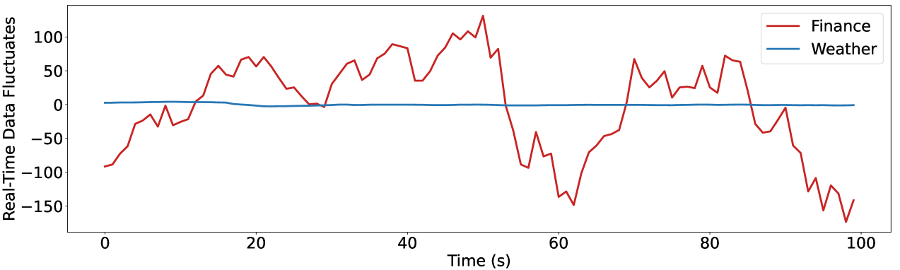
Figure 5: Visualization of the time series belongs to the Weather dataset and the finance subset in the M4 dataset. The temperature readings measured by the meteorological station are generally stable, whereas stock prices in financial markets fluctuate rapidly around the average value.

A.3 Metrics of Time Series Forecasting

In this paper, we mainly employ five widely used metrics to assess model performance, including Mean Squared Error (MSE), Mean Absolute Error (MAE), Mean Absolute Scaled Error (MSAE), Symmetric Mean Absolute Percentage Error (SMAPE), and Overall Weighted Average (OWA).
MSE measures the average of the squared differences between the predicted and actual values. MSE gives more weight to more significant errors because the errors are squared, thereby sensitive to outliers. Given $T$ time steps ground-truth time series signal $\mathbf{Y}=\left\{\mathbf{x}_{H+1},\ldots,\mathbf{x}_{H+T}\right\}\in\mathbb{R}^{T\times V}$ and prediction $\hat{\mathbf{Y}}=\left\{\hat{\mathbf{x}}_{H+1},\ldots,\hat{\mathbf{x}}_{H+T}\right\}\in\mathbb{R}^{T\times V}$, MSE is calculated as:

$$\operatorname{MSE}=\frac{1}{T}\sum_{i=1}^{T}\left(\mathbf{x}_{H+i}-\hat{\mathbf{x}}_{H+i}\right)^{2}.$$ (11)

MAE quantifies the average squared differences between predicted and actual values. It is less sensitive to outliers than MSE because it does not square the errors, treating all errors linearly. MAE is computed as:

$$\operatorname{MAE}=\frac{1}{T}\sum_{i=1}^{T}\left|\mathbf{x}_{H+i}-\hat{\mathbf{x}}_{H+i}\right|.$$ (12)

MSAE evaluates the accuracy of a model by scaling the absolute error relative to the actual values, which is calculated as:

$$\text{MSAE}=\frac{1}{T}\sum_{i=1}^{T}\frac{|\mathbf{x}_{H+i}-\hat{\mathbf{x}}_{H+i}|}{|\mathbf{x}_{H+i}|}.$$ (13)

SMAPE aims to provide a more balanced error with a symmetry formula, especially when the actual values approach zero. This helps mitigate the instability in MAPE when the actual values are small. SMAPE is calculated as:

$$\text{SMAPE}=\frac{1}{T}\sum_{i=1}^{T}\frac{2|\mathbf{x}_{H+i}-\hat{\mathbf{x}}_{H+i}|}{\mathbf{x}_{H+i}+|\hat{\mathbf{x}}_{H+i}|}.$$ (14)

OWA is commonly used for multiple tasks or criteria, and the importance of each task or metric differs. It allows for a balanced evaluation by adjusting the contribution of each task based on its relative importance. OWA is computed as:

$$\text{OWA}=\sum_{i=1}^{N}w_{i}\cdot v_{i},$$ (15)

where $N$ is the number of tasks (metrics), $w_{i}$ is the weight assigned to the $i$-th task (metric) and $\sum_{i=1}^{N}w_{i}=1$, $v_{i}$ is the evaluation result of the $i$-th task (metric).

Appendix B Model Analysis

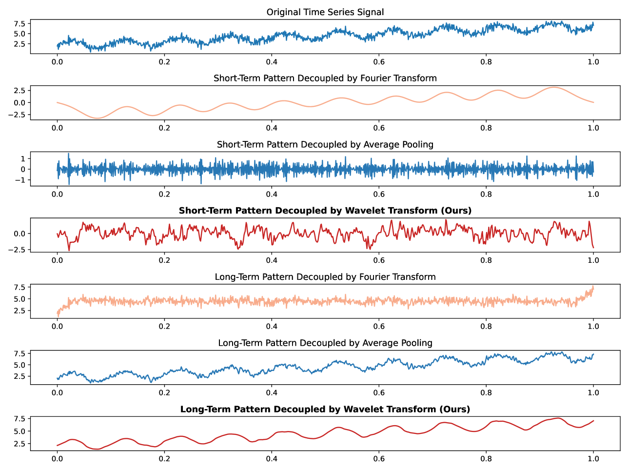
Figure 6: Visualization results of temporal patterns decoupled by our proposed wavelet-transform-based decoupling technique and other widely-used decoupling methods based on Fourier transform and average pooling.

B.1 Wavelet Transform

Our MSCNN employs the DauBechies 4 (DB4) wavelet transform with four vanishing moments to decouple low-frequency components $\mathbf{W}^{b}_{\text{low}}$ and high-frequency components $\{\mathbf{W}^{b}_{\text{high}\_i}\}_{i=1}^{w}$. The DB4 wavelet transform is widely used in time series signal processing due to its compact support and smoothness. Specifically, the DB4 wavelet transform decomposes the input time series via sequential decomposition and downsampling steps. In the decomposition step, the time series $\mathbf{X}=\left\{\mathbf{x}_{1},\ldots,\mathbf{x}_{H}\right\}\in\mathbb{R}^{H\times V}$ is progressively decomposed into multiple frequency bands with $w$ levels, encompassing both low-frequency and high-frequency components. At $i$-th decomposition level, the time series $\mathbf{X}$ is passed through low-pass filter $f^{i}_{\text{low}}$ and high-pass filter $f^{i}_{\text{high}}$ to generate the low-frequency approximation coefficients $\mathbf{a}_{i}$ and high-frequency detail coefficients $\mathbf{d}_{i}$:

$$\mathbf{a}_{i}[n]=\sum_{k=0}^{L-1}f^{i}_{\text{low}}[k]\cdot\mathbf{X}[2n-k],\quad\mathbf{d}_{i}[n]=\sum_{k=0}^{L-1}f^{i}_{\text{high}}[k]\cdot\mathbf{X}[2n-k],\quad n=1,2,\ldots,\left\lfloor\frac{H+L-1}{2}\right\rfloor,$$ (16)

where $L=8$ denotes the filter length. After $w$ decomposition levels, the outputs from these filters undergo downsampling by a factor of 2. The final approximation $\mathbf{a}_{w}$, which represents the smoothest features of the signal, serves as the low-frequency components $\mathbf{W}^{b}_{\text{low}}$. Meanwhile, the detail coefficients $\{\mathbf{d}_{i}\}_{i=1}^{w}$, which capture diverse high-frequency details or changes in the input time series, constitute the high-frequency components $\{\mathbf{W}^{b}_{\text{high}\_i}\}_{i=1}^{w}$.

Conversely, the inverse DB4 wavelet transform reconstructs the original signal through upsampling and reversed-order filtering. During the upsampling step, the approximation coefficients and detail coefficients are expanded by a factor of 2 to recover the original signal length. In the filtering step, the upsampled coefficients are convolved with the same low-pass and high-pass filters used during the decomposition in reverse order to reconstruct the time series signal:

$$\mathbf{X}=\sum_{i=1}^{w}\left(\tilde{\mathbf{a}}_{i}+\tilde{\mathbf{d}}_{i}\right).$$ (17)

Here, $\tilde{\mathbf{a}}_{i}$ and $\tilde{\mathbf{d}}_{i}$ represent reconstruction coefficients and details, which are calculated as follows:

$$\tilde{\mathbf{a}}_{i}[m]=\sum_{n}\tilde{f}^{i}_{\text{low}}[m-2n]\cdot\mathbf{a}_{i}[n],\quad\tilde{\mathbf{d}}_{i}[m]=\sum_{n}\tilde{f}^{i}_{\text{high}}[m-2n]\cdot\mathbf{d}_{i}[n],\quad m=1,2,\ldots,H.$$ (18)

$\tilde{f}^{i}_{\text{low}}$ (low-pass) and $\tilde{f}^{i}_{\text{high}}$ (high-pass), derived as time-reversed versions of the decomposition filter $f^{i}_{\text{low}}$ (low-pass) and $f^{i}_{\text{high}}$, as follows:

$$\tilde{f}^{i}_{\text{low}}[k]=f^{i}_{\text{low}}[L-1-k],\quad\tilde{f}^{i}_{\text{high}}[k]=f^{i}_{\text{high}}[L-1-k],\quad k=0,1,\ldots,L-1.$$ (19)

B.2 Visualizations of Decoupled Temporal Patterns

In this section, we compare our proposed wavelet-transform-based temporal pattern decoupling technique with other methods that employ Fourier transform and average pooling. Fig. 6 visualizes the decomposed short-term and long-term patterns. We can observe that our decoupling method achieves significantly better results than other decoupling methods. In particular, our method accurately captures short-term patterns that mirror the periodic fluctuations of the original time series, while effectively representing the overall trend in the long-term patterns.

B.3 Receptive Field of MSCNN

In CNNs, the receptive field refers to the region of the input associated with each output in a convolutional layer. The size of the receptive field determines how much of the input the network observes during convolution operations. In general, the receptive field of the output for a convolutional layer depends on the kernel size $k$, stride $s$, and the receptive field of the input $R_{\text{in}}$, which is formulated as:

$$R_{\text{out}}=R_{\text{in}}+(k-1)\times s.$$ (20)

In our MSCNN block, the features are divided into multiple branches and processed by parallel 3$\times$3 convolutional layers with an identical stride $s$=1. Given the features $\{\bar{\mathbf{F}}_{1},\ldots,\bar{\mathbf{F}}_{B}\}$ obtained from $B$ branches in Eq. (1), we assume that the receptive field of input features $R_{\text{in}}$=1 and $B$=4, and the receptive fields of multiple-branch features are $[3,5,7,9]$. Here, features with a small receptive field focus on short-term patterns, namely the periodic fluctuations, while features with a large receptive field focus on long-term patterns, namely the overall trend. Therefore, our proposed MSCNN can effectively capture both short-term and long-term patterns.

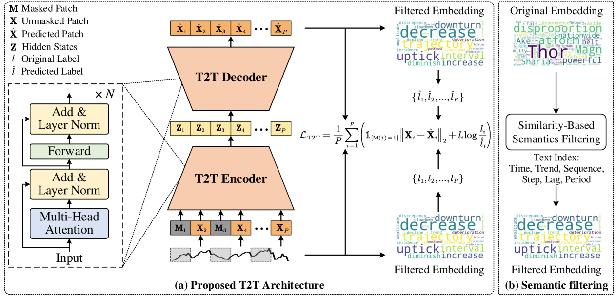
Figure 7: The diagram of our proposed Time-to-Text (T2T) module. The input time series is first divided into $P$ patches, with some patches randomly masked. These patches are then fed into the encoder and decoder to facilitate T2T’s accurate reconstruction and encourage T2T to learn meaningful semantic information by encouraging it to accurately predict the semantic labels of the time patches.

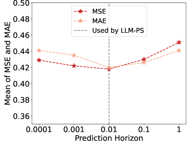
Figure 8: Parametric sensitivities of $\lambda$ in Eq. 9.

B.4 Time-to-Text Module

In this paper, we design the Time-to-Text (T2T) module to extract semantic information from the input time series. We follow (Hsu et al., 2021) and construct the T2T with an encoder-decoder architecture, where both the encoder and decoder are stacked by transformer layers, as shown in Fig. 7.
Model Configuration. In the T2T module, the encoder and decoder contain 4 and 1 transformer layer, respectively. Each transformer layer consists of the multi-head attention layer, feedforward network, and layer normalization. The patch size, hidden dimension, feedforward hidden size, and output size are set to 24, 96, 384, and 24, respectively.
Training Setups. During training, the T2T module is optimized by Adam, where the learning rate is set to 0.001. The masking ratio of input time series patches is set to 0.75.
Time Series Patching. The input series $\mathbf{X}=\left\{\mathbf{x}_{1},\ldots,\mathbf{x}_{H}\right\}\in\mathbb{R}^{H\times V}$ is divided into $P$ overlapping patches $\{\mathbf{X}_{i}\}^{P}_{i=1}$, where $\mathbf{X}_{i}\in\mathbb{R}^{L\times V}$. The patch length is given by $L=\frac{H+O}{P}$, and $O$ denotes the overlap length between consecutive patches.
Semantic Filtering. In the LLM word embeddings, there are numerous inrelevant semantic information for Time Series Forecasting (TSF). As shown in Fig. 7, the original word embeddings $\mathbf{E}_{\text{ori}}\in\mathbb{R}^{W\times D}$ (where $W$ and $D$ are the length and dimension of $\mathbf{E}_{\text{ori}}$) of the GPT2 model includes embedding with corresponding word such as “Thro”, “Magn”, and “belt”, which are irrelevant to TSF. To facilitate T2T in extracting valuable semantic information for TSF, we filter the LLM word embeddings based on text indices relevant to TSF.

Specifically, given the text indices $\{t_{i}\}_{i}^{I}$ ($I$ denotes the number of text indices) corresponding to the TSF, the similarities between their word embeddings $\hat{\mathbf{E}}=\{\mathbf{E}_{\text{ori}}[t_{i}]\}_{i=1}^{I}$ and LLM word embeddings $\mathbf{E}_{\text{ori}}$ are computed as follows:

$$\mathbf{s}=\frac{\hat{\mathbf{E}}\cdot\mathbf{E}_{\text{ori}}}{\|\hat{\mathbf{E}}\|_{2}\|\mathbf{E}_{\text{ori}}\|_{2}}.$$ (21)

Then, we select the top 100 most similar word embeddings as the final word embeddings $\mathbf{E}$ for T2T training.

B.5 Parameter Sensitivity Analysis

The LLM-PS equation (Eq. (9)) in our model has one tuning parameter, denoted as $\lambda$. We analyze its sensitivities on the ETTh1 dataset by varying $\lambda$ within the range of $\{0.0001,0.001,0.01,0.1,1\}$ and observe the mean MSE/MAE across predict lengths spanning $\{96,192,336,720\}$, as shown in Fig. 8. Despite the large fluctuations in $\lambda$, the MSE/MAE curve of our LLM-PS remains relatively stable. These results demonstrate the robustness of our LLM-PS against parameter variations. Furthermore, our LLM-PS achieves its best performance when $\lambda=0.01$, so we adopt this parameter configuration in our method.

References

- Angryk et al. (2020) Angryk, R. A., Martens, P. C., Aydin, B., Kempton, D., Mahajan, S. S., Basodi, S., Ahmadzadeh, A., Cai, X., Filali Boubrahimi, S., Hamdi, S. M., et al. Multivariate time series dataset for space weather data analytics. Scientific Data, 7(1):227, 2020.
- Bai et al. (2018) Bai, S., Kolter, J. Z., and Koltun, V. An empirical evaluation of generic convolutional and recurrent networks for sequence modeling. arXiv preprint arXiv:1803.01271, 2018.
- Brown et al. (2020) Brown, T., Mann, B., Ryder, N., Subbiah, M., Kaplan, J. D., Dhariwal, P., Neelakantan, A., Shyam, P., Sastry, G., Askell, A., et al. Language models are few-shot learners. Advances in Neural Information Processing Systems (NeurIPS), 33:1877–1901, 2020.
- (4) Cao, D., Jia, F., Arik, S. O., Pfister, T., Zheng, Y., Ye, W., and Liu, Y. Tempo: Prompt-based generative pre-trained transformer for time series forecasting. In International Conference on Learning Representations (ICLR).
- Challu et al. (2022) Challu, C., Olivares, K. G., Oreshkin, B. N., Garza, F., Mergenthaler, M., and Dubrawski, A. N-HiTs: Neural hierarchical interpolation for time series forecasting. arXiv preprint arXiv:2201.12886, 2022.
- Chen et al. (2024) Chen, C., Oliveira, G., Noghabi, H. S., and Sylvain, T. Llm-ts integrator: Integrating llm for enhanced time series modeling. arXiv preprint arXiv:2410.16489, 2024.
- Cheng et al. (2023) Cheng, M., Liu, Q., Liu, Z., Zhang, H., Zhang, R., and Chen, E. Timemae: Self-supervised representations of time series with decoupled masked autoencoders. arXiv preprint arXiv:2303.00320, 2023.
- Chung et al. (2023) Chung, H., Kim, J., Kwon, J.-m., Jeon, K.-H., Lee, M. S., and Choi, E. Text-to-ecg: 12-lead electrocardiogram synthesis conditioned on clinical text reports. In IEEE International Conference on Acoustics, Speech and Signal Processing (ICASSP), pp. 1–5. IEEE, 2023.
- Cleveland et al. (1990) Cleveland, R. B., Cleveland, W. S., McRae, J. E., Terpenning, I., et al. Stl: A seasonal-trend decomposition. J. off. Stat, 6(1):3–73, 1990.
- Cochran et al. (1967) Cochran, W. T., Cooley, J. W., Favin, D. L., Helms, H. D., Kaenel, R. A., Lang, W. W., Maling, G. C., Nelson, D. E., Rader, C. M., and Welch, P. D. What is the fast fourier transform? Proceedings of the IEEE, 55(10):1664–1674, 1967.
- Das et al. (2023) Das, A., Kong, W., Leach, A., Sen, R., and Yu, R. Long-term forecasting with TiDE: Time-series dense encoder. arXiv preprint arXiv:2304.08424, 2023.
- Défossez et al. (2023) Défossez, A., Copet, J., Synnaeve, G., and Adi, Y. High fidelity neural audio compression. Transactions on Machine Learning Research (TMLR), 2023.
- Devlin et al. (2018) Devlin, J., Chang, M., Lee, K., and Toutanova, K. BERT: pre-training of deep bidirectional transformers for language understanding. CoRR, abs/1810.04805, 2018.
- Gao et al. (2019) Gao, S.-H., Cheng, M.-M., Zhao, K., Zhang, X.-Y., Yang, M.-H., and Torr, P. Res2net: A new multi-scale backbone architecture. IEEE Transactions on Pattern Analysis and Machine Intelligence (TPAMI), 43(2):652–662, 2019.
- Gu et al. (2022) Gu, A., Goel, K., and Ré, C. Efficiently modeling long sequences with structured state spaces. In International Conference on Learning Representations (ICLR), 2022.
- He et al. (2016) He, K., Zhang, X., Ren, S., and Sun, J. Deep residual learning for image recognition. In Proceedings of the IEEE Conference on Computer Vision and Pattern Recognition (CVPR), pp. 770–778, 2016.
- Hochreiter & Schmidhuber (1997) Hochreiter, S. and Schmidhuber, J. Long short-term memory. Neural Comput (NC), 1997.
- Hsu et al. (2021) Hsu, W.-N., Bolte, B., Tsai, Y.-H. H., Lakhotia, K., Salakhutdinov, R., and Mohamed, A. Hubert: Self-supervised speech representation learning by masked prediction of hidden units. IEEE/ACM Transactions on Audio, Speech, and Language Processing (TASLR), 29:3451–3460, 2021.
- Hu et al. (2021) Hu, E. J., Shen, Y., Wallis, P., Allen-Zhu, Z., Li, Y., Wang, S., Wang, L., and Chen, W. Lora: Low-rank adaptation of large language models. arXiv preprint arXiv:2106.09685, 2021.
- Hyndman (2018) Hyndman, R. Forecasting: principles and practice. OTexts, 2018.
- Jin et al. (2024) Jin, M., Wang, S., Ma, L., Chu, Z., Zhang, J., Shi, X., Chen, P.-Y., Liang, Y., Li, Y.-f., Pan, S., et al. Time-llm: Time series forecasting by reprogramming large language models. In International Conference on Learning Representations (ICLR), 2024.
- Kowsher et al. (2024) Kowsher, M., Sobuj, M. S. I., Prottasha, N. J., Alanis, E. A., Garibay, O. O., and Yousefi, N. Llm-mixer: Multiscale mixing in llms for time series forecasting. arXiv preprint arXiv:2410.11674, 2024.
- Liu et al. (2024a) Liu, P., Guo, H., Dai, T., Li, N., Bao, J., Ren, X., Jiang, Y., and Xia, S.-T. Calf: Aligning llms for time series forecasting via cross-modal fine-tuning. arXiv preprint arXiv:2403.07300, 2024a.
- Liu et al. (2024b) Liu, Y., Hu, T., Zhang, H., Wu, H., Wang, S., Ma, L., and Long, M. iTransformer: Inverted transformers are effective for time series forecasting. International Conference on Learning Representations (ICLR), 2024b.
- Makridakis et al. (2018) Makridakis, S., Spiliotis, E., and Assimakopoulos, V. The m4 competition: Results, findings, conclusion and way forward. International Journal of Forecasting (IJF), 34(4):802–808, 2018.
- Moody & Mark (2001) Moody, G. B. and Mark, R. G. The impact of the mit-bih arrhythmia database. IEEE Engineering in Medicine and Biology Magazine (IEMBM), 20(3):45–50, 2001.
- Nie et al. (2023) Nie, Y., H. Nguyen, N., Sinthong, P., and Kalagnanam, J. A time series is worth 64 words: Long-term forecasting with transformers. In International Conference on Learning Representations (ICLR), 2023.
- Oreshkin et al. (2019a) Oreshkin, B. N., Carpov, D., Chapados, N., and Bengio, Y. N-beats: Neural basis expansion analysis for interpretable time series forecasting. arXiv preprint arXiv:1905.10437, 2019a.
- Oreshkin et al. (2019b) Oreshkin, B. N., Carpov, D., Chapados, N., and Bengio, Y. N-BEATS: Neural basis expansion analysis for interpretable time series forecasting. International Conference on Learning Representations (ICLR), 2019b.
- Patton (2013) Patton, A. Copula methods for forecasting multivariate time series. Handbook of economic forecasting, 2:899–960, 2013.
- Radford et al. (2019) Radford, A., Wu, J., Child, R., Luan, D., Amodei, D., Sutskever, I., et al. Language models are unsupervised multitask learners. OpenAI blog, 1(8):9, 2019.
- Rubenstein et al. (2023) Rubenstein, P. K., Asawaroengchai, C., Nguyen, D. D., Bapna, A., Borsos, Z., Quitry, F. d. C., Chen, P., Badawy, D. E., Han, W., Kharitonov, E., et al. Audiopalm: A large language model that can speak and listen. arXiv preprint arXiv:2306.12925, 2023.
- Salinas et al. (2020) Salinas, D., Flunkert, V., Gasthaus, J., and Januschowski, T. Deepar: Probabilistic forecasting with autoregressive recurrent networks. International Journal of Forecasting (IJF), 36(3):1181–1191, 2020.
- Taylor & Letham (2018) Taylor, S. J. and Letham, B. Forecasting at scale. The American Statistician, 72(1):37–45, 2018.
- Touvron et al. (2023) Touvron, H., Lavril, T., Izacard, G., Martinet, X., Lachaux, M.-A., Lacroix, T., Rozière, B., Goyal, N., Hambro, E., Azhar, F., et al. Llama: Open and efficient foundation language models. arXiv preprint arXiv:2302.13971, 2023.
- Trindade (2015) Trindade, A. ElectricityLoadDiagrams20112014. UCI Machine Learning Repository, 2015. DOI: https://doi.org/10.24432/C58C86.
- Van Den Oord et al. (2017) Van Den Oord, A., Vinyals, O., et al. Neural discrete representation learning. Advances in Neural Information Processing Systems (NeurIPS), 30, 2017.
- Wang et al. (2022) Wang, H., Peng, J., Huang, F., Wang, J., Chen, J., and Xiao, Y. MICN: Multi-scale local and global context modeling for long-term series forecasting. In International Conference on Learning Representations (ICLR), 2022.
- Wang et al. (2024) Wang, S., Wu, H., Shi, X., Hu, T., Luo, H., Ma, L., Zhang, J. Y., and ZHOU, J. Timemixer: Decomposable multiscale mixing for time series forecasting. In International Conference on Learning Representations (ICLR), 2024.
- Wen et al. (2023) Wen, Q., Zhou, T., Zhang, C., Chen, W., Ma, Z., Yan, J., and Sun, L. Transformers in time series: a survey. In Proceedings of the Thirty-Second International Joint Conference on Artificial Intelligence (IJCAI), pp. 6778–6786, 2023.
- Woo et al. (2022) Woo, G., Liu, C., Sahoo, D., Kumar, A., and Hoi, S. C. H. ETSformer: Exponential smoothing transformers for time-series forecasting. arXiv preprint arXiv:2202.01381, 2022.
- Wu et al. (2021) Wu, H., Xu, J., Wang, J., and Long, M. Autoformer: Decomposition transformers with Auto-Correlation for long-term series forecasting. In Advances in Neural Information Processing Systems (NeurIPS), 2021.
- Wu et al. (2023a) Wu, H., Hu, T., Liu, Y., Zhou, H., Wang, J., and Long, M. TimesNet: Temporal 2d-variation modeling for general time series analysis. In International Conference on Learning Representations (ICLR), 2023a.
- Wu et al. (2023b) Wu, H., Hu, T., Liu, Y., Zhou, H., Wang, J., and Long, M. Timesnet: Temporal 2d-variation modeling for general time series analysis. In International Conference on Learning Representations (ICLR), 2023b.
- Wu et al. (2023c) Wu, H., Zhou, H., Long, M., and Wang, J. Interpretable weather forecasting for worldwide stations with a unified deep model. Nature Machine Intelligence (NMI), 5(6):602–611, 2023c.
- Xue & Salim (2023) Xue, H. and Salim, F. D. Promptcast: A new prompt-based learning paradigm for time series forecasting. IEEE Transactions on Knowledge and Data Engineering (TKDE), 2023.
- Zeng et al. (2023) Zeng, A., Chen, M., Zhang, L., and Xu, Q. Are transformers effective for time series forecasting? In Proceedings of the AAAI Conference on Artificial Intelligence, volume 37, pp. 11121–11128, 2023.
- Zhang (2019) Zhang, D. Wavelet transform. Fundamentals of Image Data Mining: Analysis, Features, Classification and Retrieval, pp. 35–44, 2019.
- Zhang & Qi (2005) Zhang, G. P. and Qi, M. Neural network forecasting for seasonal and trend time series. European Journal of Operational Research (EJOR), 160(2):501–514, 2005.
- Zhang et al. (2024a) Zhang, X., Chowdhury, R. R., Gupta, R. K., and Shang, J. Large language models for time series: A survey. arXiv preprint arXiv:2402.01801, 2024a.
- Zhang et al. (2024b) Zhang, X., Zhang, D., Li, S., Zhou, Y., and Qiu, X. Speechtokenizer: Unified speech tokenizer for speech language models. In International Conference on Learning Representations (ICLR), 2024b.
- Zhang & Yan (2023a) Zhang, Y. and Yan, J. Crossformer: Transformer utilizing cross-dimension dependency for multivariate time series forecasting. In International Conference on Learning Representations (ICLR), 2023a.
- Zhang & Yan (2023b) Zhang, Y. and Yan, J. Crossformer: Transformer utilizing cross-dimension dependency for multivariate time series forecasting. In International Conference on Learning Representations (ICLR), 2023b.
- Zhou et al. (2021a) Zhou, H., Zhang, S., Peng, J., Zhang, S., Li, J., Xiong, H., and Zhang, W. Informer: Beyond efficient transformer for long sequence time-series forecasting. In Proceedings of the AAAI Conference on Artificial Intelligence, volume 35, pp. 11106–11115, 2021a.
- Zhou et al. (2021b) Zhou, H., Zhang, S., Peng, J., Zhang, S., Li, J., Xiong, H., and Zhang, W. Informer: Beyond efficient transformer for long sequence time-series forecasting. In Proceedings of the AAAI Conference on Artificial Intelligence, volume 35, pp. 11106–11115, 2021b.
- Zhou et al. (2022) Zhou, T., Ma, Z., Wen, Q., Wang, X., Sun, L., and Jin, R. Fedformer: Frequency enhanced decomposed transformer for long-term series forecasting. In International Conference on Machine Learning (ICML), pp. 27268–27286. PMLR, 2022.
- Zhou et al. (2023a) Zhou, T., Niu, P., Sun, L., Jin, R., et al. One fits all: Power general time series analysis by pretrained lm. Advances in Neural Information Processing Systems (NeurIPS), 36:43322–43355, 2023a.
- Zhou et al. (2023b) Zhou, T., Niu, P., Wang, X., Sun, L., and Jin, R. One Fits All: Power general time series analysis by pretrained lm. Advances in Neural Information Processing Systems (NeurIPS), 36, 2023b.