Parameter estimation of gravitational-wave signals with frequency-dependent antenna responses and higher-modes

Abstract

We implement frequency-dependent antenna responses and develop likelihood classes (standard likelihood, multibanded likelihood, and the relative binning (RB) likelihood) capable of handling the same within the framework of Bilby. We validate the approximate likelihoods by comparing them with the exact likelihood for a GW170817-like signal (signal-to-noise ratio   1900) containing higher-order modes of radiation. We use the relative-binning likelihood to perform parameter estimation (PE) for a GW170817-like signal, including Earth-rotation effects, detector-size effects, and higher-order modes. We study the system in several detector networks consisting of a single 40 km Cosmic Explorer, a 20 km CE and a present-generation detector at A+ sensitivity. The PE runs with RB take around a day to complete on a typical cluster.

1 Introduction

The discovery of gravitational waves (GWs) has enabled the study of compact binary coalescences (CBCs) comprising black holes and neutron stars [1, 2, 3, 4, 5]. The LIGO-Virgo-KAGRA (LVK) [6, 7, 8] collaboration has confidently detected around 90 compact CBCs with 200 more candidates from the present observing run [9]. These detections have tested our understanding of gravity, cosmology, and astrophysics [10, 11, 12]. The proposed next-generation ground-based detectors, such as the Cosmic Explorer (CE) [13] and Einstein Telescope (ET) [14], promise an exciting era of gravitational wave detections, offering sensitivities that extend well beyond current capabilities. The next-generation observatories are sensitive enough to detect signals from sources at cosmological distances and provide precise measurements of their parameters which are expected to play a pivotal role in advancing our understanding of fundamental physics, astrophysics, and cosmology [15, 16, 17].

To understand the full potential of these next-generation detectors we need estimates of how well various parameters can be measured. Using conventional Bayesian parameter estimation (PE) is challenging, given the large number of detections ($\mathcal{O}\sim 10^{5}-10^{6}$) [18] per year, some with signal-to-noise ratios (SNRs) greater than 1000. Moreover, signals are long and we need to incorporate corrections due to Earth’s rotation at low frequencies and detector-size at high frequencies [19, 20]. Ignoring these effects is known to cause biases at high SNRs [21]. Higher-order modes of radiation become non-negligible at higher SNRs making Bayesian PE more complex and computationally expensive.

Fisher information matrices offer a computationally cheap way to estimate the uncertainties in measured parameters. Effects on localization due to Earth’s rotation have been extensively studied in this framework [22, 23]. Several constraints on cosmological parameters have also been given using Fisher matrices [24]. This method has also been used for parameter estimation of intermediate mass black holes in a network of detectors and the results agree with Bayesian parameter estimation to an order of magnitude in the parameter space of interest [25]. However, no general Fisher matrix approach taking into account all the effects due to Earth’s rotation, the detector-size and higher modes exist in literature. Also, this approximation becomes non-trivial if the parameter space has multimodalities.

Bayesian parameter estimation does not suffer from the shortcomings of Fisher information matrices but is computationally expensive. A recent paper by Baker et. al. [26] highlights the computational challenges of inference in next-generation detectors. Nearly all Bayesian PE in next-generation detectors involves approximating the likelihood. Pre-merger localization of compact-binary sources in next-generation networks [27] have been studied using relative binning [28]. Reduced order models taking into account only the amplitude modulations due to Earth-rotation using BNS signals lasting 90 minutes in-band from 5 Hz to 2048 Hz have been constructed for a network of detectors [29]. A recent paper highlights challenges Bayesian PE with effects due to Earth’s rotation and detector-size effects have been implemented [21] in the framework of the multibanding approximation [30]. Bayesian PE with relative binning has also been used to measure tidal deformabilities in ET [31]. Similar work has been done for Laser Interferometer Space Antenna (LISA) [32].

In this paper, we develop a generalized framework using Bilby [33] to generate waveforms including effects due to Earth-rotation, finite-size of detectors and higher modes. We develop four new likelihood classes: the exact likelihood including all effects; the multibanding likelihood capable of handling all effects; a relative binning likelihood capable of handling the dominant mode of radiation; a mode-by-mode relative binning likelihood capable of handling all modes of radiation. We do illustrative PE for two GW170817-like [3] sources in four network configurations: a single 40 km CE, a network of LIGO-India and a 40 km CE; a network of a 40 km long and a 20 km long CE; and a network comprising of all detectors. We study the roles played by the higher-order multiples of radiation in these networks.

The rest of the paper is organized as follows. In section 2, we describe our implementations and provide code snippets describing how to use them. In the next section 3 we describe the sources, waveform family and the detection networks used in the study. Finally we validate our methods and present the results of our study in section 4.

2 Methods

2.1 Frequency-dependent antenna responses

In general relativity, the metric perturbation $h_{ij}$ corresponding to the GW in the transverse traceless gauge is characterized by two polarization components $h_{+}$ and $h_{\times}$ as described by [34],

$$h_{ij}=h_{+}e^{+}_{ij}+h_{\times}e^{\times}_{ij}$$ (1)

The GW polarization tensors ($e^{+}_{ij},e^{\times}_{ij}$) can be expressed in terms of basis vectors in the transverse plane ($e^{1}_{i},e^{2}_{j}$) given by,

$$e^{+}_{ij}:=e^{1}_{i}e^{1}_{j}-e^{2}_{i}e^{2}_{j}$$ (2)

$$e^{\times}_{ij}:=e^{1}_{i}e^{2}_{j}+e^{2}_{i}e^{1}_{j}$$ (3)

The detected GW strain as a function of time ($t$) can be expressed as $d(t)=h_{D}(t)+n(t)$, where $n$ represents noise and $h_{D}$ is the GW signal at the detector obtained by the product of the detector tensor ($D^{ij}$) [35] and the metric perturbations. In terms of the polarization components, the strain at the detector is expressed as,

$$h_{D}(t-t_{c};\Theta)=\sum_{i=+,\times}F_{i}(t-t_{c},f;\xi,I)h_{i}(t-t_{c};\theta,D_{L},\theta_{JN},\phi_{c})$$ (4)

where

$$F_{+}(t-t_{c},f;\xi,I):=D^{ij}(t-t_{c},f;\xi,I)e^{+}_{ij}(t-t_{c};\xi)$$ (5)

$$F_{\times}(t-t_{c},f;\xi,I):=D^{ij}(t-t_{c},f;\xi,I)e^{\times}_{ij}(t-t_{c};\xi)$$ (6)

Here $f$ denotes the frequency, $t_{c}$ is the arrival time of the frequency corresponding to the merger at the geocenter and $I$ is the position and orientation of the interferometer. The angle uniquely defining $e^{1}_{i},e^{2}_{j}$ in the transverse plane is the polarization angle ($\psi$). The right ascension ($\rm RA$), declination ($\rm dec$), $\psi$ and $t_{c}$ is collectively denoted by $\xi:=({\rm RA},{\rm dec},\psi,t_{c})$.

The signals are short-lived for current-generation ground-based detectors and so $t\simeq t_{c}$, where $t_{c}$ is the arrival time of the GW at the detector. The detector tensor is also a constant tensor with no dependence on frequency or the direction of the source ($\xi$). Thus for the present generation detectors,

$$F_{+}(0,0;\xi,I):=D^{ij}(0,0;I)e^{+}_{ij}(0;\xi)$$ (7)

$$F_{\times}(0,0;\xi,I):=D^{ij}(0,0;I)e^{\times}_{ij}(0;\xi)$$ (8)

Thus, for a given pair of source and a detector the antenna-response functions $F_{+}$ and $F_{\times}$ are constants with no frequency dependence.

Loud sources in next-generation detectors observed from a frame co-rotating with the Earth (the rest-frame of ground-based detectors) shift in the sky, changing the antenna-response function as the signal evolves. The waveform polarizations depend on the intrinsic source parameters like chirp mass ($\mathcal{M}$), mass ratio ($q$) and aligned-spin parameters ($\chi_{1},\chi_{2}$) collectively denoted by $\theta:={\mathcal{M},q,\chi_{1}\chi_{2}}$, the luminosity distance $D_{L}$, the inclination angle $\theta_{\rm JN}$ and the coalescence phase $\phi_{c}$. Collectively, these parameters are represented as $\Theta:=(\xi,\theta,D_{L},\theta_{\rm JN},\phi_{c})$. The earth’s rotation also introduces an integrated Doppler shift as the time delay between the detector and the geocenter is different for various frequencies corresponding to the CBC signal since lower frequencies arrive at earlier times. The effect on the beam patterns and the Doppler effect combined are called Earth-rotation effects in this paper.

The long-wavelength approximation breaks down for a 40 km long detector at high frequencies. For finite wavelengths, the measured strain depends not only on when wavefronts pass through the vertex of the interferometer, but also when it passes through the ends of the arms [19, 20], which introduces an additional dependence on the direction of the wave propagation which in turn depends on the (time-changing) wavelength (or frequency).This effect is referred to as the detector-size effect in this paper.

Thus, for current-generation detectors we need the complete time-frequency dependence as in equation 12, with the $D^{ij}$ having additional frequency and directional dependence, $e^{+,\times}_{ij}$ having temporal dependence and an integrated Doppler shift. Ignoring these effects may introduce systematic biases in parameter estimation (PE) [21].

Time ($\tau:=t-t_{c}$) and frequency are not independent parameters for a GW from a CBC and are related by an invertible function. Parameter estimation is often performed in the frequency domain, necessitating the Fourier transformation of equation 12 to the frequency domain. Analytical computation of the Fourier transform is challenging without approximations. We assume that $h_{i}$’s oscillate rapidly compared to the antenna responses (the stationary phase approximation). We can therefore, take the Fourier transform of the waveform polarizations and convert the times in the antenna response to frequency using the time-frequency relation for a CBC signal computed up to second post-Newtonian (PN) [36] order. While this method is approximate, it provides sufficient accuracy for practical applications. Details of this method can be found in [21].

The GW polarizations are often expressed in terms of spin-weighted spherical harmonics.

$$h_{D}(f;\Theta)=\sum_{i=+,\times}\sum_{m=-l}^{l}F_{i}(\tau(m,f),f;\xi)\sum_{l=2}^{\infty}h^{lm}_{+}(f;\theta,D_{L},\theta_{\rm JN},\phi_{c},t_{c})$$ (9)

where the real-valued $h^{lm}_{+}$ and $h^{lm}_{\times}$ are related to the complex valued $h^{lm}_{+}(f)$ and the spin-2 weighted spherical harmonics ${}_{-2}Y_{lm}$ as

$$h^{lm}_{+}(f;\theta,D_{L},\theta_{\rm JN},\phi_{c},t_{c})-ih^{lm}_{\times}(f;\theta,D_{L},\theta_{\rm JN},\phi_{c},t_{c})=_{-2}Y_{lm}(\theta_{\rm JN},\phi_{c})h_{lm}(f;\theta,D_{L},t_{c})$$ (10)

In PN theory the time-to-merger for an azimuthal mode $m$ from a frequency $f$, is equivalent to the time to merger of a $m=2$ mode from a frequency $2f/m$ [37, 38]. So the antenna-responses when expressed in terms of frequencies depend on the azimuthal wave number $m$. We implement all functions and classes this paper requires in a cloned version of Bilby. The time-frequency relation for mode $m$ is implemented by a function named calculate_time_to_merger_for_any_mode in gw.utils and this is typically 30 times faster than the method calculate_time_to_merger tested on an Apple M3 Pro. The antenna patterns can be quickly computed as follows:

⬇

1>>> times_to_coalescence = gwutils.calculate_time_to_merger_for_any_mode(frequencies, mass1, mass2, chi1, chi2, mode=2, safety=1)

2>>> fps, fcs = ifo.frequency_dependent_antenna_response(ra, dec, time, psi, times_to_coalescence, frequencies, start_time, earth_rotation_time_delay = True, earth_rotation_beam_patterns = True, finite_size =True)

The arrays fps and fcs represent the plus and cross-polarization components, corresponding to the frequencies in the frequencies array. Parameters mass1, mass2, chi1, chi2,RA, dec, time, psi, and start_time denote the primary mass, secondary mass, primary spin, secondary spin, right ascension, declination, geocentric time, polarization angle, and the signal start time, respectively. The start time is the difference between the geocentric time and the duration of the signal plus any user-defined offset. The array times_to_coalescence specifies the times to merger for each frequency. The remaining parameters are boolean values set to true if the user wants all effects in the antenna responses. The waveform can be generated as follows:

⬇

1>>> waveform_generator = bilby.gw.WaveformGenerator(duration, sampling_frequency, frequency_domain_source_model=bilby.gw.source.lal_binary_black_hole_individual_modes, parameter_conversion=bilby.gw.conversion.convert_to_lal_binary_black_hole_parameters, waveform_arguments=dict(waveform_approximant=waveformname, reference_frequency=reference_frequency, minimum_frequency=minimum_frequency, mode_array=mode_array))

2>>> ifo = bilby.gw.detector.InterferometerList([‘CE’])[0]

3>>> frequencies = waveform_generator.frequency_array

4>>> parameters, _ = waveform_generator.parameter_conversion(injection_parameters)

5>>> waveform_polarizations = waveform_generator.frequency_domain_strain(converted_injection_parameters)

6>>> h[idxs_above_minimum_frequency] = ifo.get_detector_response_for_frequency_dependent_antenna_response(waveform_polarizations, parameters, start_time, frequencies, earth_rotation_time_delay, earth_rotation_beam_patterns,finite_size)’

Here bilby.gw.source.lal_binary_black_hole_individual_mode is a new frequency domain source model that creates a dictionary of the plus and cross polarizations for every mode of radiation. For computational efficiency, modes with the same azimuthal number $m$ are grouped, as they share the same antenna response. An exception is made for relative binning, where all modes are processed individually, as discussed in later sections.

2.2 Sampling the Likelihood

Bayesian parameter estimation depends on calculating the posterior probability distribution $p(\Theta|d)$ from the data $d$.

$$p(\Theta|d):=\frac{\mathcal{L}(\Theta|d)p(\Theta)}{\mathcal{Z}}$$ (11)

The prior denoted by $p(\Theta)$ is predetermined, and the evidence $\mathcal{Z}$ is the integral of the numerator over all data and is just a normalization constant. The likelihood assuming that noise is stationary and gaussian is given by $\mathcal{L}(\Theta|d):=p(d|\Theta):=\exp(-{\rm\big{<}}d-h|d-h{\rm\big{>}})\propto\exp(2{\rm\big{<}}h|d{\rm\big{>}}-{\rm\big{<}}h|h{\rm\big{>}})$ where ${\rm\big{<}}a|b{\rm\big{>}}=4\leavevmode\nobreak\ \text{Re}\int_{0}^{\infty}\frac{a^{*}(f)b(f)}{S_{n}(f)}df$ and $S_{n}(f)$ is the one-sided power spectral density. This likelihood is implemented as GravitationalWaveTransientNextGeneration in bilby.gw.likelihood.

⬇

1 >>> likelihood = bilby.gw.likelihood.GravitationalWaveTransientNextGeneration(interferometers=ifos, waveform_generator=waveform_generator, priors=priors_basic, distance_marginalization=False, phase_marginalization=False, time_reference=‘geocent’, earth_rotation_time_delay = True, earth_rotation_beam_patterns = True, finite_size = True,)’

We consider a frequency band of 5 Hz to 2048 Hz and so we set the sampling rate to 4096 Hz. For a GW170817-like signal, the dominant mode of radiation $h_{(+,\times)}^{2,2}$, lasts in-band for approximately 2 hours, requiring waveform evaluations at $10^{7}$ points. We need to calculate the waveform for each azimuthal mode m which takes around 10s on a single CPU. Computing the waveform for three azimuthal modes (m=2,3,4) takes approximately 30 seconds on a single CPU. Sampling the likelihood using a nested sampler like dynesty requires around $10^{8}$ waveform evaluations for high SNRs and is computationally prohibitive.

To accelerate likelihood evaluations, we employ two approximations: multibanding and relative binning, described in subsequent sections.

2.2.1 The Multibanding Approximation

The multibanding approximation [30] is a form of adaptive sampling that divides the entire frequency range into overlapping frequency bands where the start and end frequencies depend on the sequence of durations controlled by an accuracy factor. The duration should be computed using the highest azimuthal mode. This approximation was used to do parameter estimation of signals in Cosmic Explorer containing the dominant $h_{(+,\times)}^{2,2}$ mode [21]. However unlike [21], we compute the antenna response at every banded frequency point instead of every 4 seconds, making the algorithm more accurate without trading-off performance. We implement this approximation as MBGravitationalWaveTransientNextGeneration, a subclass of MBGravitationalWaveTransient in bilby.gw.likelihood.

⬇

1>>> search_waveform_generator_MB = bilby.gw.WaveformGenerator(duration=duration, sampling_frequency=sampling_frequency, frequency_domain_source_model=bilby.gw.source.binary_black_hole_individual_modes_frequency_sequence, parameter_conversion=bilby.gw.conversion.convert_to_lal_binary_black_hole_parameters, waveform_arguments=dict(waveform_approximant=waveformname, reference_frequency=reference_frequency, minimum_frequency=minimum_frequency, mode_array=mode_array))

2>>> likelihood_MB = bilby.gw.likelihood.MBGravitationalWaveTransientNextGeneration(interferometers=ifos, waveform_generator=search_waveform_generator_MB, priors=priors_MB, reference_chirp_mass=detector_frame_chirp_mass-1e-5, linear_interpolation=True, distance_marginalization=False,phase_marginalization=False, time_reference=‘geocent’, accuracy_factor = 5, highest_mode = 4, earth_rotation_time_delay = True, earth_rotation_beam_patterns = True, finite_size = True)’

The source model binary_black_hole_individual_modes_frequency_sequence can generate waveform polarizations for every azimuthal mode given an arbitrary frequency array. The reference_chirp_mass is an approximate value of chirp mass required for multibanding. The highest_mode should be set to the highest azimuthal mode. The accuracy_factor is a tunable parameter which controls the number of bands and hence the accuracy of the approximation (Referred to $L$ in [30]). A value of 5 results in errors in log-likelihood less than unity. This approximation due to adaptive frequency binning needs only $10^{5}$ evaluations per waveform resulting in a speed-up of $\mathcal{O}$($10^{2}$).

2.2.2 The Relative Binning Approximation

The relative binning technique accelerates parameter estimation by leveraging the smooth variation of waveform ratios across neighboring points in the parameter space. The waveform corresponding to the maximum likelihood estimate is selected as the fiducial waveform, serving as the reference for constructing approximations. Waveforms at nearby points in the parameter space are computed by applying piecewise linear modifications to the fiducial waveform, significantly reducing the computational overhead of waveform generation. This approach achieves speed-ups of up to $\mathcal{O}(10^{3})$ with minimal loss of accuracy [39, 40]. This method is implemented as RelativeBinningGravitationalWaveTransientNextGeneration in bilby.gw.likelihood.

⬇

1>>> search_waveform_generator_RB = bilby.gw.WaveformGenerator(duration=duration, sampling_frequency=sampling_frequency, frequency_domain_source_model=bilby.gw.source.lal_binary_neutron_star_relative_binning, parameter_conversion=bilby.gw.conversion.convert_to_lal_binary_neutron_star_parameters, waveform_arguments=dict( waveform_approximant=waveformname, reference_frequency=reference_frequency, minimum_frequency=minimum_frequency))

2>>> likelihood_RB = bilby.gw.likelihood.RelativeBinningGravitationalWaveTransientNextGeneration(interferometers=ifos, waveform_generator=search_waveform_generator_RB, priors=priors_RB, distance_marginalization=False,phase_marginalization=False, time_reference=‘geocent’, chi=10, epsilon=0.1, fiducial_parameters=injection_parameters, earth_rotation_time_delay=True,earth_rotation_beam_patterns=True, finite_size=True,)’

2.2.3 Mode-by-mode Relative Binning

For systems that include significant contributions from higher-order modes (like mass-asymmetric systems) or precessional effects, the oscillatory nature of the frequency-domain waveform can challenge the accuracy of standard piecewise-linear approximations. While [40] demonstrates that the relative binning technique remains effective even for asymmetric systems, a more robust method—mode-by-mode relative binning—was introduced by [41] to address the complexities arising from the presence of higher modes. This approach decomposes the waveform into its spherical harmonic modes, $(l,m)$, and applies the relative binning approximation to each mode individually. The full waveform is then reconstructed by summing the approximated contributions from all modes. This refinement improves the accuracy of waveform modeling for systems with significant higher mode contributions or precessional dynamics, while retaining the computational advantages of the relative binning framework [42]. This method has been implemented within bilby.gw.likelihood as RelativeBinningGravitationalWaveTransientNextGenerationModebyMode.

⬇

1>>> search_waveform_generator_RB = bilby.gw.WaveformGenerator(duration=duration, sampling_frequency=sampling_frequency, frequency_domain_source_model=bilby.gw.source.lal_binary_black_hole_relative_binning_individual_modes, parameter_conversion=bilby.gw.conversion.convert_to_lal_binary_neutron_star_parameters, waveform_arguments=dict(waveform_approximant=waveformname, reference_frequency=reference_frequency, minimum_frequency=minimum_frequency, mode_array=mode_array))

2>>> likelihood_RB = bilby.gw.likelihood.RelativeBinningGravitationalWaveTransientNextGenerationModebyMode(interferometers=ifos, waveform_generator=search_waveform_generator_RB, priors=priors_RB, distance_marginalization=False, phase_marginalization=False, time_reference=‘geocent’, chi=10, epsilon=0.1, fiducial_parameters=injection_parameters, earth_rotation_time_delay = True, earth_rotation_beam_patterns = True, inite_size = True,)’

The source model binary_black_hole_relative_binning_individual_modes can generate waveform polarizations required for relative binning for every azimuthal mode. The accuracy is controlled by the usual parameters chi and epsilon which we set to 10 and 0.1 for our work.

3 Simulations

For illustrative purposes, we consider two high SNR GW170817-like signals which we shall refer to as GW1 and GW2. The only difference between $\Theta_{\rm GW1}$ and $\Theta_{\rm GW2}$ is the inclination angle. The injected parameters and the priors used for sampling are in Table 1. GW2 has an inclination of $\pi/2$ (commonly referred to as an edge-on configuration) and accumulates more SNR for higher azimuthal mode as seen in Table 2.

Parameter	$\Theta_{GW1}$	$\Theta_{GW2}$	Priors
Chirp Mass ($\mathcal{M}_{z}$)	1.20994 $M_{\odot}$	1.20994 $M_{\odot}$	Uniform(1.20993, 1.20995) $M_{\odot}$
Mass Ratio ($q$)	0.918	0.918	Uniform(0.2, 1)
$\chi_{1}^{z}$	0	0	Uniform(-0.05, 0.05)
$\chi_{2}^{z}$	0	0	Uniform(-0.05, 0.05)
Right Asc. (RA)	3.44616	3.44616	Uniform(0, $2\pi$)
Declination (Dec)	-0.408084	-0.408084	Cosine($-\pi/2$, $\pi/2$)
Incl. Angle ($\theta_{\textrm{JN}}$)	0.53	$\pi/2$	Sine(0, $\pi/2$)
Pol. Angle ($\psi$)	2.212	2.212	Uniform(0, $\pi$)
Phase ($\phi_{c}$)	5.180	5.180	Uniform(0, $2\pi$)
Time at CE ($t_{CE}$)	1187008882.45 s	1187008882.45 s	$t_{CE}$ + Uniform (-0.01, 0.01)s
Lum. Distance ($D_{L}$)	46.395 Mpc	46.395 Mpc	Uniform in Vol.(10, 2000) Mpc

Table 1: Injected parameters and the prior distribution of parameters. Note that the distance prior is a power law with index 2, so it ignores cosmological effects. For the dominant (2,2) mode we marginalize over phase. The time is always defined with respect to a 40km CE detector at the LIGO-Hanford site because that helps in sampling when we have only one detector.

We use 4 detector configurations for our study namely:

• CE: A 40 km CE at the LIGO-Hanford site. We use the displacement PSD divided by the arm-length so that it does not include corrections due to detector size at high frequencies [43]. The high-frequency corrections are included in the antenna response. From henceforth CE refers to the 40 km detector.

• CECE20: An additional 20 km CE is placed at the LIGO-Livingston site to form a 2-detector network.

• CEA1: A 2-detector network comprising a CE at the LIGO-Hanford site and LIGO India, Aundha site at A+ sensitivity.

• CECE20A1: A 3-detector network comprising a CE at the LIGO-Hanford site, a CE20 at the LIGO-Livingston site, and a LIGO India Aundha at Aplus sensitivity.

We use IMRPhenomXPHM [44] to simulate the GW waveforms containing (2, 2), (3, 2), (3, 3) and (4, 4) which are injected into a "zero-noise" realization of Gaussian noise [45] at the detectors. IMRPhenomXPHM is a black hole waveform class, so the tidal deformability parameters are zero by default. However, we do not expect this to affect our results significantly. We also use aligned spin priors for our analyses. For each detector network we perform 3 inferences: including only the $m=2$ mode; excluding the (4, 4) mode alone, and including all modes. The optimal SNR due to each mode is in Table 2.

Mode	GW1			GW2
	CE	CE20	A1	CE	CE20	A1
(2,2)	1847.92	929.32	76.90	993.54	530.48	28.72
(3,2)	1.56	0.86	0.13	2.94	1.76	0.16
(3,3)	5.92	3.14	0.35	6.31	3.54	0.26
(4,4)	2.70	1.51	0.21	5.67	3.38	0.30

Table 2: Optimal SNR collected by each mode of radiation for GW1 and GW2 in the band 5 Hz - 2048 Hz for a 40 km CE, a 20 km CE and LIGO-India.

4 Results

We use RelativeBinningGravitationalWaveTransientNextGenerationModebyMode to approximate the likelihood for its computational efficiency. For sampling the 11-dimensional parameter space , we utilize dynesty, as implemented in Bilby. This dynamic nested sampling algorithm is particularly well-suited for Bayesian inference in complex parameter spaces. The sampling process generates new samples using the acceptance-walk method. In this approach, all Markov Chain Monte Carlo (MCMC) chains run for the same duration at each iteration, with the chain length dynamically adjusted to maintain a target acceptance rate. The number of accepted steps in each chain is controlled to follow a Poisson distribution with a mean of 20. We initialize the sampling with 500 live points and parallelize the process across 16 threads (npool=16). The termination criterion for sampling is set such that the relative change in evidence remains below 0.01.

4.1 Validation

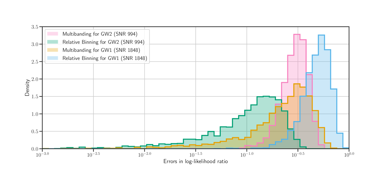
Figure 1: The histogram of errors in log-likelihood ratio obtained using 2500 samples drawn from the relative binning likelihood in a 40 km CE. For multibanding we use an accuracy_factor of 1 and enabled linear interpolation. For relative binning we set chi to 10 and epsilon to 0.1.

We evaluate the accuracy of the methods described in the previous section by selecting 2,500 downsampled points from the posterior distribution of GW1, observed in a 40 km CE. For each point, the exact log-likelihood ratio is calculated using GravitationalWaveTransientNextGeneration. As CE is the most sensitive detector considered in this study, the differences in log-likelihood ratios are expected to be even smaller for other detectors. The chosen signal has a high signal-to-noise ratio (SNR) and includes higher-order multipole moments, making it well-suited for this analysis. Additionally, we also validate the multibanding approximation. In both cases, the difference in log-likelihood ratios is found to be less than unity [46], as illustrated in Figure 1, confirming the robustness of our results. The errors in the log-likelihood ratio decrease as the signal-to-noise ratio (SNR) decreases, as expected. This reduction in likelihood errors is less pronounced for multibanding compared to relative binning, as the latter does not strictly account for frequency-dependent antenna response effects. The current scheme to determine frequency bins in relative binning is solely based on the Post-Newtonian inspiral phase, but it could be easily extended to incorporate the effects of Earth’s rotation and finite detector sizes, because their oscillatory scales in frequency domain can be easily estimated and frequency bins can be constructed so that those effects are accurately captured by the interpolation. The values of chi and epsilon are chosen such that the log-likelihood errors for the highest SNR signal remain below unity.

4.2 Inference using 1 Cosmic Explorer

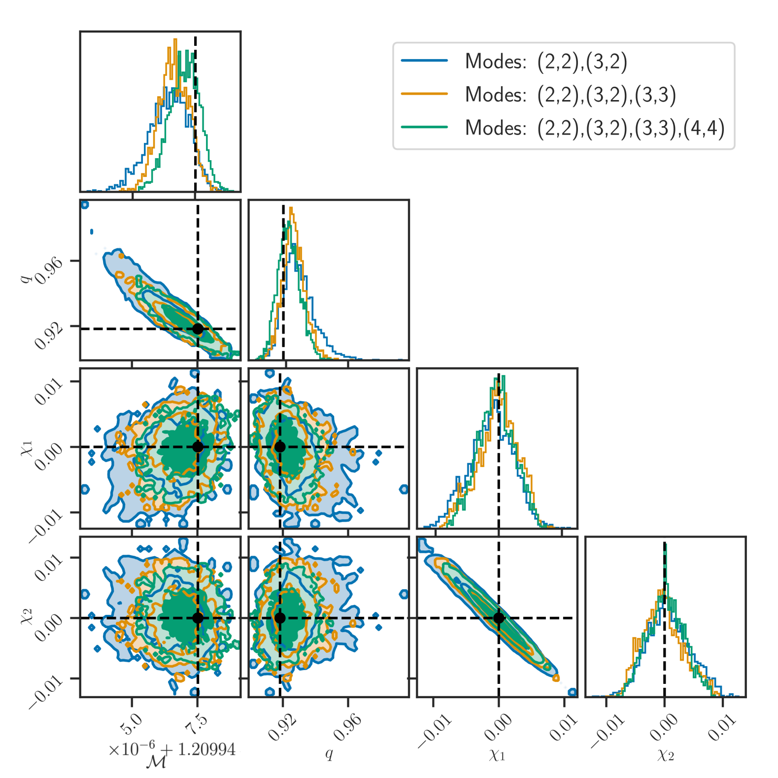
(a) GW1

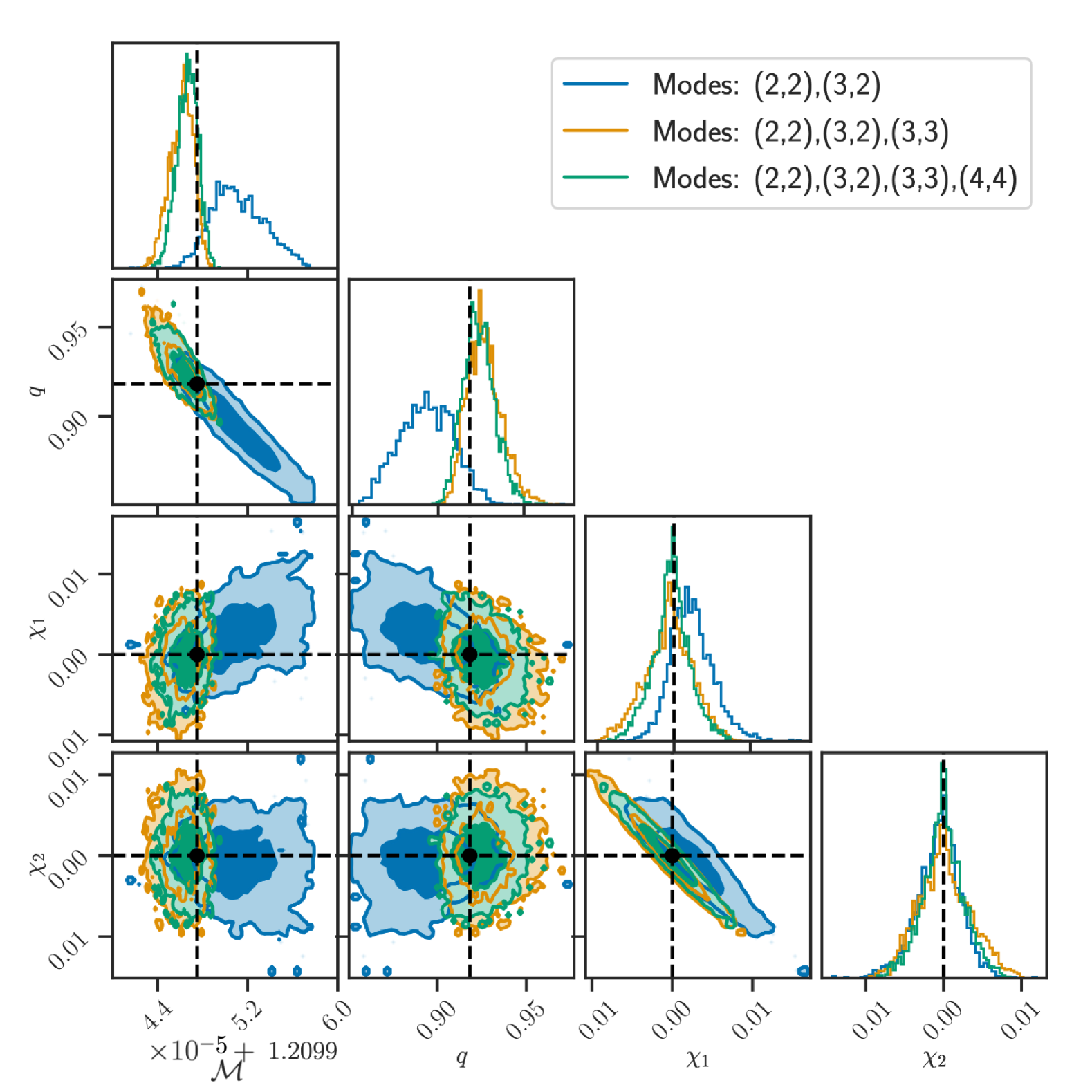
(b) GW2

Figure 2: Inferred posteriors of intrinsic parameters of GW1 and GW2 in a 40km CE. The green posteriors use all modes for analysis, the orange posterior ignore modes with m = 3 and the blue ones ignore m = 3 and m = 4 modes.

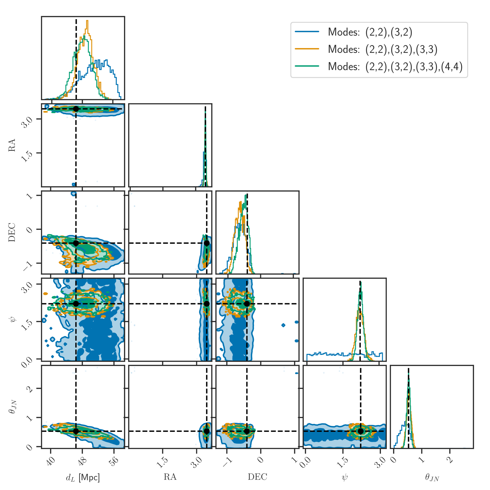
(a) GW1

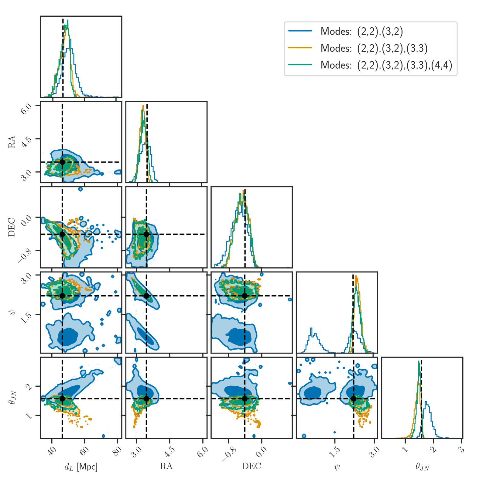
(b) GW2

Figure 3: Inferred posteriors of extrinsic parameters of GW1 and GW2 in one 40km CE. The green posteriors use all modes for analysis, the orange posterior ignore modes with m = 3 and the blue ones ignores m = 3 and m = 4 modes.

We start by looking at the posteriors of GW1 and GW2. For ease of visualization, we break the entire parameter space into intrinsic and extrinsic parameters.

4.2.1 Intrinsic Parameters

The inclusion of higher radiation modes for GW1 has a minimal impact on the intrinsic parameters due to the low signal-to-noise ratios (SNRs) associated with these modes (see Table 2). In the case of a perfectly face-on orientation ($\theta_{\rm JN}=0$), the spin-weighted spherical harmonics vanish for modes where m $\neq$ 2. Given that GW1 has a very small inclination, the effects of higher-order modes are significantly suppressed compared to GW2, as reflected in the posterior distributions.

4.2.2 Extrinsic Parameters

For the extrinsic parameters as well, the inclusion of higher modes has a greater impact on GW2 than on GW1. However, the posterior distribution of the polarization angle ($\psi$) presents an interesting case. When higher modes are not included in GW1, the recovered posterior follows the prior distribution (see 3(a)). In contrast, for GW2 without higher modes, the posterior exhibits a bimodal distribution (see 3(b)). A GW with its dominant l,m = 2,2 mode for the inspiral portion in a single detector can be written as,

$$h(t)=-\Big{(}\frac{G\mathcal{M}}{c^{2}D_{\text{eff}}}\Big{)}\Big{(}\frac{t_{0}-t}{5G\mathcal{M}/c^{3}}\Big{)}^{1/4}\cos\Big{[}2\phi(t-t_{0};\mathcal{M},q)+2\phi_{c}-\tan^{-1}\Big{(}\frac{F_{\times}}{F_{+}}\frac{2\cos\theta_{\textrm{JN}}}{1+\cos^{2}\theta_{\textrm{JN}}}\Big{)}\Big{]}$$ (12)

Here we only keep terms to the leading order in amplitude. The arrival time at the detector is $t$, while $t_{0}$ is the arrival time corresponding to the coalescence and

$$D_{\textrm{eff}}=D_{\textrm{L}}\Big{[}F_{+}^{2}\Big{(}\frac{1+\cos^{2}\theta_{\textrm{JN}}}{2}\Big{)}^{2}+F_{\times}^{2}\cos^{2}\theta_{\textrm{JN}}\Big{]}^{-1/2}$$ (13)

For small $\theta_{\texttt{JN}}$ we can write 14 as,

$$D_{\textrm{eff}}=D_{\textrm{L}}(1-\theta_{\textrm{JN}}^{2})^{-1/2}(F_{+}^{2}+F_{\times}^{2})^{-1/2}+\mathcal{O}(\theta_{\textrm{JN}}^{2})$$ (14)

If an interferometer has arms along the x and y axes and the source of the gravitational wave is at ($\theta,\phi$), then the beam-pattern function in the long wavelength limit is given by,

$$F_{+}\simeq-\frac{1}{2}(1+\cos^{2}\theta)\cos 2\phi\cos 2\psi-\cos\theta\sin 2\phi\sin 2\psi$$ (15)

and

$$F_{\times}\simeq\frac{1}{2}(1+\cos^{2}\theta)\cos 2\phi\sin 2\psi-\cos\theta\sin 2\phi\cos 2\psi$$ (16)

So,

$$F_{+}^{2}+F_{\times}^{2}\simeq\frac{1}{4}(1+\cos^{2}\theta)^{2}+\cos^{2}\phi$$ (17)

So the amplitude does not depend on the polarization angle to linear order in the inclination. This is because when the orbit of the binary is a circle in the sky, that circle is invariant under rotations on the plane of the sky. This is true even beyond the long-wavelength limit. The polarization angle enters equation 12 through the antenna responses and we have shown that the amplitude is independent of $\psi$. The only other place where $\psi$ comes in equation 12 is via the argument of the cosine term. For small $\theta_{\texttt{JN}}$, the term $\tan^{-1}\Big{(}\frac{F_{\times}}{F_{+}}\frac{2\cos\theta_{\textrm{JN}}}{1+\cos^{2}\theta_{\textrm{JN}}}\Big{)}$ reduces to $2\psi+f(\theta,\phi)$. So $\phi_{c}$ and $\psi$ are completely degenerate. Physically this is because the phase of the binary on the circle in the sky is degenerate with an overall rotation of that circle. For the m=2 mode only run, it is not possible to recover any information about $\psi$ unless and until we have higher modes or a network sensitive enough to detect quadratic terms in $\theta_{\rm JN}$. For a face-on system as discussed earlier, the spin-weighted spherical harmonics (${}_{-2}Y_{lm}$s) vanish except for m=$\pm$2. So without a m=3, m=4 $\phi_{c}$ and $\psi$ in the waveform’s phase would be degenerate .

For GW2, the same cannot be said as it is completely edge-on. In this limit $\tan^{-1}\Big{(}\frac{F_{\times}}{F_{+}}\frac{2\cos\theta_{\textrm{JN}}}{1+\cos^{2}\theta_{\textrm{JN}}}\Big{)}$ vanishes and the argument of the cosine term in equation 12 is independent of the geometric parameters and there exists no degeneracy with $\phi_{c}$. The amplitude depends only on $|F_{+}|$ which is invariant under the transformation $\psi\hookrightarrow\psi+\frac{\pi}{2}$ which is seen in 3(b). This is infact a more general degeneracy that exists in the polarization angle [47] when higher azimuthal modes are ignored.

4.3 Inference using a network of dectectors

As described earlier, we consider a network of:- CE and A1; CE and CE20; and CE, CE20, and A1. From our simulations, we can draw two conclusions.

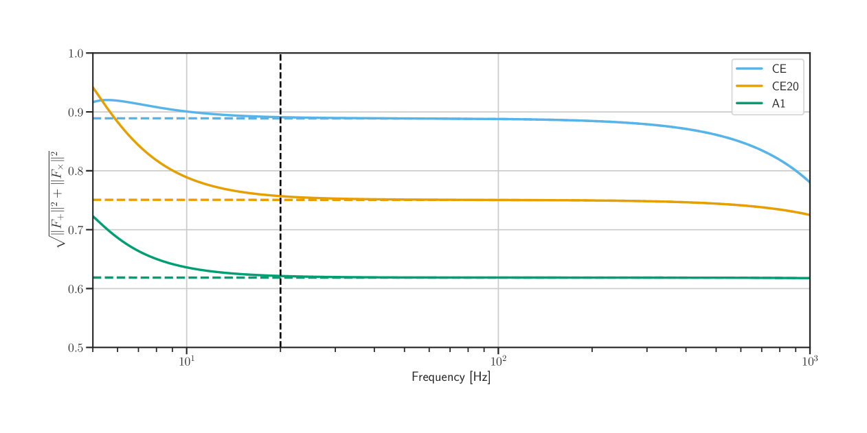
Figure 4: The antenna response as a function of frequency for GW1 and GW2 at the three detectors is analyzed. For CE and CE20, the response varies at low frequencies due to Earth’s rotation and at high frequencies due to detector-size effects. In the case of A1, the signal enters the band at 20 Hz, resulting in no frequency dependence at low frequencies. Additionally, due to the detector’s size, there is no effect at high frequencies.

• Intrinsic parameters: The network of CE and A1 performs better than only one CE, justifying operating one present-generation detector at design sensitivity with a next-generation detector. The CEA1 network is almost at par with the CECE20 and CECE20A1 networks for GW1 and GW2 as seen in 6(c) and 6(d). This is because both these events are of sufficiently high SNR and the phase can be measured accurately in A1. This is not expected to be true at lower SNRs. Also, we do not see much additional benefit from including higher modes of radiation for intrinsic parameters.

• Extrinsic parameters: Unlike the case for intrinsic parameters, a network of CE and CE20 is much better than a network of CE and A1 and is comparable to a network of CECE20A1. This is because for CE and CE20 Earth’s rotation has a significant effect on the amplitude (see figure 4), which is reflected in the recovered posteriors. Another interesting fact is that we see two peaks separated by an angle of $\pi/2$ for polarization angle in GW1 for a network of CECE20 and CECE20ET instead of recovering the prior as in the case of using 1 CE or in the CEA1. This is because the CECE20 and CECE20A1 are sensitive to terms of order $\mathcal{O}(\theta_{\rm JN}^{2})$. At this order, the amplitude is neither independent of $\psi$ nor is there a $\psi$, $\phi_{c}$ degeneracy. However the waveform is invariant under the transformation $\psi\hookrightarrow\psi+\frac{\pi}{2}$, which is a result of $|F_{+}|,|F_{\times}|$ and $\frac{F_{\times}}{F_{+}}$ being invariant under the same transformation.

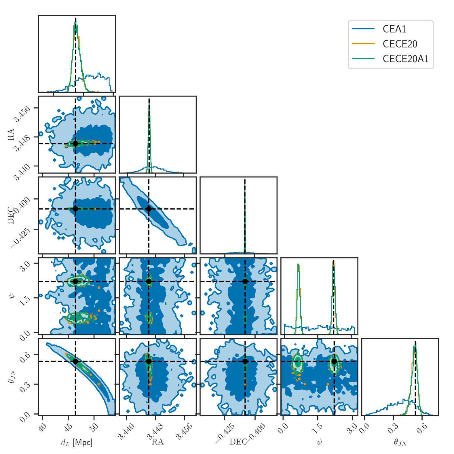
(a) Modes: (2,2),(3,2)

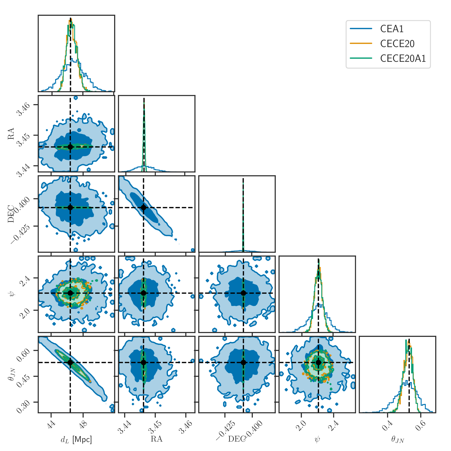
(b) Modes: (2,2), (3,2), (3,3), (4,4)

Figure 5: Inferred posteriors of extrinsic parameters of GW1 in networks comprising of:- a CE and A1 (blue); CE and CE20 (orange); and CE, CE20 and A1 (green).

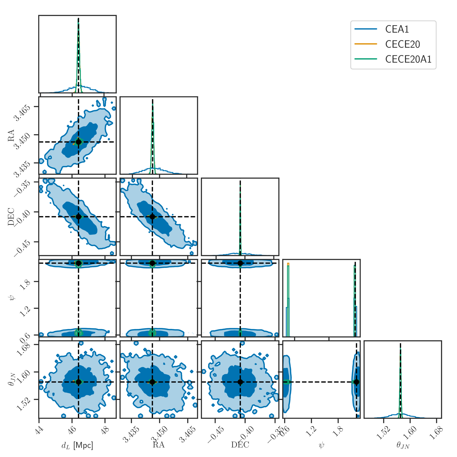
(a) Modes: (2,2), (3,2)

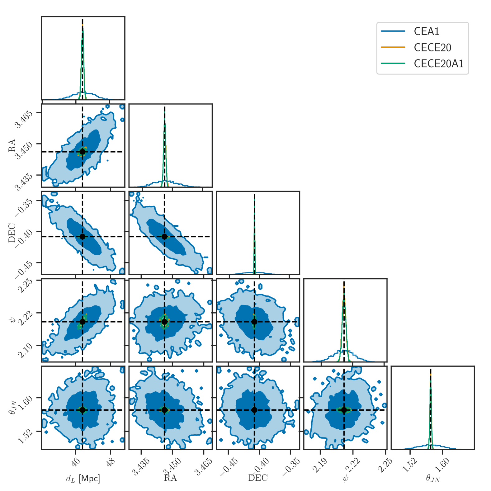
(b) Modes: (2,2), (3,2), (3,3), (4,4)

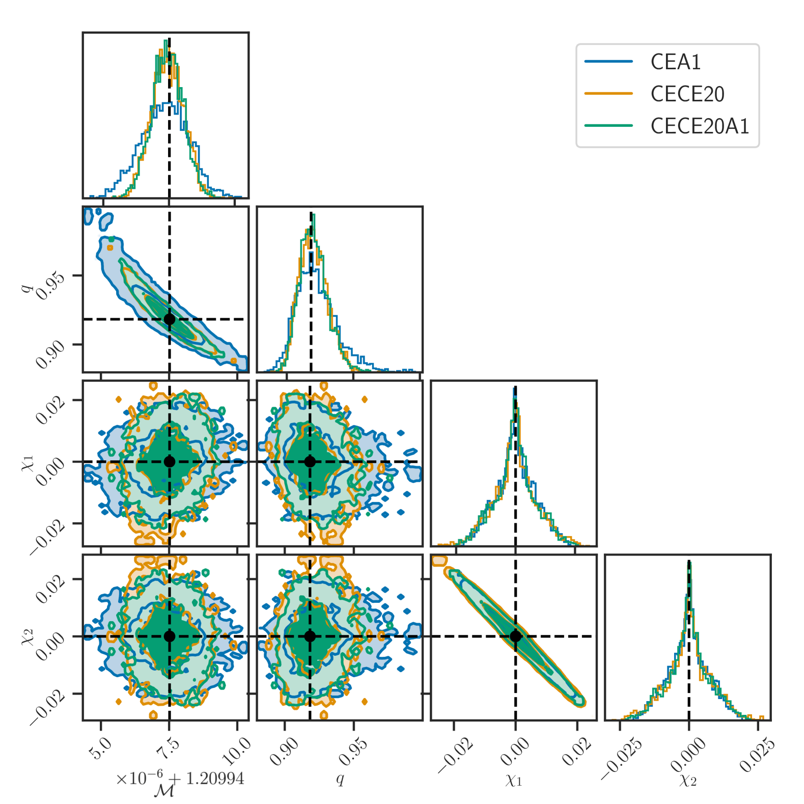
(c) Modes: (2,2), (3,2)

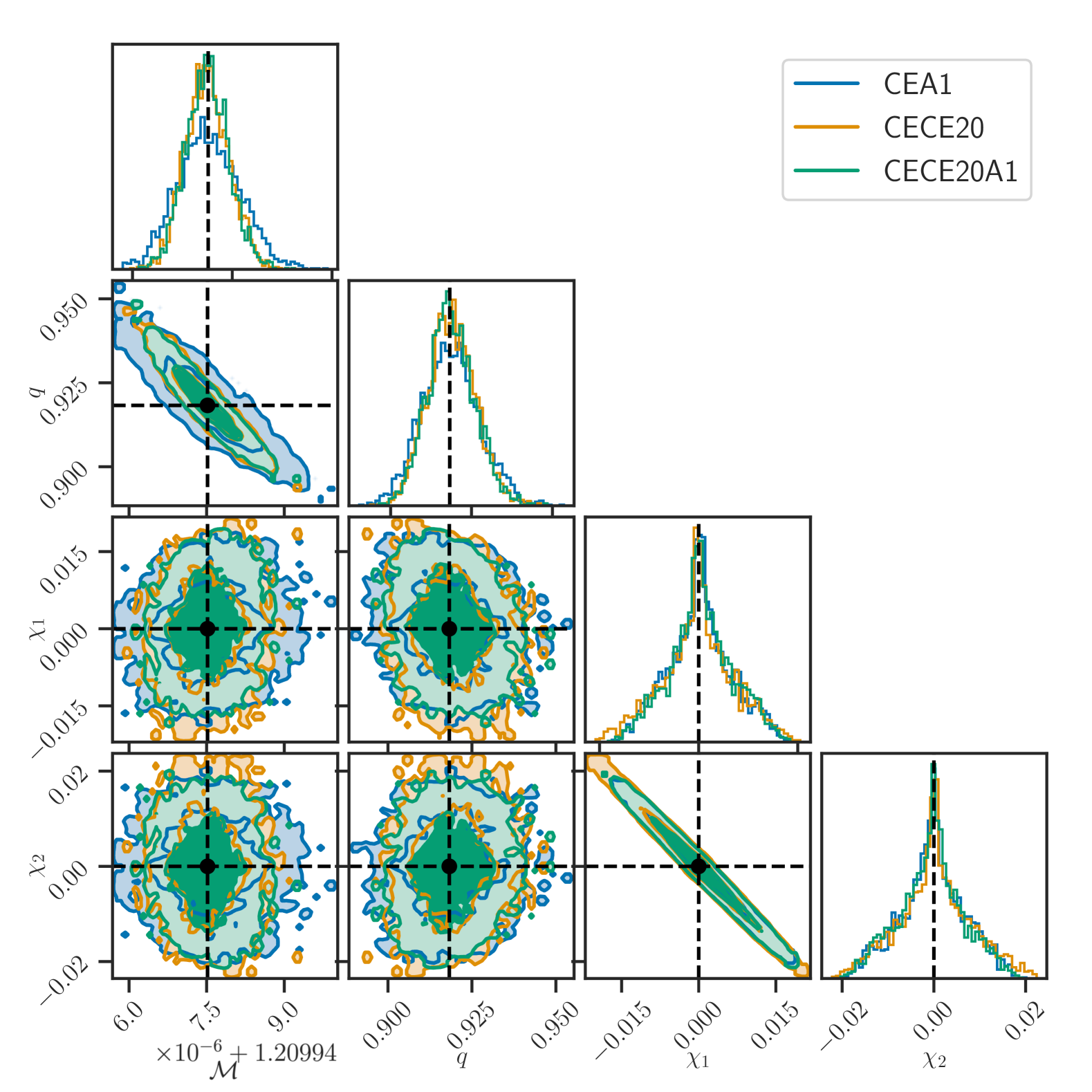
(d) Modes: (2,2), (3,2), (3,3), (4,4)

Figure 6: Inferred posteriors of extrinsic (top panel) and intrinsic (bottom panel) parameters of GW2 in networks comprising of: a CE and A1 (blue); CE and CE20 (orange); and CE, CE20 and A1 (green).

4.4 Localization

Long signals, detector size effects, higher modes, and multiple detectors help in localization. In the case of only one CE, we see a 26% improvement in the 90% sky area and a 60% improvement in 3D volume for GW1 after adding the (3,3) modes. The gain in localization with higher modes and 1 CE is much greater for GW2 as the higher modes of radiation are amplified because the source is edge-on. We see a 50% improvement in sky area and a 75% improvement in sky volume after the addition of the (3,3) mode. The detailed values are given in table 3. However, the gain due to higher modes is completely lost as we add another detector to form a baseline.

Modes used for inference	GW1				GW2
	90% Sky Area (in sq. deg.)		90% 3D Sky Volume (Mpc3)		90% Sky Area (in sq. deg.)		90 % 3D Sky Volume ($Mpc^{3}$)
	CE	CEA1	CE	CEA1	CE	CEA1	CE	CEA1
(2,2), (3,2)	234	<0.5	2668	<3	1677	<3	16235	<3
(2,2), (3,2), (3,3)	173	<0.5	1092	<2	829	<3	4091	<3
(2,2), (3,2), (3,3) & (4,4)	149	<0.5	744	<2	985	<3	2778	<3

Table 3: The 90% sky areas and 90% 3d sky volumes for GW1 and GW2 in one 40km CE and a network of CE and A1. Note the injections have all modes of radiation.

5 Conclusions

In this paper, we have developed the tools necessary to generate gravitational waveforms for next-generation detectors, incorporating effects due Earth’s rotation, detector size, and higher-order modes, all within the Bilby framework. To handle these waveforms, we implemented four new likelihood classes: one exact and three approximations.

Using the IMRPhenomXPHM waveform family, we simulated gravitational wave signals for next-generation detectors. As BNS waveforms with higher-order modes are not yet available in the literature, we use BBH waveforms which essentially sets the tidal parameters to zero for these simulations. However, our framework supports the inclusion of tidal effects without additional modifications. For PE, we adopted aligned spin priors and used the computational efficient mode-by-mode relative binning likelihood to explore the ten-dimensional posterior space. The fiducial waveform was matched to the injected waveform for simplicity, recognizing that this assumption is infeasible in practical applications. However, this approach does not impact the primary goal of this work, which is to evaluate measurement accuracies in next-generation detectors rather than to develop PE algorithms for future detector operations. These PE runs, parallelized across 16 threads on a computing cluster, required approximately one day of wall-clock time. Additional computational optimizations, such as cython-based implementations of beam-pattern functions, could further enhance efficiency, as suggested in the literature [48].

We conducted illustrative parameter estimation for two GW170817-like sources: one nearly face-on and the other edge-on. Injections included all modes, while PE runs were performed with and without the subdominant modes. For a single 40 km Cosmic Explorer (CE) detector, the inclusion of HMs improved parameter recovery. However, this advantage diminished in a network configuration of detectors. Regardless, HMs proved essential for accurately measuring the polarization angle and phase, avoiding degeneracies in both cases.

The posteriors obtained by incorporating all modes of radiation appear fairly Gaussian and lack any multimodalities. Therefore, we anticipate that the Fisher formalism would provide an accurate approximation. However, this remains to be explored in future work.

The accuracy controlling free parameters of our approximations were calibrated to ensure that errors remain smaller than the statistical uncertainties in PE for SNRs around 1000. For lower SNRs, where statistical uncertainties are naturally larger, the approximation parameters can be adjusted to reduce computational costs further. Additionally, at lower SNRs, the sampling process is easier and quicker. Our current methodology assumes the presence of a single signal in the data; extensions will be necessary to address overlapping signals expected in low-SNR regimes.

We employed the displacement PSD, scaled by the detector length, to ensure that the noise PSD remains free from high-frequency corrections. While this paper primarily focuses on methods for studying CBCs in next-generation detectors, the proposed framework is adaptable to minor variations in PSDs or detector locations, which are yet to be finalized.

$Software:$ Analysis in this paper made use of Bilby [33] with new features available in [49], LALSuitev7.2.4 [50], NumPyv1.26.4 [51], SciPyv1.13.1 [52], Astropyv6.1.1 [53, 54] and Matplotlibv3.7.5 [55].

$Data\leavevmode\nobreak\ and\leavevmode\nobreak\ code\leavevmode\nobreak\ availability:$ The codes for this project are hosted in https://git.ligo.org/pratyusava.baral/ce_hm_paper.

6 Acknowledgement

This work carries LIGO document number P2500078. The authors are thankful to Anson Chen for providing useful insights during internal LIGO review. This work was supported partially by the National Science Foundation (NSF) awards PHY-2207728 and PHY-2110576 and partially by Wisconsin Space Grant Consortium Awards RFP23_2-0 and RFP24_3-0. SM acknowledges support from JSPS Grant-in-Aid for Transformative Research Areas (A) No. 23H04891 and No. 23H04893. The authors are grateful for computational resources provided by the LIGO Laboratory and those provided by Cardiff University, and funded by an STFC grant supporting UK Involvement in the Operation of Advanced LIGO. PB is also grateful to the XG Mock Data Challenge workshop at Penn State University in May 2024.

References

- [1] The LIGO Scientific Collaboration and the Virgo Collaboration. GWTC-3: Compact binary coalescences observed by ligo and virgo during the second part of the third observing run, 2021. URL: https://arxiv.org/abs/2111.03606, doi:10.48550/arxiv.2111.03606.
- [2] Alexander H. Nitz, Sumit Kumar, Yi-Fan Wang, Shilpa Kastha, Shichao Wu, Marlin Schäfer, Rahul Dhurkunde, and Collin D. Capano. 4-OGC: Catalog of gravitational waves from compact-binary mergers, 2021. URL: https://arxiv.org/abs/2112.06878, doi:10.48550/arxiv.2112.06878.
- [3] The LIGO Scientific Collaboration and the Virgo Collaboration. GW170817: Observation of gravitational waves from a binary neutron star inspiral. Phys. Rev. Lett., 119:161101, Oct 2017. URL: https://link.aps.org/doi/10.1103/PhysRevLett.119.161101, doi:10.1103/PhysRevLett.119.161101.
- [4] The LIGO Scientific Collaboration, the Virgo Collaboration, and the KAGRA Collaboration. Gw190425: Observation of a compact binary coalescence with total mass 3̃-4 . The Astrophysical Journal Letters, 892(1):L3, mar 2020. URL: https://dx.doi.org/10.3847/2041-8213/ab75f5, doi:10.3847/2041-8213/ab75f5.
- [5] The LIGO Scientific Collaboration, the Virgo Collaboration, and the KAGRA Collaboration. Observation of gravitational waves from two neutron starblack hole coalescences. The Astrophysical Journal Letters, 915(1):L5, jun 2021. URL: https://dx.doi.org/10.3847/2041-8213/ac082e, doi:10.3847/2041-8213/ac082e.
- [6] The LIGO Scientific Collaboration and the Virgo Collaboration. Advanced ligo. Classical and Quantum Gravity, 32(7):074001, mar 2015. URL: https://dx.doi.org/10.1088/0264-9381/32/7/074001, doi:10.1088/0264-9381/32/7/074001.
- [7] The LIGO Scientific Collaboration and the Virgo Collaboration. Advanced virgo: a second-generation interferometric gravitational wave detector. Classical and Quantum Gravity, 32(2):024001, dec 2014. URL: https://dx.doi.org/10.1088/0264-9381/32/2/024001, doi:10.1088/0264-9381/32/2/024001.
- [8] The LIGO Scientific Collaboration, the Virgo Collaboration, and the KAGRA Collaboration. Overview of KAGRA : KAGRA science, 2020. URL: https://arxiv.org/abs/2008.02921, doi:10.48550/arxiv.2008.02921.
- [9] LIGO Scientific Collaboration and Virgo Collaboration. Gravitational-wave candidate event database (GraceDB). https://gracedb.ligo.org/, 2024. Accessed: 2024-11-16.
- [10] The LIGO Scientific Collaboration, the Virgo Collaboration, and the KAGRA Collaboration. Constraints on the cosmic expansion history from gwtc-3, 2021. URL: https://arxiv.org/abs/2111.03604, doi:10.48550/ARXIV.2111.03604.
- [11] The LIGO Scientific Collaboration, the Virgo Collaboration, and the KAGRA Collaboration. The population of merging compact binaries inferred using gravitational waves through gwtc-3, 2021. URL: https://arxiv.org/abs/2111.03634, doi:10.48550/arxiv.2111.03634.
- [12] The LIGO Scientific Collaboration, the Virgo Collaboration, and the KAGRA Collaboration. Tests of general relativity with gwtc-3, 2021. URL: https://arxiv.org/abs/2112.06861, doi:10.48550/arxiv.2112.06861.
- [13] David Reitze et al. Cosmic Explorer: The U.S. Contribution to Gravitational-Wave Astronomy beyond LIGO. Bulletin of the AAS, 51(7), sep 30 2019. https://baas.aas.org/pub/2020n7i035.
- [14] M Punturo et al. The einstein telescope: a third-generation gravitational wave observatory. Classical and Quantum Gravity, 27(19):194002, sep 2010. URL: https://dx.doi.org/10.1088/0264-9381/27/19/194002, doi:10.1088/0264-9381/27/19/194002.
- [15] Michele Maggiore et al. Science case for the einstein telescope. Journal of Cosmology and Astroparticle Physics, 2020(03):050, mar 2020. URL: https://dx.doi.org/10.1088/1475-7516/2020/03/050, doi:10.1088/1475-7516/2020/03/050.
- [16] Matthew Evans et al. Cosmic explorer: A submission to the nsf mpsac nggw subcommittee, 2023. URL: https://arxiv.org/abs/2306.13745, arXiv:2306.13745.
- [17] Marica Branchesi et al. Science with the einstein telescope: a comparison of different designs. Journal of Cosmology and Astroparticle Physics, 2023(07):068, jul 2023. URL: https://dx.doi.org/10.1088/1475-7516/2023/07/068, doi:10.1088/1475-7516/2023/07/068.
- [18] Vishal Baibhav, Emanuele Berti, Davide Gerosa, Michela Mapelli, Nicola Giacobbo, Yann Bouffanais, and Ugo N. Di Carlo. Gravitational-wave detection rates for compact binaries formed in isolation: Ligo/virgo o3 and beyond. Phys. Rev. D, 100:064060, Sep 2019. URL: https://link.aps.org/doi/10.1103/PhysRevD.100.064060, doi:10.1103/PhysRevD.100.064060.
- [19] M Rakhmanov, J D Romano, and J T Whelan. High-frequency corrections to the detector response and their effect on searches for gravitational waves. Classical and Quantum Gravity, 25(18):184017, sep 2008. URL: https://dx.doi.org/10.1088/0264-9381/25/18/184017, doi:10.1088/0264-9381/25/18/184017.
- [20] M Rakhmanov. On the round-trip time for a photon propagating in the field of a plane gravitational wave. Classical and Quantum Gravity, 26(15):155010, jul 2009. URL: https://dx.doi.org/10.1088/0264-9381/26/15/155010, doi:10.1088/0264-9381/26/15/155010.
- [21] Pratyusava Baral, Soichiro Morisaki, Ignacio Magaña Hernandez, and Jolien Creighton. Localization of binary neutron star mergers with a single cosmic explorer. Phys. Rev. D, 108:043010, Aug 2023. URL: https://link.aps.org/doi/10.1103/PhysRevD.108.043010, doi:10.1103/PhysRevD.108.043010.
- [22] Man Leong Chan, Chris Messenger, Ik Siong Heng, and Martin Hendry. Binary neutron star mergers and third generation detectors: Localization and early warning. Phys. Rev. D, 97:123014, Jun 2018. URL: https://link.aps.org/doi/10.1103/PhysRevD.97.123014, doi:10.1103/PhysRevD.97.123014.
- [23] Wen Zhao and Linqing Wen. Localization accuracy of compact binary coalescences detected by the third-generation gravitational-wave detectors and implication for cosmology. Phys. Rev. D, 97:064031, Mar 2018. URL: https://link.aps.org/doi/10.1103/PhysRevD.97.064031, doi:10.1103/PhysRevD.97.064031.
- [24] Shang-Jie Jin, Dong-Ze He, Yidong Xu, Jing-Fei Zhang, and Xin Zhang. Forecast for cosmological parameter estimation with gravitational-wave standard siren observation from the cosmic explorer. Journal of Cosmology and Astroparticle Physics, 2020(03):051, mar 2020. URL: https://dx.doi.org/10.1088/1475-7516/2020/03/051, doi:10.1088/1475-7516/2020/03/051.
- [25] Luca Reali, Roberto Cotesta, Andrea Antonelli, Konstantinos Kritos, Vladimir Strokov, and Emanuele Berti. Intermediate-mass black hole binary parameter estimation with next-generation ground-based detector networks. Phys. Rev. D, 110:103002, Nov 2024. URL: https://link.aps.org/doi/10.1103/PhysRevD.110.103002, doi:10.1103/PhysRevD.110.103002.
- [26] A. Makai Baker, Paul D. Lasky, Eric Thrane, and Jacob Golomb. Significant challenges for astrophysical inference with next-generation gravitational-wave observatories, 2025. URL: https://arxiv.org/abs/2503.04073, arXiv:2503.04073.
- [27] Alexander H. Nitz and Tito Dal Canton. Pre-merger localization of compact-binary mergers with third-generation observatories. The Astrophysical Journal Letters, 917(2):L27, August 2021. doi:10.3847/2041-8213/ac1a75.
- [28] Barak Zackay, Liang Dai, and Tejaswi Venumadhav. Relative binning and fast likelihood evaluation for gravitational wave parameter estimation, 2018. URL: https://arxiv.org/abs/1806.08792, arXiv:1806.08792.
- [29] Rory Smith, Ssohrab Borhanian, Bangalore Sathyaprakash, Francisco Hernandez Vivanco, Scott E. Field, Paul Lasky, Ilya Mandel, Soichiro Morisaki, David Ottaway, Bram J. J. Slagmolen, Eric Thrane, Daniel Töyrä, and Salvatore Vitale. Bayesian inference for gravitational waves from binary neutron star mergers in third generation observatories. Phys. Rev. Lett., 127:081102, Aug 2021. URL: https://link.aps.org/doi/10.1103/PhysRevLett.127.081102, doi:10.1103/PhysRevLett.127.081102.
- [30] Soichiro Morisaki. Accelerating parameter estimation of gravitational waves from compact binary coalescence using adaptive frequency resolutions. Phys. Rev. D, 104:044062, Aug 2021. URL: https://link.aps.org/doi/10.1103/PhysRevD.104.044062, doi:10.1103/PhysRevD.104.044062.
- [31] Anna Puecher, Anuradha Samajdar, and Tim Dietrich. Measuring tidal effects with the einstein telescope: A design study. Phys. Rev. D, 108:023018, Jul 2023. URL: https://link.aps.org/doi/10.1103/PhysRevD.108.023018, doi:10.1103/PhysRevD.108.023018.
- [32] Sylvain Marsat, John G. Baker, and Tito Dal Canton. Exploring the bayesian parameter estimation of binary black holes with lisa. Phys. Rev. D, 103:083011, Apr 2021. URL: https://link.aps.org/doi/10.1103/PhysRevD.103.083011, doi:10.1103/PhysRevD.103.083011.
- [33] Gregory Ashton et al. Bilby: A user-friendly bayesian inference library for gravitational-wave astronomy. apjs, 241(2):27, April 2019. arXiv:1811.02042, doi:10.3847/1538-4365/ab06fc.
- [34] Jolien D. E. Creighton and Warren G. Anderson. Gravitational-Wave Physics and Astronomy: An Introduction to Theory, Experiment and Data Analysis. Wiley-VCH, oct 2011.
- [35] Reed Essick, Salvatore Vitale, and Matthew Evans. Frequency-dependent responses in third generation gravitational-wave detectors. Phys. Rev. D, 96:084004, Oct 2017. URL: https://link.aps.org/doi/10.1103/PhysRevD.96.084004, doi:10.1103/PhysRevD.96.084004.
- [36] Eric Poisson and Clifford M. Will. Gravitational waves from inspiraling compact binaries: Parameter estimation using second-post-newtonian waveforms. Phys. Rev. D, 52:848–855, Jul 1995. URL: https://link.aps.org/doi/10.1103/PhysRevD.52.848, doi:10.1103/PhysRevD.52.848.
- [37] Juan CalderĂłn Bustillo, Alejandro BohĂŠ, Sascha Husa, Alicia M. Sintes, Mark Hannam, and Michael PĂźrrer. Comparison of subdominant gravitational wave harmonics between post-newtonian and numerical relativity calculations and construction of multi-mode hybrids, 2015. URL: https://arxiv.org/abs/1501.00918, arXiv:1501.00918.
- [38] Cecilio García-Quirós, Marta Colleoni, Sascha Husa, Héctor Estellés, Geraint Pratten, Antoni Ramos-Buades, Maite Mateu-Lucena, and Rafel Jaume. Multimode frequency-domain model for the gravitational wave signal from nonprecessing black-hole binaries. Phys. Rev. D, 102:064002, Sep 2020. URL: https://link.aps.org/doi/10.1103/PhysRevD.102.064002, doi:10.1103/PhysRevD.102.064002.
- [39] Barak Zackay, Liang Dai, and Tejaswi Venumadhav. Relative Binning and Fast Likelihood Evaluation for Gravitational Wave Parameter Estimation. 6 2018. arXiv:1806.08792.
- [40] Kruthi Krishna, Aditya Vijaykumar, Apratim Ganguly, Colm Talbot, Sylvia Biscoveanu, Richard N. George, Natalie Williams, and Aaron Zimmerman. Accelerated parameter estimation in Bilby with relative binning. 12 2023. arXiv:2312.06009.
- [41] Nathaniel Leslie, Liang Dai, and Geraint Pratten. Mode-by-mode relative binning: Fast likelihood estimation for gravitational waveforms with spin-orbit precession and multiple harmonics. Phys. Rev. D, 104(12):123030, 2021. arXiv:2109.09872, doi:10.1103/PhysRevD.104.123030.
- [42] Ish Gupta. Inferring Small Neutron Star Spins with Neutron Star–Black Hole Mergers. Astrophys. J., 970(1):12, 2024. arXiv:2402.07075, doi:10.3847/1538-4357/ad49a0.
- [43] Varun Srivastava, Derek Davis, Kevin Kuns, Philippe Landry, Stefan Ballmer, Matthew Evans, Evan D. Hall, Jocelyn Read, and B. S. Sathyaprakash. Science-driven tunable design of cosmic explorer detectors. The Astrophysical Journal, 931(1):22, may 2022. URL: https://dx.doi.org/10.3847/1538-4357/ac5f04, doi:10.3847/1538-4357/ac5f04.
- [44] Geraint Pratten, Cecilio García-Quirós, Marta Colleoni, Antoni Ramos-Buades, Héctor Estellés, Maite Mateu-Lucena, Rafel Jaume, Maria Haney, David Keitel, Jonathan E. Thompson, and Sascha Husa. Computationally efficient models for the dominant and subdominant harmonic modes of precessing binary black holes. Phys. Rev. D, 103:104056, May 2021. URL: https://link.aps.org/doi/10.1103/PhysRevD.103.104056, doi:10.1103/PhysRevD.103.104056.
- [45] Chris Pankow, Katerina Chatziioannou, Eve A. Chase, Tyson B. Littenberg, Matthew Evans, Jessica McIver, Neil J. Cornish, Carl-Johan Haster, Jonah Kanner, Vivien Raymond, Salvatore Vitale, and Aaron Zimmerman. Mitigation of the instrumental noise transient in gravitational-wave data surrounding gw170817. Phys. Rev. D, 98:084016, Oct 2018. URL: https://link.aps.org/doi/10.1103/PhysRevD.98.084016, doi:10.1103/PhysRevD.98.084016.
- [46] Serena Vinciguerra, John Veitch, and Ilya Mandel. Accelerating gravitational wave parameter estimation with multi-band template interpolation. Classical and Quantum Gravity, 34(11):115006, may 2017. URL: https://dx.doi.org/10.1088/1361-6382/aa6d44, doi:10.1088/1361-6382/aa6d44.
- [47] Javier Roulet, Seth Olsen, Jonathan Mushkin, Tousif Islam, Tejaswi Venumadhav, Barak Zackay, and Matias Zaldarriaga. Removing degeneracy and multimodality in gravitational wave source parameters. Phys. Rev. D, 106:123015, Dec 2022. URL: https://link.aps.org/doi/10.1103/PhysRevD.106.123015, doi:10.1103/PhysRevD.106.123015.
- [48] Anson Chen and Nathan K Johnson-McDaniel. A fast frequency-domain expression for the time-dependent detector response of ground-based gravitational-wave detectors to compact binary signals, 2024. URL: https://arxiv.org/abs/2407.15732, arXiv:2407.15732.
- [49] Pratyusava Baral. bilby_xg: Frequency dependent antenna response with higher modes. https://git.ligo.org/pratyusava.baral/bilby-x-g/-/tree/freq_dep_antenna_response_HM. Accessed: 2025-03-07.
- [50] LIGO Scientific Collaboration. LIGO Algorithm Library - LALSuite. free software (GPL), 2018. doi:10.7935/GT1W-FZ16.
- [51] Charles R. Harris et al. Array programming with NumPy. Nature, 585(7825):357–362, September 2020. doi:10.1038/s41586-020-2649-2.
- [52] Pauli Virtanen et al. SciPy 1.0: fundamental algorithms for scientific computing in python. Nature Methods, 17(3):261–272, February 2020. doi:10.1038/s41592-019-0686-2.
- [53] Thomas P. Robitaille et al. Astropy: A community python package for astronomy. Astronomy & Astrophysics, 558:A33, September 2013. doi:10.1051/0004-6361/201322068.
- [54] A. M. Price-Whelan et al. The astropy project: Building an open-science project and status of the v2.0 core package. The Astronomical Journal, 156(3):123, August 2018. doi:10.3847/1538-3881/aabc4f.
- [55] John D. Hunter. Matplotlib: A 2d graphics environment. Computing in Science & Engineering, 9(3):90–95, 2007. doi:10.1109/MCSE.2007.55.