Extension of Sequence of Physical Processes framework relating the second Piola-Kirchhoff stress tensor to the Green-Lagrange strain tensor

Abstract

An extension of the Sequence of Physical Processes using geometrical corrections of the Piola-Kirchhoff stress tensor and the Green-Lagrange strain tensor is addressed. More precisely, the usual Sequence of Physical Processes omits some geometrical non linearities that appear when the deformation becomes large. With this extension, geometrical corrections are added and let the opportunity to study rheological non linearities. Application on two famous classical viscoelastic models, namely the linear Maxwell model and the linear Kelvin-Voigt model, helps to understand how some complex behaviours may be rationalised to better understand the behaviours after some corrections.

I Introduction

General rheological models started to be created when continuum mechanics needed traditional ones to close their equations [1, 2, 3, 4]. In fact, rheology as a discipline started years before the complete formalisation of continuum mechanics and relied mainly on empirical observations[5, 6, 7, 8, 9, 10, 11, 12]. At the end of the twentieth century, studies began to rationalise the construction of rheological models to comply with thermodynamics for instance[13, 4]. These framework were very important to properly account for physical phenomena happening in certain materials. Besides, most of the usual rheological models were first built in small deformations framework to avoid, at first, non linearities. However, recent studies[14, 15, 16] have demonstrated the interest of large deformations study to properly understand the behaviour of some materials. The proper theoretical interpretation must take into account some geometrical effect when materials evolve due to forces, displacement or other solicitations. For instance, in continuum mechanics, the Eulerian framework and the Lagrangian framework helps to distinguish between the current configuration and the initial configuration in terms of strains or in terms of stresses[17, 18]. Even if this type of consideration may be found in certain studies, it is not the case for all rheological frameworks.

In this paper, the Sequence of Physical Processes designed by [19, 20, 21, 22, 23] is analysed in the perpective of large deformations. The original development is indeed made in a linear way without accounting for geometrical corrections at large deformations. The extension of this framework will be addressed through the use of the second Piola-Kirchhoff stress tensor and the Green-Lagrange strain tensor, which are thermodynamics conjugates, and allow the analysis to come back to the initial configuration.

In section˜II, the theoretical development of the extended framework will be presented. Then, in section˜III, two application cases are studied with the two classical linear viscoelastic models, namely, the Maxwell model[10] and the Kelvin-Voigt model[11, 12]. Afterwards, some remarks and warning are highlighted in section˜IV. Finally, some conclusions are drawn in section˜V.

II Derivation of the extension

To recall the usual sequence of Physical Processes presented in [19, 20, 21, 22, 23], it is possible via the Frénet-Serret frame to find a transient viscoelastic modulus $G_{t}$ relating the shear stress $\sigma$ to the shear strain $\varepsilon$ and the shear strain rate $\dot{\varepsilon}$. The whole demonstration relies on the fact that there is a linear relationship in the frequency domain between the stress tensor $\bm{\sigma}$ and the strain tensor $\bm{\varepsilon}$ of the form $\bm{\sigma}=\mathbb{C}\bm{\varepsilon}$ with $\mathbb{C}$ a fourth order tensor gathering the material properties. Acknowledging the power of such tools, it is interesting to question the relevance of these last assumptions. For instance, when increasing the amplitude of the oscillation of the shear strain, rheological non-linearities may appear, as well as geometrical non-linearities. Then, it may be interesting to decorrelate both previous effects to study only the rheological non-linearities. Such a framework exists in continuum mechanics and is related to hyperelastic materials. Precisely, the Cauchy stress tensor $\bm{\sigma}$ and the linear strain tensor $\bm{\varepsilon}$ are properly defined in the deformed configuration of a material. When the latter undergoes large deformation, the deformed configuration becomes pretty different from the reference configuration. Therefore, it is possible to create two quantities that are defined in the reference configuration and allow to connect stresses and deformations: namely, the second Piola-Kirchhoff stress tensor $\bm{S}$ and the Green-Lagrange strain tensor $\bm{e}$. To recall the construction of such quantities, the transformation from the reference configuration to the deformed configuration is determined by the deformation gradient of the displacement $\bm{F}$. Using some differential transformation of distances, areas and volumes, the deformations from the reference configuration are properly measured by the Green-Lagrange strain tensor defined by

$$\bm{e}=\frac{1}{2}\left(\bm{F}^{T}\bm{F}-\bm{I}\right)$$ (1)

with $\cdot^{T}$ the transpose of a tensor and $\bm{I}$ the identity tensor. Simultaneously, the forces in the deformed configuration acting on areas in the deformed configuration are given by the Cauchy stress tensor $\bm{\sigma}$ and can be pulled back to forces in the reference configuration acting on areas in the reference configuration through the second Piola-Kirchhoff stress tensor $\bm{S}$ defined by

$$\bm{S}=J\bm{F}^{-1}\bm{\sigma}\bm{F}^{-T}$$ (2)

with $J=\det\left(\bm{F}\right)$. In the case of small deformation, $J\approx 1$, $\bm{F}\approx\bm{I}+\bm{\nabla u}$ with $\bm{u}$ the displacement, thus the Green-Lagrange strain tensor $\bm{e}$ is equal to the usual linear strain tensor $\bm{\varepsilon}$ and the second Piola-Kirchhoff stress tensor $\bm{S}$ is equal to the usual Cauchy stress tensor $\bm{\sigma}$. However, in the case of large transformations, the Green-Lagrange strain tensor and the second Piola-Kirchhoff stress tensor account for rotations and large deformations. Relating to the hyperelastic materials framework, it can be demonstrated that the second Piola-Kirchhoff stress tensor and the Green-Lagrange strain tensor are energy conjuguates meaning that a rheological law involving an expression of $\bm{S}$ as a function of $\bm{e}$ or its derivatives is objective and properly defined. In addition, it can be demonstrated[25] that the mechanical energy per unit volume in the reference configuration due to the material is equal to $\bm{S}:\dot{\bm{e}}$ with $:$ the double contracted product and $\dot{\left(\cdot\right)}$ the time derivative. Therefore, in the Fourier domain, it is straightforward to consider, as a first approach, that it exists a complex fourth order tensor $\mathbb{H}$ reading $\bm{S}=\mathbb{H}\bm{e}$.

Now with these previous remarks, it is possible to extend the usual Sequence of Physical Processes method. In this framework, an imposed oscillatory shear strain $\varepsilon=\varepsilon_{0}\sin\left(\omega t\right)$ with $\varepsilon_{0}$ the shear strain amplitude and $\omega$ the pulsation drives the deformation of the material. Assuming that the shear strain is imposed in the $xy$ plane in cartesian coordinates and using the definition of the deformation gradient $\bm{F}$ and eqs.˜1 and 2, one gets

$$\bm{F} =\bm{I}+\varepsilon\bm{e}_{x}\otimes\bm{e}_{y}$$ (3)

$$\bm{S} =\bm{\sigma}-\varepsilon\begin{pmatrix}2\sigma_{xy}-\varepsilon\sigma_{yy}&\sigma_{yy}&\sigma_{yz}\\ \sigma_{yy}&0&0\\ \sigma_{yz}&0&0\end{pmatrix}$$ (4)

$$2\bm{e} =\varepsilon\left(\bm{e}_{x}\otimes\bm{e}_{y}+\bm{e}_{y}\otimes\bm{e}_{x}\right)+\varepsilon^{2}\bm{e}_{y}\otimes\bm{e}_{y}.$$ (5)

Hence, while in the usual Sequence of Physical Processes framework, one can write $\sigma=G^{\prime}\varepsilon+G^{\prime\prime}\dot{\varepsilon}/\omega$ with $\dot{\varepsilon}$ the shear strain rate, here one gets

$$S=G^{\prime}\varepsilon+G^{\prime\prime}\frac{\dot{\varepsilon}}{\omega}+H^{\prime}\varepsilon^{2}+H^{\prime\prime}\frac{2\varepsilon\dot{\varepsilon}}{\omega}$$ (6)

with $S$ any components of $\bm{S}$ and $G^{\prime},G^{\prime\prime},H^{\prime},H^{\prime\prime}$ the various moduli of the rheological law which are going to be extended in instantaneous values. To build these instantaneous values, instead of considering a three dimensions space with a position vector $\bm{x}=\left(\varepsilon,\dot{\varepsilon}/\omega,\sigma\right)$, let us consider a position vector $\bm{x}=\left(\varepsilon,\dot{\varepsilon}/\omega,\varepsilon^{2},2\dot{\varepsilon}\varepsilon/\omega,S\right)$ and let us try to build a Frénet-Serret apparatus on this five dimensions space. Following the Gram-Schmidt procedure for the vector family $\left(\mathrm{d}_{t}^{j}\bm{x}\right)_{j\in\left\llbracket 1,5\right\rrbracket}$, we define a family $\left(\bm{e}_{i}\right)_{i\in\left\llbracket 1,5\right\rrbracket}$ of orthonormal vectors constructing the local instantaneous coordinate system following, for all $j\in\left\llbracket 2,4\right\rrbracket$,

$$\bm{e}_{1} =\frac{\mathrm{d}\bm{x}}{\mathrm{d}t}\left\|\frac{\mathrm{d}\bm{x}}{\mathrm{d}t}\right\|^{-1}$$ (7)

$$\overline{\bm{e}_{j}} =\frac{\mathrm{d}^{j}\bm{x}}{\mathrm{d}t^{j}}-\sum_{i=1}^{j-1}\left(\frac{\mathrm{d}^{j}\bm{x}}{\mathrm{d}t^{j}}\cdot\bm{e}_{i}\right)\bm{e}_{i}$$ (8)

$$\bm{e}_{j} =\frac{\overline{\bm{e}_{j}}}{\left\lVert\overline{\bm{e}_{j}}\right\rVert}$$ (9)

$$\bm{e}_{5} =\bm{e}_{1}\times\bm{e}_{2}\times\bm{e}_{3}\times\bm{e}_{4}.$$ (10)

Following the demonstration in [19, 20], one can find at the end

$$\begin{pmatrix}G^{\prime}_{t}\\ G^{\prime\prime}_{t}\\ H^{\prime}_{t}\\ H^{\prime\prime}_{t}\end{pmatrix}=-\frac{1}{e_{5}^{S}}\begin{pmatrix}e_{5}^{\varepsilon}\\ e_{5}^{\dot{\varepsilon}/\omega}\\ e_{5}^{\varepsilon^{2}}\\ e_{5}^{2\varepsilon\dot{\varepsilon}/\omega}\end{pmatrix}$$ (11)

with $e_{5}^{i}$ where $i\in\left\{\varepsilon,\dot{\varepsilon}/\omega,\varepsilon^{2},2\dot{\varepsilon}\varepsilon/\omega,S\right\}$ is the component on the axis $i$ in the 5 dimensions space of the vector $\bm{e}_{5}$. If someone wants to completely write the expressions of $G^{\prime},G^{\prime\prime},H^{\prime},H^{\prime\prime}$ as a function of $\left(\varepsilon,\dot{\varepsilon}/\omega,\varepsilon^{2},2\dot{\varepsilon}\varepsilon/\omega\right)$, one gets by conservation of the generated vector spaces in the Gram-Schmidt process,

$$\overline{\bm{e}_{5}}=\frac{\mathrm{d}\bm{x}}{\mathrm{d}t}\times\frac{\mathrm{d}^{2}\bm{x}}{\mathrm{d}t^{2}}\times\frac{\mathrm{d}^{3}\bm{x}}{\mathrm{d}t^{3}}\times\frac{\mathrm{d}^{4}\bm{x}}{\mathrm{d}t^{4}}$$ (12)

Using the dot notation for the time derivatives, one gets

$$DG^{\prime}_{t} =-\begin{vmatrix}\dot{x_{2}}&\dot{x_{3}}&\dot{x_{4}}&\dot{x_{5}}\\ \ddot{x_{2}}&\ddot{x_{3}}&\ddot{x_{4}}&\ddot{x_{5}}\\ \dddot{x_{2}}&\dddot{x_{3}}&\dddot{x_{4}}&\dddot{x_{5}}\\ \ddddot{x_{2}}&\ddddot{x_{3}}&\ddddot{x_{4}}&\ddddot{x_{5}}\end{vmatrix},$$ (13)

$$DG^{\prime\prime}_{t} =\begin{vmatrix}\dot{x_{1}}&\dot{x_{3}}&\dot{x_{4}}&\dot{x_{5}}\\ \ddot{x_{1}}&\ddot{x_{3}}&\ddot{x_{4}}&\ddot{x_{5}}\\ \dddot{x_{1}}&\dddot{x_{3}}&\dddot{x_{4}}&\dddot{x_{5}}\\ \ddddot{x_{1}}&\ddddot{x_{3}}&\ddddot{x_{4}}&\ddddot{x_{5}}\end{vmatrix},$$ (14)

$$DH^{\prime}_{t} =-\begin{vmatrix}\dot{x_{1}}&\dot{x_{2}}&\dot{x_{4}}&\dot{x_{5}}\\ \ddot{x_{1}}&\ddot{x_{2}}&\ddot{x_{4}}&\ddot{x_{5}}\\ \dddot{x_{1}}&\dddot{x_{2}}&\dddot{x_{4}}&\dddot{x_{5}}\\ \ddddot{x_{1}}&\ddddot{x_{2}}&\ddddot{x_{4}}&\ddddot{x_{5}}\end{vmatrix},$$ (15)

$$DH^{\prime\prime}_{t} =\begin{vmatrix}\dot{x_{1}}&\dot{x_{2}}&\dot{x_{3}}&\dot{x_{5}}\\ \ddot{x_{1}}&\ddot{x_{2}}&\ddot{x_{3}}&\ddot{x_{5}}\\ \dddot{x_{1}}&\dddot{x_{2}}&\dddot{x_{3}}&\dddot{x_{5}}\\ \ddddot{x_{1}}&\ddddot{x_{2}}&\ddddot{x_{3}}&\ddddot{x_{5}}\end{vmatrix},$$ (16)

$$D =\begin{vmatrix}\dot{x_{1}}&\dot{x_{2}}&\dot{x_{4}}&\dot{x_{4}}\\ \ddot{x_{1}}&\ddot{x_{2}}&\ddot{x_{4}}&\ddot{x_{4}}\\ \dddot{x_{1}}&\dddot{x_{2}}&\dddot{x_{4}}&\dddot{x_{4}}\\ \ddddot{x_{1}}&\ddddot{x_{2}}&\ddddot{x_{4}}&\ddddot{x_{4}}\end{vmatrix}.$$ (17)

It is interesting to note that the whole derivation above is also valid in a stress controlled framework where we replace the position vector $\bm{x}=\left(\varepsilon,\dot{\varepsilon}/\omega,\varepsilon^{2},2\dot{\varepsilon}\varepsilon/\omega,S\right)$ by $\bm{x}=\left(S_{xy},\dot{S}_{xy}/\omega,S_{xx},\dot{S}_{xx}/\omega,\vartheta\right)$ with $\vartheta\in\left\{\varepsilon,\varepsilon^{2}\right\}$ to get the equivalent of compliances $J_{t}^{\prime}$, $J_{t}^{\prime\prime}$ in large transformations that we can call $J_{t}^{\prime}$, $J_{t}^{\prime\prime}$, $K_{t}^{\prime}$ and $K_{t}^{\prime\prime}$.

III Applications

In the following section, two classical linear models will be tackled to illustrate the similarities and the differences between the usual Sequence of Physical Processes and the new extension of it: the Maxwell model[10] and the Kelvin-Voigt model[11, 12].

III.1 Maxwell model

Let us consider a Maxwell model

$$\bm{S}+\lambda\dot{\bm{S}}=2\eta\dot{\bm{e}}.$$ (18)

The equations are then

$$S_{xx}+\lambda\dot{S}_{xx} =0,$$ (19)

$$S_{xy}+\lambda\dot{S}_{xy} =\eta\dot{\varepsilon},$$ (20)

$$S_{xz}+\lambda\dot{S}_{xz} =0,$$ (21)

$$S_{yy}+\lambda\dot{S}_{yy} =2\eta\dot{\varepsilon}\varepsilon,$$ (22)

$$S_{yz}+\lambda\dot{S}_{yz} =0,$$ (23)

$$S_{zz}+\lambda\dot{S}_{zz} =0.$$ (24)

Assuming that $\bm{S}\left(0\right)=\bm{0}$, one solves to get $S_{zz}=S_{xz}=S_{yz}=S_{xx}=0$ and

$$S_{yy}\left(t\right) =2\frac{\eta}{\lambda}\mathrm{e}^{-t/\lambda}\int_{0}^{t}\mathrm{e}^{s/\lambda}\dot{\varepsilon}\left(s\right)\varepsilon\left(s\right)\,\mathrm{d}s,$$ (25)

$$S_{xy}\left(t\right) =\frac{\eta}{\lambda}\mathrm{e}^{-t/\lambda}\int_{0}^{t}\mathrm{e}^{s/\lambda}\dot{\varepsilon}\left(s\right)\,\mathrm{d}s.$$ (26)

If one assumes additionally that for all $t\in\mathbb{R}_{+}$, $\varepsilon\left(t\right)=\varepsilon_{0}\sin\left(\omega t\right)$ with $\omega$ a certain pulsation, one gets

$$S_{yy}\left(t\right) =\eta\omega\varepsilon_{0}^{2}\frac{\sin\left(2\omega t\right)-2\lambda\omega\cos\left(2\omega t\right)+2\lambda\omega\mathrm{e}^{-t/\lambda}}{1+\left(2\lambda\omega\right)^{2}},$$ (27)

$$S_{xy}\left(t\right) =\eta\omega\varepsilon_{0}\frac{\lambda\omega\sin\left(\omega t\right)+\cos\left(\omega t\right)-\mathrm{e}^{-t/\lambda}}{1+\left(\lambda\omega\right)^{2}}.$$ (28)

What can be interesting is to look at the permanent oscillatory regime when $t\to+\infty$, which reads

$$S_{yy}\left(t\right) =\eta\omega\varepsilon_{0}^{2}\frac{\sin\left(2\omega t\right)-2\lambda\omega\cos\left(2\omega t\right)}{1+\left(2\lambda\omega\right)^{2}},$$ (29)

$$S_{xy}\left(t\right) =\eta\omega\varepsilon_{0}\frac{\lambda\omega\sin\left(\omega t\right)+\cos\left(\omega t\right)}{1+\left(\lambda\omega\right)^{2}}.$$ (30)

It is blatant that $S_{yy}\propto\varepsilon_{0}^{2}$ and $S_{xy}\propto\varepsilon_{0}$, thus, when $\varepsilon_{0}\to 0$, $S_{yy}$ will become negligible compared to $S_{xy}$, which is the usual case with small oscillatory shear knowing also that, in this limit, $\sigma_{xy}\approx S_{xy}$. Analysing eqs.˜29 and 30, we recover the usual solution for the shear component $S_{xy}$ replacing $\bm{S}$ by $\bm{\sigma}$ in eq.˜18. However, there is an axial component $S_{yy}$ which oscillates with a double frequency $2\omega$ compared to the original strain oscillation.

Now if we come back to the Cauchy stress tensor, one gets

$$\bm{\sigma}=\bm{S}+\varepsilon\begin{pmatrix}2S_{xy}+\varepsilon S_{yy}&S_{yy}&S_{yz}\\ S_{yy}&0&0\\ S_{yz}&0&0\end{pmatrix}$$ (31)

which gives, components by components,

$$\sigma_{xx} =2\varepsilon S_{xy}+\varepsilon^{2}S_{yy},$$ (32)

$$\sigma_{xy} =S_{xy}+\varepsilon S_{yy},$$ (33)

$$\sigma_{yy} =S_{yy},$$ (34)

$$\sigma_{xz} =\sigma_{yz}=\sigma_{zz}=0.$$ (35)

Replacing now with eqs.˜29 and 30 and doing some trigonometric calculations, one obtains

$$\sigma_{xx}\left(t\right) =\eta\omega\varepsilon_{0}^{2}\left(c_{0}^{xx}+c_{2}^{xx}\cos\left(2\omega t\right)+s_{2}^{xx}\sin\left(2\omega t\right)+\right.$$ (36)

$$\left.+c_{4}^{xx}\cos\left(4\omega t\right)+s_{4}^{xx}\sin\left(4\omega t\right)\right),$$ (37)

$$c_{0}^{xx} =\frac{\lambda\omega}{2}\left(\frac{2}{1+\left(\lambda\omega\right)^{2}}+\frac{\varepsilon_{0}^{2}}{1+\left(2\lambda\omega\right)^{2}}\right),$$ (38)

$$c_{2}^{xx} =-\lambda\omega\left(\frac{1}{1+\left(\lambda\omega\right)^{2}}+\frac{\varepsilon_{0}^{2}}{1+\left(2\lambda\omega\right)^{2}}\right),$$ (39)

$$s_{2}^{xx} =\frac{1}{2}\left(\frac{2}{1+\left(\lambda\omega\right)^{2}}+\frac{\varepsilon_{0}^{2}}{1+\left(2\lambda\omega\right)^{2}}\right),$$ (40)

$$c_{4}^{xx} =\frac{\lambda\omega\varepsilon_{0}^{2}}{2}\frac{1}{1+\left(2\lambda\omega\right)^{2}},$$ (41)

$$s_{4}^{xx} =-\frac{\varepsilon_{0}^{2}}{4}\frac{1}{1+\left(2\lambda\omega\right)^{2}},$$ (42)

$$\sigma_{xy}\left(t\right) =\eta\omega\varepsilon_{0}\left(c_{1}^{xy}\cos\left(\omega t\right)+s_{1}^{xy}\sin\left(\omega t\right)+\right.$$ (43)

$$\left.+c_{3}^{xy}\cos\left(3\omega t\right)+s_{3}^{xy}\sin\left(3\omega t\right)\right),$$ (44)

$$c_{1}^{xy} =\frac{1}{1+\left(\lambda\omega\right)^{2}}+\frac{\varepsilon_{0}}{2}\frac{1}{1+\left(2\lambda\omega\right)^{2}},$$ (45)

$$s_{1}^{xy} =\lambda\omega\left(\frac{1}{1+\left(\lambda\omega\right)^{2}}+\frac{\varepsilon_{0}}{1+\left(2\lambda\omega\right)^{2}}\right),$$ (46)

$$c_{3}^{xy} =-\frac{\varepsilon_{0}}{2}\frac{1}{1+\left(2\lambda\omega\right)^{2}},$$ (47)

$$s_{3}^{xy} =-\frac{\lambda\omega\varepsilon_{0}}{1+\left(2\lambda\omega\right)^{2}},$$ (48)

$$\sigma_{yy}\left(t\right) =\eta\omega\varepsilon_{0}^{2}\frac{\sin\left(2\omega t\right)-2\lambda\omega\cos\left(2\omega t\right)}{1+\left(2\lambda\omega\right)^{2}}.$$ (49)

What is really interesting from the equations above is that, in the Cauchy stress tensor, there are non zero $\sigma_{xy}$ and $\sigma_{yy}$ components but also the $\sigma_{xx}$ component. Also, the $\sigma_{yy}$ component remains identical to $S_{yy}$, with the double frequency oscillation, but $\sigma_{xy}$ has two harmonics, the first and the third, and $\sigma_{xx}$ has three harmonics, the zeroth, the second and the fourth. The non-zero average of $\sigma_{xx}$ is equal to

$$\lim_{T\to+\infty}\frac{1}{T}\int_{0}^{T}\sigma_{xx}\left(t\right)\,\mathrm{d}t=\\ \frac{\eta\lambda\omega^{2}\varepsilon_{0}^{2}}{2}\left(\frac{2}{1+\left(\lambda\omega\right)^{2}}+\frac{\varepsilon_{0}^{2}}{1+\left(2\lambda\omega\right)^{2}}\right).$$ (50)

It is now possible to compare the usual Sequence of Physical Process framework with the extended version presented here. In the usual Sequence of Physical Process, the transient moduli are calculated through

$$\mathcal{G}_{t}^{\prime}\left(\sigma_{xy}\right) =-\frac{\ddot{\varepsilon}\ddot{\sigma}_{xy}-\dddot{\varepsilon}\dot{\sigma}_{xy}}{\dot{\varepsilon}\dddot{\varepsilon}-\ddot{\varepsilon}^{2}},$$ (51)

$$\mathcal{G}_{t}^{\prime\prime}\left(\sigma_{xy}\right) =-\omega\frac{\dot{\sigma}_{xy}\ddot{\varepsilon}-\ddot{\sigma}_{xy}\dot{\varepsilon}}{\dot{\varepsilon}\dddot{\varepsilon}-\ddot{\varepsilon}^{2}}.$$ (52)

Using the expressions above in the limit $\varepsilon_{0}\to 0$, one obtains

$$\mathcal{G}_{t}^{\prime}\left(\sigma_{xy}\right) =\eta\omega\frac{\lambda\omega}{1+\left(\lambda\omega\right)^{2}},$$ (53)

$$\mathcal{G}_{t}^{\prime\prime}\left(\sigma_{xy}\right) =\frac{\eta\omega}{1+\left(\lambda\omega\right)^{2}}$$ (54)

as a usual linear Maxwell model with the variables $\bm{\sigma}$ and $\dot{\bm{\varepsilon}}$. Using the new extended version with the second Piola-Kirchhoff tensor, it is possible to obtain with the previous notations

$$D=\begin{vmatrix}\dot{x}_{1}&\dot{x}_{2}&\dot{x}_{3}&\dot{x}_{4}\\ \ddot{x}_{1}&\ddot{x}_{2}&\ddot{x}_{3}&\ddot{x}_{4}\\ \dddot{x}_{1}&\dddot{x}_{2}&\dddot{x}_{3}&\dddot{x}_{4}\\ \ddddot{x}_{1}&\ddddot{x}_{2}&\ddddot{x}_{3}&\ddddot{x}_{4}\end{vmatrix}=18\varepsilon_{0}^{6}\omega^{10}$$ (55)

then doing the calculations for $S_{xy}$ brings

$$G_{t}^{\prime}\left(S_{xy}\right) =\eta\omega\frac{\lambda\omega}{1+\left(\lambda\omega\right)^{2}},$$ (56)

$$G_{t}^{\prime\prime}\left(S_{xy}\right) =\frac{\eta\omega}{1+\left(\lambda\omega\right)^{2}},$$ (57)

$$H_{t}^{\prime}\left(S_{xy}\right) =0,$$ (58)

$$H_{t}^{\prime\prime}\left(S_{xy}\right) =0,$$ (59)

and for $S_{yy}$ brings

$$G_{t}^{\prime}\left(S_{yy}\right) =0,$$ (60)

$$G_{t}^{\prime\prime}\left(S_{yy}\right) =0,$$ (61)

$$H_{t}^{\prime}\left(S_{yy}\right) =\eta\omega\frac{4\lambda\omega}{1+\left(2\lambda\omega\right)^{2}},$$ (62)

$$H_{t}^{\prime\prime}\left(S_{yy}\right) =\frac{2\eta\omega}{1+\left(2\lambda\omega\right)^{2}}.$$ (63)

Hence, we find transient moduli both in the shear direction $xy$ and in the axial direction $xx$ with very interesting relationships like

$$\frac{H_{t}^{\prime}\left(S_{yy}\right)}{H_{t}^{\prime\prime}\left(S_{yy}\right)}=2\frac{G_{t}^{\prime}\left(S_{xy}\right)}{G_{t}^{\prime\prime}\left(S_{xy}\right)}=2\lambda\omega.$$ (64)

Another interesting feature which may be highlighted is the fact that, due to construction with eq.˜6 and looking at eqs.˜29, 30, 56, 57, 62 and 63, each component of $\bm{S}$ is a linear combination of $\varepsilon$, $\dot{\varepsilon}/\omega$, $\varepsilon^{2}$ and $2\dot{\varepsilon}\varepsilon/\omega$ with the transient moduli $G_{t}^{\prime}$, $G_{t}^{\prime\prime}$, $H_{t}^{\prime}$ and $H_{t}^{\prime\prime}$ as factors.

It is now possible to find the last moduli for $\sigma_{xx}$, $\sigma_{xy}$ and $\sigma_{yy}$. The easiest one is $\sigma_{yy}$ thanks to eq.˜34 thus

$$G_{t}^{\prime}\left(\sigma_{yy}\right) =0,$$ (65)

$$G_{t}^{\prime\prime}\left(\sigma_{yy}\right) =0,$$ (66)

$$H_{t}^{\prime}\left(\sigma_{yy}\right) =\eta\omega\frac{4\lambda\omega}{1+\left(2\lambda\omega\right)^{2}},$$ (67)

$$H_{t}^{\prime\prime}\left(\sigma_{yy}\right) =\frac{2\eta\omega}{1+\left(2\lambda\omega\right)^{2}}.$$ (68)

For $\sigma_{xx}$ and $\sigma_{xy}$, the fourth and the third harmonics, respectively, make calculations more tedious so the overall framework should be applied. In the case of $\sigma_{xx}$, one gets

$$G_{t}^{\prime}\left(\sigma_{xx}\right) =8\eta\omega\varepsilon_{0}\left(c_{4}^{xx}\left(3\sin\left(5\omega t\right)-5\sin\left(3\omega t\right)\right)+\right.$$ (69)

$$\left.+s_{4}^{xx}\left(5\cos\left(3\omega t\right)-3\cos\left(5\omega t\right)\right)\right)$$ (70)

$$G_{t}^{\prime\prime}\left(\sigma_{xx}\right) =8\eta\omega\varepsilon_{0}\left(c_{4}^{xx}\left(3\cos\left(5\omega t\right)+5\cos\left(3\omega t\right)\right)+\right.$$ (71)

$$\left.+s_{4}^{xx}\left(5\sin\left(3\omega t\right)+3\sin\left(5\omega t\right)\right)\right)$$ (72)

$$H_{t}^{\prime}\left(\sigma_{xx}\right) =-2\eta\omega\left(c_{2}^{xx}+\right.$$ (73)

$$\left.+5c_{4}^{xx}\left(\cos\left(6\omega t\right)+3\cos\left(2\omega t\right)\right)+\right.$$ (74)

$$\left.+5s_{4}^{xx}\left(\sin\left(6\omega t\right)+3\sin\left(2\omega t\right)\right)\right)$$ (75)

$$H_{t}^{\prime\prime}\left(\sigma_{xx}\right) =2\eta\omega\left(s_{2}^{xx}+\right.$$ (76)

$$\left.+5c_{4}^{xx}\left(\sin\left(6\omega t\right)-3\sin\left(2\omega t\right)\right)+\right.$$ (77)

$$\left.+5s_{4}^{xx}\left(-\cos\left(6\omega t\right)+3\cos\left(2\omega t\right)\right)\right)$$ (78)

and for $\sigma_{xy}$, one obtains

$$G_{t}^{\prime}\left(\sigma_{xy}\right) =\eta\omega\left(s_{1}^{xy}+\right.$$ (79)

$$\left.+5c_{3}^{xy}\left(2\sin\left(2\omega t\right)-\sin\left(4\omega t\right)\right)\right.$$ (80)

$$\left.+5s_{3}^{xy}\left(\cos\left(4\omega t\right)-2\cos\left(2\omega t\right)\right)\right)$$ (81)

$$G_{t}^{\prime\prime}\left(\sigma_{xy}\right) =\eta\omega\left(c_{1}^{xy}+\right.$$ (82)

$$\left.-5c_{3}^{xy}\left(2\cos\left(2\omega t\right)+\cos\left(4\omega t\right)\right)\right.$$ (83)

$$\left.-5s_{3}^{xy}\left(\sin\left(4\omega t\right)+2\sin\left(2\omega t\right)\right)\right)$$ (84)

$$H_{t}^{\prime}\left(\sigma_{xy}\right) =\frac{2\eta\omega}{\varepsilon_{0}}\left(c_{3}^{xy}\left(5\cos\left(\omega t\right)+\cos\left(5\omega t\right)\right)+\right.$$ (85)

$$\left.+s_{3}^{xy}\left(5\sin\left(\omega t\right)+\sin\left(5\omega t\right)\right)\right)$$ (86)

$$H_{t}^{\prime\prime}\left(\sigma_{xy}\right) =\frac{2\eta\omega}{\varepsilon_{0}}\left(c_{3}^{xy}\left(-5\sin\left(\omega t\right)+\sin\left(5\omega t\right)\right)+\right.$$ (87)

$$\left.+s_{3}^{xy}\left(5\cos\left(\omega t\right)-\cos\left(5\omega t\right)\right)\right)$$ (88)

With the previous equations, it can be interesting to compare the usual Sequence of Physical Processes with the present extended version. Thus, using eqs.˜53 and 54 and the average values according to time of eqs. 79 to 84, one obtains

$$\left\langle G_{t}^{\prime}\left(\sigma_{xy}\right)\right\rangle-\mathcal{G}_{t}^{\prime}\left(\sigma_{xy}\right) =\eta\omega\varepsilon_{0}\frac{\lambda\omega}{1+\left(2\lambda\omega\right)^{2}}$$ (89)

$$\left\langle G_{t}^{\prime\prime}\left(\sigma_{xy}\right)\right\rangle-\mathcal{G}_{t}^{\prime\prime}\left(\sigma_{xy}\right) =\frac{\eta\omega\varepsilon_{0}}{2}\frac{1}{1+\left(2\lambda\omega\right)^{2}}.$$ (90)

To give more clarity of understanding, it is possible to plot the variations of these moduli according to different parameters. Noting that the moduli of $S_{xy}$, $S_{yy}$ and $\sigma_{yy}$ are constant with time, fig.˜1 illustrates the frequency plot of those moduli. We recognise easily the usual behaviour of the linear Maxwell model for $S_{xy}$ but the contribution on $S_{yy}$ or $\sigma_{yy}$ is of the same order of magnitude when $\varepsilon_{0}$ is of the order of unity or higher. Also, the time scales are a bit different and shows an earlier shift in the trends.

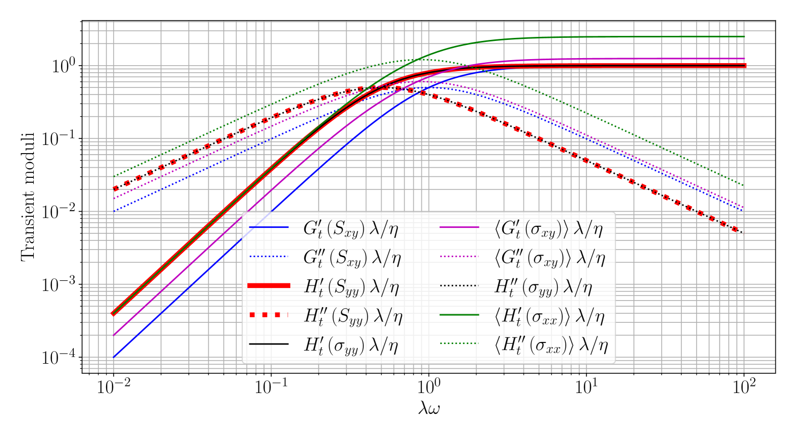
Figure 1: Evolution of the transient moduli of $S_{xy}$, $S_{yy}$ and $\sigma_{yy}$ and the average according to time of transient moduli of $\sigma_{xx}$ and $\sigma_{xy}$, all divided by $\eta/\lambda$ as a function $\lambda\omega$ with $\varepsilon_{0}=1$.

Now if we look at the expressions for $\sigma_{xx}$ and $\sigma_{xy}$, we see that there are non zero contribution of each component. Normally, one would expect only the $\sigma_{xy}$ component to play a role but here, due to the increase of the strain amplitude $\varepsilon_{0}$, additional contributions appear. It is possible to recover the usual linear Maxwell model expressed in terms of the Cauchy stress tensor $\bm{\sigma}$ when $\varepsilon_{0}\to 0$. However, at moderately high strain amplitude, there are variations in time of the various transient moduli. There is the actual novelty of this approach : with the steady-state approach, one would only find the average values over time. Now, one can find some more intricate evolutions to properly understand the materials behaviour. To give some illustrations to those equations, fig.˜2 shows the time evolution of the various transient moduli of $\sigma_{xx}$ and $\sigma_{xy}$ with the parameters $\varepsilon_{0}=\lambda\omega=1$. To give another perspective, fig.˜3 gives the Cole-Cole plot, i.e. the viscous transient moduli as a function of the elastic transient moduli, with the same set of parameters. An interesting thing when looking at fig.˜3 is that, focusing on the black line for $G_{t}\left(\sigma_{xy}\right)$, which is usually observed in experiments presenting the 3 peaks, there exist some portion of the cycle where either or both $G_{t}^{\prime}\left(\sigma_{xy}\right)$ and $G_{t}^{\prime\prime}\left(\sigma_{xy}\right)$ are negative. This is interpreted sometimes as sign of elastic recoil or negative dissipation. However, this example demonstrates that even for a model where the rheological parameters are properly defined without any doubts on thermodynamics, there is some strange behaviour happening which may lead to skewed interpretations. In this case, a simple geometrical transformation of the Cauchy stress tensor $\bm{\sigma}$ into the second Piola-Kirchhoff stress tensor $\bm{S}$ leads to a rheological analysis which is much simpler due to the fact that the newly obtained moduli will be constant and corresponding exactly to a linear Maxwell fluid. All these remarks are just a warning for people who are looking for a characterisation and parameter identification of their materials: some processing may be needed on experimental data to analyse properly the rheological behaviour having taken into account geometrical non linearities.

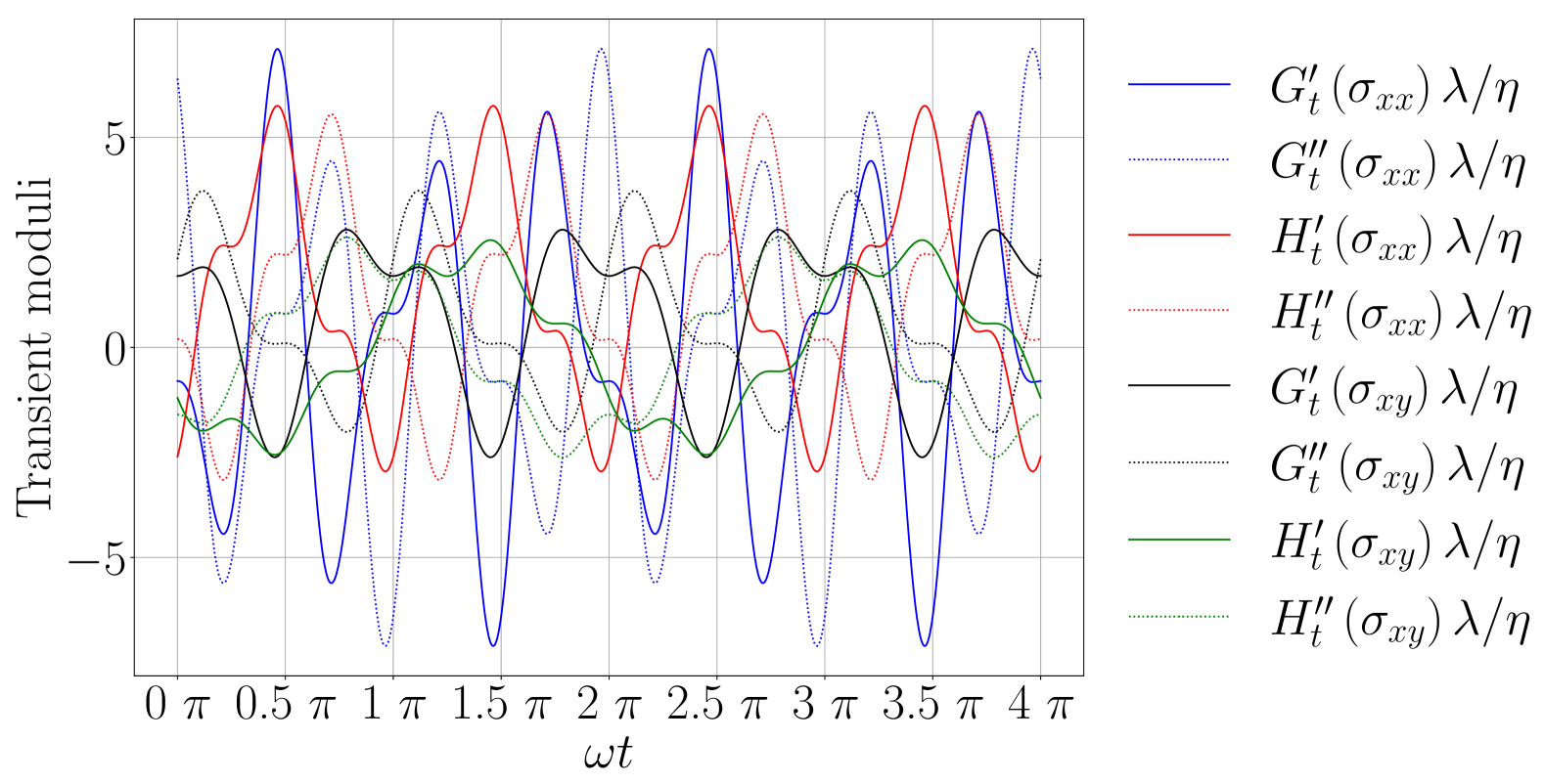
Figure 2: Evolution of the various moduli of $\sigma_{xy}$ and $\sigma_{xx}$ divided by $\eta/\lambda$ as a function $\omega t$ imposing $\lambda\omega=\varepsilon_{0}=1$.

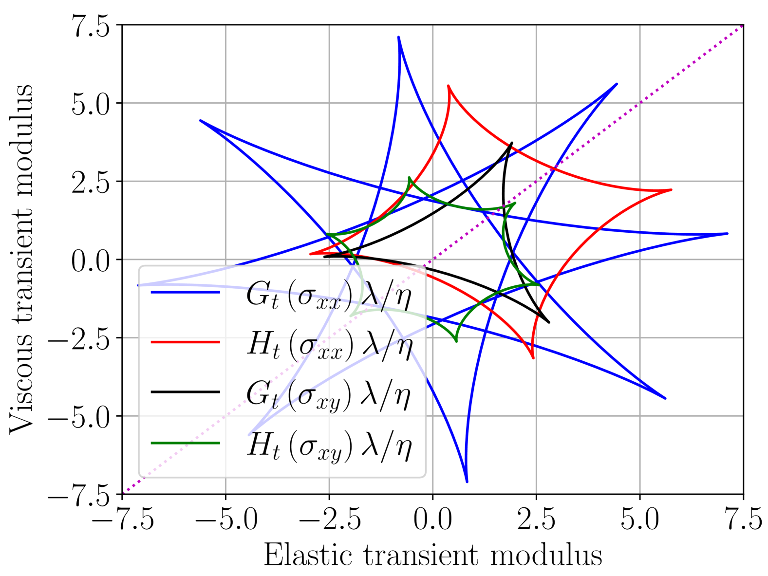
Figure 3: Evolution of the viscous moduli of $\sigma_{xy}$ and $\sigma_{xx}$ divided by $\eta/\lambda$ as a function of the elastic moduli divided by $\eta/\lambda$ imposing $\lambda\omega=\varepsilon_{0}=1$. The purple dotted line corresponds to the first bisector $y=x$.

III.2 Kelvin-Voigt model

Let us consider a Kelvin-Voigt model

$$\bm{S}=2E\bm{e}+2\eta\dot{\bm{e}}.$$ (91)

The equations are then

$$S_{xx} =0,$$ (92)

$$S_{xy} =E\varepsilon+\eta\dot{\varepsilon},$$ (93)

$$S_{xz} =0,$$ (94)

$$S_{yy} =E\varepsilon^{2}+2\eta\varepsilon\dot{\varepsilon},$$ (95)

$$S_{yz} =0,$$ (96)

$$S_{zz} =0.$$ (97)

If one assumes additionally that for all $t\in\mathbb{R}_{+}$, $\varepsilon\left(t\right)=\varepsilon_{0}\sin\left(\omega t\right)$ with $\omega$ a certain pulsation, one gets

$$S_{yy}\left(t\right) =E\varepsilon_{0}^{2}\left(1-\cos\left(2\omega t\right)\right)+\eta\omega\varepsilon_{0}^{2}\sin\left(2\omega t\right),$$ (98)

$$S_{xy}\left(t\right) =E\varepsilon_{0}\sin\left(\omega t\right)+\eta\omega\varepsilon_{0}\cos\left(\omega t\right).$$ (99)

It is again blatant that $S_{yy}\propto\varepsilon_{0}^{2}$ and $S_{xy}\propto\varepsilon_{0}$, thus, when $\varepsilon_{0}\to 0$, $S_{yy}$ will become negligible compared to $S_{xy}$, which is the usual case with small oscillatory shear knowing also that, in this limit, $\sigma_{xy}\approx S_{xy}$. Analysing eqs.˜98 and 99, we recover the usual solution for the shear component $S_{xy}$ replacing $\bm{S}$ by $\bm{\sigma}$ in eq.˜91 ; however, there is an axial component $S_{yy}$ which oscillates with a double frequency $2\omega$ compared to the original strain oscillation. Another interesting fact is that $S_{yy}$ has a non-zero zeroth harmonic which is equal to $E\varepsilon_{0}^{2}$.

Now if we come back to the Cauchy stress tensor, one gets with eqs.˜32, 33, 34, 35, 98 and 99 doing some trigonometric calculations,

$$\sigma_{xx}\left(t\right) =E\varepsilon_{0}^{2}\left(1+\frac{3}{4}\varepsilon_{0}^{2}\right)-E\varepsilon_{0}^{2}\cos\left(2\omega t\right)\left(1+\varepsilon_{0}^{2}\right)$$ (100)

$$+\eta\omega\varepsilon_{0}^{2}\left(1+\frac{\varepsilon_{0}^{2}}{2}\right)\sin\left(2\omega t\right)+\frac{E\varepsilon_{0}^{4}}{4}\cos\left(4\omega t\right)$$ (101)

$$-\frac{\eta\omega\varepsilon_{0}^{4}}{4}\sin\left(4\omega t\right),$$ (102)

$$\sigma_{xy}\left(t\right) =E\varepsilon_{0}\left(1+\frac{3}{2}\varepsilon_{0}^{2}\right)\sin\left(\omega t\right)$$ (103)

$$+\eta\omega\varepsilon_{0}\left(1+\frac{\varepsilon_{0}^{2}}{2}\right)\cos\left(\omega t\right)-\frac{E\varepsilon_{0}^{3}}{2}\sin\left(3\omega t\right)$$ (104)

$$-\frac{\eta\omega\varepsilon_{0}^{3}}{2}\cos\left(3\omega t\right),$$ (105)

$$\sigma_{yy}\left(t\right) =E\varepsilon_{0}^{2}\left(1-\cos\left(2\omega t\right)\right)+\eta\omega\varepsilon_{0}^{2}\sin\left(2\omega t\right).$$ (106)

What is really noteworthy from the equations above is that, in the Cauchy stress tensor, there are non zero $\sigma_{xy}$ and $\sigma_{yy}$ components but also a $\sigma_{xx}$ component. Also, the $\sigma_{yy}$ component remains identical to $S_{yy}$, with the double frequency oscillation, but $\sigma_{xy}$ has two harmonics, the first and the third, and $\sigma_{xx}$ has three harmonics, the zeroth, the second and the fourth. The non-zero average of $\sigma_{xx}$ is equal to

$$\lim_{T\to+\infty}\frac{1}{T}\int_{0}^{T}\sigma_{xx}\left(t\right)\,\mathrm{d}t=E\varepsilon_{0}^{2}\left(1+\frac{3}{4}\varepsilon_{0}^{2}\right).$$ (107)

It is now possible to compare the usual Sequence of Physical Process with the extended version presented here. In the usual Sequence of Physical Process, the transient moduli are calculated through eqs.˜51 and 52 which gives, using the expressions above in the limit $\varepsilon_{0}\to 0$,

$$\mathcal{G}_{t}^{\prime}\left(\sigma_{xy}\right) =E$$ (108)

$$\mathcal{G}_{t}^{\prime\prime}\left(\sigma_{xy}\right) =\eta\omega$$ (109)

as a usual linear Kelvin-Voigt model with the variables $\bm{\sigma}$ and $\bm{\varepsilon}$. Using the new extended version with the second Piola-Kirchhoff tensor, it is possible to obtain for $S_{xy}$,

$$G_{t}^{\prime}\left(S_{xy}\right) =E,$$ (110)

$$G_{t}^{\prime\prime}\left(S_{xy}\right) =\eta\omega,$$ (111)

$$H_{t}^{\prime}\left(S_{xy}\right) =0,$$ (112)

$$H_{t}^{\prime\prime}\left(S_{xy}\right) =0,$$ (113)

and for $S_{yy}$,

$$G_{t}^{\prime}\left(S_{yy}\right) =0,$$ (114)

$$G_{t}^{\prime\prime}\left(S_{yy}\right) =0,$$ (115)

$$H_{t}^{\prime}\left(S_{yy}\right) =E,$$ (116)

$$H_{t}^{\prime\prime}\left(S_{yy}\right) =\eta\omega.$$ (117)

Hence, we find transient moduli both in the shear direction $xy$ and in the axial direction $yy$ with very interesting relationships like

$$H_{t}^{\prime}\left(S_{yy}\right)=G_{t}^{\prime}\left(S_{xy}\right),$$ (118)

$$H_{t}^{\prime\prime}\left(S_{yy}\right)=G_{t}^{\prime\prime}\left(S_{xy}\right).$$ (119)

Another interesting feature which may be highlighted is the fact that, due to construction with eq.˜6 and looking at eqs.˜98, 99, 110, 111, 116 and 117, each component of $\bm{S}$ is a linear combination of $\varepsilon$, $\dot{\varepsilon}/\omega$, $\varepsilon^{2}$ and $2\dot{\varepsilon}\varepsilon/\omega$ with the transient moduli $G_{t}^{\prime}$, $G_{t}^{\prime\prime}$, $H_{t}^{\prime}$ and $H_{t}^{\prime\prime}$ as factors.

It is now possible to find the last moduli for $\sigma_{xx}$, $\sigma_{xy}$ and $\sigma_{yy}$. The easiest one is $\sigma_{yy}$ thanks to eq.˜34 thus

$$G_{t}^{\prime}\left(\sigma_{yy}\right) =0,$$ (120)

$$G_{t}^{\prime\prime}\left(\sigma_{yy}\right) =0,$$ (121)

$$H_{t}^{\prime}\left(\sigma_{yy}\right) =E,$$ (122)

$$H_{t}^{\prime\prime}\left(\sigma_{yy}\right) =\eta\omega.$$ (123)

For $\sigma_{xx}$ and $\sigma_{xy}$, the fourth and the third harmonics, respectively, prevent a quick calculations so the overall framework should be applied. In the case of $\sigma_{xx}$, defining $\tan\left(\alpha\right)=\eta\omega/E$, one gets

$$\frac{G_{t}^{\prime}\left(\sigma_{xx}\right)}{2\varepsilon_{0}^{3}\sqrt{E^{2}+\eta^{2}\omega^{2}}} =3\sin\left(5\omega t+\alpha\right)-5\sin\left(3\omega t+\alpha\right)$$ (124)

$$\frac{G_{t}^{\prime\prime}\left(\sigma_{xx}\right)}{2\varepsilon_{0}^{3}\sqrt{E^{2}+\eta^{2}\omega^{2}}} =3\cos\left(5\omega t+\alpha\right)+5\cos\left(3\omega t+\alpha\right)$$ (125)

$$\frac{H_{t}^{\prime}\left(\sigma_{xx}\right)}{2\sqrt{E^{2}+\eta^{2}\omega^{2}}} =\cos\left(\alpha\right)\left(1+\varepsilon_{0}^{2}\right)+$$ (126)

$$-\frac{5\varepsilon_{0}^{2}}{4}\left(3\cos\left(2\omega t+\alpha\right)+\cos\left(6\omega t+\alpha\right)\right)$$ (127)

$$\frac{H_{t}^{\prime\prime}\left(\sigma_{xx}\right)}{2\sqrt{E^{2}+\eta^{2}\omega^{2}}} =\sin\left(\alpha\right)\left(1+\frac{\varepsilon_{0}^{2}}{2}\right)+$$ (128)

$$+\frac{5\varepsilon_{0}^{2}}{4}\left(\sin\left(6\omega t+\alpha\right)-3\sin\left(2\omega t+\alpha\right)\right)$$ (129)

and for $\sigma_{xy}$, one obtains

$$\frac{G_{t}^{\prime}\left(\sigma_{xy}\right)}{\sqrt{E^{2}+\eta^{2}\omega^{2}}} =\cos\left(\alpha\right)\left(1+\frac{3}{2}\varepsilon_{0}^{2}\right)+$$ (130)

$$-\frac{5\varepsilon_{0}^{2}}{2}\left(\cos\left(4\omega t+\alpha\right)-2\cos\left(2\omega t+\alpha\right)\right)$$ (131)

$$\frac{G_{t}^{\prime\prime}\left(\sigma_{xy}\right)}{\sqrt{E^{2}+\eta^{2}\omega^{2}}} =\sin\left(\alpha\right)\left(1+\frac{\varepsilon_{0}^{2}}{2}\right)+$$ (132)

$$+\frac{5\varepsilon_{0}^{2}}{2}\left(\sin\left(4\omega t+\alpha\right)+2\sin\left(2\omega t+\alpha\right)\right)$$ (133)

$$\frac{H_{t}^{\prime}\left(\sigma_{xy}\right)}{\varepsilon_{0}\sqrt{E^{2}+\eta^{2}\omega^{2}}} =-5\sin\left(\omega t+\alpha\right)-\sin\left(5\omega t+\alpha\right)$$ (134)

$$\frac{H_{t}^{\prime\prime}\left(\sigma_{xy}\right)}{\varepsilon_{0}\sqrt{E^{2}+\eta^{2}\omega^{2}}} =\cos\left(5\omega t+\alpha\right)-5\cos\left(\omega t+\alpha\right)$$ (135)

With the previous equations, it can be interesting to compare the usual Sequence of Physical Processes with the present extended version. Thus, using eqs.˜108 and 109 and the average time values of eqs. 130 to 133, one obtains

$$\left\langle G_{t}^{\prime}\left(\sigma_{xy}\right)\right\rangle-\mathcal{G}_{t}^{\prime}\left(\sigma_{xy}\right) =\frac{3}{2}E\varepsilon_{0}^{2}$$ (136)

$$\left\langle G_{t}^{\prime\prime}\left(\sigma_{xy}\right)\right\rangle-\mathcal{G}_{t}^{\prime\prime}\left(\sigma_{xy}\right) =\frac{\eta\omega\varepsilon_{0}^{2}}{2}.$$ (137)

To give more clarity of understanding, it is possible to plot the variations of these moduli according to different parameters. Noting that the moduli of $S_{xy}$, $S_{yy}$ and $\sigma_{yy}$ are constant with time, the table˜1 illustrates the summary of the expressions of those moduli. We recognise the usual Kelvin-Voigt model expressions with some additional items due to the geometrical complements of the Piola-Kirchhoff expressions.

Transient moduli	$\bullet_{t}^{\prime}$	$\bullet_{t}^{\prime\prime}$
$G_{t}\left(S_{xy}\right)$	$E$	$\eta\omega$
$H_{t}\left(S_{yy}\right)$	$E$	$\eta\omega$
$H_{t}\left(\sigma_{yy}\right)$	$E$	$\eta\omega$
$\left\langle H_{t}\left(\sigma_{xx}\right)\right\rangle$	$2E\left(1+\varepsilon_{0}^{2}\right)$	$2\eta\omega\left(1+\dfrac{\varepsilon_{0}^{2}}{2}\right)$
$\left\langle G_{t}\left(\sigma_{xy}\right)\right\rangle$	$E\left(1+\dfrac{3}{2}\varepsilon_{0}^{2}\right)$	$\eta\omega\left(1+\dfrac{\varepsilon_{0}^{2}}{2}\right)$

Table 1: Summary of the expressions of the transient moduli for $S_{xy}$, $S_{yy}$ and $\sigma_{yy}$ and the average overtime of the transient moduli for $\sigma_{xx}$ and $\sigma_{xy}$ according to eqs.˜110, 111, 117, 116, 123, 122, 126, 128, 130 and 132.

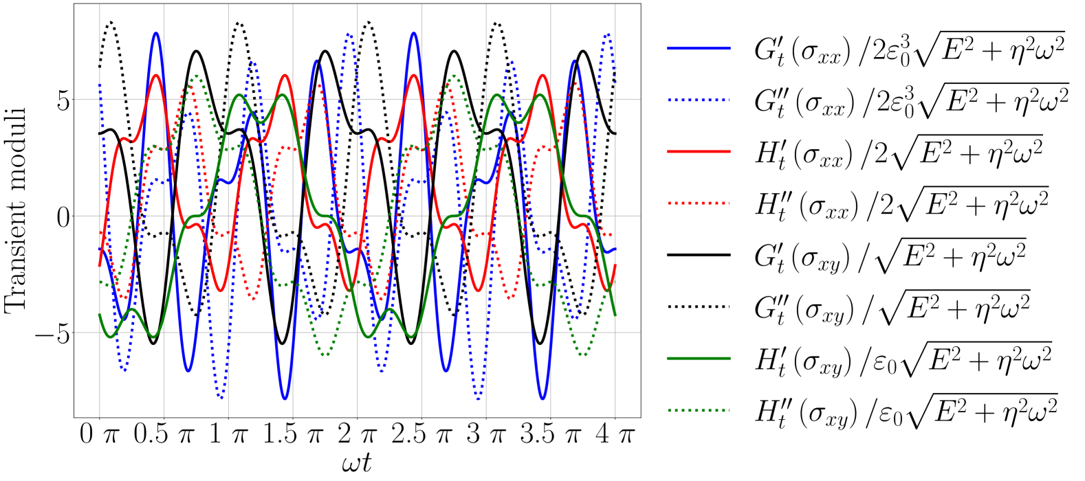
Figure 4: Evolution of the various moduli $G^{\prime}_{t}$, $G^{\prime\prime}_{t}$, $H^{\prime}_{t}$ and $H^{\prime\prime}_{t}$ of $\sigma_{xy}$ and $\sigma_{xx}$ divided, respectively, by $2\varepsilon_{0}^{3}\sqrt{E^{2}+\eta^{2}\omega^{2}}$, $2\sqrt{E^{2}+\eta^{2}\omega^{2}}$, $\sqrt{E^{2}+\eta^{2}\omega^{2}}$ and $\varepsilon_{0}\sqrt{E^{2}+\eta^{2}\omega^{2}}$ as a function $\omega t$ imposing $E/\eta\omega=\varepsilon_{0}=1$.

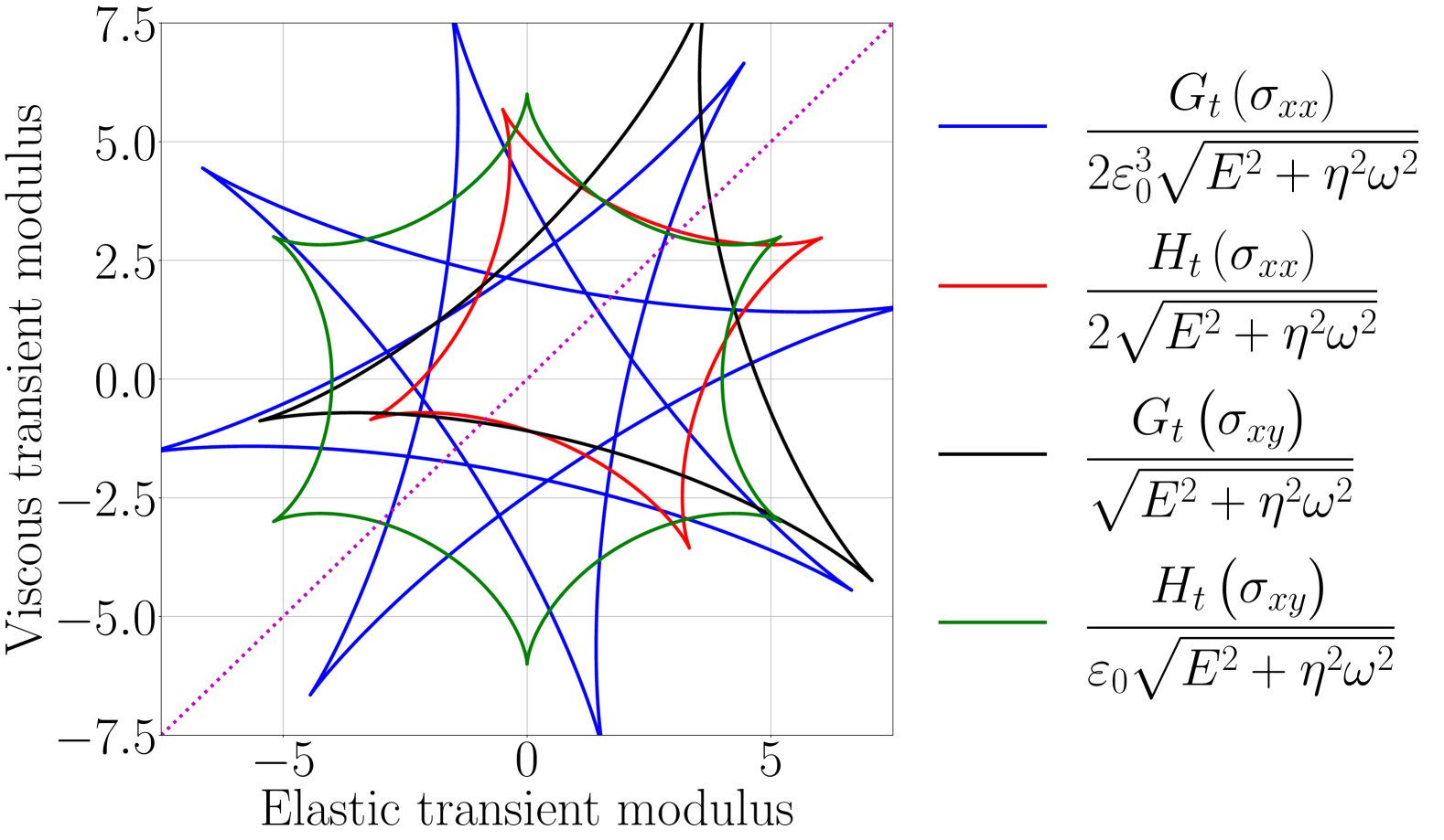
Figure 5: Evolution of the viscous moduli $G^{\prime\prime}_{t}$ and $H^{\prime\prime}_{t}$ of $\sigma_{xy}$ and $\sigma_{xx}$ divided, respectively, by $2\varepsilon_{0}^{3}\sqrt{E^{2}+\eta^{2}\omega^{2}}$, $2\sqrt{E^{2}+\eta^{2}\omega^{2}}$, $\sqrt{E^{2}+\eta^{2}\omega^{2}}$ and $\varepsilon_{0}\sqrt{E^{2}+\eta^{2}\omega^{2}}$ as a function of the elastic moduli $G^{\prime}_{t}$ and $H^{\prime}_{t}$ of $\sigma_{xy}$ and $\sigma_{xx}$ divided, respectively, by $2\varepsilon_{0}^{3}\sqrt{E^{2}+\eta^{2}\omega^{2}}$, $2\sqrt{E^{2}+\eta^{2}\omega^{2}}$, $\sqrt{E^{2}+\eta^{2}\omega^{2}}$ and $\varepsilon_{0}\sqrt{E^{2}+\eta^{2}\omega^{2}}$ imposing $E/\eta\omega=\varepsilon_{0}=1$. The purple dotted line corresponds to the first bisector $y=x$.

Now if we look at the expressions for $\sigma_{xx}$ and $\sigma_{xy}$, we see that there are non zero contribution of each component. Normally, one would expect only the $\sigma_{xy}$ component to play a role but here, due to the increase of the strain amplitude $\varepsilon_{0}$, additional contributions appear. It is possible to recover the usual linear Kelvin-Voigt model expressed in terms of the Cauchy stress tensor $\bm{\sigma}$ when $\varepsilon_{0}\to 0$. However, at high strain amplitude, there are variations in time of the various transient moduli. So here is the actual novelty of this approach because, with the steady-state approach, one would only find the average values over time. Now, one can find some more intricate evolutions to properly understand the behaviour of the materials. To give some illustrations to those equations, fig.˜4 shows the time evolution of the various transient moduli of $\sigma_{xx}$ and $\sigma_{xy}$ with the parameters $\varepsilon_{0}=E/\eta\omega=1$. To give another perspective, the fig.˜5 gives the Cole-Cole plot, i.e. the viscous transient moduli as a function of the elastic transient moduli, with the same set of parameters. An interesting thing when looking at fig.˜5 is that, focusing on the black line for $G_{t}\left(\sigma_{xy}\right)$, which is usually observed in experiments presenting 3 peaks, there exist some portion of the cycle where either or both $G_{t}^{\prime}\left(\sigma_{xy}\right)$ and $G_{t}^{\prime\prime}\left(\sigma_{xy}\right)$ are negative. This is interpreted sometimes as sign of elastic recoil or negative dissipation. However, this example demonstrates that even for a model where the rheological parameters are properly defined without any doubts on thermodynamics, there is some strange behaviour happening which may lead skewed interpretations. In this case, a simple geometrical transformation of the Cauchy stress tensor $\bm{\sigma}$ into the second Piola-Kirchhoff stress tensor $\bm{S}$ leads to a rheological analysis which is much simpler due to the fact that the newly obtained moduli will be constant and corresponding exactly to a linear Kelvin-Voigt fluid. All these remarks are just a warning for people who are looking for a characterisation and an identification of their materials: some processing may be needed on experimental data to analyse properly the rheological behaviour having taken into account geometrical non linearities.

We can carry out the overall analysis as in [19, 20, 21, 22, 23] but we leave the rest of the comparison to the reader.

In general, what is interesting is that when $\varepsilon_{0}\gg 1$, the main stress components are $\sigma_{xx}$ first due to the proportionality to $\varepsilon_{0}^{4}$, then $S_{yy}$, $\sigma_{xy}$ and $\sigma_{yy}$ with the proportionality to $\varepsilon_{0}^{2}$ and finally, the shear components $S_{xy}$ which is linear in $\varepsilon_{0}$.

IV How to use this framework experimentally

All the previous demonstrations may seem really theoretical when compared to actual complex behaviour observed in experiments. Therefore, any experimental researcher may wonder how the understanding of rheology is enhanced by such framework. To answer this item, it is interesting to note that experiments are carried in real time: that is to say, all the quantities are measured in the current configuration, omitting the conditions of the initial configuration. Hence, to rationalise the observed behaviour, it is relevant to come back to the initial configuration to follow what has happened since the beginning of the experiment both macroscopically and microspically. From this objective, concretely, for example, the stresses may be measured through any device to compute $\bm{\sigma}$ and come back to the original stresses in the initial configuration $\bm{S}$ using the transformation given by eq.˜4 in the case of a plan shear in the $xy$ plane. Hence, displaying the values of $\bm{S}$ instead of $\bm{\sigma}$ will bring a different perspective to the interpretation of stresses. Then, trying to find a relationship between $\bm{S}$ and $\bm{e}$ and its derivatives instead of $\bm{\varepsilon}$ and its derivatives can expand the field of possibilities and a broader understanding of the evolution of materials. It may not be as simple and confortable than a 1D variable like $\bm{\sigma}$ and $\bm{\varepsilon}$ but materials are dived in 3D space and inherit most of their properties from this initial description. Consequently, omitting this 3D dependence may lead to misunderstanding of the actual physics of rheology which was highlighted in this paper.

Furthermore, all the previous discussion can only happen when the experimental data are of high quality. Corrections of non linearities are indeed useful when there is a complete control of the materials behaviour in terms of data accuracy and data exhaustiveness

V Conclusion

To put it in a nutshell, this paper has extended the usual Sequence of Physical Processes framework developed by [19] taking into account geometrical non linearities and geometrical corrections through the use of the second Piola-Kirchhoff stress tensor and the Green-Lagrange strain tensor. Applying the global framework to two very classical linear viscoelastic models showed how a simple rheological relation may bring much more complex observations in the current configuration. The last section highlighted this point inviting researchers investigating large amplitude oscillations to study the rheology of certain materials to properly account for geometrical non linearities before trying to conclude on certain observations.

The main point of this paper is to point out that the initial choices of a representation, which can be the pure rheological model but also the intuition of the actual flow in a rheometer for example, are decisive. In this sense, starting with what can be seen a posteriori as the wrong representation may force to carry on heavy artifacts which can be counterproductive. It must be remembered that the simplest descriptions, in terms of calculations and number of parameters, are usually the best to be able to interpret as simply as possible the very intricate phenomena we observe.

A more general comment is that when we study large deformations in rheology or mechanics, heterogeneities in the deformations or in the flow profile may appear and lead to wrong interpretations. A closer look must happen to carefully pay attention to both the rheological measurements and the actual physics of the movement.

References

- Landau and Lifshitz [1959] L. D. Landau and E. M. Lifshitz, Theory of Elasticity, 1st ed., edited by L. D. Landau and E. M. Lifshitz, Vol. 7 (Pergamon Press, Pergamon Press LTD., 4 and 5 Fitzroy Square, London W.1, 1959).
- Landau and Lifshitz [1987] L. D. Landau and E. M. Lifshitz, Fluid Mechanics, deuxième ed., edited by L. D. Landau and E. M. Lifshitz, Course of Theoretical Physics, Vol. 6 (Pergamon Press, Institute of Physical Problems, U.S.S.R. Academy of Sciences, 1987).
- Barber [2004] J. R. Barber, Elasticity, 3rd ed., edited by J. R. Barber, Solid Mechanics and its applications, Vol. 107 (Springer Dordrecht, 2004).
- Bird, Stewart, and Lightfoot [2002] R. B. Bird, W. E. Stewart, and E. N. Lightfoot, Transport Phenomena, deuxième ed., edited by R. B. Bird, W. E. Stewart, and E. N. Lightfoot (John Wiley and Sons, Chemical Engineering Department University of Wisconsin-Madison, 2002).
- von Mises [1913] R. von Mises, “Mechanik der festen Körper im plastisch-deformablen Zustand,” Nachrichten von der Gesellschaft der Wissenschaften zu Göttingen 1, 582–592 (1913).
- Tresca [1864] H. Tresca, “Mémoires sur l’écoulement des corps solides soumis à de fortes pressions,” Compte Rendus à l’Académie des Sciences de Paris 59, 754 (1864).
- Bingham [1922] E. C. Bingham, Fluidity and Plasticity, 1st ed., edited by E. C. Bingham (McGraw-Hill Book company, Anna, 1922).
- Ostwald [1925] W. Ostwald, “Ueber die Geschwindigkeitsfunktion der Viskosität disperser Systeme. I,” Kolloid-Zeitschrift 36, 99–117 (1925).
- Herschel and Bulkley [1926] V. W. H. Herschel and R. Bulkley, “Ronsistenzmessungen yon Gummi-Benzollösungen,” Kolloid-Zeitschrift 39, 291–300 (1926).
- Maxwell [1867] J. C. Maxwell, “IV. On the dynamical theory of gases,” Philosophical Transactions of the Royal Society of London 157, 49–88 (1867), https://royalsocietypublishing.org/doi/pdf/10.1098/rstl.1867.0004 .
- Kelvin, Larmor, and Joule [1890] W. T. B. Kelvin, J. Larmor, and J. P. Joule, Mathematical and Physical Papers: Elasticity, heat, electro-magnetism, Mathematical and Physical Papers (University Press, 1890).
- Voigt [1890] W. Voigt, “Ueber die innere Reibung der festen Körper, insbesondere der Krystalle,” Abhandlungen der Königlichen Gesellschaft der Wissenschaften in Göttingen 36, 3–48 (1890).
- Halphen and Nguyen [1975] B. Halphen and Q. S. Nguyen, “Sur les matériaux standards généralisés,” Journal de Mécanique 14, 39–63 (1975).
- Wang and Selomulya [2022] Y. Wang and C. Selomulya, “Food rheology applications of large amplitude oscillation shear (LAOS),” Trends in Food Science & Technology 127, 221–244 (2022).
- Grotian genannt Klages et al. [2022] H. Grotian genannt Klages, N. Ermis, G. A. Luinstra, and K. M. Zentel, “Coupling Kinetic Modelling with SAOS and LAOS Rheology of Poly(n-butyl acrylate),” Macromolecular Rapid Communications 43, 2100620 (2022), https://onlinelibrary.wiley.com/doi/pdf/10.1002/marc.202100620 .
- Lopez and Richtering [2021] C. G. Lopez and W. Richtering, “Oscillatory rheology of carboxymethyl cellulose gels: Influence of concentration and pH,” Carbohydrate Polymers 267, 118117 (2021).
- Bergman et al. [2011] T. L. Bergman, A. S. Lavine, F. P. Incropera, and D. P. Dewitt, Fundamentals of Heat and Mass Transfert, 7th ed., edited by T. L. Bergman, A. S. Lavine, F. P. Incropera, and D. P. Dewitt (John Wiley & Sons, 2011).
- Bhatti and Shah [1987] M. S. Bhatti and R. K. Shah, “Handbook of single-phase convective heat transfer,” (John Wiley & Sons, 1987) Chap. Turbulent and Transition Flow Convective Heat Transfer in Ducts, pp. 1–166.
- Rogers [2017] S. A. Rogers, “In search of physical meaning: defining transient parameters for nonlinear viscoelasticity,” Rheology Acta 56, 501–525 (2017).
- Donley et al. [2019] G. J. Donley, J. R. de Bruyn, G. H. McKinley, and S. A. Rogers, “Time-resolved dynamics of the yielding transition in soft materials,” Journal of Non-Newtonian Fluid Mechanics 264, 117–134 (2019).
- Rogers et al. [2011] S. A. Rogers, B. M. Erwin, D. Vlassopoulos, and M. Cloitre, “A sequence of physical processes determined and quantified in LAOS: Application to a yield stress fluid,” Journal of Rheology 55, 435–458 (2011), https://doi.org/10.1122/1.3544591 .
- Rogers and Lettinga [2012] S. A. Rogers and M. P. Lettinga, “A sequence of physical processes determined and quantified in large-amplitude oscillatory shear (LAOS): Application to theoretical nonlinear models,” Journal of Rheology 56, 1–25 (2012), https://doi.org/10.1122/1.3662962 .
- Rogers [2012] S. A. Rogers, “A sequence of physical processes determined and quantified in LAOS: An instantaneous local 2D/3D approach,” Journal of Rheology 56, 1129–1151 (2012), https://doi.org/10.1122/1.4726083 .
- Note [1] It may be interesting to comment that in the case of incompressible deformations, at every time.
- Le Tallec [2019] P. Le Tallec, Mécanique des milieux continus II, edited by P. Le Tallec (École Polytechnique, 2019).