Hints of Primordial Magnetic Fields at Recombination and Implications for the Hubble Tension

Abstract

Primordial Magnetic Fields (PMFs), long studied as potential relics of the early Universe, accelerate the recombination process and have been proposed as a possible way to relieve the Hubble tension. However, previous studies relied on simplified toy models. In this study, for the first time, we use the recent high-precision evaluations of recombination with PMFs, incorporating full magnetohydrodynamic (MHD) simulations and detailed Lyman-alpha radiative transfer, to test PMF-enhanced recombination ($b\Lambda$CDM) against observational data from the cosmic microwave background (CMB), baryon acoustic oscillations (BAO), and Type Ia supernovae (SN). Focusing on non-helical PMFs with a Batchelor spectrum, we find a preference for present-day total field strengths of approximately 5-10 pico-Gauss. Depending on the dataset combination, this preference ranges from mild ($\sim 1.8\sigma$ with Planck + DESI) to moderate ($\sim 3\sigma$ with Planck + DESI + SH0ES-calibrated SN) significance. The $b\Lambda$CDM has Planck + DESI $\chi^{2}$ values equal or better than those of the $\Lambda$CDM model while predicting a higher Hubble constant. The favored field strengths align closely with those required for cluster magnetic fields to originate entirely from primordial sources, without the need for additional dynamo amplification or stellar magnetic field contamination. Future high-resolution CMB temperature and polarization measurements will be crucial for confirming or further constraining the presence of PMFs at recombination.

I Introduction

With cosmology entering the era where multiple independent datasets are able to constrain key aspects of the cosmological model with precision comparable to that of the cosmic microwave background (CMB), tensions between certain datasets have emerged in the context of the $\Lambda$ Cold Dark Matter ($\Lambda$CDM) model. Most prominent among them is “the Hubble tension” – a $5\sigma$ discrepancy between the value of the Hubble constant, $H_{0}=67.36\pm 0.54$ km/s/Mpc, inferred from the Planck CMB data Aghanim et al. (2020), and $H_{0}=73.04\pm 1.04$ km/s/Mpc measured by the SH0ES collaboration using supernovae Type Ia (SN) calibrated on Cepheid stars observed by the Hubble Space Telescope (HST) Riess et al. (2022a, b). SN calibrations using Tip of the Red Giant Branch (TRGB) stars, J-Region Asymptotic Giant Branch (JAGB) stars, and Cepheids from the James Webb Space Telescope (JWST) also yield larger $H_{0}$ Freedman et al. (2024), albeit with larger uncertainties, with the uncertainties expected to shrink considerably as more JWST data becomes available. A lesser tension concerns measurements of the matter clustering amplitude quantified by the parameter $S_{8}$. The Planck-CMB-inferred value is $S_{8}=0.832\pm 0.013$, while the joint analysis of galaxy counts and galaxy weak lensing data Abbott et al. (2023) from the Dark Energy Survey Year 3 (DES-Y3) Amon et al. (2022) and Kilo-Degree Survey (KiDS-1000) Asgari et al. (2021) yields $S_{8}=0.790^{+0.018}_{-0.014}$. Another minor tension emerged recently between the value of the matter density fraction, $\Omega_{m}$, obtained from uncalibrated SN luminosities and that from the Baryon Acoustic Oscillations (BAO) measurements. The Pantheon+ (PP) SN data yields $\Omega_{m}=0.334\pm 0.018$ Brout et al. (2022), in good agreement with DES-Y5 Abbott et al. (2024) and Union3 Rubin et al. (2023) SN datasets, while the BAO measurements by the Dark Energy Spectroscopic Instrument (DESI) give $\Omega_{m}=0.295\pm 0.015$ Adame et al. (2024).

The Hubble tension generated significant interest in extensions of the $\Lambda$CDM model Abdalla et al. (2022). Of special interest was the realization that Primordial Magnetic Fields (PMFs), if present in the pre-recombination plasma, would generate baryon inhomogeneities and speed up the recombination process  Jedamzik and Abel (2013), bringing the CMB-deduced value of $H_{0}$ closer to that found from distance-ladders Jedamzik and Pogosian (2020). These findings, reproduced by other groups Thiele et al. (2021); Rashkovetskyi et al. (2021), were based on a simple toy-model of baryon clumping. Unlike many specially designed solutions to the Hubble tension, PMFs have been a subject of continuous study over many decades as the possible source of observed galactic and cluster magnetic fields Widrow (2002). Interest in PMFs increased with tentative evidence for magnetic fields in the extragalactic space from non-observation of GeV $\gamma$-ray halos around TeV blazars Neronov and Vovk (2010) and the synchrotron emission from a few-Mpc-long ridge connecting two merging clusters of galaxies Govoni et al. (2019). However, with non-primordial astrophysical explanations of these low-redshift observations being difficult to rule out Broderick et al. (2018), the only sure way to prove the primordial origin of cosmic magnetic fields would be to find their signatures in the CMB. For a long time, CMB-based studies of PMFs have only led to $\sim$ nano-gauss (nG) upper bounds on the comoving field strength Ade et al. (2016); Zucca et al. (2017), until the realization that the effects of baryon clumping on recombination may strengthen such upper limits by up to two orders of magnitude Jedamzik and Saveliev (2019).

Another significant development happened in the past four years that, together with baryon clumping, has taken PMF studies to a new level. Finding viable models of primordial magnetogenesis proved challenging, with inflationary magnetogenesis requiring postulating new physics to break the conformal invariance of electromagnetism Turner and Widrow (1988); Ratra (1992); Durrer and Neronov (2013), while PMFs generated in phase transitions Vachaspati (1991, 2021), until recently, were not expected to leave observable signatures in the CMB Wagstaff and Banerjee (2016). The prediction for phase-transition-generated PMFs depends crucially on the evolution of the field between the epoch of magnetogenesis and recombination. Leaning on analogies with hydrodynamics, Ref. Banerjee and Jedamzik (2004) formulated such an evolutionary model. However, recent detailed studies Hosking and Schekochihin (2021) of freely decaying MHD turbulence show that the analogy with hydrodynamics is not perfect. The authors of Hosking and Schekochihin (2021) proposed (see also Brandenburg et al. (2015); Zrake (2014)) that even non-helical magnetic fields undergo an inverse cascade governed by the conservation of a new invariant named “Hosking integral”, and that the time-scale of evolution is not governed by the Alfven time-scale but the much slower magnetic reconnection time-scale. The first claim was then subsequently confirmed by Zhou et al. (2022), whereas the second claim has not been found to be correct, although a significantly slower evolution time-scale was found than that previously assumed in Brandenburg et al. (2024). It is important to note that such studies cannot currently be performed for realistic Lundquist numbers relevant to the early universe plasma, but they indicate that phase-transition-generated PMFs may well evolve to produce enough PMF strength to relieve the Hubble tension and explain extragalactic magnetic fields Hosking and Schekochihin (2023).

Earlier studies of the PMF effects on recombination and their impact on CMB anisotropies were based on simple toy models, which moreover did not have a straightforward relation to the final magnetic field strength. With future CMB temperature and polarization experiments promising to distinguish deviations from standard recombination at a few-percent level Lee et al. (2023); Lynch et al. (2024a, b); Mirpoorian et al. (2024), a need for more detailed theoretical modelling of the recombination process in the presence of PMFs emerged. Significant progress in this direction was made over the past two years. Extensive 3D MHD simulations combined with Lyman-$\alpha$ photon transport were performed in Jedamzik et al. (2023) to determine the redshift evolution of the ionized fraction $x_{e}(z)$ from $z=4500$ to $z=10$ for non-helical PMFs with a Batchelor spectrum. In this paper, for the first time, we use the MHD-derived $x_{e}(z)$ in the appropriately modified standard Boltzmann code CAMB Lewis et al. (2000) to compute CMB anisotropy spectra and derive constraints on the PMF and the Hubble constant from the available data.

II Results

We present our constraints on PMFs in terms of the total (i.e. integrated over all scales) root-mean-square comoving field strength $b_{\rm pmf}$ at $z=10$ corresponding to the final time of the MHD simulations Jedamzik et al. (2023). The corresponding field strength at recombination, evaluated at the peak of the visibility function ($z\approx 1090$), is approximately a factor of ten larger. This is due to additional damping that takes place shortly after recombination as the plasma transforms from highly viscous to turbulent state. Weaker, logarithmic damping occurs between $z\approx 100$ and $z=0$ Banerjee and Jedamzik (2004), which means the present-day PMF is comparable to $b_{\rm pmf}$, but about 17% smaller. We refer to $\Lambda$CDM with a PMF as the $b\Lambda$CDM model.

Details of the computations of the ionization history are given in Sec. IV.1 and Sec. IV.2 of Methods. In deriving the constraints on PMFs, we used the mean ionization histories obtained by averaging over 5 MHD realizations at each magnetic strength. This method does not account for the considerable sample variance around the mean predictions. To estimate just how much of a difference this makes, we separately performed a parameter fit using simulations with randomly generated ionization histories based on the MHD-derived covariance. The details of this investigation are presented in Sec. IV.3 of Methods, where we show that, as expected, accounting for the sample variance increases the uncertainty in $b_{\rm pmf}$, while the uncertainties in $H_{0}$ and other cosmological parameters remain largely unchanged.

	$\chi^{2}_{b\Lambda{\rm CDM}}-\chi^{2}_{\Lambda{\rm CDM}}$	$b_{\rm pmf}$ [nG]
PL	$-1.7$	$0.0029\pm 0.0021$
PL+DESI	$-4.7$	$0.0042\pm 0.0023$
PL+DESI+PP	$-3.83$	$0.0038\pm 0.0021$
PL+DESI+ACT	$-5.3$	$0.0030\pm 0.0017$
PL+DESI+SPT	$-5.2$	$0.0036\pm 0.0019$
PL+DESI+PP+$M_{b}$	$-15.25$	$0.0096\pm 0.0032$
PL+DESI+ACT+PP+$M_{b}$	$-11.8$	$0.0064\pm 0.0021$
PL+DESI+SPT+PP+$M_{b}$	$-17.8$	$0.0074\pm 0.0024$

Table 1: Differences in $\chi^{2}$ between $b\Lambda$CDM and $\Lambda$CDM fits to Planck (PL), and combinations of PL with DESI BAO, uncalibrated Pantheon+ (PP) SN, and PP calibrated using the SH0ES value of the absolute magnitude, (PP+$M_{b}$), along with the corresponding best fit $z=10$ PMF strengths $b_{\rm pmf}$. The corresponding PMF strengths at the epoch of recombination are about an order of magnitude larger (See Table 3 in Methods).

	$\Lambda$CDM PL+DESI	$b\Lambda$CDM PL+DESI	$b\Lambda$CDM PL+DESI+PP+$M_{b}$
$b_{\rm pmf}$ [nG]	-	$0.0042\pm 0.0023$	$0.0096\pm 0.0032$
$H_{0}$ [km/s/Mpc]	$67.88\pm 0.37$	$68.52\pm 0.57$	$69.93\pm 0.58$
$\Omega_{m}$	$0.3066\pm 0.0049$	$0.3024\pm 0.0055$	$0.2917\pm 0.0048$
$S_{8}$	$0.8154\pm 0.0090$	$0.8154\pm 0.0090$	$0.8095\pm 0.0087$
$\chi^{2}_{\rm Planck}$	$10973.9$	$10971.6$	$10977.6$
$\chi^{2}_{\rm DESI}$	$16.55$	$14.0728$	$12.91$
$\chi^{2}_{\rm Planck+DESI}$	$10990.4$	$10985.7$	$10990.5$

Table 2: The mean values and standard deviations of $b_{\rm pmf}$, $H_{0}$, $S_{8}$ and $\Omega_{m}$ obtained from PL+DESI and PL+DESI+PP+$M_{b}$, along with the best-fit $\chi^{2}$ values for PL, DESI and PL+DESI.

Table 1 summarizes the mean values and the standard deviations of $b_{\rm pmf}$ obtained from all the different data combinations considered in this work, along with the improvements in the combined $\chi^{2}$ relative to the corresponding $\Lambda$CDM model fits. The datasets are described in Sec. IV.4 of Methods. We find that the Planck (PL) data by itself shows $\sim 1\sigma$ preference for $b_{\rm pmf}$, yielding $0.0029\pm 0.0021$ nG and only a modest improvement of $-1.7$ in the $\chi^{2}$ after adding one new model parameter.

Combining Planck with DESI BAO, shows a minor preference for a non-zero PMF, $b_{\rm pmf}=0.0042\pm 0.023$, while reducing the combined PL+DESI $\chi^{2}$ by $4.7$. This is driven by the well-known preference of the DESI Year 1 data for a larger product of the Hubble constant and the sound horizon at baryon decoupling $r_{\rm drag}h$ Adame et al. (2024) compared to the Planck $\Lambda$CDM derived value (see also Table 5 in Supplemental Material). Accounting for the PMFs allows for larger CMB-derived $r_{\rm drag}h$ values, bringing CMB and BAO in better agreement with each other Pogosian et al. (2024).

Combining Planck and DESI data with uncalibrated SN from Pantheon+ (PP) reduces the evidence for PMFs somewhat due to PP favouring a larger $\Omega_{m}$. However, further combing it with the distance-ladder-determined SN magnitude $M_{b}$ from SH0ES (“the SH0ES prior”), yields $b_{\rm pmf}=0.0096\pm 0.0032$ nG, a $3\sigma$ detection of PMF with $H_{0}=69.93\pm 0.58$ km/s/Mpc, while reducing the combined $\chi^{2}$ by $15.25$.

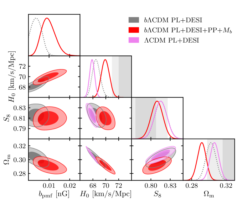
Figure 1: The marginalized $68$% and $95$% CL for mean $x_{e}(z)$ runs for Planck+DESI, Planck+DESI+PP+Mb, and the $\Lambda$CDM fit to Planck+DESI. Shown with grey bands are the 68% and 95& CL bands for the $H_{0}$ measurement by SH0ES Riess et al. (2022a), $S_{8}$ from DES+KiDS Asgari et al. (2021), and $\Omega_{m}$ from PP Brout et al. (2022).

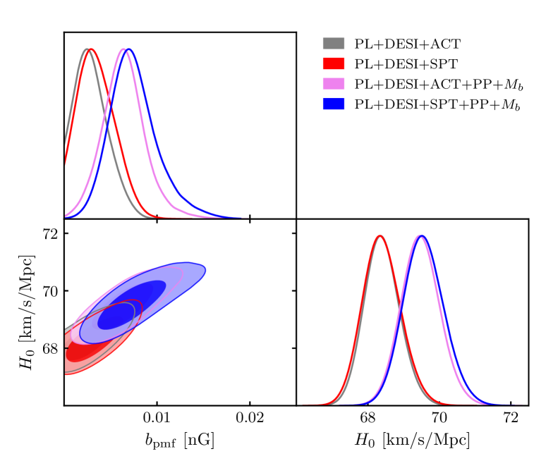
Figure 2: The marginalized $68$% and $95$% CL for $b_{\rm pmf}$ and $H_{0}$ from fits to Planck+DESI+ACT and Planck+DESI+SPT with and without the “SH0ES prior”, PP+$M_{b}$.

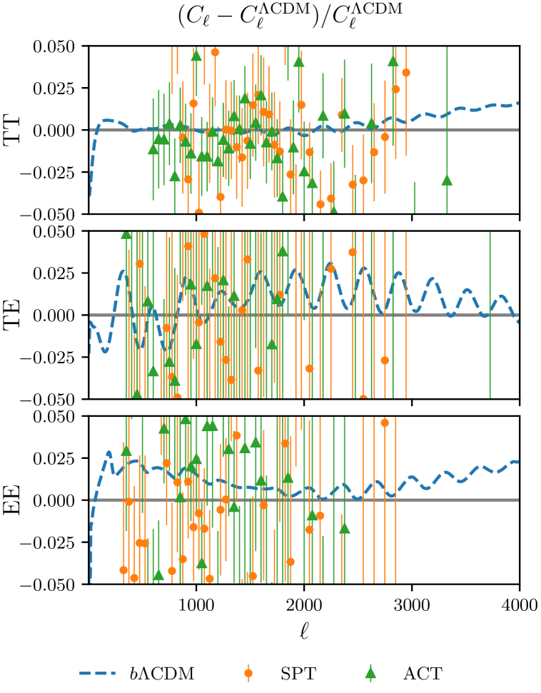
Figure 3: The CMB TT, TE and EE residuals for the best-fit Planck+DESI+PP+$M_{b}$ $b\Lambda$CDM model relative to the $\Lambda$CDM best-fit to Planck+DESI, along with the ACT and SPT band-powers.

The reduction in the PL+DESI+PP+$M_{b}$ $b\Lambda$CDM $\chi^{2}$ is dominated by the improvement in the SH0ES fit, bringing the Hubble tension down to $2.7\sigma$. Interestingly, the fit to the combination of CMB and BAO is as good as for $\Lambda$CDM, with the worsening of the Planck $\chi^{2}$ compensated by the improvement in the DESI fit. This can be seen from Table 2 that lists the mean values and standard deviations in $b_{\rm pmf}$, $H_{0}$, $S_{8}$ and $\Omega_{m}$ obtained from PL+DESI and PL+DESI+PP+$M_{b}$, along with the best fit PL, DESI and PL+DESI $\chi^{2}$ values, comparing them to those from the $\Lambda$CDM PL+DESI fit.

Fig. 1, along with Table 2, shows that the potential detection of the PMF is accompanied by a partial relief for both the $H_{0}$ and the $S_{8}$ tensions. It worsens the $\Omega_{m}$ tension with the SN data, which is the case for any modified recombination solution to the Hubble tension Lee et al. (2023); Poulin et al. (2024); Mirpoorian et al. (2024). There are good reasons to expect the $\Omega_{m}$ problem to be entirely separate from the Hubble tension and any physics at recombination. We note that the $\Omega_{m}$ tension can be interpreted as evidence for dynamical dark energy Adame et al. (2024) which, however, favours an even lower $H_{0}$.

As previously noted in Thiele et al. (2021); Rashkovetskyi et al. (2021); Galli et al. (2022), the CMB temperature and anisotropy spectra on very small angular scales, deep in the Silk damping tail, could be a powerful discriminant of the PMF proposal and other modified recombination models. With this in mind, we perform additional fits to the publicly available high-resolution CMB spectra from ACT Aiola et al. (2020) and SPT Balkenhol et al. (2023). Fig. 2 shows the posteriors for $b_{\rm pmf}$ and $H_{0}$ from fits to Planck+DESI+ACT and Planck+DESI+SPT, with and without the “SH0ES prior”. The corresponding $b_{\rm pmf}$ values and improvements in $\chi^{2}$ are provided in Table 1, while the full parameter tables are provided in Supplemental Material. While both ACT and SPT generally constrain $b_{\rm pmf}$ to smaller values, given the high sensitivity of the small-scale CMB anisotropies to the minute details of the ionization history Mirpoorian et al. (2024), it is remarkable that the MHD-derived $x_{e}(z)$ still provide a good fit.

Fig. 3 shows the CMB spectra residuals, i.e. the relative differences in $C_{\ell}^{TT}$, $C_{\ell}^{TE}$ and $C_{\ell}^{EE}$, for the best-fit PL+DESI+PP+$M_{b}$ $b\Lambda$CDM model relative to the PL+DESI best-fit $\Lambda$CDM model, along with the ACT and SPT data. The differences are at a few-percent level that will be well-within the constraining power of future CMB datasets from the Simons Observatory Aguirre et al. (2018) and CMB-S4 Abazajian et al. (2019).

III Discussion

Using the most comprehensive evaluations of recombination in the presence of PMFs to date, our analysis shows that PMF-accelerated recombination is moderately favored by the combination of current CMB, BAO, and SN observations. Even when fitting $b\Lambda$CDM models to Planck data alone, we find a mild preference for $b_{\rm pmf}$, having only one additional theoretical parameter, the final magnetic field strength at the onset of structure formation (around redshift $z\approx 10$). The preference for $b\Lambda$CDM strengthens when Planck data is combined with BAO measurements from DESI, ultimately reaching a $\sim 3\sigma$ significance level with the inclusion of SH0ES-calibrated SN data.

While the goodness-of-fit to Planck data varies depending on the dataset combination, the fit to DESI data improves considerably. Notably, the PMF-modified recombination history, derived from MHD simulations with no free parameters beyond the PMF strength, provides an acceptable fit to Planck data. This is particularly intriguing given that CMB data is highly sensitive to changes in $x_{e}(z)$, as demonstrated in the model-independent analysis of  Mirpoorian et al. (2024), where fewer than 0.1% of trial histories produced a good fit to Planck.

The origin of magnetic fields in galaxies, clusters, voids, and ridges remains an open question. Galactic and cluster magnetic fields may arise from seed fields amplified by small-scale dynamos and dispersed by supernova-driven outflows, though the details depend on the specific outflow model  Marinacci et al. (2018). Alternatively, they may have emerged from primordial processes. A minimum field strength of $b_{\rm pmf}\approx 5$ pG would be required for cluster and galactic magnetic fields to have a purely primordial origin  Banerjee and Jedamzik (2003). Intriguingly, this value closely aligns with that favored by cosmological data.

How can we firmly establish the presence of a PMF in the Universe? A promising avenue lies in future high-precision observations of the Silk damping tail of CMB anisotropies Thiele et al. (2021); Rashkovetskyi et al. (2021); Galli et al. (2022). As Fig. 3 suggests, there are likely differences between $\Lambda$CDM and $b\Lambda$CDM at high multipoles, which could ultimately lead to the exclusion of one of these models. Additional constraints may come from future direct measurements of $H_{0}$, including distance-ladder-based observations, as well as BAO surveys, which could further distinguish between the two models. Another promising approach involves upcoming $\gamma$-ray observations of nearby blazars, which have the potential to place a lower limit of $\sim 1$ pG on void magnetic fields Korochkin et al. (2021), a value remarkably close to those favored in this work. If PMFs originate from inflation, their effects on small-scale structure formation might be detectable in the Lyman-$\alpha$ forest Pavičević et al. (2025). Additionally, gravitational waves sourced by PMFs in the early Universe could provide another observational signature Roper Pol et al. (2022). Looking further ahead, more futuristic prospects include detecting CDM mini-halos induced by baryon clumping Ralegankar (2023) and the contribution of cosmological recombination radiation (CRR) to CMB spectral distortions Lucca et al. (2024).

Clearly, a firm detection of a PMF will require a multi-messenger approach. If achieved, it would provide invaluable insights into the early Universe evolution and potential extensions of the standard model of particle physics.

IV Methods

IV.1 Ionization histories from MHD simulations

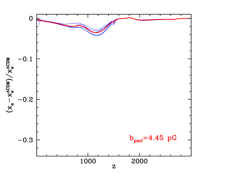
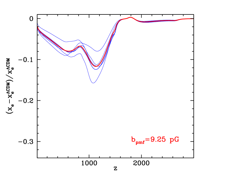
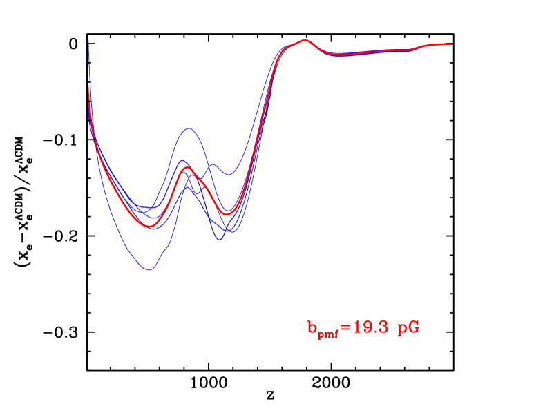
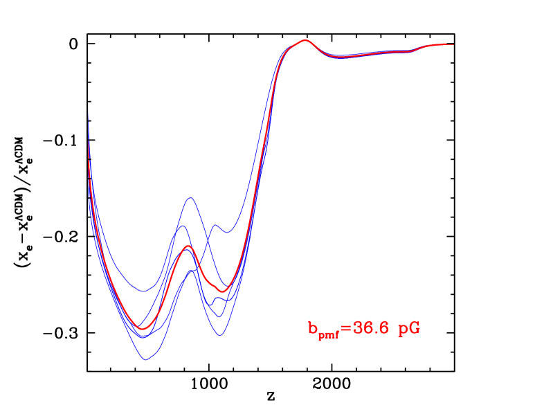
Figure 4: Relative differences in the ionization histories $x_{e}(z)$ with respect to the reference $\Lambda$CDM model obtained from MHD simulations with total $z=10$ comoving magnetic field strength of 4.45 pG (top-left), 9.25 pG (top-right), 19.3 pG (bottom-left) and 36.6 pG (bottom-right). The present-day field strength values are approximately 17% lower, while the corresponding values at recombination are given in Table 3 and are a factor of 10 larger. The blue lines are the results from the 5 realizations at each $b_{\rm pmf}$ with the mean ionization history shown in red.

For the computation of the average ionized fraction $\bar{x}_{e}(z)$ we use a suite of detailed MHD simulations. Magnetohydrodynamic evolution of the magnetized baryon fluid is computed with a modified version of the publicly available code ENZO Bryan et al. (2014). The simulations assume a non-helical magnetic field with Batchelor spectrum. The evolution of local electron density is computed using a private cosmic recombination code. This code mimics the code RECFAST Seager et al. (1999); Wong et al. (2008); Seager et al. (2011) and reproduces the results of RECFAST in a homogeneous non-magnetized Universe to better than the $0.5\%$ accuracy. The private recombination code accounts for the mixing of Lyman-$\alpha$ photons which is important at small magnetic field strengths (i.e. small coherence scales). In our simulation we assume $100\%$ mixing of Lyman-$\alpha$ photons between different regions, inspired by the results of detailed Monte-Carlo simulations of Lyman-$\alpha$ photon transport Jedamzik et al. (2023). The evolution of the baryon gas takes into account the drag force exerted by the CMB photons on moving baryons. Local speed of sound and drag force are computed from the local ionized fraction. A detailed investigation of Lyman-$\alpha$ photon loss due to peculiar motions of the baryons establishes that such effects may be approximately neglected as they influence $\bar{x}_{e}$ at a less than $1\%$ level. The simulations also take into account hydrodynamic heating of baryons by dissipation of magnetic fields. The relatively small simulations of $256^{3}$ zones are computationally demanding and require about $2$ CPU-years. A detailed analysis makes sure that the most relevant modes influencing $\bar{x}_{e}(z)$ are simulated. However, the smallness of the simulation volume results in significant realization variance. We discuss this issue in the next section. Some residual dependence on unsimulated UV modes still remains.

$b_{\rm pmf}$	$b_{\rm bmf}^{\rm rec}$	$B_{1{\rm Mpc}}$
$4.45\times 10^{-3}$ nG	$5.45\times 10^{-2}$ nG	$1.68\times 10^{-10}$ nG
$9.25\times 10^{-3}$ nG	$1.04\times 10^{-1}$ nG	$1.90\times 10^{-9}$ nG
$1.93\times 10^{-2}$ nG	$1.89\times 10^{-1}$ nG	$2.15\times 10^{-8}$ nG
$3.66\times 10^{-2}$ nG	$3.65\times 10^{-1}$ nG	$2.44\times 10^{-7}$ nG

Table 3: Total comoving magnetic field strengths at $z=10$, $b_{\rm pmf}$, for the MHD simulations used in this paper, and the corresponding total comoving field strengths $b_{\rm pmf}^{\rm rec}$ evaluated at the peak of the visibility function ($z\approx 1090$). Also shown are the values of $B_{1{\rm Mpc}}$ commonly used in the literature on CMB anisotropy constraints on PMF.

Final field strength at $z=10$, $b_{\rm pmf}$, is computed by independent simulations taking into account those modes which dominate the final field. The corresponding field strengths at recombination ($z\approx 1090$) are approximately a factor of ten larger and are provided in Table 3. This is due to the additional damping that takes place shortly after recombination when the plasma transitions from highly viscous to turbulent state. Between $z\approx 100$ and $z=0$, the damping is logarithmic Banerjee and Jedamzik (2004), which means the present-day PMF is about 17% smaller than $b_{\rm pmf}$, but still comparable to it. Constraints on PMFs from CMB anisotropies are often presented in terms of the field strength smoothed over a $1$ Mpc size region, $B_{1{\rm Mpc}}$, and the magnetic spectrum index $n_{B}$ Paoletti and Finelli (2011); Ade et al. (2016); Zucca et al. (2017). For the Batchelor spectrum, $n_{B}=2$ (in the notation where the scale-invariant spectrum has $n_{B}=-3$), making $B_{1{\rm Mpc}}$ negligible compared to $b_{\rm pmf}^{\rm rec}$.

IV.2 Obtaining ionization histories for general values of PMF strengths and cosmological parameters

The MHD simulations provide us with the difference in $x_{e}(z)$ relative to a fiducial $\Lambda$CDM model ionization history between $z=4500$ and $z=10$ for 4 values of $z=10$ comoving PMF strengths: $b_{\rm pmf}=4.45$ pico-Gauss (pG), $9.25$ pG, $19.3$ pG and $36.6$ pG, with cosmological parameters at their fiducial values $\bf{\Omega}^{\rm fid}$. The relative difference is defined as

$$\Delta_{e}(z,{\bf\Omega}^{\rm fid})={x_{e}^{\rm pmf}(z,{\bf\Omega}^{\rm fid})-x_{e}^{\rm\Lambda CDM}(z,{\bf\Omega}^{\rm fid})\over x_{e}^{\rm\Lambda CDM}(z,{\bf\Omega}^{\rm fid})}.$$ (1)

We then use linear interpolation to obtain $\Delta_{e}(z,{\bf\Omega}^{\rm fid})$ for other values of $b_{\rm pmf}$, with $\Delta_{e}(z,{\bf\Omega}^{\rm fid})=0$ for $b_{\rm pmf}=0$ by definition. We assume that the dependence of $x_{e}^{\rm PMF}(z)$ on the cosmological parameters is largely the same as in $\Lambda$CDM, implying that $\Delta_{e}(z)$ is effectively independent of cosmological parameters for models that are reasonably close to $\Lambda$CDM. With than assumption, we obtain $x_{e}^{\rm pmf}(z)$ for a given vector of cosmological parameters $\bf{\Omega}$ as

$$x_{e}^{\rm pmf}(z,{\bf\Omega})=x_{e}^{\rm\Lambda CDM}(z,{\bf\Omega})[1+\Delta_{e}(z,\bf{\Omega}^{\rm fid})],$$ (2)

and implement it in RECFAST inside CAMB that is used with Cobaya Torrado and Lewis (2021, 2019) to constrain the parameters.

IV.3 Using randomly generated ensemble of ionization histories instead of the mean $x_{e}(z)$

For the main results of this paper, we used the mean ionization histories obtained by averaging over 5 MHD realizations. Doing so does not account for the large variance in $\Delta_{e}(z)$ from realization to realization clearly seen in Fig. 4. Strictly speaking, the constraints we derive on $b_{\rm pmf}$ and the cosmological parameters should account for the theoretical uncertainty in $\Delta_{e}(z)$, which in our case is dominated by the sample variance of the MHD-derived results. To investigate the impact of accounting for the sample variance in $\Delta_{e}(z)$, we ran MCMC chains for one data combination, Planck+DESI+PP+$M_{b}$, using ionization histories randomly generated from a Gaussian distribution with the mean and covariance derived from the 5 MHD realizations at each PMF strength.

Figure 5: $\Delta_{e}(z)$ generated randomly from a Gaussian distribution a mean and covariance corresponding to $b_{\rm pmf}=10$ pG. The figure shows 20 random histories in green and the mean in blue.

The ensemble of realizations was generated as follows. Let vector ${\bf x}=\{x_{i}\}$ represent $\Delta_{e}(z_{i})$ at a set of discrete values of redshift $z_{i}$. For a given $b_{\rm pmf}$, we have 5 realizations of ${\bf x}$ from which we can compute the mean, $\langle{\bf x}\rangle$ and the covariance $C\equiv\langle({\bf x}-\langle{\bf x}\rangle)({\bf x}-\langle{\bf x}\rangle)^{T}\rangle$.

To generate a random vector ${\bf y}$ from a Gaussian distribution of covariance $C$ and mean $\langle{\bf x}\rangle$, we first use the Singlular Value Decomposition (SVD) method to decompose the covariance into $C=UWV^{T}$, where $U$ and $V$ are orthogonal matrices and $W$ is a diagonal matrix of singular values of $C$. For a symmetrical matrix $C$, such as our covariance, $U=V$ and the elements of $W$ are the eigenvalues of $C$. Next, we consider a vector ${\bf g}$ drawn from a Gaussian distribution of zero mean and unit covariance, i.e. $\langle{\bf g}\rangle=0$ and $\langle{\bf g}{\bf g}^{T}\rangle=\mathbb{I}$, and build our random vector as ${\bf y}=\langle{\bf x}\rangle+L{\bf g}$, where $L=U\sqrt{W}$. One can readily check that $\langle{\bf y}\rangle=\langle{\bf x}\rangle$, and $\langle({\bf y}-\langle{\bf y}\rangle)({\bf y}-\langle{\bf y}\rangle)^{T}\rangle=\langle L{\bf g}{\bf g}^{T}L^{T}\rangle=L\langle{\bf g}{\bf g}^{T}\rangle L^{T}=UWU^{T}=C$. Thus, the random vector ${\bf y}$ has the desired mean and covariance. In practice, only a handful of eigenvalues have non-negligible values, and thus only a small number of eigenvectors of $C$ (or rows of matrix $L$), corresponding to the largest eigenvalues, need to be stored to accurately generate ${\bf y}$.

The mean and covariance for a given $b_{\rm pmf}$ are obtained by linearly interpolating over the means and covariances at 4 $b_{\rm pmf}$ values available from MHD simulations. Fig. 5 shows a collection of randomly generated $\Delta_{e}(z)$ corresponding to $b_{\rm pmf}=10$ pG.

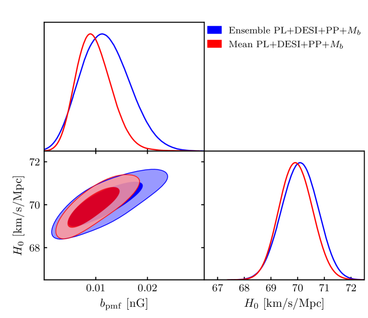
Figure 6: The marginalized $68$% and $95$% CL comparing using the mean vs randomly generated $x_{e}(z)$ when fitting to PL+DESI+PP+$M_{b}$.

Fig. 6 compares posteriors of $b_{\rm pmf}$ and $H_{0}$ obtained by fitting an ensemble of randomly generated $x_{e}(z)$ using the above method vs using the mean $x_{e}(z)$ as in the main text of the paper for PL+DESI+PP+$M_{b}$. As expected, the posteriors are generally wider, especially for $b_{\rm pmf}$, but the differences in constraints on cosmological parameters, including $H_{0}$, are minor. We obtain $b_{\rm pmf}=0.012\pm 0.0044$ nG from the ensemble-based MCMC, compared to $b_{\rm pmf}=0.0096\pm 0.0032$ nG we obtained from the same data combination while using the mean $x_{e}(z)$, corresponding to a 37% increase in uncertainty, and roughly the same statistical significance of $b_{\rm pmf}$ detection. The corresponding values of the Hubble constant were $H_{0}=70.08\pm 0.63$ and $H_{0}=69.93\pm 0.58$ km/s/Mpc for the ensemble-based and the mean-based runs, respectively. The convergence of the ensemble-based MCMC runs is very slow, which is why most of our results are based on using the mean ionization histories. As more MHD runs, or runs using larger simulation boxes become available, the uncertainty around the mean will decrease and the difference between the two methods should disappear, and the MCMC convergence should improve.

IV.4 Datasets

Our datasets included the $\ell>30$ CMB temperature (TT), polarization (EE) and cross-correlation (TE) angular spectra, $C^{\rm TT}_{\ell}$, $C^{\rm EE}_{\ell}$ and $C^{\rm TE}_{\ell}$, as implemented in the Planck PR4 CamSpec (NPIPE) likelihood Rosenberg et al. (2022), the Planck 2018 baseline $\ell<30$ TT and EE likelihoods Aghanim et al. (2020), and the Planck PR4 CMB lensing likelihood Carron et al. (2022). In addition, we used the 12 BAO measurements at 7 effective redshifts from the DESI Year 1 release Adame et al. (2024), and the Pantheon+ (PP) SN dataset Brout et al. (2022) calibrated using the brightness magnitude $M_{b}=-19.253\pm 0.027$ from the cosmic distance ladder measurement by the SH0ES collaboration Riess et al. (2022a). We also use the high-resolution CMB TT, TE, EE spectra from the 2022 release of the South Pole Telescope 3G (SPT-3G) experiment Balkenhol et al. (2023) and from the 4th data release of the Atacama Cosmology Telescope experiment (ACT-DR4) Aiola et al. (2020). We use Cobaya Torrado and Lewis (2021, 2019) to perform the MCMC analysis.

Acknowledgments. We thank Andrei Frolov and Hamid Mirpoorian for valuable discussions and technical assistance. This research was enabled in part by support provided by the BC DRI Group and the Digital Research Alliance of Canada (alliancecan.ca). K.J. is supported in part by ANR grant COSMAG. L.P. is supported in part by the National Sciences and Engineering Research Council (NSERC) of Canada. T.A. is in part supported by the U.S. Department of Energy SLAC Contract No.DE-AC02-76SF00515.

Appendix A Supplemental Material

A.1 Parameter tables

$\Lambda$CDM	PL	DESI	DESI+$\theta_{\mathrm{CMB}}$	PL+DESI	PL+DESI+PP	PL+DESI+PP+$M_{b}$
$\log(10^{10}A_{\mathrm{s}})$	$3.038\pm 0.014$	-	-	$3.045\pm 0.014$	$3.043\pm 0.014$	$3.052\pm 0.014$
$n_{\mathrm{s}}$	$0.9635\pm 0.0040$	-	-	$0.9671\pm 0.0036$	$0.9663\pm 0.0036$	$0.9702\pm 0.0035$
$100\theta_{\mathrm{MC}}$	$1.04075\pm 0.00025$	-	-	$1.04092\pm 0.00024$	$1.04089\pm 0.00024$	$1.04111\pm 0.00024$
$\Omega_{\mathrm{b}}h^{2}$	$0.02218\pm 0.00013$	-	-	$0.02228\pm 0.00013$	$0.02226\pm 0.00012$	$0.02242\pm 0.00012$
$\Omega_{\mathrm{c}}h^{2}$	$0.1197\pm 0.0011$	-	-	$0.11829\pm 0.00081$	$0.11859\pm 0.00078$	$0.11707\pm 0.00075$
$\tau_{\mathrm{reio}}$	$0.0526\pm 0.0071$	-	-	$0.0573\pm 0.0072$	$0.0563\pm 0.0070$	$0.0618\pm 0.0073$
$H_{0}{\rm[km/s/Mpc]}$	$67.22\pm 0.47$	-	-	$67.88\pm 0.37$	$67.74\pm 0.35$	$68.49\pm 0.34$
$\Omega_{\mathrm{m}}$	$0.3156\pm 0.0065$	$0.295\pm 0.014$	$0.295\pm 0.008$	$0.3066\pm 0.0049$	$0.3084\pm 0.0047$	$0.2988\pm 0.0044$
$\Omega_{\mathrm{m}}h^{2}$	$0.14257\pm 0.00099$	-	-	$0.14122\pm 0.00077$	$0.14150\pm 0.00075$	$0.14014\pm 0.00072$
$\sigma_{8}$	$0.8078\pm 0.0055$	-	-	$0.8066\pm 0.0056$	$0.8069\pm 0.0056$	$0.8058\pm 0.0058$
$S_{8}$	$0.828\pm 0.011$	-	-	$0.8154\pm 0.0090$	$0.8181\pm 0.0089$	$0.8042\pm 0.0086$
$r_{\mathrm{drag}}h\ {\rm[Mpc]}$	$99.07\pm 0.81$	$101.89\pm 1.25$	$101.89\pm 1.01$	$100.22\pm 0.63$	$99.98\pm 0.60$	$101.24\pm 0.59$
$r_{\mathrm{drag}}\ {\rm[Mpc]}$	$147.38\pm 0.24$	-	-	$147.65\pm 0.21$	$147.60\pm 0.21$	$147.82\pm 0.21$
$z_{\rm{drag}}$	$1059.48\pm 0.28$	-	-	$1059.61\pm 0.28$	$1059.58\pm 0.27$	$1059.84\pm 0.27$
$r_{\mathrm{s}}\ {\rm[Mpc]}$	$144.65\pm 0.24$	-	-	$144.95\pm 0.20$	$144.89\pm 0.19$	$145.16\pm 0.19$
$z_{\mathrm{s}}$	$1090.14\pm 0.23$	-	-	$1089.88\pm 0.20$	$1089.93\pm 0.19$	$1089.60\pm 0.18$
$\chi^{2}_{\rm highl}$	$10543.7$	-	-	$10545.6$	$10546.7$	$10549.3$
$\chi^{2}_{\rm lensing}$	$8.51$	-	-	$8.54$	$8.79$	$9.28$
$\chi^{2}_{\rm lowlTT}$	$23.72$	-	-	$22.75$	$22.66$	$22.60$
$\chi^{2}_{\rm lowlEE}$	$395.72$	-	-	$397.02$	$396.39$	$398.75$
$\chi^{2}_{\rm PL}$	$10971.7$	-	-	$10973.9$	$10974.5$	$10979.9$
$\chi^{2}_{\rm DESI}$	-	$14.71$	$12.74$	$16.55$	$15.55$	$13.20$
$\chi^{2}_{\rm PP}$	-	-	-	-	$1404.9$	$1406.8$
$\chi^{2}_{M_{b}}$	-	-	-	-	-	$32.12$
$\chi^{2}_{\rm PL+DESI}$	-	-	-	$10990.4$	$10990.0$	$10,993.1$
$\chi^{2}_{\rm PL+DESI+PP}$	-	-	-	-	$12395.0$	$12399.9$
$\chi^{2}_{{\rm PL+DESI+PP}M_{b}}$	-	-	-	-	-	$12432.0$

Table 4: The mean values and standard deviations of the primary and selected derived parameters of the $\Lambda$CDM model fit to combinations of Planck (PL), DESI BAO, angular size of the CMB acoustic scale $\theta_{\mathrm{CMB}}$, and uncalibrated Pantheon+ (PP) SN, along with the best fit $\chi^{2}$ values.

$b\Lambda$CDM	PL	PL+DESI	PL+DESI+PP	PL+DESI+PP+$M_{b}$
$b_{\mathrm{pmf}}\ {\rm[nG]}$	$0.0029\pm 0.0021$	$0.0042\pm 0.0023$	$0.0038\pm 0.0021$	$0.0096\pm 0.0032$
$\log(10^{10}A_{\mathrm{s}})$	$3.041\pm 0.014$	$3.048\pm 0.014$	$3.047\pm 0.014$	$3.054\pm 0.014$
$n_{\mathrm{s}}$	$0.9668\pm 0.0050$	$0.9714\pm 0.0045$	$0.9700\pm 0.0044$	$0.9791\pm 0.0042$
$100\theta_{\mathrm{MC}}$	$1.04201\pm 0.00124$	$1.0429\pm 0.00149$	$1.04260\pm 0.00134$	$1.0467\pm 0.0019$
$\Omega_{\mathrm{b}}h^{2}$	$0.02233\pm 0.00018$	$0.02248\pm 0.00017$	$0.02244\pm 0.00017$	$0.02279\pm 0.00016$
$\Omega_{\mathrm{c}}h^{2}$	$0.1198\pm 0.0010$	$0.11882\pm 0.00092$	$0.11906\pm 0.00088$	$0.1192\pm 0.0010$
$\tau_{\mathrm{reio}}$	$0.0535\pm 0.0072$	$0.0573\pm 0.0071$	$0.0565\pm 0.0070$	$0.0589\pm 0.0073$
$H_{0}{\rm[km/s/Mpc]}$	$67.75\pm 0.68$	$68.52\pm 0.57$	$68.29\pm 0.53$	$69.93\pm 0.58$
$\Omega_{\mathrm{m}}$	$0.3112\pm 0.0075$	$0.3024\pm 0.0055$	$0.3048\pm 0.0052$	$0.2917\pm 0.0048$
$\Omega_{\mathrm{m}}h^{2}$	$0.1428\pm 0.0010$	$0.14195\pm 0.00094$	$0.14214\pm 0.00089$	$0.1426\pm 0.0011$
$\sigma_{8}$	$0.8111\pm 0.0063$	$0.8122\pm 0.0068$	$0.8119\pm 0.0066$	$0.8210\pm 0.0074$
$S_{8}$	$0.826\pm 0.011$	$0.8154\pm 0.0090$	$0.8184\pm 0.0088$	$0.8095\pm 0.0087$
$r_{\mathrm{drag}}h\ {\rm[Mpc]}$	$99.62\pm 0.97$	$100.77\pm 0.73$	$100.45\pm 0.69$	$102.24\pm 0.68$
$r_{\mathrm{drag}}\ {\rm[Mpc]}$	$147.05\pm 0.37$	$147.06\pm 0.45$	$147.08\pm 0.41$	$146.20\pm 0.53$
$z_{\rm{drag}}$	$1061.4\pm 1.79$	$1062.6\pm 2.14$	$1062.2\pm 1.93$	$1068.0\pm 2.7$
$r_{\mathrm{s}}\ {\rm[Mpc]}$	$144.36\pm 0.35$	$144.40\pm 0.43$	$144.41\pm 0.39$	$143.59\pm 0.52$
$z_{\mathrm{s}}$	$1091.82\pm 1.65$	$1092.7\pm 2.11$	$1092.3\pm 1.89$	$1097.9\pm 2.8$
$\chi^{2}_{\rm highl}$	$10544$	$10546.1$	$10544.8$	$10551.2$
$\chi^{2}_{\rm lensing}$	$8.62$	$8.56$	$8.59$	$9.32$
$\chi^{2}_{\rm lowlTT}$	$21.66$	$20.69$	$20.71$	$20.65$
$\chi^{2}_{\rm lowlEE}$	$395.69$	$396.21$	$396.75$	$396.46$
$\chi^{2}_{\rm PL}$	$10970$	$10971.6$	$10970.9$	$10977.6$
$\chi^{2}_{\rm DESI}$	-	$14.07$	$15.14$	$12.91$
$\chi^{2}_{\rm PP}$	-	-	$1405.13$	$1408.34$
$\chi^{2}_{M_{b}}$	-	-	-	$17.90$
$\chi^{2}_{\rm PL+DESI}$	-	$10985.7$	$10986.04$	$10990.51$
$\chi^{2}_{\rm PL+DESI+PP}$	-	$10985.7$	$12391.17$	$12398.85$
$\chi^{2}_{{\rm PL+DESI+PP}M_{b}}$	-	-	-	$12416.75$

Table 5: The mean values and standard deviations uncertainties of the primary and selected derived parameters of the $b\Lambda$CDM model fit to combinations of Planck (PL), DESI BAO, uncalibrated Pantheon+ (PP) SN, PP calibrated using the SH0ES value of the intrinsic SN brightness (PP+$M_{b}$), along with the best fit $\chi^{2}$ values.

	$\Lambda$CDM PL+DESI+		$b\Lambda$CDM PL+DESI+		$b\Lambda$CDM PL+DESI+PP+$M_{b}$+
	ACT	SPT	ACT	SPT	ACT	SPT
$b_{\mathrm{pmf}}\ {\rm[nG]}$	-	-	$0.0030\pm 0.0017$	$0.0036\pm 0.0019$	$0.0064\pm 0.0021$	$0.0074\pm 0.0024$
$\log(10^{10}A_{\mathrm{s}})$	$3.051\pm 0.013$	$3.042\pm 0.013$	$3.055\pm 0.014$	$3.046\pm 0.014$	$3.062\pm 0.014$	$3.053\pm 0.014$
$n_{\mathrm{s}}$	$0.9702\pm 0.0032$	$0.9670\pm 0.0035$	$0.9734\pm 0.0038$	$0.9708\pm 0.0041$	$0.9797\pm 0.0041$	$0.9777\pm 0.0042$
$100\theta_{\mathrm{MC}}$	$1.04106\pm 0.00023$	$1.04084\pm 0.00023$	$1.04227\pm 0.00095$	$1.04236\pm 0.00115$	$1.0446\pm 0.00160$	$1.0452\pm 0.00175$
$\Omega_{\mathrm{b}}h^{2}$	$0.02229\pm 0.00011$	$0.02227\pm 0.00011$	$0.02245\pm 0.00015$	$0.02246\pm 0.00016$	$0.02271\pm 0.00014$	$0.02273\pm 0.00015$
$\Omega_{\mathrm{c}}h^{2}$	$0.11820\pm 0.00080$	$0.11827\pm 0.00080$	$0.11850\pm 0.00082$	$0.11863\pm 0.00085$	$0.11831\pm 0.00094$	$0.11862\pm 0.00099$
$\tau_{\mathrm{reio}}$	$0.0564\pm 0.0070$	$0.0557\pm 0.0069$	$0.0570\pm 0.0071$	$0.0560\pm 0.0071$	$0.0596\pm 0.0073$	$0.0588\pm 0.0073$
$H_{0}{\rm[km/s/Mpc]}$	$67.95\pm 0.35$	$67.85\pm 0.35$	$68.39\pm 0.47$	$68.38\pm 0.50$	$69.47\pm 0.51$	$69.56\pm 0.54$
$\Omega_{\mathrm{m}}$	$0.3057\pm 0.0047$	$0.3068\pm 0.0047$	$0.3028\pm 0.0050$	$0.3032\pm 0.0052$	$0.2936\pm 0.0046$	$0.2935\pm 0.0046$
$\Omega_{\mathrm{m}}h^{2}$	$0.14114\pm 0.00077$	$0.14118\pm 0.00077$	$0.14160\pm 0.00082$	$0.14174\pm 0.00086$	$0.14166\pm 0.00097$	$0.1420\pm 0.0010$
$\sigma_{8}$	$0.8101\pm 0.0054$	$0.8056\pm 0.0054$	$0.8141\pm 0.0061$	$0.8100\pm 0.0064$	$0.8194\pm 0.0070$	$0.8168\pm 0.0071$
$S_{8}$	$0.8177\pm 0.0089$	$0.8146\pm 0.0088$	$0.8178\pm 0.0088$	$0.8142\pm 0.0089$	$0.8105\pm 0.0086$	$0.8079\pm 0.0084$
$r_{\mathrm{drag}}h\ {\rm[Mpc]}$	$100.35\pm 0.62$	$100.19\pm 0.61$	$100.72\pm 0.67$	$100.65\pm 0.69$	$101.97\pm 0.64$	$101.97\pm 0.65$
$r_{\mathrm{drag}}\ {\rm[Mpc]}$	$147.67\pm 0.21$	$147.67\pm 0.21$	$147.27\pm 0.34$	$147.19\pm 0.38$	$146.78\pm 0.46$	$146.59\pm 0.50$
$z_{\rm{drag}}$	$1059.61\pm 0.25$	$1059.58\pm 0.25$	$1061.58\pm 1.43$	$1062.0\pm 1.68$	$1065.0\pm 2.23$	$1066.0\pm 2.44$
$r_{\mathrm{s}}\ {\rm[Mpc]}$	$144.97\pm 0.20$	$144.97\pm 0.20$	$144.60\pm 0.32$	$144.53\pm 0.35$	$144.17\pm 0.45$	$143.98\pm 0.49$
$z_{\mathrm{s}}$	$1089.86\pm 0.18$	$1089.89\pm 0.18$	$1091.57\pm 1.33$	$1092.02\pm 1.60$	$1094.6\pm 2.33$	$1095.7\pm 2.54$
$\chi^{2}_{\rm highl}$	$10546.6$	$10550.6$	$10546$	$10545.6$	$10549.4$	$10553.4$
$\chi^{2}_{\rm lensing}$	$8.35$	$8.89$	$8.36$	$8.78$	$8.60$	$8.68$
$\chi^{2}_{\rm lowlTT}$	$22.74$	$23.03$	$20.41$	$20.90$	$20.60$	$20.19$
$\chi^{2}_{\rm lowlEE}$	$398.04$	$396.023$	$398.04$	$395.78$	$396.86$	$398.99$
$\chi^{2}_{\rm PL}$	$10975.7$	$10978.6$	$10972.8$	$10971.1$	$10975.4$	$10981.2$
$\chi^{2}_{\rm DESI}$	$15.15$	$16.41$	$14.36$	$17.59$	$12.74$	$12.80$
$\chi^{2}_{\rm ACT}$	$242.16$	-	$240.55$	-	$243.12$	-
$\chi^{2}_{\rm SPT}$	-	$1877.4$	-	$1878.5$	-	$1882.2$
$\chi^{2}_{\rm PL+DESI+ACT}$	$11233.0$	-	$11227.7$	-	$11231.3$	-
$\chi^{2}_{\rm PL+DESI+SPT}$	-	$12872.4$	-	$12867.2$	-	12876.2

Table 6: The mean values and standard deviations of the primary and selected derived parameters of the $\Lambda$CDM and the $b\Lambda$CDM models fit to combinations of Planck (PL), DESI BAO, Pantheon+ (PP) SN, SH0ES-calibrated PP (PP+$M_{b}$), ACT DR4 and SPT-3G data, along with the best fit $\chi^{2}$ values.

References

- Aghanim et al. (2020) N. Aghanim et al. (Planck), Astron. Astrophys. 641, A6 (2020), [Erratum: Astron.Astrophys. 652, C4 (2021)], arXiv:1807.06209 [astro-ph.CO] .
- Riess et al. (2022a) A. G. Riess et al., Astrophys. J. Lett. 934, L7 (2022a), arXiv:2112.04510 [astro-ph.CO] .
- Riess et al. (2022b) A. G. Riess, L. Breuval, W. Yuan, S. Casertano, L. M. Macri, J. B. Bowers, D. Scolnic, T. Cantat-Gaudin, R. I. Anderson, and M. C. Reyes, Astrophys. J. 938, 36 (2022b), arXiv:2208.01045 [astro-ph.CO] .
- Freedman et al. (2024) W. L. Freedman, B. F. Madore, I. S. Jang, T. J. Hoyt, A. J. Lee, and K. A. Owens, (2024), arXiv:2408.06153 [astro-ph.CO] .
- Abbott et al. (2023) T. M. C. Abbott et al. (Kilo-Degree Survey, DES), Open J. Astrophys. 6, 2305.17173 (2023), arXiv:2305.17173 [astro-ph.CO] .
- Amon et al. (2022) A. Amon et al. (DES), Phys. Rev. D 105, 023514 (2022), arXiv:2105.13543 [astro-ph.CO] .
- Asgari et al. (2021) M. Asgari et al. (KiDS), Astron. Astrophys. 645, A104 (2021), arXiv:2007.15633 [astro-ph.CO] .
- Brout et al. (2022) D. Brout et al., Astrophys. J. 938, 110 (2022), arXiv:2202.04077 [astro-ph.CO] .
- Abbott et al. (2024) T. M. C. Abbott et al. (DES), Astrophys. J. Lett. 973, L14 (2024), arXiv:2401.02929 [astro-ph.CO] .
- Rubin et al. (2023) D. Rubin et al., (2023), arXiv:2311.12098 [astro-ph.CO] .
- Adame et al. (2024) A. G. Adame et al. (DESI), (2024), arXiv:2404.03002 [astro-ph.CO] .
- Abdalla et al. (2022) E. Abdalla et al., JHEAp 34, 49 (2022), arXiv:2203.06142 [astro-ph.CO] .
- Jedamzik and Abel (2013) K. Jedamzik and T. Abel, JCAP 10, 050 (2013).
- Jedamzik and Pogosian (2020) K. Jedamzik and L. Pogosian, Phys. Rev. Lett. 125, 181302 (2020), arXiv:2004.09487 [astro-ph.CO] .
- Thiele et al. (2021) L. Thiele, Y. Guan, J. C. Hill, A. Kosowsky, and D. N. Spergel, Phys. Rev. D 104, 063535 (2021), arXiv:2105.03003 [astro-ph.CO] .
- Rashkovetskyi et al. (2021) M. Rashkovetskyi, J. B. Muñoz, D. J. Eisenstein, and C. Dvorkin, Phys. Rev. D 104, 103517 (2021), arXiv:2108.02747 [astro-ph.CO] .
- Widrow (2002) L. M. Widrow, Rev. Mod. Phys. 74, 775 (2002), arXiv:astro-ph/0207240 .
- Neronov and Vovk (2010) A. Neronov and I. Vovk, Science 328, 73 (2010), arXiv:1006.3504 [astro-ph.HE] .
- Govoni et al. (2019) F. Govoni, E. Orrù, A. Bonafede, M. Iacobelli, R. Paladino, F. Vazza, M. Murgia, V. Vacca, G. Giovannini, L. Feretti, et al., Science 364, 981 (2019).
- Broderick et al. (2018) A. E. Broderick, P. Tiede, P. Chang, A. Lamberts, C. Pfrommer, E. Puchwein, M. Shalaby, and M. Werhahn, Astrophys. J. 868, 87 (2018), arXiv:1808.02959 [astro-ph.HE] .
- Ade et al. (2016) P. A. R. Ade et al. (Planck), Astron. Astrophys. 594, A19 (2016), arXiv:1502.01594 [astro-ph.CO] .
- Zucca et al. (2017) A. Zucca, Y. Li, and L. Pogosian, Phys. Rev. D 95, 063506 (2017), arXiv:1611.00757 [astro-ph.CO] .
- Jedamzik and Saveliev (2019) K. Jedamzik and A. Saveliev, Phys. Rev. Lett. 123, 021301 (2019), arXiv:1804.06115 [astro-ph.CO] .
- Turner and Widrow (1988) M. S. Turner and L. M. Widrow, Phys. Rev. D37, 2743 (1988).
- Ratra (1992) B. Ratra, Astrophys. J. 391, L1 (1992).
- Durrer and Neronov (2013) R. Durrer and A. Neronov, Astron. Astrophys. Rev. 21, 62 (2013), arXiv:1303.7121 [astro-ph.CO] .
- Vachaspati (1991) T. Vachaspati, Phys. Lett. B265, 258 (1991).
- Vachaspati (2021) T. Vachaspati, Rept. Prog. Phys. 84, 074901 (2021), arXiv:2010.10525 [astro-ph.CO] .
- Wagstaff and Banerjee (2016) J. M. Wagstaff and R. Banerjee, JCAP 01, 002 (2016), arXiv:1409.4223 [astro-ph.CO] .
- Banerjee and Jedamzik (2004) R. Banerjee and K. Jedamzik, Phys. Rev. D 70, 123003 (2004), arXiv:astro-ph/0410032 .
- Hosking and Schekochihin (2021) D. N. Hosking and A. A. Schekochihin, Phys. Rev. X 11, 041005 (2021), arXiv:2012.01393 [physics.flu-dyn] .
- Brandenburg et al. (2015) A. Brandenburg, T. Kahniashvili, and A. G. Tevzadze, Phys. Rev. Lett. 114, 075001 (2015), arXiv:1404.2238 [astro-ph.CO] .
- Zrake (2014) J. Zrake, Astrophys. J. 794, L26 (2014), arXiv:1407.5626 [astro-ph.HE] .
- Zhou et al. (2022) H. Zhou, R. Sharma, and A. Brandenburg, J. Plasma Phys. 88, 905880602 (2022), arXiv:2206.07513 [physics.plasm-ph] .
- Brandenburg et al. (2024) A. Brandenburg, A. Neronov, and F. Vazza, Astron. Astrophys. 687, A186 (2024), arXiv:2401.08569 [astro-ph.CO] .
- Hosking and Schekochihin (2023) D. N. Hosking and A. A. Schekochihin, Nature Commun. 14, 7523 (2023), arXiv:2203.03573 [astro-ph.CO] .
- Lee et al. (2023) N. Lee, Y. Ali-Haïmoud, N. Schöneberg, and V. Poulin, Phys. Rev. Lett. 130, 161003 (2023), arXiv:2212.04494 [astro-ph.CO] .
- Lynch et al. (2024a) G. P. Lynch, L. Knox, and J. Chluba, Phys. Rev. D 110, 063518 (2024a), arXiv:2404.05715 [astro-ph.CO] .
- Lynch et al. (2024b) G. P. Lynch, L. Knox, and J. Chluba, Phys. Rev. D 110, 083538 (2024b), arXiv:2406.10202 [astro-ph.CO] .
- Mirpoorian et al. (2024) S. H. Mirpoorian, K. Jedamzik, and L. Pogosian, (2024), arXiv:2411.16678 [astro-ph.CO] .
- Jedamzik et al. (2023) K. Jedamzik, T. Abel, and Y. Ali-Haimoud, (2023), arXiv:2312.11448 [astro-ph.CO] .
- Lewis et al. (2000) A. Lewis, A. Challinor, and A. Lasenby, Astrophys.J. 538, 473 (2000), arXiv:astro-ph/9911177 [astro-ph] .
- Pogosian et al. (2024) L. Pogosian, G.-B. Zhao, and K. Jedamzik, Astrophys. J. Lett. 973, L13 (2024), arXiv:2405.20306 [astro-ph.CO] .
- Poulin et al. (2024) V. Poulin, T. L. Smith, R. Calderón, and T. Simon, (2024), arXiv:2407.18292 [astro-ph.CO] .
- Galli et al. (2022) S. Galli, L. Pogosian, K. Jedamzik, and L. Balkenhol, Phys. Rev. D 105, 023513 (2022), arXiv:2109.03816 [astro-ph.CO] .
- Aiola et al. (2020) S. Aiola et al. (ACT), JCAP 12, 047 (2020), arXiv:2007.07288 [astro-ph.CO] .
- Balkenhol et al. (2023) L. Balkenhol et al. (SPT-3G), Phys. Rev. D 108, 023510 (2023), arXiv:2212.05642 [astro-ph.CO] .
- Aguirre et al. (2018) J. Aguirre et al. (Simons Observatory), (2018), arXiv:1808.07445 [astro-ph.CO] .
- Abazajian et al. (2019) K. Abazajian et al., (2019), arXiv:1907.04473 [astro-ph.IM] .
- Marinacci et al. (2018) F. Marinacci et al., Mon. Not. Roy. Astron. Soc. 480, 5113 (2018), arXiv:1707.03396 [astro-ph.CO] .
- Banerjee and Jedamzik (2003) R. Banerjee and K. Jedamzik, Phys. Rev. Lett. 91, 251301 (2003), [Erratum: Phys.Rev.Lett. 93, 179901 (2004)], arXiv:astro-ph/0306211 .
- Korochkin et al. (2021) A. Korochkin, O. Kalashev, A. Neronov, and D. Semikoz, Astrophys. J. 906, 116 (2021), arXiv:2007.14331 [astro-ph.CO] .
- Pavičević et al. (2025) M. Pavičević, V. Iršič, M. Viel, J. Bolton, M. G. Haehnelt, S. Martin-Alvarez, E. Puchwein, and P. Ralegankar, (2025), arXiv:2501.06299 [astro-ph.CO] .
- Roper Pol et al. (2022) A. Roper Pol, C. Caprini, A. Neronov, and D. Semikoz, Phys. Rev. D 105, 123502 (2022), arXiv:2201.05630 [astro-ph.CO] .
- Ralegankar (2023) P. Ralegankar, Phys. Rev. Lett. 131, 231002 (2023), arXiv:2303.11861 [astro-ph.CO] .
- Lucca et al. (2024) M. Lucca, J. Chluba, and A. Rotti, Mon. Not. Roy. Astron. Soc. 530, 668 (2024), arXiv:2306.08085 [astro-ph.CO] .
- Bryan et al. (2014) G. L. Bryan et al. (ENZO), Astrophys. J. Suppl. 211, 19 (2014), arXiv:1307.2265 [astro-ph.IM] .
- Seager et al. (1999) S. Seager, D. D. Sasselov, and D. Scott, Astrophys. J. Lett. 523, L1 (1999), arXiv:astro-ph/9909275 .
- Wong et al. (2008) W. Y. Wong, A. Moss, and D. Scott, Mon. Not. Roy. Astron. Soc. 386, 1023 (2008), arXiv:0711.1357 [astro-ph] .
- Seager et al. (2011) S. Seager, D. D. Sasselov, and D. Scott, “RECFAST: Calculate the Recombination History of the Universe,” Astrophysics Source Code Library, record ascl:1106.026 (2011).
- Paoletti and Finelli (2011) D. Paoletti and F. Finelli, Phys.Rev. D83, 123533 (2011), arXiv:1005.0148 [astro-ph.CO] .
- Torrado and Lewis (2021) J. Torrado and A. Lewis, JCAP 05, 057 (2021), arXiv:2005.05290 [astro-ph.IM] .
- Torrado and Lewis (2019) J. Torrado and A. Lewis, “Cobaya: Bayesian analysis in cosmology,” Astrophysics Source Code Library, record ascl:1910.019 (2019).
- Rosenberg et al. (2022) E. Rosenberg, S. Gratton, and G. Efstathiou, Mon. Not. Roy. Astron. Soc. 517, 4620 (2022), arXiv:2205.10869 [astro-ph.CO] .
- Carron et al. (2022) J. Carron, M. Mirmelstein, and A. Lewis, JCAP 09, 039 (2022), arXiv:2206.07773 [astro-ph.CO] .