Pulling Back Theorem for Generalizing the Diagonal Averaging Principle in Symplectic Geometry Mode Decomposition and
Singular Spectrum Analysis

Abstract

The symplectic geometry mode decomposition (SGMD) is a powerful method for analyzing time sequences. The SGMD is based on the upper conversion via embedding and down conversion via diagonal averaging principle (DAP) inherited from the singular spectrum analysis (SSA). However, there are two defects in the DAP: it just hold for the time delay $\tau=1$ in the trajectory matrix and it fails for the time sequence of type-1 with the form $X=\left\{x[n]\right\}^{N}_{n=1}$. In order to overcome these disadvantages, the inverse step for embedding is explored with binary Diophantine equation in number theory. The contributions of this work lie in three aspects: firstly, the pulling back theorem is proposed and proved, which state the general formula for converting the component of trajectory matrix to the component of time sequence for the general representation of time sequence and for any time delay $\tau\geq 1$; secondly a unified framework for decomposing both the deterministic and random time sequences into multiple modes is presented and explained; finally, the guidance of configuring the time delay is suggested, namely the time delay should be selected in a limited range via balancing the efficiency of matrix computation and accuracy of state estimation. It could be expected that the pulling back theorem will help the researchers and engineers to deepen the understanding of the theory and extend the applications of the SGMD and SSA in analyzing time sequences.
Keywords: Time sequence (TS); Symplectic geometry mode decomposition (SGMD); Singular spectrum analysis (SSA); Diagonal averaging principle (DAP); Diophantine equation; Pulling back theorem

1 Introduction

The symplectic geometry mode decomposition (SGMD) is originally proposed by Pan et al. in 2019 [1] for decomposing time sequence (TS) which is also named with time series. The SGMD is a development of symplectic geometry spectral analysis [2, 3] and Takens’ delay-time embedding theorem [4] for analyzing nonlinear signals or time sequences. The SGMD employs the symplectic geometry similarity transform [5] to determine the eigenvalues of the Hamilton matrix and build a series of single components, known as the symplectic geometry components (SGCs). These components together maintain the intrinsic characteristics of the TS involved while minimizing modal confusion. Moreover, the building process effectively eliminates noise [6], demonstrating strong decomposition performance and robustness against noise.

In recent five years, there are active researches about the SGMD, such as Jin et al. [7], Zhang [8], Guo et al. [9, 10], Chen et al. [11], Liu et al. [12], Hao et al. [13], Zhan et al [14], and Xin et al. [15]. Although the researches which demonstrate the merits of the SGMD method are still increasing, there is no doubt about the key principle behind the SGMD. Actually, there are two defects about the formula of diagonal averaging for converting the component of trajectory matrix (CRM) to the component of time sequence (CTS) in the original and various version of improved SGMD:

• it just holds for the time delay $\tau=1$ in the step of constructing the trajectory matrix for embedding;

• it works for the type-1 time sequence denoted by $X=\left\{x[n]\right\}^{N}_{n=1}$ but fails for the type-0 time sequence denoted by $X=\left\{x[n]\right\}^{N-1}_{n=0}$ due to different structures of the trajectory matrix.

In this work, our contributions to the SGMD lies in three aspects in the sense of theory and practice:

• the pulling back theorem is proposed and proved, which state the correct form of the formula for converting the CRM to the CTS for the time sequence $X$ of type-$s$ denoted by $X=\left\{x[n]\right\}^{N-1+s}_{n=s}$ for $s\in\left\{0,1\right\}$ and time delay $\tau\in\mathbb{N}$;

• a unified framework for decomposing both the deterministic and random time sequences into multiple modes is presented and explained;

• the guidance of configuring the time delay is suggested — it should be selected in a limited range with a trade off between the efficiency of matrix computation and accuracy of state estimation.

The contents of this paper are organized as follows: Section 2 copes with the preliminaries about the notations and binary Diophantine equation; Section 3 deals with the general embedding process for generating the trajectory matrix for the time sequence; Section 4 covers the pulling back theorem, which is the key issue of this work; Section 5 is the discussion of the SGMD and the pulling back theorem; finally, the conclusions are summarized in Section 6.

For the convenience of reading, some nomenclatures and notations are give in Table 1.

Table 1: Nomenclatures and notations

Notation	Interpretation
TS	time sequence, also named with time series
CTM	Component of Trajectory Matrix
SGMD	Symplectic Geometry Mode Decomposition
SSA	Singular Spectrum Analysis
SGC	Symplectic Geometric Component
ISGC	Initial Symplectic Geometry Component
$\mathbb{Z}$	set of integers, $\mathbb{Z}=\left\{0,\pm 1,\pm 2,\cdots\right\}$
$\mathbb{Z}^{+}$	set of non-negative integers $\mathbb{Z}^{+}=\left\{0,1,2,\cdots\right\}$
$\mathbb{N}$	set of positive integers $\mathbb{N}=\left\{1,2,3,\cdots\right\}$
$\Omega,\Omega(\alpha_{1},\alpha_{2},\beta_{1},\beta_{2})$	rectangular domain such that $\Omega=\left\{(x,y)\in\mathbb{Z}^{2}:\alpha_{1}\leq x\leq\alpha_{2},\beta_{1}\leq y\leq\beta_{2}\right\}$
$\left\lceil{x}\right\rceil$	ceiling of $x\in\mathbb{R}$, the minimal integer $n\in\mathbb{Z}$ such that $n\geq x$
$\left\lfloor{x}\right\rfloor$	floor of $x\in\mathbb{R}$, the maximal integer $n\in\mathbb{Z}$ such that $n\leq x$
$X=\left\{x[n]\right\}^{N-1+s}_{n=s}$	time sequence of type-$s$ with length $N\in\mathbb{N}$ for $s\in\left\{0,1\right\}$
$X^{(k)}=\left\{x^{(k)}[n]\right\}^{N-1+s}_{n=s}$	the $k$-th CTS of type-$s$ with length $N\in\mathbb{N}$ for $s\in\left\{0,1\right\}$ such that $\displaystyle X=\sum^{r}_{k=1}X^{(k)}$
$\mathbb{R}^{{d}\times{m}}$	set of $d\times m$ matrices, immersion space of trajectory matrices
$(\mathscr{X},{n}_{\mathrm{dof}})$	manifold of time sequence with dimension ${n}_{\mathrm{dof}}$
$\Phi:\mathscr{X}\to\mathbb{R}^{{d}\times{m}}$	embedding mapping for up conversion
$\Phi^{-1}:\mathbb{R}^{{d}\times{m}}\to\mathscr{X}$	pulling back for down conversion, inverse of embedding mapping
$\bm{A}=(A^{i}_{j})_{d\times m}\in\mathbb{R}^{{d}\times{m}}$	$d\times m$ matrix, where $A^{i}_{j}$ is the entry located in the $i$-th row and $j$-th column
$\bm{M}=(M^{i}_{j})_{d\times m}=\Phi(X)$	trajectory matrix such that $M^{i}_{j}=(x[i\tau+j+s])$ for $s\in\left\{0,1\right\}$
$\bm{Z}_{k}=(Z^{i}_{j}(k))_{d\times m}$	the $k$-th CTM of the trajectory matrix $\bm{M}$
$(\bm{Z}_{1},\cdots,\bm{Z}_{r})$	group of $r$ CTMs such that $\displaystyle\mathcal{D}(\bm{M})=\sum^{r}_{k=1}\bm{Z}_{k}$
$(\hat{\bm{Z}}_{1},\cdots,\hat{\bm{Z}}_{\hat{r}})$	group of $\hat{r}$ CTMs after denoising
$\mathcal{D}:\mathbb{R}^{{d}\times{m}}\to\mathbb{R}^{{d}\times{m}}$	matrix decomposition, $\displaystyle\mathcal{D}(\bm{M})=\sum^{r}_{k=1}\bm{Z}_{k}$
$\mathcal{F}:\mathbb{R}^{{d}\times{m}}\to\mathbb{R}^{{d}\times{m}}$	denoising operation in the immersion space, $\displaystyle\sum^{\hat{r}}_{k=1}\hat{\bm{Z}}_{k}=\mathcal{F}\left(\sum^{r}_{i=1}\bm{Z}_{i}\right)$
$\Psi:\mathscr{X}\to\mathscr{X}$	SGMD mapping such that $\Psi=\Phi^{-1}\circ\mathcal{D}\circ\Phi$ without denoising or $\Psi=\Phi^{-1}\circ\mathcal{F}\circ\mathcal{D}\circ\Phi$ with denoising

2 Preliminaries

2.1 Notations

The time sequence $X$ of length $N\in\left\{N\right\}$ can be denoted by $x[n]$ for simplicity. However, there are two types of concrete representations for different computer programming languages:

• type-1 for the Fortran/MATLAB/Octave/…

  $$X=\left\{x[n]:1\leq n\leq N\right\}=\left\langle x[1],x[2],\cdots,x[N]\right\rangle$$

• type-0 for the C/C++/Python/Java/Rust/…

  $$X=\left\{x[n]:0\leq n\leq N-1\right\}=\left\langle x[0],x[1],\cdots,x[N-1]\right\rangle$$

It is trivial to find that the unified formula for these two types can be expressed by

$$X=\left\{x[n]:s\leq n\leq N-1+s\right\}=\left\{x[n]\right\}^{N-1+s}_{n=s}$$ (1)

for $s\in\left\{0,1\right\}$. In signal processing, the time sequence $X=\left\{x[n]\right\}^{N-1+s}_{n=s}$ is usually denoted by $x[n]$ for simplicity. An alternative notation for time sequence in mathematics and physics is $x_{n}$. Moreover, the time sequences are also named by discrete time signals or time series.

The manifold of time sequences $X$ ot type $s\in\left\{0,1\right\}$ is denoted by $(\mathscr{X},{n}_{\mathrm{dof}})$, where ${n}_{\mathrm{dof}}$ is the dimension of the space $\mathscr{X}$. Note that ${n}_{\mathrm{dof}}$ is the freedom of degeree for the dynamic system $x(t)$ for $t\geq t_{0}$ such that

$$x[n]=x(t_{0}+n/f),\quad n\in\mathbb{Z}^{+}$$ (2)

where $f$ is the sampling frequency and $t_{0}$ is the initial time. Usually, the $x[n]$ can be regarded as the sum of the ideal signal ${x}_{\mathrm{ideal}}[n]$ and the noise ${x}_{\mathrm{noise}}[n]$, namely

$$x[n]={x}_{\mathrm{ideal}}[n]+{x}_{\mathrm{noise}}[n],\quad n\in\mathbb{Z}^{+}$$ (3)

2.2 Binary Diophantine Equation

2.2.1 General Case

Suppose $N,d,\tau\in\mathbb{N}$ are positive integers. Suppose that $\alpha_{1},\alpha_{2},\beta_{1},\beta_{2}\in\mathbb{Z}^{+}$ such that $0\leq\alpha_{1}<\alpha_{2}$ and $0\leq\beta_{1}<\beta_{2}$. Let

$$\Omega=\Omega(\alpha_{1},\alpha_{2},\beta_{1},\beta_{2})=\left\{(x,y)\in\mathbb{Z}^{2}:\alpha_{1}\leq x\leq\alpha_{2},\beta_{1}\leq y\leq\beta_{2}\right\}$$ (4)

For the given $n\in\mathbb{Z}^{+}$ and $\tau\in\mathbb{N}$, we have $\operatorname{GCD}(\tau,1)=1$ and $n>\tau\cdot 1-\tau-1=-1$, thus the set of solutions to the Diophantine equation

$$\tau x+y=n+s\tau,\quad\forall n\in\mathbb{Z}^{+}$$ (5)

must be non-empty according to the Theorem 6 and Theorem 7 in Appendix A. For $\forall n\in\mathbb{Z}_{+}$, let

$$G_{s}(n,\tau,\alpha_{1},\alpha_{2},\beta_{1},\beta_{2}) =\left\{(x,y)\in\Omega:x\tau+y=n+s\tau\right\}$$ (6)

for $s\in\left\{0,1\right\}$. The cardinality of $G_{s}(n,\cdots)$ is denoted by $\left|G_{s}(n,\cdots)\right|$. The geometric interpretation of the set $G_{s}(n,\cdots)$ is all of the 2-dim points which satisfy (5) with interger coordinates on the line $x\tau+y=n+s\tau$ and in the rectangle domain $\Omega$. Figure 1 illustrates the scenario intuitively.

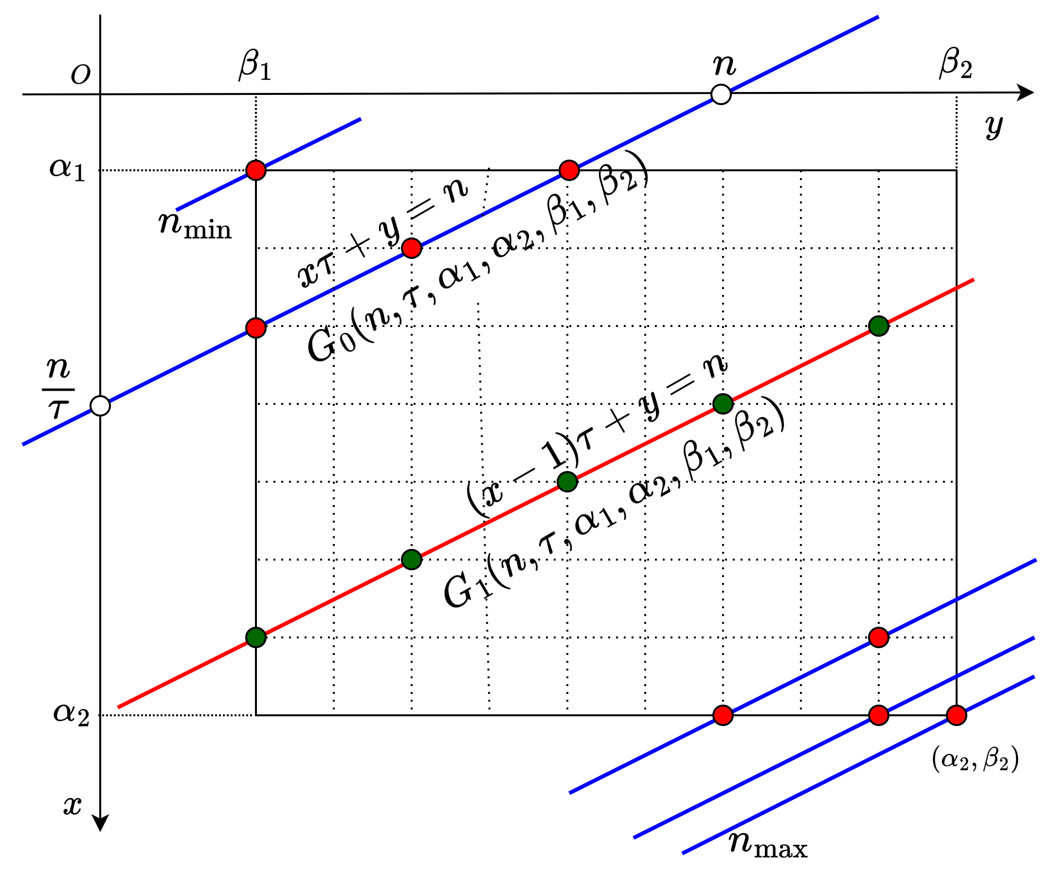
Figure 1: Geometric interpretation of $G_{s}(n,\tau,\alpha_{1},\alpha_{2},\beta_{1},\beta_{2})$

The equation $x\tau+y=n+s\tau$ implies that $y=n+s\tau-x\tau$. Thus $\beta_{1}\leq y\leq\beta_{2}$ implies that

$$\frac{n+s\tau-\beta_{2}}{\tau}\leq x\leq\frac{n+s\tau-\beta_{1}}{\tau}$$ (7)

It is obvious that

$$\max\left(\alpha_{1},\frac{n+s\tau-\beta_{2}}{\tau}\right)\leq x\leq\min\left(\alpha_{2},\frac{n+s\tau-\beta_{1}}{\tau}\right)$$ (8)

For the purpose of finding integer solutions, the $\dfrac{n+s\tau-\beta_{2}}{\tau}$ should be replaced by $\left\lceil{\dfrac{n+s\tau-\beta_{2}}{\tau}}\right\rceil$ and the $\dfrac{n+s\tau-\beta_{1}}{\tau}$ should be replaced by $\left\lfloor{\dfrac{n+s\tau-\beta_{1}}{\tau}}\right\rfloor$, where $\left\lceil{x}\right\rceil$ and $\left\lfloor{x}\right\rfloor$ denote the ceiling and floor of $x\in\mathbb{R}$ respectively. Let

$$\left\{\begin{aligned} {x}_{\mathrm{min}}^{s}(n,\tau,\alpha_{1},\beta_{2})&=\max\left(\alpha_{1},\left\lceil{\frac{n+s\tau-\beta_{2}}{\tau}}\right\rceil\right)\\ {x}_{\mathrm{max}}^{s}(n,\tau,\alpha_{2},\beta_{1})&=\min\left(\alpha_{2},\left\lfloor{\frac{n+s\tau-\beta_{1}}{\tau}}\right\rfloor\right)\end{aligned}\right.$$ (9)

for $s\in\left\{0,1\right\}$, then it is easy to prove the following theorem according to (8) and (9).

Theorem  1.

For the constrained Diophantine equation

$$\tau x+y=n+s\tau,\quad(x,y)\in\Omega,s\in\left\{0,1\right\}$$ (10)

the set of its solutions can be written by

$$G_{s}(n,\tau,\alpha_{1},\alpha_{2},\beta_{1},\beta_{2})=\left\{(x,n-x\tau):{x}_{\mathrm{min}}^{s}(n,\tau,\alpha_{1},\beta_{2})\leq x\leq{x}_{\mathrm{max}}^{s}(n,\tau,\alpha_{2},\beta_{1})\right\}$$ (11)

and the number of solutions is

$$\left|G_{s}(n,\tau,\alpha_{1},\alpha_{2},\beta_{1},\beta_{2})\right|={x}_{\mathrm{max}}^{s}(n,\tau,\alpha_{2},\beta_{1})-{x}_{\mathrm{min}}^{s}(n,\tau,\alpha_{1},\beta_{2})+1.$$ (12)

2.2.2 Special Cases

There are some typical special cases about the structure of $G_{s}(n,\tau,\alpha_{1},\alpha_{2},\beta_{1},\beta_{2})$ for $s\in\left\{0,1\right\}$, $(\alpha_{1},\alpha_{2})\in\left\{(0,d-1),(1,d)\right\}$ and $(\beta_{1},\beta_{2})\in\left\{(0,m-1),(1,m)\right\}$ because of the way of representation of time sequences and coding with concrete computer programming languages.

A. Case of $(\alpha_{1},\alpha_{2},\beta_{1},\beta_{2})=(0,d-1,0,m-1)$

Particularly, for $d,m\in\mathbb{N}$ and $(\alpha_{1},\alpha_{2},\beta_{1},\beta_{2})=(0,d-1,0,m-1)$, we have

$$\left\{\begin{aligned} G_{0}(n,\tau,0,d-1,0,m-1)&=\left\{(x,n-x\tau):{x}^{\mathrm{0}}_{\mathrm{min}}(n,\tau,0,m-1)\leq x\leq{x}^{\mathrm{0}}_{\mathrm{max}}(n,\tau,d-1,0)\right\}\\ \left|G_{0}(n,\tau,0,d-1,0,m-1)\right|&={x}^{\mathrm{0}}_{\mathrm{max}}(n,\tau,d-1,0)-{x}^{\mathrm{0}}_{\mathrm{min}}(n,\tau,0,m-1)+1\end{aligned}\right.$$ (13)

As an illustration, for the parameter configuration $(N,\tau,d,m)=(27,3,7,9)$ and $(\alpha_{2},\alpha_{2},\beta_{1},\beta_{2})=(0,6,0,8)$, we can obtain

$$\left\{\begin{aligned} &{x}^{\mathrm{0}}_{\mathrm{min}}(n,3,0,8)=\max\left(0,\left\lceil{\frac{n-8}{3}}\right\rceil\right)\\ &{x}^{\mathrm{0}}_{\mathrm{max}}(n,3,6,0)=\min\left(6,\left\lfloor{\frac{n}{3}}\right\rfloor\right)\\ \end{aligned}\right.$$ (14)

and

$$G_{0}(n,3,0,6,0,8)=\left\{(x,n-3x):{x}^{\mathrm{0}}_{\mathrm{min}}(n,3,0,8)\leq x\leq{x}^{\mathrm{0}}_{\mathrm{max}}(n,3,6,0)\right\}$$ (15)

The structure of $G_{0}(n,\tau,0,d-1,0,m-1)=G_{0}(n,3,0,6,0,8)$ is listed in Table 2.

Table 2: Structure of $G_{0}=\left\{(x,n-3x):{x}^{\mathrm{0}}_{\mathrm{min}}\leq x\leq{x}^{\mathrm{0}}_{\mathrm{max}}\right\}$ for $N=27$, $\tau=3$, $d=7$, $m=9$, ${x}^{\mathrm{0}}_{\mathrm{min}}=\max\left(0,\left\lceil{\frac{n-8}{3}}\right\rceil\right)$ and ${x}^{\mathrm{0}}_{\mathrm{max}}=\min\left(6,\left\lfloor{\frac{n}{3}}\right\rfloor\right)$

$n$	${x}^{\mathrm{0}}_{\mathrm{min}}$	${x}^{\mathrm{0}}_{\mathrm{max}}$	$G_{0}$	$\left|G_{0}\right|$
$0$	$0$	$0$	$\left\{(0,0)\right\}$	$1$
$1$	$0$	$0$	$\left\{(0,1)\right\}$	$1$
$2$	$0$	$0$	$\left\{(0,2)\right\}$	$1$
$3$	$0$	$1$	$\left\{(0,3),(1,0)\right\}$	$2$
$4$	$0$	$1$	$\left\{(0,4),(1,1)\right\}$	$2$
$5$	$0$	$1$	$\left\{(0,5),(1,2)\right\}$	$2$
$6$	$0$	$2$	$\left\{(0,5),(1,2),(2,0)\right\}$	$3$
$7$	$0$	$2$	$\left\{(0,7),(1,4),(2,1)\right\}$	$3$
$8$	$0$	$2$	$\left\{(0,8),(1,5),(2,2)\right\}$	$3$
$9$	$1$	$3$	$\left\{(1,6),(2,3),(3,0)\right\}$	$3$
$10$	$1$	$3$	$\left\{(1,7),(2,4),(3,1)\right\}$	$3$
$11$	$1$	$3$	$\left\{(1,8),(2,5),(3,2)\right\}$	$3$
$12$	$2$	$4$	$\left\{(2,6),(3,3),(4,0)\right\}$	$3$
$13$	$2$	$4$	$\left\{(2,7),(3,4).(4,1)\right\}$	$3$
$14$	$2$	$4$	$\left\{(2,8),(3,5),(4,2)\right\}$	$3$
$15$	$3$	$5$	$\left\{(3,6),(4,3),(5,0)\right\}$	$3$
$\vdots$	$\vdots$	$\vdots$	$\vdots$	$\vdots$
$26$	$6$	$6$	$\left\{(6,8)\right\}$	$1$

B. Case of $(\alpha_{2},\alpha_{2},\beta_{1},\beta_{2})=(1,d,1,m)$

Particularly, for $d,m\in\mathbb{N}$ and $(\alpha_{1},\alpha_{2},\beta_{1},\beta_{2})=(1,d,1,m)$, we can find that

$$\left\{\begin{aligned} G_{1}(n,\tau,1,d,1,m)&=\left\{(x,n+\tau-x\tau):{x}^{\mathrm{1}}_{\mathrm{min}}(n,\tau,1,m)\leq x\leq{x}^{\mathrm{0}}_{\mathrm{max}}(n,\tau,d,1)\right\}\\ \left|G_{1}(n,\tau,1,d,1,m)\right|&={x}^{\mathrm{1}}_{\mathrm{max}}(n,\tau,d,1)-{x}^{\mathrm{1}}_{\mathrm{min}}(n,\tau,1,m)+1\end{aligned}\right.$$ (16)

Similarly, for the parameter configuration $(N,\tau,d,m)=(27,3,7,9)$ and $(\alpha_{1},\alpha_{2},\beta_{1},\beta_{2})=(1,7,1,9)$, we immediately have

$$\left\{\begin{aligned} &{x}^{\mathrm{1}}_{\mathrm{min}}(n,3,1,9)=\max\left(1,\left\lceil{\frac{n-6}{3}}\right\rceil\right)\\ &{x}^{\mathrm{1}}_{\mathrm{max}}(n,3,7,1)=\min\left(7,\left\lfloor{\frac{n+2}{3}}\right\rfloor\right)\\ &G_{1}(n,3,1,7,1,9)=\left\{(x,n+3-3x):{x}^{\mathrm{1}}_{\mathrm{min}}\leq x\leq{x}^{\mathrm{1}}_{\mathrm{max}}\right\}\end{aligned}\right.$$ (17)

and the structure of $G_{1}(n,\tau,1,d,1,m)=G_{1}(n,3,1,7,1,9)$ is listed in Table 3.

Table 3: Structure of $G_{1}=\tiny{\left\{(x,n+3-3x):\tiny{{x}^{\mathrm{1}}_{\mathrm{min}}\leq x\leq{x}^{\mathrm{1}}_{\mathrm{max}}}\right\}}$ for $N=27$,$\tau=3$,$d=7$,$m=9$, ${x}^{\mathrm{1}}_{\mathrm{min}}=\max\left(1,\left\lceil{\frac{n-6}{3}}\right\rceil\right)$ and ${x}^{\mathrm{1}}_{\mathrm{max}}=\min\left(7,\left\lfloor{\frac{n+2}{3}}\right\rfloor\right)$.

$n$	${x}^{\mathrm{1}}_{\mathrm{min}}$	${x}^{\mathrm{1}}_{\mathrm{max}}$	$G_{1}$	$\left|G_{1}\right|$
$1$	$1$	$1$	$\left\{(1,1)\right\}$	$1$
$2$	$1$	$1$	$\left\{(1,2)\right\}$	$1$
$3$	$1$	$1$	$\left\{(1,3)\right\}$	$1$
$4$	$1$	$2$	$\left\{(1,4),(2,1)\right\}$	$2$
$5$	$1$	$2$	$\left\{(1,5),(2,2)\right\}$	$2$
$6$	$1$	$2$	$\left\{(1,6),(2,3)\right\}$	$2$
$7$	$1$	$3$	$\left\{(1,7),(2,4),(3,1)\right\}$	$3$
$8$	$1$	$3$	$\left\{(1,8),(2,5),(3,2)\right\}$	$3$
$9$	$1$	$3$	$\left\{(1,9),(2,6),(3,3)\right\}$	$3$
$10$	$2$	$4$	$\left\{(2,7),(3,4),(4,1)\right\}$	$3$
$11$	$2$	$4$	$\left\{(2,8),(3,5),(4,2)\right\}$	$3$
$12$	$2$	$4$	$\left\{(2,9),(3,6),(4,3)\right\}$	$3$
$13$	$3$	$5$	$\left\{(3,7),(4,4).(5,1)\right\}$	$3$
$14$	$3$	$5$	$\left\{(3,8),(4,5),(5,2)\right\}$	$3$
$15$	$3$	$5$	$\left\{(3,9),(4,6),(5,3)\right\}$	$3$
$16$	$4$	$6$	$\left\{(4,7),(5,4),(6,1)\right\}$	$3$
$\vdots$			$\vdots$	$\vdots$
$27$	$7$	$7$	$\left\{(7,9)\right\}$	$1$

C. Case of $(\alpha_{1},\alpha_{2},\beta_{1},\beta_{2})=(1,d,1,m)$ and $\tau=1$

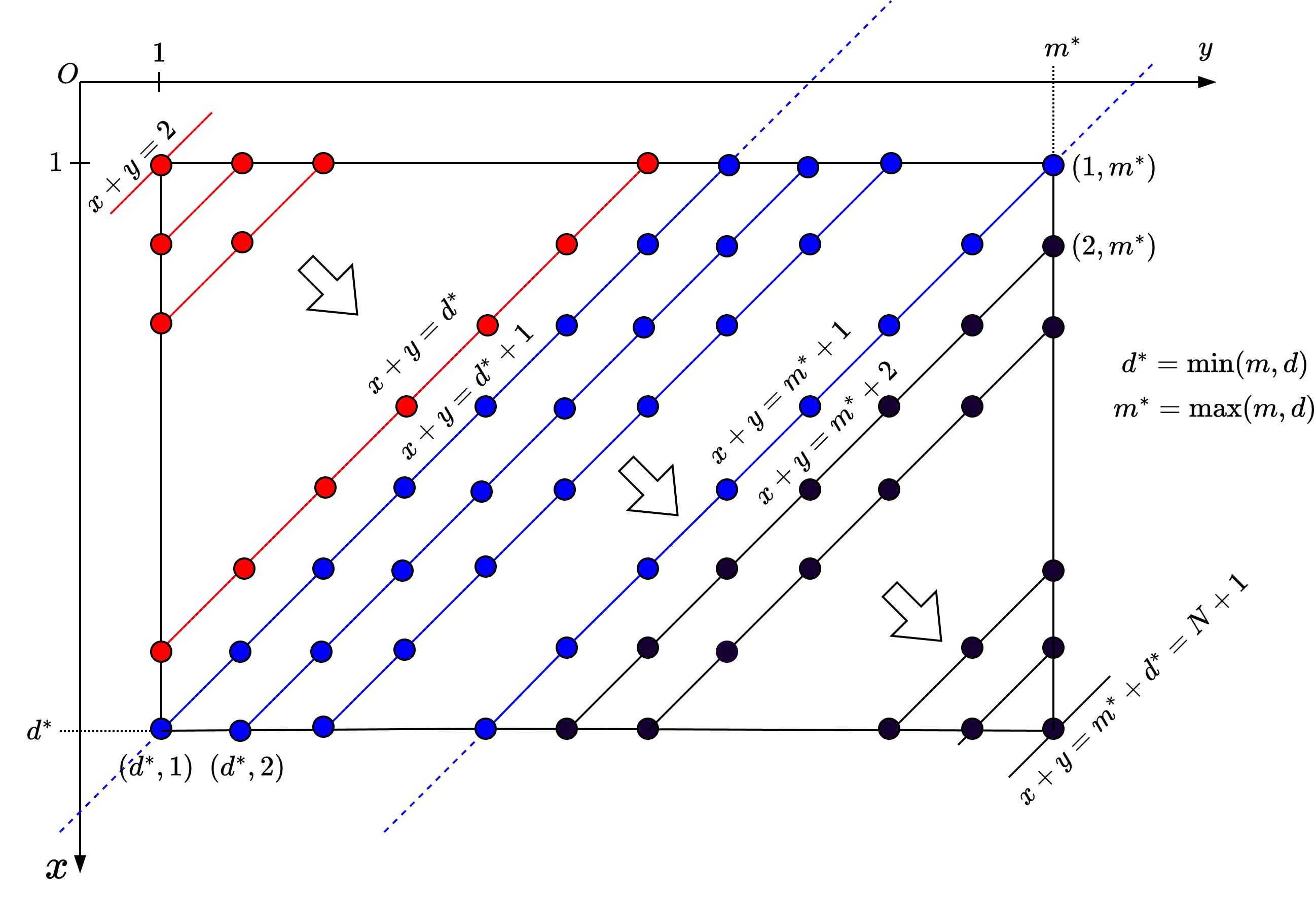
Figure 2: Geometric interpretation of $G_{1}(n,1,1,d,1,m)$

A special case for the $G_{1}(n,\tau,\alpha_{1},\alpha_{2},\beta_{1},\beta_{2})$ such that $(\tau,\alpha_{1},\alpha_{2},\beta_{1},\beta_{2})=(1,1,d,1,m)$ is of interest in the references. Figure 2 illustrates such a scenario. Let

$$d^{*}=\min(d,m),\quad m^{*}=\max(d,m)$$ (18)

then $d+m=\min(d,m)+\max(d,m)=d^{*}+m^{*}$. Thus $N=m+(d-1)\tau=m+d-1=d^{*}+m^{*}-1$ or equivalently $d^{*}+m^{*}=N+1$. For the set

$$G_{1}^{*}(n)=G_{1}(n,1,1,d,1,m)=\left\{(x,n+1-x):{x}^{\mathrm{1}}_{\mathrm{min}}(n,1,1,m)\leq x\leq{x}^{\mathrm{1}}_{\mathrm{max}}(n,1,d,1)\right\},$$ (19)

we can obtain some interesting observations by Figure 2. Actually, we have:

• For $1\leq n<d^{*}$, there are $n$ solutions to the Diophantine equation $\tau x+y=n+\tau$ for $(x,y)\in\Omega(1,d,1,m)$ and $s=1$, thus

  $$\left\{\begin{aligned} &G_{1}^{*}(n)=\left\{(x,n+1-x):1\leq x\leq n\right\}\\ &\left|G_{1}^{*}(n)\right|=n\end{aligned}\right.$$ (20)

  Geometrically, the $G_{1}^{*}(n)$ corresponds to the red points on the red hypotenuse of the equilateral right angled triangle shown in the Figure 2.

• For $d^{*}\leq n\leq m^{*}$, there are always $d^{*}$ solutions to the Diophantine equation $\tau x+y=n+s\tau$ for $(x,y)\in\Omega(1,d,1,m)$, thus

  $$\left\{\begin{aligned} &G_{1}^{*}(n)=\left\{(x,n+1-x):1+\max(0,n-m)\leq x\leq\min(d,n)\right\},\\ &\left|G_{1}^{*}(n)\right|=d^{*}\end{aligned}\right.$$ (21)

  Geometrically, the $G_{1}^{*}(n)$ corresponds to the blue points on the blue edge of the parallelogram shown in the Figure 2.

• For $m^{*}<n\leq N$, there are $N-n+1$ solutions to the Diophantine equation $\tau x+y=n+s\tau$ for $(x,y)\in\Omega(1,d,1,m)$, thus

  $$\left\{\begin{aligned} G_{1}^{*}(n)&=\left\{(n+1-y,y):n-m^{*}+1\leq y\leq N-m^{*}+1\right\}\\ &=\left\{(x,n+1-x):m^{*}+n-N\leq x\leq m^{*}\right\}\\ \left|G_{1}^{*}(n)\right|&=N-n+1\end{aligned}\right.$$ (22)

  for $m^{*}<n\leq N$. Geometrically, the $G_{1}^{*}(n)$ corresponds to the black points on the black edge of the parallelogram shown in the Figure 2.

3 Embedding of Time Sequence

3.1 General Principle

The time-delay embedding theorem proposed by Floris Takens [16, 4] based on time sequence delay topology shows that any 1-dim time sequence can be converted to a trajectory matrix — multi-dimensional time sequence matrix. Suppose that $\tau\in\mathbb{N}$ is the time delay and $d$ is the guessed embedding dimension such that $d\geq 2{n}_{\mathrm{dof}}+1$. Let

$$m=N-(d-1)\tau$$ (23)

be the numbers of$d$-dim signals, then the noisy $d$-by-$m$ trajectory matrix $\bm{M}\in\mathbb{R}^{{d}\times{m}}$ can be expressed by

$$\Phi:\mathscr{X} \to\mathbb{R}^{{d}\times{m}}$$ (24)

$$X \mapsto\bm{M}=(M^{i}_{j})_{d\times m}$$

such that

$$\begin{split}\bm{M}&=\Phi(X)\\ &=[\mathbf{x}_{s},\mathbf{x}_{s+1},\cdots,\mathbf{x}_{s+m-1}]\\ &=\left(M^{i+s}_{j+s}\right)_{d\times m}=\left(x[i\tau+j+s]\right)_{d\times m}\\ &=\begin{bmatrix}x[s]&x[s+1]&\cdots&x[s+m-1]\\ x[\tau+s]&x[\tau+s+1]&\cdots&x[\tau+s+m-1]\\ \vdots&\vdots&\ddots&\vdots\\ x[(d-1)\tau+s]&x[(d-1)\tau+s+1]&\cdots&x[(d-1)\tau+s+m-1]\end{bmatrix}\end{split}$$ (25)

for $0\leq i\leq d-1$ and $0\leq j\leq m-1$, where $s\in\left\{0,1\right\}$ for the time sequence $X=\left\langle x[s],x[s+1],\cdots,x[N-1+s]\right\rangle$.

Please note that different value of $\tau$ will lead to different size of the trajectory matrix $\bm{M}$, thus the computational complexity of decomposing $\bm{M}$ will be much different. Table 4 illustrates the size of $\bm{M}\in\mathbb{R}^{{d}\times{m}}$ for $(N,d)=(2000,100)$. If the length $N$ pf the time sequence $X$ is small in applications, we can set the time delay with a default value $\tau=1$.

Table 4: Size of the trajectory matrix $\bm{M}\in\mathbb{R}^{{d}\times{m}}$

$N$	$d$	$\tau$	$m$	$d\times m$	Remark
2000	100	1	1901	$100\times 1901$	$m\geq d$
2000	100	2	1802	$100\times 1802$	$m\geq d$
2000	100	3	1703	$100\times 1703$	$m\geq d$
2000	100	4	1604	$100\times 1604$	$m\geq d$
2000	100	5	1505	$100\times 1505$	$m\geq d$
2000	100	6	1406	$100\times 1406$	$m\geq d$
2000	100	7	1307	$100\times 1307$	$m\geq d$
2000	100	8	1208	$100\times 1208$	$m\geq d$
2000	100	9	1109	$100\times 1109$	$m\geq d$
2000	100	10	1010	$100\times 1010$	$m\geq d$
2000	100	11	911	$100\times 911$	$m\geq d$
2000	100	12	812	$100\times 812$	$m\geq d$
2000	100	13	713	$100\times 713$	$m\geq d$
2000	100	14	614	$100\times 614$	$m\geq d$
2000	100	15	515	$100\times 515$	$m\geq d$
2000	100	16	416	$100\times 416$	$m\geq d$
2000	100	17	317	$100\times 317$	$m\geq d$
2000	100	18	218	$100\times 218$	$m\geq d$
2000	100	19	119	$100\times 119$	$m\geq d$
2000	100	20	20	$100\times 20$	$m<d$

Particularly, for $s=0$, we have the trajectory matrix of type-0

$$\begin{split}\bm{M}&=\Phi(X,\tau,d,m,0)\\ &=[\mathbf{x}_{0},\mathbf{x}_{1},\cdots,\mathbf{x}_{m-1}]\\ &=\left(M^{i}_{j}\right)_{d\times m}=\left(x[i\tau+j]\right)_{d\times m}\\ &=\begin{bmatrix}x[0]&x[1]&\cdots&x[m-1]\\ x[\tau]&x[\tau+1]&\cdots&x[\tau+m-1]\\ \vdots&\vdots&\ddots&\vdots\\ x[(d-1)\tau]&x[(d-1)\tau+1]&\cdots&x[(d-1)\tau+m-1]\end{bmatrix}\end{split}$$ (26)

for the row index $0\leq i\leq d-1$ and column index $0\leq j\leq m-1$ where $\mathbf{x}_{j}={\begin{bmatrix}x[j],x[\tau+j],\cdots,x[(d-1)\tau+j]\end{bmatrix}}^{\textsf{T}}$ is a $d$-dim vector. It is easy to find that

• $M^{0}_{0}=x[0]$ and $M^{d-1}_{m-1}=x[(d-1)\tau+m-1]=x[N-1]$;

• each of the $x[n]$ for $0\leq n\leq N-1$ has been embedded in the trajectory matrix;

• for the given $n$, the $x[n]$ appears at the position of $(x,y)$ such that $\tau x+y=n$ for $0\leq x\leq d-1$ and $0\leq y\leq m-1$.

Similarly, for $s=1$, we have the trajectory matrix of type-1 as follows

$$\begin{split}\bm{M}&=\Phi(X,\tau,d,m,1)\\ &=[\mathbf{x}_{1},\mathbf{x}_{2},\cdots,\mathbf{x}_{m}]\\ &=\left(M^{i}_{j}\right)_{d\times m}=\left(x[(i-1)\tau+j]\right)_{d\times m}\\ &=\begin{bmatrix}x[1]&x[2]&\cdots&x[m]\\ x[\tau+1]&x[\tau+2]&\cdots&x[\tau+m]\\ \vdots&\vdots&\ddots&\vdots\\ x[(d-1)\tau+1]&x[(d-1)\tau+2]&\cdots&x[(d-1)\tau+m]\end{bmatrix}\end{split}$$ (27)

for $1\leq i\leq d$ and $1\leq j\leq m$ where

$$\mathbf{x}_{j}={\begin{bmatrix}x[j],x[\tau+j],\cdots,x[(d-1)\tau+j]\end{bmatrix}}^{\textsf{T}}$$

is a $d$-dim signal vector. It is easy to find that

• $M^{1}_{1}=x[1]$ and $X^{d}_{m}=x[(d-1)\tau+m]=x[N]$;

• each of the $x[n]$ for $1\leq n\leq N$ has been embedded into the trajectory matrix;

• for given $n$, the $x[n]$ appears at the position of $(i,j)$ such that $\tau(i-1)+j=n$ for $1\leq i\leq d$ and $1\leq j\leq m$.

3.2 Examples and Interpretations

Figure 3 demonstrates the embedding of the sequence $X=\left\langle x[0],x[1],\cdots,x[26]\right\rangle$ of type-0 into the trajectory matrix $\bm{M}=(M^{i}_{j})\in\mathbb{R}^{{7}\times{9}}$ with the parameter configuration $(N,d,\tau,m)=(27,7,3,9)$.

$$\begin{bmatrix}x[0]&x[1]&x[2]&x[3]&x[4]&x[5]&x[6]&x[7]&x[8]\\ x[3]&x[4]&x[5]&x[6]&x[7]&x[8]&x[9]&x[10]&x[11]\\ x[6]&x[7]&x[8]&x[9]&x[10]&x[11]&x[12]&x[13]&x[14]\\ x[9]&x[10]&x[11]&x[12]&x[13]&[14]&x[15]&x[16]&x[17]\\ x[12]&x[13]&[14]&x[15]&x[16]&x[17]&x[18]&x[19]&x[20]\\ x[15]&x[16]&x[17]&x[18]&x[19]&x[20]&x[21]&x[22]&x[23]\\ x[18]&x[19]&x[20]&x[21]&x[22]&x[23]&x[24]&x[25]&x[26]\\ \end{bmatrix}$$

Figure 3: Convert the sequence $X=\left\langle x[0],x[1],\cdots,x[26]\right\rangle$ to the trajectory matrix $\bm{M}$ with $(N,d,\tau,m)=(27,7,3,9)$

We now give some necessary interpretations about correspondence of the Table 2 and Figure 3 as follows:

• For $n=0$ in Table 2, we have $G_{0}(0,\cdots)=\left\{(0,0)\right\}$, which means the element $x[0]$ of time sequence $X$ appears as the entry $M^{0}_{0}$ (located in the $0$-th row and $0$-th column) in Figure 3. In other words, $x[0]$ appears only one time in the matrix $\bm{M}=(M^{i}_{j})_{7\times 9}$ with position indicated by the set $G_{0}(0,\cdots)=\left\{(0,0)\right\}$.

• For $n=1$ in Table 2, we have $G_{0}(0,\cdots)=\left\{(0,1)\right\}$, which means the element $x[1]$ of time sequence $X$ appears as the entry $M^{0}_{1}$ (located in the $0$-th row and $1$-th column) in Figure 3. In other words, $x[1]$ appears only one time in the matrix $\bm{M}=(M^{i}_{j})_{7\times 9}$ with position indicated by the set $G_{0}(1,\cdots)=\left\{(0,1)\right\}$.

• $\vdots$

• For $n=8$ in Table 2, we can find that $G_{0}(8,\cdots)=\left\{(0,8),(1,5),(2,2)\right\}$, which means the element $x[8]$ appears as the entries $M^{0}_{8},M^{1}_{5}$ and $M^{2}_{2}$ in Figure 3. In other words, $x[8]$ appears three times in the matrix $\bm{M}=(M^{i}_{j})_{7\times 9}$ with positions indicated by the set $G_{0}(n,\cdots)$.

• $\vdots$

Figure 4 demonstrates the embedding of the sequence $X=\left\langle x[1],x[1],\cdots,x[27]\right\rangle$ of type-1 into the trajectory matrix $\bm{M}=(M^{i}_{j})\in\mathbb{R}^{{7}\times{9}}$ with the parameter configuration $(N,d,\tau,m)=(27,7,3,9)$. The verification of the correspondence of Table 3 and Figure 4 is trivial and we omitted it here.

$$\begin{bmatrix}x[1]&x[2]&x[3]&x[4]&x[5]&x[6]&x[7]&x[8]&x[9]\\ x[4]&x[5]&x[6]&x[7]&x[8]&x[9]&x[10]&x[11]&x[12]\\ x[7]&x[8]&x[9]&x[10]&x[11]&x[12]&x[13]&x[14]&x[15]\\ x[10]&x[11]&x[12]&x[13]&[14]&x[15]&x[16]&x[17]&x[18]\\ x[13]&[14]&x[15]&x[16]&x[17]&x[18]&x[19]&x[20]&x[21]\\ x[16]&x[17]&x[18]&x[19]&x[20]&x[21]&x[22]&x[23]&x[24]\\ x[19]&x[20]&x[21]&x[22]&x[23]&x[24]&x[25]&x[26]&x[27]\\ \end{bmatrix}$$

Figure 4: Convert the sequence $X=\left\langle x[1],x[2],\cdots,x[27]\right\rangle$ to the trajectory matrix $\bm{M}$ with $(N,d,\tau,m)=(27,7,3,9)$

4 Pulling Back of Immersion Space

4.1 Method and Steps

The fact that the element $x[n]$ of the TS $X$ appears on the line with positions denoted by $G_{s}(n,\tau,\alpha_{1},\alpha_{2},\beta_{1},\beta_{2})$ demonstrated in Figure 1 can be used to rebuild the element $x[n]$ from the trajectory matrix $\bm{M}$. For this purpose, what we should do is just averaging the entries of the matrix $\bm{M}$ labeled by the set $G_{s}(n,\tau,\alpha_{1},\alpha_{2},\beta_{1},\beta_{2})$. There are four simple steps:

• firstly, specify the parameters $s\in\left\{0,1\right\}$, $N\in\mathbb{N}$, $\tau\in\mathbb{N}$, $d\in\mathbb{N}$, $m\in\mathbb{N}$ and the concrete form of the trajectory matrix $\bm{M}\in\mathbb{R}^{{d}\times{m}}$ by (26) or (27);

• secondly, computing the range parameter ${x}_{\mathrm{min}}^{s}(n,\tau,\alpha_{1},\beta_{2})$ and ${x}_{\mathrm{max}}^{s}(n,\tau,\alpha_{2},\beta_{1})$ for the set $G_{s}(n,\tau,\alpha_{1},\alpha_{2},\beta_{1},\beta_{2})$;

• thirdly, computing the number $\left|G_{s}(n,\tau,\alpha_{1},\alpha_{2},\beta_{1},\beta_{2})\right|={x}_{\mathrm{max}}^{s}(n,\tau,\alpha_{2},\beta_{1})-{x}_{\mathrm{min}}^{s}(n,\tau,\alpha_{1},\beta_{2})+1$;

• finally, averaging the entries of $\bm{M}$ according to the set $G_{s}(n,\tau,\alpha_{1},\alpha_{2},\beta_{1},\beta_{2})$.

4.2 Pulling Back Theorem

Suppose the trajectory matrix $\bm{M}\in\mathbb{R}^{{d}\times{m}}$ is decomposed into a group of matrices $\bm{Z}_{1},\bm{Z}_{2},\cdots,\bm{Z}_{r}$ such that

$$\mathcal{D}(\bm{M})=\sum^{r}_{k=1}\bm{Z}_{k}$$ (28)

where $\bm{Z}_{k}=(Z^{i}_{j}(k))_{d\times m}$ is the $k$-th CTM and $\mathcal{D}$ is the matrix decomposing operation.

According to the method and steps discussed above, we can deduce the following theorem for the inverse of embedding mapping, which map the $k$-th CTM $\bm{Z}(k)\in\mathbb{R}^{{d}\times{m}}$ in the immersion space to the time sequence $X^{(k)}=\left\{x^{(k)}[n]\right\}^{N-1+s}_{n=s}$ in the sequence space $\mathscr{X}$:

Theorem  2 (Noise Free).

For the type $s\in\left\{0,1\right\}$, embedding dimension $d\in\mathbb{N}$ and time sequence $X=\left\{x[n]:s\leq n\leq N-1+s\right\}$ of length $N$, let

$$\left\{\begin{aligned} {q}_{\mathrm{min}}&=\max\left(s,\left\lceil{\frac{n+s\tau-m+(1-s)}{\tau}}\right\rceil\right)\\ {q}_{\mathrm{max}}&=\min\left(d+s-1,\left\lfloor{\frac{n+(\tau-1)s}{\tau}}\right\rfloor\right)\end{aligned}\right.$$ (29)

and

$$Q_{k}(n,\tau,s)=\left\{Z^{q}_{n+s\tau-qs}(k):{q}_{\mathrm{min}}\leq s\leq{q}_{\mathrm{max}}\right\}$$ (30)

be the data set which allows duplicate elements for the entries of $\bm{Z}_{k}\in\mathbb{R}^{{d}\times{m}}$ then we can pull back the $k$-th CTM $\bm{Z}_{k}=(Z^{i}_{j}(k))_{d\times m}\in\mathbb{R}^{{d}\times{m}}$ in the immersion space to the $k$-th CTS $X^{(k)}=\left\{x^{(k)}[n]\right\}^{N-1+s}_{n=s}$ in the sequence space $\mathscr{X}$ by

$$x^{(k)}[n] =\textsc{AriAveSolver}(Q_{k}(n,\tau,s),{q}_{\mathrm{max}}-{q}_{\mathrm{min}}+1)$$ (31)

$$=\frac{1}{{q}_{\mathrm{max}}-{q}_{\mathrm{min}}+1}\sum^{{q}_{\mathrm{max}}}_{q={q}_{\mathrm{min}}}Z^{q}_{n+s\tau-q\tau}(k).$$

where AriAveSolver the algorithm for solving the arithmetic average.

Proof:

In order to find the inverse $\Phi^{-1}:\mathbb{R}^{{d}\times{m}}\to\mathscr{X}$ for the embedding $\Phi:\mathscr{X}=\left\{x[n]\right\}^{N-1+s}_{n=s}\to\mathbb{R}^{{d}\times{m}},X\mapsto\bm{M}$ and decomposition $\displaystyle\bm{M}=\sum^{r}_{k=1}\bm{Z}_{k}$, what we need is to find the position of $x^{(k)}[n]$ appearing in the CTM $\bm{Z}_{k}$.

According to the definition of the trajectory matrix $\bm{M}=\sum^{r}_{k=1}\bm{Z}_{k}$ of type-0 in (26) or of type-1 in (26), it is equivalent to find the solution $(i,j)$ to the Diophantine equation $\tau i+j=n$ or $\tau i+j=n+\tau$ for the given $n$. Obviously, the key issue lies in solving the binary Diophantine equation $\tau x+y=n+s\tau$ for $s\in\left\{0,1\right\}$. According to the Theorem 1, the pair of row and column indices $(i,j)$ are the elements of $G_{s}(n,\tau,\alpha_{1},\alpha_{2},\beta_{1},\beta_{2})$ for $(s,\alpha_{1},\alpha_{2},\beta_{1},\beta_{2})=(0,0,d-1,0,m-1)$ or $(s,\alpha_{1},\alpha_{2},\beta_{1},\beta_{2})=(1,1,d,1,m)$ with the form $(i,j)=(q,n+s\tau-q\tau)$ for ${q}_{\mathrm{min}}\leq q\leq{q}_{\mathrm{max}}$.

On the other hand, the data set $Q_{k}(n,\tau,s)$ contains all of the candidates or copies of $x^{(k)}[n]$ appearing in the matrix $\bm{Z}_{k}$. Consequently, the $x^{(k)}[n]$ can be rebuilt by averaging all of the elements in the data set $Q_{k}(n,\tau,s)$, which is computed by (31). This completes the proof. $\blacksquare$

Particularly, for $\tau=1$ and $s=1$, we have the following corollary by Theorem 2

Corollary 3.

For the given $n\in\left\{1,2,\cdots,N\right\}$ and the $k$-th CTM $\bm{Z}_{k}=(Z^{i}_{j}(k))_{d\times m}$ of type-1 in the immersion space $\mathbb{R}^{{d}\times{m}}$, let

$$\left\{\begin{aligned} {p}_{\mathrm{min}}&=\max\left(1,n+1-m\right)\\ {p}_{\mathrm{max}}&=\min\left(d,n\right)\end{aligned}\right.$$ (32)

for $1\leq i\leq d$ and $1\leq j\leq m$, we can convert the $k$-th CTM $\bm{Z}_{k}$ to the $k$-th CTS $X^{(k)}=\left\{x^{(k)}[n]\right\}^{N-1+s}_{n=s}\in\mathscr{X}$ by

$$x^{(k)}[n]=\frac{1}{{p}_{\mathrm{max}}-{p}_{\mathrm{min}}+1}\sum^{{p}_{\mathrm{max}}}_{p={p}_{\mathrm{min}}}Z^{p}_{n+1-p\tau}(k)$$ (33)

5 Discussion

5.1 Specific Scenario vs. General Scenario

We remark that Corollary 3 is equivalent to the DAP in Result 4 which was taken by Pan et al. [1] in SGMD.

Result 4 (Diagonal Averaging Principle, DAP).

Suppose that $d$ is the embedding dimension, $m=N-(d-1)\tau$ such that $\tau=1$, and the $k$-th CTM $\bm{Z}_{k}=(Z^{i}_{j}(k))_{d\times m}$ of type-1 is in the immersion space $\mathbb{R}^{{d}\times{n}}$. Let $d^{*}=\min(m,d)$, $m^{*}=\max(m,d)$ and

$$\tilde{Z}^{i}_{j}(k)=\begin{cases}Z^{i}_{j}(k),&m<d;\\ Z^{j}_{i}(k),&m\geq d.\end{cases}$$ (34)

for $1\leq i\leq d$ and $1\leq j\leq m$, the $k$-th CTS $x^{(k)}[n]$ rebuilt from the $\bm{Z}$ can be computed by

$$x^{(k)}[n]=\begin{cases}\cfrac{1}{n}\sum\limits^{n}_{p=1}\tilde{Z}^{p}_{n-p+1}(k),&1\leq n<d^{*};\\ \cfrac{1}{d^{*}}\sum\limits^{d^{*}}_{p=1}\tilde{Z}^{p}_{n-p+1}(k),&d^{*}\leq n\leq m^{*}\\ \cfrac{1}{N-n+1}\sum\limits_{p=n-m^{*}+1}^{N-m^{*}+1}\tilde{Z}^{p}_{n-p+1}(k),&m^{*}<n\leq N\end{cases}$$ (35)

Note that Result 4 just holds for $\tau=1$ and it can be derived from the pulling back method according to the equations (20), (21) and (22) about the set $G_{1}^{*}(n)$.

We remark that the diagonal averaging strategy is originally proposed by Vautard et al. [17] in the singular spectrum analysis (SSA) in 1992 and followed by Jaime et al. [18] and Leles et al. [19]. In the SSA, the immersion matrix is the specific form of the trajectory matrix such that the time delay is $\tau=1$. In consequence, the formula for converting the CTM in the immersion space to the CTM in the sequence space with the averaging strategy just holds for the special case $\tau=1$ and it can not be used as a general method for pulling back a CTM to the corresponding CTS.

5.2 Pulling Back in Decomposing Time Sequence

The pulling back theorem can be applied to the SGMD as well as the SSA for signal decomposition. Since the signals can be classified into deterministic signals and random signals, the applications of pulling back to signal decomposition can also be classified into two categories.

5.2.1 Deterministic Time Sequence

For the deterministic signal $X=\left\{x[n]\right\}^{N-1+s}_{n=s}\in\mathscr{X}$, we assume that the decomposition of the corresponding trajectory matrix $\bm{M}=\Phi(X)\in\mathbb{R}^{{d}\times{m}}$ is given by

$$\sum^{r}_{k=1}\bm{Z}_{k}=\mathcal{D}(\bm{M})=\mathcal{D}\circ\Phi(X)$$ (36)

in which $(\bm{Z}_{1},\bm{Z}_{2},\cdots,\bm{Z}_{r})$ is a group of CTM. By applying the pulling back theorem to each of the CTM, we can obtain the corresponding CTS as follows:

$$X^{(k)}=\Phi^{-1}(\bm{Z}_{k}),\quad 1\leq k\leq r.$$ (37)

The mode decomposition operation $\Psi:\mathscr{X}\to\mathscr{X}$ can be expressed formally by

$$\Psi:\mathscr{X} \to\mathscr{X}$$ (38)

$$X \mapsto\sum^{r}_{k=1}X^{(k)}=\sum^{r}_{k=1}\Phi^{-1}(\bm{Z}_{k})$$

In other words, each CTM $Z_{k}$ will be pulled back to the corresponding CTS $X^{(k)}\in\mathscr{X}$. Figure 5 illustrates the pulling back of deterministic signal intuitively with commutative diagram via the equivalent mode decomposition operator

$$\Psi=\Phi^{-1}\circ\mathcal{D}\circ\Phi,\quad\mathrm{without~denoising}$$ (39)

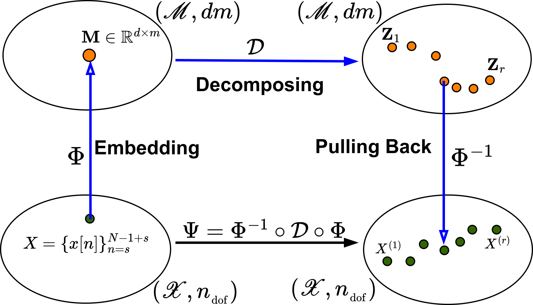
Figure 5: Pulling back theorem for deterministic time sequence

5.2.2 Random Time Sequence

For practical problems, the time sequence involved is usually random due to the noise in the process of capturing discrete time data with sensor. In order to filter the noise, it is necessary to introduce a denoising module which can be denoted by $\mathcal{F}$. Figure 6 illustrates this scenario intuitively.

We remark that the matrix components $\bm{Z}_{1},\cdots,\bm{Z}_{r}$ obtained by the decomposing module are perturbed by noise. After the denoising operation, we have

$$\sum^{\hat{r}}_{k=1}\hat{\bm{Z}}_{k}=\mathcal{F}\left(\sum^{r}_{i=1}\bm{Z}_{i}\right)$$ (40)

where $\hat{r}\leq r$ since some of the components may be removed and some the components may be modified. If the noise does not exist, then we have $r=\hat{r}$ and $\hat{\bm{Z}}_{k}=\bm{Z}_{k}$ or equivalently $\mathcal{F}=\mathbb{1}$ is the identity operator. Generally, we can obtain

$$\sum^{\hat{r}}_{k=1}\hat{X}^{(k)}=\Psi(X)=(\Phi^{-1}\circ\mathcal{F}\circ\mathcal{D}\circ\Phi)(X)$$ (41)

where $\hat{X}^{(k)}\in\mathscr{X}$ is the $k$-th estimated component of time sequence from the perturbed time sequence $X$ with the equivalent mode decomposition operator

$$\Psi=\Phi^{-1}\circ\mathcal{F}\circ\mathcal{D}\circ\Phi,\quad\mathrm{with~denoising}$$ (42)

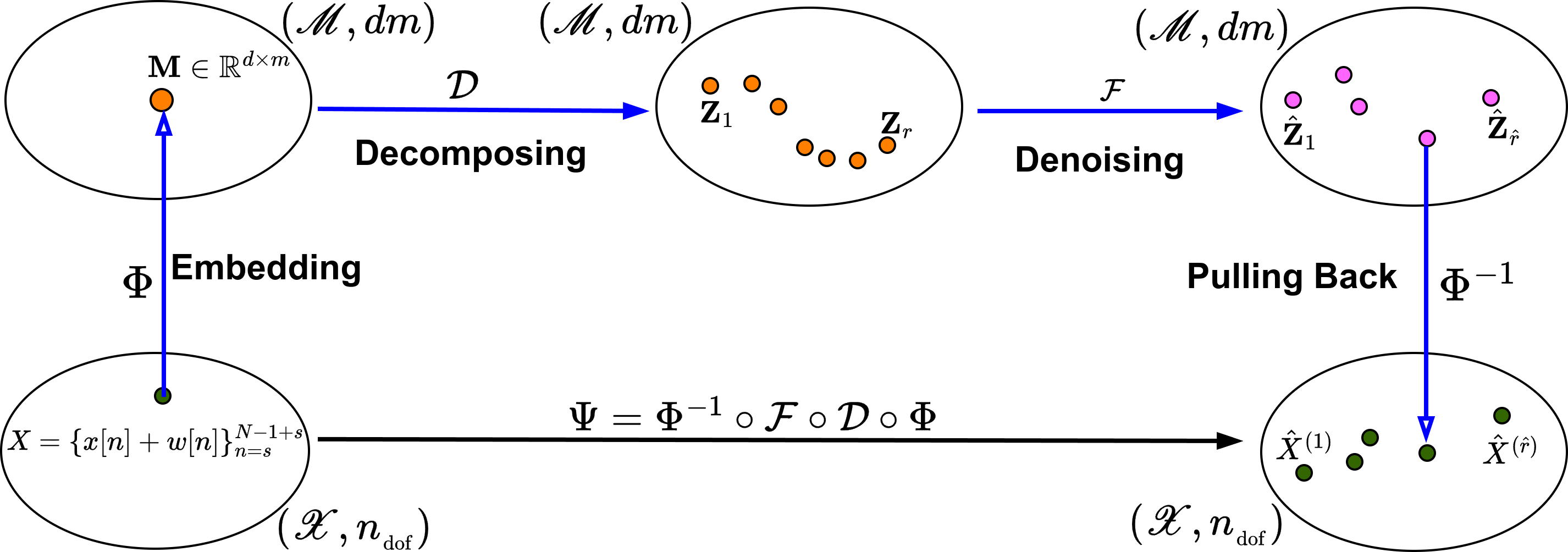
Figure 6: Pulling back theorem for random time sequence

It should be noted that the noise has important impact on the rebuilding process of $x^{(k)}[n]$ with the container (30). In the sense of rebuilding the $x^{(k)}[n]$ with $Q_{k}(n,\tau,s)$, the essence of (31) is just estimating the sequence $X^{(k)}=\left\{x^{(k)}[n]\right\}^{N-1+s}_{n=s}$ with simple arithmetic averaging.

Table 5: Relation of data set size $\left|Q_{k}(n,\tau,s)\right|$ and time delay $\tau$ for the given $(N,d,s,n)$

$N$	$d$	$s$	$n$	$\tau$	$\left|Q_{k}(n,\tau,s)\right|$	Remark
2000	100	1	213	1	100	$\tau\leq{\tau}_{\mathrm{max}}$
2000	100	1	213	2	100	$\tau\leq{\tau}_{\mathrm{max}}$
2000	100	1	213	3	71	$\tau\leq{\tau}_{\mathrm{max}}$
2000	100	1	213	4	54	$\tau\leq{\tau}_{\mathrm{max}}$
2000	100	1	213	5	43	$\tau\leq{\tau}_{\mathrm{max}}$
2000	100	1	213	6	36	$\tau\leq{\tau}_{\mathrm{max}}$
2000	100	1	213	7	31	$\tau\leq{\tau}_{\mathrm{max}}$
2000	100	1	213	8	27	$\tau\leq{\tau}_{\mathrm{max}}$
2000	100	1	213	9	24	$\tau\leq{\tau}_{\mathrm{max}}$
2000	100	1	213	10	22	$\tau\leq{\tau}_{\mathrm{max}}$
2000	100	1	213	11	20	$\tau\leq{\tau}_{\mathrm{max}}$
2000	100	1	213	12	18	$\tau\leq{\tau}_{\mathrm{max}}$
2000	100	1	213	13	17	$\tau\leq{\tau}_{\mathrm{max}}$
2000	100	1	213	14	16	$\tau\leq{\tau}_{\mathrm{max}}$
2000	100	1	213	15	15	$\tau\leq{\tau}_{\mathrm{max}}$
2000	100	1	213	16	14	$\tau\leq{\tau}_{\mathrm{max}}$
2000	100	1	213	17	13	$\tau\leq{\tau}_{\mathrm{max}}$
2000	100	1	213	18	12	$\tau\leq{\tau}_{\mathrm{max}}$
2000	100	1	213	19	7	$\tau\leq{\tau}_{\mathrm{max}}$
2000	100	1	213	20	1	$\tau>{\tau}_{\mathrm{max}}$

Table 5 illustrates the data set size $\left|Q_{k}(n,\tau,s)\right|$ for $(N,d,s,n)=(2000,100,1,213)$ and $\tau\in\left\{1,2,\cdots,20\right\}$. It is obvious that different time delay $\tau$ leads to different size $\left|Q_{k}(n,\tau,s)\right|$. Obviously, the value of $x[n]$ calculated by averaging depends on the elements of the data set $Q_{k}(n,\tau,s)$ and the size $\left|Q_{k}(n,\tau,s)\right|$. In order to estimate the value of $x[n]$, it is necessary to replace the arithmetic average estimator with a better estimator, say median filter or other proper estimator.

As the generalization of the pulling back theorem under the noisy free condition, we now give the revised version the pulling back theorem as follows:

Theorem  5.

For the type $s\in\left\{0,1\right\}$, embedding dimension $d\in\mathbb{N}$ and time sequence $X=\left\{x[n]\right\}^{N-1+s}_{n=s}$ of length $N$ perturbed by noise, we can pull back the $k$-th CTM $\bm{Z}_{k}=(Z^{i}_{j}(k))$ in the immersion space $\mathbb{R}^{{d}\times{m}}$ such that $\displaystyle\mathcal{D}(\bm{M})=\sum^{r}_{k=1}\bm{Z}_{k}$ to the $k$-th CTS ${x}_{\mathrm{cts}}^{(k)}[n]$ by

$${x}_{\mathrm{cts}}^{(k)}[n]=\textsc{MeanSolver}(Q_{k}(n,\tau,s),\left|Q_{k}(n,\tau,s)\right|)$$ (43)

where MeanSolver is the algorithm for sequence estimation by averaging the data set $Q_{k}(n,\tau,s)$.

Particularly, if the noisy does not exist, the filtering operator must be the identity operator and Theorem 5 degrades to Theorem 2 since $\mathcal{F}$ degrades to the identity operator $\mathbb{1}$ and the MeanSolver algorithm for state estimation can be implemented with arithmetic average algorithm AriAveSolver or median algorithm MedianSolver.

5.3 Impact of Time Delay

The time sequence $X=\left\{x[n]:s\leq n\leq N-1+s\right\}$ is usually obtained by sampling the continuous signal $x(t)$ with the sampling frequency $f$. Formally, we have

$$x[n]=x(t_{0}+n/f),\quad n\in\mathbb{Z}^{+},t\in[t_{0},{t}_{\mathrm{end}}]$$ (44)

for the initial time $t_{0}\in\mathbb{R}$ and final time ${t}_{\mathrm{end}}$. We have the following observation for configuring the time delay $\tau\in\mathbb{N}$:

• If the sampling frequency $f$ is high, then $N=\left\lfloor{({t}_{\mathrm{end}}-t_{0})f}\right\rfloor$ will be large. The smallest $\tau=1$ means a large integer $m=N-(d-1)\tau$ for the given embedding dimension $d$ when $N$ is large, which implies the matrix $\bm{M}$ of $d$-by-$m$ is a big matrix. For the matrix decomposition involved in the mode decomposition will lead to high computational complexity. In the sense of reducing the computational complexity of mode decomposition, we should set $\tau>1$ and a big $\tau$ may be better.

• For the fixed length $N$, embedding dimension $d$ and time delay $\tau$, we have

  $$\left|Q_{k}(n,\tau,s)\right|={q}_{\mathrm{max}}-{q}_{\mathrm{min}}+1$$ (45)

  and for the fixed $n$ and $s$, $\left|Q_{k}(n,\tau,s)\right|$ is decreasing when $\tau$ is increasing according to (29). In other words, a big $\tau$ means a small date set $Q_{k}(n,\tau,s)$, which lowers the performance of the estimation algorithm MeanSolver.

• For the time sequence perturbed by noise, it is wise to set a lower bound for the number of the columns for the trajectory matrix $\bm{M}\in\mathbb{R}^{{d}\times{m}}$, i.e.,

  $$m\geq d\geq 2{n}_{\mathrm{dof}}+1,$$ (46)

  which implies that

  $$\tau\leq\left\lfloor{\frac{N-d}{d-1}}\right\rfloor\leq\left\lfloor{\frac{N-(2{n}_{\mathrm{dof}}+1)}{d-1}}\right\rfloor$$ (47)

  Usually, the intrinsic dimension ${n}_{\mathrm{dof}}$ is not known and we can set the upper bound as

  $${\tau}_{\mathrm{max}}=\left\lfloor{\frac{N-d}{d-1}}\right\rfloor.$$ (48)

  As shown in Table 5, for the $(N,d)=(2000,100)$, we have ${\tau}_{\mathrm{max}}=\left\lfloor{1900/99}\right\rfloor=19$ and $\left|Q_{k}(213,19,1)\right|=7$ candidates can be for estimating the value of $x[213]$. Moreover, as shown in Table 4, we have ${m}_{\mathrm{min}}=119$. Otherwise, if we take $\tau=20$, then $m=20<d=100$ and only one candidate can be used for estimating $x[213]$, which should be avoided in statistical estimation.

In summary, we should balance the computational cost and the precision of the mode decomposition when configuring the time delay $\tau$ such that $1\leq\tau\leq{\tau}_{\mathrm{max}}$.

5.4 Application in Singular Spectrum Analysis

There are two significant issues that should be noted: firstly, the (27) is widely used for the trajectory matrix in singular spectrum analysis (SSA); secondly, the SSA with the DAP for converting trajectory matrix to time sequence is originally proposed by Vautard in 1992 [17]. Thus we can deduce that the SGMD and SSA share the common steps of embedding for up conversion and the DAP for down conversion. For the time delay $\tau=1$, the SGMD and SSA have the same trajectory matrix $\bm{M}=\Phi(X)$ if the $d$ and $m$ are the same. With the help of the pulling back theorem, the embedding of SSA can be replaced with the embedding mapping $\Phi$ used in the SGMD by allowing $\tau\geq 1$.

6 Conclusions

The original SGMD is limited to the two cases without doubts in the past five years:

• time delay $\tau=1$ in the inversion of embedding step, which is due to the dependence on the diagonal averaging principle;

• the embedding just holds for the type-1 time sequence denoted by $X=\left\langle x[1],x[2],\cdots,x[N]\right\rangle$ for the Fortran/MATLAB/Octave/… programming languages and fails for the type-0 time sequence denoted by $X=\left\langle x[0],x[1],\cdots,x[N-1]\right\rangle$ for the C/C++/Java/Python/Rust/… programming languages.

Our main conclusions include the following significant aspects:

• The pulling back theorem for inverting the embedding step in SGMD is proposed for deterministic time sequences with the theory of Diophantine equation in number theory for the general case of time delay $\tau\in\mathbb{N}$ and time sequence $X=\left\{x[n]\right\}^{N-1+s}_{n=s}$ for $s\in\left\{0,1\right\}$.

• In order to deal with random time sequences, the pulling back theorem is generalized by introducing a denoising step after decomposing the trajectory matrix and using a mean estimation algorithm for pulling back the CTM to the corresponding CTS.

• The discussion of how to configure the time delay $\tau$ in embedding step shows that small $\tau$ means better mean estimation but large computational complexity in matrix decomposition, thus a proper value $\tau$ is needed for balancing the efficiency and accuracy.

In the future work, we will propose novel version of the algorithms for SGMD with lower computational complexity and less constraints for the time delay, and exploring the relation of SSA and SGMD with our pulling back theorem.

Acknowledgments

This work was supported in part by the National Natural Science Foundation of China under grant numbers 62167003 and 62373042, in part by the Hainan Provincial Natural Science Foundation of China under grant numbers 720RC616 and 623RC480, in part by the Research Project on Education and Teaching Reform in Higher Education System of Hainan Province under grant number Hnjg2023ZD-26, in part by the Specific Research Fund of the Innovation Platform for Academicians of Hainan Province, in part by the Hainan Province Key R & D Program Project under grant number ZDYF2021GXJS010, in part by the Guangdong Basic and Applied Basic Research Foundation under grant number 2023A1515010275, and in part by the Foundation of National Key Laboratory of Human Factors Engineering under grant number HFNKL2023WW11.

Data Availability

Not applicable

Code Availability

Not applicable

Declaration of interests

The authors declare that they have no known competing financial interests or personal relationships that could have appeared to influence the work reported in this paper.

Appendix A Diophantine Equation $\tau x+y=n+s\tau$

For the Diophantine equation $ax+by=n$, we have the following important properties [20, 21]:

Theorem  6.

For $a,b\in\mathbb{N}=\left\{1,2,3,\cdots\right\}$ and $n\in\mathbb{Z}=\left\{0,\pm 1,\pm 2,\cdots\right\}$, the equation $ax+by=n$ has solution $(x,y)\in\mathbb{Z}^{2}$ if and only if the greatest common divisor of $a$ and $b$ is a factor of $n$, i.e., $\operatorname{GCD}(a,b)\mid n$.

Theorem  7.

Suppose that $a,b\in\mathbb{N}$ such that $\operatorname{GCD}(a,b)=1$. For any $n\in\mathbb{Z}$ such that $n>ab-a-b$, there must exist $x,y\in\mathbb{Z}^{+}=\left\{0,1,2,\cdots\right\}$ such that $n=ax+by$.

If we take the following assignment

$$\left\{\begin{aligned} a&\leftarrow\tau\\ b&\leftarrow 1\\ n&\leftarrow n+s\tau\end{aligned}\right.$$ (49)

for $s\in\left\{0,1\right\}$ and $\tau\in\mathbb{N}$, then the solution of the Diophantine equation $\tau x+y=n+s\tau$ have non-negative solution $(x,y)\in(\mathbb{Z}^{+})^{2}$ for any $n\in\mathbb{Z}^{+}$.

References

- [1] Haiyang Pan, Yu Yang, Xin Li, Jinde Zheng, and Junsheng Cheng. Symplectic geometry mode decomposition and its application to rotating machinery compound fault diagnosis. Mechanical Systems and Signal Processing, 114(1):189–211, 2019. https://doi.org/10.1016/j.ymssp.2018.05.019.
- [2] Hongbo Xie, Zhizhong Wang, and Hai Huang. Identification determinism in time series based on symplectic geometry spectra. Physics Letters A, 342(1-2):156–161, 2005. https://doi.org/10.1016/j.physleta.2005.05.035.
- [3] Hong-Bo Xie, Tianruo Guo, Bellie Sivakumar, Alan Wee-Chung Liew, and Socrates Dokos. Symplectic geometry spectrum analysis of nonlinear time series. Proceedings of the Royal Society A: Mathematical, Physical and Engineering Sciences, 470(2170):20140409, 2014. http://dx.doi.org/10.1098/rspa.2014.0409.
- [4] Floris Takens. Detecting strange attractors in turbulence. In Dynamical Systems and Turbulence, volume 898 of Lecture Notes in Mathematics, pages 366–381, Berlin, 1981. Springer-Verlag.
- [5] A. Salam, A. El Farouk, and E. Al-Aidarous. Symplectic Householder transformations for a QR-like decomposition, a geometric and algebraic approaches. Journal of Computational and Applied Mathematics, 214(2):533–548, 2008. https://doi.org/10.1016/j.cam.2007.03.015.
- [6] Jianchun Guo, Zetian Si, Yi Liu, Jiahao Li, Yanting Li, and Jiawei Xiang. Dynamic time warping using graph similarity guided symplectic geometry mode decomposition to detect bearing faults. Reliability Engineering & System Safety, 224:108533, 2022.
- [7] Hang Jin, jianhui Lin, Xieqi Chen, and Cai Yi. Modal parameters identification method based on symplectic geometry model decomposition. Shock and Vibration, 2019:5018732, 2019. https://doi.org/10.1155/2019/5018732.
- [8] Guangyao Zhang, Yi Wang, Xiaomeng Li, Baoping Tang, and Yi Qin. Enhanced symplectic geometry mode decomposition and its application to rotating machinery fault diagnosis under variable speed conditions. Mechanical Systems and Signal Processing, 170:108841, 2022. https://doi.org/10.1016/j.ymssp.2022.108841.
- [9] Jianchun Guo, Zetian Si, Yi Liu, Jiahao Li, Yanting Li, and Jiawei Xiang. Dynamic time warping using graph similarity guided symplectic geometry mode decomposition to detect bearing faults. Reliability Engineering & System Safety, 224:108533, 2022.
- [10] Jianchun Guo, Zetian Si, and Jiawei Xiang. Cycle kurtosis entropy guided symplectic geometry mode decomposition for detecting faults in rotating machinery. ISA Transactions, 138:546–561, 2023.
- [11] Yijie Chen, Zhenwei Guo, and Dawei Gao. Marine controlled-source electromagnetic data denoising method using symplectic geometry mode decomposition. Journal of Marine Science and Engineering, 11(8):1578, 2023. https://www.mdpi.com/2077-1312/11/8/1578.
- [12] Yanfei Liu, Junsheng Cheng, Yu Yang, Jinde Zheng, Haiyang Pan, Xingkai Yang, Guangfu Bin, and Yiping Shen. Symplectic sparsest mode decomposition and its application in rolling bearing fault diagnosis. IEEE Sensors Journal, 24(8):12756–12769, 2024. https://doi.org/10.1109/JSEN.2024.3370959.
- [13] Jingtang Hao, Long Ma, Xutao Yin, Xinyi Zhao, and Zhigang Su. Improved symplectic geometry mode decomposition based correlation method in white light scanning interferometry. Optics and Lasers in Engineering, 182:108482, 2024. https://doi.org/10.1016/j.optlaseng.2024.108482.
- [14] Pengming Zhan, Xianrong Qin, Qing Zhang, and Yuantao Sun. Output-only modal identification based on auto-regressive spectrum-guided symplectic geometry mode decomposition. Journal of Vibration Engineering & Technologies, 12(1):139–161, 2024. https://doi.org/10.1007/s42417-022-00832-1.
- [15] Ge Xin, Yifei Chen, Lingfeng Li, Chuanhai Chen, Zhifeng Liu, and Jérôme Antoni. Complex symplectic geometry mode decomposition and a novel time–frequency fault feature extraction method. IEEE Transactions on Instrumentation and Measurement, 74(1):1–10, 2025.
- [16] James C. Robinson. Dimensions, Embeddings, and Attractors, volume 186 of Cambridge Tracts in Mathematics. Cambridge University Press, London, 2010. https://doi.org/10.1017/CBO9780511933912, pages: 145–159.
- [17] Robert Vautard, Pascal Yiou, and Michael Ghil. Singular-spectrum analysis: A toolkit for short, noisy chaotic signals. Physica D: Nonlinear Phenomena, 58(1):95–126, 1992.
- [18] Jaime Zabalza, Jinchang Ren, Zheng Wang, Stephen Marshall, and Jun Wang. Singular spectrum analysis for effective feature extraction in hyperspectral imaging. IEEE Geoscience and Remote Sensing Letters, 11(11):1886–1890, 2014.
- [19] M. C. R. Leles, J. P. H. Sansão, L. A. Mozelli, and H. N. Guimarães. Improving reconstruction of time-series based in Singular Spectrum Analysis: A segmentation approach. Digital Signal Processing, 77(6):63–76, 2018. Digital Signal Processing & SoftwareX - Joint Special Issue on Reproducible Research in Signal Processing.
- [20] Loo Keng Hua. Introduction to Number Theory. Springer-Verlag, New York, 1982. the Chinese version was published by the Science Press in 1957.
- [21] Henri Cohen. Number Theory, Volume I: Tools and Diophantine Equations, volume 239 of Graduate Texts in Mathematics. Springer, New York, 2007.