On a Cahn–Hilliard equation for the growth and division of chemically active droplets modeling protocells

Abstract

The Cahn–Hilliard model with reaction terms can lead to situations in which no coarsening is taking place and, in contrast, growth and division of droplets occur which all do not grow larger than a certain size. This phenomenon has been suggested as a model for protocells, and a model based on the modified Cahn–Hilliard equation has been formulated. We introduce this equation and show the existence and uniqueness of solutions. Then formally matched asymptotic expansions are used to identify a sharp interface limit using a scaling of the reaction term which becomes singular when the interfacial thickness tends to zero. We compute planar solutions and study their stability under non-planar perturbations. Numerical computations for the suggested model are used to validate the sharp interface asymptotics. In addition, the numerical simulations show that the reaction terms lead to diverse phenomena such as growth and division of droplets in the obtained solutions, as well as the formation of shell-like structures.

Keywords: Cahn–Hilliard equation, chemical reactions, pattern formation, active droplets, protocells

AMS (MOS) Subject Classification: 35B25, 35K55, 35K61, 35R35, 35Q92.

1 Introduction

It has been proposed recently that chemical reactions in phase separating systems can lead to a suppression of Ostwald ripening and to the growth and division of droplets [32, 31, 6]. These systems are away from thermodynamic equilibrium with an external supply of energy enhancing chemical reactions. In [31] it was even demonstrated that droplets in the presence of chemical reactions can grow and spontaneously split. Then a further growth of divided droplets, using up the fuel from chemical reactions, is possible, leading eventually to further splitting. The model studied in [32, 31, 6] involves a Cahn–Hilliard model with chemical reactions, and in general, does not fulfill a free energy inequality. This is due to the fact that energy is supplied, and such systems are called active systems. In [31] the authors argue that such active systems can play an important role in the transition between nonliving and living systems. Initially, featureless aggregates of abiotic matter evolve and form protocells which can be the basis for systems that gain the structure and functions necessary to fulfill the criteria of life.

It was also shown in subsequent studies that synthetic analogues of such chemically active systems can be developed, see [16]. In such system not only Ostwald ripening is suppressed but also stable liquid shells can form, see [6, 8]. Here, a shell of one phase forms with an inside and an outside of a second phase. In fact, it was observed experimentally that spherical, active droplets can undergo a morphological transition into a spherical shell. In [8] it was shown that the mechanism is related to gradients of the droplet material, and the authors also identify how much chemical energy is necessary to sustain the spherical drop. The non-conservative Cahn–Hilliard system the authors of [31] introduced is

$$\partial_{t}{{\varphi}} =\mathop{\rm div}\nolimits(m({{\varphi}})\nabla\mu)+S_{\varepsilon}({{\varphi}}),$$

$$\mu =\beta(-\varepsilon\Delta{{\varphi}}+\tfrac{1}{\varepsilon}\psi^{\prime}({{\varphi}})),$$

where in this paper we take ${{\varphi}}$ to be the normalized concentration difference between the droplet material and the background material, which is scaled such that the two phases are at $\pm 1$. Besides, $\beta$ and $\varepsilon$ are constants, and $m$ and $S_{\varepsilon}$ are phase-dependent functions that will be introduced later. The variable $\mu$ is the chemical potential given as the first variation of a Ginzburg–Landau free energy given by

$${\cal E}({{\varphi}})=\beta\Big{(}\frac{\varepsilon}{2}\int_{\Omega}|\nabla{{\varphi}}|^{2}+\frac{1}{\varepsilon}\int_{\Omega}\psi({{\varphi}})\Big{)},$$ (1.2)

where $\psi$ represents a suitable double-well free energy density. Compared to the classical Cahn–Hilliard model the main new term is the reaction term $S_{\varepsilon}({{\varphi}})$ which in [31] was taken to be affine linear outside of the interfacial region that separates the two phases given by the droplet regions and the background region. Within the interfacial region an interpolation between these two affine linear functions is chosen. In the droplet phase $\{{{\varphi}}=1\}$, $S_{\varepsilon}(1)$ will be negative, which reflects the fact that the droplet material degrades chemically. In the background phase $\{{{\varphi}}=-1\}$, $S_{\varepsilon}(-1)$ will be positive, which takes into account that the material making up the droplet phase is produced in the background phase by chemical reactions involving a fuel which powers its production, see [31] for details.

In the case without chemical reactions, i.e., $S_{\varepsilon}=0$, the Cahn–Hilliard model was first formulated in [11] using the free energy (1.2) introduced in [12]. Since its introduction the Cahn–Hilliard equation has been the subject of many studies and has found many applications. We refer to [27, 26, 4] for detailed overviews. In particular, it can be shown that the Cahn–Hilliard model is the $H^{-1}$ gradient flow of the energy (1.2), see e.g., [19, 4]. Furthermore, it was also shown, first formally by Pego [28] and later rigorously by Alikakos, Bates and Chen [3], that the Cahn–Hilliard model converges to the Mullins–Sekerka sharp interface model as the interfacial thickness converges to zero. It was also demonstrated that the Cahn–Hilliard model can be used to describe the Ostwald ripening process, where small particles dissolve and larger ones grow, see [22]. There are numerous analytical results on the Cahn–Hilliard equation and we here only refer to the existence results in [18, 17] and to [2, 26] who, in particular, discuss the Cahn–Hilliard equation from a semi-group perspective and also study the physically relevant logarithmic potential.

Several models have been proposed in which a reaction type term $S_{\varepsilon}({{\varphi}})$ appears. The simplest one is the Cahn–Hilliard–Oono model in which $S_{\varepsilon}({{\varphi}})=-\omega({{\varphi}}-c^{*})$ with a positive constant $\omega$, and $c^{*}\in(-1,1)$ is given. This term accounts for nonlocal interactions in phase separation, see [26]. A proliferation term $S_{\varepsilon}({{\varphi}})=-\lambda{{\varphi}}(1-{{\varphi}})$ with a constant $\lambda>0$ has been introduced in [25]. For analytical results in this case we refer to [26]. A source term which depends on ${{\varphi}}$ but also depends on the spatial variable $x$ has been proposed in [9] for applications in binary image inpainting and was subsequently analysed in [10, 21], see also [30] for an application to image segmentation. In addition, in several tumor growth models, Cahn–Hilliard type models with source terms appear and are coupled to other equations, see, e.g., [14, 24, 20].

In this paper, we mathematically analyze the Cahn–Hilliard model introduced in [31]. We will first carefully introduce the model and then show a well-posedness result for the system. We use formally matched asymptotic expansions to relate the diffuse interface Cahn–Hilliard model to a new sharp interface model, which differs from the sharp interface model proposed in [31]. In particular, we will show that asymptotic expansions lead to a quasi-static diffusion problem also possibly involving source terms stemming from reactions at the interface. For the sharp interface model, we derive planar stationary solutions. Finally, we will use finite element computations for the Cahn–Hilliard model with reactions to numerically verify the matched asymptotics and to illustrate the stability and instability behavior of solutions. In particular, we will show several splitting scenarios as well as the formation of shell-like structures.

2 Mathematical models

2.1 The Cahn–Hilliard model

Let $\Omega$ be a bounded domain in $\mathbb{R}^{d}$, $d\in\{1,2,3\}$, with boundary $\partial\Omega$ containing two chemical species. We introduce a normalized difference ${{\varphi}}$ of the concentrations of two chemical components that is governed by the following Cahn–Hilliard equation with chemical reactions [31]:

$$\partial_{t}{{\varphi}} =\mathop{\rm div}\nolimits(m({{\varphi}})\nabla\mu)+S_{\varepsilon}({{\varphi}})\qquad Q:=(0,T)\times\Omega$$ in , (2.1a)

$$\mu =\beta(-\varepsilon\Delta{{\varphi}}+\tfrac{1}{\varepsilon}\psi^{\prime}({{\varphi}}))\qquad Q$$ in , (2.1b)

$$\partial_{{\bm{n}}}\mu =\partial_{{\bm{n}}}{{\varphi}}=0\qquad \Gamma:=(0,T)\times\partial\Omega$$ on , (2.1c)

$${{\varphi}}(0) ={{\varphi}}_{0}\qquad \Omega$$ in . (2.1d)

Here, $\mu$ is the associated chemical potential, $m{:{\mathbb{R}}\to{\mathbb{R}}_{>0}}$ is the concentration dependent mobility function, $\beta>0$ is a parameter related to a surface energy density, $\varepsilon>0$ is a small length scale proportional to the thickness of the diffuse interface function, $\psi{:{\mathbb{R}}\to{\mathbb{R}}_{\geq 0}}$ is a double well potential, $\partial_{{\bm{n}}}$ is the derivative in the direction of the unit outer normal ${\bm{n}}$ to $\partial\Omega$ and ${{\varphi}}_{0}$ serves as initial data for ${{\varphi}}$. We consider the above equations on the space-time cylinder ${Q}$ with a fixed but arbitrary time $T>0$.

The source term $S_{\varepsilon}:{\mathbb{R}}\to{\mathbb{R}}$ is given as

$$S_{\varepsilon}(r)=S_{1}(r)+\tfrac{1}{\varepsilon}S_{2}(r){,\quad r\in{\mathbb{R}}}.$$ (2.2)

Here, the term $S_{2}$ will later lead to a fast reaction in the interfacial region. On choosing $r_{c}\in(0,1]$, we set for constants $S_{+}$, $S_{-}$, $K_{+}$, $K_{-}$, and $L$

$$S_{1}(r)=\begin{cases}{S_{+}}&\quad\text{if $r\geq{r_{c}}$,}\\ {S_{-}}+G_{1}(r)({S_{+}}-{S_{-}})&\quad\text{if $r\in(-{r_{c}},{r_{c}})$,}\\ {S_{-}}&\quad\text{if $r\leq-{r_{c}}$,}\end{cases}$$ (2.3)

and

$$S_{2}(r)=\begin{cases}-{K_{+}}(r-1)&\quad\text{if $r\geq{r_{c}}$,}\\ \widehat{S}_{2}(r)&\quad\text{if $r\in(-{r_{c}},{r_{c}})$,}\\ -{K_{-}}(r+1)&\quad\text{if $r\leq-{r_{c}}$,}\end{cases}$$ (2.4)

where we define for $r\in(-{r_{c}},{r_{c}})$

$$\widehat{S}_{2}(r)=-{{K_{-}}}G_{2}(r)-{{K_{+}}}G_{3}(r)+LG_{4}(r){-K_{+}(r_{c}-1)G_{1}(r)-K_{-}(1-r_{c})(1-G_{1}(r))}.$$

Here, $G_{1},G_{2},G_{3},G_{4}:[-1,1]\to{\mathbb{R}}$ are suitable differentiable interpolation functions, to be introduced below, satisfying

$$G_{1}({r_{c}})=1,\quad G_{1}(-{r_{c}})=0,\quad G_{2}(\pm{r_{c}})=G_{3}(\pm{r_{c}})=G_{4}(\pm{r_{c}})=0,$$ (2.5)

$$G_{1}^{\prime}(\pm{r_{c}})=G_{4}^{\prime}(\pm{r_{c}})=0,\quad G_{2}^{\prime}({r_{c}})=G_{3}^{\prime}(-{r_{c}})=0,\quad G_{2}^{\prime}(-{r_{c}})=G_{3}^{\prime}({r_{c}})=1,$$ (2.6)

so that the source term $S_{\varepsilon}$ is differentiable on ${\mathbb{R}}$. We often use $r_{c}=1$ which considerably simplifies the expression for $\widehat{S}_{2}$ and the matched asymptotic expansions which we use later to derive a sharp interface limit. However, other choices can also be considered, such as $r_{c}=\frac{1}{2}$ as in [31].

The system (2.1) is related to the following free energy

$${\cal E}({{\varphi}})=\beta\Big{(}\frac{\varepsilon}{2}\int_{\Omega}|\nabla{{\varphi}}|^{2}+\frac{1}{\varepsilon}\int_{\Omega}\psi({{\varphi}})\Big{)}.$$

In what follows we assume that $\psi$ is even, that is $\psi(r)=\psi(-r)$ for $r\in{\mathbb{R}}$, and satisfies $\psi(\pm 1)=0$ and $\psi^{\prime\prime}(\pm 1)\neq 0$. Typically, we will choose the quartic potential

$$\psi(r)=\tfrac{1}{4}(1-r^{2})^{2},\quad r\in{\mathbb{R}}.$$ (2.7)

2.2 Possible choice of the interpolation functions

As mentioned above, in the theoretical analysis to follow, we consider any interpolation functions $G_{1}$, $G_{2}$, $G_{3}$ and $G_{4}$ such that (2.5)–(2.6) are fulfilled. Here, we present a possible choice related to the double well potential $\psi$. We set, for every $r\in[-1,1]$,

$$G_{1}(r){=\widehat{G}_{1}(\tfrac{r}{r_{c}}),\quad\widehat{G}_{1}(r)} =\tfrac{3}{4}(r+1)^{2}-\tfrac{1}{4}(r+1)^{3},$$ (2.8)

$$G_{2}(r){=r_{c}\widehat{G}_{2}(\tfrac{r}{r_{c}}),\quad\widehat{G}_{2}(r)} =-{\tfrac{1}{2}}\tfrac{1}{\sqrt{\psi^{\prime\prime}(-1)}}(r-1)\sqrt{2\psi(r)},\quad G_{3}(r)=-G_{2}(-r),$$ (2.9)

and observe that

$$\widehat{G}_{1}(1)=1,\quad\widehat{G}_{1}(-1)=G_{1}^{\prime}(\pm 1)=0,\quad\widehat{G}_{2}(\pm 1)=0,\quad\widehat{G}_{2}^{\prime}(1)=0,\quad\widehat{G}_{2}^{\prime}(-1)=1.$$

We just provide the details for verifying $\widehat{G}_{2}^{\prime}(-1)={1}$ as the others are straightforward. For convenience, let us set $c^{*}:=-{\frac{1}{2}}\frac{1}{\sqrt{\psi^{\prime\prime}(-1)}}$ so that

$$\widehat{G}_{2}^{\prime}(-1)=\frac{d}{dr}\widehat{G}_{2}(r)\Big{|}_{r=-1}=c^{*}\Big{(}\sqrt{2\psi(r)}+(r-1)\frac{d}{dr}\sqrt{2\psi(r)}\Big{)}\Big{|}_{r=-1}=-2{c^{*}}\frac{d}{dr}\sqrt{2\psi(r)}\Big{|}_{r=-1}.$$

For the argument in the latter expression, using Taylor’s expansion, it holds that

$$\psi(r)=\underbrace{\psi(-1)}_{=0}+\underbrace{\psi^{\prime}(-1)(r+1)}_{=0}+\frac{1}{2}\psi^{\prime\prime}(-1)(r+1)^{2}+o\big{(}(r+1)^{2}\big{)},\quad r\in{\mathbb{R}},$$

whence we infer that

$$\frac{d}{dr}\sqrt{2\psi(r)}\Big{|}_{r=-1}=\lim_{r\searrow-1}\frac{\sqrt{\psi^{\prime\prime}(-1)}\,|r+1|}{r+1}=\sqrt{\psi^{\prime\prime}(-1)}.$$

Thus, using the definition of $\widehat{G}_{2}$ as stated above, we infer that $\widehat{G}_{2}^{\prime}(-1)=1$, as claimed. Note that due to the relation $\widehat{G}_{3}(r)=-\widehat{G}_{2}(-r)$ the condition $\widehat{G}_{3}^{\prime}(1)=1$ can be inferred in the same way. In particular, for the quartic potential (2.7), we have $\psi^{\prime\prime}(-1)=2$, and so

$$\widehat{G}_{2}(r)=-\tfrac{1}{4}(1-r^{2})(r-1),\quad\widehat{G}_{3}(r)=-\widehat{G}_{2}(-r)=-\tfrac{1}{4}(1-r^{2})(r+1)$$

which fulfill (2.5) and (2.6), respectively. In addition, we set

$$G_{4}(r){=\widehat{G}_{4}(\tfrac{r}{r_{c}}),\quad\widehat{G}_{4}(r)}=2\psi(r){,}\quad r\in\mathbb{R},$$ (2.10)

which clearly satisfies (2.5) and (2.6).

2.3 The sharp interface model

We now present the corresponding sharp interface system related to the Cahn–Hilliard model above. We will later use the method of formally matched asymptotic expansions, see, e.g., [4], to derive this free boundary problem. We denote by $\Omega^{\pm}=\Omega^{\pm}(t)$ the two regions occupied by the pure phases and by $\Sigma=\Sigma(t)$ the evolving interface separating the two phases. In addition, let $m_{\pm}:=m(\pm 1)$ be the mobilities in the two phases. The free boundary problem corresponding to (2.1) reads as follows:

$$-m_{+}\Delta\mu ={S_{+}}-\rho_{+}\mu\quad \Omega^{+}$$ in , (2.11a)

$$-m_{-}\Delta\mu ={S_{-}}-\rho_{-}\mu\quad \Omega^{-}$$ in , (2.11b)

$$\mu =\frac{\gamma\beta\kappa}{2}\qquad \Sigma$$ on , (2.11c)

$$[\mu]^{+}_{-} =0\qquad \Sigma$$ on , (2.11d)

$$-2{\cal V} =[m\nabla\mu]^{+}_{-}\cdot{{\bm{\nu}}}+S_{I}\qquad \Sigma$$ on , (2.11e)

$$\partial_{{\bm{n}}}\mu =0\qquad \partial\Omega$$ on , (2.11f)

where $\rho_{\pm}=\frac{K_{\pm}}{\beta\psi^{\prime\prime}(\pm 1)}$, $\gamma$ is a constant depending on the choice of the double well potential $\psi$ and $S_{I}$ is the interface reaction term which depends on the choice of the interpolation functions $G_{2}$, $G_{3}$ and $G_{4}$ (cf. (4.13)). In the case of the quartic potential and $r_{c}=1$, we will obtain

$$\rho_{\pm}=\frac{K_{\pm}}{2\beta},\quad\gamma=\frac{2\sqrt{2}}{3},\quad S_{I}=\frac{1}{\sqrt{2}}\Big{(}K_{+}-K_{-}+\frac{4}{3}L\Big{)}.$$

In the above, we also use $\kappa$ to denote the mean curvature of $\Sigma$ that is given as the sum of the principal curvatures of $\Sigma$, ${\bm{\nu}}$ is the unit normal to the interface, and ${\cal V}$ is the normal velocity of the interface in the direction of the normal ${\bm{\nu}}$. In addition, for $x\in\Sigma(t)$ and a function $u$, we define its jump across the interface at $(t,x)$ as

$$[u]^{+}_{-}(t,x):=\lim_{\begin{subarray}{c}y\to x\\ y\in\Omega^{+}(t)\end{subarray}}u(t,y)-\lim_{\begin{subarray}{c}y\to x\\ y\in\Omega^{-}(t)\end{subarray}}u(t,y)\,.$$

Further information about the notation used can be found in [4].

Notice that the above system is connected to the well-known Mullins–Sekerka free boundary problem [4], with the differences that here we have a constant source term $S_{I}$ on the right-hand side of (2.11e) as well as an affine linear term in the quasi-static diffusion equations (2.11a) and (2.11b).

2.4 Nondimensionalization for the sharp interface problem

We now perform a nondimensionalization argument in order to identify important dimensionless parameters. Choosing units $\widetilde{x}$, $\widetilde{t}$ and $\widetilde{\mu}$ for length, time and chemical potential we introduce the nondimensional variables

$$\widehat{x}=\frac{x}{\widetilde{x}},\quad\widehat{t}=\frac{t}{\widetilde{t}},\quad\widehat{\mu}=\frac{\mu}{\widetilde{\mu}}{,}$$

and now consider the rescaled variant of system (2.1) on the rescaled domains $\widehat{\Omega}^{+}$, $\widehat{\Omega}^{-}$, and the corresponding interface $\widehat{\Sigma}$. Denoting by $\widehat{\nabla}$ and $\widehat{\Delta}$ the gradient and Laplacian with respect to $\widehat{x}$, for the new nondimensional variables, we obtain from (2.11) the following system

$$-\widehat{\Delta}\widehat{\mu} =\frac{(\widetilde{x})^{2}}{m_{+}\widetilde{\mu}}{S_{+}}-\frac{(\widetilde{x})^{2}\rho_{+}}{m_{+}}\widehat{\mu}\quad \text{in $\widehat{\Omega}^{+}$},$$

$$-\widehat{\Delta}\widehat{\mu} =\frac{(\widetilde{x})^{2}}{m_{-}\widetilde{\mu}}{S_{-}}-\frac{(\widetilde{x})^{2}\rho_{-}}{m_{-}}\widehat{\mu}\quad \widehat{\Omega}^{-}$$ in ,

$$\widehat{\mu} =\frac{\gamma\beta\widehat{\kappa}}{2\widetilde{\mu}\widetilde{x}}\qquad \widehat{\Sigma}$$ on ,

$$[\widehat{\mu}]^{+}_{-} =0\qquad \widehat{\Sigma}$$ on ,

$$-2{\cal\widehat{V}} =\tfrac{\widetilde{t}\widetilde{\mu}}{(\widetilde{x})^{2}}[m\widehat{\nabla}\widehat{\mu}]^{+}_{-}\cdot{\widehat{{\bm{\nu}}}}+\tfrac{\widetilde{t}}{\widetilde{x}}S_{I}\qquad {\widehat{\Sigma}}$$ on ,

$$\partial_{{\bm{n}}}\widehat{\mu} =0\qquad {\partial\widehat{\Omega}}$$ on ,

with $\widehat{{\cal V}}$ being the normal velocity of the interface $\widehat{\Sigma}$ in the direction of the normal $\widehat{{\bm{\nu}}}$. To obtain simple nondimensional equations, and on assuming that $\rho_{-}>0$ and $S_{-}>0$, we set

$$\widetilde{x}=\sqrt{\frac{{m_{-}}}{\rho_{-}}},\quad\widetilde{\mu}=\frac{(\widetilde{x})^{2}S_{-}}{m_{-}}=\frac{S_{-}}{\rho_{-}},\quad\widetilde{t}=\frac{(\widetilde{x})^{2}}{\widetilde{\mu}m_{-}}=\frac{1}{S_{-}}.$$

We now define the nondimensional parameter

$$\beta^{*}=\frac{\beta}{\widetilde{x}}\frac{1}{\widetilde{\mu}}=\frac{\beta\rho_{-}^{\tfrac{3}{2}}}{m_{-}^{\frac{1}{2}}S_{-}}=\frac{c_{l}}{\widetilde{x}},$$

where we call

$$c_{l}=\beta\frac{\rho_{-}}{S_{-}}{,}$$ (2.13)

in analogy to solidification problems, the modified capillary length. In addition, we introduce the relative mobility $m^{*}$, the relative reaction coefficients $S^{*}$ and $\rho^{*}$, and the nondimensional interface reaction term $S_{I}^{*}$ as follows

$$m^{*}=\frac{m_{+}}{m_{-}},\quad S^{*}=\frac{S_{+}}{S_{-}},\quad\rho^{*}=\frac{\rho_{+}}{\rho_{-}},\quad S_{I}^{*}=\frac{\widetilde{t}}{\widetilde{x}}S_{I}=\frac{1}{S_{-}}\sqrt{\frac{\rho_{-}}{m_{-}}}S_{I}.$$

We then obtain, dropping the hat notation for convenience,

$$-m^{*}\Delta\mu =S^{*}-\rho^{*}\mu\quad \Omega^{+}$$ in ,

$$-\Delta\mu =1-\mu\quad \text{in $\Omega^{-}$},$$

$$\mu =\frac{\gamma\beta^{*}\kappa}{2}\qquad \Sigma$$ on ,

$$[\mu]^{+}_{-} =0\qquad \Sigma$$ on ,

$$-2{\cal V} =m^{*}\nabla\mu_{+}\cdot{{\bm{\nu}}}-\nabla\mu_{-}\cdot{{\bm{\nu}}}+S_{I}^{*}\qquad \Sigma$$ on ,

$$\partial_{{\bm{n}}}\mu =0\qquad \partial\Omega$$ on ,

and observe that the evolution critically depends on the nondimensional number $\beta^{*}$ which relates the influence of surface tension to a generalized supersaturation stemming from chemical reactions.

3 Well-posedness

In this section, we address the well-posedness of the system (2.1), aiming to cover a wide spectrum of scenarios. Specifically, we aim to accommodate various configurations without relying on the specific structure of the source term $S_{\varepsilon}$, as long as its growth is under control. Furthermore, in our analysis we can include rather general potentials, provided they are regular, nonsingular and exhibit polynomial growth. Let us first specify the notation we need for the well-posedness result.

3.1 Notation

Let $\Omega$ be a bounded domain in $\mathbb{R}^{d}$, $d\in\{2,3\}$, with boundary $\partial\Omega$. The Lebesgue measure of $\Omega$ is denoted by $|\Omega|$, while the Hausdorff measure of $\partial\Omega$ is denoted by $|\partial\Omega|$.

For any Banach space $X$, its norm is represented as $\|\cdot\|_{X}$, its dual space as $X^{*}$, and the duality pairing between $X^{*}$ and $X$ is denoted by $\langle\cdot,\cdot\rangle_{X}$. In the case where $X$ is a Hilbert space, the inner product is denoted by $(\cdot,\cdot)_{X}$.

For each $1\leq p\leq\infty$ and $k\geq 0$ the standard Lebesgue and Sobolev spaces defined on $\Omega$ are denoted as $L^{p}(\Omega)$ and $W^{k,p}(\Omega)$, with their respective norms $\|\cdot\|_{L^{p}(\Omega)}$ and $\|\cdot\|_{W^{k,p}(\Omega)}$. For simplicity we may often use $\|\cdot\|_{L^{p}}$ instead of $\|\cdot\|_{L^{p}(\Omega)}$, and employ similar shorthand notation for other norms. We adopt the convention $H^{k}(\Omega):=W^{k,2}(\Omega)$ for all $k\in\mathbb{N}$, and denote the mean value of a functional $h\in{(H^{1}(\Omega))^{*}}$ as

$$h_{\Omega}:=\frac{1}{|\Omega|}\langle h,1\rangle_{H^{1}}.$$

We now introduce a tool commonly employed in the investigation of problems associated with equations of Cahn–Hilliard type. Given $\phi\in{(H^{1}(\Omega))^{*}}$, we seek $u\in H^{1}(\Omega)$ such that

$$\int_{\Omega}\nabla u\cdot\nabla v=\langle\phi,v\rangle_{H^{1}},\quad v\in H^{1}(\Omega).$$ (3.1)

This corresponds to the standard weak formulation of the homogeneous Neumann problem for the Poisson equation $-\Delta u=\phi$ for $\phi\in L^{2}(\Omega)$. The solvability of (3.1) for $\phi\in{(H^{1}(\Omega))^{*}}$ relies on the condition that $\phi$ possesses a zero mean value, that is, $\phi_{\Omega}=0$. If this condition is satisfied, a unique solution with a zero mean value exists and the operator ${\cal N}:\text{dom}({\cal N})=\{\phi\in{(H^{1}(\Omega))^{*}}:\phi_{\Omega}=0\}\to\{u\in H^{1}(\Omega):u_{\Omega}=0\}$ defined by mapping $\phi$ to the unique solution $u$ to (3.1) with $u_{\Omega}=0$ is well-defined. This operator yields an isomorphism between the mentioned spaces. Additionally, the norm

$$\phi\mapsto\|\phi\|_{*}^{2}:=\|\nabla{\cal N}(\phi-{\phi_{\Omega}})\|^{2}_{L^{2}}+|\phi_{\Omega}|^{2},\quad\phi\in{(H^{1}(\Omega))^{*}},$$

is proven to define a Hilbert norm in ${(H^{1}(\Omega))^{*}}$ that is equivalent to the standard dual norm. From these definitions, it directly follows that

$$\int_{\Omega}\nabla{\cal N}\phi\cdot\nabla v=\langle\phi,v\rangle_{H^{1}}\quad \text{for every $\phi\in\text{dom}({\cal N})$ and $v\in H^{1}(\Omega)$},$$

$$\langle\phi,{\cal N}\zeta\rangle_{H^{1}}=\langle\zeta,{\cal N}\phi\rangle_{H^{1}}\quad \text{for every $\phi,\zeta\in\text{dom}({\cal N})$},$$

$$\langle\phi,{\cal N}\phi\rangle_{H^{1}}=\mathopen{\|}\nabla{\cal N}\phi\mathclose{\|}_{L^{2}}^{2}=\|\phi\|_{*}^{2}\quad \text{for every $\phi\in\text{dom}({\cal N})$}.$$

Moreover, it is established that

$$\int_{0}^{t}\langle\partial_{t}v(s),{\cal N}v(s)\rangle_{H^{1}}\,ds=\int_{0}^{t}\langle v(s),{\cal N}(\partial_{t}v(s))\rangle_{H^{1}}\,ds=\frac{1}{2}\|v(t)\|_{*}^{2}-\frac{1}{2}\|v(0)\|_{*}^{2}$$

for every $t\in[0,T]$ and $v\in H^{1}(0,T;{(H^{1}(\Omega))^{*}})$ such that $v_{\Omega}(t)=0$ for every $t\in[0,T]$.

3.2 Assumptions

For the well-posedness, we require the following assumptions.

1. The symbols $K_{\pm}$ and $S_{\pm}$ denote real valued constants, whereas $\beta$ and $\varepsilon$ denote positive constants.

2. The potential $\psi:{\mathbb{R}}\to[0,\infty)$ is twice differentiable and can be decomposed as $\psi=\psi_{1}+\psi_{2}$, with $\psi_{1}$ convex and $\psi_{2}$ a quadratic perturbation. Namely, we require that there exist a positive constant $C_{1}$ such that it holds

   $$|\psi_{2}(r)|\leq C_{1}(|r|^{2}+1){,}\quad r\in{\mathbb{R}},$$

   and in addition, we require

   $$\forall\eta>0\,\exists\,C_{\eta}:{\forall r\in{\mathbb{R}}}\quad|\psi^{\prime}(r)| \leq\eta\psi(r)+C_{\eta}.$$

3. We require the source $S_{\varepsilon}$ to be Lipschitz continuous. Consequently, there exists a positive constant $C_{S}$ such that

   $$|S_{\varepsilon}(r)|\leq C_{S}(|r|+1),\quad r\in{\mathbb{R}}.$$

4. The mobility function $m:{\mathbb{R}}\to{\mathbb{R}}$ is continuous and there exist positive constants $m_{*}$ and $M^{*}$ such that

   $$0<m_{*}\leq m(r)\leq M^{*},\quad r\in{\mathbb{R}}.$$

Let us notice that assumption (3.2) restricts the class of admissible double-well potentials, but still includes the quartic potential in (2.7). For this latter, referring to $\bm{({\mathrm{A2}})}$, we employ the splitting

$$\psi_{1}(r)=\tfrac{1}{4}r^{4},\quad\psi_{2}(r)=\tfrac{1}{4}(1-2r^{2}),\quad r\in{\mathbb{R}}.$$

Here is our main result.

Theorem 3.1.

Suppose that $\bm{({\mathrm{A1}})}$–$\bm{({\mathrm{A4}})}$ are fulfilled. Then, for every given ${{\varphi}}_{0}\in{H^{1}(\Omega)}$ there exists a weak solution $({{\varphi}},\mu)$ to (2.1) such that

$${{\varphi}} \in H^{1}(0,T;{(H^{1}(\Omega))^{*}})\cap L^{\infty}(0,T;H^{1}(\Omega))\cap L^{2}(0,T;H^{2}(\Omega)),$$

$$\mu \in L^{2}(0,T;H^{1}(\Omega)),$$

and satisfying

$$\mathopen{\langle}\partial_{t}{{\varphi}},v\mathclose{\rangle}_{{H^{1}}}+\int_{\Omega}m({{\varphi}})\nabla\mu\cdot\nabla v=\int_{\Omega}S_{\varepsilon}({{\varphi}})v,$$

$$\int_{\Omega}\mu v=\beta\varepsilon\int_{\Omega}\nabla{{\varphi}}\cdot\nabla v+\frac{\beta}{\varepsilon}\int_{\Omega}\psi^{\prime}({{\varphi}})v,$$

for every $v\in H^{1}(\Omega)$ and almost every $t\in(0,T)$, along with attainment of the initial condition $\varphi(0)=\varphi_{0}$ holding for almost every $x\in\Omega$.

Moreover, let $\{({{\varphi}}_{i},\mu_{i})\}_{i}$, $i=1,2$, denote two arbitrary solutions to (2.1) associated with initial data ${{\varphi}}_{0,i}\in H^{1}(\Omega)$, $i=1,2$ and to a constant mobility $m$. In addition, let us assume that there exists $p\in[1,7)$ such that $\psi_{1}^{\prime}$ satisfies the following pointwise growth condition

$$|\psi_{1}^{\prime}(r)-\psi_{1}^{\prime}(s)|\leq C(1+|r|^{p}+|s|^{p})|r-s|,\quad r,s\in{\mathbb{R}}.$$ (3.2)

Then, it holds that

$$\mathopen{\|}({{\varphi}}_{1}-{{\varphi}}_{2})-({{\varphi}}_{1}-{{\varphi}}_{2})_{\Omega}\mathclose{\|}_{L^{\infty}(0,T;{(H^{1}(\Omega))^{*}})\cap L^{2}(0,T;H^{1}(\Omega))}+\mathopen{\|}({{\varphi}}_{1})_{\Omega}-({{\varphi}}_{2})_{\Omega}\mathclose{\|}_{L^{\infty}(0,T)}$$

$$\quad\leq{C^{*}}\big{(}{\mathopen{\|}({{\varphi}}_{0,1}-{{\varphi}}_{0,2})-(({{\varphi}}_{0,1})_{\Omega}-({{\varphi}}_{0,2})_{\Omega})\mathclose{\|}_{*}}+|({{\varphi}}_{0,1})_{\Omega}-({{\varphi}}_{0,2})_{\Omega}|\big{)},$$

for a positive constant ${C}^{*}$ just depending on $\Omega$, $T$ and the nonlinearity $\psi$. Consequently, under these conditions the weak solution to (2.1) is unique.

Proof of Theorem 3.1.

We begin with the existence part of the theorem. In the subsequent discussion, we adopt a formal approach, leveraging standard procedures to derive estimates for the solution. While these computations are formal, they suggest that the same estimates can be rigorously applied to the $k$-dimensional system obtained via a Faedo–Galerkin scheme, constructed using the first $k$ eigenfunctions of the Laplace operator with homogeneous Neumann boundary conditions. These bounds can then be used to pass to the limit as $k\to\infty$, thereby constructing a solution to the problem that satisfies (2.1). A rigorous proof can be easily adapted within this approximation framework. Furthermore, in what follows, since we will need to make numerous estimates, we will agree to use $C$ to denote any nonnegative constant depending on the system’s data, which may change its value from line to line.

First estimate: Before starting with the proper estimates, let us introduce a new function related to the phase-dependent mobility function $m$. We set

$$M^{\prime}(z)=\int_{0}^{z}\frac{1}{m(s)}ds,\quad z\in{\mathbb{R}},$$

call $M$ a suitable antiderivative of it and notice that $M\in C^{2}({\mathbb{R}})$ and $M^{\prime\prime}(r)=\frac{1}{m(r)}$, $r\in{\mathbb{R}}$. Due to the bounds on $m$ in $\bm{({\mathrm{A4}})}$, we also have that there exist two positive constants $c_{1}$ and $c_{2}$ such that

$$c_{1}(1+|r|)\leq|M^{\prime}(r)|\leq c_{2}(1+|r|),\quad r\in{\mathbb{R}}.$$

We then test (2.1a) with $M^{\prime}({{\varphi}})$, (2.1b) with $-\Delta{{\varphi}}$ and add the resulting identities to obtain

$$\frac{1}{2}\frac{d}{dt}\mathopen{\|}M({{\varphi}})\mathclose{\|}^{2}_{L^{2}}+\beta\varepsilon\mathopen{\|}\Delta{{\varphi}}\mathclose{\|}^{2}_{L^{2}}+\frac{\beta}{\varepsilon}\int_{\Omega}\psi_{1}^{\prime\prime}({{\varphi}})|\nabla{{\varphi}}|^{2}=\int_{\Omega}S_{\varepsilon}({{\varphi}})M^{\prime}({{\varphi}})-\frac{\beta}{\varepsilon}\int_{\Omega}\psi_{2}^{\prime\prime}({{\varphi}})|\nabla{{\varphi}}|^{2},$$

where we notice that the third term on the left-hand side is nonnegative due to $\bm{({\mathrm{A2}})}$. Now, since $M^{\prime}$ is growing linearly, using $\bm{({\mathrm{A1}})}$–$\bm{({\mathrm{A4}})}$, we readily infer from Young’s inequality that the right-hand side is bounded from above by $C(\mathopen{\|}{{\varphi}}\mathclose{\|}^{2}_{L^{2}}+1)$. Using Grönwall’s inequality then produces

$$\mathopen{\|}M({{\varphi}})\mathclose{\|}_{L^{\infty}(0,T;L^{2}(\Omega))}+\mathopen{\|}\Delta{{\varphi}}\mathclose{\|}_{L^{2}(0,T;L^{2}(\Omega))}\leq C.$$

Besides, since $M^{\prime}$ is growing linearly, $M$ grows quadratically, so that from the above inequality we obtain, using also elliptic regularity theory, that

$$\mathopen{\|}{{\varphi}}\mathclose{\|}_{L^{\infty}(0,T;L^{2}(\Omega))\cap L^{2}(0,T;H^{2}(\Omega))}\leq C.$$

Second estimate: Next, recalling $\bm{({\mathrm{A2}})}$, upon testing (2.1b) with $\frac{1}{|\Omega|}$ yields

$$\mathopen{\|}\mu_{\Omega}\mathclose{\|}_{L^{2}(0,T)}\leq C,$$

where we also used the Sobolev embedding $H^{2}(\Omega){\hookrightarrow}L^{\infty}(\Omega)$.

Third estimate: We now perform the usual energy estimate in the context of the Cahn–Hilliard equation by testing (2.1a) with $\mu$, (2.1b) with $-\partial_{t}{{\varphi}}$ and adding the resulting identities to obtain

$$\frac{d}{dt}{\cal E}({{\varphi}})+\mathopen{\|}\nabla\mu\mathclose{\|}^{2}_{L^{2}}=\int_{\Omega}S_{\varepsilon}({{\varphi}})\mu=\int_{\Omega}S_{\varepsilon}({{\varphi}})(\mu-\mu_{\Omega})+\int_{\Omega}S_{\varepsilon}({{\varphi}})\mu_{\Omega}=I_{1}+I_{2}.$$

Now, employing the Young inequality and $\bm{({\mathrm{A3}})}$, we infer that

$$|I_{1}| \leq C(\mathopen{\|}{{\varphi}}\mathclose{\|}_{L^{2}}+1)\mathopen{\|}\nabla\mu\mathclose{\|}_{L^{2}}\leq\tfrac{1}{2}\mathopen{\|}\nabla\mu\mathclose{\|}^{2}_{L^{2}}+C{(}\mathopen{\|}{{\varphi}}\mathclose{\|}^{2}_{L^{2}}{+1)},$$

$$|I_{2}| \leq C(\mathopen{\|}{{\varphi}}\mathclose{\|}_{L^{2}}+1)|\mu_{\Omega}|\leq C{(}\mathopen{\|}{{\varphi}}\mathclose{\|}^{2}_{L^{2}}{+1)}+|\mu_{\Omega}|^{2}.$$

Thus, using the Poincaré–Wirtinger inequality and also the previous estimates readily entails that

$$\mathopen{\|}{{\varphi}}\mathclose{\|}_{L^{\infty}(0,T;H^{1}(\Omega))}+\mathopen{\|}\mu\mathclose{\|}_{L^{2}(0,T;H^{1}(\Omega))}\leq C.$$

Fourth estimate: Finally, it is standard to infer from the previous estimates and the weak formulation (2.1a) that

$$\mathopen{\|}\partial_{t}{{\varphi}}\mathclose{\|}_{L^{2}(0,T;{(H^{1}(\Omega))^{*}})}\leq C.$$

This concludes the existence part of the proof.

Moving to the uniqueness part, we consider two solutions $\{({{\varphi}}_{i},\mu_{i})\}_{i}$, $i=1,2$, associated to initial data ${{\varphi}}_{0,i}$, $i=1,2$ and recall that the mobility is assumed to be constant. Then, we introduce the notation

$${{\varphi}}={{\varphi}}_{1}-{{\varphi}}_{2},\quad\mu=\mu_{1}-\mu_{2},\quad{{\varphi}}_{0}={{\varphi}}_{0,1}-{{\varphi}}_{0,2},$$

and consider the system (2.1) written for the differences. Considering the difference of (2.1a), recalling the Lipschitz continuity of $S_{\varepsilon}$, and testing it with ${{\varphi}}_{\Omega}=({{\varphi}}_{1})_{\Omega}-({{\varphi}}_{2})_{\Omega}$ produces

$$\frac{d}{dt}\Big{(}\frac{1}{2}|{{\varphi}}_{\Omega}|^{2}\Big{)}\leq C|{{\varphi}}_{\Omega}|^{2}+C\mathopen{\|}{{\varphi}}\mathclose{\|}^{2}_{L^{2}}.$$ (3.3)

Then, we consider the difference of (2.1a) minus its mean value and test it with ${\cal N}({{\varphi}}-{{\varphi}}_{\Omega})$, the difference of (2.1b) and test it with $-({{\varphi}}-{{\varphi}}_{\Omega})$ and, upon adding the resulting equalities, we obtain that

$$\frac{1}{2}\frac{d}{dt}\mathopen{\|}{{\varphi}}-{{\varphi}}_{\Omega}\mathclose{\|}^{2}_{*}+\int_{\Omega}{(\mu-\mu_{\Omega})({{\varphi}}-{{\varphi}}_{\Omega})}$$ (3.4)

$$\quad=\int_{\Omega}\big{(}S_{\varepsilon}({{\varphi}}_{1})-S_{\varepsilon}({{\varphi}}_{2})-(S_{\varepsilon}({{\varphi}}_{1})-S_{\varepsilon}({{\varphi}}_{2}))_{\Omega}\big{)}{\cal N}({{\varphi}}-{{\varphi}}_{\Omega})$$

$$\quad\leq C\mathopen{\|}{{\varphi}}\mathclose{\|}^{2}_{L^{2}}+C\mathopen{\|}{{\varphi}}-{{\varphi}}_{\Omega}\mathclose{\|}^{2}_{*}.$$

Besides, it holds that

$$\int_{\Omega}{(\mu-\mu_{\Omega})({{\varphi}}-{{\varphi}}_{\Omega})}=\beta\varepsilon\mathopen{\|}\nabla{{\varphi}}\mathclose{\|}^{2}_{L^{2}}+\frac{\beta}{\varepsilon}\int_{\Omega}(\psi^{\prime}({{\varphi}}_{1})-\psi^{\prime}({{\varphi}}_{2}))({{\varphi}}-{{\varphi}}_{\Omega}).$$

For the last term, using $\bm{({\mathrm{A2}})}$, we have

$$\frac{\beta}{\varepsilon}\int_{\Omega}(\psi^{\prime}({{\varphi}}_{1})-\psi^{\prime}({{\varphi}}_{2}))({{\varphi}}-{{\varphi}}_{\Omega})$$

$$\quad=\underbrace{\frac{\beta}{\varepsilon}\int_{\Omega}(\psi_{1}^{\prime}({{\varphi}}_{1})-\psi_{1}^{\prime}({{\varphi}}_{2})){{\varphi}}}_{\geq 0}+\underbrace{\frac{\beta}{\varepsilon}\int_{\Omega}(\psi^{\prime}_{2}({{\varphi}}_{1})-\psi^{\prime}_{2}({{\varphi}}_{2})){{\varphi}}}_{\geq-C\mathopen{\|}{{\varphi}}\mathclose{\|}^{2}_{L^{2}}}$$

$$\qquad-\frac{\beta}{\varepsilon}\int_{\Omega}(\psi_{1}^{\prime}({{\varphi}}_{1})-\psi_{1}^{\prime}({{\varphi}}_{2})){{\varphi}}_{\Omega}-\underbrace{\frac{\beta}{\varepsilon}\int_{\Omega}(\psi_{2}^{\prime}({{\varphi}}_{1})-\psi_{2}^{\prime}({{\varphi}}_{2})){{\varphi}}_{\Omega}}_{\geq-C(\mathopen{\|}{{\varphi}}\mathclose{\|}^{2}_{L^{2}}+|{{\varphi}}_{\Omega}|^{2})}.$$

We then move the third term on the right-hand side of this latter identity to the right-hand side of the estimate (3.4) and continue with the estimation. Recalling the growth condition in (3.2) and the continuous embedding $H^{1}(\Omega){\hookrightarrow}L^{6}(\Omega)$ holding in three dimensions, we apply Hölder’s inequality to bound

$$\Big{|}\frac{\beta}{\varepsilon}\int_{\Omega}(\psi_{1}^{\prime}({{\varphi}}_{1})-\psi_{1}^{\prime}({{\varphi}}_{2})){{\varphi}}_{\Omega}\Big{|}\leq C\left(1+\mathopen{\|}|{{\varphi}}_{1}|^{p}\mathclose{\|}_{L^{\frac{6}{5}}}+\mathopen{\|}|{{\varphi}}_{2}|^{p}\mathclose{\|}_{L^{\frac{6}{5}}}\right)\mathopen{\|}{{\varphi}}\mathclose{\|}_{L^{6}}|{{\varphi}}_{\Omega}|$$

$$\quad\leq\frac{\beta\varepsilon}{4}\mathopen{\|}{{\varphi}}\mathclose{\|}^{2}_{H^{1}}+C\Big{(}1+\mathopen{\|}{{\varphi}}_{1}\mathclose{\|}_{L^{\frac{6p}{5}}}^{2p}+\mathopen{\|}{{\varphi}}_{2}\mathclose{\|}_{L^{\frac{6p}{5}}}^{2p}\Big{)}|{{\varphi}}_{\Omega}|^{2}.$$

Given that

$${{\varphi}}_{i}\in L^{\infty}(0,T;H^{1}(\Omega))\cap L^{2}(0,T;H^{2}(\Omega)){\hookrightarrow}L^{\frac{4q}{q-6}}(0,T;{L^{q}(\Omega)})$$

for $i=1,2$ and $q\in[6,\infty)$ in three spatial dimensions, with the convention that $\frac{4q}{q-6}:=+\infty$ when $q=6$, we deduce that any exponent up to $p=5$ is admissible as we notice that

$$t\mapsto\Lambda(t):=(1+\mathopen{\|}{{\varphi}}_{1}(t)\mathclose{\|}_{L^{6}}^{10}+\mathopen{\|}{{\varphi}}_{2}(t)\mathclose{\|}_{L^{6}}^{10})\in L^{\infty}(0,T).$$

Besides, selecting $q=\frac{6p}{5}$ in the above interpolation embedding, we infer that the resulting time exponent $\frac{4p}{p/5}$ is strictly bigger than $2p$ for any $p\in(5,7)$, entailing that $t\mapsto\Lambda(t)\in L^{1}(0,T)$ for any $p\in(5,7)$. Regarding the term $C\mathopen{\|}{{\varphi}}\mathclose{\|}^{2}$ on the right-hand side of (3.4), we apply an interpolation argument to deduce that

$$C\mathopen{\|}{{\varphi}}\mathclose{\|}^{2}_{L^{2}}\leq\tfrac{\beta\varepsilon}{4}\mathopen{\|}\nabla{{\varphi}}\mathclose{\|}^{2}_{L^{2}}+C\mathopen{\|}{{\varphi}}-{{\varphi}}_{\Omega}\mathclose{\|}^{2}_{*}+C|{{\varphi}}_{\Omega}|^{2}.$$

Thus, rearranging the terms, and adding the above estimates, we end up with

$$\frac{1}{2}\frac{d}{dt}\Big{(}\mathopen{\|}{{\varphi}}-{{\varphi}}_{\Omega}\mathclose{\|}^{2}_{*}+|{{\varphi}}_{\Omega}|^{2}\Big{)}{+\frac{\beta\varepsilon}{2}}\mathopen{\|}\nabla{{\varphi}}\mathclose{\|}^{2}_{L^{2}}\leq C\mathopen{\|}{{\varphi}}-{{\varphi}}_{\Omega}\mathclose{\|}^{2}_{*}{+C(\Lambda+1)|{{\varphi}}_{\Omega}|^{2}.}$$

Finally, we integrate over time and employ Grönwall’s inequality to conclude the proof.

∎

4 Sharp Interface Limit

In this section, we conduct a formal asymptotic analysis of the system (2.1) as $\varepsilon$ approaches zero for potentials $\psi\in C^{2}({\mathbb{R}})$ that fulfil

$$\psi(r)=\psi(-r),\quad r\in{\mathbb{R}},\quad\psi(\pm 1)=\psi^{\prime}(\pm 1)=\psi^{\prime}(0)=0,\quad\psi^{\prime\prime}(\pm 1)\neq 0.$$ (4.1)

In addition, we present only the case $r_{c}=1$. An analysis for $r_{c}\in(0,1)$ is also possible but will lead to more intricate computations in order to define $S_{I}$ (cf. (4.13)). However, the following analysis also holds for $r_{c}\in(0,1)$ without changes in the case that $L=0$ and $K_{+}=K_{-}$. The method integrates outer and inner expansions into the model equations, solving them stepwise, and defines a region for their matching. Further elaboration on the methodology can be found in the references [1, 20, 4]. The following assumptions and conventions are in order:

• It is assumed that for small values of $\varepsilon$, the domain $\Omega$ can be partitioned into two open subdomains, $\Omega{{}^{\pm}_{\varepsilon}}=\Omega{{}^{\pm}}(\varepsilon,t)$, separated by an interface $\Sigma_{\varepsilon}=\Sigma_{\varepsilon}(t)$ and that $\Omega{{}^{+}_{\varepsilon}}$ does not intersect with $\partial\Omega$. We assume that the introduced spatial sets evolve over time, though we opt not to specify the temporal dependence for convenience.

• It is assumed that there exists a family of solution to (2.1) that are sufficiently smooth and exhibit an asymptotic expansion in $\varepsilon\in(0,1)$ within the bulk regions away from $\Sigma_{\varepsilon}$ (referred to as the outer expansion), and another expansion in the interfacial region adjacent to $\Sigma_{\varepsilon}$ (referred to as the inner expansion). Those will be denoted by $\{({{\varphi}}_{\varepsilon},\mu_{\varepsilon})\}_{\varepsilon}$ and $\{(\Phi_{\varepsilon},\Lambda_{\varepsilon})\}_{\varepsilon}$ in the following, respectively.

• We postulate that the level sets $\{{{\varphi}}_{\varepsilon}=0\}=\{x\in\Omega:{{\varphi}}_{\varepsilon}(x)=0\}$, as $\varepsilon\to 0$, converge to a limiting hypersurface $\Sigma_{0}{=\Sigma_{0}(t)}$ that evolves with a normal velocity $\cal V$ and normal ${\bm{\nu}}$.

In summary, we will work in the geometric framework

$$\Omega=\Omega_{\varepsilon}^{+}\cup\Sigma_{\varepsilon}\cup\Omega_{\varepsilon}^{-},\quad\Sigma_{\varepsilon}=\partial\Omega_{\varepsilon}^{+},\quad\Omega_{\varepsilon}^{+}=\Omega\setminus\overline{\Omega_{\varepsilon}^{-}},$$

where we set

$$\Omega_{\varepsilon}^{+}=\{x\in\Omega:{{\varphi}}_{\varepsilon}(t,x)>0\},\quad\Omega_{\varepsilon}^{-}=\{x\in\Omega:{{\varphi}}_{\varepsilon}(t,x)<0\}.$$

4.1 Outer expansion

In what follows, we suppose that the solution variables ${{\varphi}}_{\varepsilon}$ and $\mu_{\varepsilon}$, far away from the interface, can be expressed as

$${{\varphi}}_{\varepsilon}=\sum_{i=0}^{\infty}\varepsilon^{i}{{\varphi}}_{i},\quad\mu_{\varepsilon}=\sum_{i=0}^{\infty}\varepsilon^{i}\mu_{i}.$$

Then, we consider equation (2.1b) to leading order $\varepsilon^{-1}$ to infer that

$$-\beta\psi^{\prime}({{\varphi}}_{0})=0.$$

Here, we accounted for the conditions $\psi(\pm 1)=\psi^{\prime}(\pm 1)=0$ in (4.1). Since ${{\varphi}}_{0}=0$ is an unstable solution, this leads to ${{\varphi}}_{0}=\pm 1$. We then set

$$\Omega^{\pm}:=\{x\in\Omega:{{\varphi}}_{0}(x)=\pm 1\}.$$

To the next order $\varepsilon^{0}$, equation (2.1b) yields

$$\mu_{0}=\beta\psi^{\prime\prime}({{\varphi}}_{0}){{\varphi}}_{1}.$$

Besides, to the same order, since ${{\varphi}}_{0}$ equals $\pm 1$ in $\Omega^{\pm}$, we infer from (2.1a) that we have

$$-\mathop{\rm div}\nolimits(m({{\varphi}}_{0})\nabla\mu_{0})=S_{\pm}-K_{\pm}{{\varphi}}_{1}.$$

Combining these two equations and recalling $\rho_{\pm}=\frac{K_{\pm}}{\beta\psi^{\prime\prime}(\pm 1)}$ yields

$$-m_{+}\Delta\mu_{0}=S_{+}-\rho_{+}\mu_{0} \quad\text{ in }\Omega^{+},$$

$$-m_{-}\Delta\mu_{0}=S_{-}-\rho_{-}\mu_{0} \quad\text{ in }\Omega^{-}{,}$$

where we recall $m_{\pm}=m(\pm 1)$.

4.2 Inner expansion and matching conditions

To explore the behavior of $\Omega_{\varepsilon}=\{{{\varphi}}_{\varepsilon}=0\}$ as $\varepsilon\to 0$, we introduce a new coordinate system. Let $d$ denote the signed distance function to $\Sigma_{0}$, and define $z=\frac{d}{\varepsilon}$ the rescaled distance variable. Additionally, we select $d$ in such a way that $d({x})>0$ in $\Omega^{+}$ and $d({x})<0$ in $\Omega^{-}$. Thus, it follows that $\nabla d={\bm{\nu}}$ is the unit normal of $\Sigma_{0}$ and points from $\Omega^{-}$ towards $\Omega^{+}$. Next, let us consider a parametrization of $\Sigma_{0}$ by arc-length denoted as $g(t,s)$. Then, within a tubular neighbourhood of $\Sigma_{0}$, for a sufficiently smooth function ${f=}f(x)$, we obtain the reparametrization rule

$$f(x)=f(g(t,s)+\varepsilon z{\bm{\nu}}(g(t,s)))=:F(t,s,z).$$

Referring to, e.g., [20], this allows us to write derivatives of $f$ using the new reference coordinates leading to the following identities

$$\partial_{t}f\approx-\frac{1}{\varepsilon}{\cal V}\partial_{z}F,\quad\nabla_{x}f\approx\frac{1}{\varepsilon}\partial_{z}F{\bm{\nu}}+\nabla_{\Sigma_{0}}F,\quad\Delta_{x}f\approx\frac{1}{\varepsilon^{2}}\partial_{zz}F-\frac{1}{\varepsilon}\kappa\partial_{z}F.$$ (4.2)

Here, $\nabla_{\Sigma_{0}}$ stands for the surface gradient on $\Sigma_{0}$, $\kappa=-\mathop{\rm div}\nolimits_{\Sigma_{0}}{\bm{\nu}}$ for the corresponding mean curvature, and the symbol $\approx$ indicates that we omitted higher order terms with respect to $\varepsilon$. The solution in the inner region is assumed to possess the following expansion

$$\Phi_{\varepsilon}=\sum_{i=0}^{\infty}\varepsilon^{i}\Phi_{i},\quad\Lambda_{\varepsilon}=\sum_{i=0}^{\infty}\varepsilon^{i}\Lambda_{i}.$$

The postulated convergence of the level sets $\{{{\varphi}}_{\varepsilon}=0\}$ to the hypersurface $\Sigma_{0}$ translates to the condition

$$\Phi_{0}(t,s,z=0)=0.$$ (4.3)

Furthermore, we assume

$$\lim_{z\to+\infty}\Phi_{\varepsilon}(t,s,z)=1,\quad\lim_{z\to-\infty}\Phi_{\varepsilon}(t,s,z)=-1.$$

With reference to [20], we employ the following matching conditions

$$\lim_{z\to\pm\infty}\Phi_{0}(t,s,z)={{\varphi}}_{0}^{\pm}(t,{x}),\quad \lim_{z\to\pm\infty}\Lambda_{0}(t,s,z)=\mu_{0}^{\pm}(t,{x}),$$ (4.4)

$$\lim_{z\to\pm\infty}\partial_{z}\Phi_{0}(t,s,z)=0,\quad \lim_{z\to\pm\infty}\partial_{z}\Lambda_{0}(t,s,z)=0,$$ (4.5)

$$\lim_{z\to\pm\infty}\partial_{z}\Phi_{1}(t,s,z)=\nabla{{\varphi}}_{0}^{\pm}(t,{x})\cdot{\bm{\nu}},\quad \lim_{z\to\pm\infty}\partial_{z}\Lambda_{1}(t,s,z)=\nabla\mu_{0}^{\pm}(t,{x})\cdot{\bm{\nu}},$$ (4.6)

where ${{\varphi}}_{0}^{\pm}(t,{x}):=\lim_{\delta\to 0}{{\varphi}}_{0}(t,{x}\pm\delta{\bm{\nu}})$, ${x}\in\Sigma_{0}$, and similarly for $\mu_{0}$. This allows us to introduce the corresponding jump across $\Sigma_{0}$ by using the notation

$$[{{\varphi}}_{0}]^{+}_{-}=[{{\varphi}}_{0}(t,{x}))]^{+}_{-}:={{\varphi}}_{0}^{+}(t,{x})-{{\varphi}}_{0}^{-}(t,{x}),$$

and similarly for $\mu_{0}$.

4.3 Leading order expansions in the interfacial region

From (2.1b), to leading order $\varepsilon^{-1}$, we find

$$\partial_{zz}\Phi_{0}-\psi^{\prime}(\Phi_{0})=0.$$

Using (4.3), we observe that this entails $\Phi_{0}$ is just a function of $z$, resulting in the ODE relation

$$\partial_{zz}\Phi_{0}(z)-\psi^{\prime}(\Phi_{0}(z))=0,\quad\Phi_{0}(0)=0,\quad\Phi_{0}(\pm\infty)=\pm 1.$$ (4.7)

Upon testing (4.7) with $\partial_{z}\Phi_{0}$, we obtain the so-called equipartition of energy:

$$\frac{1}{2}|\partial_{z}\Phi_{0}(z)|^{2}=\psi(\Phi_{0}(z)),\quad z\in{\mathbb{R}}.$$ (4.8)

Hence, we find the identity

$$\int_{-\infty}^{+\infty}|\partial_{z}\Phi_{0}(z)|^{2}\,dz=\int_{-\infty}^{+\infty}2\psi(\Phi_{0}(z))\,dz=\int_{-1}^{1}\sqrt{2\psi(s)}\,ds=:\gamma.$$ (4.9)

From $\psi^{\prime}(-z)=-\psi^{\prime}(z)$, we see that $-\Phi_{0}(z)=\Phi_{0}(-z)$. Let us point out that, in the special case of $\psi$ being the quartic potential (2.7), i.e., $\psi(r)=\tfrac{1}{4}(1-r^{2})^{2},$ we obtain

$$\gamma={\frac{1}{\sqrt{2}}}\int_{-1}^{1}(1-s^{2})\,ds=\frac{2\sqrt{2}}{3}.$$

Next, considering (2.1a) to order $\varepsilon^{-2}$ produces

$$\partial_{z}(m(\Phi_{0})\partial_{z}\Lambda_{0})=0.$$

Upon integration and using the matching condition (4.5) to $\Lambda_{0}$, we infer that

$$m(\Phi_{0})\partial_{z}\Lambda_{0}(t,s,z)=0,\quad{z\in{\mathbb{R}}}.$$ (4.10)

Since $m(\Phi_{0})>0$, (4.10) implies $\partial_{z}\Lambda_{0}(t,s,z)=0$. We integrate once more and use the matching condition (4.4) to obtain the jump condition

$$[\mu_{0}]^{+}_{-}=0.$$

4.4 Higher order expansions in the interfacial region

Moving to $\varepsilon^{0}$ order in (2.1b), we derive that

$$\Lambda_{0}=\beta\psi^{\prime\prime}(\Phi_{0})\Phi_{1}-\beta\partial_{zz}\Phi_{1}+\beta\kappa\partial_{z}\Phi_{0}.$$ (4.11)

Testing the above by $\partial_{z}\Phi_{0}$ and integrating from $-\infty$ to ${+\infty}$ produces

$$\int_{-\infty}^{+\infty}\Lambda_{0}(t,s)\partial_{z}\Phi_{0}(z)\,dz=\beta\int_{-\infty}^{+\infty}\big{(}\partial_{z}(\psi^{\prime}(\Phi_{0}(z)))\Phi_{1}-\partial_{zz}\Phi_{1}\partial_{z}\Phi_{0}(z)+\kappa|\partial_{z}\Phi_{0}(z)|^{2}\big{)}\,dz.$$

Using (4.4) and (4.5) for $\Phi_{0}$, integrating by parts and using ${\psi^{\prime}(\pm 1)=0}$, we infer

$$\int_{-\infty}^{+\infty}\partial_{z}(\psi^{\prime}(\Phi_{0}(z)))\Phi_{1}-\partial_{zz}\Phi_{1}\partial_{z}\Phi_{0}(z)\,dz$$

$$\quad=\big{[}\psi^{\prime}(\Phi_{0})\Phi_{1}-\partial_{z}\Phi_{1}\partial_{z}\Phi_{0}\big{]}^{+\infty}_{-\infty}-\int_{-\infty}^{+\infty}\partial_{z}\Phi_{1}(\psi^{\prime}(\Phi_{0}(z))-\partial_{zz}\Phi_{0}(z))\,dz=0,$$

as both terms on the right-hand side vanish, whence, recalling (4.8) and (4.9), this entails that

$$2\mu_{0}=\gamma\beta\kappa.$$

In order to utilize the equations to order $\varepsilon^{-1}$, we now exploit the preliminary assumption $r_{c}=1$. From (2.1a), we obtain

$$-{\cal V}\partial_{z}\Phi_{0}=\partial_{z}(m(\Phi_{0})\partial_{z}\Lambda_{1})-[{K_{-}}G_{2}(\Phi_{0})-{K_{+}}G_{2}(-\Phi_{0})]+LG_{4}(\Phi_{0}).$$

Integrating from $-\infty$ to ${+\infty}$ and using (4.6) for $\Lambda_{1}$ leads to

$$-2{\cal V} =[m({{\varphi}}_{0})\nabla\mu_{0}]^{+}_{-}\cdot{\bm{\nu}}+\int_{-\infty}^{{+\infty}}{K_{+}}G_{2}(-\Phi_{0}(z))-{K_{-}}G_{2}(\Phi_{0}(z))+LG_{4}(\Phi_{0}(z))\,dz.$$

As $\Phi_{0}$ is a fixed function, the integral on the right-hand side yields a constant $S_{I}$ depending on $K_{\pm}$, $L$ and the double well potential $\psi$. By $-\Phi_{0}(z)=\Phi_{0}(-z)$, it holds that

$$S_{I} :=\int_{-\infty}^{{+\infty}}{K_{+}}G_{2}(-\Phi_{0}(z))-{K_{-}}G_{2}(\Phi_{0}(z))\,dz+L\int_{-\infty}^{{+\infty}}G_{4}(\Phi_{0}(z))\,dz$$ (4.12)

$$={({K_{+}}-{K_{-}})}\int_{-\infty}^{{+\infty}}G_{2}(\Phi_{0}(z))\,dz+L\int_{-\infty}^{{+\infty}}G_{4}(\Phi_{0}(z))\,dz,$$

where, upon setting $\widetilde{c}:=\tfrac{1}{2\sqrt{\psi^{\prime\prime}(-1)}}$, we realize with the help of the equipartition of energy (4.8) that

$$\int_{-\infty}^{{+\infty}}G_{2}(\Phi_{0}(z))\,dz=-\widetilde{c}\int_{-\infty}^{{+\infty}}(\Phi_{0}(z)-1)\sqrt{2\psi(\Phi_{0}(z))}\,dz$$

$$\quad=-\widetilde{c}\int_{-\infty}^{{+\infty}}(\Phi_{0}(z)-1)\partial_{z}\Phi_{0}(z)\,dz=-\widetilde{c}\int_{-1}^{1}(s-1)\,ds=2\widetilde{c}.$$

In addition, we notice that

$$G_{4}(\Phi_{0}(z))=2\psi(\Phi_{0}(z))=\sqrt{2\psi(\Phi_{0}(z))}\sqrt{2\psi(\Phi_{0}(z))}=\sqrt{2\psi(\Phi_{0}(z))}\partial_{z}\Phi_{0}(z)$$

and compute

$$\int_{-\infty}^{{+\infty}}G_{4}(\Phi_{0}(z))\,dz=\int_{-\infty}^{{+\infty}}\sqrt{2\psi(\Phi_{0}(z))}\partial_{z}\Phi_{0}(z){\,dz}=\int_{-1}^{1}\sqrt{2\psi(s)}\,ds=\gamma.$$

Thus, recalling the definition of $\widetilde{c}$, we find that

$$S_{I}=\frac{{{K_{+}}-{K_{-}}}}{\sqrt{\psi^{\prime\prime}(-1)}}+\gamma L.$$ (4.13)

This concludes our analysis concerning the sharp interface system (2.11). Let us point out that, for the quartic potential (2.7), it holds that $\widetilde{c}=\frac{\sqrt{2}}{4}$, and so

$$S_{I}=\frac{\sqrt{2}}{2}({{K_{+}}-{K_{-}}})+\frac{2\sqrt{2}}{3}L.$$ (4.14)

We remark that in the case that $r_{c}\in(0,1)$ the term $S_{I}$ can be computed if we insert $\Phi_{0}$ in the definition of the source term, see (2.2), and integrate from $-\infty$ to $\infty$. This would then replace the integrals in (4.12).

Combining the calculations above, we have demonstrated that as $\varepsilon\to 0$, the phase-field system (2.1) formally converges to the limit described by the free-boundary problem (2.11).

5 Planar solutions and their stability

5.1 Setting

A simple solution can be computed in a planar geometry. In particular, we will later use planar solutions to validate the asymptotic analysis from the previous section. More precisely, we will compare numerical computations for the phase field model with planar solutions of the sharp interface limit. We now consider the free boundary problem (2.11) in the special domain

$$\Omega=(0,\mathcal{L})\times(0,\widetilde{{\mathcal{L}}})^{d-1}{,}$$

for $\mathcal{L},\widetilde{{\mathcal{L}}}>0$ and look for a planar solution under the geometry

$$\Omega_{+}(t)=(0,q(t))\times(0,\widetilde{{\mathcal{L}}})^{d-1},\quad\Omega_{-}(t)=(q(t),\mathcal{L})\times(0,\widetilde{{\mathcal{L}}})^{d-1},$$

where $q(t)$ encodes the location of the moving interface $\Sigma_{0}$. In addition, we require a $90^{\circ}$ degree boundary condition at points where the interface meets the external boundary. For $x\in{\mathbb{R}}^{d}$, we write $x=(z,\widehat{x})$ with $z\in{\mathbb{R}}$ and $\widehat{x}\in{\mathbb{R}}^{d-1}$. As $\bm{\nu}=(-1,{\bm{0}})^{\top}$, we get

$${\cal V}=-\frac{dq(t)}{dt}{=-\dot{q}}{,}$$

with the dot denoting the time derivative. For this planar setting we make the ansatz

$$\mu_{\pm}(t,x)=\mu_{\pm}(t,(z,\widehat{x}))=\widehat{\mu}_{\pm}(t,z),\quad x=(z,\widehat{x})\in(0,\mathcal{L})\times(0,\widetilde{{\mathcal{L}}})^{d-1}.$$

On the interface we obtain

$$\nabla\mu_{\pm}(t,x)\cdot\bm{\nu}=-\widehat{\mu}_{\pm}^{\prime}(t,z),$$

where prime denotes the partial derivative with respect to $z$. In what follows, we drop the hat-notation for convenience. Due to the planar setting, we have $\kappa=0$ and hence (2.11c) and (2.11d) can be replaced by

$$\mu_{+}(t,q(t))=\mu_{-}(t,q(t))=0,$$ (5.1)

while (2.11e) can be reformulated as

$$2{\dot{q}}=-[m\mu^{\prime}]^{+}_{-}+S_{I}.$$ (5.2)

Equation (2.11f) can be replaced by

$$\mu_{+}^{\prime}(t,0)=0,\quad\mu_{-}^{\prime}(t,\mathcal{L})=0.$$ (5.3)

In addition, (2.11a) and (2.11b) become

$$-m_{+}\mu^{\prime\prime}_{+} =S_{+}-\rho_{+}\mu_{+}\qquad\text{for }z\in(0,q(t)),$$ (5.4)

$$-m_{-}\mu^{\prime\prime}_{-} =S_{-}-\rho_{-}\mu_{-}\qquad\text{for }z\in(q(t),\mathcal{L}).$$ (5.5)

5.2 Solution formula and evolution equation for the interface position

From now on, we restrict ourselves to the case $\rho_{\pm}>0$ which is relevant for applications, as shown in [31]. We obtain the following solutions

$$\mu_{+}(t,z) =d_{+}\Big{(}1-\frac{\cosh{({\lambda}_{+}z)}}{\cosh{({\lambda}_{+}q{(t)})}}\Big{)},$$ (5.6)

$$\mu_{-}(t,z) =d_{-}\Big{(}1-\frac{\cosh{({\lambda}_{-}(\mathcal{L}-z))}}{\cosh{({\lambda}_{-}(\mathcal{L}-q{(t)}))}}\Big{)}{,}$$ (5.7)

where the constants $d_{\pm}$ and ${\lambda_{\pm}}$ are defined as

$$d_{\pm}:=\frac{S_{\pm}}{\rho_{\pm}}=\beta\frac{S_{\pm}\psi^{\prime\prime}(\pm 1)}{K_{\pm}},\quad{\lambda_{\pm}}:=\sqrt{\frac{\rho_{\pm}}{m_{\pm}}}.$$

It can be readily verified that (5.6) and (5.7) solve the ordinary differential equations (5.4) and (5.5), and fulfill the boundary conditions (5.1) and (5.3).

Meanwhile, the evolution equation (5.2) for the interface position ${q=}q(t)$ becomes

$${\dot{q}} =\frac{1}{2}\Big{(}-m_{+}\mu^{\prime}_{+}(q)+m_{-}\mu^{\prime}_{-}(q)+S_{I}\Big{)}$$ (5.8)

$$=\frac{1}{2}\Big{(}d_{+}m_{+}{\lambda}_{+}\tanh{({\lambda}_{+}q)}+d_{-}m_{-}{\lambda}_{-}\tanh{({\lambda}_{-}(\mathcal{L}-q))}+S_{I}\Big{)}$$

$$=:{\cal H}(q).$$

We notice that

$${\cal H}(0)=\frac{1}{2}[d_{-}m_{-}{\lambda}_{-}\tanh({\lambda}_{-}\mathcal{L})+S_{I}],\quad{\cal H}(\mathcal{L})=\frac{1}{2}[d_{+}m_{+}{\lambda}_{+}\tanh({\lambda}_{+}\mathcal{L})+S_{I}].$$

In the case where $S_{I}=0$, by having $d_{+}<0$ and since the other parameters $m_{\pm}$, ${\lambda_{\pm}}$ and $d_{-}$ are positive, it holds that ${\cal H}(0)>0$, ${\cal H}(\mathcal{L})<0$ and ${\cal H}^{\prime}(q)<0$. Due to the continuity of ${\cal H}(q)$, we are guaranteed the existence of exactly one root $q^{*}$ where ${\cal H}(q^{*})=0$. For example, setting $S_{+}=-1$ and all other parameters equal to 1, we find that $q^{*}=\frac{\mathcal{L}}{2}$ is a root of ${\cal H}$. Note that when $S_{I}\neq 0$ it is possible that roots of ${\cal H}$ may not exist at all. However, after fixing parameters $d_{\pm}$ and ${\lambda_{\pm}}$ (hence fixing also $K_{\pm})$, one can adjust the parameter $L$ in $S_{I}$ to help ensure the existence of a root for ${\cal H}(q)$.

5.3 Linear stability of planar solutions

We now aim to analyze the stability of the planar solutions, with their position denoted by $q^{*}$ and the corresponding chemical potentials denoted by $\mu_{\pm}^{*}$. Specifically, we consider a perturbed interface of the form $w:=q^{*}+\epsilon Y$, where $0<\epsilon<1$ and $Y=Y(t,\widehat{x})$. The idea is to start from the stationary front characterized by $q^{*}$, as identified above, and proceed with a stability analysis around this equilibrium. Thus, we define perturbed domains as

$$\Omega_{Y,\epsilon}^{+} :=\{x\in\Omega\,\,:\,\,{z}<w(t,\widehat{x})\},\quad\text{and}\quad\Omega_{Y,\epsilon}^{-}:=\{x\in\Omega\,\,:\,\,{z}>w(t,\widehat{x})\}.$$

We make the ansatz

$$\mu_{\pm}(t,x)=\mu_{\pm}^{*}({z})+\epsilon u_{\pm}(t,x),$$

and demand that those solve the free boundary problem on the perturbed domains, given by

$$-m_{+}\Delta(\mu_{+}^{*}+\epsilon u_{+})=S_{+}-\rho_{+}(\mu_{+}^{*}+\epsilon u_{+})\quad \text{ in }\Omega_{Y,\epsilon}^{+},$$ (5.9a)

$$-m_{-}\Delta(\mu_{-}^{*}+\epsilon u_{-})=S_{-}-\rho_{-}(\mu_{-}^{*}+\epsilon u_{-})\quad \text{ in }\Omega_{Y,\epsilon}^{-},$$ (5.9b)

$$\mu_{+}^{*}+\epsilon u_{+}=\mu_{-}^{*}+\epsilon u_{-}\quad \text{ on }\{{z}=w\},$$ (5.9c)

$$2(\mu_{\pm}^{*}+\epsilon u_{\pm})=\gamma\beta\kappa\quad \text{ on }\{{z}=w\},$$ (5.9d)

$$-2{\cal V}=[m\nabla(\mu^{*}+\epsilon u)]_{-}^{+}\cdot\bm{\nu}+S_{I}\quad \text{ on }\{{z}=w\},$$ (5.9e)

$$(\mu_{+}^{*}+\epsilon u_{+})^{\prime}(t,0)=0,\quad(\mu_{-}^{*}+\epsilon u_{-})^{\prime}(t,{\cal L})=0.$$ (5.9f)

Linearizing the above equations about the original interface $\{{z}=q^{*}\}$, while using (5.1)–(5.5), as well as

$$\mu_{\pm}^{*}(w)=\mu_{\pm}^{*}(q^{*})+(\mu_{\pm}^{*})^{\prime}|_{{z}=q^{*}}(w-q^{*})+\text{ h.o.t.}=0+\epsilon(\mu_{\pm}^{*})^{\prime}|_{{z}=q^{*}}Y+\text{ h.o.t.},$$

$$(\mu_{\pm}^{*})^{\prime}(w)=(\mu_{\pm}^{*})^{\prime}(q^{*})+(\mu_{\pm}^{*})^{\prime\prime}|_{{z}=q^{*}}(w-q^{*})+\text{ h.o.t.}=(\mu_{\pm}^{*})^{\prime}(q^{*})+\epsilon(\mu_{\pm}^{*})^{\prime\prime}|_{{z}=q^{*}}Y+\text{ h.o.t.},$$

we obtain the following system for $Y$ and $u_{\pm}$:

$$-m_{+}\Delta u_{+}=-\rho_{+}u_{+}\quad \text{ in }\{{z}<q^{*}\},$$ (5.10a)

$$-m_{-}\Delta u_{-}=-\rho_{-}u_{-}\quad \text{ in }\{{z}>q^{*}\},$$ (5.10b)

$$(\mu_{+}^{*})^{\prime}|_{{z}=q^{*}}Y+u_{+}=(\mu_{-}^{*})^{\prime}|_{{z}=q^{*}}Y+u_{-}\quad \text{ on }\{{z}=q^{*}\},$$ (5.10c)

$$2((\mu_{\pm}^{*})^{\prime}|_{{z}=q^{*}}Y+u_{\pm})=-\gamma\beta\Delta_{\widehat{x}}Y\quad \text{ on }\{{z}=q^{*}\},$$ (5.10d)

$$2{\dot{Y}}=-m_{+}((\mu_{+}^{*})^{\prime\prime}|_{{z}=q^{*}}Y+u_{+}^{\prime})+m_{-}((\mu_{-}^{*})^{\prime\prime}|_{{z}=q^{*}}Y+u_{-}^{\prime})\quad \text{ on }\{{z}=q^{*}\},$$ (5.10e)

$$(u_{+})^{\prime}(t,0)=0,\quad(u_{-})^{\prime}(t,{\cal L})=0,$$ (5.10f)

where the linearization of the mean curvature operator gives

$$\kappa(t,\widehat{x})\approx-\Delta_{\widehat{x}}(\epsilon Y(t,{\widehat{x}})){,}$$

with $\Delta_{\widehat{x}}$ denoting the Laplace operator with respect to the $(d-1)$-dimensional coordinates $\widehat{x}$. Suppressing the explicit dependence on $t$, for each $t$ we make the ansatz

$$u_{\pm}(x)=v_{\pm}(z)W(\widehat{x})$$

and choose $W$ as an eigenfunction of the $\Delta_{\widehat{x}}$-operator with Neumann boundary conditions such that for $\widehat{\bm{\ell}}=(\ell_{2},\dots,\ell_{d})\in{\mathbb{N}}_{0}^{d-1}$,

$$\begin{cases}\displaystyle\Delta_{\widehat{x}}W=\frac{\zeta_{\widehat{\bm{\ell}},d}}{(\widetilde{\cal L})^{2}}W&\text{ in }(0,\widetilde{\cal L})^{d-1},\\ \partial_{{\bm{n}}}W=0&\text{ on }\partial(0,\widetilde{\cal L})^{d-1},\end{cases}$$

where $\frac{\zeta_{\widehat{\bm{\ell}},d}}{(\widetilde{\cal L})^{2}}$ serves as a corresponding eigenvalue. A possible eigenfunction is

$$W(x_{2},\dots,x_{d})=\cos\Big{(}\frac{\pi}{\widetilde{\cal L}}\ell_{2}x_{2}\Big{)}\times\cdots\times\cos\Big{(}\frac{\pi}{\widetilde{\cal L}}\ell_{d}x_{d}\Big{)}$$

with

$$\zeta_{\widehat{\bm{\ell}},d}=-\pi^{2}(\ell_{2}^{2}+\cdots+\ell_{d}^{2}).$$

With this ansatz for $u_{\pm}$ we find that (5.10a)–(5.10b) reduces to

$$-m_{\pm}(v_{\pm}^{\prime\prime}W+v_{\pm}\Delta_{\widehat{x}}W)=-\rho_{\pm}v_{\pm}W$$

and this yields

$$v_{\pm}^{\prime\prime}=\Big{(}{\lambda_{\pm}^{2}}-\frac{\zeta_{\widehat{\bm{\ell}},d}}{(\widetilde{\cal L})^{2}}\Big{)}v_{\pm}=(\Gamma_{\pm}^{\widehat{\bm{\ell}}})^{2}v_{\pm}{,}$$

where we recall ${\lambda_{\pm}^{2}}=\frac{\rho_{\pm}}{m_{\pm}}$ and set $\Gamma_{\pm}^{\widehat{\bm{\ell}}}=\sqrt{{\lambda_{\pm}^{2}}-\frac{\zeta_{\widehat{\bm{\ell}},d}}{(\widetilde{\cal L})^{2}}}$. We then consider

$$v_{+}(z)=a_{+}\cosh(\Gamma_{+}^{\widehat{\bm{\ell}}}z),\quad v_{-}(z)=a_{-}\cosh(\Gamma_{-}^{\widehat{\bm{\ell}}}({\cal L}-z)),$$

for some unknown functions $a_{+}(t)$ and $a_{-}(t)$ to be determined. Similarly, we make the ansatz

$$Y(t,\widehat{x})=y(t)W(\widehat{x})$$

and get

$$\Delta_{\widehat{x}}Y=y(t)\Delta_{\widehat{x}}W(\widehat{x})=y(t)\frac{\zeta_{\widehat{\bm{\ell}},d}}{(\widetilde{\cal L})^{2}}W(\widehat{x})=\frac{\zeta_{\widehat{\bm{\ell}},d}}{(\widetilde{\cal L})^{2}}Y,$$

which also leads to perturbed interfaces that fulfil a $90^{\circ}$ angle condition at points where the interface intersects the outer boundary. We now need to ensure that the boundary conditions (5.10c)–(5.10f) are fulfilled. On recalling (5.6) and (5.7) we see that

$$(\mu_{+}^{*})^{\prime}(q^{*}) =-d_{+}{\lambda}_{+}\tanh({\lambda}_{+}q^{*}),\quad (\mu_{+}^{*})^{\prime\prime}(q^{*}) =-d_{+}{\lambda}_{+}^{2},$$

$$(\mu_{-}^{*})^{\prime}(q^{*}) =d_{-}{\lambda}_{-}\tanh({\lambda}_{-}({\cal L}-q^{*})),\quad (\mu_{-}^{*})^{\prime\prime}(q^{*}) =-d_{-}{\lambda}_{-}^{2},$$

and so (5.10c) and (5.10d) become

$$-d_{+}{\lambda}_{+}\tanh({\lambda}_{+}q^{*})+a_{+}\cosh(\Gamma_{+}^{\widehat{\bm{\ell}}}q^{*})$$

$$\quad=d_{-}{\lambda}_{-}\tanh({\lambda}_{-}({\cal L}-q^{*}))+a_{-}\cosh(\Gamma_{-}^{\widehat{\bm{\ell}}}({\cal L}-q^{*}))=-\frac{\gamma\beta}{2}\frac{\zeta_{\widehat{\bm{\ell}},d}}{(\widetilde{\cal L})^{2}}.$$

Hence, we derive the following:

$$a_{+}(q^{*}) =\frac{1}{\cosh(\Gamma_{+}^{\widehat{\bm{\ell}}}q^{*})}\Big{(}d_{+}{\lambda}_{+}\tanh({\lambda}_{+}q^{*})-\frac{\gamma\beta}{2}\frac{\zeta_{\widehat{\bm{\ell}},d}}{(\widetilde{\cal L})^{2}}\Big{)},$$

$$a_{-}(q^{*}) =-\frac{1}{\cosh(\Gamma_{-}^{\widehat{\bm{\ell}}}({\cal L}-q^{*}))}\Big{(}d_{-}{\lambda}_{-}\tanh({\lambda}_{-}({\cal L}-q^{*}))+\frac{\gamma\beta}{2}\frac{\zeta_{\widehat{\bm{\ell}},d}}{(\widetilde{\cal L})^{2}}\Big{)}.$$

Meanwhile, for the evolution equation (5.10e), we have

$$2{\dot{Y}} =m_{+}d_{+}{\lambda}_{+}^{2}Y-m_{-}d_{-}{\lambda}_{-}^{2}Y$$

$$\quad-m_{+}a_{+}(q^{*})\Gamma_{+}^{\widehat{\bm{\ell}}}\sinh(\Gamma_{+}^{\widehat{\bm{\ell}}}q^{*})Y-m_{-}a_{-}(q^{*})\Gamma_{-}^{\widehat{\bm{\ell}}}\sinh(\Gamma_{-}^{\widehat{\bm{\ell}}}({\cal L}-q^{*}))Y$$

$$=(S_{+}-S_{-}-m_{+}a_{+}(q^{*})\Gamma_{+}^{\widehat{\bm{\ell}}}\sinh(\Gamma_{+}^{\widehat{\bm{\ell}}}q^{*})-m_{-}a_{-}(q^{*})\Gamma_{-}^{\widehat{\bm{\ell}}}\sinh(\Gamma_{-}^{\widehat{\bm{\ell}}}({\cal L}-q^{*})))Y,$$

where we recall the definition $d_{\pm}=\frac{S_{\pm}}{\rho_{\pm}}=\frac{S_{\pm}}{{\lambda_{\pm}^{2}}m_{\pm}}$. The amplification factor is the prefactor coefficient on the right-hand side of the above identity

$$S_{+}-S_{-}-m_{+}a_{+}(q^{*})\Gamma_{+}^{\widehat{\bm{\ell}}}\sinh(\Gamma_{+}^{\widehat{\bm{\ell}}}q^{*})-m_{-}a_{-}(q^{*})\Gamma_{-}^{\widehat{\bm{\ell}}}\sinh(\Gamma_{-}^{\widehat{\bm{\ell}}}({\cal L}-q^{*})).$$ (5.11)

For the rest of this section, we consider specific parameters ensuring the amplification factor (5.11) is positive so as to induce the development of instabilities from interface perturbations. We fix $\widehat{\bm{\ell}}=(\ell_{2},...,\ell_{d})$, and

$$S_{+}=-1,\quad S_{-}=m_{\pm}=\rho_{\pm}=1{,}$$

so that the stationary state is $q^{*}=\frac{{\cal L}}{2}$, along with $d_{+}=-1$, $d_{-}=1$, ${\lambda_{\pm}}=1$,

$$\Gamma_{\pm}^{\widehat{\bm{\ell}}}=\sqrt{1+\frac{|\widehat{\bm{\ell}}|^{2}\pi^{2}}{\widetilde{\cal L}^{2}}},\quad a_{+}(q^{*})=\frac{-\tanh(\frac{{\cal L}}{2})+\frac{\gamma\beta}{2}|\widehat{\bm{\ell}}|^{2}\pi^{2}/\widetilde{{\cal L}}^{2}}{\cosh{\Big{(}}\frac{{\cal L}}{2}\sqrt{1+|\widehat{\bm{\ell}}|^{2}\pi^{2}/\widetilde{\cal L}^{2}}{\Big{)}}},\quad$$

$$a_{-}(q^{*})=\frac{-\tanh(\frac{{\cal L}}{2})+\frac{\gamma\beta}{2}|\bm{\ell}|^{2}\pi^{2}/\widetilde{{\cal L}}^{2}}{\cosh{\Big{(}}\frac{{\cal L}}{2}\sqrt{1+|\widehat{\bm{\ell}}|^{2}\pi^{2}/\widetilde{\cal L}^{2}}{\Big{)}}},$$

and the amplification factor (5.11) reduces in this setting to

$$-2+\sqrt{1+\tfrac{|\widehat{\bm{\ell}}|^{2}\pi^{2}}{\widetilde{{\cal L}}^{2}}}\tanh\left(\tfrac{{\cal L}}{2}\sqrt{1+\tfrac{|\widehat{\bm{\ell}}|^{2}\pi^{2}}{\widetilde{{\cal L}}^{2}}}\right)\left(2\tanh\left(\tfrac{{\cal L}}{2}\right)-{\gamma\beta}\tfrac{|\widehat{\bm{\ell}}|^{2}\pi^{2}}{\widetilde{\cal L}^{2}}\right).$$ (5.12)

In the case $\widehat{\bm{\ell}}=(0,...,0)$, this corresponds to interface perturbations of the form $w=q^{*}+\epsilon$, i.e., translational perturbations. We immediately see that the amplification factor becomes

$$-2+2\tanh^{2}\Big{(}\frac{{\cal L}}{2}\Big{)}=-2\mathrm{sech}^{2}\Big{(}\frac{{\cal L}}{2}\Big{)}<0.$$

Thus, we obtain stability with respect to translational perturbations. For $|\widehat{\bm{\ell}}|>0$, we obtain interface perturbations of the form $w=q^{*}+\epsilon\cos(\pi\ell_{2}x_{2}/\widetilde{{\cal L}})\times\cdots\times\cos(\pi\ell_{d}x_{d}/\widetilde{{\cal L}})$. We see that (5.12), for a given perturbation whose wave length is related to $\widehat{\bm{\ell}}$, can be positive if $\beta<\beta_{\mathrm{crit}}(\widehat{\bm{\ell}})$, where

$$\beta_{\mathrm{crit}}(\widehat{\bm{\ell}})=\frac{2}{\gamma}\frac{\widetilde{{\cal L}}^{2}}{|\widehat{\bm{\ell}}|^{2}\pi^{2}}\left(\tanh\Big{(}\frac{{\cal L}}{2}\Big{)}-\frac{1}{\sqrt{1+|\widehat{\bm{\ell}}|^{2}\pi^{2}/\widetilde{\cal L}^{2}}\tanh\big{(}\frac{{\cal L}}{2}\sqrt{1+|\widehat{\bm{\ell}}|^{2}\pi^{2}/\widetilde{\cal L}^{2}}\big{)}}\right).$$ (5.13)

We remark that in this setting $\beta$ is the modified capillary length $c_{l}$ introduced in (2.13) in Subsection 2.4, i.e., we obtain instability in cases where the modified capillary length is small enough. As $|\widehat{\bm{\ell}}|^{2}=(\ell_{2})^{2}+\cdots+(\ell_{d})^{2}$ with ${\widehat{\bm{\ell}}=(}\ell_{2},\dots,\ell_{d})\in\mathbb{N}_{0}^{d-1}$, we obtain that the possible perturbations lead to amplification factors via sum of squares, namely:

$$|\widehat{\bm{\ell}}|^{2}\in\begin{cases}\{0,1,4,9,16,\dots\}&\text{ if }d=2,\\ \{0,1,2,4,5,8,9,10,\dots\}&\text{ if }d=3.\end{cases}$$

6 Numerical Computations

In this section, we state numerical computations that show several phenomena discussed in the introduction. In particular, we will observe a suppression of Ostwald ripening, splitting scenarios and instabilities of flat fronts and growing particles. The numerical simulations also support the sharp interface asymptotics, as we get a good agreement between phase field computations and exact solutions of the sharp interface problem. All our numerical simulations are for the quartic potential (2.7) and the interpolation functions (2.8), (2.9) and (2.10), for a fixed value $r_{c}\in(0,1]$.

6.1 Finite element method

We assume that $\Omega$ is a polyhedral domain and let $\mathcal{T}_{h}$ be a regular triangulation of $\Omega$ into disjoint open simplices. Associated with $\mathcal{T}_{h}$ is the piecewise linear finite element space

$$S^{h}=\{\zeta\in C^{0}(\overline{\Omega})\,:\,\zeta|_{o}\in P_{1}(o)\quad\forall o\in\mathcal{T}_{h}\},$$

where we denote by $P_{1}(o)$ the set of all affine linear functions on $o$, see [13]. Let $(\cdot,\cdot)^{h}$ be the usual mass lumped $L^{2}$-inner product on $\Omega$ associated with $\mathcal{T}_{h}$, and let $\pi^{h}:C^{0}(\overline{\Omega})\to S^{h}$ be the standard interpolation operator. In addition, let $\tau$ denote a chosen uniform time step size. Then our finite element approximation of (2.1) is given as follows. Let $\phi_{h}^{0}\in S^{h}$, e.g., $\phi_{h}^{0}=\pi^{h}\varphi_{0}$ if $\varphi_{0}\in C^{0}(\overline{\Omega})$. Then, for $n\geq 0$, find $(\phi_{h}^{n+1},\mu_{h}^{n+1})\in S^{h}\times S^{h}$ such that

$$\frac{1}{\tau}(\phi_{h}^{n+1}-\phi_{h}^{n},\chi_{h})^{h}+(m(\phi_{h}^{n})\nabla\mu_{h}^{n+1},\nabla\chi_{h})^{h} =(S_{\varepsilon}(\phi_{h}^{n}),\chi_{h})^{h}\quad \forall\chi_{h}\in S^{h},$$ (6.1a)

$$\beta\varepsilon(\nabla\phi_{h}^{n+1},\nabla\eta_{h})+\frac{\beta}{\varepsilon}(\psi^{\prime}(\phi_{h}^{n+1}),\eta_{h})^{h}-(\mu_{h}^{n+1},\eta_{h})^{h} =0\quad \forall\eta_{h}\in S^{h}.$$ (6.1b)

We implemented the scheme (6.1) with the help of the finite element toolbox ALBERTA, see [29]. To increase computational efficiency, we employ adaptive meshes, which have a finer mesh size $h_{f}$ within the diffuse interfacial regions and a coarser mesh size $h_{c}$ away from them. In particular, we use the strategy from [7, 5], and refine an element $o$ if $\eta_{o}=|\max_{o}|\phi_{h}^{n}|-1|>0.5$, unless it is already of size $h_{f}$, and similarly coarsen an element $o$ if $\eta_{o}<0.1$, unless it is already of size $h_{c}$. For simplicity we assume from now on that $\Omega=\prod_{i=1}^{d}(0,L_{i})\subset\mathbb{R}^{d}$, with $L_{1}\geq L_{2}\geq{\dots\geq}L_{d}$, and then let $h_{f}=\frac{L_{d}}{N_{f}}$, $h_{c}=\frac{L_{d}}{N_{c}}$ for two chosen integer parameters $N_{f}>N_{c}$. Here, unless otherwise specified, for the computations with a phase field parameter $\varepsilon=(2^{k}\pi)^{-1}$, $k\in\mathbb{N}$, we choose $N_{f}=8N_{c}=2^{3+k}L_{d}$. This ensures that the interfacial regions are accurately resolved, while using a relatively coarser mesh in the pure regions. For the time discretization we choose $\tau=10^{-3}$, unless stated otherwise.

The nonlinear system of equations arising at each time level of (6.1) are solved with the help of Newton’s method. The resulting linear systems at each iteration in two spatial dimensions are solved by direct factorization using the package UMFPACK, see [15], and in three spatial dimensions with a $V$-cycle multigrid solver using a block Gauss–Seidel smoother.

For the initial data $\varphi_{0}$ we in general choose a diffuse interface representation of a desired sharp interface, with signed distance function $d_{0}:\overline{\Omega}\to\mathbb{R}$. In particular, unless otherwise stated, we let

$$\varphi_{0}(x)=\tanh\Big{(}\frac{d_{0}(x)}{\varepsilon\sqrt{2}}\Big{)}.$$ (6.2)

For the definition of $S_{2}$ in (2.2), recall (2.4), we need to specify $K_{\pm}$ and $L$. For convenience, for the numerical simulations to follow, we will define the relations $\rho_{\pm}=\frac{K_{\pm}}{2\beta}$, from which $K_{\pm}$ can then be inferred. Unless otherwise stated, we set $m_{\pm}=\rho_{\pm}=r_{c}=1$ and $L=0$ throughout.

6.2 Numerical computations: Planar solutions and their stability

We begin with a convergence experiment for the exact solution of a moving flat vertical front in $\Omega=(0,1)^{2}$, whose $x$-position $q(t)$ satisfies the ODE (5.8). To this end, we solve the ODE numerically and compare the obtained approximation of $q(t)$ with the position of the diffuse front for solutions of our finite element scheme (6.1) for decreasing values of $\varepsilon$. In particular, for a given $\phi^{n}_{h}$ we will compare $q(t_{n})$, where $t_{n}=n\tau$, with the unique value $q_{h}(t_{n})\in(0,1)$ such that $\phi^{n}(q_{h}(t_{n}),0)=0$. In particular, for the physical parameters we set $\beta=0.1$, $S_{-}=4$, $S_{+}=-1$, $\rho_{-}=0.1$, $\rho_{+}=1$ and $L=-1$, and we compute the evolutions over the time interval $[0,1]$. For the initial position of the flat interface we choose $q(0)=0.3$. Then we calculate the evolutions for (6.1) for $\varepsilon=(2^{k}\pi)^{-1}$, $k=2,\ldots,6$. A comparison between $q$ and the various $q_{h}$ can be seen in Figure 1, where we note an excellent agreement between the true solution $q$ and the numerical approximations $q_{h}$ when $\varepsilon$ is sufficiently small.

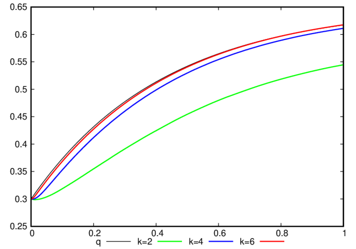
Figure 1: Convergence experiment for a moving front in $(0,1)^{2}$. We compare the true solution $q$ of the sharp interface problem with the discrete approximations $q_{h}$ of the Cahn–Hilliard equation for $\varepsilon=(2^{k}\pi)^{-1}$, $k=2,4,6$.

In order to more closely investigate the convergence behaviour of the phase field solution to the sharp interface solution as $\varepsilon\to 0$, we also compute the error between $q(T)$ and $q_{h}(T)$ at time $T=1$ and display these values in Table 1. The experimential order of convergence suggests a quadratic convergence in $\varepsilon$. This is backed by the fact that the first order correction $\Phi_{1}$, solving (4.11), is zero in the case that the curvature $\kappa$ is zero which holds for a flat interface, see also [23].

$\varepsilon^{-1}$	$|(q-q_{h})(T)|$	EOC
$4\pi$	7.2539e-02	—
$8\pi$	1.9990e-02	1.86
$16\pi$	6.0682e-03	1.72
$32\pi$	1.4667e-03	2.05
$64\pi$	3.3276e-04	2.14

Table 1: Convergence experiment for a moving front in $(0,1)^{2}$, over the time interval $[0,1]$. We also display the experimental order of convergence (EOC).

For completeness, we repeat the same convergence experiment also in three dimensions on the unit cube $\Omega=(0,1)^{3}$. As expected, the observed results are nearly identical to the earlier two-dimensional computations, see Figure 2 and Table 2.

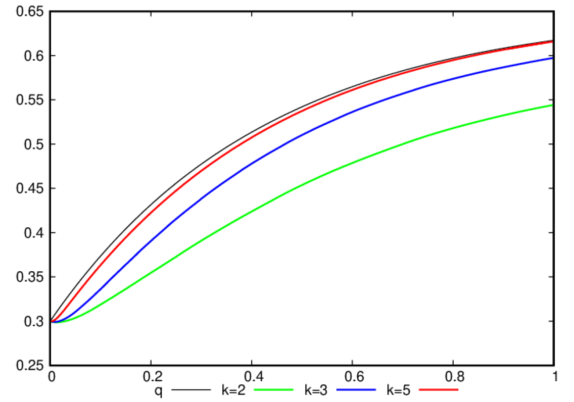
Figure 2: Convergence experiment for a moving front in $(0,1)^{3}$. We compare the true solution $q$ of the sharp interface problem with the discrete approximations $q_{h}$ of the Cahn–Hilliard equation for $\varepsilon=(2^{k}\pi)^{-1}$, $k=2,3,5$.

$\varepsilon^{-1}$	$|(q-q_{h})(T)|$	EOC
$4\pi$	7.2942e-02	—
$8\pi$	1.9824e-02	1.88
$16\pi$	5.8611e-03	1.76
$32\pi$	1.2907e-03	2.18

Table 2: Convergence experiment for a moving front in $(0,1)^{3}$, over the time interval $[0,1]$. We also display the experimental order of convergence (EOC).

For stability investigations, we let $\Omega=(0,1)^{2}$ and set $\beta=0.1$, $S_{\pm}=\mp 8$. This encourages growth of the $2$-mode, as can be seen in Figure 3 for a run with $\varepsilon=\frac{1}{32\pi}$. Here as initial data we use a flat front at the middle of the domain, with an added perturbation of magnitude less than $0.1$ given by a sum of modes from 1 to 20 with random coefficients. Computing the amplification factors in (5.11) shows that ${\widehat{\bm{\ell}}}=(\ell_{2})=(2)$ is the most unstable mode. This agrees with the numerical solution plotted in Figure 3, where the $2$-mode is the one which is most amplified.

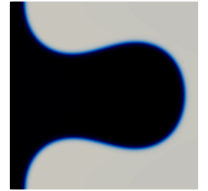
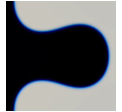
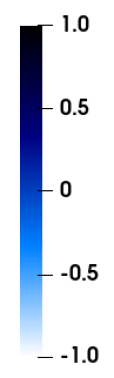
Figure 3: ($\varepsilon=\frac{1}{32\pi}$, $\Omega=(0,1)^{2}$) Evolution for $\beta=0.1$, $S_{-}=8$, $S_{+}=-8$. We show the solution at times $t=0,0.1,1,2,10$.

As an alternative, we compute on $\Omega=(0,4)\times(0,2)$ with $\beta=0.1$, $S_{\pm}=\mp 1.5$. For the same type of initial perturbation as before, this once again encourages growth of the $2$-mode, see Figure 4 for a run with $\varepsilon=\frac{1}{16\pi}$. Also in this case, the linear stability analysis predicts that the $2$-mode is most unstable.

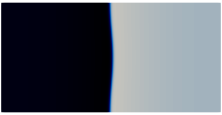
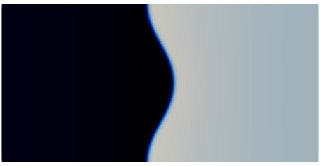
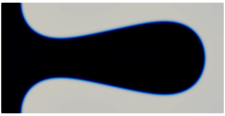
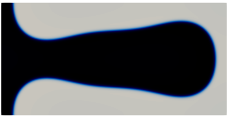
Figure 4: ($\varepsilon=\frac{1}{16\pi}$, $\Omega=(0,4)\times(0,2)$) Evolution for $\beta=0.1$, $S_{-}=1.5$, $S_{+}=-1.5$. We show the solution at times $t=0,1,2,5,10$.

Moreover, on the domain $\Omega=(0,4)\times(0,1)$ we compute with $\beta=0.1$, $S_{\pm}=\mp 3$. See Figure 5 for a simulation with $\varepsilon=\frac{1}{32\pi}$, where we observe the growth of the 1-mode, which is also predicted by the linear stability analysis when computing the numbers for the amplification factors in (5.11) for different values of ${\widehat{\bm{\ell}}}$. At later times the long and nearly horizontal interface becomes unstable for higher modes. Here as initial data we use a flat front at the middle of the domain, with an added perturbation of magnitude less than $0.025$ given by a sum of modes from 1 to 20 with random coefficients.

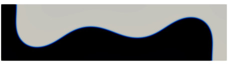
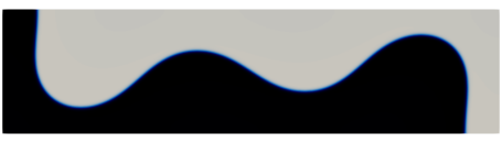
Figure 5: ($\varepsilon=\frac{1}{32\pi}$, $\Omega=(0,4)\times(0,1)$) Evolution for $\beta=0.1$, $S_{-}=3$, $S_{+}=-3$. We show the solution at times $t=0,1,2,5,10$.

Moreover, on the domain $\Omega=(0,2)^{2}$ we compute with $\beta=0.01$, $S_{\pm}=\mp 1.3$. See Figure 6 for a simulation with $\varepsilon=\frac{1}{64\pi}$, where we observe the growth of the 5-mode. Here as initial data we use a flat front at position $0.5$, with an added perturbation of magnitude less than $0.025$ given by a sum of modes from 1 to 20 with random coefficients. It is worth noticing that the 5-mode is also predicted to grow the most by the amplification factors obtained in the linear stability analysis. In this case, we computed the values in (5.11) for a $q(0)$ which leads to a planar solution which is not stationary.

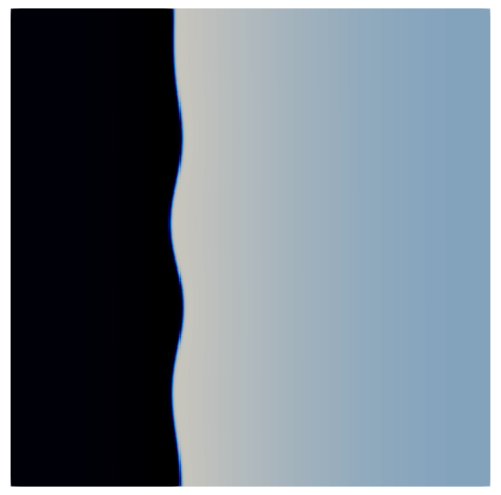
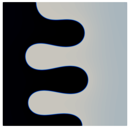
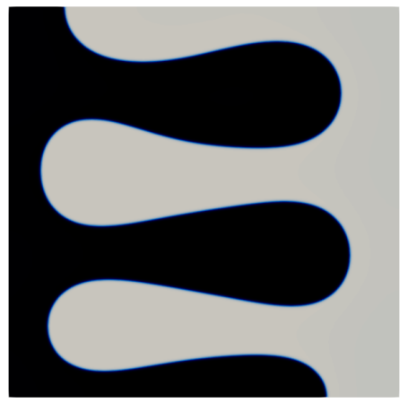
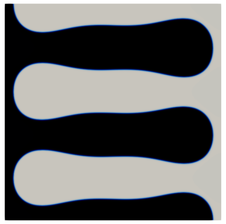
Figure 6: ($\varepsilon=\frac{1}{64\pi}$, $\Omega=(0,2)^{2}$) Evolution for $\beta=0.01$, $S_{-}=1.3$, $S_{+}=1.3$. We show the solution at times $t=0,1,2,3,20$.

For a three-dimensional analogue of Figure 3, we use the parameters $\beta=0.1$, $S_{\pm}=\mp 4.5$, $m_{\pm}=0.2$ on the unit cube $\Omega=(0,1)^{3}$. The initial perturbation of a flat interface at position $q=0.5$ is made up of a single mode with maximal magnitude $0.2$. The evolution is shown in Figure 7.

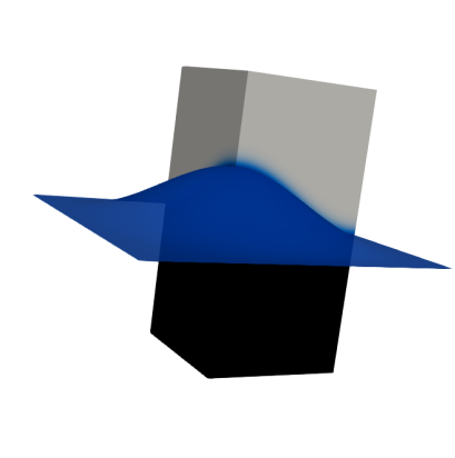
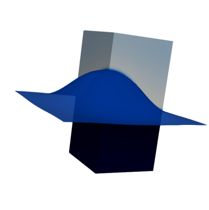
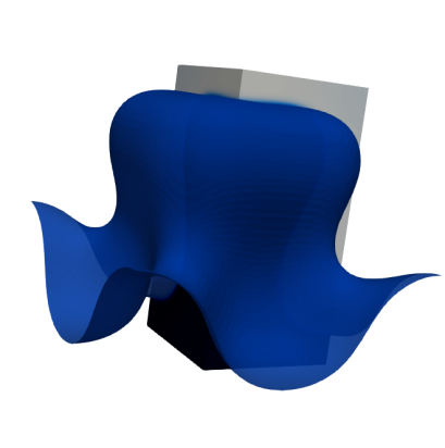
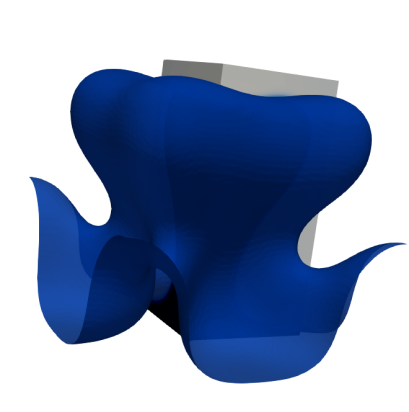
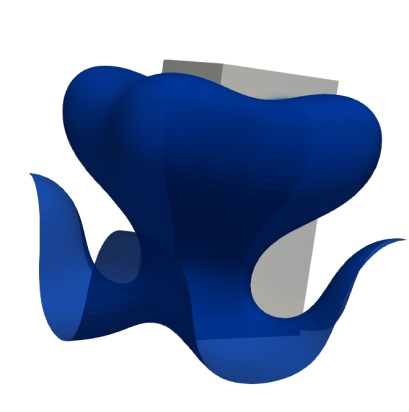
Figure 7: ($\varepsilon=\frac{1}{16\pi}$, $\Omega=(0,1)^{3}$) Evolution for $\beta=0.1$, $m_{\pm}=0.2$, $S_{-}=4.5$, $S_{+}=-4.5$. We show the solution at times $t=0,0.1,0.5,1,1.5$.

6.3 Numerical computations: Spinodal decomposition

In this subsection we are interested in simulations that demonstrate spinodal decomposition. To this end, we choose for the discrete initial data $\varphi_{0}^{h}$ a random function with zero mean and values inside $[-0.1,0.1]$. On the domain $\Omega=(0,4)^{2}$ we then choose the physical parameters $\beta=0.002$, $S_{-}=0.25$, $S_{+}=-4$, and let $\varepsilon=\frac{1}{16\pi}$. The simulation is shown in Figure 8.

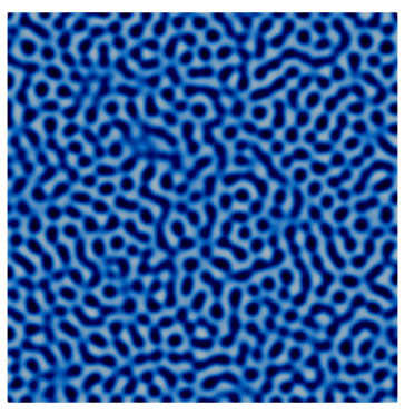
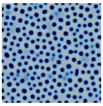
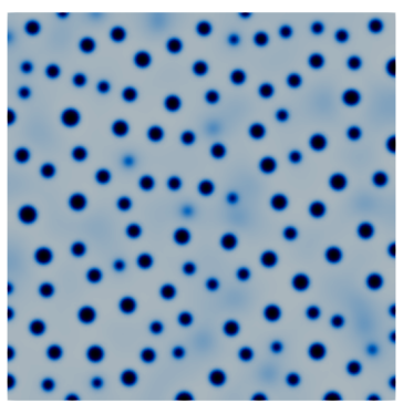
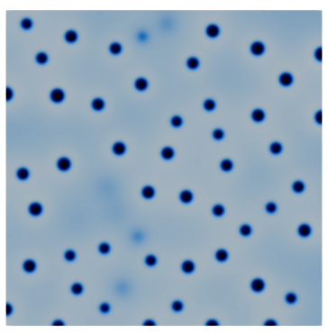
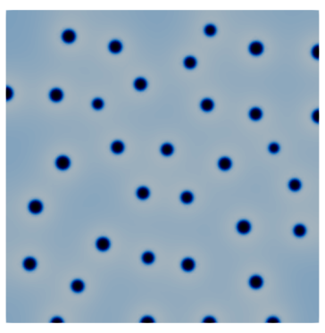
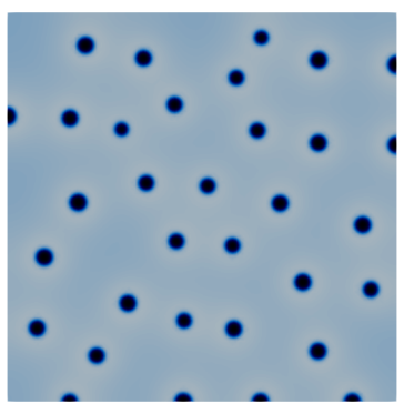
Figure 8: ($\varepsilon=\frac{1}{16\pi}$, $\Omega=(0,4)^{2}$) Evolution for $\beta=0.002$, $S_{-}=0.25$, $S_{+}=-4$. We show the solution at times $t=0.1,0.5,1,2,10,100$. In our numerical computations the solution at the final time appears to be a steady state.

Increasing the value of $\beta$ to $0.02$ yields the results shown in Figure 9.

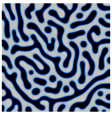
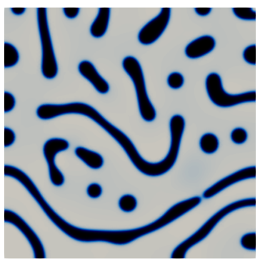
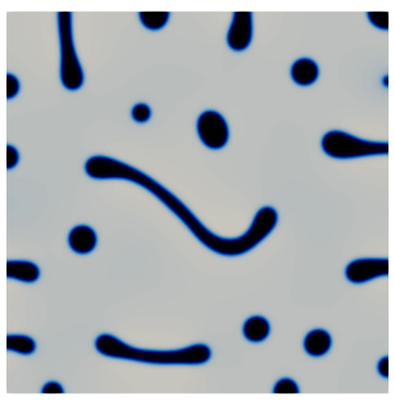
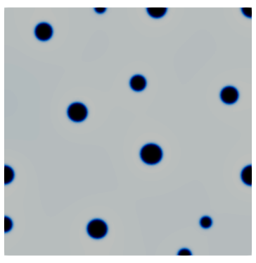
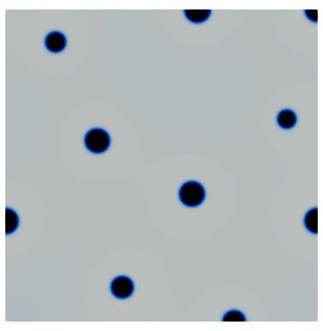
Figure 9: ($\varepsilon=\frac{1}{16\pi}$, $\Omega=(0,4)^{2}$) Evolution for $\beta=0.02$, $S_{-}=0.25$, $S_{+}=-4$. We show the solution at times $t=0.1,0.5,1,2,10,100$. In our numerical computations the solution at the final time appears to be a steady state.

To understand the observed behaviour at the end of the simulations shown in Figures 8 and 9 a bit better, we consider an experiment with the same physical parameters as in Figure 9, but starting from three circular initial blobs with radii $0.29$, $0.3$ and $0.31$. As can be seen from the evolution shown in Figure 10, the three blobs very quickly reduce in size and move apart from each other. Soon after they settle on an arrangement that in our numerical computations is a steady state.

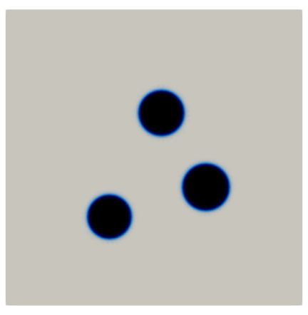
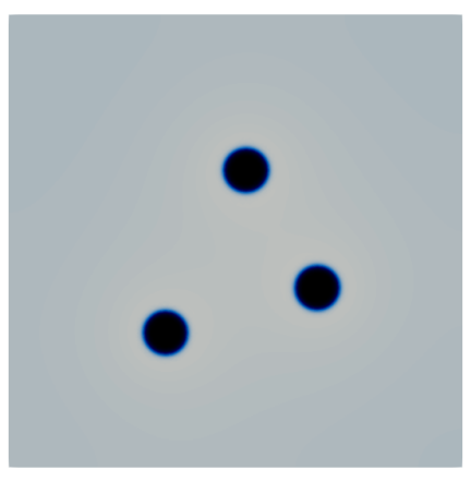
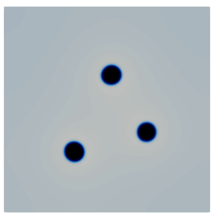
Figure 10: ($\varepsilon=\frac{1}{16\pi}$, $\Omega=(0,4)^{2}$) Evolution for $\beta=0.02$, $S_{-}=0.25$, $S_{+}=-4$. We show the solution at times $t=0,1,10,100$. In our numerical computations the solution at the final time appears to be a steady state.

Next we consider some analogous simulations in 3d. For the simulations in Figures 11, 12 and 13 we let $\Omega=(0,1)^{3}$ and always choose $S_{+}=-4$. For the remaining physical parameters we choose $(\beta,S_{-})=(0.02,0.25),(0.1,0.25),(0.02,1),(0.1,1)$, respectively. For the phase field parameter we choose $\varepsilon=\frac{1}{8\pi}$, and set $\tau=10^{-4}$.

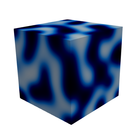
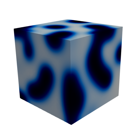
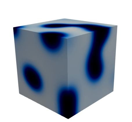
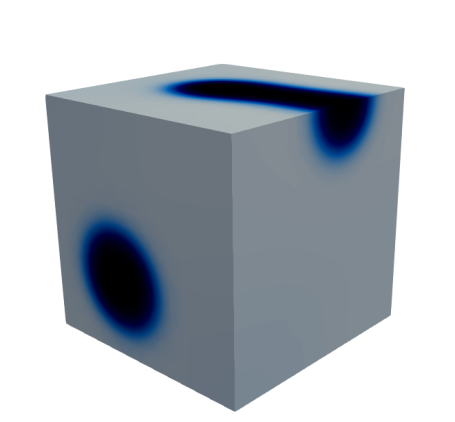
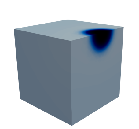
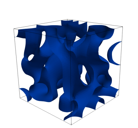
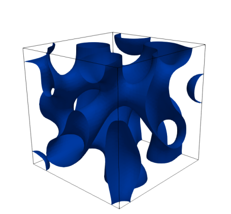
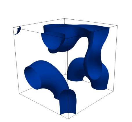
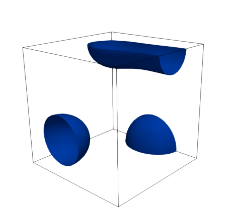
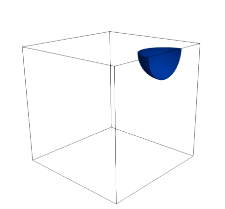
Figure 11: ($\varepsilon=\frac{1}{8\pi}$, $\Omega=(0,1)^{3}$) Evolution for $\beta=0.02$, $S_{-}=0.25$, $S_{+}=-4$. We show the solution at times $t=0.1,0.2,0.5,1,5$.

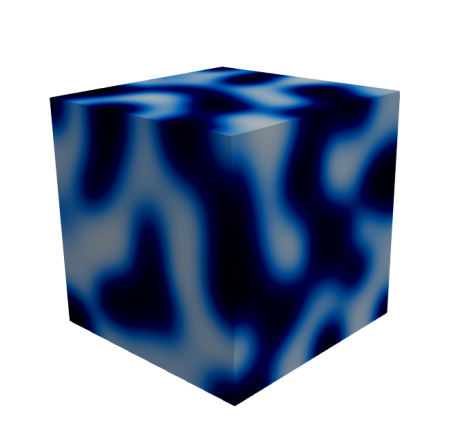
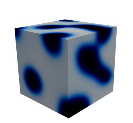
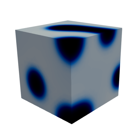
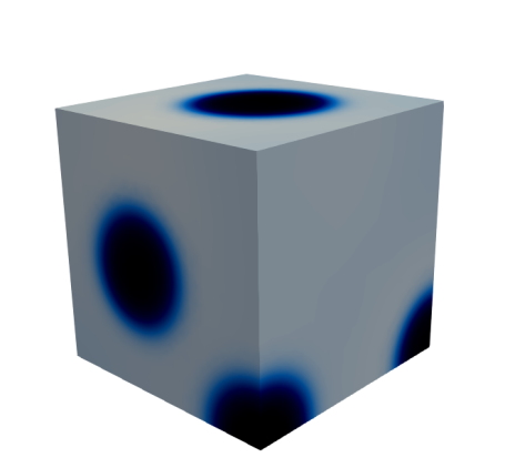
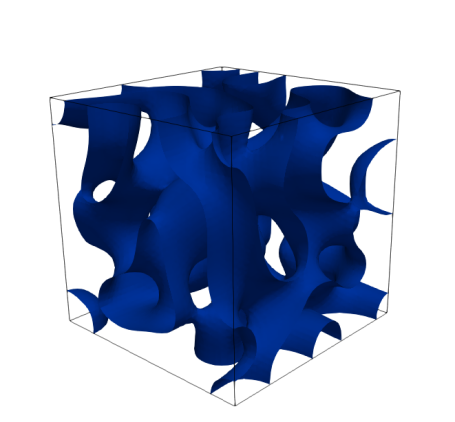
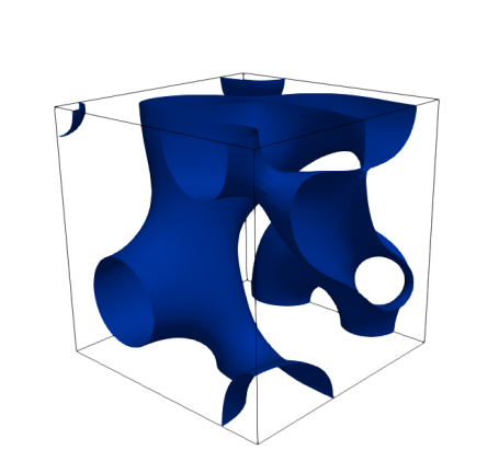
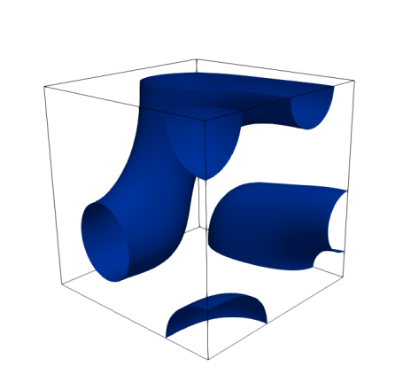
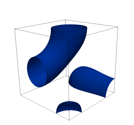
Figure 12: ($\varepsilon=\frac{1}{8\pi}$, $\Omega=(0,1)^{3}$) Evolution for $\beta=0.02$, $S_{-}=1$, $S_{+}=-4$. We show the solution at times $t=0.01,0.05,0.1,0.5,5$.

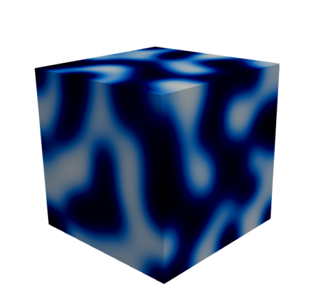
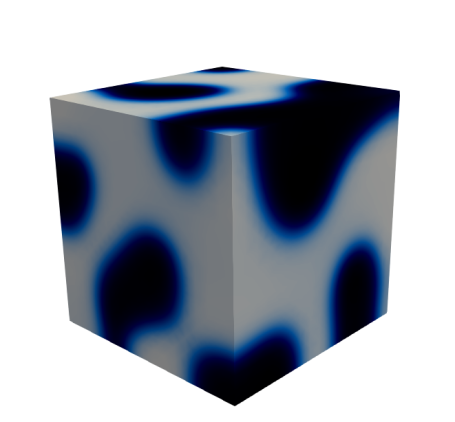
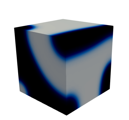
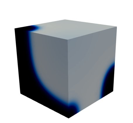
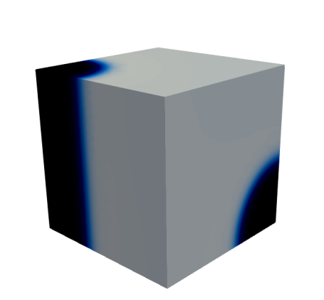
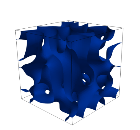
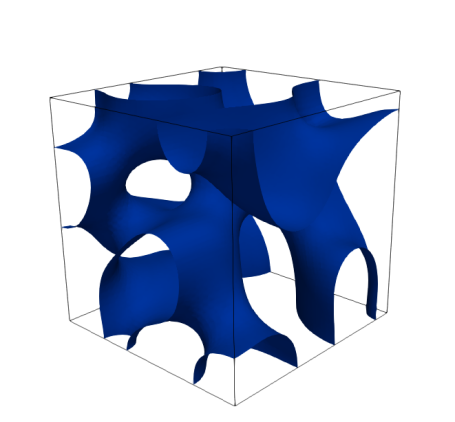
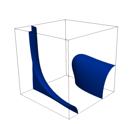
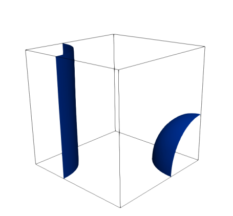
Figure 13: ($\varepsilon=\frac{1}{8\pi}$, $\Omega=(0,1)^{3}$) Evolution for $\beta=0.1$, $S_{-}=1$, $S_{+}=-4$. We show the solution at times $t=0.02,0.1,0.5,1,5$.

For a three-dimensional analogue of Figure 10, we use the parameters $\beta=0.1$, $S_{-}=0.8$, $S_{+}=-10$, $m_{-}=0.2$, $m_{+}=0.5$, $\rho_{\pm}=0.6$, on the cube $\Omega=(0,4)^{3}$. We start from three spherical initial blobs with radii $0.34$, $0.35$ and $0.36$. As can be seen from the evolution shown in Figure 14, the three blobs hardly change their size, and soon settle on an arrangement that in our numerical computations is a steady state. As further coarsening is eventually suppresses these two and three dimensional computations show that the active Cahn–Hilliard model can suppress Ostwald ripening. This is in agreement with [32] which studied the suppression of Ostwald ripening in so-called active emulsions. In particular, multiple droplets can be stable. Due to the Neumann boundary conditions, we can extend the solution obtained by reflections in space and we then observe also the occurrence of cylinders and toroidal shapes.

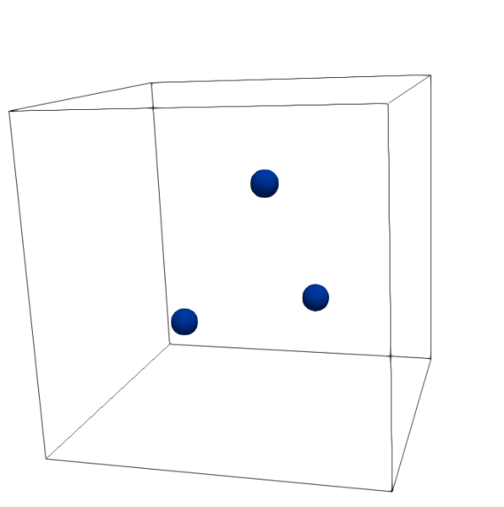
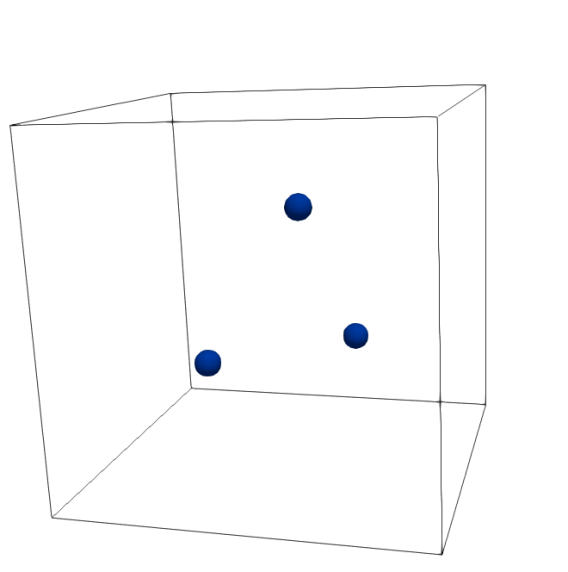
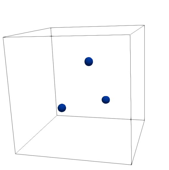
Figure 14: ($\varepsilon=\frac{1}{8\pi}$, $\Omega=(0,4)^{3}$) Evolution for $\beta=0.1$, $S_{-}=0.8$, $S_{+}=-10$, $m_{-}=0.2$, $m_{+}=0.5$, $\rho_{\pm}=0.6$. We show the solution at times $t=0,1,5$. In our numerical computations the solution at the final time appears to be a steady state.

6.4 Numerical computations: Active droplets in 2d

Our first simulation for active droplets shows the possible creation of shells in 2d. We let $\Omega=(0,2)^{2}$ and choose $\beta=0.002$, $S_{-}=0.25$, $S_{+}=-4$ for the physical parameters. The initial droplet is a disk of radius $r_{0}=0.4$. For the phase field parameter we choose $\varepsilon=\frac{1}{32\pi}$. See Figure 15, where we observe the development of a stable shell.

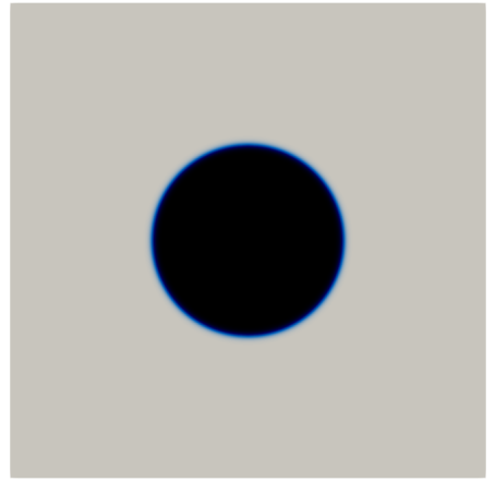
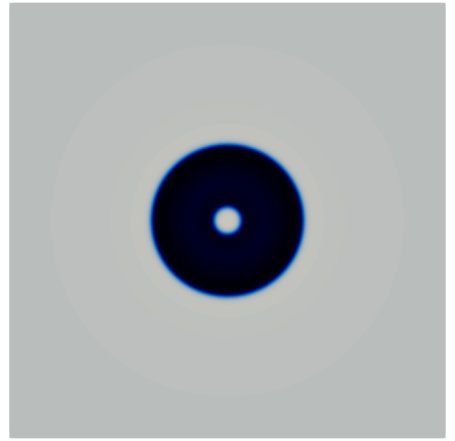
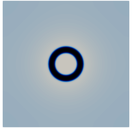
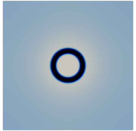
Figure 15: ($\varepsilon=\frac{1}{32\pi}$, $\Omega=(0,2)^{2}$) Evolution for $\beta=0.002$, $S_{-}=0.25$, $S_{+}=-4$. We show the solution at times $t=0,0.2,1,2,5$.

However, if we reduce the dimension of the domain to the unit square, $\Omega=(0,1)^{2}$, then the shell shape is only transient. In fact, the temporary shell evolves to a smaller, stable disk. See Figure 16 for the results.

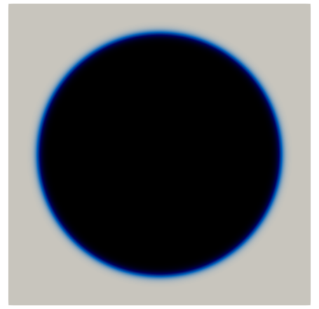
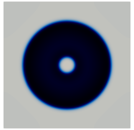
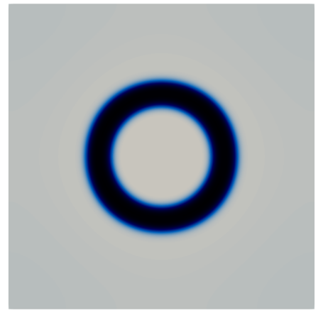
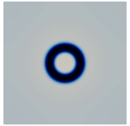
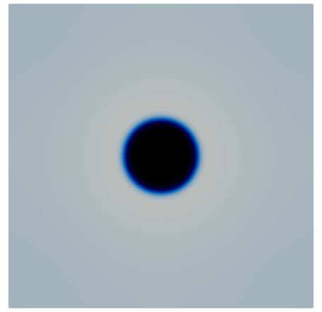
Figure 16: ($\varepsilon=\frac{1}{32\pi}$, $\Omega=(0,1)^{2}$) Evolution for $\beta=0.002$, $S_{-}=0.25$, $S_{+}=-4$. We show the solution at times $t=0,0.2,1,2,5$.

The next simulation shows pinch-off for a slightly perturbed initially circular droplet. In fact, for the “radius” of the initial droplet we choose

$$r_{0}(\theta)=0.25+0.02\cos(2\theta-\tfrac{2\pi}{9}),$$ (6.3)

with $\theta\in[-\pi,\pi]$ denoting the angle in polar coordinates. Hence the initial blob has its widest dimension along an axis that is tilted by $20^{\circ}$ compared to the $x$-axis, with the smallest dimension along an axis perpendicular to it. Letting this initial droplet evolve in the domain $\Omega=(0,2)^{2}$ leads to a thinning of the droplet at the centre of the domain, and eventually to a pinch-off into two separate droplets. See Figure 17 for our numerical results for $\varepsilon=\frac{1}{16\pi}$.

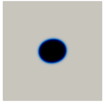
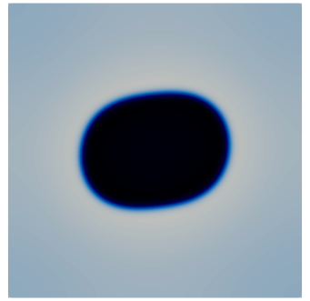
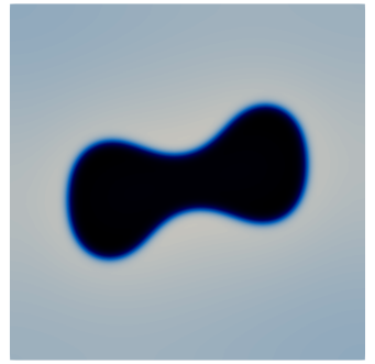
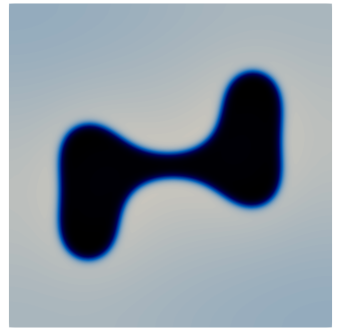
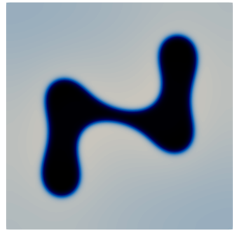
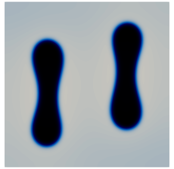
Figure 17: ($\varepsilon=\frac{1}{16\pi}$, $\Omega=(0,2)^{2}$) Evolution for $\beta=0.02$, $S_{-}=1$, $S_{+}=-4$. We show the solution at times $t=0,2,4,6,8,10$.

Running the simulation on the larger domain $\Omega=(0,8)^{2}$ once again shows very delicate fingering patterns appear, but no pinch-off occurs. See Figure 18.

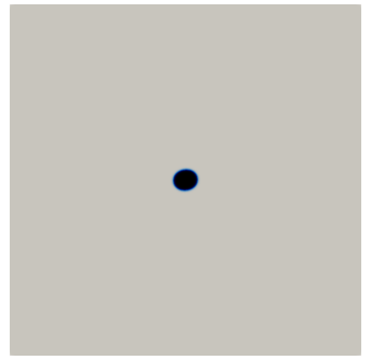
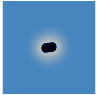
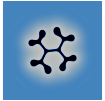
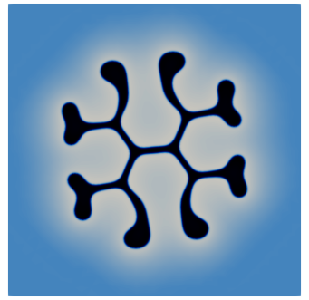
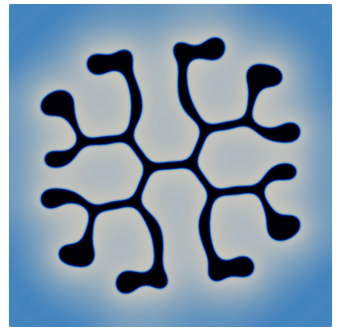
Figure 18: ($\varepsilon=\frac{1}{16\pi}$, $\Omega=(0,8)^{2}$) Evolution for $\beta=0.02$, $S_{-}=1$, $S_{+}=-4$. We show the solution at times $t=0,2,4,6,8,10$.

6.5 Numerical computations: Active droplets in 3d

In our first simulations for active droplets in 3d, we attempt to create analogous shell structures as in Figure 15. To this end, we let $\Omega=(0,2)^{3}$ and choose the same physical parameters $\beta=0.002$, $S_{-}=0.25$, and $S_{+}=-4$. The initial droplet is a ball of radius $r_{0}=0.4$. For the phase field parameter we choose $\varepsilon=\frac{1}{16\pi}$. See Figure 19, where we observe the creation of a shell, which eventually changes into a single ball again.

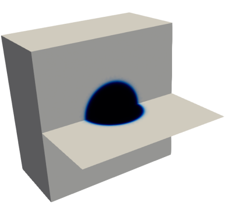
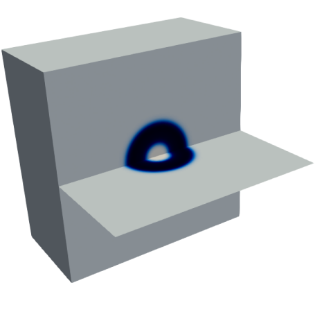
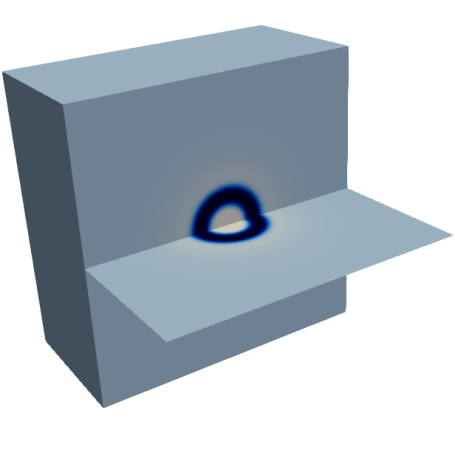
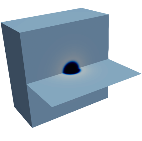
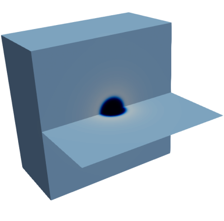
Figure 19: ($\varepsilon=\frac{1}{16\pi}$, $\Omega=(0,2)^{3}$) Evolution for $\beta=0.002$, $S_{-}=0.25$, $S_{+}=-4$. We show the solution at times $t=0,0.3,1,2,5$.

When we increase the radius of the initial ball to $r_{0}=0.6$, then the ensuing evolution is more intricate, see Figure 20. At first two concentric shells appear, with the inner shell merging into a ball after some time. Then the inner ball disappears, leaving just a thin outer shell, which starts to become thinner and thinner, and which eventually fragments into several much smaller blobs. These blobs become spherical and then continue to move away from each other, slowly increasing in size.

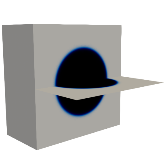
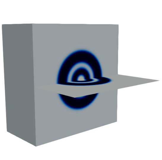
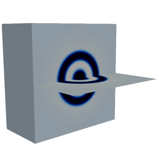
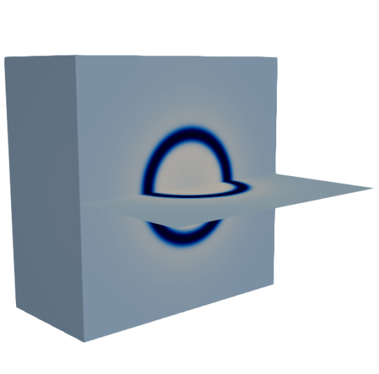
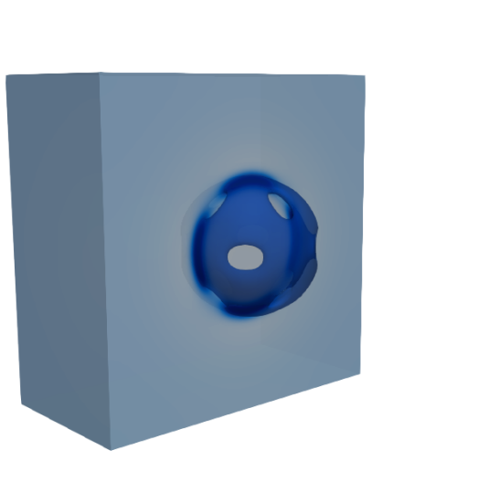
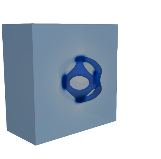
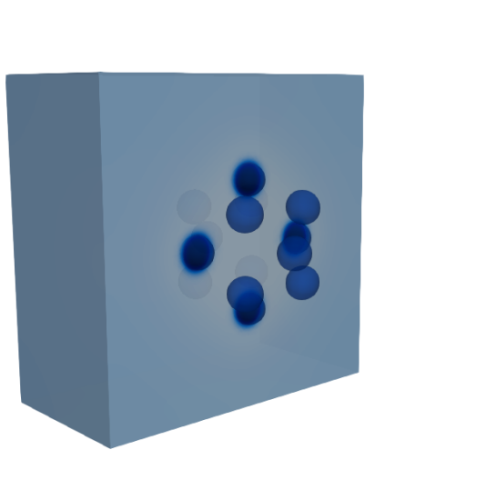
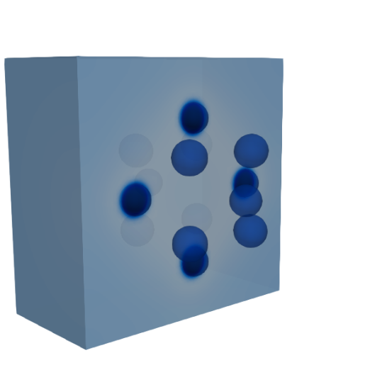
Figure 20: ($\varepsilon=\frac{1}{16\pi}$, $\Omega=(0,2)^{3}$) Evolution for $\beta=0.002$, $S_{-}=0.25$, $S_{+}=-4$. We show the solution at times t = 0, 0.3, 0.5, 1, 1.5, 1.6, 2, 5 where the visualizations in the two rows differ.

For the remaining experiments in this subsection we use $r_{c}=0.5$, recall (2.3), and consider the domain $\Omega=(0,8)^{3}$. In our first experiment, we choose for the initial droplet we choose a rounded cylinder of total dimension $0.8\times 0.4\times 0.4$. In particular, it is made up of two half-balls of radius $0.2$, which are connected with a cylinder of radius $0.2$ and height $0.4$. For the physical parameters we choose $\beta=0.1$, $S_{-}=0.8$, $S_{+}=-10$, $m_{-}=0.2$, $m_{+}=0.5$, $\rho_{-}=0.2$, $\rho_{+}=0.1$, $L=-1$, and we let $\varepsilon=\frac{1}{16\pi}$. The results of our numerical simulation can be seen in Figure 21, where we notice a primary pinch-off that then leads to several secondary pinch-offs.

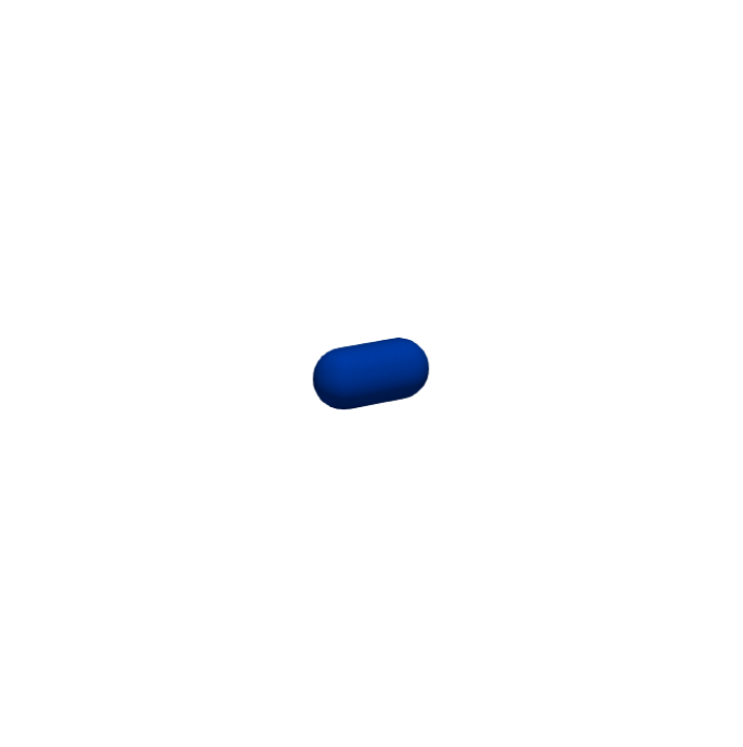
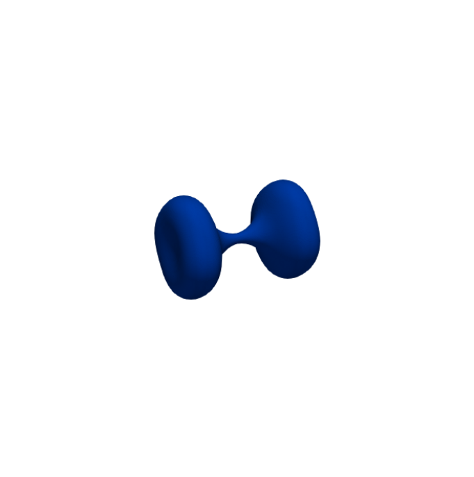
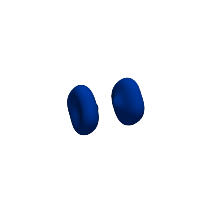
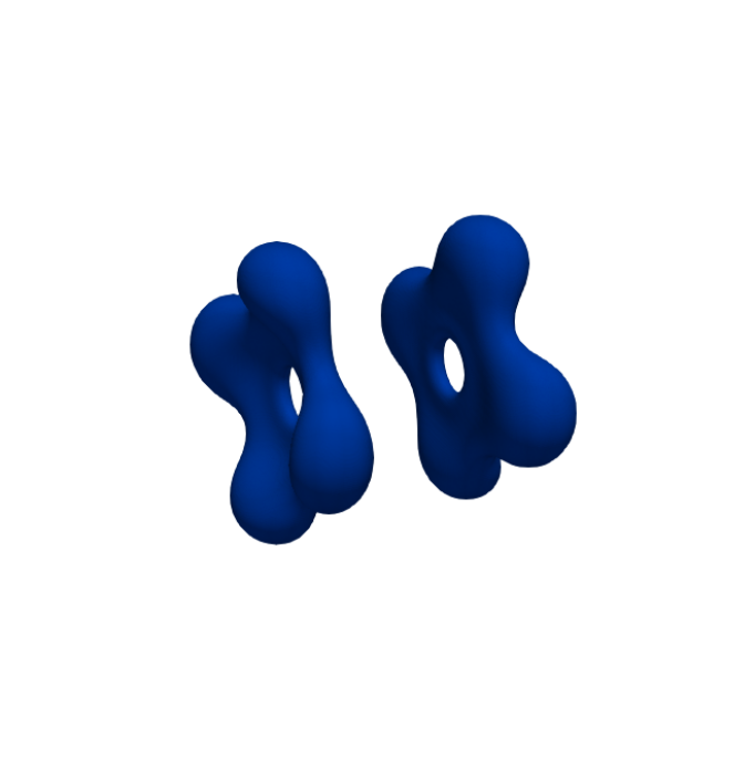
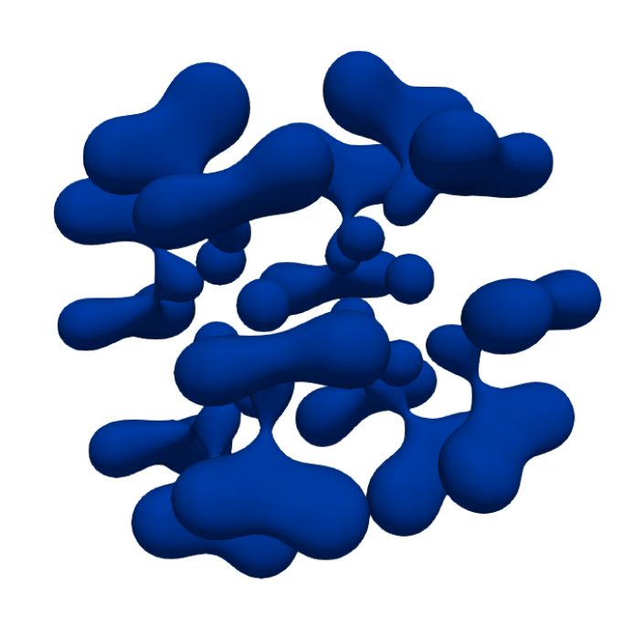
Figure 21: ($\varepsilon=\frac{1}{16\pi}$, $\Omega=(0,8)^{3}$) Evolution for $\beta=0.1$, $S_{-}=0.8$, $S_{+}=-10$, $m_{-}=0.2$, $m_{+}=0.5$, $\rho_{-}=0.2$, $\rho_{+}=0.1$, $L=-1$. We show the solution at times $t=0,1,1.3,1.4,2,3.5$.

For the next experiment we only change the aspect ratio of the initial droplet. In particular, the initial droplet now is a a rounded cylinder of total dimension $0.6\times 0.4\times 0.4$. The results of this numerical simulation can be seen in Figure 22. In Figure 23 we show the interfaces at time $t=4.4$ within $\Omega$ from three different points of view. We observe that the evolution can be very complex with many splittings and other topological changes. Figure 23 shows that droplets have been formed in the center and away from the center the evolution is still very complex. We expect that eventually more and more round droplets will form.

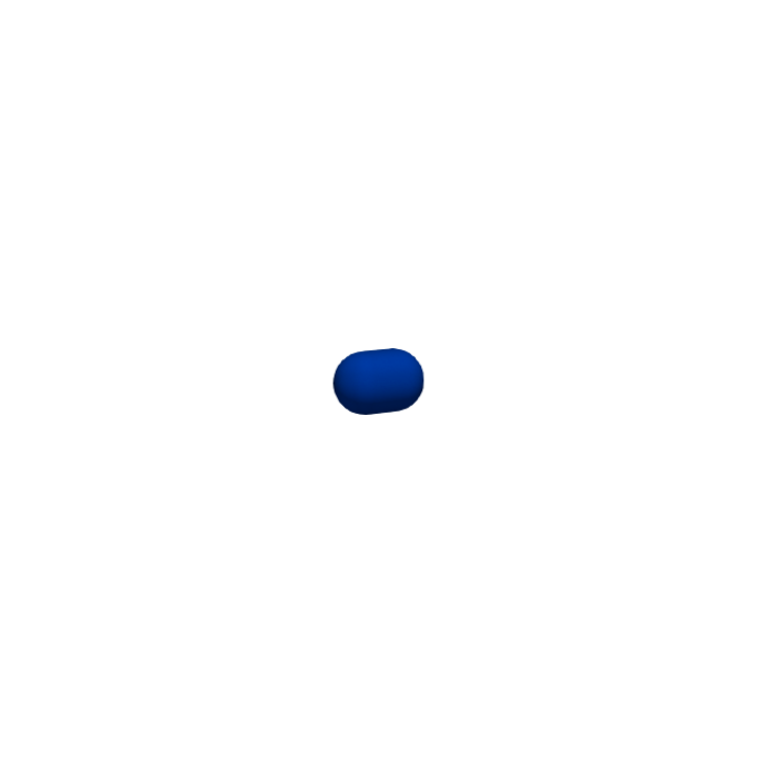
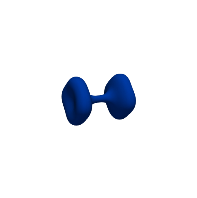
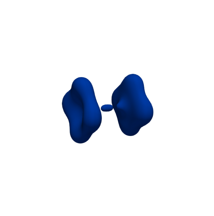
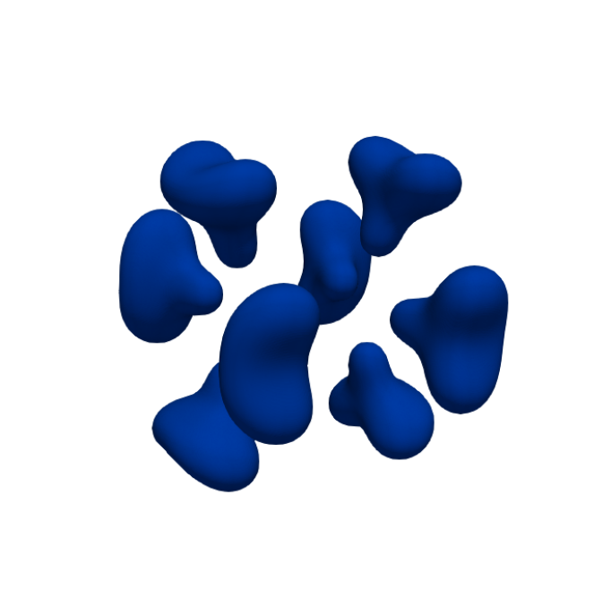
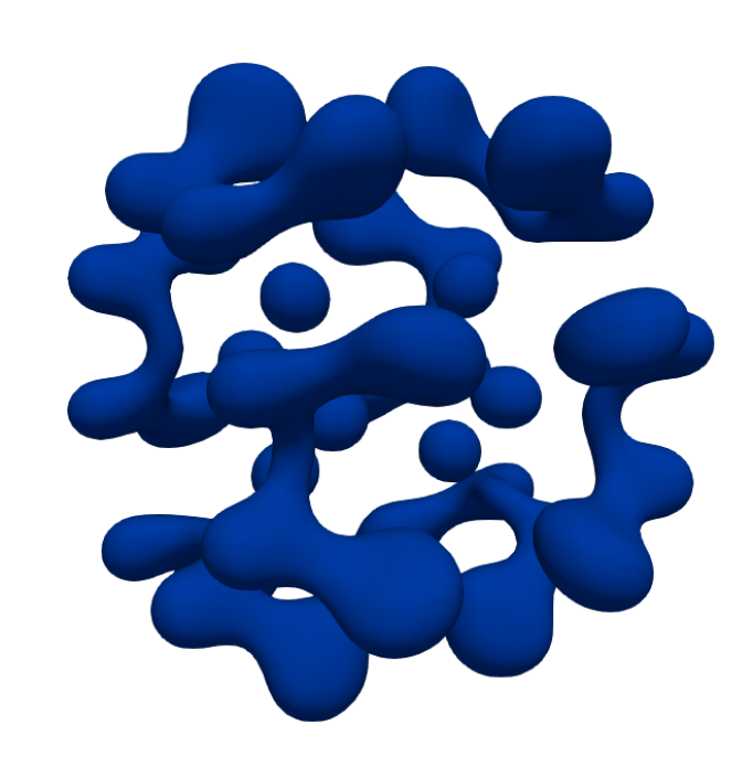
Figure 22: ($\varepsilon=\frac{1}{16\pi}$, $\Omega=(0,8)^{3}$) Evolution for $\beta=0.1$, $S_{-}=0.8$, $S_{+}=-10$, $m_{-}=0.2$, $m_{+}=0.5$, $\rho_{-}=0.2$, $\rho_{+}=0.1$, $L=-1$. We show the solution at times $t=0,1.4,1.8,2,3,4$.

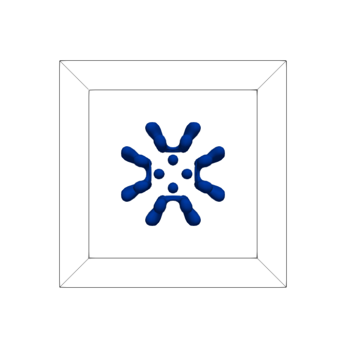
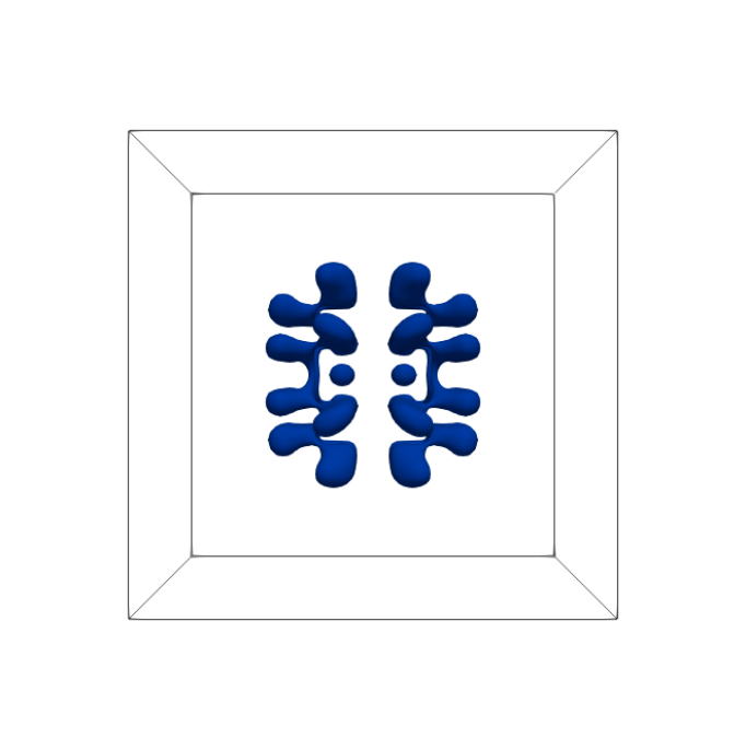
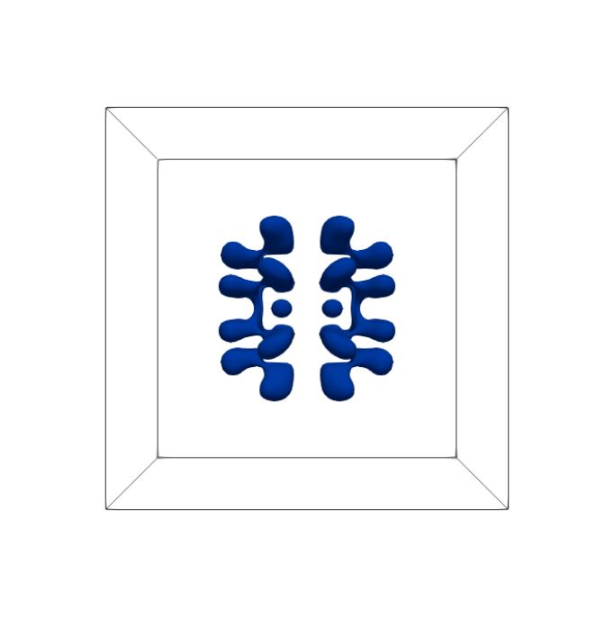
Figure 23: The evolution from Figure 22 at time $t=4.4$ viewed from the front, from the side and from above.

References

- [1] H. Abels, H. Garcke, and G. Grün. Thermodynamically consistent, frame indifferent diffuse interface models for incompressible two-phase flows with different densities. Math. Models Methods Appl. Sci., 22(3):1150013, 2012.
- [2] H. Abels and M. Wilke. Convergence to equilibrium for the Cahn–Hilliard equation with a logarithmic free energy. Nonlinear Anal., 67(11):3176–3193, 2007.
- [3] N. D. Alikakos, P. W. Bates, and X. Chen. Convergence of the Cahn–Hilliard equation to the Hele–Shaw model. Arch. Rational Mech. Anal., 128(2):165–205, 1994.
- [4] E. Bänsch, K. Deckelnick, H. Garcke, and P. Pozzi. Interfaces: modeling, analysis, numerics, volume 51 of Oberwolfach Seminars. Birkhäuser/Springer, Cham, [2023] ©2023.
- [5] J. W. Barrett, R. Nürnberg, and V. Styles. Finite element approximation of a phase field model for void electromigration. SIAM J. Numer. Anal., 42(2):738–772, 2004.
- [6] J. Bauermann, G. Bartolucci, J. Boekhoven, C. A. Weber, and F. Jülicher. Formation of liquid shells in active droplet systems. Phys. Rev. Res., 5(4):043246, 2023.
- [7] L. Baňas and R. Nürnberg. Finite element approximation of a three dimensional phase field model for void electromigration. J. Sci. Comp., 37(2):202–232, 2008.
- [8] A. Bergmann, J. Bauermann, G. Bartolucci, C. Donau, M. Stasi, A.-L. Holtmannspötter, F. Jülicher, C. Weber, and J. Boekhoven. Liquid spherical shells are a non-equilibrium steady state of active droplets. Nat. Commun., 14:6552, 2023.
- [9] A. L. Bertozzi, S. Esedoḡlu, and A. Gillette. Inpainting of binary images using the Cahn–Hilliard equation. IEEE Trans. Image Process., 16(1):285–291, 2007.
- [10] M. Burger, L. He, and C.-B. Schönlieb. Cahn–Hilliard inpainting and a generalization for grayvalue images. SIAM J. Imaging Sci., 2(4):1129–1167, 2009.
- [11] J. W. Cahn. On spinodal decomposition. Acta Metall., 9(9):795–801, 1961.
- [12] J. W. Cahn and J. E. Hilliard. Free energy of a non-uniform system. I. Interfacial free energy. J. Chem. Phys., 28(2):258–267, 1958.
- [13] P. G. Ciarlet. The Finite Element Method for Elliptic Problems. North-Holland Publishing Co., Amsterdam, 1978. Studies in Mathematics and its Applications, Vol. 4.
- [14] V. Cristini, X. Li, J. S. Lowengrub, and S. M. Wise. Nonlinear simulations of solid tumor growth using a mixture model: invasion and branching. J. Math. Biol., 58(4-5):723–763, 2009.
- [15] T. A. Davis. Algorithm 832: UMFPACK V4.3—an unsymmetric-pattern multifrontal method. ACM Trans. Math. Software, 30(2):196–199, 2004.
- [16] C. Donau, F. Späth, M. Sosson, B. A. Kriebisch, F. Schnitter, M. Tena-Solson, H.-S. Kang, E. Salibi, M. Sattler, H. Mutschler, and J. Boekhoven. Active coacervate droplets as a model for membraneless organelles and protocells. Nat. Commun., 11:5167, 2020.
- [17] C. M. Elliott and H. Garcke. On the Cahn–Hilliard equation with degenerate mobility. SIAM J. Math. Anal., 27(2):404–423, 1996.
- [18] C. M. Elliott and S. Zheng. On the Cahn–Hilliard equation. Arch. Rational Mech. Anal., 96(4):339–357, 1986.
- [19] H. Garcke. Curvature driven interface evolution. Jahresber. Dtsch. Math.-Ver., 115(2):63–100, 2013.
- [20] H. Garcke, K. F. Lam, E. Sitka, and V. Styles. A Cahn–Hilliard–Darcy model for tumour growth with chemotaxis and active transport. Math. Models Methods Appl. Sci., 26(06):1095–1148, 2016.
- [21] H. Garcke, K. F. Lam, and V. Styles. Cahn–Hilliard inpainting with the double obstacle potential. SIAM J. Imaging Sci., 11(3):2064–2089, 2018.
- [22] H. Garcke, B. Niethammer, M. Rumpf, and U. Weikard. Transient coarsening behaviour in the Cahn–Hilliard model. Acta Mater., 51(10):2823–2830, 2003.
- [23] H. Garcke and B. Stinner. Second order phase field asymptotics for multi-component systems. Interfaces Free Bound., 8(2):131–157, 2006.
- [24] A. Hawkins-Daarud, K. G. van der Zee, and J. T. Oden. Numerical simulation of a thermodynamically consistent four-species tumor growth model. Int. J. Numer. Methods Biomed. Eng., 28(1):3–24, 2012.
- [25] E. Khain and L. M. Sander. Generalized Cahn–Hilliard equation for biological applications. Phys. Rev. E, 77:051129, May 2008.
- [26] A. Miranville. The Cahn–Hilliard equation, volume 95 of CBMS-NSF Regional Conference Series in Applied Mathematics. Society for Industrial and Applied Mathematics (SIAM), Philadelphia, PA, 2019. Recent advances and applications.
- [27] A. Novick-Cohen. The Cahn–Hilliard equation: mathematical and modelling perspectives. Adv. Math. Sci. Appl., 8:965–985, 1998.
- [28] R. L. Pego. Front migration in the nonlinear Cahn–Hilliard equation. Proc. Roy. Soc. London Ser. A, 422(1863):261–278, 1989.
- [29] A. Schmidt and K. G. Siebert. Design of Adaptive Finite Element Software: The Finite Element Toolbox ALBERTA, volume 42 of Lecture Notes in Computational Science and Engineering. Springer-Verlag, Berlin, 2005.
- [30] W. Yang, Z. Huang, and W. Zhu. Image Segmentation using the Cahn–Hhilliard equation. J. Sci. Comput., 79(2):1057–1077, 2019.
- [31] D. Zwicker, R. Seyboldt, C. A. Weber, A. A. Hyman, and F. Jülicher. Growth and division of active droplets provides a model for protocells. Nat. Phys., doi:10.1038/nphys3984:1745–2481, Dec 2016.
- [32] J. F. Zwicker D, Hyman AA. Suppression of Ostwald ripening in active emulsions. Phys. Rev. E Stat. Nonlin. Soft Matter Phys., 92(1):012317, 2015.