The turnpike control in stochastic multi-agent dynamics: a discrete-time approach with exponential integrators
Abstract
In this manuscript, we study the turnpike property in stochastic discrete-time optimal control problems for interacting agents. Extending previous deterministic results, we show that the turnpike effect persists in the presence of noise under suitable dissipativity and controllability conditions. To handle the possible stiffness in the system dynamics, we employ for the time discretization, integrators of exponential type. Numerical experiments validate our findings, demonstrating the advantages of exponential integrators over standard explicit schemes and confirming the effectiveness of the turnpike control even in the stochastic setting.
keywords:
turnpike property, time-discrete systems, stochastic multi-agent systems, optimal control, exponential integrators[L]
[1]organization=Department of Computer Science, University of Verona,addressline=Strada Le Grazie, 15, postcode=37134, city=Verona, country=Italy \affiliation[2]organization=Istituto Nazionale di Alta Matematica, addressline=Piazzale Aldo Moro, 5, postcode=00185, city=Roma, country=Italy \affiliation[3]organization=Faculty of Informatics, Universita della Svizzera Italiana – USI , addressline=Via La Santa, 1, postcode=6962, city=Lugano, country=Switzerland
1 Introduction
The collective behavior of interacting agents has been the subject of extensive mathematical research, see, e.g., [8, 9]. These models are typically governed by systems of differential equations that describe various interaction mechanisms, such as attraction and repulsion, as well as control inputs that regulate system behavior. This makes them applicable to a wide range of fields, including biology, engineering, economics, and sociology [16, 23]. Significant attention has been devoted to modeling and analysis, and also the study of control impact for such systems has gained interest more recently [15]. Controlling large-scale, high-dimensional agent-based systems presents several theoretical and computational challenges, which have been addressed using various techniques such as Riccati-based methods [22, 2], moment-driven control [4], and model predictive control (MPC) [6], among others.
A promising approach to efficiently control these complex systems is the so-called turnpike control, which leverages the turnpike property to reduce computational costs while maintaining control effectiveness. In few words, the turnpike phenomenon states that, for sufficiently long time horizons, the optimal control and state remain close to the solution of a corresponding static optimization problem over the majority of the time interval. This property has been widely used to improve computational efficiency in optimal control problems [38] and has played a key role in establishing convergence results for MPC methods [18].
In deterministic settings, the turnpike property has been established for both continuous-time [21] and discrete-time [37, 19, 20] systems. However, real-world applications frequently involve stochastic perturbations, which can significantly impact the system’s long-term behavior and control strategies. In this work, we extend the turnpike analysis to stochastic dynamics [33, 34], addressing the challenges posed by noise in multi-agent systems [31, 5]. Additionally, unlike in [20] where the authors employed the explicit Euler method for the time marching, we use integrators of exponential type [26]. This choice, in particular, allows to effectively handle the inherent stiffness that may arise in the interaction dynamics. Exponential integrators provide improved stability properties compared to standard explicit schemes, making them particularly well-suited for stiff systems, and to the authors’ knowledge they have not been employed in this context yet.
The main contributions of this paper are as follows. First, we establish the turnpike property for stochastic discrete-time optimal control problems governing interacting agents, extending previous deterministic results [21, 20]. Our analysis demonstrates that the turnpike effect persists even in the presence of noise, provided certain dissipativity and controllability conditions are fulfilled. Second, we introduce the use of exponential Rosenbrock integrators for the numerical discretization of the obtained stochastic control problem. To this end, we in particular reformulate the problem in matrix form, which facilitates the application of these integrators. Finally, we conduct a series of numerical experiments to validate our findings. We compare standard explicit and exponential integrator-based discretizations in both controlled and uncontrolled settings, demonstrating that schemes of exponential type exhibit superior stability properties, especially in the presence of stiffness. Moreover, we confirm that the turnpike control strategy remains effective in steering the agents toward the desired asymptotic behavior, even in the stochastic setting.
The remainder of this paper is structured as follows. In Section 2, we introduce the stochastic control problem under consideration, including the system dynamics and cost functional. In Section 3, we present the time discretization using exponential integrators, highlighting their advantages over explicit schemes. Section 4 establishes the turnpike property for the discrete-time stochastic system, leveraging strict dissipativity and cheap control conditions. In Section 5, we provide numerical experiments to validate our findings. Finally, Section 6 concludes the paper and presents possible future interesting developments.
2 Stochastic control problem
As already mentioned in the introduction, the turnpike phenomenon is a significant principle in optimal control theory. In fact, it establishes that during a specific interior subinterval of a given time horizon, the dynamic control strategy can be approximated with arbitrary precision by the solution of a (generally less complex) static optimization problem. This insight greatly reduces the computational effort typically associated with dynamic control strategies.
In our framework, we start by considering the continuous trajectories of the interacting agents. We denote by the position of agent at time , with , and the time interval is defined as . The dynamics of the agents are described by the following stochastic differential equation (SDE)
| (1) |
where the term represents the stochastic noise component, with being standard -dimensional independent Brownian motions. The initial condition for each agent is given by , where is a stochastic variable, accounting for randomness in the initial state distribution. The interaction between agents is mediated by a nonlinear interaction kernel which describes the forces governing their behavior. For further examples and theoretical background, we refer to [7]. The system operates within a well-defined probabilistic framework. Let be a complete probability space, where represents the sample space, is the -algebra of measurable events, and is the probability measure. The stochastic processes , are adapted to the filtration , which represents the natural filtration generated by the Brownian motions. This filtration captures all the information available up to time , ensuring that the evolution of the stochastic processes depends on the past without anticipating future information.
The dynamics of the agents are thus driven by both deterministic controls and the stochastic influences represented by the Brownian motions . The control is applied individually to each agent, with the aim of minimizing a cost functional over a finite time horizon. The control objective is to drive the system towards a desired state while minimizing the associated cost. The latter (to be minimized with respect to the control term) incorporates a tracking term, which measures the deviation of each agent from the desired state , and a regularization term to penalize the magnitude of the control. Specifically, the cost functional, which depends on , is given by
| (2) |
Here, we denote as the Euclidean norm on . The parameter is the regularization parameter penalizing the control effort. Each element corresponds to a specific realization from the sample space, thus describing the inherent randomness of the dynamics.
2.1 Static control problem
We now introduce the static control problem. In this setting, the static state of agent is denoted by , and the static control applied to agent is denoted by . The objective is to minimize the static cost functional
| (3) |
with respect to . The minimization is subject to the equilibrium condition for each agent , representing the static version of the system’s dynamics (1). Notice that an equilibrium point for an SDE is a (stochastic) state where the expectation of the dynamics of the system does not change over time. In particular, this means that at the equilibrium the deterministic part of the dynamics (represented by the drift term in (1)) is null. Clearly, since the underlying equations are SDEs, even at equilibrium the system exhibits randomness. Therefore, we remark that the equilibrium in our context is a statistical state rather than a deterministic one. For our specific case, we obtain
| (4) |
Due to the specific structure of the agent-based dynamics, a solution to the static control problem in (3)–(4) exists but is not unique, due to the dependence on the mean and the stochastic nature of the system. Here, we consider the natural candidate solution
| (5) |
This implies that, at equilibrium, the static state for each agent coincides with the desired state , and no control input is required. Please observe that this specific choice of the static pair in (5) is deterministic.
3 Time discretization using exponential integrators
As already mentioned in the introduction, we are interested in computing an approximate solution to the optimal control problem. The presence of a possibly stiff interaction kernel in the dynamics requires careful treatment from a time integration point of view. Indeed, standard explicit integrators (such as the well-known Euler–Maruyama method, or Runge–Kutta methods in the deterministic case) may be subject to severe time step size restrictions due to the lack of favourable stability properties. To overcome this issue, the research community developed many new techniques and ad-hoc numerical methods. Here, we focus on the employment of the so-called exponential integrators [26], which are explicit time marching schemes that have proven to perform very well in the stiff regime on many classes of problems (see, for instance, the works [14, 11, 30, 12, 10, 3] and [28, 32, 29] specifically for the stochastic setting). In particular, for our purposes we will consider a numerical method in the class of the so-called exponential Rosenbrock schemes [27, 32]. The latter are well-suited for systems of differential equations in which there is no a priori separation of a constant linear stiff part and a non-stiff nonlinear term. This partitioning is required, for instance, to employ the so-called exponential Runge–Kutta methods [25, 29].
For convenience of the reader, we report here the main idea at the basis of the derivation of exponential Rosenbrock integrators in a deterministic autonomous setting (a thorough explanation with full details can be found, e.g., in [27]). The extension to the stochastic framework is given below. Let us consider the following general system of ODEs
| (6) |
and the time discretization for . Here denotes the constant time step size and . Then, we continuously linearize along the numerical solution as
where
| (7) |
are the Jacobian matrix of the flow evaluated at and the remainder, respectively. Now, we express the exact solution of system (6) at time by means of the variation-of-constants formula
A numerical method is then obtained by suitably approximating the integral term in the formula above. In particular, considering the approximation , we get the time marching scheme
| (8) | ||||
This is known as exponential Rosenbrock–Euler method. In formula (8), we introduced the matrix function which satisfies the relation . The efficient computation of the matrix exponential and of the exponential-like function (or their action to vectors) is crucial for an effective employment in practice of the integrator. For this specific task we refer to the works [35, 17, 30, 1, 13], among the others. The exponential Rosenbrock–Euler method is a second-order convergent numerical scheme, it is A-stable by construction (since it integrates exactly linear problems) and it is effective for stiff systems.
A stochastic variant of scheme (8) can be obtained by using similar reasoning, see in particular [32]. In fact, a numerical solution to the system of SDEs
where is the term accounting for the Brownian motions, can be obtained by the so-called stochastic exponential Rosenbrock–Euler method
| (9) |
Here, and is defined in (7). The stochastic Rosenbrock–Euler method is a first order scheme (in strong sense) which is suitable for stiff mmetrstems of SDEs. Notice that if we remove the Brownian motion part from the system, the integrators reduces to the standard exponential Rosenbrock–Euler method (8).
Remark 1.
Scheme (9) generalizes straightforwardly to non-autonomous problems in the form
In fact, by equivalently rewriting the system in autonomous formulation (i.e., introducing an additional variable for the time), applying scheme (9), and employing relations of the function we get the time marching method
| (10) |
Here, we define
and still belongs to the class of the so-called -functions.
Recall that, in our case, we are interested in time integrating
for each agent . In the following, we assume for simplicity of notation , i.e., . This assumption will also be used in the numerical examples later and will remain in effect throughout the entire paper. Then, we can write an equivalent matrix formulation of the problem as
| (11) | ||||
where is the vector containing the position of each agent at time , (with ) is the matrix representing the interactions among agents, (with ), is the vector containing the control for each agent , and is the vector of the Brownian motions. Then, employing (10) we get the time marching
| (12) |
where the element of the matrix is given by
while the -th element of is .
4 The turnpike property for the time-discrete stochastic control problem
In this section, we focus on the turnpike property with interior decay in the context of stochastic control problem for interacting agents, discretized in time using exponential integrators (introduced in Section 3).
In order to study the turnpike property in this setting, we first consider the discretized dynamics in formula (12). Then, to complete the formulation, we must also discretize the cost functional (2). To this aim, we employ a first-order quadrature rule (rectangle left point, in particular). Therefore, the fully discrete optimal control problem, which we denote by , is formulated as
| (13) |
where we recall that approximates (i.e., the position of the -th agent at the -th time step) through the dynamics, and is the control applied at the same agent and step. Additionally, we define the running cost at each time step, which describes the contribution of the state and control at time step to the overall cost functional. This is given by
| (14) |
The running cost measures the deviation of the system from the desired state and penalizes the control effort at each discrete time step . In these terms, the minimization in formula (13) can be written as
Notice that the time-discrete optimization problem (13) depends also on the initial time , the terminal time , and the discretization step size . In the time-discrete setting, we assume that these parameters are chosen so that the number of time steps is given by
| (15) |
where represents the total number of time steps between and . The discrete-time optimization problem thus consists of minimizing the cost functional over time steps. The optimal value of the time-discrete problem is denoted by
where is the initial state of the system, representing the positions of all agents at the initial time .
This formulation captures the time-discrete version of the stochastic control problem, enabling us to apply the turnpike property analysis in the time-discrete setting. In the next steps, we will examine the conditions under which the turnpike property holds for this time-discrete stochastic control problem. Specifically, we will investigate the proximity of the optimal dynamic trajectory to the corresponding static solution, particularly in the interior of the time horizon. In the upcoming analysis, given a state vector in , we consider the norm
This corresponds to the standard Euclidean norm in and will serve as our primary measure of magnitude for the state vector.
4.1 The strict dissipativity property
A key requirement for establishing the turnpike property is the concept of strict dissipativity of the cost functional. This notion, originally introduced in [36], plays a fundamental role in optimal control theory. Dissipativity provides a connection between the system’s dynamics and its cost structure, ensuring that the system’s behavior converges to an optimal steady-state over time. While widely used in continuous-time control systems, here we extend it to the time-discrete setting, focusing on the optimal control problem formulated for interacting agents.
To formalize strict dissipativity in this context, we introduce the key components. The supply rate function measures the deviation of the current state-control pair from the optimal static pair . The storage function , bounded from below acts as an energy-like function capturing the system’s stored cost. The dissipation function , continuous and monotone increasing with , quantifies the rate at which deviations from the optimal steady-state are penalized. In our setting, the supply rate function is chosen as
where is the running cost defined in (14). Since is the optimal static pair minimizing the running cost, we have . Thus, the supply function simplifies to , which directly quantifies how far the system is from the optimal steady-state. To ensure strict dissipativity, we require the existence of a storage function and a dissipation function satisfying a key inequality. Specifically, defining and assuming a control penalization parameter , we ensure that larger deviations from the optimal steady-state incur a greater cost, promoting convergence.
We now present the complete statement of strict dissipativity.
Lemma 4.1.
Let the control penalization parameter . The time-discrete optimal control problem is strictly dissipative with respect to the supply rate function . That is, there exists a storage function , bounded from below, and a continuous, monotone increasing function with , such that for all state-control pairs satisfying the discrete dynamics (12), the following inequality holds in expectation over the noise
| (16) |
Proof.
To establish strict dissipativity, we recall that and the choices and . Then, using these definitions and the properties of the optimal static pair, we derive the following sequence of inequalities
Here we also used the fact that . Finally, since the noise in the system must be taken into account, we incorporate expectations on both sides of the dissipativity inequality. This ensures that the inequality holds on average, accounting for the stochastic nature of the problem. Thus, multiplying both sides by , and choosing , we can write the strict dissipativity condition in the mean sense
This concludes the proof. ∎
Remark that, in our setting, we obtain that the time-discrete optimal control problem satisfies the strict dissipativity property (16) with and . This in particular means that deviations from the static optimal solution are penalized in a way that guarantees convergence to the static optimal pair as the time horizon progresses.
4.2 The cheap control condition
In the pursuit of establishing the turnpike property, we identify the cheap control condition as the second essential ingredient, following the dissipativity condition we explored earlier. While the dissipativity condition ensures that the system’s behavior remains well-defined and controllable, the cheap control assumption introduces a crucial bound that relates to the distance between the initial state and the steady-state solution of the time-discrete problem. The combination of these two properties will ultimately facilitate our analysis of the turnpike phenomenon.
The cheap control condition asserts that the cost required to steer the system from an initial state to the steady-state solution remains bounded by a function of the initial deviation and a term related to storage function differences. This condition provides a measure of how efficiently the system can be controlled and ensures that the overall control effort remains manageable. To properly set up the framework, we introduce the following assumption.
Assumption 4.2.
We assume that the interaction kernel in (1) is bounded, i.e., there exists a constant such that
The boundedness of the kernel ensures that the interaction effects remain controlled and do not grow unreasonably large. This assumption is important for guaranteeing stability in the system’s dynamics and facilitating the analysis of control strategies, even in cases where the interactions may be asymmetric. We now present the formal statement of the cheap control condition.
Lemma 4.3.
Under Assumption 4.2, the optimal control problem is cheaply controllable, that is, there exist constants and such that for all initial times , all initial states , and for all terminal times , the following inequality holds
| (17) |
Proof.
We prove the cheap controllability condition with . As in the proof of Lemma 4.1, we select and . Then, with these choices, to establish the validity of inequality (17), we need to prove that there exists a constant such that for all initial times , terminal times , and initial states , the following relationship holds
To prove it, we can leverage a stabilizing feedback control law, similar to the one discussed in [21], which accommodates the stochastic dynamics of the system. This feedback mechanism is pivotal as it facilitates the exponential decay of the running cost defined in (14). Let us consider a parameter . For each agent and time step , we define the cheap control input as follows
| (18) |
The corresponding state evolves from any initial state in accordance with the scheme described by (12), using the mean control strategy in (18). Observe that at this stage we use the autonomous version of scheme (12) (in particular ), because the control in (18) does not depend on time. If we substitute the control law (18) into the stochastic dynamics (1) and we take the expectation on both sides (since our focus is on the mean evolution of the agents’ states), after simple calculations we obtain the following
| (19) |
Applying now the stochastic exponential Rosenbrock–Euler method we get
| (20) |
where we defined . Notice that in (19) where we are dealing with the mean dynamics, the stochastic exponential Rosenbrock–Euler method effectively coincides with the standard exponential Rosenbrock–Euler method. This is because, in the evolution of the mean, the uncertainty introduced by the noise term disappears, as the expectation of the Brownian motion is zero. Then, we are left with a purely deterministic evolution for the mean. Furthermore, since the exponential Rosenbrock–Euler method is exact for linear equations (and (19) is linear), the numerical scheme (20) is not just an approximation, but actually represents the exact solution to the mean dynamics. This is not true, e.g., if we employ a standard explicit method as explicit Euler.
To measure how close the system is to the static state, we introduce the quadratic Lyapunov function
Using (20), the evolution of this function is governed by the following recurrence
Expanding this expression, we get
This shows that the Lyapunov function decays exponentially at each time step. Thus, for all ,
Now, starting from the cheap control (18), we apply the triangle inequality and we use the boundedness of in Assumption 4.2:
We remind that we indicate . Next, squaring both sides and applying the inequality , as well as the Cauchy-Schwarz inequality as , we get:
Summing over we obtain:
Defining the positive constant , we obtain
We can then bound the total cost
Substituting the exponential decay of , we obtain
Since the series converges, we can write
where
is a constant that depends on the control parameters. This concludes the proof. ∎
4.3 The turnpike property with interior decay
In this section, we establish the turnpike property with interior decay. We recall that this concept highlights that the optimal solution of a dynamic optimal control problem remains close to the corresponding static optimal solution for most of the time interval, provided the time horizon is sufficiently large.
Our main final result is the following (Theorem 4.4), which will be proven by leveraging the dissipativity inequality established earlier and the property of cheap controllability.
Theorem 4.4.
Proof.
We recall that, under the assumptions, the problem fulfills the strict dissipativity inequality (16) and it is cheaply controllable (17) for and Let now represent the optimal state and control for the problem . Using the dissipativity inequality and the property of cheap control, we derive
| (21) | ||||
Define
with . Then, there exists an index for which the following inequality is satisfied
| (22) |
Indeed, by contradiction assume that for all , the inequality
is valid. Then, it would imply
contradicting (21). Therefore, we get
| (23) | ||||
The value is the optimal cost for the problem initialized at with state . Using the cheap control result (Lemma 4.3), we have
| (24) |
Combining (22) with (24), exploiting that is monotone increasing, we find
Finally, substituting this into (23) gives
We now define the -dependent constant as
This completes the proof. ∎
4.4 Estimation of the turnpike time
The turnpike time corresponds to the time after which the cheap control can be switched off and replaced with the static control. To determine the turnpike time theoretically, we leverage the decay of the Lyapunov functional. Recall that the Lyapunov functional is defined as
and its evolution at each time step is given by
Thus, for all , the decay can be expressed explicitly as
To estimate , we impose a threshold that quantifies how close the system state should be to the target state . Specifically, we require
which, using the decay expression, translates to
Dividing by and taking the natural logarithm, we obtain
Therefore, we conclude that the turnpike time may be taken as
| (25) |
This theoretical estimate provides a systematic way to determine based on the parameters , the expectation of the initial state , the target state , and the desired threshold . By selecting an appropriate , one can identify the time at which the cheap control can be replaced by the static control.
5 Numerical experiments
We now present several numerical experiments that demonstrate the theoretical findings of the previous sections and show the advantage of employing exponential integrators in our context. In all tests, we assume that the number of agents is and that they start uniformly distributed in the interval . The starting point of the time horizon is , while the final simulation time is set to . To model the interactions, if not differently specified, we employ a Cucker–Smale-like kernel of the form
| (26) |
with . Notice that the stiffness in the interaction kernel is essentially controlled by the magnitude of the parameter , which changes depending on the specific example under consideration. Concerning the stochastic noise component in (1), if present, we set . Also, the number of Brownian motion paths considered for the numerical simulations is .
We compare the stochastic exponential Rosenbrock–Euler method (9) with the well-known Euler–Maruyama method [24]. For the system under consideration, i.e., problem (11), we recall that this method marches as
| (27) |
All the numerical experiments have been performed with MathWorks MATLAB® R2022a on an Intel® Core™ i7-10750H CPU (six physical cores) equipped with 16GB of RAM. To compute the needed functions in the exponential integrators, we employ a Padé approximation with modified scaling and squaring [35].
5.1 Examples with no control in the dynamics
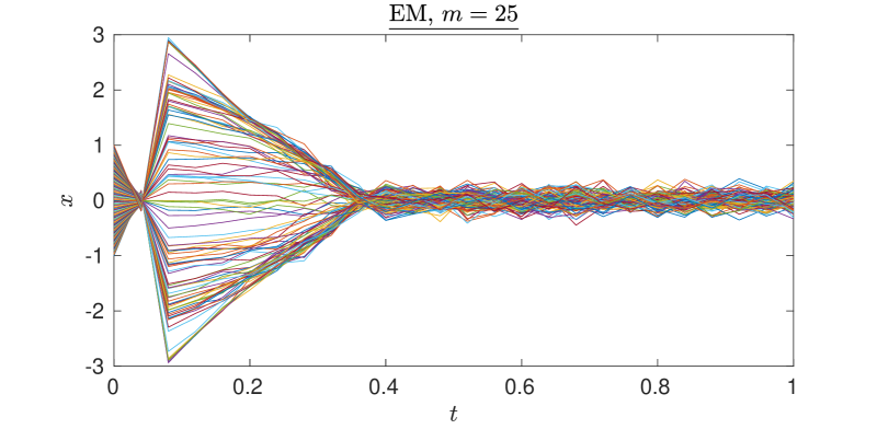
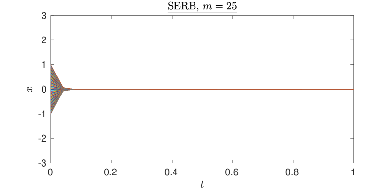
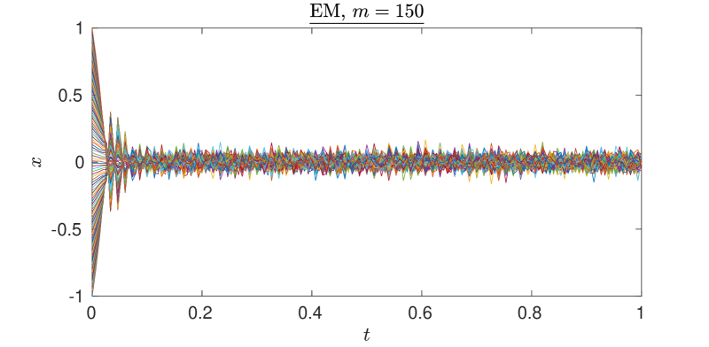
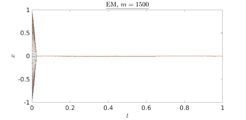
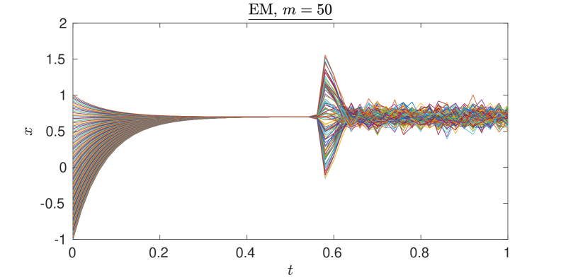
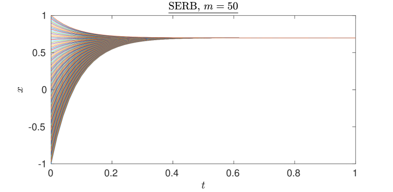
The first test that we perform corroborates the assertion that standard explicit methods (the Euler–Maruyama scheme (27), in particular) do require a time step size restriction when the interaction kernel is stiff, while the stochastic exponential Rosenbrock–Euler method (9) does not. To this aim, we set the value and perform the time integration with time steps. We assume that there is no control in the dynamics, i.e., for each and . In this way, we expect that the agents will converge (in mean) to the average value of the initial positions, i.e., zero. The results of the experiment are summarized in Figure 1. As we can clearly observe, the trajectories computed using the Euler–Maruyama method (top plot) are highly oscillatory, failing to reach in a stable way the zero steady state. Further reducing the number of time steps or the value of results in increasingly worse plots. On the other hand, the outcome with the exponential integrator (bottom plot) is in line with the expected behavior of the system (even with such a low number of time steps), i.e., the agents eventually reach the zero position. In fact, to obtain comparable results employing the Euler–Maruyama method, we need to employ roughly times more number of time step (see Figure 2)
Remark that the requirement of a large number of time steps for the Euler–Maruyama method is due to the stiffness of the interaction kernel. Indeed, if we perform the experiment setting , we obtain comparable results (with respect to the stochastic Rosenbrock–Euler method) using time steps for both schemes (see Figure 3)

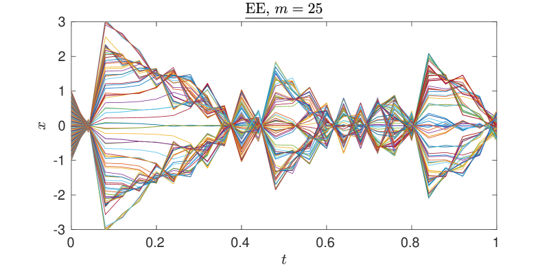
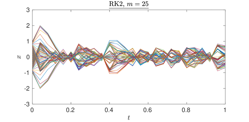
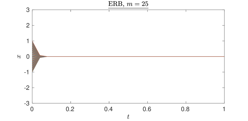
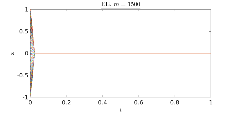
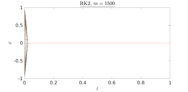
We finally notice that we can draw similar conclusions in a deterministic scenario, i.e., when . In fact, the randomness in the dynamics does not mitigate the need of a strong time step size restriction for the standard explicit integrators. We demonstrate this by performing a numerical experiment setting . For the time marching, we consider the classical first-order explicit Euler method and the second-order Runge–Kutta scheme
also known as Heun’s method or explicit trapezoidal rule. As exponential integrator, we employ the standard explicit Rosenbrock–Euler method (8), which is second-order accurate. We report in Figures 4 and 5 the results of the experiments. As expected, both explicit Euler and Heun’s method are not able to correctly capture the dynamics of the system, unless a consistently high number of time steps is employed. This is in contrast with what happens for the exponential Rosenbrock–Euler method, which already with time steps reaches the expected state in a stable way.
5.2 Tests with turnpike control
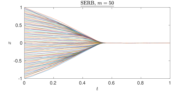
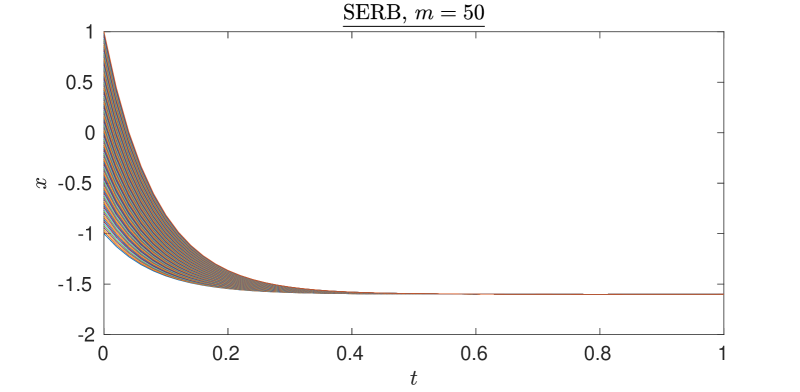
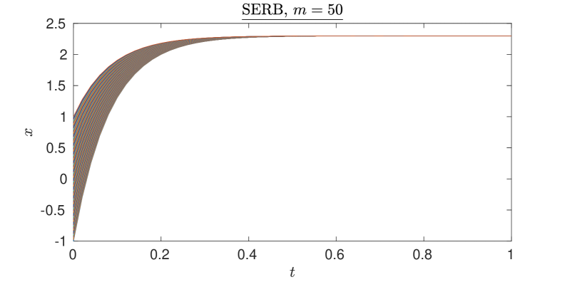
We now perform some numerical examples that show the validity and the effectiveness of the turnpike property in our setting. To this aim, we start by considering the interaction kernel (26), setting . We choose as decay parameter for the Lyapunov functional and impose the threshold value (see Section 4.4). Then, according to formula (25), once we set the target point we are able to find an estimate for the turnpike time . Remark that, in terms of actual simulation, we split the time interval into and . In we perform the cheap time integration of equation (19) by means of the exponential Rosenbrock–Euler method (see formula (20)) or the explicit Euler method, depending on the time marching framework we are considering. We stress that when cheap integrating with the exponential integrator, we could perform a single step to reach the time (in contrast to, e.g., the explicit Euler method). This is indeed the case since, at this stage, the equation is linear, and therefore the exponential integrator solves it exactly (as already discussed in the proof of Lemma 4.3). Nevertheless, just for visualization purposes, in the experiment we computed the position of the agents at each time discretization point. Finally, in the time interval the static control can be employed, which in our case is zero. Therefore, in we are essentially evolving the dynamics as if it was uncontrolled (as done in the experiments in the previous subsection). The number of time steps is always set to .
For the first experiment we choose as target state. The turnpike time, according to formula (25), is then selected as . The results are reported in Figure 6 (top and center plot). As expected, since there is no source of stiffness in the cheap integration part, the standard explicit method and the exponential integrator qualitatively behave similarly. However, when the turnpike time is surpassed, the system is left uncontrolled and the instability coming from the stiff kernel arises in the Euler–Maruyama method (as already observed in the previous subsection). This, in turn, does not happen when working in the exponential integrators framework, which allow to reach the target point in a stable way. We then conclude that the latter is clearly the preferred approach in this context.
We now test the validity of the exponential integration procedure also when the target point is outside the initial interval . In particular, we set and select accordingly the turnpike time as . The result, presented in Figure 6 (bottom plot) is in perfect agreement with what expected.
Finally, we employ the proposed approach in the context of a non-symmetric kernel. To this aim, we de-symmetrize (26) by considering instead
| (28) |
with
In fact, the agents are linearly weighted with magnitudes controlled by and . The parameters are set to , , and . The result of the experiment with target point and (obtained once again setting and ) is summarized in Figure 7. The outcome is in line with what expected, i.e., the employment of a non-symmetric kernel does not generate issues for the turnpike control and, in particular, does not nullify the convergence of the system to the desired state.
6 Conclusions
In this work, we established the turnpike property for discrete-time stochastic optimal control problems governing interacting agents. By leveraging strict dissipativity and cheap control conditions, we showed that the turnpike phenomenon persists despite the presence of noise. To address numerical challenges arising from stiffness, we employed exponential integrators, demonstrating their stability advantages over standard explicit schemes. Our numerical experiments confirmed that the proposed approach effectively maintains the desired asymptotic behavior in several scenarios. For future work, an interesting direction would be to extend the analysis beyond the mean value and investigate the variance of the stochastic dynamics. This would provide a deeper understanding of the fluctuations around the mean and their impact on the control strategy. Additionally, exploring more complex interaction kernels, including unbounded kernels, could lead to further insights into the turnpike behavior of large-scale agent systems.
Acknowledgments
The authors are deeply grateful to Prof. Michael Herty for its continuous interest in this work and for the numerous constructive discussions. The authors are members of the Gruppo Nazionale Calcolo Scientifico-Istituto Nazionale di Alta Matematica (GNCS-INdAM). F. Cassini holds a post-doc fellowship funded by INdAM. C. Segala thanks the Swiss National Science Foundation (SNSF) for the financial support through the grant number 215528, Large-scale kernel methods in financial economics.
References
- [1] Al-Mohy, A. H., and Higham, N. J. Computing the action of the matrix exponential, with an application to exponential integrators. SIAM J. Sci. Comput. 33, 2 (2011), 488–511.
- [2] Albi, G., Bicego, S., and Kalise, D. Gradient-augmented supervised learning of optimal feedback laws using state-dependent Riccati equations. IEEE Control Syst. Lett. 6 (2022), 836–841.
- [3] Albi, G., Caliari, M., Calzola, E., and Cassini, F. Exponential integrators for a mean-field selective optimal control problem. J. Approx. Softw. 1, 2 (2024).
- [4] Albi, G., Herty, M., Kalise, D., and Segala, C. Moment-driven predictive control of mean-field collective dynamics. SIAM J. Control Optim. 60, 2 (2022), 814–841.
- [5] Albi, G., Herty, M., and Segala, C. Robust feedback stabilization of interacting multi-agent systems under uncertainty. Applied Mathematics & Optimization 89, 1 (2024), 16.
- [6] Albi, G., and Pareschi, L. Selective model-predictive control for flocking systems. Commun. Appl. Ind. Math. 9, 2 (2018), 4–21.
- [7] Balagué, D., Carrillo, J., Laurent, T., and Raoul, G. Nonlocal interactions by repulsive–attractive potentials: Radial ins/stability. Phys. D: Nonlinear Phenom. 260 (2013), 5–25.
- [8] Bellomo, N., Degond, P., and Tadmor, E., Eds. Active particles. Vol. 1. Advances in theory, models, and applications. Modeling and Simulation in Science, Engineering and Technology. Birkhäuser/Springer, Cham, 2017.
- [9] Bellomo, N., Degond, P., and Tadmor, E., Eds. Active particles. Vol. 2. Advances in theory, models, and applications. Modeling and Simulation in Science, Engineering and Technology. Birkhäuser/Springer, Cham, 2019.
- [10] Caliari, M., and Cassini, F. Efficient simulation of complex Ginzburg–Landau equations using high-order exponential-type methods. Appl. Num. Math. 206 (2024), 340–357.
- [11] Caliari, M., and Cassini, F. A second order directional split exponential integrator for systems of advection–diffusion–reaction equations. J. Comput. Phys. 498 (2024), 112640.
- [12] Caliari, M., Cassini, F., Einkemmer, L., and Ostermann, A. Accelerating exponential integrators to efficiently solve semilinear advection-diffusion-reaction equations. SIAM J. Sci. Comput. 46, 2 (2024), A906–A928.
- [13] Caliari, M., Cassini, F., and Zivcovich, F. BAMPHI: Matrix-free and transpose-free action of linear combinations of -functions from exponential integrators. J. Comput. Appl. Math. 423 (2023), 114973.
- [14] Caliari, M., Einkemmer, L., Moriggl, A., and Ostermann, A. An accurate and time-parallel rational exponential integrator for hyperbolic and oscillatory PDEs. J. Comput. Phys. 437 (2021), 110289.
- [15] Caponigro, M., Fornasier, M., Piccoli, B., and Trélat, E. Sparse stabilization and optimal control of the cucker-smale model. Math. Control Relat. Fields 3 (2013), 447–466.
- [16] Cordier, S., Pareschi, L., and Toscani, G. On a kinetic model for a simple market economy. J. Stat. Phys. 120, 1-2 (jul 2005), 253–277.
- [17] Gaudreault, S., Rainwater, G., and Tokman, M. KIOPS: A fast adaptive Krylov subspace solver for exponential integrators. J. Comput. Phys. 372 (2018), 236–255.
- [18] Grüne, L. Dissipativity and optimal control: examining the turnpike phenomenon. IEEE Control Syst. 42, 2 (2022), 74–87.
- [19] Grun̈e, L., and Guglielmi, R. Turnpike properties and strict dissipativity for discrete time linear quadratic optimal control problems. SIAM J. Control Optim. 56, 2 (2018), 1282–1302.
- [20] Gugat, M., Herty, M., Liu, J., and Segala, C. The turnpike property for high-dimensional interacting agent systems in discrete time. Optim. Control Appl. Meth. 45, 6 (2024), 2557–2571.
- [21] Gugat, M., Herty, M., and Segala, C. The turnpike property for mean-field optimal control problems. Eur. J. Appl. Math. (2023), 1–15.
- [22] Herty, M., Pareschi, L., and Steffensen, S. Mean-field control and Riccati equations. Netw. Heterog. Media 10, 3 (2015), 699–715.
- [23] Herty, M., and Ringhofer, C. Averaged kinetic models for flows on unstructured networks. Kinet. Relat. Models 4 (12 2011).
- [24] Higham, D. J. An Algorithmic Introduction to Numerical Simulation of Stochastic Differential Equations. SIAM rev. 43, 3 (2001), 525–546.
- [25] Hochbruck, M., and Ostermann, A. Explicit Exponential Runge–Kutta Methods for Semilinear Parabolic Problems. SIAM J. Numer. Anal. 43, 3 (2005), 1069–1090.
- [26] Hochbruck, M., and Ostermann, A. Exponential integrators. Acta Numer. 19 (2010), 209–286.
- [27] Hochbruck, M., Ostermann, A., and Schweitzer, J. Exponential Rosenbrock-type Methods. SIAM J. Numer. Anal. 47, 1 (2009), 786–803.
- [28] Lord, G. J., and Tambue, A. Stochastic exponential integrators for the finite element discretization of SPDEs for multiplicative and additive noise. IMA J. Numer. Anal. 33 (2013), 515–543.
- [29] Lord, G. J., and Tambue, A. Stochastic exponential integrators for a finite element discretisation of SPDEs with additive noise. Appl. Num. Math. 136 (2019), 163–182.
- [30] Luan, V. T., Pudykiewicz, J. A., and Reynolds, D. R. Further development of efficient and accurate time integration schemes for meteorological models. J. Comput. Phys. 376 (2019), 817–837.
- [31] Ma, L., Wang, Z., Han, Q.-L., and Liu, Y. Consensus control of stochastic multi-agent systems: a survey. Science China Information Sciences 60 (2017), 1–15.
- [32] Mukam, J. D., and Tambue, A. Strong Convergence Analysis of the Stochastic Exponential Rosenbrock Scheme for the Finite Element Discretization of Semilinear SPDEs Driven by Multiplicative and Additive Noise. J. Sci. Comput. 74 (2018), 937–978.
- [33] Ou, R., Baumann, M. H., Grüne, L., and Faulwasser, T. A simulation study on turnpikes in stochastic lq optimal control. IFAC-PapersOnLine 54, 3 (2021), 516–521.
- [34] Schießl, J., Baumann, M. H., Faulwasser, T., and Grüne, L. On the relationship between stochastic turnpike and dissipativity notions. IEEE Transactions on Automatic Control (2024), 1–13.
- [35] Skaflestad, B., and Wright, W. M. The scaling and modified squaring method for matrix functions related to the exponential. Appl. Numer. Math. 59, 3–4 (2009), 783–799.
- [36] Willems, J. C. Dissipative dynamical systems part I: General theory. Arch. Ratio. Mech. Anal. 45, 5 (1972), 321–351.
- [37] Zaslavski, A. J. Turnpike Properties in the Calculus of Variations and Optimal Control, 1st ed., vol. 80 of Nonconvex Optimization and Its Applications. Springer US, New York, NY, 2006.
- [38] Zaslavski, A. J. Necessary and sufficient turnpike conditions. Pure Appl. Funct. Anal. 4, 2 (2019), 463–476.