The Value of Goal Commitment in Planning

Abstract

In this paper, we revisit the concept of goal commitment from early planners in the presence of current forward chaining heuristic planners. We present a compilation that extends the original planning task with commit actions that enforce the persistence of specific goals once achieved, thereby committing to them in the search sub-tree. This approach imposes a specific goal achievement order in parts of the search tree, potentially introducing dead-end states. This can reduce search effort if the goal achievement order is correct. Otherwise, the search algorithm can expand nodes in the open list where goals do not persist. Experimental results demonstrate that the reformulated tasks suit state-of-the-art agile planners, enabling them to find better solutions faster in many domains.

Introduction

Automated Planning deals with the task of finding a sequence of actions, namely a plan, which achieves a goal from a given initial state (Ghallab, Nau, and Traverso 2004). Early planners approached this task from two different perspectives: partial-order and total-order planning. Partial-order planners (Barrett and Weld 1994) searched in the space of plans and followed a least commitment strategy, where the actions in the plan were only partially ordered. On the other hand, total-order planners (Veloso et al. 1995) kept a state of the world, and usually committed to a particular goal ordering while planning. Both approaches were outperformed by heuristic search planners (Bonet and Geffner 2001), where there is no explicit goal commitment decision.

In this paper we revisit the concept of goal commitment from early planners in the presence of current forward chaining heuristic planners. We present a compilation that extends the original planning task with $\mathsf{commit}$ actions that allow the planner to enforce the persistence of specific goals once they are achieved, effectively committing to them in the search sub-tree. By doing so, our compilation imposes a specific goal achievement ordering in parts of the search tree. This commitment might introduce dead-end states in cases where committing to the goal is not the right choice, as it needs to be temporary undone to solve the task. This can help on reducing the search effort if the commitment on that goal achievement ordering is correct. When it is not, the search algorithm can always resort to expanding those nodes in the open list where goals do not persist. Figure 1 shows an excerpt of the search tree in a compiled blocks task. $I$ represents the initial state and $G$ the goal. Green blocks depict persistent goals, i.e., blocks that cannot be unstacked once they are stacked. The left part of the tree is new compared to the search tree of the original task, and contains states with persistent goals. By creating this new sub-tree, we are allowing heuristic search planners to realize that committing to some goals might be beneficial, potentially reducing the number of expanded and generated states, and guiding the search faster towards good solutions.

We evaluate the performance of lamaF (Richter and Westphal 2010), a state-of-the-art agile planner, when solving both the original and the reformulated task with $\mathsf{commit}$ actions. Experimental results show that the reformulated tasks are amenable for lamaF, being able to find better solutions faster in many domains.

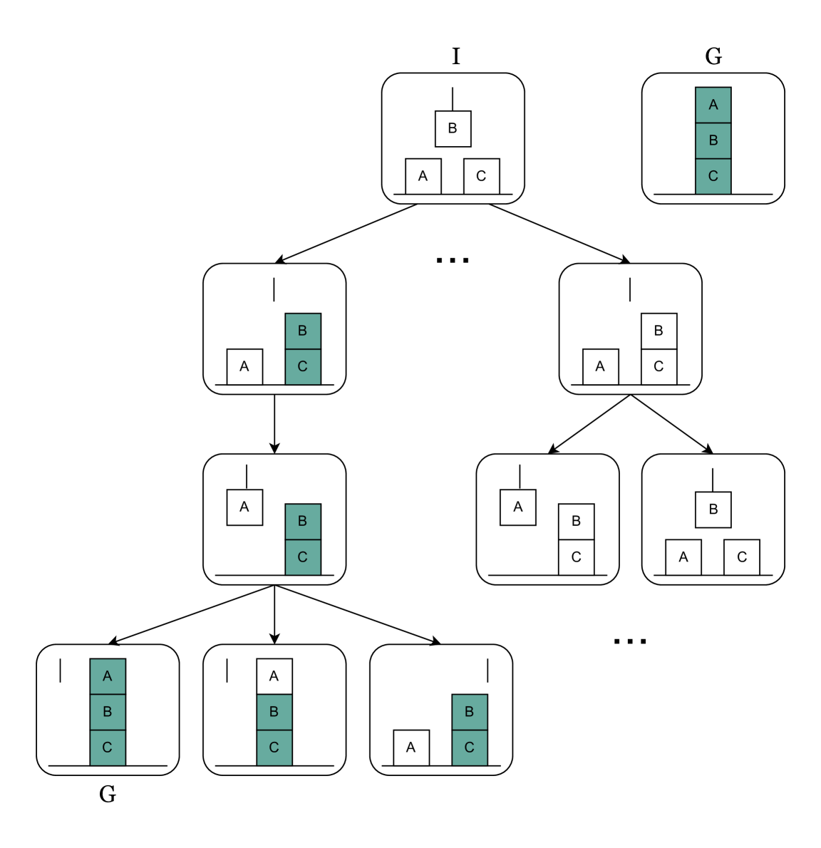
Figure 1: Compiled task in a blocks instance. Green blocks depict persistent goals, i.e., blocks that cannot be unstacked.

Background

We formally define a planning task as follows:

Definition 1.

A strips planning task is a tuple ${\cal P}=\langle F,A,I,G\rangle$, where $F$ is a set of fluents, $A$ is a set of actions, $I\subseteq F$ is an initial state, and $G\subseteq F$ is a goal specification.

A state $s\subseteq F$ is a set of fluents that are true at a given time. A state $s\subseteq F$ is a goal state iff $G\subseteq s$. Each action $a\in A$ is described by its name $\textsc{name}(a)$, a set of positive and negative preconditions $\textsc{pre}^{+}(a)$ and $\textsc{pre}^{-}(a)$, add effects $\textsc{add}(a)$, delete effects $\textsc{del}(a)$, and cost $c(a)$. An action $a$ is applicable in a state $s$ iff $\textsc{pre}^{+}(a)\subseteq~s$ and $\textsc{pre}^{-}(a)\cap s=\emptyset$. We define the result of applying an action in a state as $\gamma(s,a)=(s\setminus\textsc{del}(a))\cup\textsc{add}(a)$. A sequence of actions $\pi=(a_{1},\ldots,a_{n})$ is applicable in a state $s_{0}$ if there are states $(s_{1}.\ldots,s_{n})$ such that $a_{i}$ is applicable in $s_{i-1}$ and $s_{i}=\gamma(s_{i-1},a_{i})$. The resulting state after applying a sequence of actions is $\Gamma(s,\pi)=s_{n}$, and $c(\pi)=\sum_{i}^{n}c(a_{i})$ denotes the cost of $\pi$. A state $s$ is reachable from state $s^{\prime}$ iff there exists an applicable action sequence $\pi$ such that $s\subseteq\Gamma(s^{\prime},\pi)$. A state $s$ is a dead-end state iff it is not a goal state and no goal state is reachable from $s$. The solution to a planning task ${\cal P}$ is a plan, i.e., a sequence of actions $\pi$ such that $G\subseteq\Gamma(I,\pi)$. A plan with minimal cost is optimal.

Planning with Commit Actions

The aim of our compilation is to extend the original planning task with $\mathsf{commit}$ actions that allow the planner to enforce the persistence of specific goals once they are achieved. In particular, we will only focus on committing to those goals that are not already true in the initial state, and that can be achieved through actions in $A$. Formally:

$$\bar{G}=\{g_{i}\in G\setminus I\mid\exists a\in A,g_{i}\in\textsc{add}(a)\}\}$$

To ensure that goals in $\bar{G}$ remain achieved throughout the planning process, we extend the original set of propositions $F$ with a new set of $\mathsf{commit}$ propositions that we denote $F_{c}$. Each goal $g_{i}\in\bar{G}$ is associated with a $\mathsf{commit}$ version, which tracks whether $g_{i}$ has been achieved and should remain true. Formally, we define $F_{c}=\bigcup_{g_{i}\in\bar{G}}\{g_{i}\mbox{-}\mathsf{commit}\}$.

We also update the set of original actions $A$ to account for three distinct groups based on their interaction with the goals. We define: (i) $A^{G}$ as the set of actions that add goals: $A^{G}=\{a\in A\mid\bar{G}\cap\textsc{add}(a)\not=\emptyset\}$, (ii) $A^{\neg G}$ as the actions that remove goals: $A^{\neg G}=\{a\in A\mid\bar{G}\cap\textsc{del}(a)\not=\emptyset\}$, and (iii) $A^{L}$ as the actions that neither add nor delete goals: $A^{L}=\{a\in A\mid\bar{G}\cap\textsc{add}(a)=\emptyset\land\bar{G}\cap\textsc{del}(a)=\emptyset\}$.

The first type of actions, $A^{G}$, corresponds to the subset of actions that make goals in $\bar{G}$ true. Given that our compilation persists certain goals, we need to include a set of $\mathsf{commit}$ actions specifically aimed at achieving the $g_{i}\mbox{-}\mathsf{commit}$ goals. Since in general some actions can achieve multiple goal propositions, for each action $a^{G}\in A^{G}$, we first define $C_{a^{G}}$ to be a set containing all the possible combinations of $\mathsf{commit}$ goals in $\textsc{add}(a^{G})\cap\bar{G}$. This set will have $2^{n}-1$ subsets, where $n$ is the number of goals in $\textsc{add}(a^{G})\cap\bar{G}$. For example, assuming $\textsc{add}(a^{G})\cap\bar{G}=\{x,y\}$, $C_{a^{G}}=\{\{x\},\{y\},\{x,y\}\}$. Then, we introduce a new set of $\mathsf{commit}$ actions $A^{\mathsf{C}}$ as follows: for every action $a^{G}\in A^{G}$, we keep the original action in $A^{\mathsf{C}}$, and we also introduce $|C_{a^{G}}|$ new actions. Each $\mathsf{commit}$ action $a^{\mathsf{C}}_{i}\in A^{\mathsf{C}}$, with $i\in C_{a^{G}}$, is defined as follows:

• $\textsc{name}(a^{\mathsf{C}}_{i})=\textsc{name}(a^{G})\mbox{-}\mathsf{commit}\mbox{-}i$

• $\textsc{pre}^{+}(a^{\mathsf{C}}_{i})=\textsc{pre}^{+}(a^{G})$, $\textsc{pre}^{-}(a^{\mathsf{C}}_{i})=\textsc{pre}^{-}(a^{G})$

• $\textsc{del}(a^{\mathsf{C}}_{i})=\textsc{del}(a^{G})$

• $\textsc{add}(a^{\mathsf{C}}_{i})=\textsc{add}(a^{G})\cup\{\cup_{j\in i}g_{j}\mbox{-}\mathsf{commit}\}$

The second type of actions, $A^{\neg G}$, corresponds to the subset of actions that delete goals in $\bar{G}$. In this case, we need to ensure that these actions do not delete a goal that is already $\mathsf{commit}$. This requires checking the preconditions to avoid interfering with goals that must be maintained. As we did for the first type of actions, for every $a^{\neg G}\in A^{\neg G}$, we define $C_{a^{\neg G}}$ as the set of all the possible combinations of goals in $\textsc{del}(a^{\neg G})\cap\bar{G}$. Then, we introduce a new set of actions $A^{\neg\mathsf{C}}$ composed as follows: for every action $a^{\neg G}\in A^{\neg G}$, we introduce $|C_{a^{\neg G}}|$ actions. Each $\mathsf{forcecommit}$ action $a^{\neg\mathsf{C}}_{i}\in A^{\neg\mathsf{C}}$, with $i\in C_{a^{\neg G}}$, is defined as follows:

• $\textsc{name}(a^{\neg\mathsf{C}}_{i})=\textsc{name}(a^{\neg G})\mbox{-}\mathsf{forcecommit}\mbox{-}i$

• $\textsc{pre}^{+}(a^{\neg\mathsf{C}}_{i})=\textsc{pre}(a^{\neg G})$

• $\textsc{pre}^{-}(a^{\neg\mathsf{C}}_{i})=\textsc{pre}(a^{\neg G})\cup\{\cup_{j\in i}g_{j}\mbox{-}\mathsf{commit}\}$

• $\textsc{del}(a^{\neg\mathsf{C}}_{i})=\textsc{del}(a^{\neg G})$, $\textsc{add}(a^{\neg\mathsf{C}}_{i})=\textsc{add}(a^{\neg G})$

The third type of actions, $A^{L}$, includes those that do not interact with the goals in $\bar{G}$ - that is, they neither remove nor add goals. We keep the actions $a\in A^{L}$ unchanged.

The new planning task is defined as follows:

Definition 2.

Given a planning task ${\cal P}=\langle F,A,I,G\rangle$, a commit planning task is defined as a tuple ${\cal P}_{\mathsf{c}}=\langle F^{\prime},A^{\prime},I,G^{\prime}\rangle$ where,

• $F^{\prime}=F\cup F_{c}$

• $A^{\prime}=A^{\mathsf{C}}\cup A^{\neg\mathsf{C}}\cup A^{L}$

• $G^{\prime}=\{G\setminus\bar{G}\}\cup_{g_{i}\in\bar{G}}\{g_{i}\mbox{-}\mathsf{commit}\}$

Theorem 1.

If ${\cal P}$ is solvable, ${\cal P}_{\mathsf{c}}$ is also solvable.

Proof.

Let $\pi$ be a solution for ${\cal P}$. We need to show that there exists a plan $\pi^{\prime}$ that solves ${\cal P}_{\mathsf{c}}$ comprised by the same sequence of actions as $\pi$, only varying their version, i.e. we include actions that allow us to have $\mathsf{commit}$ and $\mathsf{forcecommit}$ versions. For each action $a\in\pi$, there could be these cases:

Case 1. $a\in A^{L}$, then $\pi^{\prime}$ will use $a$.

Case 2. $a\in A^{\neg G}$ is replaced by its corresponding $\mathsf{forcecommit}$ action $a^{\prime}\in A^{\neg\mathsf{C}}$. They differ only in their preconditions related to $\mathsf{commit}$ goals. If such action appears in $\pi$, it means there will be another action $a^{\prime\prime}\in\pi$ that will achieve the goal that is being temporary deleted.

Case 3. $a\in A^{G}$. We differentiate two sub-cases: (i) when $a$ is not the last action in the plan achieving the goals in $\textsc{add}(a)\cap\bar{G}$, this action is replaced by the original action that we keep in $A^{\mathsf{C}}$; and (ii) when $a$ is the last action in the plan achieving the goals in $\textsc{add}(a)\cap\bar{G}$, this action is replaced by its corresponding $a^{\mathsf{C}}_{i}\in A^{\mathsf{C}}$ where $i\in C_{a^{G}}$.

For every $g_{i}\in G$, we have that either $g_{i}\in G^{\prime}$, and it is correctly achieved by the same actions present in $A^{\prime}$, or $g_{i}\in\bar{G}$ and corresponds to a $\mathsf{commit}$ version $g_{i}\mbox{-}\mathsf{commit}\in G^{\prime}$ and it is correctly achieved by $\mathsf{commit}$ actions in $A^{\mathsf{C}}$. ∎

Theorem 2.

Any plan $\pi^{\prime}$ that solves ${\cal P}_{\mathsf{c}}$ is a plan for the original problem ${\cal P}$.

Proof.

Let $\pi^{\prime}$ be a solution for ${\cal P}_{\mathsf{c}}$. We need to show that there is a plan $\pi$ that can be mapped from $\pi^{\prime}$ which is a solution for ${\cal P}$. Each action in $\pi^{\prime}$ falls into one of three cases: (i) $a\in A^{L}$: we leave them as is in $\pi$; (ii) $a\in A^{\mathsf{C}}$: they are substituted in $\pi$ by their counterparts in $A^{G}$; (iii) $a\in A^{\neg\mathsf{C}}$: they are substituted in $\pi$ by their counterparts in $A^{\neg G}$, which are equivalent to the original actions in ${\cal P}$, regarding their effects. Their preconditions in ${\cal P}_{\mathsf{c}}$ include $\mathsf{commit}$ attributes, but this only restricts action applicability in ${\cal P}_{\mathsf{c}}$, not in ${\cal P}$. Lastly, for all $g_{i}^{\prime}\in G^{\prime}$, we have that either $g_{i}^{\prime}\in G$ or $g_{i}^{\prime}$ is the $\mathsf{commit}$ version of a $g_{i}\in G$. Then $G$ is correctly achieved in ${\cal P}$. ∎

Evaluation

	Coverage		SAT Score		AGL Score
Domain (#Problems)	${\cal P}$	${\cal P}_{\mathsf{c}}$	${\cal P}$	${\cal P}_{\mathsf{c}}$	${\cal P}$	${\cal P}_{\mathsf{c}}$
agricola18 (20)	12	9	12.0	9.0	4.1	3.5
airport (50)	34	34	34.0	33.9	33.1	33.0
barman11 (20)	20	20	18.7	19.9	18.4	18.9
barman14 (20)	20	20	17.8	19.8	15.9	17.7
blocks (35)	35	35	22.7	35.0	56.3	56.4
childsnack14 (20)	6	6	6.0	6.0	7.1	7.1
data-network18 (20)	12	12	12.0	11.9	9.3	8.6
depot (22)	20	21	18.8	20.1	21.5	22.6
driverlog (20)	20	20	17.7	19.3	26.7	30.7
elevators08 (30)	30	30	28.5	28.7	36.5	36.4
elevators11 (20)	20	20	19.1	18.8	14.1	14.2
floortile11 (20)	6	6	5.7	5.8	2.1	2.3
floortile14 (20)	2	2	1.9	1.9	1.5	1.4
freecell (80)	77	80	75.1	75.8	80.6	83.0
ged14 (20)	20	0	20	0	20.0	0
grid (5)	5	5	4.9	5.0	6.5	6.5
gripper (20)	20	20	20.0	20.0	32.8	32.2
hiking14 (20)	20	20	20.0	19.9	17.5	17.5
logistics00 (28)	28	28	27.6	27.7	46.3	46.1
logistics98 (35)	35	34	34.9	33.7	40.9	40.8
miconic (150)	150	150	150.0	150.0	230.7	230.7
movie (30)	30	30	26.2	30.0	54.4	54.2
mprime (35)	35	35	35.0	35.0	46.8	46.8
mystery (30)	19	19	18.9	19.0	25.6	25.5
nomystery11 (20)	12	12	12.0	12.0	15.7	15.6
openstacks08 (30)	30	30	21.5	30.0	39.7	37.2
openstacks11 (20)	20	20	16.6	20.0	15.5	13.3
openstacks14 (20)	20	20	18.0	20.0	9.0	6.8
openstacks (30)	30	30	29.6	30.0	35.7	34.6
org-syn18 (20)	3	1	3.0	1.0	2.0	0.9
org-syn-split18 (20)	12	9	12.0	9.0	7.6	5.9
parcprinter-08 (30)	30	23	28.4	23.0	46.8	30.8
parcprinter11 (20)	20	10	19.0	10.0	27.7	9.7
parking11 (20)	20	5	19.9	4.4	13.6	1.6
parking14 (20)	20	2	20.0	1.9	8.7	0.6
pathways (30)	23	23	23.0	23.0	32.3	32.3
pegsol-08 (30)	30	30	22.4	29.8	43.4	39.1
pegsol11 (20)	20	20	15.0	19.9	26.8	24.3
pipes-notankage (50)	43	43	32.1	41.1	47.9	55.0
pipes-tankage (50)	43	37	35.5	36.3	41.7	39.0
psr-small (50)	50	50	50.0	47.5	87.0	85.8
quant-layout23 (20)	19	19	19.0	19.0	21.7	21.7
rovers (40)	40	40	40.0	40.0	54.1	54.1
satellite (36)	36	36	33.4	35.9	41.4	42.5
scanalyzer-08 (30)	30	30	27.0	28.0	36.6	34.9
scanalyzer11 (20)	20	20	17.6	18.9	21.3	20.6
snake18 (20)	4	4	4.0	4.0	2.6	2.5
sokoban08 (30)	29	28	25.8	27.2	26.3	24.8
sokoban11 (20)	19	18	16.5	17.4	13.9	12.8
spider18 (20)	16	14	15.8	12.6	6.7	5.9
storage (30)	19	21	16.9	19.9	26.6	28.0
tetris14 (20)	11	18	7.6	18.0	2.8	10.7
thoughtful14 (20)	15	16	14.9	16.0	15.7	15.9
tidybot11 (20)	16	16	16.0	16.0	10.8	10.8
tpp (30)	30	30	30.0	30.0	38.5	38.1
transport08 (30)	30	30	29.6	29.3	33.5	33.9
transport11 (20)	17	19	16.5	18.7	9.7	10.7
transport14 (20)	15	16	14.7	15.4	5.0	5.7
trucks (30)	15	15	15.0	15.0	16.2	16.1
visitall11 (20)	20	20	20.0	16.8	15.7	14.4
visitall14 (20)	20	20	20.0	17.0	8.1	7.2
woodworking08 (30)	30	30	29.7	28.1	30.4	30.8
woodworking11 (20)	20	20	19.5	19.2	14.5	14.3
zenotravel (20)	20	20	19.9	19.3	29.5	29.5
Total (1816)	1593	1521	1494.9	1486.8	1831.4	1754.5

Table 1: lamaF Coverage, SAT and AGL scores when solving the original (${\cal P}$) and compiled (${\cal P}_{\mathsf{c}}$) tasks. Bold figures indicate best performance.

Experimental Setting.

We selected all the strips tasks from the satisficing suite of the Fast Downward (Helmert 2006) benchmark collection. This gives us $1816$ tasks divided across $64$ domains. We reformulated each task using our approach and solved both the original (${\cal P}$) and the compiled (${\cal P}_{\mathsf{c}}$) tasks using lamaF, which is a state-of-the-art planner that won the agile track of the last International Planning Competition (IPC). lamaF runs the first iteration of the well-known lama planner (Richter and Westphal 2010), aiming to find a solution as soon as possible, disregarding its quality. It combines, among others: deferred heuristic evaluation, preferred operators, and multiple open lists guided by the ff (Hoffmann and Nebel 2001) and landmark-sum (Hoffmann, Porteous, and Sebastia 2004) heuristics. We run lamaF with a 8GB memory bound and a time limit of $900$s on Intel Xeon E5-2666 v3 CPUs @ 2.90GHz. We will report the following metrics:

Coverage: number of problems solved by lamaF.

SAT Score: $C^{*}/C$, where $C^{*}$ is the lowest cost found among both tasks, and $C$ is the plan’s cost lamaF gets in the the given task. Higher numbers indicate better performance.

AGL Score: $1-log(T)/log(900)$, where $T$ lamaF runtime, which includes both the grounding and search time. Higher numbers indicate better performance.

AGL Score Improvement: $\frac{\mbox{Search time in }{\cal P}_{\mathsf{c}}}{\mbox{Search time in }{\cal P}}$. Values above $1$ indicate that lamaF solves ${\cal P}_{\mathsf{c}}$ faster. Values below $1$ indicate that lamaF solves the original task faster.

Commit Expanded Ratio: ratio between the number of times lamaF expands a node through a $\mathsf{commit}$ action, and the number of $\mathsf{commit}$ actions in the returned plan. Higher numbers indicate the planner unsuccessfully tried more $\mathsf{commit}$ actions during search.

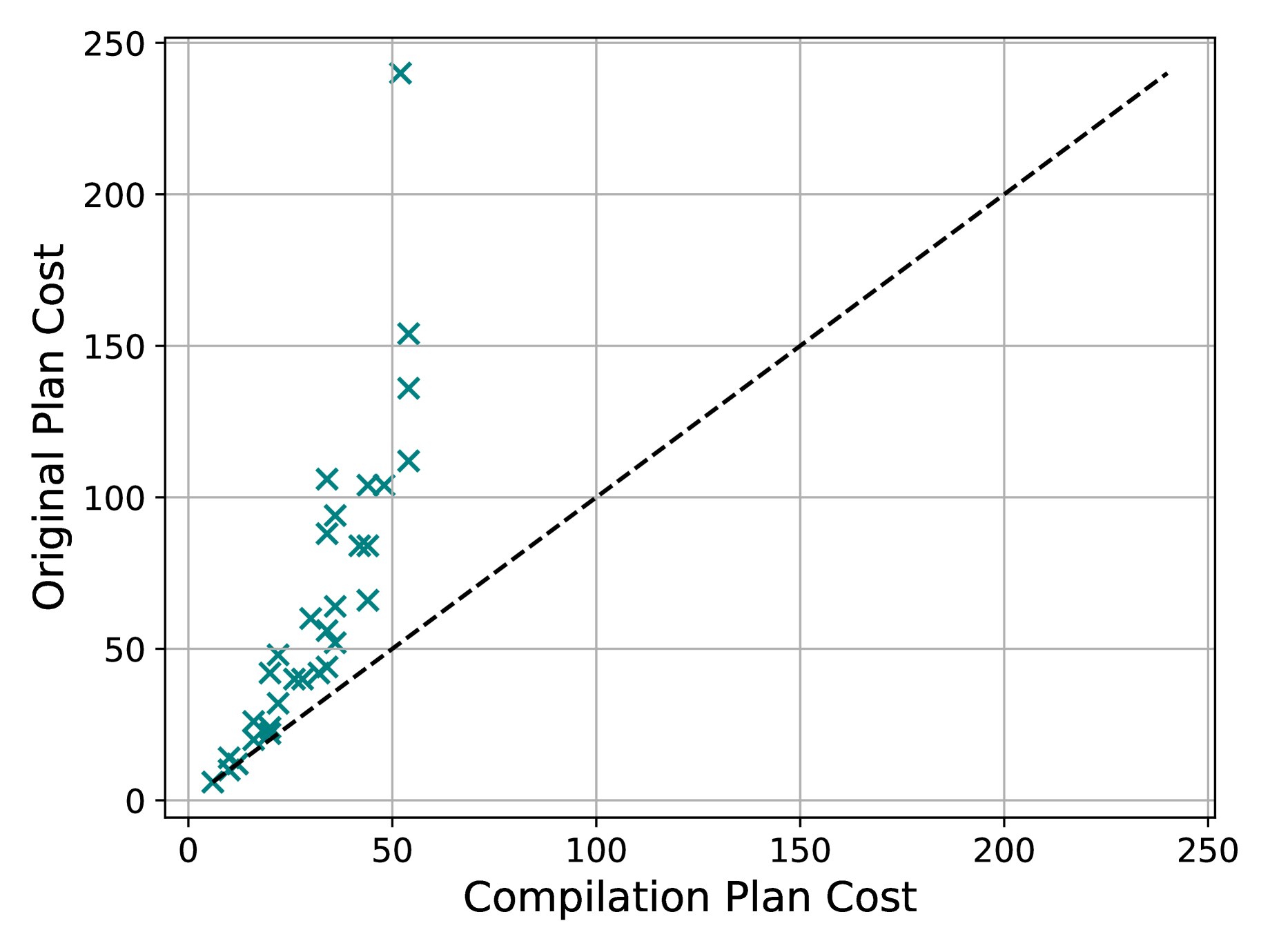
(a) blocks

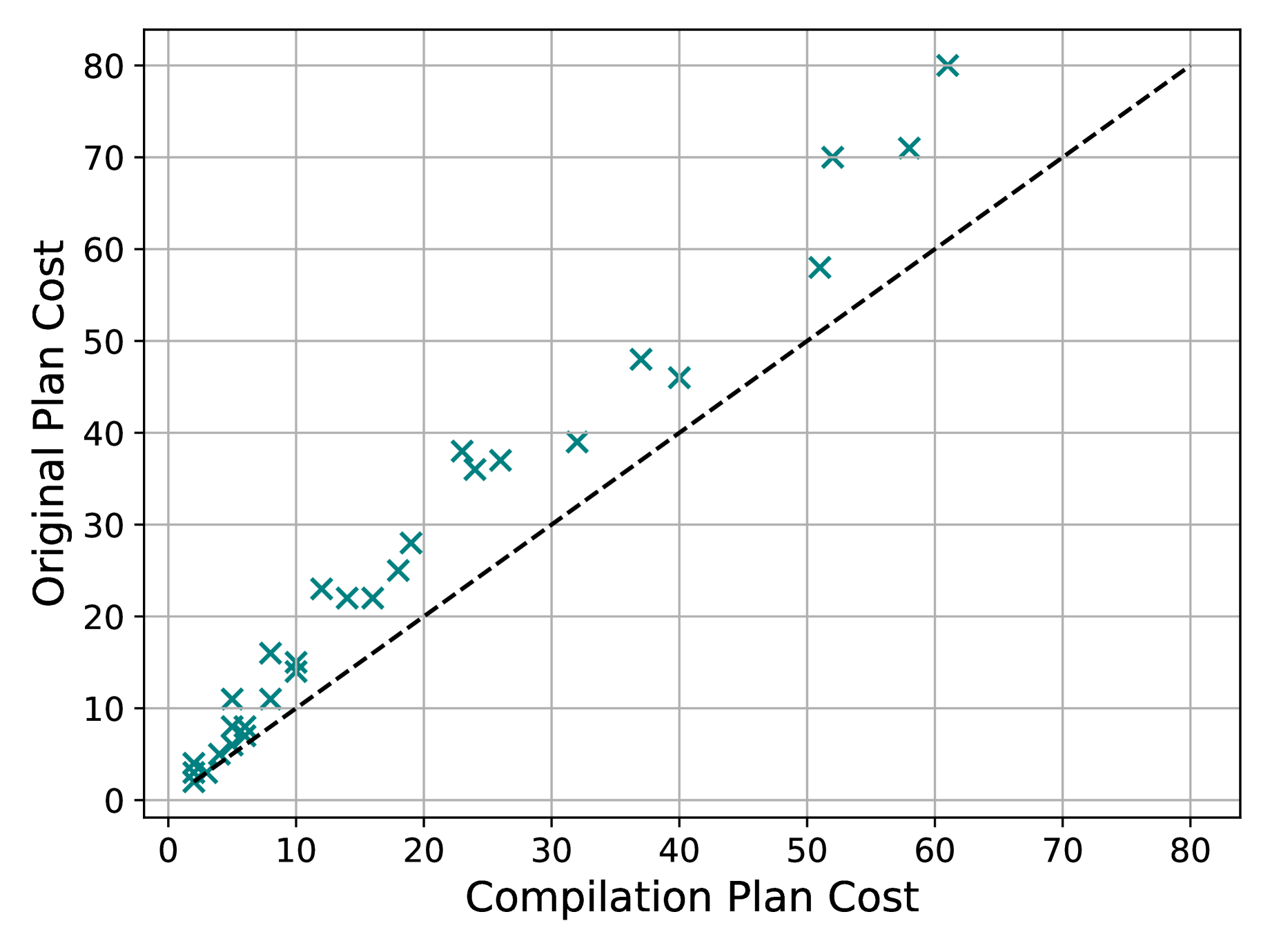
(b) openstacks08

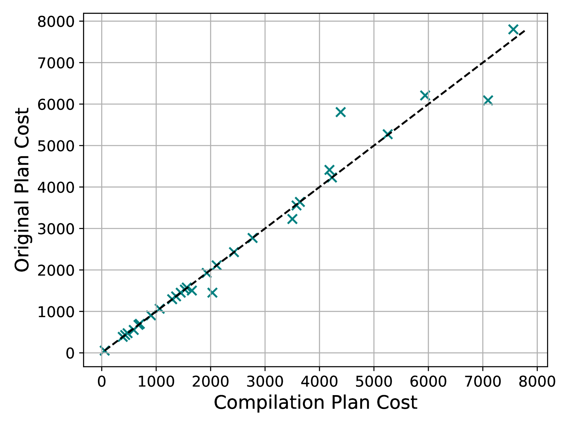
(c) transport08

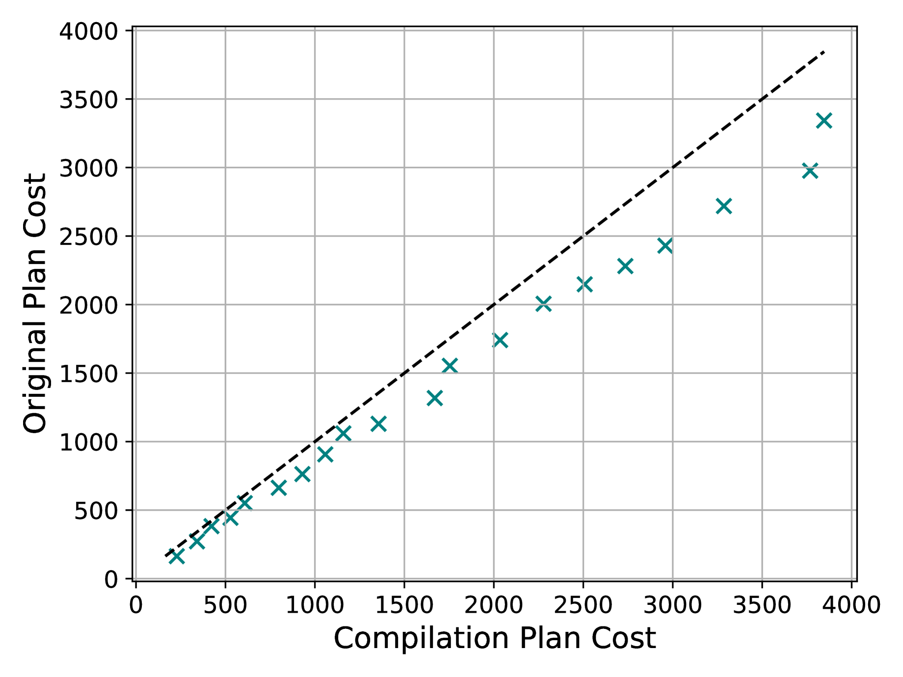
(d) visitall11

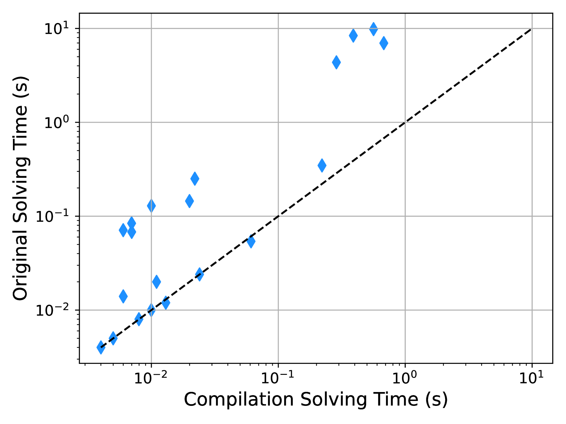
(e) driverlog

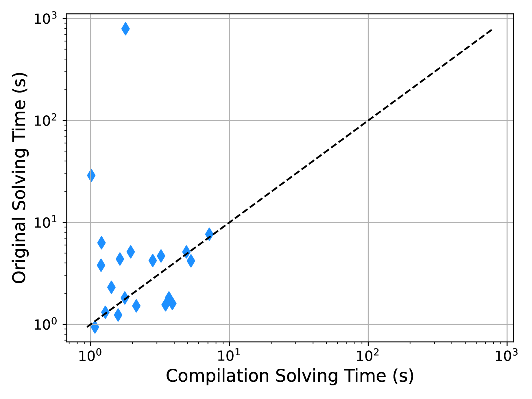
(f) barman14

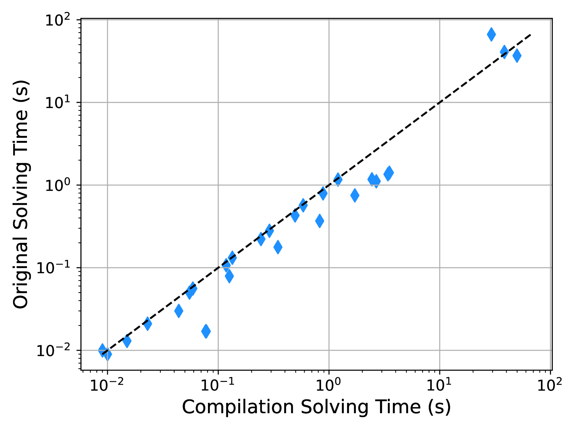
(g) scanalyzer08

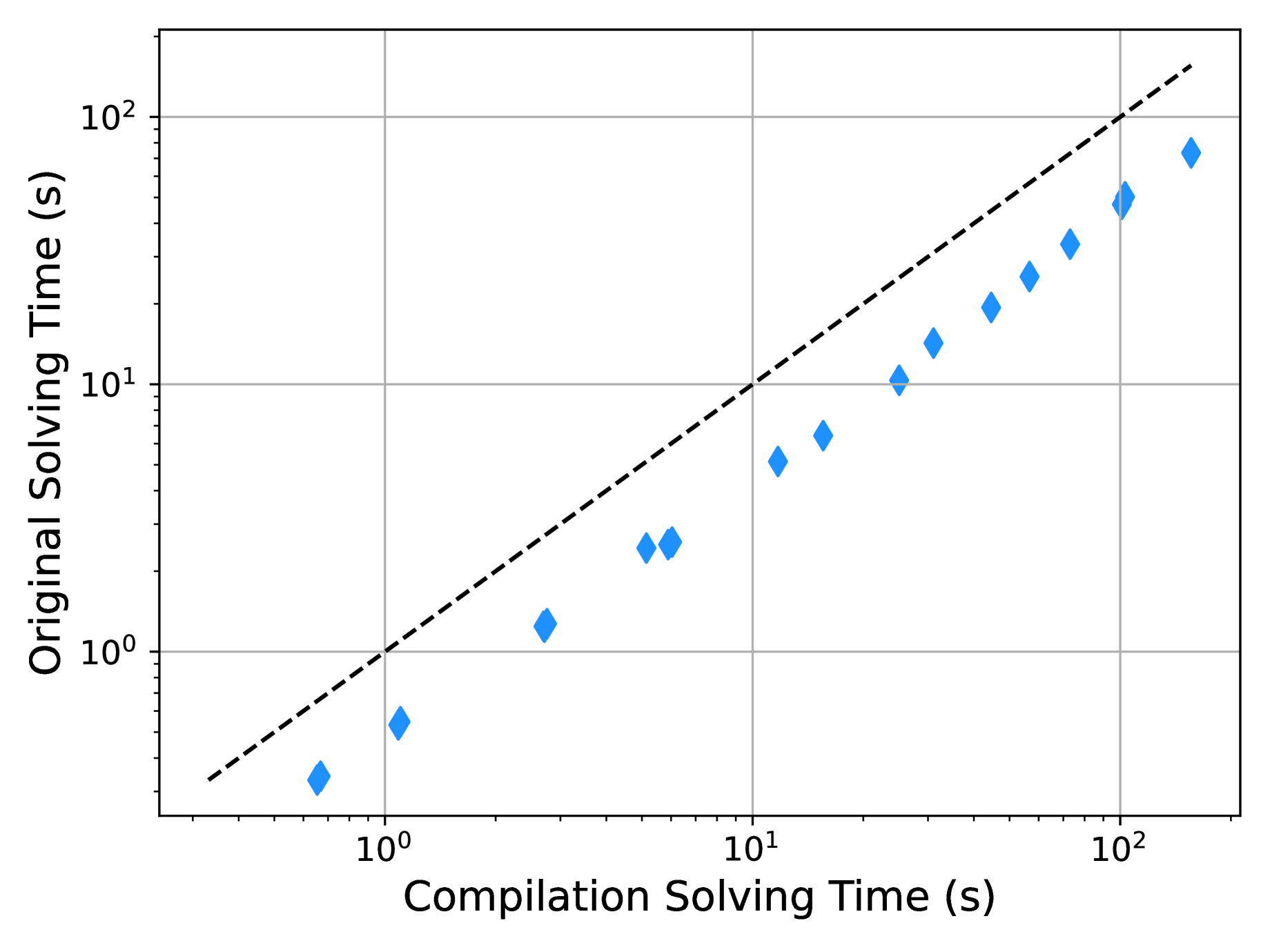
(h) openstacks11

Figure 2: lamaF plan cost (first row) and runtime (second row) when solving the original and compiled tasks in different domains. Points above the diagonal indicate better performance when solving the compiled task.

Results.

Table 1 shows the Coverage, SAT and AGL scores when solving the original (${\cal P}$) and the compiled (${\cal P}_{\mathsf{c}}$) tasks. Bold figures indicate best performance. As we can see, lamaF obtains better overall results when solving ${\cal P}$, getting slightly higher scores across all metrics compared to solving ${\cal P}_{\mathsf{c}}$. However, this performance difference greatly depends on the domain. Focusing on Coverage, lamaF solves more tasks in $7$ domains, the same in $44$ and less in $13$, when solving ${\cal P}_{\mathsf{c}}$ compared to ${\cal P}$. In some domains like ged14, lamaF can solve all the original tasks but none of the reformulated ones, highlighting that in some problems the planner might focus on trying $\mathsf{commit}$ actions that then needs to discard due to goals’ interactions. In others like tetris14, the reformulated task is more amenable for lamaF, being able to solve $7$ more problems. Focusing on the SAT score, solving ${\cal P}_{\mathsf{c}}$ yields higher scores in $30$ domains, the same in $13$ and lower in $21$. In most domains where lamaF can solve all the original and reformulated tasks, solving ${\cal P}_{\mathsf{c}}$ yields lower cost plans. This is the case of blocks, where solving the compiled task can give plans with up to $5$ times lower cost. The first row of Figure 2 shows the plan cost obtained by lamaF when solving both tasks across different domains. We report domains like blocks and openstacks, where solving ${\cal P}_{\mathsf{c}}$ is consistently better; domains like transport, where the results are problem dependent; and domains like visitall where the plans obtained when solving ${\cal P}_{\mathsf{c}}$ are consistently worse. Similar conclusions can be drawn if we focus on the AGL score. The second row of Figure 2 shows lamaF runtime in the original and reformulated task across different domains. Again, the results vary per domain, with some like driverlog where there is a clear benefit of using the compilation, and others like openstacks where getting better plans comes at the cost of slightly higher solving times.

Finally, we aimed to analyze how the advantage of solving the reformulated task depends on the planner’s ability to use $\mathsf{commit}$ actions to achieve goals that do not require reversal to solve the task. Figure 3 shows the results of this analysis. As we can see, there is a slight trend where most of the tasks with AGL Score Improvement $>1$ are those with lower Commit Expanded Ratio values. In particular, when Commit Expanded Ratio $<10$, i.e., the planner does not need to backtrack over many $\mathsf{commit}$ actions, we have $163$ problems with AGL Score Improvement $>1$ and $149$ where AGL Score Improvement $\leq 1$. On the other hand, when Commit Expanded Ratio $\geq 10$, i.e., the planner expands more $\mathsf{commit}$ actions that need to be later reverted due to goal interactions, we have only $66$ problems where solving the compiled task is faster vs $1438$ where it is slower.

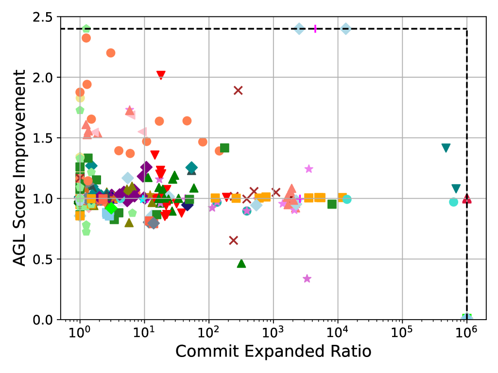
Figure 3: Colors and markers indicate different domains. Points at the $x=10^{6}$ line denote lamaF could not solve the compiled task. Points at the $y=2.5$ line denote lamaF could solve the compiled but not the original task.

Conclusions and Future Work

In this paper we have introduced a compilation that extends the original planning task with $\mathsf{commit}$ actions that allows planners to enforce the persistence of specific goals once they are achieved, effectively committing to them in the search sub-tree. Experimental results indicate that current heuristic search planners can successfully exploit this new task structure to generate better solutions faster in many domains. In future work we aim to explore how the reformulated tasks affect the performance of other planners. Given that planners typically combine (among others) search algorithms and heuristics, we would also like to identify the specific combinations that benefit from this compilation.

Disclaimer

This paper was prepared for informational purposes by the Artificial Intelligence Research group of JPMorgan Chase & Co. and its affiliates (”JP Morgan”) and is not a product of the Research Department of JP Morgan. JP Morgan makes no representation and warranty whatsoever and disclaims all liability, for the completeness, accuracy or reliability of the information contained herein. This document is not intended as investment research or investment advice, or a recommendation, offer or solicitation for the purchase or sale of any security, financial instrument, financial product or service, or to be used in any way for evaluating the merits of participating in any transaction, and shall not constitute a solicitation under any jurisdiction or to any person, if such solicitation under such jurisdiction or to such person would be unlawful.

References

- Barrett and Weld (1994) Barrett, A.; and Weld, D. S. 1994. Partial-order planning: Evaluating possible efficiency gains. Artificial Intelligence, 67(1): 71–112.
- Bonet and Geffner (2001) Bonet, B.; and Geffner, H. 2001. Planning as heuristic search. Artif. Intell., 129(1-2): 5–33.
- Ghallab, Nau, and Traverso (2004) Ghallab, M.; Nau, D. S.; and Traverso, P. 2004. Automated planning - theory and practice. Elsevier. ISBN 978-1-55860-856-6.
- Helmert (2006) Helmert, M. 2006. The fast downward planning system. Journal of Artificial Intelligence Research, 26: 191–246.
- Hoffmann and Nebel (2001) Hoffmann, J.; and Nebel, B. 2001. The FF planning system: Fast plan generation through heuristic search. Journal of Artificial Intelligence Research, 14: 253–302.
- Hoffmann, Porteous, and Sebastia (2004) Hoffmann, J.; Porteous, J.; and Sebastia, L. 2004. Ordered landmarks in planning. Journal of Artificial Intelligence Research, 22: 215–278.
- Richter and Westphal (2010) Richter, S.; and Westphal, M. 2010. The LAMA planner: Guiding cost-based anytime planning with landmarks. Journal of Artificial Intelligence Research, 39: 127–177.
- Veloso et al. (1995) Veloso, M.; Carbonell, J.; Perez, A.; Borrajo, D.; Fink, E.; and Blythe, J. 1995. Integrating planning and learning: The PRODIGY architecture. Journal of Experimental & Theoretical Artificial Intelligence, 7(1): 81–120.