Spectral properties of disordered insulating lattice under nonlinear electric field

Abstract

Quenched disorder in a solid state system can result in Anderson localization where electrons are exponentially localized and the system behaves like an insulator. In this study, we investigate the effect of a DC electric field on Anderson localization. The study highlights the case of a one-dimensional insulator chain with on-site disorder when a DC electric field is applied throughout the chain. We study spectral properties of an Anderson localized system in equilibrium and out-of-equilibrium using a full lattice nonequilibrium Green’s function method in the steady-state limit. Tuning the disorder and the electric field strength results in the creation of exponential Lifshitz tails near the band edge by strongly localized levels. These Lifshtiz tails create effects like insulator-to-metal transitions and contribute to non-local hopping. The electric field causes gradual delocalization of the system and Anderson localization crossing over to Wannier Stark ladders at very strong fields. Our study makes a comparison with the coherent potential approximation (CPA) highlighting some major differences and similarities in the physics of disorder.

I Introduction

Disordered solid-state systems have been a problem of great interest in condensed matter physics. Seminal work by P. W. Anderson in 1958 [1] showed that in a regular lattice with disordered potential, there is the absence of diffusion of the electronic wavefunctions, which get confined in certain regions of the lattice irrespective of the underlying distribution of disorder. The Anderson localization (AL) arises from the quantum interference of electronic wavefunctions mixing at random energy levels. This groundbreaking concept, primarily discussed in the context of electronic systems [2, 3, 4, 5, 6, 7, 8], has since been extended to various wave phenomena [9], including acoustic [10], electromagnetic [11, 12, 13, 14, 15], gravitational waves[16]. It is relevant for applications in electronic devices [17] and photonic materials [18], etc. Almost a decade after Anderson’s paper, Neville Mott argued that Anderson localization is the mechanism of disorder driven metal to insulator transition called the Anderson Transition [19, 20, 21], which happens over a mobility edge, the energy scale below which a particle is localized. Fluctuations in the random disordered potential allow localized levels to appear near the band-edge which form Lifshitz tails [22, 23, 24] and the mobility edge separates these localized states from the delocalized extended states.

A much less studied problem is the effect of a DC electric field on Anderson localization. In disordered materials, the electric field influences the phase coherence lengths that can affect Anderson localization [25, 26]. Various theoretical methods using different levels of approximations have been developed. Some earlier analytic studies [27, 28] have reported that in a weak field, there is a power-law localization instead of Anderson localization. At some stronger critical field, there is a mobility edge beyond which the states are extended. Other approaches [29] calculate the electron density fluctuation and relaxation dynamics showing delocalization in the presence of strong fields. In a weakly disordered two-dimensional electronic system, it was claimed that a very small electric field can disrupt localization [30, 31]. One question we address in this work is how an electric field delocalizes a disordered system and how we can learn signatures of the localization-delocalization crossover from spectral properties in an electronic lattice system.

To motivate the study, we first summarize the concept of variable range hopping (VRH) transport in equilibrium, following Mott’s argument [32]. We consider electron transport through hops in disordered levels on a lattice. The probability of hops between nonlocal sites with the level difference $\Delta\epsilon$ depends on the spatial overlap between localized states separated by $R$ as, similar to the Miller-Abraham’s expression [33],

$$\mathcal{W}=\mathcal{W}_{0}\exp\left[-\frac{2R}{\xi}-\frac{\Delta\epsilon}{k_{B}T}\right]$$ (1)

where $\xi$ is the localization length and $T$ is the temperature. Mott proposed that the most probable hops are those that maximize the exponent in the hopping probability, effectively balancing the distance $R$ and the energy difference $\Delta\epsilon$. To achieve this, he proposed a statistical approach where the number of states within a $d-$dimensional sphere of radius $R$ and energy width $\Delta\epsilon$ is given as $Vg(\epsilon_{\text{F}})\Delta\epsilon$, where $V\sim R^{d}$ is the volume and $g(\epsilon_{\text{F}})$ is the density of states of disordered levels at the Fermi level $\epsilon_{\text{F}}$. Assuming that there is at least one state available to hop in this volume and the energy range, we relate the probable level spacing given by the range of hopping as

$$\Delta\epsilon\sim\frac{1}{g(\epsilon_{\text{F}})R^{d}}$$ (2)

Now substituting this term to Eq. (1) and maximizing the exponent gives us a generalized equation for the conductivity which is also known as Mott’s law of variable range hopping conduction

$$\sigma=\sigma_{0}\exp\left[-\left(\frac{T_{0}}{T}\right)^{\gamma}\right]$$ (3)

where $\gamma=1/(d+1)$ where $d$ is the dimensionality of the system and $T_{0}=\alpha/(k_{B}g(\epsilon_{\text{F}})\xi^{d})$ with some numerical constant $\alpha$. For a one-dimensional system, the value of the exponent is $\gamma=1/2$. This has been studied extensively using semi-classical resistor network approaches [34, 35, 36, 37, 38] and shown experimentally in a wide variety of disordered systems [39, 40, 41]. In this work, we show that Mott’s variable range hopping behavior emerges in our one-dimensional tight-binding chain, as the conductivity (obtained through Green’s function calculations) typically develops the functional form of Eq (3) in some disorder limit. We highlight our result for the conductivity, as a function of temperature in our model, in Fig. 1 where the $\log(\sigma)$ varies linearly with $T^{-1/2}$. These results, along with our model and the relevant parameters are described later in the text.

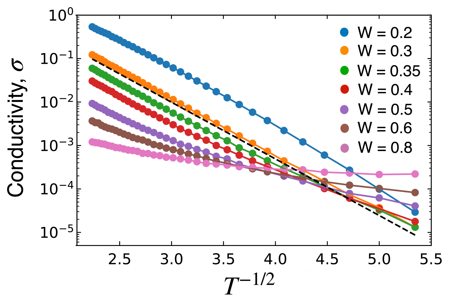
Figure 1: Mott-$1/2$ Law. Numerically computed conductivity $\sigma$ plotted against $T^{-1/2}$ for various disorder strengths $W$ with the energy gap $\Delta=0.3$ (all parameters described later in the text). We observe that the behavior approaches $\ln\sigma\sim-T^{-1/2}$ in the high-temperature limit and agrees with Mott’s theory (straight dashed line) for the widest range of temperatures at $W=0.35$. The numerically computed conductivity deviates from Mott’s relation in the large $W$ limit as the VRH argument is invalidated since too many levels get occupied. Detailed computational discussions on the lattice model will be given in later sections.

In this paper, we present a simple quantum model consisting of an infinite tight-binding chain and on-site disorder potential to model VRH. We apply an electric field to this chain and compute the nonequilibrium Green’s functions in the steady-state limit to study different spectral properties of the disordered system under bias. Since we consider a nonequilibrium steady-state, we introduce dissipators via an infinite fermionic reservoir coupled to each site to drain the energy injected by the electric field. We investigate the signatures of localization by studying the spectral function of a disordered lattice. By increasing the electric field, we demonstrate the localization-delocalization crossover. We also compare our lattice results with those of the coherent potential approximation (CPA) [42, 43, 44] where we calculate the effect of disorder through an effective medium and incorporate it self-consistently into the lattice quantities.

The rest of the paper is organized as follows. In section II, we describe our quantum mechanical model and discuss our calculation methods of Green’s functions and transport properties. In section III, we present our results. For reliable comparison, we briefly discuss the non-disordered lattice case in section III.1. In section III.3 we discuss the disordered lattice case in equilibrium and out of equilibrium. Finally in section IV we discuss our results and conclusions.

II Methods: Disordered Chain under DC bias

We aim to study the electron transport in the bulk limit. As shown in Fig. 2(a), the system is an insulator with dispersion relation $\epsilon_{p}=p^{2}/2m+\Delta$, with the insulating gap $\Delta$ removed from the Fermi energy (set to zero) in equilibrium. To implement the nonequilibrium system with an electric field $E$, one may consider a junction geometry as depicted in Fig. 2(b). However, this junction model leads to finite-size effects that are undesirable for bulk properties. With the number of sites $N$, and the lattice constant $a$ (set to the unit length throughout this work), the bias $V=NEa$ eventually grows to the condition that the source and drain bands do not overlap, especially for a long-chain limit.

For this reason, we construct the nonequilibrium lattice in the bulk limit so that the lattice is translationally invariant in the clean limit. As pictured schematically in Fig. 2(c), we start with an infinite one-dimensional tight-binding chain with a uniform electric field throughout the whole chain. We also introduce fermion reservoir chains that couple to each site of the main chain as shown. The role of the fermion reservoir is to drain the excess energy driven by the electric field and to establish a nonequilibrium steady-state [45]. The Hamiltonian reads as

$$\mathcal{H}= -t\sum_{l=-\infty}^{\infty}(d_{l}^{\dagger}d_{l+1}+d_{l+1}^{\dagger}d_{l})+\sum_{l}\epsilon_{l}d_{l}^{\dagger}d_{l}$$ (4)

$$+\sum_{l\alpha}(\epsilon_{\alpha}-lE)c_{l\alpha}^{\dagger}c_{{l\alpha}}-\frac{g}{\sqrt{L}}\sum_{l\alpha}(c_{l\alpha}^{\dagger}d_{l}+h.c.).$$

Each site of the main chain has the electron creation (annihilation) operator $d^{\dagger}_{l}$ $(d_{l})$ mixing with the reservoir operators $c^{\dagger}_{l\alpha}$ ($c_{l\alpha}$) with the continuum index $\alpha$. $t$ is the tight-binding parameter and $\epsilon_{l}$ the site energy of the main chain. We set $t=1$ as the unit of energy. With the electric field $E$, the site energy at site $l$ is

$$\epsilon_{l}=2t+\Delta+V_{l}-lE.$$ (5)

The Anderson disorder in the active region of the main chain is set by $V_{l}$ with

$$V_{l}=\left\{\begin{array}[]{ll}\mbox{random in }[-W,W]&\mbox{for }-N/2\leq l\leq N/2\\ 0&\mbox{otherwise}\end{array}\right..$$ (6)

In this work, we choose $N=501$, which is large enough to study bulk properties and is computationally feasible to perform finite lattice calculations. The electric field is probed from the lowest value of $E=10^{-4}$ up to $E=0.1$ which typically corresponds to the range of $[10,10^{4}]\text{ kV/cm}$ which includes the typical experimentally relevant range.

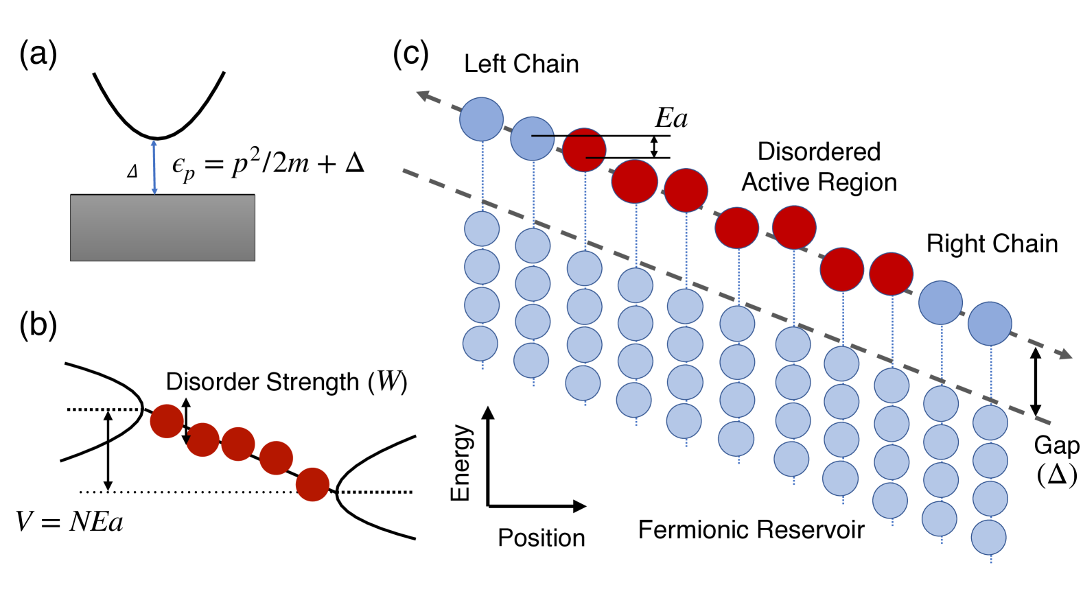
Figure 2: (a) One-dimensional band separated by the gap $\Delta$ from the Fermi level in equilibrium. (b) Disordered chain in junction geometry. While commonly considered, this setup suffers spurious scattering from the band misfit at any electric field as we approach the bulk limit $N\to\infty$ with the chain length $N$. (c) Infinite-chain setup with an electric field. Each site and its reservoir is subject to the electrostatic potential throughout the chain. The central region (red) is disorder-active with the random potential shift in the range $(-W,W)$.

The density of states for the reservoir chain, $L^{-1}\sum_{\alpha}\delta(\omega-\epsilon_{l\alpha})$ with the normalization $L$ for the length of the reservoir chain, is considered structureless and of infinite bandwidth. The electrons on the main chain hybridize with the reservoirs with the hybridization $\Gamma(\omega)=\pi g^{2}L^{-1}\sum_{\alpha}\delta(\omega-\epsilon_{l\alpha})\equiv\Gamma$. The parameter $\Gamma$ accounts for the level broadening and the dissipation rate. The reservoirs are in thermal equilibrium at the bath temperature $T$, with the distribution at site $l$ given by the Fermi-Dirac function $f_{0}(\omega-lE)=[1+e^{(\omega-lE)/T}]^{-1}$ displaced by the electric potential. By using the Keldysh Green’s function method, the effect of the reservoirs can be exactly incorporated as discussed below [46].

II.1 Finite Lattice Calculation

We numerically compute the full retarded Green’s function of the system which is written in an ($N\times N$) matrix form [46] as

$$[\mathcal{G}^{R}(\omega)^{-1}]_{ij} = (\omega-\epsilon_{i}+i\Gamma)\delta_{ij}+t\delta_{|i-j|=1}$$

$$-t^{2}F^{R}_{-}(\omega-NE/2)\delta_{i=j=-N/2}$$

$$-t^{2}F^{R}_{+}(\omega+NE/2)\delta_{i=j=N/2}$$

where the reservoir self-energy is denoted as $-i\Gamma$. The last two terms $t^{2}F^{R}_{-}$, $t^{2}F^{R}_{+}$ are the self-energies of the semi-infinite leads attached respectively to the LHS and RHS of the active sites region (Fig. 2). $F^{R}_{\pm}$ is the retarded local Green’s function at the end site of the left/right semi-infinite chain. These Green’s function of the semi-infinite leads can be computed recursively [46] as

$$F^{R}_{\pm}(\omega)^{-1}=\omega+i\Gamma-(2t+\Delta)-t^{2}F^{R}_{\pm}(\omega\pm E)$$ (8)

The full Green’s function in Eq. (II.1) is computed numerically by inverting the matrix on the RHS with random diagonal terms. We similarly compute the lesser Green’s function numerically as

$$\mathcal{G}^{<}_{ij}(\omega)=\sum_{k=1}^{N}\mathcal{G}^{R}_{ik}(\omega)\Sigma^{<}_{k}(\omega)[\mathcal{G}^{R}_{jk}(\omega)]^{*}$$ (9)

where the lesser self-energy at site $k$ is given as $\Sigma^{<}_{k}(\omega)=2i\Gamma f_{0}(\omega+kE)+t^{2}\delta_{k,-N/2}F^{<}_{-}(\omega-NE/2)+t^{2}\delta_{k,N/2}F^{<}_{+}(\omega+NE/2)$ with $f_{0}(\omega)=[1+e^{\omega/T}]^{-1}$ is the Fermi-Dirac distribution. The lesser Green’s function of the left/right semi-infinite lead is computed recursively over 5000 iterations similar to $F^{R}_{\pm}$ as

$$F^{<}_{\pm}(\omega)=|F^{R}_{\pm}(\omega)|^{2}[2i\Gamma f_{0}(\omega)+t^{2}F^{<}_{\pm}(\omega\pm E)]$$ (10)

In the disordered finite-lattice case ($W\neq 0$), we compute the Green’s functions for $N=501$ active sites. This is then repeated and averaged over 4000 disorder configurations for physical quantities. In the absence of disorder ($W=0$), the Green’s functions satisfy the relation [46]

$${\cal G}^{R,<}_{i,j}(\omega)={\cal G}^{R,<}_{i+k,j+k}(\omega-kE),$$ (11)

and the observable quantities are site-independent. With disorder, the configuration average restores this symmetry away from the edges of the disorder-active region.

II.2 Coherent Potential Approximation (CPA)

To interpret the finite-lattice calculations, we complement them with a simplified result from the coherent potential approximation (CPA). This method has been widely used to study disordered systems, and similar to dynamical mean field theory (DMFT) [47, 48, 49], it uses a local effective medium approximation. Here the inhomogeneous spatial correlations induced by the random disordered potentials are replaced by a local effective medium potential, described as the CPA self-energy, $\Sigma_{CPA}$. This CPA self-energy is determined self-consistently by embedding an impurity in the effective potential and by computing the average disordered Green’s function for multiple impurity configurations and mapping on the effective medium Green’s function. The CPA self-consistent method is summarized as

1. We start with an initial guess for the CPA self-energy as $\Sigma_{\text{CPA}}(\omega)$ often chosen as $\Sigma_{\text{CPA}}(\omega)=0$, we compute the Green’s function of the semi-infinite leads recursively [46] with an electric field $E$. The retarded Green’s function is defined as follows.

   $$[F^{R}_{\pm}(\omega)]^{-1} = \omega+i\Gamma-2t-\Delta$$

   $$-\Sigma^{R}_{\text{CPA}}(\omega)-t^{2}F^{R}_{\pm}(\omega\pm E)$$

   and the lesser Green’s function is defined as

   $$F^{<}_{\pm}(\omega) = |F^{R}_{\pm}(\omega)|^{2}[2i\Gamma f_{0}(\omega)$$

   $$+\Sigma^{<}_{\text{CPA}}(\omega)+t^{2}F^{<}_{\pm}(\omega\pm E)].$$

   We define the total lead-Green’s function as : $F^{R,<}(\omega)=F^{R,<}_{+}(\omega+E)+F^{R,<}_{-}(\omega-E)$ which represents the self energy of the effective medium.

2. We compute the retarded Green’s function excluding the disorder

   $$\mathcal{G}_{0}^{R}(\omega)=[\omega+i\Gamma-2t-\Delta-t^{2}F^{R}(\omega)]^{-1}$$ (14)

   similarly, the lesser Green’s function is calculated as:

   $$\mathcal{G}_{0}^{<}(\omega)=|\mathcal{G}_{0}^{R}(\omega)|^{2}[2i\Gamma f_{0}(\omega)+t^{2}F^{<}(\omega)]$$ (15)

3. We compute the disorder averaged retarded Green’s functions :

   $$G^{R}_{\text{loc}}(\omega)=\langle[{\cal G}^{R}_{0}(\omega)^{-1}-V]^{-1}\rangle_{V}$$ (16)

   and lesser Green’s functions

   $$G^{<}_{\text{loc}}(\omega)=\langle|G^{R}_{\text{loc}}(\omega)|^{2}[2i\Gamma f_{0}(\omega)+t^{2}F^{<}(\omega)]\rangle_{V}$$ (17)

   Disorder averaging in the CPA calculation is defined as $\langle f\rangle_{V}=\int_{-W}^{W}P(V)f(V)dV$ where $P(V)=(2W)^{-1}\Theta(W-|V|)$ is the uniform distribution function of disorder potentials. A detailed discussion of an analytic procedure at zero field is given in Appendix B.

4. We compute the CPA self-energy

   $$\Sigma^{R}_{\text{CPA}}(\omega)=\mathcal{G}^{R}_{0}(\omega)^{-1}-G^{R}_{\text{loc}}(\omega)^{-1}$$ (18)

   $$\Sigma^{<}_{\text{CPA}}(\omega)=\frac{G^{<}_{\text{loc}}(\omega)}{|G^{R}_{\text{loc}}(\omega)|^{2}}-\frac{\mathcal{G}_{0}^{<}(\omega)}{|\mathcal{G}_{0}^{R}(\omega)|^{2}}$$

5. We repeat the above process starting from step 1 until we get a converged solution.

In the next section, we present our results starting with the equilibrium disorder-free case, and we briefly summarize the effect of dissipation $\Gamma$ and temperature $T$. Following that, we present the spectral function of the disordered lattice and compare our results from the lattice calculation and CPA method. In the nonequilibrium case, we discuss the behavior of the Lifshitz tail with the electric field and its effect on localization in the 1D finite lattice by numerically studying the inverse-participation ratio (IPR).

III Results and Discussions

III.1 Disorder-Free Case ($W=0$)

III.1.1 Effect of Damping in Gapped Insulators

We discuss our system in the zero disorder limit and highlight the effect of dissipation $\Gamma$ on the conductivity of the gapped materials. We rigorously compute the effect of damping on the conductivity and the occupation number in the low-temperature limit. An analytic expression for occupation number is computed from the lesser Green’s function as $n_{p}(t)=-iG^{<}_{p}(t,t)$, as detailed in Appendix A. In the limit of $E\rightarrow 0$ the charge excitation per site can be calculated as

$$n_{\rm loc}=\frac{\Gamma}{2\pi}\sqrt{\frac{2m}{\Delta}}$$ (19)

where $m$ is the effective mass of the system and $\Delta$ denotes the gap parameter as mentioned in the previous section. The effective mass $m$ in the continuum model is related to the tight-binding parameter $t$ by $ta^{2}=\hbar^{2}/(2m)$. We can similarly compute the current as

$$J=\int\frac{d\bar{p}}{2\pi}\frac{\bar{p}}{m}n_{\bar{p}}=\frac{\Gamma^{2}E}{16\pi m}\frac{\sqrt{2m\Delta}}{\Delta^{3}}$$

which gives us the DC conductivity as

$$\sigma=\frac{\Gamma^{2}}{16\pi}\frac{\sqrt{2m\Delta}}{m\Delta^{3}}$$ (20)

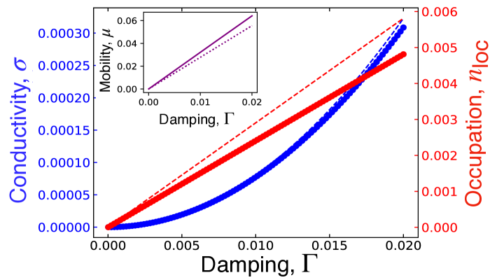
Figure 6: Damping ($\Gamma$) Dependence in low temperature limit ($t=1$, $T=0.01$, $\Delta=0.3$) at zero electric field. The occupation varies linearly with $\Gamma$ (Red curve) and conductivity varies as $\Gamma^{2}$ (blue curve). The theoretical results plotted as the dashed lines seem to follow a similar trend. The inset plot shows Mobility ($\mu=\sigma/n_{\rm loc}$) varying linearly with $\Gamma$ (in purple).

Fig. 6 (in Appendix A) shows the variation of the occupation number and conductivity with damping $\Gamma$ and presents a comparison between our numerical calculation and the analytic derivation. We calculate the mobility ($\mu=\sigma/n_{\rm loc}$) and observe that it increases linearly with the damping $\Gamma$. This is in contrast with the low-field Drude limit result, $\sigma\propto\tau\propto 1/\Gamma$ which was shown in [45] for half-filling. In our model, however, the main chain is kept above the Fermi level by $\Delta$ and scarcely occupied. The lattice is occupied only for a fraction of time proportional to $\Gamma/\Delta$ as shown in Eq. (19), and the time of acceleration due to the electric field is also during the time of occupation, leading to the drift velocity $\propto E\Gamma$. Hence, the conductivity increases as $\Gamma^{2}$ in the absence of disorder.

III.1.2 Equilibrium Case: High-temperature limit

We next study the temperature dependence of transport quantities like the occupation number $n_{\rm loc}$ and the conductivity $\sigma$. The occupation number in the equilibrium limit is obtained from the retarded Green’s function. The occupation number at the wave number $k$ in equilibrium is given as

$$n(k,\omega)=2i\Gamma f_{0}(\omega)|\mathcal{G}^{R}_{k}(\omega)|^{2}$$ (21)

which is integrated over all $\omega$ and $k$ values to obtain the complete expression for occupation as

$$n(T)\approx\sqrt{2mT}e^{-\Delta/T}.$$ (22)

It is also verified numerically in the high-temperature limit, that the occupation of the main chain is independent of the dissipation. Electrons are thermally excited to high enough energies to cross the gap and hence the occupation increases.

In equilibrium, the conductivity has an activation-like behavior (Arrhenius behavior [50]). The conductivity has the empirical form

$$\sigma(\Gamma,T)=\sigma_{0}(\Gamma)e^{-\Delta/T}$$ (23)

The pre-factor depends on $\Gamma$ as $\sigma_{0}\sim\Gamma^{-1}$ which recovers the Drude behavior of conductivity in the high-temperature limit. Thermal excitation is the main source of scattering, and hence only higher energy electrons contribute to the scattering process. As the temperature is lowered, the conductivity deviates from the typical activation behavior since there is lower thermal excitation and electrons do not have enough energy to occupy the band. Hence the few energetic electrons are more likely to be scattered into the reservoir and our behavior coincides with Eq. (20).

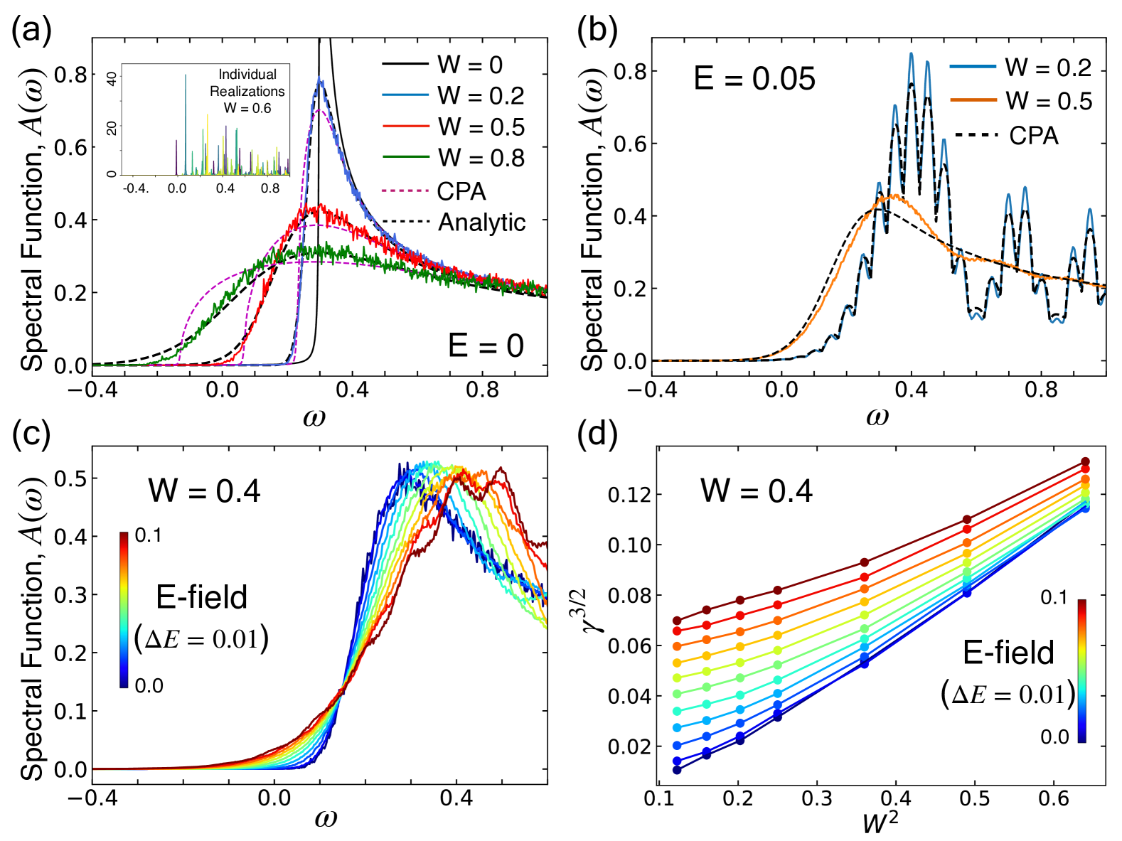
Figure 3: (a) Disorder-averaged spectral function for different values of the disorder $W$ at zero electric field $E=0$ with gap $\Delta=0.3$, $\Gamma=0.0005$ and $T=0.01$ . Pink dashed lines correspond to the spectral function obtained from the CPA calculation which shows a fair match with the lattice calculation but shows no exponential Lifshitz tails. Individual disorder configurations are plotted for $W=0.6$ in the inset which shows distinct localized states. The black solid line is the $1-d$ tight-binding density of states inside the band. (b) Disordered average spectral function at $E=0.05$ for weak ($W=0.2$) and strong ($W=0.6$) disorder. Under the electric field, the system develops slow oscillations which is a modified Airy function, and the fast oscillations are the Wannier Stark peaks occurring at the frequency spacing of $\Delta\omega=E$. At strong disorder, there are no such peaks, indicating that the electric field is not strong enough to break localization. (c) Progression of the Lifshitz tail with electric field at disorder $W=0.4$ for varying electric fields. Starting from the dark-blue curve at zero electric field to the red curve at electric field $E=0.1$ with the spacing $\Delta E=0.01$, the electric field smears the band edge which superposes onto the smearing due to disorder. (d) The decay width of the Lifshitz tail $\gamma$ as a function of $W^{2}$.

III.2 Mott’s $1/2$-Law at Zero E-field

We discuss the linear transport at very low bias (numerically electric field is kept at $E=5\times 10^{-5}$), and verify Mott’s law as previously shown in Fig. 1. In our lattice calculation, we calculate the local current ($J$) at each site [46] using the lesser Green’s function computed from Eq. (9)

$$J_{l}=-t\int[\mathcal{G}^{<}_{l,l+1}(\omega)-\mathcal{G}^{<}_{l+1,l}(\omega)]\frac{d\omega}{2\pi}$$ (24)

The conductivity is computed as $\sigma=J_{l}/E$, which is averaged over many disorder configurations and also over multiple sites to obtain an averaged local conductivity of the lattice. In the absence of disorder, $J_{l}$ is identical on all sites. Fig. 1 demonstrates that $\log(\sigma)$ decreases with $T^{-1/2}$, consistent with the variable range hopping behavior ($\log(\sigma)\propto-T^{-1/2}$ shown as the dashed line for comparison). This provides an important benchmark where Mott’s behavior emerges from a purely quantum mechanical calculation of the Green’s function theory without any reference to Mott’s statistical argument. In the low-temperature limit, the behavior deviates significantly because of the hybridization $\Gamma$ with the fermionic bath.

The Mott behavior as seen in Fig. 1 also varies with the disorder strength as it is observed that the plot deviates from Mott’s scaling (dashed line) both in the high- and the low-disorder limit. At $W\sim\Delta$, $\log(\sigma)$ has the most linear behavior with respect to $T^{-1/2}$. At low disorder strength, the conductivity has slight downward concavity which highlights that conductivity assumes the Arrhenius behavior ($1/T$-dependence). However, at higher disorder strength the conductivity becomes independent of temperature as the levels fall deep in the Fermi sea and localization is too strong for the electrons to hop around. This allows us to identify the VRH regime in our model which typically corresponds to $W\sim\Delta$ in our quantum mechanical calculation of the finite lattice model with disorder. In this limit, the localized levels appear close to the Fermi level which may allow electrons to hop into the unoccupied band. The range of the VRH regime will be further discussed in the following sections.

III.3 Disordered Lattice under E-field

The highlight of this study is the discussion of localization in a disordered tight-binding chain and the effect of an electric field on Anderson localization. It is known that in a 1D system, any amount of disorder can lead the system into localization [5, 21]. The averaged disordered spectral function is computed from the diagonal elements of the imaginary part of Eq. (II.1) and plotted in Fig.3. Averaging over multiple disorder configurations, the spectral function becomes smooth and the band edge shifts. We observe not only the broadening of the band with increasing disorder but also the exponential Lifshitz tail appearing along the edge of the band. Our numerically computed spectral function is an accurate match for the analytic expression of the spectral function [depicted as the black curves in Fig. 3(a) reported in previous studies [24]. The inset shows individual disorder realizations for some disorder strength which shows localized levels marked by $\delta$-function-like spikes in the DOS.

We compare our finite-lattice calculations with the CPA calculation (shown in pink dashed lines) at zero field in Fig. 3(a). The disorder-averaged spectral function shows remarkable similarity to the CPA calculation. This is an important benchmark for both the finite lattice and the CPA calculations as we can highlight some key aspects of both approaches. CPA being a single-site approximation replaces the inhomogeneity of a disordered lattice with an averaged coherent potential. Hence, it does not show any Anderson localization but highlights the broadening of the band as a result of the scattering of the complex potential. In contrast to the CPA-averaged spectral function, the finite lattice spectral function forms a Lifshitz tail rather than a sharp band edge. With its inability to account for the Anderson localization, the CPA method shows no such exponential tail. In the high-field limit, however, the non-local effects of the disorder become disentangled, the CPA becomes more reliable, and its agreement with the finite-lattice calculations is excellent as shown in Fig. 3(b).

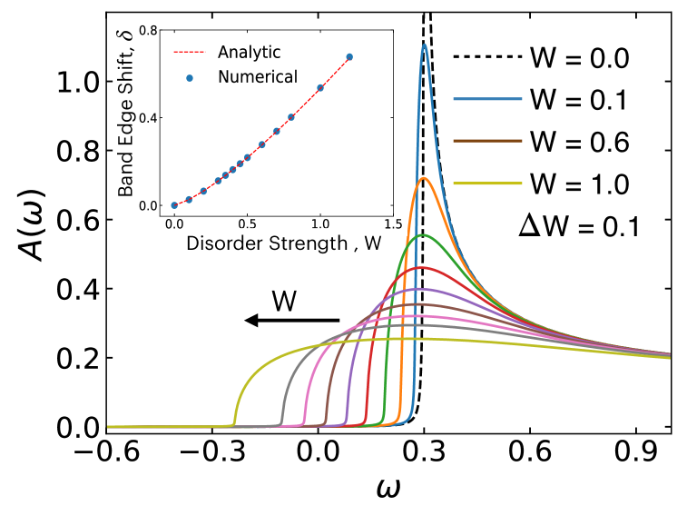
Figure 4: CPA spectral function at $\Gamma=0$ and $E=0$ with varying disorder strengths. In the inset, the band edge shift is compared between the finite-lattice calculation and the analytical CPA results.

In Fig. 3(b-d), we show the effect of the electric field on the spectral properties of the disordered chain. Applying the electric field to the disordered chain results in the spectral function developing oscillations which indicate the tendency for the system to get delocalized. At a very strong electric field and low disorder strength, Anderson localization crosses over to weak localization which is depicted as Wannier Stark peaks in Fig. 3(b) occurring with the frequency interval of $\Delta\omega=E$. This is in agreement with some of the earlier works [10] which have mentioned that the electric field delocalizes the system.

Fig. 3(b) shows two oscillation periods in the spectra. The slow oscillation represents the Airy function envelope as can be seen in a continuum model. The Airy function envelope decays near the band edge as the electronic wave functions smear into the energetically forbidden zone. This spectral behavior, coincidentally, is of similar mathematical form to the exponential decay of Lifshitz tail due to the disordered potential [22, 23]. Applying the electric field further extends the Lifshitz tails into the gap as seen from Fig. 3(c). Combining the two limits of $(W>0,E=0)$ and $(W=0,E>0)$, we propose an empirical expression for this exponential Lifshtiz tail for non-zero disorder and electric field as

$$A(\omega)\sim\exp\left[-\left|\frac{\omega-\Delta+\delta}{\gamma}\right|^{3/2}\right]$$ (25)

below the band edge, where $\gamma$ is the decay width and $\delta$ represents the band edge shift. We discuss the behavior of both of these variables for varying disorder strengths and highlight the key underlying physics.

From the earlier analytic studies of Lifshtiz tails [22, 23], the decay of the Lifshitz tail $\gamma$ scales with respect to the $W$ as $\gamma^{3/2}\propto W^{2}$ at $E=0$ (blue-black) as shown in Fig. 3(d). At higher electric fields, $\gamma$ tends to deviate from this scaling behavior. At zero disorder and at a finite field, the spectral tail is given in terms of the Airy function solution, $\gamma\propto E^{2/3}$ [51]. Therefore, the tail length $\gamma$ is proposed to the form

$$\gamma=\max\left[\left(\frac{3W^{2}}{16\sqrt{t}}\right)^{2/3},\left(\frac{3eEa\sqrt{t}}{4}\right)^{2/3}\right].$$ (26)

The extension of the Lifshtiz tail implies that randomly occurring localized levels would penetrate into the Fermi sea facilitating electron excitations into the main chain and would affect the transport properties of the disordered systems.

The bandshift $\delta$ is important to understand the criterion for the VRH regime, and it is well captured by the CPA method. This is depicted in Fig. 4 where the band edge shifts to lower energy with increasing disorder strength. We analytically derive the band edge shift at zero field using the local averaged Green’s function, $G^{R}_{\rm loc}(\omega)$ in Eq. (16) as a function of the disorder strength, which is shown in the Appendix B. In Fig. 4 we show the band edge crosses the Fermi level at disorder $W\approx 2\Delta=0.6$, where this system typically develops metallic characteristics. In the finite-lattice calculations, the crossing happens at a slightly lower value $W^{*}\sim 0.5$ due to the Lifshitz tail crossing over the Fermi level. This discrepancy for the threshold disorder becomes more important in transport behavior.

One of the major questions that we address in this work is the effect of an electric field on Anderson localization. To this end, we compute the inverse participation ratio (IPR) [52] which is typically defined as the fourth power of a normalized eigenfunction $\phi_{i}$ summed over all spatial indices $i$ as

$$\text{IPR}=\sum_{i}^{N}|\phi_{i}|^{4}$$

for a system of size $N$. This method gives us insights into spatial localization or distribution of wavefunctions in a lattice. The IPR for an extended state in 1D typically is $\sim 1/N$ and it increases as the localization increases. In an open system, we define the IPR through the Green’s function as

$$\text{IPR}=\frac{\sum_{x=1}^{M}|\mathcal{G}^{R}(x,\omega=-xE)|^{4}}{(\sum_{x=1}^{M}|\mathcal{G}^{R}(x,\omega=-xE)|^{2})^{2}}$$ (27)

where $\mathcal{G}^{R}(x,\omega)$ is the local retarded Green’s function at position $x$ as computed in the Eq. (II.1). The denominator provides the normalization and makes the IPR dimensionless. The IPR values are computed at the local Fermi level which provides the main contribution to the transport.

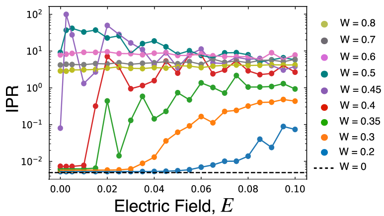
Figure 5: Inverse-participation-ratio (IPR) plotted against electric field $E$. $\Gamma=0.0005$, $N=501$, $t=1$, $T=0.01$. The dashed line represents the $\text{IPR}\sim 1/N$ at zero disorder. Observe that in the disorder limit $\Delta<W<W^{*}$ the IPR at the Fermi level shows a sharp rise with $W$ as the electric field allows localized levels to penetrate into the Fermi sea. After the sharp rise, the electric field gradually delocalizes the system. At $W>W^{*}$, the IPR is independent of the electric field as localization is far too strong to be affected by the electric field.

Fig. 5 shows the evolution of the IPR as a function of the electric field at different disorder values $W$. It is observed that in the zero disorder limit (shown as a dashed line) we recover the $1/N$ behavior showing that the states are all extended. At low disorder, the IPR increases gradually as the electric field increases. We observe weak localization of electronic levels and the exponential part of the density of states smears into the gap and falls into the Fermi level due to the effect of the electric field. Now, increasing the disorder strength in the range

$$\Delta<W<W^{*},$$ (28)

the gradual rise in IPR becomes a much sharper increase with $W$ as the strongly localized levels are detected at the Fermi level. The upper limit $W^{*}=0.5$ (at $\Delta=0.3$) coincides with the condition that the Lifshitz tail crosses the Fermi energy, as discussed in Fig. 3. The CPA gives a slight overestimation of $W^{*}$ at $W^{*}\approx 2\Delta$. Near $W\approx W^{*}$, the IPR gradually decreases with increasing electric field, which indicates gradual delocalization due to the electric field. This is in agreement with what has been mentioned in earlier works [29] for the case of a discontinuous disorder. In the strong disorder limit, $W>W^{*}$, localization is too strong to be broken by the electric field as observed by the flattening of the IPR with respect to the electric field.

IV Conclusion

In this work, we analyzed the spectral properties of a disordered tight-binding chain under a DC electric field and coupled it to a dissipative bath, where the Fermi level is kept below the band edge. When disorder is present in the system, we observe typical Anderson localization. The spectral behavior of the localized system is characterized by using two different methods, one with an infinite lattice with a finite disorder-active region, and the second approach with the coherent potential approximation.

We first verify Mott’s law of the variable range hopping conductivity in the linear transport regime for our quantum mechanical model. This is one of the key results of this work, as we can obtain Mott’s phenomenological model from quantum mechanical principles without resorting to statistical arguments. The finite-lattice calculation, in the strong electric field regime, successfully captures exponential Lifshitz tails which indicate the presence of localized levels beyond the allowed potential fluctuation bounds. We find that the electric field delocalizes a disordered system and allows for the system to crossover from Anderson localization to the Bloch oscillations.

Appendix A Linear Transport in a Clean Insulator

We present an analytic theory for electron transport in a band separated from the Fermi energy by $\Delta$ with the dispersion relation

$$\epsilon(p)=\Delta+\frac{p^{2}}{2m}.$$ (29)

In the following analytic derivations, we employ the temporal gauge for the electric field by replacing the momentum $p$ by $p+eEt$ $(e=1)$ without the voltage slope in the potential as used in the numerical calculations [53]. With the damping parameter $\Gamma$ provided by the coupling to the particle reservoir, the retarded Green’s function under a uniform DC electric field $E$ is given as

$$G^{R}_{p}(t_{2},t_{1})=-i\theta(t_{2}-t_{1})e^{-\Gamma|t_{2}-t_{1}|}\exp\left[-i\int^{t_{2}}_{t_{1}}\epsilon(p+Es)ds\right].$$ (30)

With the average time $T=(t_{2}+t_{1})/2$ and the relative time $t=t_{2}-t_{1}$, we write

$$G^{R}_{p}(t,T)=-i\theta(t)e^{-\Gamma|t|}\exp\left[-i\int^{T+t/2}_{T-t/2}\epsilon(p+Es)ds\right].$$ (31)

In the steady-state limit, the lesser Green’s function $G^{<}_{p}(t_{2},t_{1})$ can be expressed as

$$G^{<}_{p}(t,T)=\int ds_{1}\int ds_{2}G^{R}_{p}(t_{2},s_{2})\Sigma_{0}^{<}(s_{2}-s_{1})[G^{R}_{p}(t_{1},s_{1})]^{*},$$ (32)

with the dissipative (lesser) self-energy from the bath, $\Sigma_{0}^{<}(s)$ obtained as the Fourier transform of $\Sigma_{0}^{<}(\omega)=2i\Gamma\theta(-\omega)$ at zero temperature, as

$$\Sigma_{0}^{<}(s)=2i\Gamma\int_{-\infty}^{0}e^{-i\omega s+\eta\omega}\frac{d\omega}{2\pi}=-\frac{\Gamma}{\pi(s+i\eta)}.$$ (33)

After a lengthy but straightforward calculation, we get

$$G_{p}^{<}(t) = -\frac{\Gamma}{\pi}e^{-i\epsilon(p)t-i\frac{E^{2}t^{3}}{24m}}\int_{-\infty}^{0}ds_{1}\int_{-\infty}^{0}ds_{2}\frac{e^{2\Gamma S}}{s+t+i\eta}\times$$ (34)

$$\exp\left[i(t+s)\epsilon(p+ES)+i\frac{E^{2}(s+t)^{3}}{24m}\right].$$

The average time $T$ dependence always appears in the combination of $p+ET$, which is the manifestation of the gauge-invariance, and we replace $p+ET$ by the gauge-covariant momentum $p$ and the above steady-state expression results. Here, $S=(s_{2}+s_{1})/2$ is the average time and $s=s_{2}-s_{1}$ is the relative time. For the occupation number of the band at the electric field $E$, we have $n_{p}=-iG^{<}_{p}(t=0)$ and

$$n_{p}(E) = \frac{i\Gamma}{\pi}\int_{-\infty}^{\infty}ds\int_{-\infty}^{-|s|/2}dS\frac{e^{2\Gamma S}}{s+i\eta}\times$$ (35)

$$\times \exp\left[is\epsilon(p+ES)+\frac{iE^{2}s^{3}}{24m}\right].$$

In the zero field limit, the total population in the band becomes

$$n_{0}=\int_{-\infty}^{\infty}n_{p}\frac{dp}{2\pi}=\frac{i}{4\pi^{2}}\int dp\int_{-\infty}^{\infty}ds\frac{e^{-\Gamma|s|+i\epsilon(p)s}}{s+i\eta},$$ (36)

which after some contour integrals becomes

$$n_{0}=\frac{1}{2\pi^{2}}\int_{-\infty}^{\infty}dp\tan^{-1}\left(\frac{\Gamma}{\epsilon(p)}\right)\approx\frac{\Gamma}{2\pi}\sqrt{\frac{2m}{\Delta}},$$ (37)

in the small $\Gamma$ limit, Eq. (19).

For the current at a finite electric field, we compute the current similarly. The total momentum from the band becomes

$$\int pn_{p}\frac{dp}{2\pi} = \frac{i\Gamma}{\pi}\int\frac{dp}{2\pi}p\int_{-\infty}^{\infty}ds\int_{-\infty}^{-|s|/2}dS\frac{e^{2\Gamma S}}{s+i\eta}\times$$ (38)

$$\times \exp\left[is\epsilon(p+ES)+\frac{iE^{2}s^{3}}{24m}\right],$$

which becomes in the leading order of $E$ with the change of variable $p+ES\to p$. After performing an integral over $S$, the leading order of $E$ to the current becomes

$$\frac{iE}{8\pi^{2}\Gamma}\int dp\int_{-\infty}^{\infty}ds\frac{1+\Gamma|s|}{s+i\eta}e^{-\Gamma|s|+i\epsilon(p)s}$$ (39)

$$= \frac{E}{4\pi^{2}\Gamma}\int dp\left[\tan^{-1}\frac{\Gamma}{\epsilon(p)}-\frac{\Gamma\epsilon(p)}{\Gamma^{2}+\epsilon(p)^{2}}\right].$$

Taking the leading order contribution in $\Gamma$, we have the linear electric current

$$J=\int\frac{p}{m}n_{p}\frac{dp}{2\pi}\approx\frac{\Gamma^{2}E}{6\pi^{2}m}\int\frac{dp}{\epsilon(p)^{3}}=\frac{\Gamma^{2}E}{8\pi\sqrt{2m\Delta^{5}}},$$ (40)

and the DC conductivity $\sigma=J/E$ as in Eq. (20)

$$\sigma=\frac{\Gamma^{2}}{8\pi\sqrt{2m\Delta^{5}}}.$$ (41)

We obtain the mobility $\mu=\sigma/n$ as

$$\mu=\frac{\Gamma}{8m\Delta^{2}}.$$ (42)

Interpreting this result in terms of the Drude theory $\mu=\tau/m$ with the scattering time $\tau$, we arrive at a surprising result $\tau=\Gamma/(8\Delta^{2})$ in which the scattering time is proportional to the scattering rate. This is due to the fact that the band is only occasionally occupied with the probability proportional to $(\Gamma/\Delta)^{2}$ through hybridizing with the particle reservoir and that the electrons accelerate from rest when they re-enter the band from the baths. Therefore the mobility is proportional to $(\Gamma/\Delta)^{2}\cdot\Gamma^{-1}$, being consistent with the Drude interpretation.

Appendix B Band Shift in the Coherent Potential Approximation (CPA) at Zero Field

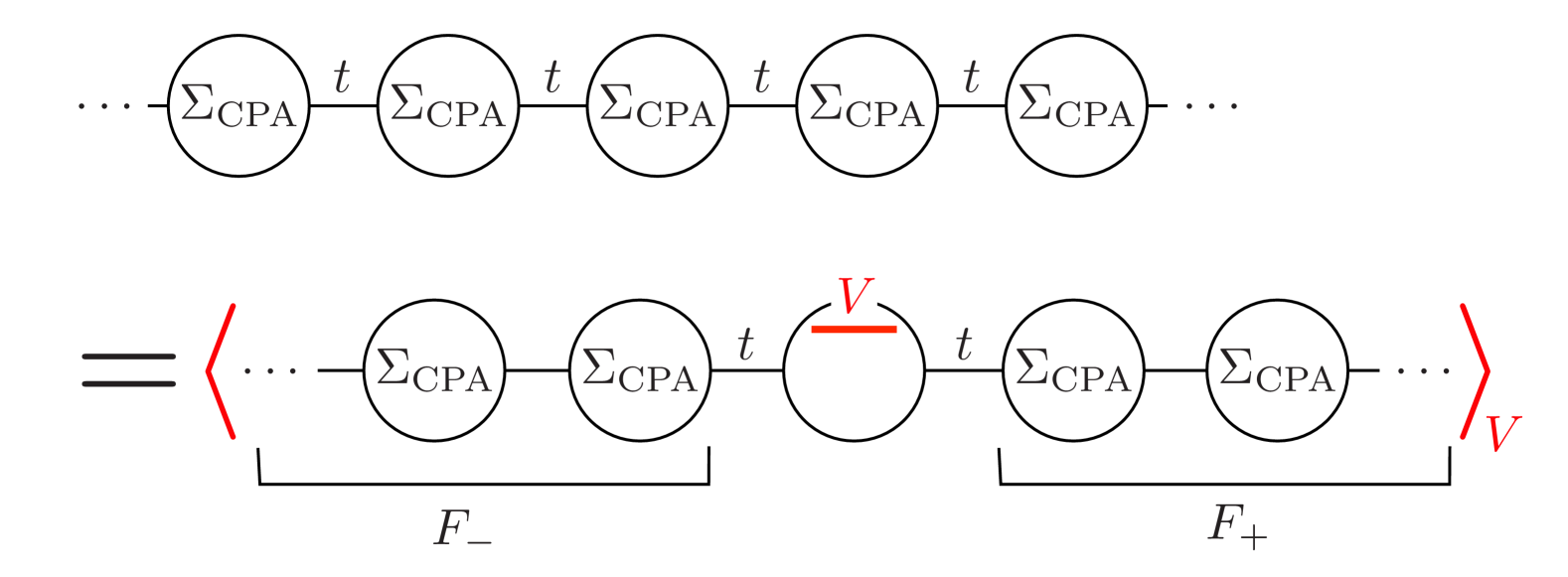
Figure 7: Schematic CPA self-consistent condition. The translationally invariant lattice with the self-energy $\Sigma_{\rm CPA}$ is equivalent to the impurity-level averaging over $V$ (denoted as red) on a chosen site with remaining sites with the embedded self-energy $\Sigma_{\rm CPA}$.

In the CPA, the effect of the disorder is represented by a self-energy $\Sigma_{\rm CPA}(\omega)$ that encodes the level shift and the dephasing from the scattering, as schematically shown in FIG. 7. We consider the level-disorder where the local orbital energy is randomly shifted by $V\in[-W,W]$ set by the disorder strength $W$. The local retarded Green’s function (first line in FIG. 7) in a one-dimensional chain is

$$G^{R}_{\rm loc}(\omega)=\int\frac{dk}{2\pi}\frac{1}{\omega-\epsilon_{k}-\Sigma_{\rm CPA}(\omega)},$$ (43)

with the tight-binding dispersion relation $\epsilon_{k}=-2t\cos k$. Here, we set the damping $\Gamma\to 0$ for convenience. The second line in FIG. 7 represents the disorder averaged local Green’s function. The disorder-specific Green’s function has the leads of semi-infinite chains with the same self-energy $\Sigma_{\rm CPA}$ and the disorder shift $V$, as

$$G^{R}_{V}(\omega)=\frac{1}{\omega-V-2t^{2}F^{R}(\omega)},$$ (44)

where $F^{R}(\omega)$ is the Green’s function at the edge site that connects to the central site for each semi-infinite chain. The factor 2 is due to the sum of the left- and right-chains, $F_{-}$ and $F_{+}$, respectively. At zero bias, $F_{+}=F_{-}\equiv F$. The $F$-Green’s functions in one-dimension can be obtained recursively [46] as

$$F^{R}_{\pm}(\omega)=[\omega+i\eta-\Sigma_{\rm CPA}(\omega)-t^{2}F^{R}_{\pm}(\omega)]^{-1}.$$ (45)

The CPA is to equate both sides after the local averaging over the disorder $V$ is performed locally,

$$G^{R}_{\rm loc}(\omega)=\langle G^{R}_{V}(\omega)\rangle_{V}=\int^{W}_{-W}\frac{dV}{2W}G^{R}_{V}(\omega).$$ (46)

The CPA problem, Eqs. (43-46), can be solved exactly at zero bias. The $V$-integral can be performed exactly as

$$G^{R}_{\rm loc}(\omega)=\frac{1}{2W}\log\left|\frac{\omega+W-2t^{2}F(\omega)}{\omega-W-2t^{2}F(\omega)}\right|.$$ (47)

Eq. (43) can be rewritten in the 1-$d$ chain as

$$G^{R}_{\rm loc}(\omega)=\frac{1}{\omega-\Sigma_{\rm CPA}(\omega)-2t^{2}F(\omega)}.$$ (48)

From Eq. (45), we may eliminate $\Sigma_{\rm CPA}$ and have the self-consistent relation $f(F)=0$ with

$$f(F)=\frac{1}{-t^{2}F+F^{-1}}-\frac{1}{2W}\log\left|\frac{\omega+W-2t^{2}F}{\omega-W-2t^{2}F}\right|.$$ (49)

By finding the root of the equation $f(F)=0$ per given set $(\omega+i\eta,W)$ we can solve the problem. To evaluate the band edge shift, we note that the spectral weight of the retarded Green’s function goes to zero outside the band, i.e. any real root $F$ does not exist. Therefore, at the band edge we require simultaneously $f(F)=0$ and $f^{\prime}(F)=0$, which sets a condition for a critical value $\omega=\omega_{c}$ at a given $W$. By combining the conditions, we obtain

$$\omega_{c}-2t^{2}F_{c} = g(W,F_{c})$$ (50)

$$\frac{F_{c}}{1-t^{2}F_{c}^{2}} = -\frac{1}{2W}\log\left|\frac{g(W,F_{c})+W}{g(W,F_{c})-W}\right|$$ (51)

with $g(W,F_{c})=[W^{2}+2t^{2}(1-t^{2}F_{c}^{2})^{2}/(1+t^{2}F_{c}^{2})]^{1/2}$ and $F_{c}=F(\omega_{c})$. In the $W\to 0$ limit, $\omega_{c}=-2t$ becomes the lower band edge and the solution is $tF_{c}=-1$. Therefore, for a given $W$, we solve for $F_{c}$ from Eq. (51) in the neighborhood of $tF_{c}=-1$ and obtain $\omega_{c}$ from Eq. (50) for the bande dge shift $\delta$. This analytic solution agrees with the numerical CPA solution very well as shown in FIG. 4.

References

- Anderson [1958] P. W. Anderson, Phys. Rev. 109, 1492 (1958).
- Lee and Ramakrishnan [1985] P. A. Lee and T. V. Ramakrishnan, Rev. Mod. Phys. 57, 287 (1985).
- Mott [1967] N. Mott, Advances in Physics 16, 49 (1967).
- Mott [1968a] N. F. Mott, The Phil. Mag. 17, 1259 (1968a).
- Thouless [1974] D. Thouless, Physics Reports 13, 93 (1974).
- Kramer and MacKinnon [1993] B. Kramer and A. MacKinnon, Rep. Prog. Phys. 56, 1469 (1993).
- Anderson [2010] P. Anderson, 50 Years of Anderson Localization, Published by World Scientific Publishing Co. Pte. Ltd (2010).
- Cutler and Mott [1969] M. Cutler and N. F. Mott, Phys. Rev. 181, 1336 (1969).
- Sheng [1990] P. Sheng, Scattering and localization of classical waves in random media, Vol. 8 (World Scientific, 1990).
- Kirkpatrick [1985] T. R. Kirkpatrick, Phys. Rev. B 31, 5746 (1985).
- John [1984] S. John, Phys. Rev. Lett. 53, 2169 (1984).
- Lagendijk et al. [2009] A. Lagendijk, B. v. Tiggelen, and D. S. Wiersma, Physics Today 62, 24 (2009).
- Wiersma et al. [1997] D. S. Wiersma, P. Bartolini, A. Lagendijk, and R. Righini, Nature 390, 671 (1997).
- Schwartz et al. [2007] T. Schwartz, G. Bartal, S. Fishman, and M. Segev, Nature 446, 52 (2007).
- Segev et al. [2013] M. Segev, Y. Silberberg, and D. N. Christodoulides, Nat. Photonics 7, 197 (2013).
- Rothstein [2013] I. Z. Rothstein, Phys. Rev. Lett. 110, 011601 (2013).
- Tian [2019] Z. Tian, ACS Nano 13, 3750 (2019).
- Mafi et al. [2019] A. Mafi, J. Ballato, K. W. Koch, and A. Schülzgen, J Lightwave Technology 37, 5652 (2019).
- Mott et al. [1975] N. F. Mott, M. Pepper, S. Pollitt, R. H. Wallis, and C. J. Adkins, Proc. of the Royal Soc. of London. A. Math. and Phys. Sci. 345, 169 (1975).
- Mott [1971] N. F. Mott, Phil. Mag. 24, 911 (1971).
- Mott and Twose [1961] N. Mott and W. Twose, Advances in Physics 10, 107 (1961).
- Halperin [1965] B. I. Halperin, Phys. Rev. 139, A104 (1965).
- Garcia and Hofmann [2024] E. R. Garcia and J. Hofmann, Phys. Rev. E 109, L032103 (2024).
- Van Mieghem [1992] P. Van Mieghem, Rev. Mod. Phys. 64, 755 (1992).
- Lee et al. [1983] Y. C. Lee, C. S. Chu, and E. Castaño, Phys. Rev. B 27, 6136 (1983).
- Soukoulis et al. [1983] C. M. Soukoulis, J. V. José, E. N. Economou, and P. Sheng, Phys. Rev. Lett. 50, 764 (1983).
- Prigodin [1980] V. Prigodin, Zh. Eksp. Teor. Fiz 79, 2338 (1980).
- Kirkpatrick [1986] T. R. Kirkpatrick, Phys. Rev. B 33, 780 (1986).
- Prigodin and Altshuler [1989] V. N. Prigodin and B. L. Altshuler, Phys. Lett. A 137, 301 (1989).
- Bleibaum et al. [1995] O. Bleibaum, H. Böttger, V. V. Bryksin, and P. Kleinert, Phys. Rev. B 52, 16494 (1995).
- Bleibaum and Belitz [2004] O. Bleibaum and D. Belitz, Phys. Rev. B 69, 075119 (2004).
- Mott [1968b] N. F. Mott, J. Non-Cryst. Solids 1, 1 (1968b).
- Miller and Abrahams [1960] A. Miller and E. Abrahams, Phys. Rev. 120, 745 (1960).
- Shklovskii [2024] B. I. Shklovskii, Low Temp. Phys. 50, 1101 (2024).
- Lee [1984] P. A. Lee, Phys. Rev. Lett. 53, 2042 (1984).
- Shklovskii and Efros [2013] B. I. Shklovskii and A. L. Efros, Electronic properties of doped semiconductors, Vol. 45 (Springer Science & Business Media, 2013).
- Epstein et al. [2001] A. Epstein, W.-P. Lee, and V. Prigodin, Syn. Met. 117, 9 (2001).
- Apsley and Hughes [1974] N. Apsley and H. P. Hughes, Philosophical Magazine 30, 963 (1974).
- Liu et al. [2010] H. Liu, A. Pourret, and P. Guyot-Sionnest, ACS Nano 4, 5211 (2010).
- Paasch et al. [2002] G. Paasch, T. Lindner, and S. Scheinert, Synthetic Metals 132, 97 (2002).
- Evans et al. [2017] H. A. Evans, J. G. Labram, S. R. Smock, G. Wu, M. L. Chabinyc, R. Seshadri, and F. Wudl, Inorg. Chem. 56, 395 (2017).
- Elliott et al. [1974] R. J. Elliott, J. A. Krumhansl, and P. L. Leath, Rev. Mod. Phys. 46, 465 (1974).
- Janiš [2021] V. Janiš, arXiv preprint arXiv:2109.04723 (2021).
- Dohner et al. [2022] E. Dohner, H. Terletska, K.-M. Tam, J. Moreno, and H. F. Fotso, Phys. Rev. B 106, 195156 (2022).
- Han [2013] J. E. Han, Phys. Rev. B 87, 085119 (2013).
- Li et al. [2015] J. Li, C. Aron, G. Kotliar, and J. E. Han, Phys. Rev. Lett. 114, 226403 (2015).
- Aoki et al. [2014] H. Aoki, N. Tsuji, M. Eckstein, M. Kollar, T. Oka, and P. Werner, Rev. Mod. Phys. 86, 779 (2014).
- Georges et al. [1996] A. Georges, G. Kotliar, W. Krauth, and M. J. Rozenberg, Rev. Mod. Phys. 68, 13 (1996).
- Fotso and Freericks [2020] H. F. Fotso and J. K. Freericks, Front. Phys. 8, 10.3389/fphy.2020.00324 (2020).
- Yuen et al. [2009] J. D. Yuen, R. Menon, N. E. Coates, E. B. Namdas, S. Cho, S. T. Hannahs, D. Moses, and A. J. Heeger, Nat. Mat. 8, 572 (2009).
- Schwinger et al. [2001] J. Schwinger, B.-G. Englert, et al., Quantum mechanics: symbolism of atomic measurements, Vol. 1 (Springer, 2001).
- Antipov et al. [2016] A. E. Antipov, Y. Javanmard, P. Ribeiro, and S. Kirchner, Phys. Rev. Lett. 117, 146601 (2016).
- Chen and Han [2024] X. Chen and J. E. Han, Phys. Rev. B 109, 054307 (2024).