Simple and accurate approximations to the Riemann zeta function

Abstract

We develop approximations for the Riemann zeta function that enable high-precision computation within the critical strip and other vertical strips. These approximations combine the main sum of the Riemann-Siegel formula with a simple approximation of the remainder term, which involves only elementary functions and certain precomputed coefficients obtained via Gaussian quadrature. Additionally, we provide approximations for the derivative of the Riemann zeta function and present extensive numerical evidence demonstrating the accuracy of these approximations.

Keywords: Riemann zeta function, Riemann-Siegel formula, Gaussian quadrature, high-precision algorithm 2020 Mathematics Subject Classification : Primary 11M06, Secondary 11Y35

1 Introduction and main results

There exist many methods for computing the Riemann zeta function. One of the simplest is the Euler-Maclaurin summation method [3, 12, 22], which is easy to implement, provides rigorous error bounds, and allows for high-precision computation of $\zeta(s)$. However, a major drawback of this method is that it requires summing of $O(|s|)$ terms, making it impractical for large values of $s$. Another highly efficient algorithm, developed by Borwein [4], also has rigorous error bounds and enables high-precision computation of $\zeta(s)$ when $\textnormal{Im}(s)$ is not large.

For values of $s$ with $\textnormal{Im}(s)$ large, the preferred method is the Riemann-Siegel formula and its various extensions. The original Riemann-Siegel formula [3, 6, 22, 23] was developed for computing $\zeta(s)$ on the critical line $\textnormal{Re}(s)=1/2$. It consists of the main sum of $N_{t}:=\lfloor\sqrt{t/(2\pi)}\rfloor$ terms (here and throughout this paper we denote $s=\sigma+{\textnormal{i}}t$ and assume that $t>0$) and a remainder term, which can be expressed in terms of certain integrals or expanded as asymptotic series. Keeping the first $j$ terms of this asymptotic series results in an error $O(t^{-\frac{1}{4}-\frac{j}{2}})$ (see [6] for rigorous and effective upper bounds for these errors). A lot of work was done on extending and improving the Riemann-Siegel formula. Odlyzko and Schönhage [19] introduced a fast algorithm for evaluating $\zeta(s)$ at multiple points, which is particularly useful for locating the zeros of the Riemann zeta functon on the critical line. Hiary [9] developed an algorithm that reduces the complexity of evaluating $\zeta(1/2+{\textnormal{i}}t)$ at a single point to $O(t^{4/13+o(1)})$, compared to the standard Riemann-Siegel formula’s complexity of $O(t^{1/2})$. A simpler version of Hiary’s algorithm [9] achieves complexity $O(t^{1/3+o(1)})$ with minimal memory requirement. Another algorithm due to Hiary [10] produces Riemann-Siegel-type approximations (requiring $O(t^{1/2+o(1)})$ terms) by starting from the Euler-Maclaurin formula. Smoothed versions of the Riemann-Siegel formula have been derived in [2, 15, 21, 22] and a Riemann-Siegel-type formula for computing $\zeta(s)$ for general values of $s$ (not necessarily on the criticial line) was developed in [5].

In this paper we construct approximations to $\zeta(s)$ that are valid in arbitrary vertical strips, including the critical strip. Our method is conceptually similar to the approach of Galway [7], whose algorithm computes $\zeta(s)$ by numerically evaluating the integrals that appear in the error term of the Riemann-Siegel formula. Galway’s approximations can yield highly accurate results, but their implementation requires careful tuning, as they depend on three parameters $\{z_{1},z_{2},M\}$ that must be appropriately chosen to achieve the best accuracy. In contrast, our approximations depend on a single integer parameter $p$ along with certain precomputed coefficients $\{\omega_{p,j}\}_{0\leq j\leq p}$ and $\{\lambda_{p,j}\}_{1\leq j\leq p}$. Our approximations allow for high-precision computation of $\zeta(s)$ within the critical strip and other vertical strips. High-precision computations of the Riemann zeta function are not just of theoretical interest; they can lead to significant mathematical discoveries. For example, computations of the notrivial zeros of $\zeta(s)$ to high precision was the crucial ingredient in the disproof of Merten’s conjecture [20].

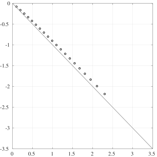
(a)

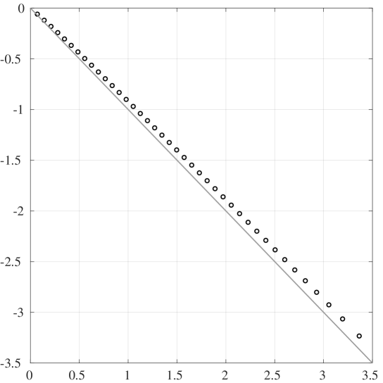
(b)

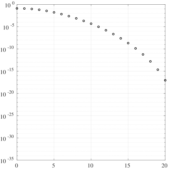
(c)

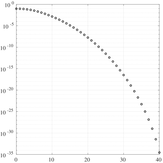
(d)

Figure 1: The numbers $\lambda_{p,j}$ and $|\omega_{p,j}|$ for $p\in\{20,40\}$.

The key components in our approximations for the Riemann zeta function are the $2p+1$ complex numbers $\{\omega_{p,j}\}_{0\leq j\leq p}$ and $\{\lambda_{p,j}\}_{1\leq j\leq p}$. We explain in Section 2 how these numbers are derived. We have precomputed $\omega_{p,j}$ and $\lambda_{p,j}$ to sufficiently high precision for all $1\leq p\leq 30$ and for many values of $p$ in the range $p\leq 150$; the results can be downloaded from the author’s webpage. The values of $\omega_{p,j}$ and $\lambda_{p,j}$ for $p\in\{5,8,10\}$ are listed in Appendices A and B. To illustrate the magnitude and the distribution of these numbers in the complex plane, Figure 1 displays $\lambda_{p,j}$ and $|\omega_{p,j}|$ for $p\in\{20,40\}$. We observe that these numbers are not large in magnitude, that $\lambda_{p,j}$ lie slightly above the ray $\arg(z)=-\pi/4$ and that $|\omega_{p,j}|$ decay rapidly as $j$ increases.

Given the numbers $\{\omega_{p,j}\}_{0\leq j\leq p}$ and $\{\lambda_{p,j}\}_{1\leq j\leq p}$, we define

$${\mathcal{I}}_{M,p}(s):=\omega_{p,0}M^{-z}+\sum\limits_{j=1}^{p}\omega_{p,j}\Big{[}e^{-2\pi M\lambda_{p,j}}\big{(}M+{\textnormal{i}}\lambda_{p,j}\big{)}^{-s}+e^{2\pi M\lambda_{p,j}}\big{(}M-{\textnormal{i}}\lambda_{p,j}\big{)}^{-s}\Big{]},$$ (1)

where $M>0$ and $s\in{\mathbb{C}}$. For a function $f:{\mathbb{C}}\mapsto{\mathbb{C}}$ we denote

$$\bar{f}(s):={\overline{f(\bar{s})}}.$$ (2)

Clearly, if $f$ is an entire function of $s$, then so is $\bar{f}$. For $p\in{\mathbb{N}}$ and $N\in{\mathbb{N}}\cup\{0\}$ we introduce

$$F(s;N,p):=\sum\limits_{n=1}^{N}n^{-s}+\chi(s)\sum\limits_{n=1}^{N}n^{s-1}-\frac{(-1)^{N}}{2}\Big{[}{\mathcal{I}}_{N+\frac{1}{2},p}(s)+\chi(s)\overline{{\mathcal{I}}}_{N+\frac{1}{2},p}(1-s)\Big{]},$$ (3)

where $\overline{{\mathcal{I}}}_{N+\frac{1}{2},p}(\cdot)$ is defined via (2) and

$$\chi(s):=\frac{(2\pi)^{s}}{2\cos(\pi s/2)\Gamma(s)}.$$ (4)

Our approximations to the Riemann zeta function are given by

$$\zeta_{p}(s):=F(s;N_{t},p),$$ (5)

where $N_{t}=\lfloor\sqrt{t/(2\pi)}\rfloor$.

These approximations $\zeta_{p}(s)$ are very easy to evaluate. We only need the precomputed values of $\{\omega_{p,j}\}_{0\leq j\leq p}$ and $\{\lambda_{p,j}\}_{1\leq j\leq p}$, along with elementary functions such as the exponential function and the logarithm function, as well as the Gamma function (which is needed to compute $\chi(s)$). The Gamma function can be efficiently computed to high precision via Stirling series [13]. A MATLAB implementation for computing $\zeta_{8}(s)$ is provided in Appendix B. The main question now is: how closely these functions $\zeta_{p}(s)$ approximate $\zeta(s)$? While we do not offer any rigorous error bounds, we aim to demonstrate the accuracy of these approximations through extensive numerical experiments.

To test the accurafy of these approximations in a vertical strip $a\leq\textnormal{Re}(s)\leq b$, we aim to compute

$$\max\limits_{a\leq\sigma\leq b}\big{|}\zeta_{p}(\sigma+{\textnormal{i}}t)-\zeta(\sigma+{\textnormal{i}}t)\big{|}.$$

and plot this quantity as a function of $t$. Since computing the exact maximum is impractical, we approximate it by evaluating the function at one hundred points $\sigma_{k}$, equally spaced on the interval $[a,b]$. Thus, we define

$$\Delta_{p}(t;a,b):=\max\limits_{0\leq k\leq 100}\big{|}\zeta_{p}(\sigma_{k}+{\textnormal{i}}t)-\zeta(\sigma_{k}+{\textnormal{i}}t)\big{|},\;{\textnormal{ where }}\;\sigma_{k}=a+(b-a)k/100.$$

The choice of $100$ points in our definition of $\Delta_{p}$ is arbitrary and not critical. Using $50$ or $200$ points would produce nearly identical numerical results. When focusing on the critical strip, we simplify notation and write $\Delta_{p}(t)=\Delta_{p}(t;0,1)$.

To compute $\Delta_{p}(t;a,b)$, we require benchmark values of $\zeta(s)$ computed to sufficiently high precision. These were obtained using Galway’s method [7] (see Section 2 for more details). All computations were performed in Fortran90 using David Bailey’s MPFUN2020 [1] arbitrary-precision package.

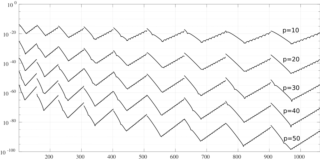
(a)

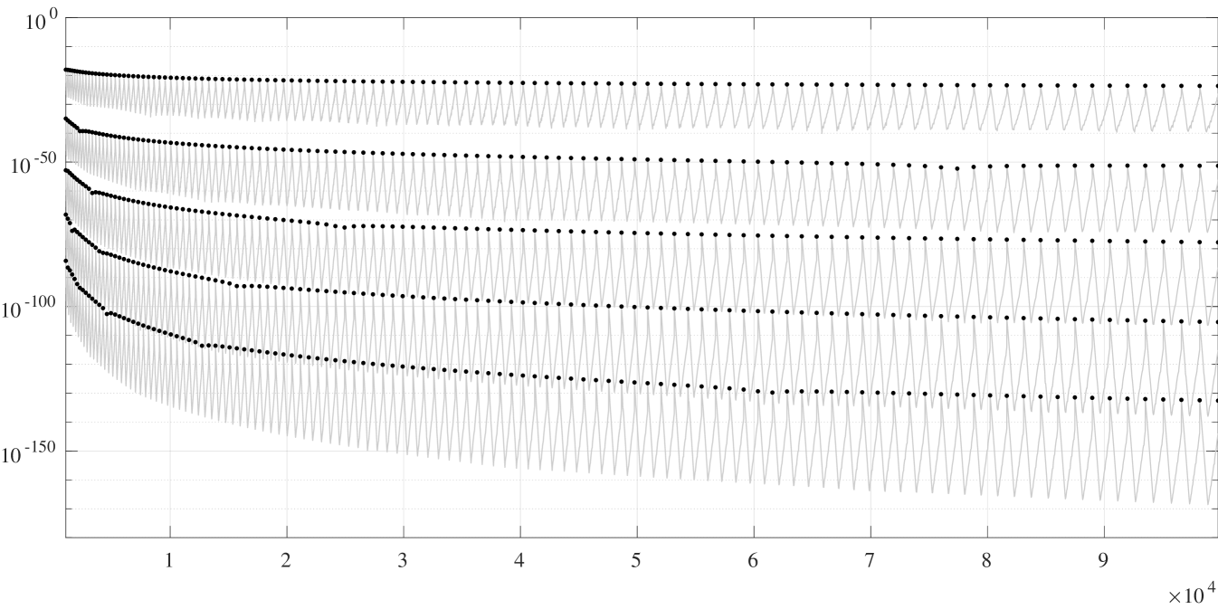
(b)

Figure 2: The values of $\Delta_{p}(t)$ for $p\in\{10,20,30,40,50\}$. The black dots on plot (b) correspond to values of $\Delta_{p}(t_{n})$.

As the first test, we examined the accuracy of the approximations $\zeta_{p}(s)$ in the critical strip. We define $t_{n}:=2\pi n^{2}$, which represents the values of $t$ where $N_{t}=\lfloor\sqrt{t/(2\pi)}\rfloor$ increases by one. Figure 2 displays graphs of $\Delta_{p}(t)$ over two ranges $t_{4}\leq t\leq t_{13}$ (Figure 2a) and $t_{13}\leq t\leq t_{126}$ (Figure 2b), for $p\in\{10,20,30,40,50\}$. We observe that $\Delta_{p}(t)$ exhibits a similar pattern on each interval $[t_{n},t_{n+1}]$: its values tend to be largest near the endpoints of these intervals and smallest near their midpoints. The numerical results presented in Figure 2 suggest that the following error bounds hold for $s=\sigma+{\textnormal{i}}t$ and $0\leq\sigma\leq 1$:

• $|\zeta_{10}(s)-\zeta(s)|<10^{-15}$ when $t>250$ and $|\zeta_{10}(s)-\zeta(s)|<10^{-20}$ when $t>6000$;

• $|\zeta_{20}(s)-\zeta(s)|<10^{-30}$ when $t>350$ and $|\zeta_{20}(s)-\zeta(s)|<10^{-50}$ when $t>65000$;

• $|\zeta_{50}(s)-\zeta(s)|<10^{-100}$ when $t>4000$;

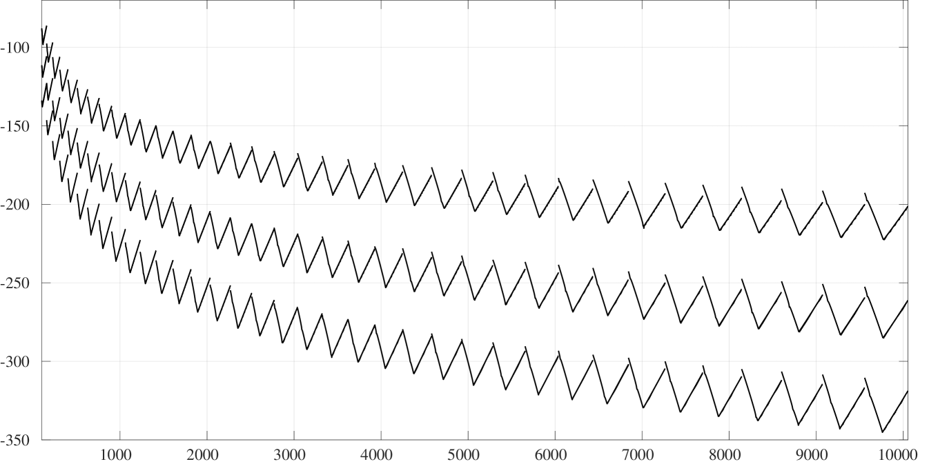
Figure 3: The values of $\log_{10}(\Delta_{p}(t))$ for $p\in\{90,120,150\}$.

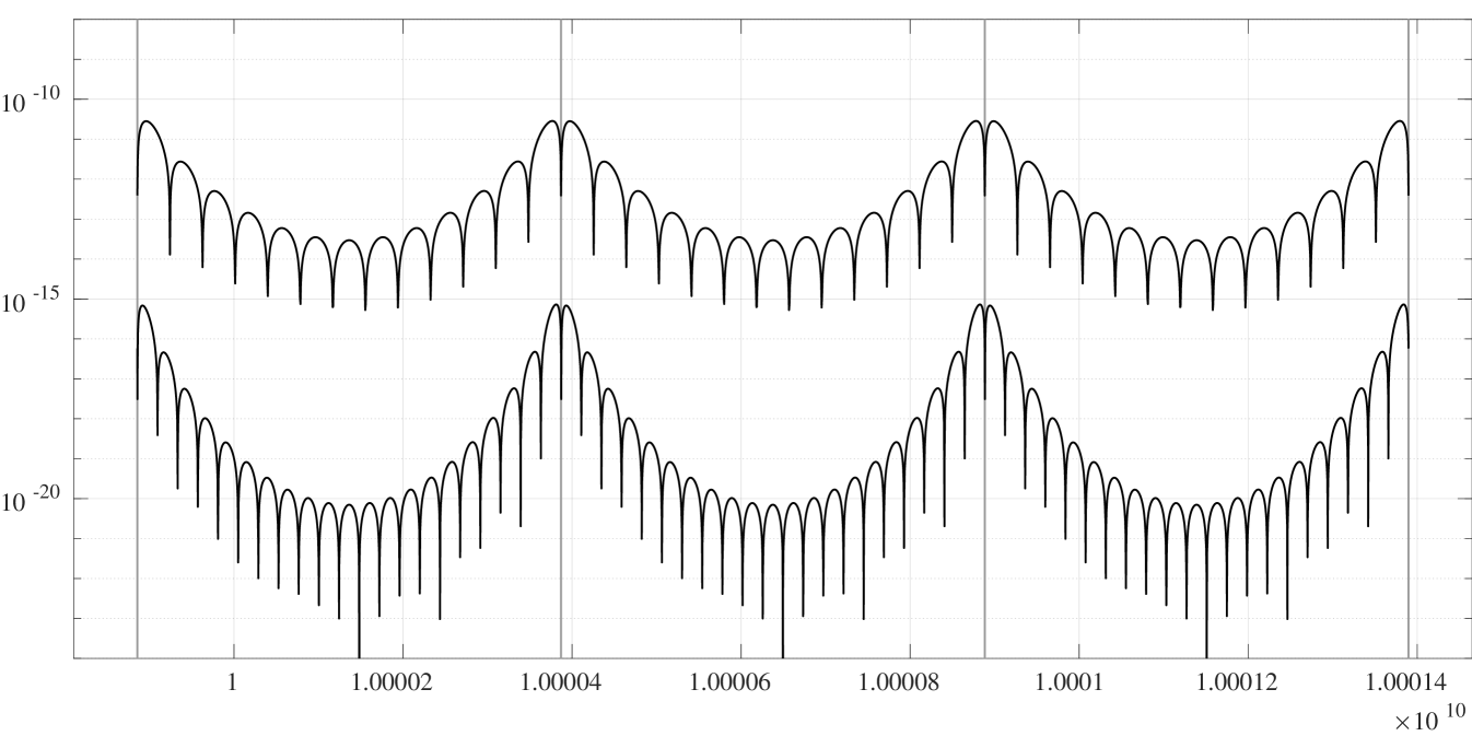
Figure 4: The values of $|\zeta(1/2+{\textnormal{i}}t)-\zeta_{p}(1/2+{\textnormal{i}}t)|$ for $p\in\{3,5\}$ and $t$ close to $10^{10}$. The gray vertical lines show the locations of $t_{n}=2\pi n^{2}$ for $39894\leq n\leq 39897$.

On Figure 3, we plot $\Delta_{p}(t)$ for $p\in\{90,120,150\}$ over the range $t_{4}\leq t\leq t_{40}$. We observe that the error $|\zeta_{p}(s)-\zeta(s)|$ decreases significantly as $p$ increases. These numerical results suggest that for $0\leq\sigma\leq 1$, the following error bounds hold:

• $|\zeta_{120}(s)-\zeta(s)|<10^{-200}$ when $t>1650$;

• $|\zeta_{150}(s)-\zeta(s)|<10^{-300}$ when $t>6900$.

Next, we examine the accuracy of our approximations for very large values of $t$. On Figure 4 we plot the values of $|\zeta_{p}(1/2+{\textnormal{i}}t)-\zeta(1/2+{\textnormal{i}}t)|$ for $p\in\{3,5\}$ and $t$ near $10^{10}$. Again, we observe that these approximations are highly accurate: for these values of $t$, we find $|\zeta_{3}(1/2+{\textnormal{i}}t)-\zeta(1/2+{\textnormal{i}}t)|\leq 10^{-10}$ and the corresponding errors for $\zeta_{5}$ are smaller than $10^{-15}$. Interestingly, these errors exhibit certain patterns: within each interval $t\in[t_{n},t_{n+1}]$, the error $|\zeta_{3}(1/2+{\textnormal{i}}t)-\zeta(1/2+{\textnormal{i}}t)|$ is very small at the endpoints of the interval and also at 12 equally spaced points inside it. A similar pattern holds true for $|\zeta_{5}(1/2+{\textnormal{i}}t)-\zeta(1/2+{\textnormal{i}}t)|$, but with 20 points equally spaced inside each interval. This not a coincidence: in general, for very large $t$, the error $|\zeta_{p}(1/2+{\textnormal{i}}t)-\zeta(1/2+{\textnormal{i}}t)|$ is small at the endpoints of each interval $[t_{n},t_{n+1}]$ and at $4p$ equally spaced points within it. From this pattern, the reader may guess how the coefficients $\omega_{p,j}$ and $\lambda_{p,j}$ were chosen, but we defer this discussion to Section 2.

Computing numerical values of $\zeta^{\prime}(s)$ is also important (see, for example, [11]). Our approximations to $\zeta^{\prime}(s)$ are defined as

$$\zeta^{(1)}_{p}(s):=\frac{\partial}{\partial s}F(s;N,p)\Big{|}_{N=N_{t}},$$

where $F(s;N,p)$ is defined in (3). Note that we can not define $\zeta^{(1)}_{p}(s)$ as $\frac{{\textnormal{d}}}{{\textnormal{d}}s}\zeta_{p}(s)$, as the latter function is not continuous (thus, not differentiable) at $t=t_{n}$. Figure 5 displays graphs of

$$\Delta^{(1)}_{p}(t):=\max\limits_{0\leq k\leq 100}\big{|}\zeta_{p}^{(1)}(\sigma_{k}+{\textnormal{i}}t)-\zeta^{\prime}(\sigma_{k}+{\textnormal{i}}t)\big{|},\;{\textnormal{ where }}\;\sigma_{k}=k/100.$$

The values of $\zeta^{\prime}(s)$ are also computed via Galway’s method [7] (details can be found in Section 2). The graphs on Figure 5 closely resemble those in Figure 2, suggesting that the error $|\zeta^{(1)}_{p}(s)-\zeta^{\prime}(s)|$ is of similar order of magnitude as $|\zeta_{p}(s)-\zeta(s)|$.

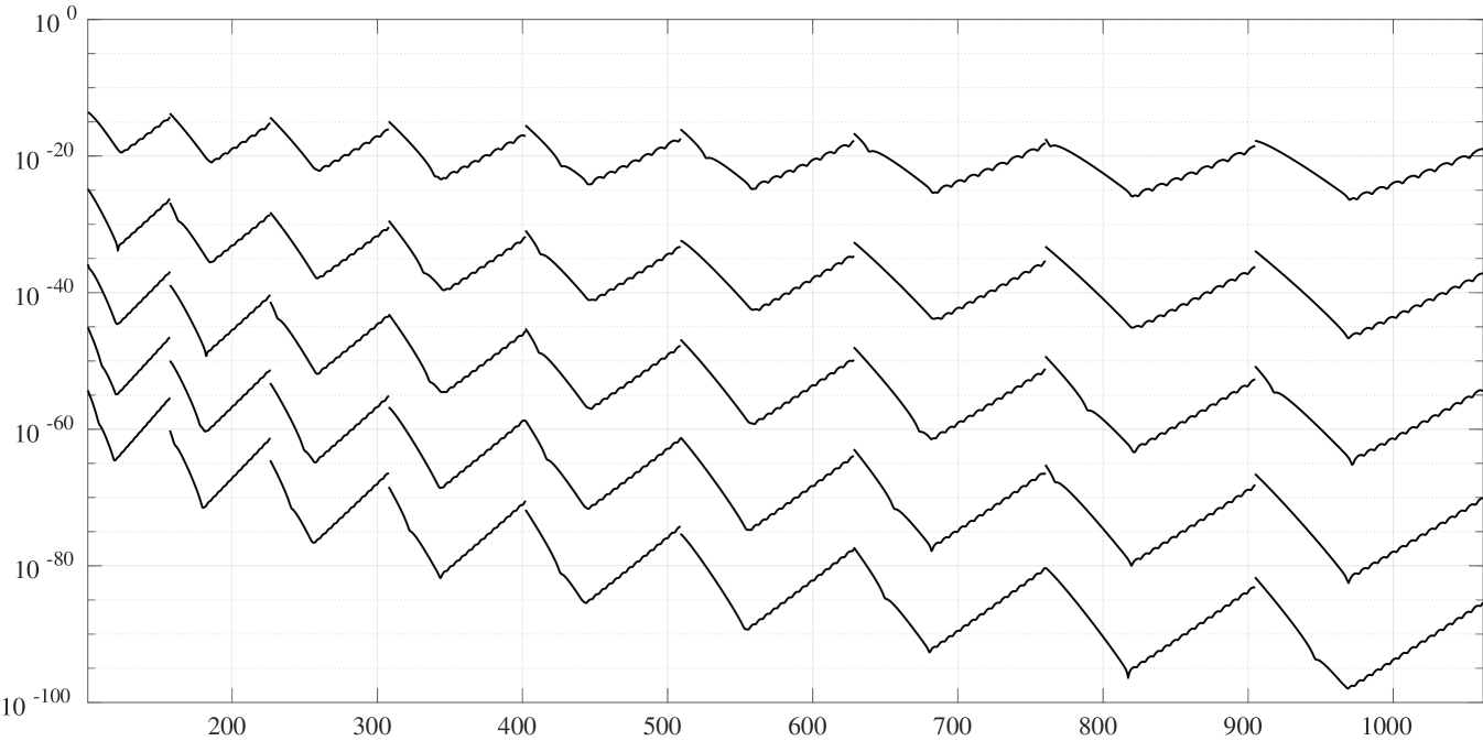
Figure 5: The values of $\Delta^{(1)}_{p}(t)$ for $p\in\{10,20,30,40,50\}$.

The computations in the previous examples were performed with sufficiently high precision to ensure that we could analyze the approximation error $\zeta_{p}(s)-\zeta(s)$ without having to worry about rounding errors. A natural question arises: how accurate are these approximations when implemented in double (or quadruple) precision? To investigate this, we implemented $\zeta_{8}(s)$ and $\zeta_{12}(s)$ in double and quadruple precision, in Fortran90 and MATLAB. The corresponding code can be downloaded at kuznetsov.mathstats.yorku.ca/code/ (see also Appendix B for the MATLAB implementation of $\zeta_{8}(s)$). We tested the accuracy of these approximations in the strip $1/2\leq\textnormal{Re}(s)\leq 2$. This particular strip was chosen because $\zeta(s)$ does not grow too rapidly as $t\to+\infty$ in this strip, unlike in any strip where $\textnormal{Re}(s)<1/2$. The results of these computations are presented in Figure 6.

The top graph shows the error $\Delta_{8}(t;1/2,2)$, where $\zeta_{8}(s)$ was implemented in double precision (the benchmark values $\zeta(s)$ were computed in higher precision). We observe that rounding errors dominate the approximation error for $t>200$. These rounding errors primarily arise when computing $\chi(s)$ and evaluating the values of $n^{-s}$ and $n^{s-1}$ for $s=\sigma+{\textnormal{i}}t$ with even moderatly large $t$. Indeed, it is easy to verify numerically that when computing the value of $2^{{\textnormal{i}}t}$ in double precision for $t$ of the order $10^{2}$, precision of the result will be around $10^{-14}$, and when $t$ increases to $10^{3}$, the precision drops to about $10^{-13}$. This suggests that we lose one decimal digit of precision every time $t$ increases by a factor of ten. Precision is also lost due to cancellation errors when we add many terms in the main sum in (3), though this effect likely plays a lesser role compared to rounding errors.

The middle graph in Figure 6 (shown in gray) displays the errors $\Delta_{8}(t;1/2,2)$, where this time $\zeta_{8}(s)$ was implemented in quadruple precision. We observe that rounding errors do not affect the results in this range of $t$. The quadruple precision implementation of $\zeta_{8}(s)$ produces errors smaller than $10^{-13}$ for $t>250$ and smaller than $10^{-15}$ for $t>2000$ in the strip $1/2\leq\sigma\leq 2$. Of course, when $t$ becomes very large (of the order $10^{10}$ or greater), rounding errors will eventually become noticeable.

The bottom graph on Figure 6 shows the errors $\Delta_{12}(t;1/2,2)$ for the quadruple precision implementation of $\zeta_{12}(s)$. These errors are significantly smaller: we find that $\Delta_{12}(t;1/2,2)<10^{-25}$ for $t>5000$. The effects of rounding errors become clearly noticeable for $t>2000$, though they do not pose a significant issue in this range, as the maximum approximation error remains larger than the rounding errors. However, when $t$ reacher $10^{5}$ or greater, rounding errors will dominate the approximation error, and the graph will resemble the top graph (though with a much smaller overall error, of order $10^{-27}$).

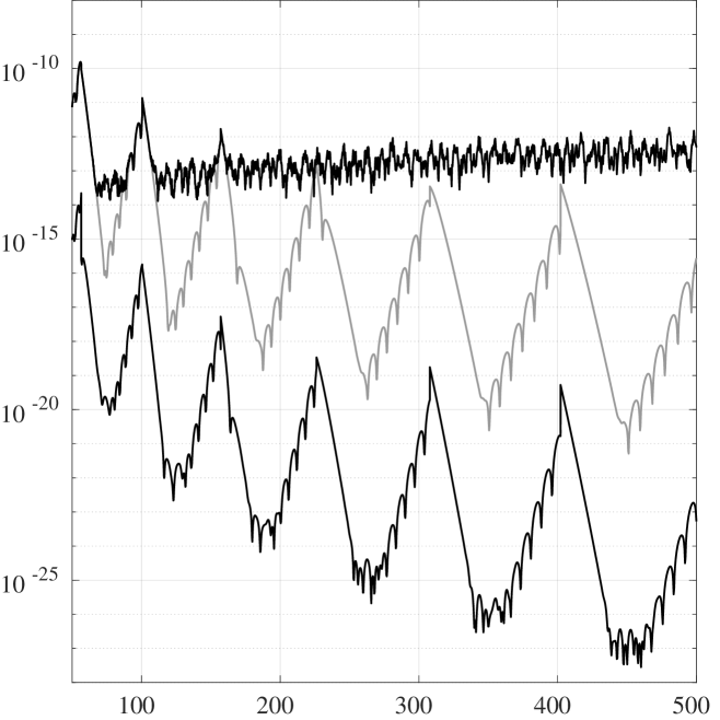
(a)

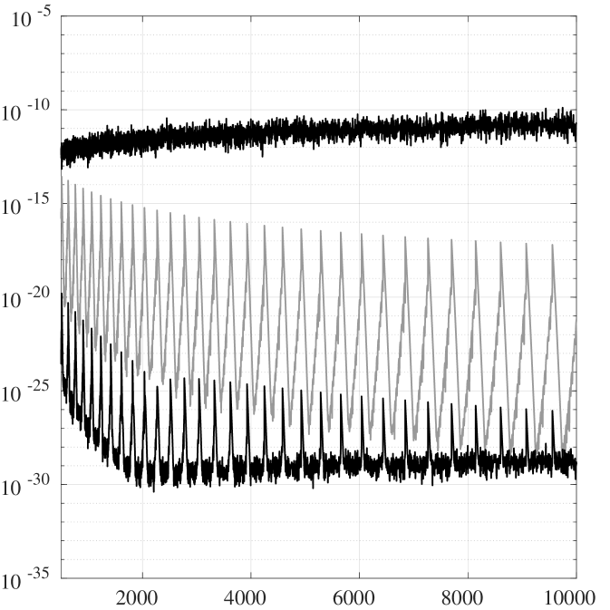
(b)

Figure 6: The values of $\Delta_{p}(t;1/2,2)$. The top curve corresponds to $p=8$ implemented in double precision, the middle curve in gray color (the bottom curve) correspond to $p=8$ and (respectively, $p=12$) impemented in quadruple precision.

Now that we have (hopefully) convinced the reader of the accuracy of our approximations, it is time to discuss how they were derived and to present an algorithm for computing the coefficients $\omega_{p,j}$ and $\lambda_{p,j}$.

2 Deriving the approximations and computing $\omega_{p,j}$ and $\lambda_{p,j}$

We begin with the following result: for every integer $N\geq 0$ and $s\in{\mathbb{C}}$

$$\zeta(s)=\sum\limits_{n=1}^{N}n^{-s}+\chi(s)\sum\limits_{n=1}^{N}n^{s-1}-\frac{(-1)^{N}}{2}\Big{[}{\mathcal{I}}_{N+\frac{1}{2}}(s)+\chi(s)\overline{{\mathcal{I}}}_{N+\frac{1}{2}}(1-s)\Big{]},$$ (6)

where

$${\mathcal{I}}_{M}(s):=\int_{{\mathbb{R}}}\frac{e^{-\pi x^{2}-2\pi M\theta x}}{\cosh(\pi\theta x)}\Big{(}M+\frac{x}{\theta}\Big{)}^{-s}{\textnormal{d}}x,$$ (7)

and $\theta:=\exp(-\pi{\textnormal{i}}/4)$. The function $\overline{{\mathcal{I}}}_{M}$ is defined via (2). The above result is equivalent to formulas (1.1), (1.3) and (1.4) in [7], after a change of variable of integration $z=N+1/2+\theta x$ in [7][equation (1.1)]. It can also be derived from formulas (1.1) and (3.2) in [5].

Formula (6) was used by Galway [7] to derive numerical quadrature algorithm for computing $\zeta(s)$. We used a special case of Galway’s approximations to compute the benchmark values of $\zeta(s)$ and $\zeta^{\prime}(s)$. We approximate ${\mathcal{I}}_{M}(s)$ by

$${\mathcal{I}}_{M}(s;h):=h\sum\limits_{k\in{\mathbb{Z}}}\frac{e^{-\pi(kh)^{2}-2\pi M\theta kh}}{\cosh(\pi\theta kh)}\Big{(}M+\frac{kh}{\theta}\Big{)}^{-s},$$ (8)

where $h>0$. Note that for $M\geq 1/2$, the integrand in (7) is analytic in a strip $|\textnormal{Im}(x)|<\pi/\sqrt{2}$ and decays very rapidly as $|x|\to\infty$. According to Lemma 2.1 and estimates (2.2) and (2.3) in [7], for any $s\in{\mathbb{C}}$, $M\geq 1/2$ and $c\in(0,\pi/\sqrt{2})$ we have

$${\mathcal{I}}_{M}(s;h)-{\mathcal{I}}_{M}(s)=O\big{(}\exp(-c/h)\big{)},\;\;\;h\to 0^{+}.$$ (9)

This result also follows from [24][Theorem 5.1]. The implied constant in the big-O term depends on $s$ and $M$.

We define for $N\geq 0$

$$G(s;N,h):=\sum\limits_{n=1}^{N}n^{-s}+\chi(s)\sum\limits_{n=1}^{N}n^{s-1}-\frac{(-1)^{N}}{2}\Big{[}{\mathcal{I}}_{N+\frac{1}{2}}(s;h)+\chi(s)\overline{{\mathcal{I}}}_{N+\frac{1}{2}}(1-s;h)\Big{]}.$$

Formula (9) implies that for any non-negative integer $N$ we have $G(s;N,h)\to\zeta(s)$ as $h\to 0^{+}$, so that we have an infinite family of approximations to $\zeta(s)$, allowing us to choose (for every $s$) the one that is easiest to compute. It is well known [7, 23] that the optimal choice is $N=N_{t}=\lfloor\sqrt{t/(2\pi)}\rfloor$ (recall that $s=\sigma+{\textnormal{i}}t$ and $t>0$). This choice ensures that the saddle point of the integrand in (7) is as close as possible to the real line. We define $\zeta(s;h)=G(s;N_{t},h)$. This is how we compute the benchmark values of $\zeta(s)$ to high precision. Galway [7] developed more general (and more efficient) approximations, but this simple version suffices for our purposes. To implement $\zeta(s;h)$, we used Stirling’s series algorithm for computing the Gamma function [13] and truncated the infinite sum in (8) once the terms became smaller than $10^{-d}$, where $d$ is the working precision. To illustrate the accuracy of this approximation, we conducted the following experiment. We downloaded the value of 30th zero $1/2+{\textnormal{i}}\gamma_{30}$ of the Riemann zeta function in the critical strip, which was computed to 1000 decimal digits in [18], and we evaluated $\zeta(1/2+{\textnormal{i}}\gamma_{30};h)$ for a decreasing sequence of $h$. The results, shown on Figure 6, demonstrate that the values of $\zeta(1/2+{\textnormal{i}}\gamma_{30};h)$ decrease precisefly at the rate $\exp(-\frac{\pi}{\sqrt{2}}\times\frac{1}{h})$, which is consistent with (9).

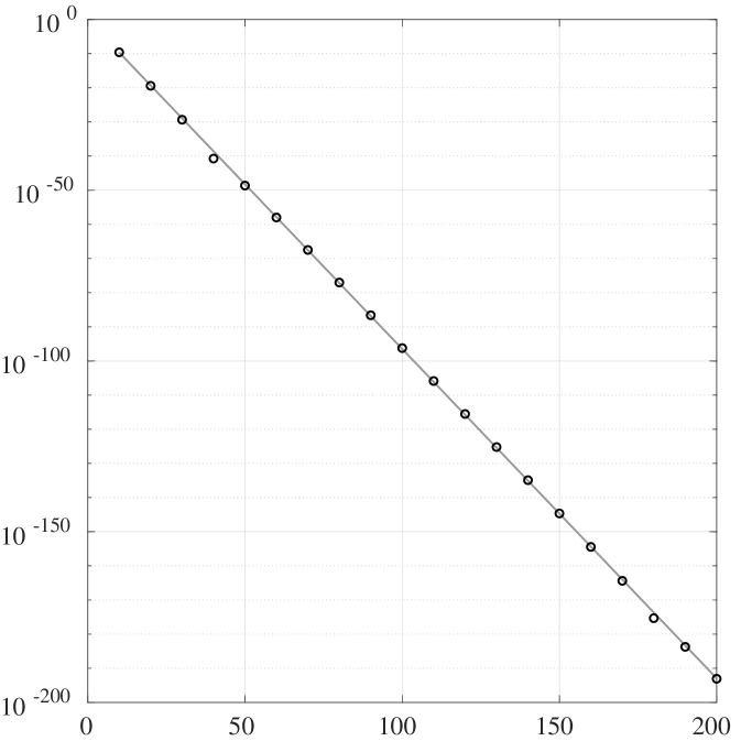
Figure 7: The values of $|\zeta(1/2+{\textnormal{i}}\gamma_{30};h)|$ (circles) and $\exp(-\frac{\pi}{\sqrt{2}}\times\frac{1}{h})$ (gray line), where $\frac{1}{h}$ is on the $x$-axis.

To compute the benchmark values of $\zeta^{\prime}(s)$ (needed for the results on Figure 5), we approximated it using

$$\zeta^{(1)}(s;h):=\frac{\partial}{\partial s}G(s;N;h)\Big{|}_{N=N_{t}}.$$

We also conducted several numerical experiments confirming that $\zeta^{(1)}(s;h)\to\zeta^{\prime}(s)$ as $h\to 0^{+}$ at the same rate $\exp(-\frac{\pi}{\sqrt{2}}\times\frac{1}{h})$.

Now we are ready to introduce the ideas behind our approximations and the method for computing the coefficients $\omega_{p,j}$ and $\lambda_{p,j}$. Formula (6) shows that we can compute $\zeta(s)$ once we we have an effective way to evaluate ${\mathcal{I}}_{M}(s)$. We rewrite (7) in the form

$${\mathcal{I}}_{M}(s):=M^{-s}\int_{{\mathbb{R}}}e^{g(x;s)}\times\frac{e^{-\pi x^{2}}}{\cosh(\pi\theta x)}{\textnormal{d}}x=M^{-s}\int_{{\mathbb{R}}}e^{g(x;s)}\eta({\textnormal{d}}x),$$ (10)

where we denoted

$$g(x)=g(x;s):=-2M\pi\theta x-s\ln\Big{(}1+\frac{x}{M\theta}\Big{)}\;\;\;\;{\textnormal{ and }}\;\;\;\;\eta({\textnormal{d}}x):=\frac{e^{-\pi x^{2}}}{\cosh(\pi\theta x)}{\textnormal{d}}x.$$

We consider the numbers $\omega_{p,j}$ and $x_{p,j}=\lambda_{p,j}/\theta$ as the weights and nodes of a discrete measure

$$\eta_{p}({\textnormal{d}}x)=\omega_{p,0}\delta_{0}({\textnormal{d}}x)+\sum\limits_{j=1}^{p}\omega_{p,j}\Big{[}\delta_{x_{p,j}}({\textnormal{d}}x)+\delta_{-x_{p,j}}({\textnormal{d}}x)\Big{]},$$

which serves as an approximation to $\eta({\textnormal{d}}x)$. Approximating $\eta({\textnormal{d}}x)$ by $\eta_{p}({\textnormal{d}}x)$ provides an approximation for the corresponding integrals

$$\int_{{\mathbb{R}}}f(x)\eta({\textnormal{d}}x)\approx\int_{{\mathbb{R}}}f(x)\eta_{p}({\textnormal{d}}x)=\omega_{p,0}f(0)+\sum\limits_{j=1}^{p}\omega_{p,j}\Big{[}f(x_{p,j})+f(-x_{p,j})\big{]}.$$ (11)

A classical way for determining the coefficients $\omega_{p,j}$ and $x_{p,j}$ is to require that (11) holds exactly for a chosen set of functions $f_{k}(x)$. For example, the Gaussian quadrature method requires (19) to be exact for all polynomials of degree $\leq 4p+1$. In fact, this was the first approach we explored, and while it produces decent results, the method we introduce next provides better accuracy and is somewhat easier to implement.

For the remainder of this section, we assume that $s$ lies within a fixed vertical strip $a\leq\sigma\leq b$ and we set $M=N_{t}+1/2$, where $s=\sigma+{\textnormal{i}}t$, $t>0$ and $N_{t}=\lfloor\sqrt{t/(2\pi)}\rfloor$. We now examine the asymptotic behavior of the integrand in (10). Expanding $g(x;s)$ in Taylor series around $x=0$, we obtain

$$g(x;s)=\Big{(}-\frac{{\textnormal{i}}s}{2\pi M}-M\Big{)}2\pi\theta x+\frac{1}{2}\frac{s}{M^{2}\theta^{2}}x^{2}+\sum\limits_{k\geq 3}\frac{(-1)^{k}}{k}\frac{s}{M^{k}\theta^{k}}x^{k},\;\;\;|x|<M.$$ (12)

The first coefficient in this expansion simplifies to

$$-\frac{{\textnormal{i}}s}{2\pi M}-M=\frac{t-{\textnormal{i}}\sigma}{2\pi(N_{t}+\frac{1}{2})}-N_{t}-\frac{1}{2}=\frac{t}{2\pi N_{t}}-N_{t}-1+O(t^{-1/2}),$$

as $t\to+\infty$. Defining

$$B(t):=\frac{t}{2\pi N_{t}}-N_{t}-1.$$

and using the inequality $N_{t}\leq\sqrt{t/(2\pi)}<N_{t}+1$, we obtain the bound

$$-1\leq B(t)\leq 1+O(t^{-1/2}).$$ (13)

The second coefficient in (12) simplifies to

$$\frac{1}{2}\frac{s}{M^{2}\theta^{2}}=-\frac{t}{2(N_{t}+\frac{1}{2})^{2}}+O(t^{-1})=-\pi+O(t^{-1/2}).$$

When $t$ is large enough, we have $|s|<2t$ and $M=N_{t}+1/2>\sqrt{t}/3$ (since $\sqrt{2\pi}<3$). Therefore, for $t$ large enough, the sum in (12) can be estimated as follows

$$\Big{|}\sum\limits_{k\geq 3}\frac{(-1)^{k}}{k}\frac{s}{M^{k}\theta^{k}}x^{k}\Big{|}<2t\sum\limits_{k\geq 3}\Big{(}3|x|/\sqrt{t}\Big{)}^{k}=\frac{54|x|^{3}}{\sqrt{t}-3|x|},$$ (14)

for $|x|<\sqrt{t}/3$. Thus, we conclude that

$$g(x;s)=-\pi x^{2}+2\pi\theta B(t)x+O(t^{-1/2}),$$ (15)

as $t\to+\infty$, uniformly in $x$ on compact subsets of ${\mathbb{C}}$.

For $t$ large, the integral in (10) is therefore approximately equal to

$$\int_{{\mathbb{R}}}e^{-\pi x^{2}+2\pi\theta B(t)x}\eta({\textnormal{d}}x),$$

where $B(t)$ typically lies in the interval $[-1,1]$, though occasionally it may slightly exceed one (see figure 8).

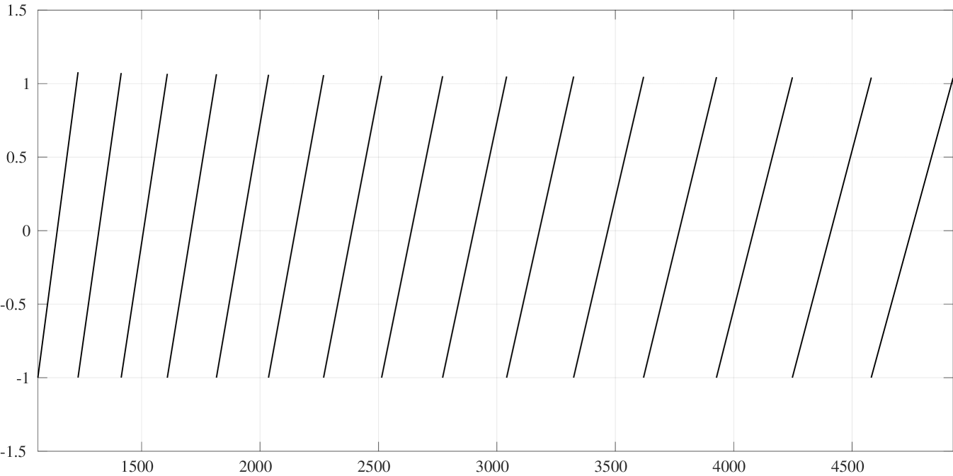
Figure 8: The graph of $B(t)$.

To determine the quadrature coefficients $\{\omega_{p,j}\}_{0\leq j\leq p}$ and $\{x_{p,j}\}_{1\leq j\leq p}$, we require that (11) holds exactly for a set of $4p+2$ functions

$$f_{k}(x)=e^{-\pi x^{2}+2\pi\theta y_{k}x},\;\;\;k=0,1,\dots,4p+1,$$

where the points $\{y_{k}\}_{0\leq k\leq 4p+1}$ are equally spaced in the interval $[-1,1]$:

$$y_{k}:=-1+\frac{2k}{4p+1}.$$

Thus, we arrive at the following problem: we seek $2p+1$ complex numbers $\{\omega_{p,j}\}_{0\leq j\leq p}$ and $\{x_{p,j}\}_{1\leq j\leq p}$ such that

$$\int_{{\mathbb{R}}}\frac{e^{-2\pi x^{2}+2\pi\theta y_{k}x}}{\cosh(\pi\theta x)}{\textnormal{d}}x=\omega_{p,0}+\sum\limits_{j=1}^{p}\omega_{p,j}e^{-\pi x_{p,j}^{2}}\Big{[}e^{2\pi\theta y_{k}x_{p,j}}+e^{-2\pi\theta y_{k}x_{p,j}}\big{]},$$ (16)

for all $k=0,1,\dots,4p+1$.

To simplify the above problem, we note that the integral on the left-hand side of (16) is one of Mordell integrals [17] and can be computed explicitly. Using formula (7) in [14] (or transforming the integral in [6][Theorem 4.1.1]) we evaluate

$$H(y):=\int\limits_{{\mathbb{R}}}\frac{e^{-2\pi x^{2}+2\pi\theta xy}}{\cosh(\pi\theta x)}{\textnormal{d}}x=\frac{1}{\cos(\pi y)}\Big{[}\sqrt{2}\cos(\pi y/2)e^{-\frac{\pi{\textnormal{i}}}{8}(4y^{2}+1)}-e^{-\frac{\pi{\textnormal{i}}}{4}}\Big{]}.$$ (17)

We denote $\mu_{k}:=H(y_{k})$ and introduce new variables $\{u_{j},z_{j}\}_{-p\leq j\leq p}$, defined as follows: $u_{0}=w_{p,0}$, $z_{0}=1$ and for $j=1,2,\dots,p$

$$u_{j}:=\omega_{p,j}e^{-\pi x_{p,j}^{2}-2\pi\theta x_{p,j}},\;\;\;u_{-j}:=\omega_{p,j}e^{-\pi x_{p,j}^{2}+2\pi\theta x_{p,j}},\;\;\;z_{j}:=e^{2\pi\theta\frac{2}{4p+1}x_{p,j}},\;\;\;z_{-j}:=1/z_{j}.$$ (18)

In these new variables, the system of equations (16) simplifies to

$$\sum\limits_{j=-p}^{p}u_{j}z_{j}^{k}=\mu_{k},\;\;\;k=0,1,\dots,4p+1.$$ (19)

Our task is now to determine the values of $\{u_{j},z_{j}\}_{-p\leq j\leq p}$ satisfying $z_{0}=1$, $z_{-j}=1/z_{j}$ and $u_{-j}=z_{j}^{4p+1}u_{j}$ for $j=1,2,\dots,p$, which solve the system of equations (19).

The solution to the above system of equations is obtained using classical methods of Gaussian quadrature [16]. Let $\mathcal{P}_{n}$ be the space of polynomials with complex coefficients of degree not exceeding $n$. Define a linear functional $L$ acting on $\mathcal{P}_{4p+1}$ via

$$L[x^{k}]=\mu_{k},\;\;\;k=0,1,\dots,4p+1.$$

The system (19) is equivalent to the condition

$$L[Q]=\sum\limits_{j=-p}^{p}u_{j}Q(z_{j})\;\;{\textnormal{ for all }}\;Q\in\mathcal{P}_{4p+1}.$$ (20)

To obtain a solution to (20), we first compute monic orthogonal polynomials $\{P_{n}(x)\}_{0\leq n\leq m}$ (where $m:=2p+1$), satisfying the orthogonality condition with respect to $L$: for $1\leq n\leq m$

$$L[P_{n}Q]=0\;{\textnormal{ for all }}\;Q\in\mathcal{P}_{n-1}.$$

The polynomials $\{P_{n}(x)\}_{0\leq n\leq m}$ are computed via the three-term recurrence relation

$$P_{n+1}(x)=(x-a_{n})P_{n}(x)-b_{n}P_{n-1}(x),\;\;\;n=0,1,\dots m-1,$$ (21)

with initial conditions $P_{-1}(x)\equiv 0$, $P_{0}(x)\equiv 1$. The recurrence coefficients are given by

$$a_{n}=\frac{L[xP_{n}^{2}]}{L[P_{n}^{2}]},\;\;\;b_{n}=\frac{L[P_{n}^{2}]}{L[P_{n-1}^{2}]}.$$

The existence of orthogonal polynomials $\{P_{n}(x)\}_{0\leq n\leq m}$ is not guaranteed, as the functional $L$ does not come from integration with respect to a positive measure. Thus, in principle, it is possible that $L[P_{n}^{2}]=0$ for some $n$. However, in practice, we never encountered this issue when computing these polynomials. For now, we assume that we are able to compute orthogonal polynomials $\{P_{n}(x)\}_{0\leq n\leq m}$.

Before we proceed, we establish the following result:

Proposition 1.

The polynomial $P_{m}$ satisfies $P_{m}(x)=-x^{m}P_{m}(1/x)$ for all $x\neq 0$.

Proof.

We begin by stating a preliminary result about determinants. Let $B=\{b_{i,j}\}_{1\leq i,j\leq n}$ be $n\times n$ matrix. Following [8], we denote by $B^{\tau}$ the transpose of $B$ with respect to anti-diagonal. In other words, $B^{\tau}=\{\tilde{b}_{i,j}\}_{1\leq i,j\leq n}$ where $\tilde{b}_{i,j}=b_{n+1-j,n+1-i}$ for $1\leq i,j\leq n$. It is true that

$${\textnormal{det}}(B)={\textnormal{det}}(B^{\tau}).$$ (22)

This follows from the factorization $B^{\tau}={\textrm{J}}B^{T}{\textrm{J}}$ (see [8]), where J is $n\times n$ matrix with ${\textrm{J}}_{i,j}=1$ if $i+j=n+1$ and ${\textrm{J}}_{i,j}=0$ otherwise.

Now we can prove Proposition 1. Since $H(y)$ is an even function (see (17)), the numbers $\mu_{k}=H(y_{k})$ satisfy $\mu_{k}=\mu_{4p+1-k}$ for $0\leq k\leq 4p+1$. Using this fact and the well-known representation of orthogonal polynomials as determinants, we obtain

$$P_{m}(x)=C\times{\textnormal{det}}\begin{bmatrix}\mu_{0}&\mu_{1}&\mu_{2}&\cdots&\mu_{2p-1}&\mu_{2p}&\mu_{2p}\\ \mu_{1}&\mu_{2}&\mu_{3}&\cdots&\mu_{2p}&\mu_{2p}&\mu_{2p-1}\\ \mu_{2}&\mu_{3}&\mu_{4}&\cdots&\mu_{2p}&\mu_{2p-1}&\mu_{2p-2}\\ \cdots&\cdots&\cdots&\cdots&\cdots&\cdots&\cdots\\ \mu_{2p-1}&\mu_{2p}&\mu_{2p}&\cdots&\mu_{3}&\mu_{2}&\mu_{1}\\ \mu_{2p}&\mu_{2p}&\mu_{2p-1}&\cdots&\mu_{2}&\mu_{1}&\mu_{0}\\ 1&x&x^{2}&\cdots&x^{2p-1}&x^{2p}&x^{2p+1}\end{bmatrix}$$ (23)

for some constant $C$. For $k=0,1,\dots,m$ we denote by $A_{k}$ the submatrix obtained from the matrix in (23) by removing the last row and $(k+1)$-st column. Performing Laplace expansion along the last row, we obtain

$$P_{m}(x)=C\sum\limits_{k=0}^{m}(-1)^{k}{\textnormal{det}}(A_{k})x^{k}.$$

It is straighforwad to verify that $A_{k}=A_{m-k}^{\tau}$. The desired result follows from (22). $\sqcap\kern-8.0pt\hbox{$\sqcup$}$

We assume that all roots $\{z_{j}\}_{-p\leq j\leq p}$ of the polynomial $P_{m}$ are simple. While this would be guaranteed if the numbers $\mu_{k}$ were moments of a positive measure (which is not the case here), in all our computations we found that the roots $P_{m}$ were indeed simple. Proposition 1 implies that one of the roots must be equal to $1$ and the other roots come in pairs $z_{j}$ and $1/z_{j}$. This allows us to order the roots $\{z_{j}\}_{-p\leq j\leq p}$ in increasing order of their absolute values (that is, $|z_{j}|\leq|z_{j+1}|$) and in such a way that $z_{-j}=1/z_{j}$ and $z_{0}=1$. The weights of the Gaussian quadrature are computed using [16][formula (3)]:

$$u_{j}=\frac{L[P_{m-1}^{2}]}{P_{m-1}(z_{j})P_{m}^{\prime}(z_{j})},\;\;\;-p\leq j\leq p.$$ (24)

Note that $P_{m}^{\prime}(z_{j})\neq 0$ due to our assumption that the roots are simple. Additionally, $P_{m-1}(z_{j})\neq 0$, since otherwise, the three-term recurrence (21) would imply that $P_{n}(z_{j})=0$ for all $0\leq n\leq m$, which is impossible (recall that $P_{0}(z)\equiv 1$).

We claim that the weights and nodes of this Gaussian quadrature satisfy the identity $u_{-j}=z_{j}^{4p+1}u_{j}$. This follows from (19) and the symmetry relation $\mu_{k}=\mu_{4p+1-k}$. Indeed, after we found $z_{j}$ and established that $z_{-j}=1/z_{j}$, we can interpret (19) as a system of linear equations in the $2p+1$ unknowns $\{u_{j}\}_{-p\leq j\leq p}$. This system has a unique solution, since its coefficient matrix is the Vandermonde matrix constructed from distinct numbers $\{z_{j}\}_{-p\leq j\leq p}$. By changing indices $k\to 4p+1-k$ and $j\mapsto-j$ in (19), and using the identities $\mu_{k}=\mu_{4p+1-k}$ and $1/z_{j}=z_{-j}$, we conclude that the numbers $\{u_{-j}z_{j}^{-4p-1}\}_{-p\leq j\leq p}$ also solve the same system of equations. By the uniqueness of the solution, it follows that $u_{-j}=u_{j}z_{j}^{4p+1}$ for all $-p\leq j\leq p$.

After we found the nodes $\{z_{j}\}_{-p\leq j\leq p}$ and the weights $\{u_{j}\}_{-p\leq j\leq p}$ of Gaussian quadrature (20), we compute $\omega_{p,j}$ and $x_{p,j}$ from (25). We set $\omega_{p,0}=u_{0}$ and

$$x_{p,j}=\frac{4p+1}{4\pi\theta}\log(z_{j}),\;\;\;\omega_{p,j}=u_{j}e^{\pi x_{j}^{2}+2\pi\theta x_{j}},\;\;\;j=1,2,\dots,p.$$ (25)

By construction, these numbers $\{\omega_{p,j}\}_{0\leq j\leq p}$ and $\{x_{p,j}\}_{1\leq j\leq p}$ must satisfy the system of equations (16).

With the coefficients $\{\omega_{p,j}\}_{0\leq j\leq p}$ and $\{x_{p,j}\}_{1\leq j\leq p}$ computed, we can now use (11) and approximate

$${\mathcal{I}}_{M}(s) =\int_{{\mathbb{R}}}\frac{e^{-\pi x^{2}-2\pi M\theta x}}{\cosh(\pi\theta x)}\Big{(}M+\frac{x}{\theta}\Big{)}^{-s}{\textnormal{d}}x$$

$$\approx\omega_{p,0}M^{-s}+\sum\limits_{j=1}^{p}\omega_{p,j}\Big{[}e^{-2\pi M\theta x_{p,j}}\Big{(}M+\frac{x_{p,j}}{\theta}\Big{)}^{-s}+e^{2\pi M\theta x_{p,j}}\Big{(}M-\frac{x_{p,j}}{\theta}\Big{)}^{-s}\Big{]}.$$

We recognize that the right-hand side is precisely ${\mathcal{I}}_{M,p}(s)$ defined in (1) (recall that we denoted $\theta x_{p,j}=\lambda_{p,j}$).

It remains to explain the pattern in the error $\zeta_{p}(1/2+{\textnormal{i}}t)-\zeta(1/2+{\textnormal{i}}t)$ that we observed on Figure 4. Define the function

$$H_{p}(y):=\omega_{p,0}+2\sum\limits_{j=1}^{p}\omega_{p,j}e^{-\pi{\textnormal{i}}\lambda_{p,j}^{2}}\cosh(2\pi\lambda_{p,j}y).$$ (26)

The system of equations (16) is equivalent to

$$H_{p}(y_{k})=H(y_{k}),\;\;\;k=0,1,\dots,4p+1,$$ (27)

where we recall that $y_{k}=-1+2k/(4p+1)$ and $H(y)$ is defined in (17). We remark here that equations (27) are particularly useful: they allowed us to verify the accuracy of the computed values of $\{\omega_{p,j}\}_{0\leq j\leq p}$ and $\{\lambda_{p,j}\}_{1\leq j\leq p}$. To proceed, we interpret $H_{p}(y)$ as an approximation to the Mordell integral $H(y)$: this approximation is exact at $4p+2$ equally spaced points on $[-1,1]$. On Figure 9, we plot the error $|H_{p}(y)-H(y)|$ of this approximation for $p=3$ and $p=5$. These graphs closely resemble those in Figure 4, which display the error $|\zeta(1/2+{\textnormal{i}}t)-\zeta_{p}(1/2+{\textnormal{i}}t)|$ for $p\in\{3,5\}$ at large values of $t$. Let us now explore the reason for this resemblance.

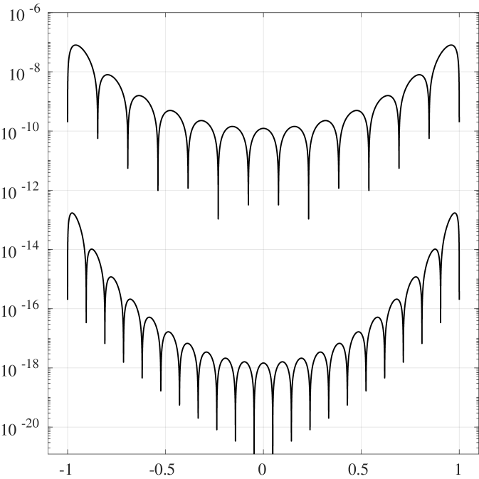
Figure 9: The values of $|H_{p}(y)-H(y)|$ for $-1\leq y\leq 1$ and $p\in\{3,5\}$.

We rewrite (10) in an equivalent form:

$${\mathcal{I}}_{M}(s)=M^{-s}\int_{{\mathbb{R}}}\frac{e^{-2\pi x^{2}+2\pi\theta B(t)x}}{\cosh(\pi\theta x)}{\textnormal{d}}x+M^{-s}\int_{{\mathbb{R}}}\frac{e^{-2\pi x^{2}+2\pi\theta B(t)x}}{\cosh(\pi\theta x)}\times\Big{[}e^{\pi x^{2}-2\pi\theta B(t)x+g(x;s)}-1\Big{]}{\textnormal{d}}x.$$

According to (15), the term inside the square brackets converges to zero as $t\to+\infty$. From the Dominated Convergence Theoerem, the second integral in the right-hand side is $o(1)$ as $t\to+\infty$. Thus we obtain

$${\mathcal{I}}_{M}(s)=M^{-s}H(B(t))+o(M^{-s}),\;\;\;t\to+\infty.$$

From (1) and (15), we find that as $t\to+\infty$

$$M^{s}{\mathcal{I}}_{M,p}(s) =\omega_{p,0}+\sum\limits_{j=1}^{p}\omega_{p,j}\Big{[}e^{g(\lambda_{p,j}/\theta;s)}+e^{g(-\lambda_{p,j}/\theta;s)}\Big{]}$$

$$\longrightarrow\omega_{p,0}+\sum\limits_{j=1}^{p}\omega_{p,j}\Big{[}e^{-\pi{\textnormal{i}}\lambda_{p,j}^{2}+2\pi B(t)\lambda_{p,j}}+e^{-\pi{\textnormal{i}}\lambda_{p,j}^{2}-2\pi B(t)\lambda_{p,j}}\Big{]}=H_{p}(B(t)).$$

From these results, it follows that

$${\mathcal{I}}_{M,p}(s)-{\mathcal{I}}_{M}(s)=M^{-s}\times\big{(}H_{p}(B(t))-H(B(t))\big{)}+o(M^{-s}),\;\;\;t\to+\infty,$$ (28)

which implies

$$\overline{{\mathcal{I}}}_{M,p}(1-s)-\overline{{\mathcal{I}}}_{M}(1-s)=M^{s-1}\times\big{(}\overline{H}_{p}(B(t))-\overline{H}(B(t))\big{)}+o(M^{s-1}),\;\;\;t\to+\infty.$$ (29)

Using (4) and Stirling’s asymptotic formula for the Gamma function, we obtain

$$\chi(s)=M^{1-2s}\times e^{\frac{\pi{\textnormal{i}}}{4}+{\textnormal{i}}t}\Big{(}\frac{t}{2\pi M^{2}}\Big{)}^{\frac{1}{2}-s}\times\big{(}1+O(t^{-1})\big{)}.$$

Denote $\tau:=2(\sqrt{t/(2\pi)}-M)$. Writing

$$\ln\Big{(}\frac{t}{2\pi M^{2}}\Big{)}=\ln\Big{(}1+\frac{t-2\pi M^{2}}{2\pi M^{2}}\Big{)}=\ln\Big{(}1+\tau\frac{\sqrt{t/(2\pi)}+M}{2M^{2}}\Big{)},$$

expanding the logarithm in Taylor series and simplifying the result, we obtain

$$\chi(s)=M^{1-2s}\times e^{\frac{3\pi{\textnormal{i}}}{4}-\pi{\textnormal{i}}\tau^{2}}\times\Big{(}1+O\big{(}t^{-\frac{1}{2}}\big{)}\Big{)}.$$

Combining all the above result with (5), (6), (28) and (29) we arrive at

$$\zeta_{p}(s)-\zeta(s)=-\frac{(-1)^{N}}{2}M^{-s}\Big{[}\big{(}H_{p}(B(t))-H(B(t))\big{)}+e^{\frac{3\pi{\textnormal{i}}}{4}-\pi{\textnormal{i}}\tau^{2}}\times\big{(}\overline{H}_{p}(B(t))-\overline{H}(B(t))\big{)}\Big{]}+o(M^{-s}).$$

Thus we see that the dominant term in the error $\zeta_{p}(s)-\zeta(s)$ vanishes when $B(t)=y_{k}$. This explains the behaviour of the error on Figure 4: when $n$ is large, the error $\zeta_{p}(s)-\zeta(s)$ is small at $4p+2$ equally spaced points within the interval $[t_{n},t_{n+1}]$ because the dominant asymptotic term is zero at those points.

Appendix A     The coefficients $\omega_{p,j}$ and $\lambda_{p,j}$ for $p\in\{5,10\}$

High-precision values of coefficients $\{\omega_{p,j}\}_{0\leq j\leq p}$ and $\{\lambda_{p,j}\}_{1\leq j\leq p}$ for $p=1,2,\dots,30$ and for many values in the range $p\leq 150$ can be downloaded from kuznetsov.mathstats.yorku.ca/code/

$$\omega_{5,0} =2.354383173482941501\text{\text{e-}}1+{\textnormal{i}}\times 3.295537698903362209\text{\text{e-}}2,$$

$$\omega_{5,1} =1.737747054311600606\text{e-}1+{\textnormal{i}}\times 5.726284240637533629\text{e-}2,$$

$$\omega_{5,2} =5.708483151712981717\text{e-}2+{\textnormal{i}}\times 5.367826163392843596\text{e-}2,$$

$$\omega_{5,3} =5.455260017239278090\text{e-}3+{\textnormal{i}}\times 1.692893836426674071\text{e-}2,$$

$$\omega_{5,4} =-4.138943380524367182\text{e-}4+{\textnormal{i}}\times 2.034356935140766843\text{e-}3,$$

$$\omega_{5,5} =-6.653714335968984044\text{e-}5+{\textnormal{i}}\times 6.462574635932469471\text{e-}5$$

$$\lambda_{5,1} =1.881852180702220422\text{e-}1-{\textnormal{i}}\times 1.449755745395875068\text{e-}1,$$

$$\lambda_{5,2} =3.717705006684543749\text{e-}1-{\textnormal{i}}\times 3.020416160270775712\text{e-}1,$$

$$\lambda_{5,3} =5.604567753443639984\text{e-}1-{\textnormal{i}}\times 4.801938441334826040\text{e-}1,$$

$$\lambda_{5,4} =7.672689586414600920\text{e-}1-{\textnormal{i}}\times 6.821905910209796031\text{e-}1,$$

$$\lambda_{5,5} =1.010783983564685329-{\textnormal{i}}\times 9.231734623461863512\text{e-}1.$$

$$\omega_{10,0} =1.746071737157674980979293520809\text{e-}1+{\textnormal{i}}\times 2.131147093009280730611467019158\text{e-}2,$$

$$\omega_{10,1} =1.490803915553910597329354639778\text{e-}1+{\textnormal{i}}\times 3.499836079601156948133789078972\text{e-}2,$$

$$\omega_{10,2} =8.492465921092508217336004148263\text{e-}2+{\textnormal{i}}\times 4.854991766416009886502556092917\text{e-}2,$$

$$\omega_{10,3} =2.794492162555768303150174880103\text{e-}2+{\textnormal{i}}\times 3.428439466181300925395192520791\text{e-}2,$$

$$\omega_{10,4} =4.612090699061725829646273271703\text{e-}3+{\textnormal{i}}\times 1.373142646307427391022925045066\text{e-}2,$$

$$\omega_{10,5} =-3.895212927973588318860893961158\text{e-}5+{\textnormal{i}}\times 3.550886924259579942806268192521\text{e-}3,$$

$$\omega_{10,6} =-2.151575611923250640729364801406\text{e-}4+{\textnormal{i}}\times 6.084356024918800989143391852680\text{e-}4,$$

$$\omega_{10,7} =-5.199488450834904743451274940186\text{e-}5+{\textnormal{i}}\times 6.406830664562431793000193930144\text{e-}5,$$

$$\omega_{10,8} =-5.856003331642731075366848061989\text{e-}6+{\textnormal{i}}\times 3.353733365341979352981823198386\text{e-}6,$$

$$\omega_{10,9} =-2.945578758160111306783176275407\text{e-}7+{\textnormal{i}}\times 3.154278990732981364449273807939\text{e-}8,$$

$$\omega_{10,10} =-4.219551146037265608639695765718\text{e-}9-{\textnormal{i}}\times 1.752142489214440816303376939714\text{e-}9,$$

$$\lambda_{10,1} =1.379409313309054508271675868217\text{e-}1-{\textnormal{i}}\times 1.088692797924869220391271752962\text{e-}1,$$

$$\lambda_{10,2} =2.732463550335757861584970430657\text{e-}1-{\textnormal{i}}\times 2.210503737259508831029856904771\text{e-}1,$$

$$\lambda_{10,3} =4.070334053056538299722767959949\text{e-}1-{\textnormal{i}}\times 3.400869979247635282520012627532\text{e-}1,$$

$$\lambda_{10,4} =5.429713841237013800653833464349\text{e-}1-{\textnormal{i}}\times 4.668200118355472525024744280421\text{e-}1,$$

$$\lambda_{10,5} =6.834620082884849199273619613380\text{e-}1-{\textnormal{i}}\times 6.002854340275813175341293481950\text{e-}1,$$

$$\lambda_{10,6} =8.297493681957483741659306681846\text{e-}1-{\textnormal{i}}\times 7.404377940784227473659159034325\text{e-}1,$$

$$\lambda_{10,7} =9.835018784062355446404273245147\text{e-}1-{\textnormal{i}}\times 8.888012731779453622778359704903\text{e-}1,$$

$$\lambda_{10,8} =1.147933282145432947538394279481-{\textnormal{i}}\times 1.048670473139049661794532732170,$$

$$\lambda_{10,9} =1.329633190044527778848402344442-{\textnormal{i}}\times 1.226639730249438411182742778670,$$

$$\lambda_{10,10} =1.545989175497797759478691005072-{\textnormal{i}}\times 1.440017038829556195286509733096.$$

Appendix B     MATLAB code for $\zeta_{8}(s)$

This function was tested numerically for $1/2\leq\textnormal{Re}(s)\leq 2$ and $100\leq\textnormal{Im}(s)\leq 10000$, where it computes values of $\zeta(s)$ with an accuracy of $10$ to $12$ decimal digits. The accuracy decreases as $\textnormal{Im}(s)$ increases, primarily due to rounding errors (see Figure 6). Implementing this code in quadruple precision solves the problem with rounding errors (unless $t$ is very large, of order $10^{15}$ or greater). This MATLAB code and quadruple precision Fortran90 implementation for $\zeta_{8}(s)$ and $\zeta_{12}(s)$ can be downloaded at kuznetsov.mathstats.yorku.ca/code/.

⬇

1function f=zeta_8(s)

2% this function computes zeta_8(s) for imag(s)>0

3% the cofficients lambda_{8,j} for j=1,2,…,8

4lambda=[0.152845417613666702426-0.119440685603870510384i

5 0.302346225128945757427-0.243989695504400621268i

6 0.451119584531782942888-0.378479770209444563858i

7 0.604563710297226464637-0.523486888629095259770i

8 0.765965706759629396959-0.678405572413543444272i

9 0.938371150977889047740-0.845332361280975174880i

10 1.128148837845288402558-1.030737947568157685685i

11 1.353030558654668162533-1.252503278108132307164i];

12% the cofficients omega_{8,j} for j=0,1,2,…,8

13omega0=1.926019633029103199063e-1+2.472986965795651842299e-2i;

14omega=[1.582954327321094104502e-1+4.149113569204600502105e-2i

15 7.826728293587305110862e-2+5.215518667623989653254e-2i

16 1.940595049247490540621e-2+2.977286598777633378610e-2i

17 1.691184771902755036966e-3+8.938933548999206800196e-3i

18 -2.994777986686168319731e-4+1.567541981830224487301e-3i

19 -9.837202592542590210980e-5+1.502108057352792742070e-4i

20 -9.346989286415688998740e-6+5.793852209955845432028e-6i

21 -2.451577304299235983015e-7+6.134784898751456953524e-9i];

22% compute chi(s)=(2*pi)^s/(2*cos(pi*s/2)*gamma(s))

23% we use Stirling’s formula for log(gamma(s)) and truncate

24% the asymptotic series \sum_{n\ge 1} B_{2n}/(2*n*(2*n-1)*s^(2*n-1)) at n=3

25chi=exp((0.5-s)*log(s/(2*pi))+s*(0.5i*pi+1)-(1/s)*(1/12+s^(-2)*(-1/360+s^(-2)/1260)));

26% compute the main sum

27N=floor(sqrt(imag(s)/(2*pi)));

28lnn=log(2:N);

29f=1+sum(exp(-s*lnn))+chi*(1+sum(exp((s-1)*lnn)));

30% compute I1=I_{M,8}(s)

31M=N+0.5;

32I1=exp(-s*log(M))*(omega0+sum(omega.*(exp(-2*pi*M*lambda-s*log(1+1i*lambda/M)) +exp(2*pi*M*lambda-s*log(1-1i*lambda/M)))));

33% compute I2=\bar I_{M,8}(1-s)=conj(I_{M,8}(1-conj(s)))

34z=1-conj(s);

35I2=conj(exp(-z*log(M))*(omega0+sum(omega.*(exp(-2*pi*M*lambda-z*log(1+1i*lambda/M)) +exp(2*pi*M*lambda-z*log(1-1i*lambda/M))))));

36% compute zeta_8(s)

37f=f-0.5*(-1)^N*(I1+chi*I2);

References

- [1] D. H. Bailey. MPFUN2020: A thread-safe arbitrary precision package with special functions. 2020. https://www.davidhbailey.com/dhbsoftware/.
- [2] M. V. Berry and J. P. Keating. A new asymptotic representation for and quantum spectral determinants. Proc. R. Soc. Lond., 437:151–173, 1992. http://doi.org/10.1098/rspa.1992.0053.
- [3] J. M. Borwein, D. M. Bradley, and R. E. Crandall. Computational strategies for the Riemann zeta function. Journal of Computational and Applied Mathematics, 121(1):247–296, 2000. https://doi.org/10.1016/S0377-0427(00)00336-8.
- [4] P. Borwein. An efficient algorithm for the Riemann zeta function. Can. Math. Soc. Conf. Proc., 27:29–34, 2000.
- [5] J. A. de Reyna. High precision computation of Riemann’s zeta function by the Riemann-Siegel formula, I. Mathematics of Computation, 80(274):995–1009, 2011. http://www.jstor.org/stable/41104769.
- [6] W. Gabcke. Neue Herleitung und explizite Restabschätzung der Riemann-Siegel-Formel. PhD Thesis, Göttingen, 1979. http://dx.doi.org/10.53846/goediss-5113.
- [7] W. F. Galway. Computing the Riemann zeta function by numerical quadrature. In M. L. Lapidus and M. van Frankenhuysen, editors, Dynamical, spectral, and arithmetic zeta functions (San Antonio, TX, 1999), volume 290, pages 81–91. American Mathematical Society, 2001. http://dx.doi.org/10.1090/conm/290/04575.
- [8] V. V. Golyshev and J. Stienstra. Fuchsian equations of type DN. Communications in Number Theory and Physics, 1(2):323–346, 2007.
- [9] G. A. Hiary. Fast methods to compute the Riemann zeta function. Annals of Mathematics, 174:891–946, 2011. https://doi.org/http://dx.doi.org/10.4007/annals.2011.174.2.4.
- [10] G. A. Hiary. An alternative to Riemann-Siegel type formulas. Math. Comp., 85:1017–1032, 2016. https://doi.org/10.1090/mcom/3019.
- [11] G. A. Hiary and A. M. Odlyzko. Numerical study of the derivative of the Riemann zeta function at zeros. Comment. Math. Univ. St. Pauli, 60:47–60, 2011.
- [12] F. Johansson. Rigorous high-precision computation of the Hurwitz zeta function and its derivatives. Numerical Algorithms, 69:253–270, 2015. https://doi.org/10.1007/s11075-014-9893-1.
- [13] F. Johansson. Arbitrary-precision computation of the gamma function. Maple Trans., 3(1):article 14591, 2023. https://doi.org/10.5206/mt.v3i1.14591.
- [14] A. Kuznetsov. Integral representations for the Dirichlet L-functions and their expansions in Meixner–Pollaczek polynomials and rising factorials. Integral Transforms and Special Functions, 18(11):827–835, 2007. https://doi.org/10.1080/10652460701450773.
- [15] A. Kuznetsov. Series expansions for the Riemann zeta function. preprint, 2023. https://arxiv.org/abs/2312.03261.
- [16] D. P. Laurie. Computation of Gauss-type quadrature formulas. Journal of Computational and Applied Mathematics, 127(1):201–217, 2001. https://doi.org/10.1016/S0377-0427(00)00506-9.
- [17] L. J. Mordell. The definite integral and the analytic theory of numbers. Acta Math., 61:322–360, 1933.
- [18] A. M. Odlyzko. Tables of zeros of the Riemann zeta function. https://www-users.cse.umn.edu/~odlyzko/zeta_tables/index.html.
- [19] A. M. Odlyzko and A. Schönhage. Fast algorithms for multiple evaluations of the Riemann zeta function. Trans. Amer. Math. Soc., 309(2):797–809, 1988. https://doi.org/10.1016/S0377-0427(00)00336-8.
- [20] A. M. Odlyzko and H. J. J. te Riele. Disproof of the Mertens conjecture. Journal für die reine und angewandte Mathematik, 1985(357):138–160, 1985. https://doi.org/10.1515/crll.1985.357.138.
- [21] R. B. Paris and S. Cang. An asymptotic representation for . Methods and Applications of Analysis, 4(4):449–470, 1997.
- [22] M. Rubinstein. Computational methods and experiments in analytic number theory. In F. Mezzadri and N. C. Snaith, editors, Recent Perspectives in Random Matrix Theory and Number Theory, pages 425–510. Cambridge University Press, 2005.
- [23] E. C. Titchmarsh. The theory of the Riemann zeta-function. Oxford University Press, second edition, 1987.
- [24] L. N. Trefethen and J. A. C. Weideman. The exponentially convergent trapezoidal rule. SIAM Review, 56(3):385–458, 2014. https://doi.org/10.1137/130932132.