Materials Discovery With Quantum-Enhanced Machine Learning Algorithms
Abstract
Materials discovery is a computationally intensive process that requires exploring vast chemical spaces to identify promising candidates with desirable properties. In this work, we propose using quantum-enhanced machine learning algorithms following the extremal learning framework to predict novel heteroacene structures with low hole reorganization energy , a key property for organic semiconductors. We leverage chemical data generated in a previous large-scale virtual screening [1] to construct three initial training datasets containing 54, 99 and 119 molecules encoded using and 22 bits, respectively. Furthermore, a sequential learning process is employed to augment the initial training data with compounds predicted by the algorithms through iterative retraining. Both algorithms are able to successfully extrapolate to heteroacene structures with lower than in the initial dataset, demonstrating good generalization capabilities even when the amount of initial data is limited. We observe an improvement in the quality of the predicted compounds as the number of encoding bits increases, which offers an exciting prospect for applying the algorithms to richer chemical spaces that require larger values of and hence, in perspective, larger quantum circuits to deploy the proposed quantum-enhanced protocols.
I Introduction
The discovery of novel materials represents a central challenge in materials science with many industrially relevant applications. Traditional experimental and computational approaches are often inefficient and consume large amounts of resources navigating the vast chemical design space. This typically results in low success rates and extensive development timelines, often stretching over many years [2, 3]. Consequently, there is a pressing need for novel methods that can address these limitations by exploring the design space more efficiently.
In this work we focus on computational methods for the discovery of novel organic semiconductors, a family of chemical structures that has recently drawn great attention. These compounds are known to offer a variety of interesting properties such as being lightweight, requiring simple processing and having low cost of manufacturing. Various classes of molecules, such as oligoacenes [4], polythiophenes [5], heteroarenes [6] and fullerenes [7] have been investigated as a novel organic semiconductor compound. To this date, the highest electron and hole mobilities reported are 11 /(V s) for [8] and 40 cm2/(V s) for rubrene [9], respectively. However, these mobility values are still significantly lower than those of silicon, which has mobilities of 1200 /(V s) for electrons and 500 /(V s) for holes [10]. Therefore, the applications of such compounds are currently limited by their low carrier mobilities. Estimating this key property is often computationally too expensive, so other metrics such as the reorganization energy have been identified as good estimators of the charge mobility while remaining computationally tractable. It should be noted that based on Marcus theory [11, 12, 13, 14], it is expected that carrier mobilities tend to become larger when becomes smaller.
Virtual screenings calculating these figures of merit for a large body of candidates have been commonly used to identify new promising compounds, despite being computationally intensive due to the large solution space. For example, Schober et al. [15] calculated reorganization energy and intermolecular electronic coupling of 95,445 molecular crystal structures taken from the Cambridge Structural Database [16] and succeeded in extracting four promising molecules. A massive theoretical screen of hole conducting heteroacene molecules has also been reported, where hole reorganization energies of quarter million heteroacenes were calculated by using a cloud computing environment and various promising structures were identified [1].
Recently, machine learning models have been proposed as reliable predictors of target molecular properties for exploring novel organic semiconducting molecules [17, 18, 19, 20, 21, 22], potentially reducing the computational requirements of data-hungry virtual screenings. For example, a database of more than 64,000 organic molecular crystals was used to design organic semiconductors applying a data-mining approach [18]. In another study, conjugated semiconducting polymers for organic solar cells were screened based on a machine learning model made using more than 1000 experimental values [19]. A sequential learning approach based on Bayesian optimization and machine learned models in combination with molecular dynamics and density functional theory (DFT) calculations were performed to explore molecules exhibiting improved mobility and [20, 21]. Finally, various generative artificial intelligence methods have also been applied to design molecules with improved by using the aforementioned quarter million DFT calculated reorganization energies as a training dataset for machine learning [17, 22].
In parallel to these ML advances, quantum computing has emerged as an alternative technology with the potential to speed up some of the bottlenecks in computational materials design [23, 24]. Combined approaches leveraging existing classical high-performance computing and quantum processing resources offer exciting avenues for more efficient algorithmic pipelines [25]. Within the field of quantum algorithms, Quantum Machine Learning (QML) represents a new paradigm that may provide certain advantages compared to conventional ML algorithms, such as greater expressibility and generalization capabilities [26, 27].
In this work, we carry an initial study of the potential of quantum-enhanced ML algorithms in the field of materials discovery by focusing on the specific problem of predicting low- organic semiconductors. Due to the large chemical design space, we focus our search on fused heteroacene structures containing sulfur heteroatoms, which are promising candidates for high hole mobility, where intensive experimental studies have been performed aiming to identify chemical structures of heteroacenes that exhibit as high hole mobility as possible [28, 29, 30, 31, 32]. To benchmark the algorithms, three different training datasets were constructed by partially leveraging data previously generated in a large-scale virtual screening of heteroacene structures [1]. We encoded the chosen heteroacene structures via a binary representation using bits to encode information about its molecular structure. Three datasets were built using and 22 bits to map the structures. The first dataset used to encode heteroacene structures incorporating 4 rings. The larger datasets using and bits to represent 8-ringed heteroacenes were employed to test the algorithms with a larger solution space. With the and dataset, a sequential learning process [33, 34, 35, 36] was carried to iteratively expand the training data according to the optimal compounds predicted by the algorithms. The algorithms were retrained with the augmented training data at each iteration, incrementally improving the quality of the predictions while biasing the algorithms towards the low- regime.
We employ algorithms based on the extremal learning framework proposed in [37]. The aim is to find the inputs that extremize the figure of merit of a given dataset. In our case, the input would be a chemical structure and the figure of merit the hole reorganization energy, which we would like to minimize. Extremal learning algorithms do so via two distinct phases. First, in the learning phase, a ML model is trained to learn the relation between the inputs and the figure of merit, potentially from few data. In the selection phase, a procedure is followed to identify the optimal (extremal) inputs based on the learned model. The outcome of the algorithm is a list of candidate inputs with a high probability of being close to the optimal solutions, based on the chosen figure of merit. Depending on the particular algorithm, both the learning and the selection phase can be done via either classical or quantum computation.
Two quantum-enhanced extremal learning algorithms are studied here, namely Quantum Extremal Learning (QEL) [38] and the Factorization Machine + Quantum Approximate Optimization Algorithm (FM+QAOA) [39]. The variant of QEL used here employs a QML model (Quantum Neural Network) in the learning phase and a classical method in the selection phase. On the other hand, FM+QAOA follows the opposite approach, using a classical ML model (a Factorization Machine) in the learning phase and a QML model in the selection phase (QAOA). We numerically benchmark FM+QAOA with the three molecular datasets previously described, while QEL was only benchmarked with the and datasets due to the large computational cost of emulating it in classical hardware. Both algorithms are shown to successfully generalize to low- compounds with surprisingly few data. Interestingly, we observed that the performance of both algorithms improves as the number of bits in the encoding increases. In particular, the amount of training data relative to the solution space required to generalize to low- compounds decreases with increasing . This offers an exciting outlook for the proposed extremal learning algorithms to be applied to larger and more complex datasets.
The novel contributions of this work can be summarized as follows:
-
1.
An algorithmic pipeline combining classical and quantum resources is presented and applied to solve a non-trivial chemical task.
-
2.
We benchmark the quantum-enhanced algorithms with three different datasets constructed with real chemical data generated in a previous virtual screening.
-
3.
We show how to encode the hetereocene structures via a binary encoding that can be naturally employed to upload the chemical data into a quantum circuit.
-
4.
An iterative sequential learning process is carried, in which the initial datasets are augmented with the candidate compounds predicted by the algorithms.
-
5.
We show that both algorithms are able to successfully predict compounds with a lower hole reorganization energy than in the initial training datasets.
The rest of the paper is structured as follows. In Section II we formalize the molecular discovery task under evaluation and present the dataset utilized to train the algorithms. Section III describes the algorithmic framework and the sequential learning process. The numerical results are presented and discussed in Section IV and finally, Section V offers our conclusions and a summary of the work.
II Problem formulation
In this work, we focus on the problem of predicting novel organic semiconducting molecular structures with a low hole reorganization energy, which we denote by and measure in electronvolts (eV). We use this metric because it is considered to be a good estimator of the carrier mobility of the semiconductor. The carrier transport phenomena of molecules can be described based on Marcus theory [11, 12, 13], where the charge-hopping rate of the local dimer of molecules, k, is formulated by Eq. (1):
| (1) |
where is Planck’s constant divided by , is Boltzmann’s constant, is the temperature, is the free energy difference for charge transfer, is the reorganization energy, and is the intermolecular electronic coupling. The four parameters , , , and in this equation determine the charge transfer rate. Among them, has a considerable effect on charge transfer as it decreases the transfer rate exponentially.
To construct the different training datasets used throughout this work, hole reorganization energies of selected heteroacenes were either calculated by applying Density Functional Theory (DFT) methods [40, 41] or taken from the previously calculated DFT results for the quarter million heteroacenes [1]. The reorganization energy requires the calculation of four energy values: the optimized energy in the neutral state , the energy of the neutral state in ion geometry , the optimized energy in the ionic state and the energy of the ionic state in neutral geometry . By using these quantities, was estimated by applying Eq. 2 [42]:
| (2) |
The DFT results of presented in this study were obtained using Materials Science Suite (Version 2021-3) [43] provided by Schroödinger, LLC. Data analysis and interactive property visualizations were all carried out using the built-in functionality of the Materials Science Suite. Hole reorganization energies were computed using the optoelectronics module within the Materials Science Suite by applying the B3LYP [44, 45] hybrid density functional and LACV3P** basis set. This basis is a triple- basis set that employs the 6-311G** basis set [46] in combination with the Hay and Wadt’s effective core potential [47, 48, 49], and implemented in the Jaguar DFT package (Version 2021-3) [50, 51] provided by Schrödinger, LLC.
In our datasets, we limit the chemical space to heteroacene structures with 4 rings in the encoding and with 8 rings in the and encodings. In all cases, the rings can either have no heteroatom (benzene ring) or have an added sulfur (thiophene ring). However, not all heteroacene structures fulfilling the aforementioned conditions can be encoded with our approach. The number of such structures that can be encoded in binary strings is limited by the number of bits used in the encoding.
II.1 Binary encoding
There are various ways to encode a chemical compound into a computer program. Standard approaches include molecular encodings such as the SMILES line notation [52], the use of molecular descriptors [53] or chemical graph embeddings [54]. Here we use a different approach: we map the set of chemical structures of interest, denoted , to binary strings of length , denoted . Each bit carries information about either i) if a certain ring contains a benzene or a thiophene molecule or ii) how two adjacent rings are fused together. As we will discuss later, this binary representation allows for a natural encoding of the classical data into a quantum circuit, mapping a bitstring into the corresponding quantum computational basis state .
The map between chemical structures and binary strings can be formally written as . The specific choice of can greatly affect the performance of the overall algorithm. Note that cannot be a bijection as the cardinality of and will in general not be equal. However, it is important that all bitstrings can be mapped back to a valid chemical structure to prevent the algorithm from predicting non-valid structures. This is, for every , there must be at least one chemical structure such that . Otherwise, an algorithm might generate candidates which do not correspond to valid structures, lowering the quality of the algorithmic predictions. On the other hand, a single structure can correspond to more than one bitstring , i.e. there might be more than one such that . We refer to all bitstrings corresponding to the same chemical structure as duplicates. Duplicates are a direct consequence of the different cardinality of and .
| and | |||||
|---|---|---|---|---|---|
| 0 | 1 | 1 | 0 | naphthalene | naphtho[2,3-b]thiophene |
| 0 | 1 | 1 | 1 | naphthalene | naphtho[1,2-b]thiophene |
| 0 | 1 | 0 | 0 | benzo[b]thiophene | benzo[1,2-b:5,4-b’]dithiophene |
| 0 | 1 | 0 | 1 | benzo[b]thiophene | benzo[1,2-b:4,5-b’]dithiophene |
| 1 | 1 | 1 | 0 | naphthalene | phenanthrene*1 |
| 1 | 1 | 1 | 1 | naphthalene | anthracene |
| 1 | 1 | 0 | 0 | benzo[b]thiophene | naphtho[2,3-b]thiophene*2 |
| 1 | 1 | 0 | 1 | benzo[b]thiophene | naphtho[2,3-b]thiophene*2 |
*1 In case , and if the pre-determined structure is phenanthrene, this yields benzo[c]phenanthrene not forming chrysene. If naphtho[2,3-b]thiophene, phenanthro[3,2-b]thiophene is formed not forming phenanthro[2,3-b]thiophene. If naphtho[1,2-b]thiophene, phenanthro[4,3-b]thiophene is formed not forming phenanthro[1,2-b]thiophene.
*2 If the pre-determined structure is naphtho[2,3-b]thiophene, naphtho[2,3-b:7,6-b’]dithiophene is formed.
*3 If the pre-determined structure is naphtho[2,3-b]thiophene, naphtho[2,3-b:6,7-b’]dithiophene is formed.
II.2 molecular dataset
Three main datasets containing the hole reorganization energy of different heteroacene compounds were constructed and used as a testbed for the algorithms. We first constructed a dataset using a N = 7 bits encoding to verify that our framework can produce the optimal results as a proof of concept. This encoding represents heteroacene structures containing 4 rings, which can be either benzene (no heteroatom) or thiophene (sulfur as the heteroatom). For this dataset, DFT calculated values ranged from 0.063 eV to 0.345 eV. This dataset contains 54 distinct chemical structures represented by 128 bitstrings (an average of 2.4 duplicate bitstrings per chemical structure). We use 4 bits to encode which heteroatom is present in each ring, this is, we assign a value 1 if the ring is a benzene ring and a value 0 if it is a thiophene ring. The remaining 3 bits represent how the adjacent rings are fused with each other; since the chemical structures consist of an open chain of 4 rings, one bit can be assigned to describe how two rings are fused. Note that by assigning a single bit to each fusing only two connectivity options are allowed, which limits the molecular structures that are represented by the encoding. Thus, if there exist more than two ways to fuse adjacent rings, the heteroacene structures arising from such fusing need to be ignored. There might also be cases in which there is only one way of fusing two adjacent rings; in that case, both bit values will encode the same type of fusing, resulting in duplicated bitstrings (different bitstrings that correspond to the same underlying molecular structure).
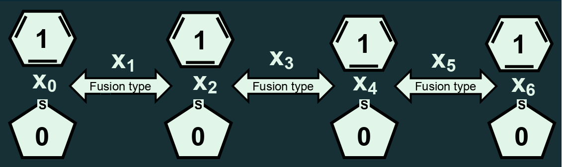
We now describe in detail how the encoding was performed. As described in Figure 1, for the case of , bits , , , and correspond to the structure of the rings, with 0 representing a thiophene ring and 1 representing a benzene ring. () shows how the consecutive rings of and are fused. In the case where and (meaning adding a thiophene ring to a thiophene ring), leads to the structure of thieno[2,3-b]thiophene, and leads to the structure of thieno[3,2-b]thiophene. In the case where and (meaning adding a benzene ring to a thiophene ring), both and lead to the same structure of benzo[b]thiophene, resulting in the presence of duplicates. For the case of adding a ring to a benzene ring ( and ), the definition of becomes more complicated, and the resulting fused structures are detailed in Table 1.
The dataset is complete because it contains the of all compounds represented by the binary strings in the dataset. This allows us to know beforehand which of the encoded compounds has the lowest , and check whether the algorithms are able to predict it. However, for the larger datasets using and , only the of a small portion of the encoded compounds is available, and therefore we cannot know which have the lowest . As described in Section III.4, a sequential learning process is carried to augment these datasets in an informed way.
II.3 molecular datasets
| 0 | 1 | 1 | 0 | 0 | naphtho[2,3-b]thiophene |
| 0 | 1 | 1 | 1 | 0 | naphtho[1,2-b]thiophene |
| 0 | 1 | 1 | 0 | 1 | naphtho[2,1-b]thiophene |
| 0 | 1 | 1 | 1 | 1 | naphtho[1,2-b]thiophene |
| 0 | 1 | 0 | 0 | 0 | benzo[1,2-b:5,4-b’]dithiophene |
| 0 | 1 | 0 | 1 | 0 | benzo[1,2-b:4,5-b’]dithiophene |
| 0 | 1 | 0 | 0 | 1 | benzo[2,1-b:3,4-b’]dithiophene |
| 0 | 1 | 0 | 1 | 1 | benzo[1,2-b:3,4-b’]dithiophene |
| 1 | 1 | 1 | 0 | 0 | phenanthrene*1 |
| 1 | 1 | 1 | 1 | 0 | anthracene |
| 1 | 1 | 1 | 0 | 1 | phenanthrene*1 |
| 1 | 1 | 1 | 1 | 1 | anthracene |
| 1 | 1 | 0 | 0 | 0 | naphtho[2,3-b]thiophene*2 |
| 1 | 1 | 0 | 1 | 0 | naphtho[2,3-b]thiophene*2 |
| 1 | 1 | 0 | 0 | 1 | naphtho[2,1-b]thiophene*3 |
| 1 | 1 | 0 | 1 | 1 | naphtho[1,2-b]thiophene*4 |
*1 In case , and if the pre-determined structure is phenanthrene, this yields chrysene not forming benzo[c]phenanthrene. If naphtho[2,3-b]thiophene, phenanthro[2,3-b]thiophene is formed not forming phenanthro[3,2-b]thiophene. If naphtho[1,2-b]thiophene, phenanthro[1,2-b]thiophene is formed not forming phenanthro[4,3-b]thiophene.
*2 If the pre-determined structure is naphtho[2,3-b]thiophene, naphtho[2,3-b:7,6-b’]dithiophene is formed.
*3 If the pre-determined structure is naphtho[2,3-b]thiophene, naphtho[2,1-b:6,7-b’]dithiophene is formed.
*4 If the pre-determined structure is naphtho[2,3-b]thiophene, naphtho[1,2-b:6,7-b’]dithiophene is formed.
The second dataset uses a N = 16 bits encoding to represent heteroacene structures, in this case with 8 rings, which can again be either benzene or thiophene rings. This dataset contains the reorganization energies (ranging from 0.072 eV to 0.286 eV) of 99 different chemical compounds represented by 926 bitstrings (approximately 9.4 duplicate bitstrings per compound). These 926 bitstrings constitute a very small portion (1.41%) of the total number of possible binary strings with 16 bits, which is = 65536 (the bitstring solution space). We can roughly estimate the number of different heteroacene structures represented by all bitstrings by extrapolating the number of duplicates in the training dataset, resulting in 6972 encoded heteroacene structures (the chemical solution space). In a similar fashion to the N = 7 dataset, 8 bits (one per ring) are used to encode whether a ring is a benzene or a thiophene ring, while the other 8 bits store information about how two adjacent rings are fused. Since there are only 7 fusing sites in a open 8 ring chain, one of the fusion sites is assigned 2 bits so that it can encode 4 fusing options, while the rest of the fusions are represented by only 1 bit.
More precisely, for the case of , bits , , , , , , , and represent the structure of the ring, with 0 being a thiophene ring and 1 being a benzene ring. () shows how the two rings of and are fused, where 1 bit is assigned to describe the scheme of ring fusing. An exception exists for and , which are the 2 bits used to describe the scheme of ring fusing for the two rings of and . For the case where 1 bit is assigned to describe the scheme of ring fusing (), the definition of is the same as that for , except for three specific cases. These exceptions occur when or and :
-
1.
If the pre-determined structure is phenanthrene, a chrysene structure is formed instead of benzo[c]phenanthrene.
-
2.
If the pre-determined structure is naphtho[2,3-b]thiophene, phenanthro[2,3-b]thiophene is formed instead of phenanthro[3,2-b]thiophene.
-
3.
If the pre-determined structure is naphtho[1,2-b]thiophene, phenanthro[1,2-b]thiophene is formed instead of phenanthro[4,3-b]thiophene.
These modifications were made to favor less bent structures and minimize steric hindrance within the molecule.
Next, we describe how and were defined. In the case where and (meaning a thiophene ring is added to a thiophene ring), and lead to the structure of thieno[2,3-b]thiophene, while other cases of and result in the structure of thieno[3,2-b]thiophene. If and (meaning a benzene ring is added to a thiophene ring), any combination of and results in the same structure of benzo[b]thiophene, leading to duplicates. For the case of adding a ring to a benzene ring ( and ), the definitions of and become more complex, and the resulting fused structures are detailed in Table 2.
II.4 N=22 molecular dataset
The final dataset is an expansion of the bits dataset, but using bits to encode the structures. It also contains heteroacene structures with 8 rings that can be either benzene or thiophene. The 6 added extra bits in the encoding are assigned to encode information about the fusing between subsequent molecules, allowing for a greater number of possible 8-ringed heteroacene structures to be represented. In this case, every scheme of ring fusion is assigned 2 bits (in total, 14 bits for encoding ring fusions) so that 4 different fusion schemes can be encoded between adjacent rings. Same as before, the remaining 8 bits encode the type of molecule in each ring. More precisely, , , , , , , , and represent the structure of the ring, with 0 being a thiophene ring and 1 being a benzene ring. and () describe how the two rings of and are fused, with their definition being the same as that for indices and for .
All 99 compounds present in the training dataset are also part of the training dataset, and in addition to these compounds, 20 extra compounds were further added to explore the new subspace spanned by the 6 extra bits. In total, this dataset contains the of 119 different chemical compounds ( ranging from 0.072 eV to 0.286 eV) represented by 24,512 bitstrings (0.58% of the bitstrings solution space), having 206 duplicate bitstrings per compound on average. The bitstring solution space is now approximately 4.2 million (), which represents a total of approximately 20,361 compounds, calculated again by extrapolating the number of duplicate bitstrings in the training dataset.
II.5 Data processing
To train the models in the learning phase of the algorithms, we split the data into a training set and a test set in order to measure the generalization capabilities of the models to unseen data. Recall that our input data are binary strings with an assigned scalar value each (the hole reorganization energy ). Each binary string represents a single chemical compound, but the opposite is not true as each chemical compound may be represented by more than one bitstring (duplicates).
Due to the presence of duplicate bitstrings, one needs to be careful when splitting the data into a training and test set. In fact, we construct two separate test datasets. The first is the non-isolated test dataset, which is constructed with duplicates of bitstrings that are present in the training dataset, meaning that the underlying chemical compound is actually seen during training. Therefore, the performance on this non-isolated data only measures the ability of the model to identify the symmetries in the encoding giving rise to the duplicates, but it does not truly measure generalization to unseen chemical compounds. The second dataset is the isolated test dataset. This dataset contains all duplicates of a number of randomly picked chemical structures that are not part of the training dataset, meaning that no duplicates of those structures are seen during training. Therefore, the performance on this dataset truly measures the ability to generalize to unseen chemical compounds.
For all datasets we do a 8:1:1 split (train/isolated test/non-isolated test) of the data. Furthermore, the data is always normalized to the interval before it is provided as input to the models.
III Algorithmic framework
III.1 Extremal learning
The algorithmic framework used in this work is known as extremal learning [38, 37]. Extremal learning algorithms aim to find the input to a hidden function which extremizes the output of the function , only given partial input-output training data . In our case, both the input and the output of the function are one-dimensional, but extremal learning can be straightforwardly generalized to higher dimensions. Usually, this is achieved via two distinct phases, a learning (or modeling) phase and a selection (or extremization) phase. In the learning phase, a (quantum) machine learning model is trained on the partial training data to build an approximate model of the hidden function . Once is learned, an extremization procedure is performed in the selection phase to find that extremizes the output of the approximate model . If is sufficiently accurate and the extremization process succeeds, will correspond (or be close) to the optimal input of the hidden function, .
Extremal learning algorithms are naturally suited for the task of material discovery where the fitness of a molecule can be faithfully described by one or more figures of merit. In this case, the inputs are the considered family of chemical structures, represented via the chosen encoding, while the output can be any figure of merit that is desirable to extremize; in our case, we wish to minimize the hole reorganization energy . Different extremal learning algorithms can employ different strategies for the learning and selection phase. Depending on the particular algorithm, both phases can be performed via classical or quantum computation.
Here we employ two quantum-enhanced extremal learning algorithms, namely Quantum Extremal Learning (QEL) [38] and Factorization Machine + Quantum Approximate Optimization Algorithm (FM+QAOA) [39]. We use the term ”quantum-enhanced” to remark the fact that these algorithms employ both quantum and classical computation at some point in their workflow. QEL employs a QML algorithm in the learning phase and a classical method in the selection phase, while FM+QAOA follows an opposite approach using a classical ML model in the learning phase and a QML algorithm in the selection phase. Next, we describe both algorithms in detail.
III.2 FM+QAOA
The first extremal learning algorithm is named Factorization Machine+ Quantum Approximate Optimization Algorithm, or FM+QAOA for short. It employs a classical ML model (Factorization Machine) in the learning phase and a quantum algorithm (QAOA) in the selection phase. This method was first proposed in [39], where it was successfully applied to a material design problem.
III.2.1 Learning phase: Factorization Machines
A Factorization Machine (FM) is a supervised classical machine learning algorithm [55] commonly used in recommendation systems [56]. Although in principle a FM model can have any arbitrary order , which allows to capture all -th order correlations between the input features , here we restrict the FM to be second order (). Higher order FMs [57] may provide a more accurate model if the data presents significant higher order correlations, but in the context of the FM+QAOA algorithm it would significantly increase the complexity of the quantum circuit implementing QAOA. Moreover, a second order approximation is enough in many cases, particularly in extremal learning algorithms where high accuracy is not required for the selection phase to succeed.
For binary input vectors a second order FM can be mathematically written as
| (3) |
where are the elements of the factorized matrix of quadratic coefficients. A second order FM captures all single and pairwise interactions between the input features . The pairwise interactions are modeled by factorizing the coefficients in a embedding matrix of size , where is a hyperparameter controlling the degree of factorization. Reducing can help control overfitting as the number of parameters is also reduced, although in this work we fix , thus not performing any factorization.
III.2.2 Selection phase: QAOA
The goal of the selection phase is to find the optimal solution that extremizes the hidden function , using the trained FM model as a proxy. Without loss of generality, we can assume that the solution is the minimum of (if is such that it maximizes then the problem can always be reformulated as ). The task of finding the optimal input minimizing Eq. (3) can be formulated as a Quadratic Unconstrained Binary Optimization (QUBO) problem [58, 59]. Any QUBO problem can be mapped to an Ising Hamiltonian via the transformation , where is the Z-Pauli matrix. The resulting Ising Hamiltonian,
| (4) |
encodes the solution of the QUBO problem in its ground state.
Therefore, the task of finding can be translated to finding the ground state of . A wide range of quantum algorithms for ground state preparation have been proposed, both for fault tolerant [60] and Noisy Intermediate-Scale Quantum (NISQ) [61] devices. Here we use the Quantum Approximate Optimization Algorithm (QAOA) [62, 63, 58], a variational quantum algorithm motivated by a trotterized version of the quantum adiabatic algorithm. The algorithm employs two different operators, a cost operator and a mixing operator defined as
| (5) |
where and are the cost and mixing Hamiltonians, respectively, and are variational parameters. The cost Hamiltonian encodes the solution in its ground state; in our case, it is the Ising Hamiltonian defined by the Factorization Machine, . For the mixing Hamiltonian one may select any Hamiltonian which does not commute with the cost Hamiltonian i.e. . In our case, we choose the standard , where is the X-Pauli matrix applied on qubit .
The final state is prepared by applying successive layers of the cost operators and mixing operators applied to the initial state, which is the ground state of the mixing Hamiltonian, in our case :
| (6) |
The variational parameters are trained with a classical optimizer to minimize the expectation value of the cost Hamiltonian via a quantum-classical feedback loop. If the algorithm converges, sampling the final state in the computational basis should give the state corresponding to the optimal solution with the highest probability. In our simulations we simulate the final sampling process with finite shot noise.
Many variants of QAOA have been proposed to improve its performance and trainability; however, in this work, we employ the originally proposed version explained above. The only algorithmic trick we use relates to the initialization of the variational parameters . In particular, to train a QAOA circuit of depth , we progressively extend the depth of the circuit from a single layer to layers, using the optimal values found with depth as the initial values for the first layers of the circuit of length . This means that in order to train a QAOA circuit of depth , we first need to train circuits with depths , which forces a significant computation overhead. However, this initialization strategy greatly benefits convergence by avoiding local minima [64]. We note that other initialization strategies with lower overhead and similar performance might be available. We leave other possible extensions of QAOA as future continuation of this work.
III.3 Quantum Extremal Learning
The second extremal learning algorithm is the Quantum Extremal Learning algorithm proposed in [38]. In the original paper, both the learning and selection phases employ a quantum approach leveraging Quantum Neural Networks (QNNs) for both continuous and discrete data.
However, when the input data are discrete the selection method proposed in [38] converges to exactly a single solution. To fuel the sequential learning process to expand the and bits datasets (explained in Section III.4), we require the algorithm to generate 50 candidate solutions in each iteration. For this reason, we only use the original selection method for the smallest N=7 dataset, where no sequential learning process is carried since the dataset is already complete. For the larger datasets, we instead use a brute-force method for selecting the best candidates, explained in Section III.3.2. Note that neither the brute-force method used here nor the selection method used in [38] are efficient; further work is required to design a more efficient selection procedure in QEL.
III.3.1 Learning phase: Quantum Neural Networks
The learning phase in QEL is carried by a Quantum Neural Network (QNN), which we denote as the learning QNN. We define a QNN as a variational quantum circuit acting on a -qubit register. The quantum circuit used here consists of two parts: a feature map and a variational ansatz . The feature map is used to encode the classical input data into the circuit:
| (7) |
where is the quantum state resulting from the action of the feature map on the initial state . Since in our case the input data are binary strings of length , we use a basis encoding where a bitstring is mapped onto the corresponding computational basis state (e.g. the bitstring is mapped into the the computational state ). This feature map can be easily implemented via a layer of gates acting on the qubits that correspond to a bit value 1, leveraging the fact that .
After encoding the classical data into , a variational ansatz is applied. In our case, is a Hardware-Efficient Ansatz (HEA) [65] consisting of layers of single qubit rotations acting on qubit and layer , interleaved with entangling blocks of chained CNOTs. Information is extracted from the circuit by performing a measurement at the end, in our case the average local magnetization . The variational parameters are optimized such that the expectation value of the measurement operator matches the hidden function for each bitstring
| (8) |
The predicted function can be differentiated with respect to through the parameter shift rule [66] (although in our numerical experiments we use automatic differentiation as we emulate the quantum algorithms in classical hardware), so standard gradient-based optimization routines can be used to find the optimal values of . We use additional trainable parameters for the scaling and shifting of the output, , and we always normalize the data to the be in the range before feeding it to the model.
An important benefit of using a QNN compared to a second order FM in the learning phase is that a QNN can model correlations of arbitrary order between the input features , given an appropriate ansatz. Although a Factorization Machine can also be generalized to arbitrary order (mapping the data to a general -order Hamiltonian instead of an Ising Hamiltonian), this may require very deep circuits when implementing the cost operator in the QAOA circuit, rendering the latter approach very computationally demanding for large .
III.3.2 Selection phase
Different selection methods are required in QEL depending on whether the input data is continuous or discrete. The continuous case is straightforward, as we can leverage the fact that the right-hand side of Eq. (8) is differentiable with respect to the feature map parameters and run a gradient-descent optimization routine to find the optimal input . However, when the data is discrete, the differentiability vanishes, so an alternative approach needs to be employed to find the extremal input.
Throughout this work, we use two different selection methods tailored to discrete data, depending on the dataset we are dealing with. For the smallest dataset , we follow the approach presented in [38], where the discrete feature map in the quantum circuit is substituted by a selection QNN, whose action is denoted by the unitary , with continuous variational parameters . This unitary generates the state
| (9) |
After convergence, this state should have major support on the quantum state corresponding to the optimal input , i.e. . In our case, we choose to be a Hardware-Efficient Ansatz with the same architecture as in the learning phase. Since is differentiable with respect to , a gradient-descent optimization routine can be employed to find the optimal parameters . Once it has successfully converged, the optimal parameters can be extracted by sampling the state .
However, in order for to represent the optimal solution, the optimization routine needs to be adjusted to account for the fact that the data is discrete. To showcase this adjustment, let us write the state as a linear combination of computational basis states:
| (10) |
where and are the computational basis states of qubits. The loss we aim to minimize can then be written as
| (11) | ||||
The loss can be written as the sum of two terms: a diagonal term containing the diagonal matrix elements and a cross term containing the non-diagonal elements . Only minimizing the diagonal term contributes to the state becoming the optimal state. Therefore, we only use the diagonal term, i.e. we minimize . Computing only the diagonal term involves calculating the exponential sum in each optimization step, and therefore it is not an efficient procedure.
A consequence of the above adjusted optimization process is that the state usually converges to only the single best computational state. In general, it is ideal that the final state has no support on other states that are close to optimal, but for the purposes of the sequential learning process described in Section III.4, we would like the selection algorithm to output the best states (we fix in our case) so that we can expand the dataset with a meaningful number of candidates at each iteration. In order to circumvent this issue, for the large datasets with and , we employ a simpler selection routine based on a brute-force approach sorting the bitstrings by their corresponding predicted energy, based on the trained quantum model. Although this naive approach is also not efficient, and thus it cannot be scaled to a large number of qubits, it allows us to select an arbitrary number of candidates, so that the sequential learning process can be carried. Furthermore, using the brute-force approach, we are guaranteed to find the correct extremal inputs of the model resulting from the learning phase.
III.4 Sequential learning process
Sequential learning (SL) [33, 34, 35, 36] refers to the process of iteratively updating a model to guide (physical or computational) experiments. In a SL process, the model actively solicits new data to improve its performance, creating a feedback loop between the experimental results and the model’s training process. SL has been shown to be useful in materials science as it can reduce the number of compounds that need to be evaluated through DFT calculations [67, 35] or chemical synthesis [68]. Since these evaluations usually constitute the most expensive part of the material discovery pipeline, SL can greatly speed up material discovery algorithms.
In our case, SL offers an ideal avenue to expand the limited amount of initial training data available for the and datasets. Recall that the amount of data initially available to us is just 927 bitstrings (corresponding to 99 chemical structures) for the dataset and 24512 bitstrings (119 chemical structures) for the dataset, representing 1.41% and 0.58% of the bitstring solution space, respectively. To circumvent this issue, we follow a SL process where we use the predictions of our algorithms to iteratively expand the training data. At each iteration, a set of 50 candidate bitstrings is generated, corresponding to the chemical structures predicted to be most optimal, i.e., to have the lowest predicted reorganization energy . Next, DFT methods are used to compute the true reorganization energy of the chemical compounds represented by those candidate bitstrings. At this stage, all duplicate bitstrings representing the predicted chemical structures are identified and incorporated into the dataset. By augmenting the training dataset with the compounds predicted to have the lowest in the previous iteration, we aim to bias the model towards predicting low- compounds. Note that despite the fact that 50 bitstrings are generated at each iteration, some of the predicted bitstrings might be duplicates which represent the same chemical structure. Therefore, usually less than 50 new unique chemical compounds are added in each iteration. On the other hand, due to the added duplicates, more than 50 new bitstrings are added at each iteration.
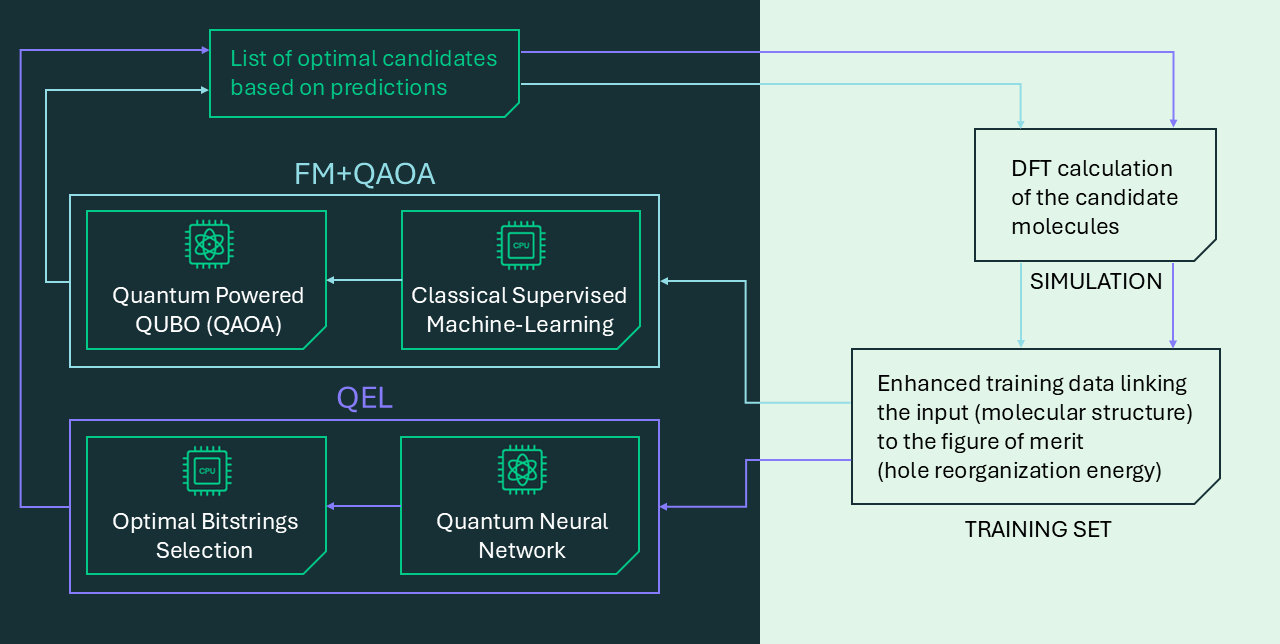
As a result of the SL process, both the size and quality of the dataset increase with each iteration, as the added compounds are predicted by the algorithm to have low . Consequently, the algorithms should improve at predicting low- structures as the SL process advances. This SL process is done independently for both the FM+QAOA and the QEL algorithm, meaning that no data exchange occurs between them and each algorithm has no knowledge of the predictions of the other. This is made explicit in Figure 2 by the two independent arrows representing the independent flow of information for the FM+QAOA (blue arrows) and QEL (purple arrows).
At every iteration, 30 instances of each algorithm were run, each instance with different portions of the data assigned to the train and test sets as well as different initial parameters. Out of these 30 instances, we filtered the instances achieving a mean absolute error (MAE) on the isolated test dataset (see Section II.5) greater than a certain threshold. Given that our only focus is to build models that generalize well to the low- regime, we only focus on the MAE of compounds with a eV. The training process of each instance was also stopped at the point achieving the lowest MAE in these low- compounds, in order to improve the accuracy of the models in this regime. We use the MAE and not the score because the latter may not be accurate when calculated on samples drawn from a narrow range (the variance in the denominator might diverge), which is the case when we focus solely on the low- regime.
IV Numerical results
In this Section, we discuss the performance of the FM+QAOA and QEL algorithms applied to the three molecular datasets described in Section II.2. The datasets were benchmarked with both the FM+QAOA and the QEL algorithms, while the dataset was only tested with the FM+QAOA algorithm.
The numerical results presented here were computed in a classical computer cluster employing CPU and GPU resources, and all quantum algorithms were programmed with Qadence [69]. Derivatives were computed through automatic differentiation, enabled through Qadence’s Pytorch backend [70, 71]. No noise was considered other than finite shot noise when sampling the final state in QAOA. Regarding training, all models were trained with the ADAM optimizer [72] using a decaying learning rate strategy.
IV.1 N=7 dataset
We start with the smallest dataset built with the N=7 bits encoding. The dataset contains 54 different chemical structures represented by 128 bitstrings of length 7. This is the only dataset where we have access to the figure of merit (the DFT-calculated hole reorganization energy ) for all bitstrings in the solution space. This allows us to perform a thorough analysis of the algorithms’ performance by leveraging the fact that we know the optimal solution beforehand.
IV.1.1 Hyperparameter tuning
To ensure a fair comparison between the two algorithms, we conducted a hyperparameter search to identify optimal hyperparameter settings for each training dataset size. For the FM+QAOA algorithm, the most important hyperparameter is the number of layers of the QAOA algorithm. Theoretically, increasing the QAOA depth should always give greater accuracy, with asymptotical guarantees at the infinite depth limit. However, in practice the variational parameters might not converge to optimal values because the training process might become very hard for large depths. For the dataset, our numerical experiments revealed that the performance of the QAOA algorithm was not significantly influenced by the depth of QAOA. In fact, for all training dataset sizes, performance plateaued when the QAOA depth exceeded 4 layers. Consequently, the depth was fixed at 4 layers for the remainder of the experiments with . Finally, we used shots to sample the final state of QAOA.
The main hyperparameter in the QEL algorithm is the depth of the Quantum Neural Networks (QNNs) used in the learning and selection phase. In this case, we performed a grid search to study the performance of the QNNs with depth ranging from 2 to 8 layers by looking at the cross-validation score averaged over 25 instances for each depth. Table 3 shows the optimal number of layers for different training dataset sizes. We observe that as the amount of training data increases, the optimal depth of the learning QNN also increases. This is likely because training a QNN that is too deep on insufficient data can lead to overfitting. Increasing the amount of training data allows for deeper QNNs, which are more expressive, while avoiding overfitting. On the other hand, the optimal depth of the selection QNN remains approximately constant for different training dataset sizes. This is likely because the selection QNN does not aim to model any data, but rather to represent the quantum state corresponding to the optimal solution. Since we are only minimizing a function instead of learning the function, there is no need to increase the depth when the amount of training data increases. For the rest of this Section we fix the depths of the QNNs to the values shown in Table 3.
| 0.2 | 0.4 | 0.6 | 0.8 | 1.0 | |
|---|---|---|---|---|---|
| Optimal depth learning QNN | 4 | 5 | 6 | 7 | 7 |
| Optimal depth selection QNN | 3 | 4 | 3 | 3 | 4 |

IV.1.2 Results
Figure 3 shows the performance of both algorithms with the optimal hyperparameter configuration. We measure the performance for different ratios , where is the number of training samples and is the total number of samples (in this case ).
For each ratio, 25 instances of the algorithms were trained with different portions of the data assigned to the train/test sets and different initial parameters. The top plot of Figure 3 showcases the performance of the models in the learning phase using as a figure of merit the average score of the 25 seeds. The score is defined as
| (12) |
where are the input bitstrings in the dataset, is the predicted reorganization energy by the model and is the DFT-calculated reorganization energy. The mean score achieved by QEL is better than the FM when using only 20% of the data for training, which indicates better generalization. However, the QEL algorithm only outperforms the FM algorithm for very small or very large training datasets, and achieves a comparable performance for medium sizes = 0.4 and 0.6. An important observation is that the FM is not able to achieve a perfect score even when using all data for training (), because the FM cannot model the higher order correlations present in the dataset. On the other hand, the QNN in the QEL algorithm does achieve when trained with the whole dataset because it is able to model the higher order correlations successfully.
The bottom plot in Figure 3 shows the results in the selection phase, using as a figure of merit the normalized frequency with which the algorithms found the optimal solution. This is, out of the 25 instances, we count how many times the algorithm predicted the compound with the lowest reorganization energy as the most optimal, and then normalize the result. In this case, the FM+QAOA algorithm outperforms the QEL algorithm for all of the training dataset sizes except for the lowest amount of training data, . This also indicates that the QEL algorithm can generalize better when very few training data is used, but on the other hand it performs worse with larger amounts of training data.
An important take-away of Figure 3 is that the models in the learning phase are not required to be very accurate for an extremal learning algorithm to succeed in finding close-to-optimal solutions. In fact, even though QEL was able to model the molecular dataset better than the FM model, the extremization results of QEL are worse than with FM+QAOA for most ratios except when . The reason behind is that as long as the model correctly captures the position of the global extremum point, that should be enough for the selection method to find the solution if the selection process succeeds.
IV.2 N=16 dataset

We now move to benchmarking the algorithms with the larger datasets, starting with the dataset. Recall that this dataset contains the DFT-calculated hole reorganization energies of 99 different chemical compounds represented by 927 bitstrings (approximately 9.4 duplicate bitstrings per compound). Since 16 bits are now used to encode the molecules, the complete bitstring solution space is now composed of all possible bitstrings of length 16, significantly larger compared to the previous dataset. Importantly, now we only have access to the of a small fraction () of the solution space, meaning that we cannot check if a predicted candidate is the optimal solution because we do not know which is the lowest reorganization energy compound in the solution space.
Alternatively, we focus on whether the algorithms are able to predict structures with , where eV is the lowest reorganization energy in both the initial and datasets. We denote any such compound as an extrapolative compound. Finding an extrapolative compound means that the algorithm can successfully generalize to molecules in the low- regime.
IV.2.1 Hyperparameter tuning
Following the same procedure as with the dataset, we performed a hyperparameter search to determine the optimal settings for the algorithms. Regarding QEL, recall that for the and datasets we do not use a selection QNN, but rather a brute-force approach which does not have any hyperparameters. Therefore, only the depth of the learning QNN had to be tuned, for which a grid search was carried with depths ranging from 4 to 14. The optimal depth was determined to be 8 layers by looking at the score on the isolated test averaged over 5 instances. In the FM+QAOA, the depth of the QAOA circuit was fixed to 16 layers and the final state was sampled with shots.
IV.2.2 Results
Figure 5 depicts a box plot visualization of the DFT-calculated hole reorganization energy of the selected candidates by each algorithm during the different iterations of the sequential learning process. The FM+QAOA algorithm, when applied to the dataset, demonstrates a consistent trend of improvement, with the of the predicted candidates increasingly clustering within the low- regime (defined to be the region eV). On the other hand, QEL shows more variability, with some iterations failing to converge (e.g. iterations 1 and 4). However, both algorithms are able to focus the predictions in the low- regime by the later stages of the sequential learning process, especially after iteration 6, achieving similar final distributions.
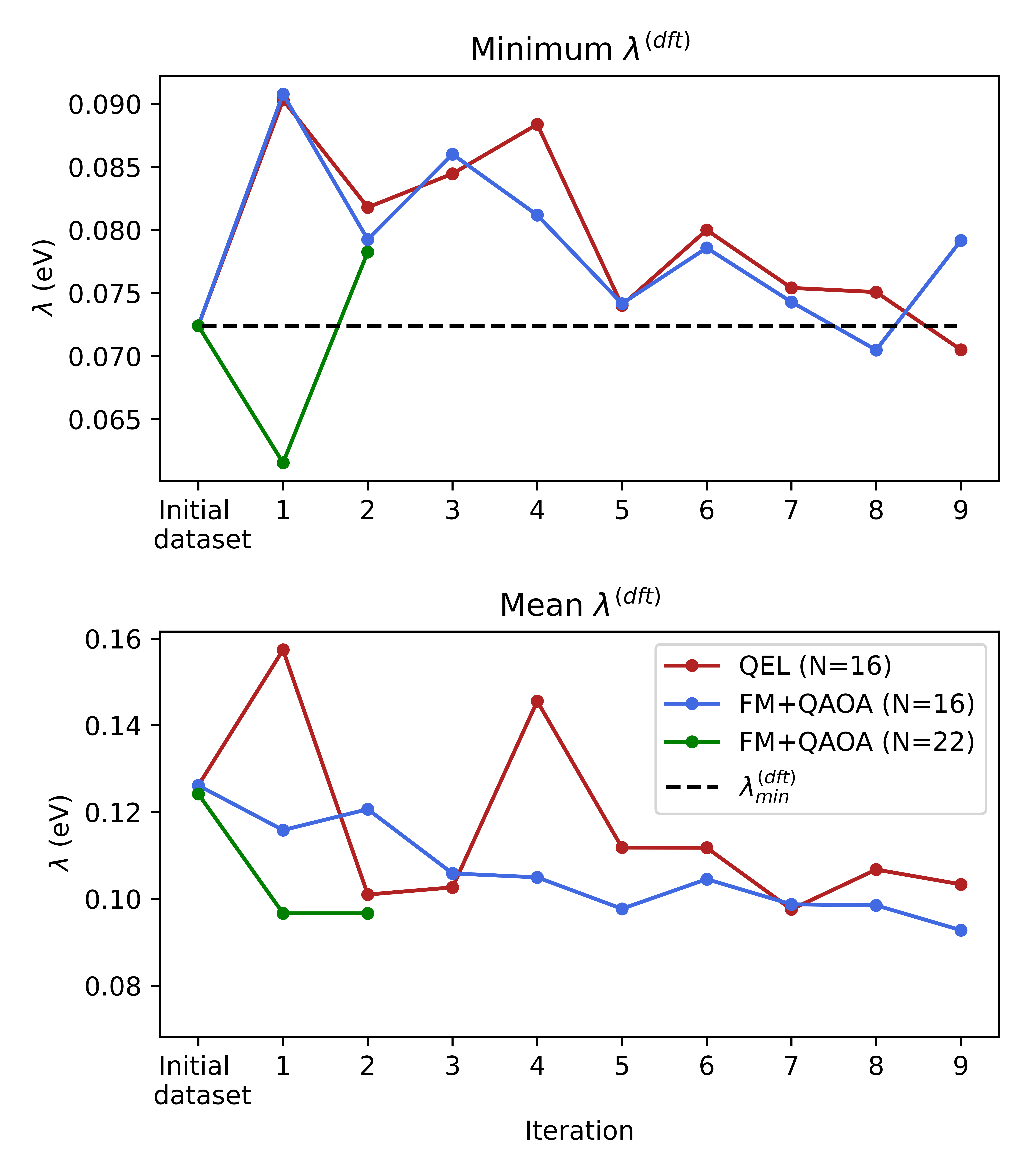
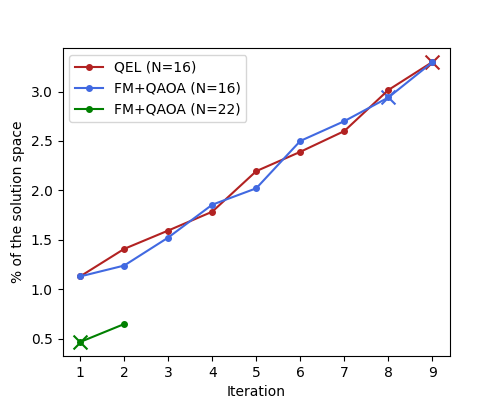
It is illustrative to focus on the lowest reorganization energy compound predicted at each iteration, shown more clearly in the top plot of Figure 4. Recall that we aim to predict chemical structures with a lower than the minimum in the initial dataset ( eV), marked by the dashed black line in the plot. Both FM+QAOA and QEL closely follow each other predicting similar minimum , with the FM+QAOA performing slightly better in most iterations. In the first iterations, the lowest energy compounds have energies close to 0.085 eV. Once enough training data have been added through the sequential learning process (from iteration 4 onward), both algorithms are able to predict compounds with a minimum close to 0.075 eV. Finally, the FM+QAOA algorithm predicts an extrapolative compound in iteration 8 using of the solution space for training. The predicted candidate has =0.071 eV, and its chemical structure is shown in Figure 9a. The QEL algorithm achieved extrapolation one iteration later, at iteration 9, and it predicted the same compound as the FM+QAOA with eV. The QEL algorithm required a slightly larger training dataset than the FM+QAOA, using 3.33% of the solution space for training. Given that the sequential learning processes for both algorithms are completely independent to each other, it is remarkable that both QEL and FM+QAOA identified the same compound at almost the same iteration. Figure 7 shows the size of the training dataset in each iteration, relative to the total number of possible bitstrings in the solution space.
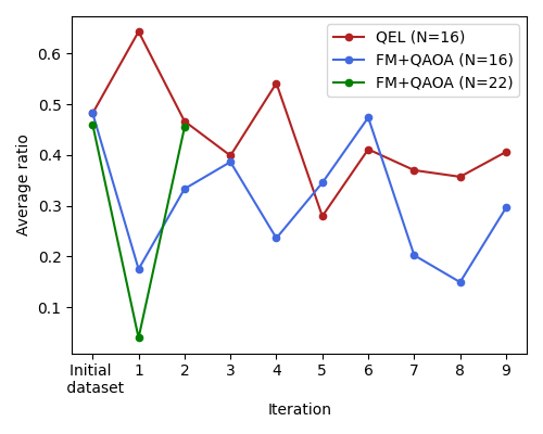
The bottom plot in Figure 4 shows the mean of the predicted candidates in each iteration. Again, the FM+QAOA consistently decreases the mean of the predictions, while in QEL it sharply increases in the iterations where it failed to converge. Nevertheless, both algorithms reach mean energies around 0.1 eV by the last few iterations, showing again a similar performance by the end of the sequential learning process.
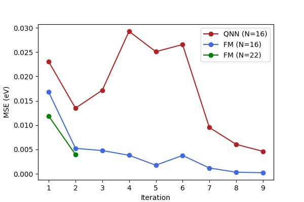
Up until now, we have discussed the overall performance of the algorithms based on the quality of the predicted candidates. However, it is also interesting to solely focus on the performance of the models in the learning phase, as it constitutes a crucial step towards a working extremal learning algorithm. Recall that the goal of the learning phase is to construct a model of the data that the selection algorithm can subsequently use to identify optimal candidates. Figure 6 shows the Mean Squared Error (MSE) of the reorganization energy of the predicted candidates across iterations. In particular, it shows the MSE of the predicted by the models in the learning phase with respect to the values calculated using DFT for the candidate compounds. Recall that the FM+QAOA uses a Factorization Machine (FM) as a model in the learning phase, while QEL uses a Quantum Neural Network (QNN). The FM consistently outperforms the QNN in terms of MSE across all iterations for the dataset. This improvement is especially pronounced in the mid-iterations (4 to 7), where QEL exhibits a noticeable spike in the MSE values. Furthermore, the FM seems to consistently improve with each iteration, while the QEL algorithm again shows a more inconsistent progress, which is in line with our earlier observations.
IV.3 N=22 dataset
We now move to the largest dataset that was investigated, constructed with a bits encoding. We recall that it contains 119 different heteroacene compounds represented by 24512 bitstrings (approximately 206 duplicate bitstrings per chemical compound). In this case, only the FM+QAOA algorithm was trained with this dataset, as the computational resources to emulate QEL with 22 qubits were too large without drawing upon approximation methods such as tensor networks [73], that were not considered in this work. Given the large computational requirements, the depth of the QAOA circuit was limited to 14 layers, and where used to sample the final QAOA state.
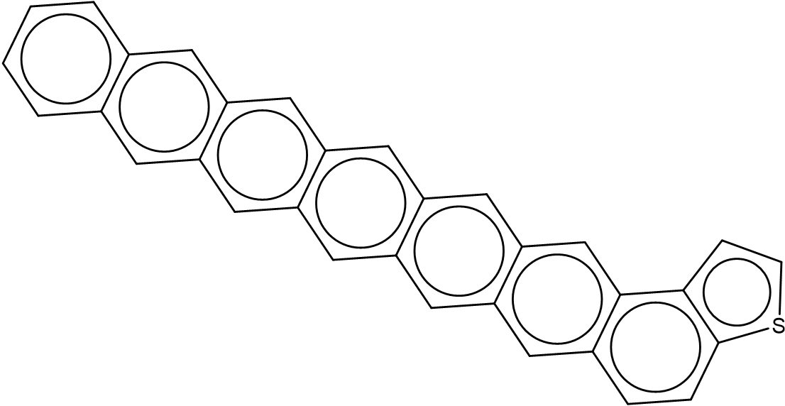
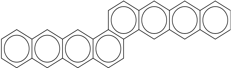
The FM+QAOA performed very well with the 22 bits dataset, predicting octacene as an extrapolative compound with =0.062 eV already at the first iteration (see Figures 4 and 5). This was achieved using 19873 bitstrings for training, which represents 0.47% of the bitstring solution space. Even though the absolute number of bitstrings used for training to achieve extrapolation is larger than in the , it represents a significant reduction in terms of relative size to the total number of bitstrings, as the FM+QAOA required 2.94% and QEL 3.33% to predict an extrapolative design with . Therefore, we can observe that as the solution space grows, the absolute amount of data needed for extrapolation increases, but the fraction of the solution space needed for effective learning decreases.
The structure of the predicted extrapolative molecule was also very interesting (linear structure with no 5-membered rings), and we note that such structures have also been identified as a low- structure in a previous study [17]. One more iteration was done after achieving extrapolation at iteration 1, which did not provide any compounds with lower despite improving the mean of the predicted compounds (bottom plot of Figure 4).
IV.4 Chemical insights


Having discussed the algorithmic performance, we now dedicate the rest of the Section to the chemical insights arising from the compounds predicted by the quantum-enhanced algorithms.
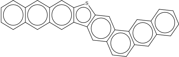
Figure 9 shows different hetereoacene structures that were predicted by or used for training in the algorithms, together with their DFT-calculated hole reorganization energies. The compound in Figure 9a is the extrapolative design predicted by the FM+QAOA and QEL algorithms with the dataset at iterations 8 and 9, respectively. In Figure 9b the extrapolative compound (octacene) predicted by the FM+QAOA with the dataset is presented. There are two properties worth noting in this heteroacene structure. Firstly, we observe that the structure is completely linear, as all rings in the chain are connected along a straight line. Secondly, none of the rings contain heteratoms, so that all rings are 6-membered. The latter aligns well with previous research, where a low ratio of 5-membered rings in heteroacene structures has been linked to low hole reorganization energies with the most preferable range of the ratio being 0.2-0.4 in terms of minimizing the reorganization energy [1]. In fact, Figure 8 shows how as the sequential learning process advances, the ratio of 5-membered rings in the predicted candidate compounds also tends to decrease. This is in line with our previous reasoning because as iterations pass, the of the predicted candidates also decreases, due to the training dataset improving in both size and quality.
It is remarkable that the FM+QAOA algorithm was able to extrapolate to the low energy compound in Figure 9b with the dataset already in the first iteration, using only 0.47% of the bitstring solution space for training. Upon further examination of the training dataset, we found two compounds with a very similar structure to 9b which also have low reorganization energy (both with eV). These two compounds, shown in Figures 9c and 9d, are equal to octacene in all but the last ring, where a thiophene ring is present instead of a benzene ring, with the sulfur heteroatom placed differently in each of them. Also, the compounds are ”semi-linear” in the sense that only the last ring containing the heteroatom is not oriented following the line defined by the rest of the rings.
In order to check the effect of the two semi-linear compounds on the algorithm predicting the extrapolative compound, we run the first iteration of the FM+QAOA algorithm again but removing the two semi-linear compounds from the dataset. As it turned out, the FM+QAOA algorithm was still able to predict the extrapolative compound 9b. In fact, another compound with low reorganization energy eV was predicted which also had a semi-linear structure with all rings being 6-membered (benzenes), shown in Figure 9e. In conclusion, the results of this alternative first iteration were similar to the original run, with 21 out of the 50 best selected bitstrings overlapping, indicating that the presence of the two semi-linear compounds was not the main cause behind the FM+QAOA algorithm finding the extrapolative compound. We should keep in mind that we are analyzing the results of a single iteration of the sequential learning process, and therefore a lot of variability can be expected, especially given the vast size of the solution space with bits. This means that no strong conclusions can be derived from the fact that the algorithm performed slightly better without the two semi-linear compounds.
V Conclusions
In this work, we have explored the use of two quantum-enhanced algorithms for a materials discovery task. Specifically, we aimed to predict heteroacene structures with low hole reorganization energy , which is a reliable estimator of the carrier mobility in organic semiconductors. The algorithms employed here follow the extremal learning framework, which consists of a learning phase where a ML model is trained to fit the data and a selection phase where the optimal (or extremal) candidates are selected. The algorithms are quantum-enhanced because in each of them a different phase is done via a quantum algorithm: in QEL, the learning phase is quantum while the selection phase is classical, whereas in FM+QAOA, the learning phase is classical and the selection phase is quantum.
Our numerical experiments showed that both algorithms were able to predict heteroacene structures with lower hole reorganization energy than the lowest energy compound present in the initial dataset ( eV), which we denote as an extrapolative compounds, proving good generalization capabilities to the low- regime. When trained with the dataset, the FM+QAOA and QEL algorithms predicted an extrapolative compound with eV after 8 and 9 iterations of the sequential learning process, respectively. Both achieved a similar performance in terms of the lowest predicted reorganization energies, although the QEL algorithm offered less consistent predictions and less accurate models in the learning phase. Furthermore, the FM+QAOA was also applied to a larger dataset with , predicting a compound (octacene) with eV already in the first iteration while using a smaller portion of the solution space for training compared to the case. Crucially, the previous extrapolative structures were suggested whilst working on samples of a classically curated dataset deriving from a massive theoretical screening of M molecules and a record eV. This observation makes the final results presented in this paper with few iterations and a much smaller dataset far from trivial. These results also suggest that improved performance can be achieved by increasing the number of bits in the encoding, paving the way to the application of such algorithms to datasets encoding a larger chemical space.
The predicted low- compounds offered interesting chemical insights, as they presented two key common features: a linear or semi-linear structure and a majority of 6-membered rings. This is in line with previous research where it has been shown that such structures tend to show low values of [1, 17]. For example, octacene is found to be the lowest compound in our study, whereas in a previous study, nonacene is listed as one of the lowest- compounds that were de novo designed [17].
In conclusion, this work aimed to explore quantum-enhanced extremal learning algorithms in realistic, state-of-art scenarios of materials discovery, focusing on variational algorithms amenable to implementation in near-term quantum processors. The numerical results presented in this work were computed via noiseless emulation on large classical computing resources. In order to unlock the benefits from the quantum stage of our algorithms, further work studying the scalability and quantum-hardware implementation must be carried. Future work could focus on improving the scaling of the proposed algorithms with the size of the datasets. For example, in QEL, the brute-force selection could be substituted with a QNN adapted to extremize over discrete inputs, or the training process of the QAOA algorithm could be subject to improvements to benefit convergence in larger circuits. Our results, although necessarily limited, offer an exciting prospect regarding the use of Quantum Machine Learning for material discovery.
Acknowledgements.
IFG and SV thank Antonio A. Gentile, Arthur M. Faria, Anton Quelle and Jaap Kautz for useful discussions and valuable feedback, Sylvain Maret for his help administering the HPC resources, Daniel Guijo for his project management skills and Vincent E. Elfving for his initial help setting up the project.References
- [1] N. N. Matsuzawa, H. Arai, M. Sasago, E. Fujii, A. Goldberg, T. J. Mustard, H. S. Kwak, D. J. Giesen, F. Ranalli, and M. D. Halls, “Massive theoretical screen of hole conducting organic materials in the heteroacene family by using a cloud-computing environment,” The Journal of Physical Chemistry A, vol. 124, no. 10, pp. 1981–1992, Mar 2020. [Online]. Available: https://doi.org/10.1021/acs.jpca.9b10998
- [2] Y. Liu, T. Zhao, W. Ju, and S. Shi, “Materials discovery and design using machine learning,” Journal of Materiomics, vol. 3, no. 3, pp. 159–177, 2017, high-throughput Experimental and Modeling Research toward Advanced Batteries. [Online]. Available: https://www.sciencedirect.com/science/article/pii/S2352847817300515
- [3] K. Rajan, “Materials informatics,” Materials Today, vol. 8, no. 10, pp. 38–45, 2005.
- [4] J. E. Anthony, “Functionalized acenes and heteroacenes for organic electronics,” Chemical Reviews, vol. 106, no. 12, pp. 5028–5048, Dec 2006. [Online]. Available: https://doi.org/10.1021/cr050966z
- [5] I. F. Perepichka, D. F. Perepichka, H. Meng, and F. Wudl, “Light-emitting polythiophenes,” Adv. Mater., vol. 17, no. 19, pp. 2281–2305, 2005.
- [6] M. J. Kang, I. Doi, H. Mori, E. Miyazaki, K. Takimiya, M. Ikeda, and H. Kuwabara, “Alkylated dinaphtho[2,3-b:2’,3’-f]thieno[3,2-b]thiophenes (cn-dntts): Organic semiconductors for high-performance thin-film transistors,” Adv. Mater., vol. 23, no. 10, pp. 1222–1225, 2011.
- [7] A. B. Sieval and J. Hummelen, “Fullerene-based acceptor materials,” in Organic Photovoltaics, C. Brabec, U. Scherf, and V. Dyakonov, Eds. Wiley, 2024, pp. 209–238.
- [8] H. Li, B. C.-K. Tee, J. J. Cha, Y. Cui, J. W. Chung, S. Y. Lee, and Z. Bao, “High-mobility field-effect transistors from large-area solution-grown aligned c60 single crystals,” J. Am. Chem. Soc., vol. 134, no. 5, pp. 2760–2765, 2012.
- [9] J. Takeya, M. Yamagishi, Y. Tominari, R. Hirahara, Y. Nakazawa, T. Nishikawa, T. Kawase, T. Shimoda, and S. Ogawa, “Very high-mobility organic single-crystal transistors with in-crystal conduction channels,” Appl. Phys. Lett., vol. 90, no. 10, p. 102120, 2007.
- [10] M. B. Prince, “Drift mobilities in semiconductors. ii. silicon,” Phys. Rev., vol. 93, no. 6, pp. 1204–1206, 1954.
- [11] R. A. Marcus, “On the theory of oxidation-reduction reactions involving electron transfer. i,” J. Chem. Phys., vol. 24, no. 5, pp. 966–978, 1956.
- [12] ——, “On the theory of oxidation-reduction reactions involving electron transfer. ii. applications to data on the rates of isotopic exchange reactions,” J. Chem. Phys., vol. 26, no. 4, pp. 867–871, 1957.
- [13] ——, “On the theory of oxidation-reduction reactions involving electron transfer. iii. applications to data on the rates of organic redox reactions,” J. Chem. Phys., vol. 26, no. 4, pp. 872–877, 1957.
- [14] ——, “On the theory of electron-transfer reactions. vi. unified treatment for homogeneous and electrode reactions,” J. Chem. Phys., vol. 43, no. 2, pp. 679–701, 1965.
- [15] C. Schober, K. Reuter, and H. Oberhofer, “Virtual screening for high carrier mobility in organic semiconductors,” J. Phys. Chem. Lett., vol. 7, no. 19, pp. 3973–3977, 2016.
- [16] F. H. Allen, “The cambridge structural database: A quarter of a million crystal structures and rising,” Acta Crystallogr., Sect. B: Struct. Sci., vol. 58, no. 3-1, pp. 380–388, 2002.
- [17] G. Marques, K. Leswing, T. Robertson, D. Giesen, M. D. Halls, A. Goldberg, K. Marshall, J. Staker, T. Morisato, H. Maeshima, H. Arai, M. Sasago, E. Fujii, and N. N. Matsuzawa, “De novo design of molecules with low hole reorganization energy based on a quarter-million molecule dft screen,” The Journal of Physical Chemistry A, vol. 125, no. 33, pp. 7331–7343, Aug 2021. [Online]. Available: https://doi.org/10.1021/acs.jpca.1c04587
- [18] C. Kunkel, C. Schober, J. T. Margraf, K. Reuter, and H. Oberhofer, “Finding the right bricks for molecular legos: A data mining approach to organic semiconductor design,” Chem. Mater., vol. 31, no. 3, pp. 969–978, 2019.
- [19] S. Nagasawa, E. Al-Naamani, and A. Saeki, “Computer-aided screening of conjugated polymers for organic solar cell: Classification by random forest,” J. Phys. Chem. Lett., vol. 9, no. 10, pp. 2639–2646, 2018.
- [20] E. Antono, N. N. Matsuzawa, J. Ling, J. E. Saal, H. Arai, M. Sasago, and E. Fujii, “Machine-learning guided quantum chemical and molecular dynamics calculations to design novel hole-conducting organic materials,” J. Phys. Chem. A, vol. 124, no. 40, pp. 8330–8340, 2020.
- [21] T. Ando, N. Shimizu, N. Yamamoto, N. N. Matsuzawa, H. Maeshima, and H. Kaneko, “Design of molecules with low hole and electron reorganization energy using dft calculations and bayesian optimization,” J. Phys. Chem. A, vol. 126, no. 36, pp. 6336–6347, 2022.
- [22] J. Staker, K. Marshall, K. Leswing, T. Robertson, M. D. Halls, A. Goldberg, T. Morisato, H. Maeshima, T. Ando, H. Arai, M. Sasago, E. Fujii, and N. N. Matsuzawa, “De novo design of molecules with low hole reorganization energy based on a quarter-million molecule dft screen: Part 2,” J. Phys. Chem. A, vol. 126, no. 34, pp. 5837–5852, 2022.
- [23] L. Clinton, T. Cubitt, B. Flynn, F. M. Gambetta, J. Klassen, A. Montanaro, S. Piddock, R. A. Santos, and E. Sheridan, “Towards near-term quantum simulation of materials,” Nature Communications, vol. 15, no. 1, Jan. 2024. [Online]. Available: http://dx.doi.org/10.1038/s41467-023-43479-6
- [24] R. Babbush, N. Wiebe, J. McClean, J. McClain, H. Neven, and G. K.-L. Chan, “Low-depth quantum simulation of materials,” Physical Review X, vol. 8, no. 1, Mar. 2018. [Online]. Available: http://dx.doi.org/10.1103/PhysRevX.8.011044
- [25] Y. Alexeev, M. Amsler, M. A. Barroca, S. Bassini, T. Battelle, D. Camps, D. Casanova, Y. J. Choi, F. T. Chong, C. Chung, C. Codella, A. D. Córcoles, J. Cruise, A. Di Meglio, I. Duran, T. Eckl, S. Economou, S. Eidenbenz, B. Elmegreen, C. Fare, I. Faro, C. S. Fernández, R. N. B. Ferreira, K. Fuji, B. Fuller, L. Gagliardi, G. Galli, J. R. Glick, I. Gobbi, P. Gokhale, S. de la Puente Gonzalez, J. Greiner, B. Gropp, M. Grossi, E. Gull, B. Healy, M. R. Hermes, B. Huang, T. S. Humble, N. Ito, A. F. Izmaylov, A. Javadi-Abhari, D. Jennewein, S. Jha, L. Jiang, B. Jones, W. A. de Jong, P. Jurcevic, W. Kirby, S. Kister, M. Kitagawa, J. Klassen, K. Klymko, K. Koh, M. Kondo, D. M. Kürkçüoglu, K. Kurowski, T. Laino, R. Landfield, M. Leininger, V. Leyton-Ortega, A. Li, M. Lin, J. Liu, N. Lorente, A. Luckow, S. Martiel, F. Martin-Fernandez, M. Martonosi, C. Marvinney, A. C. Medina, D. Merten, A. Mezzacapo, K. Michielsen, A. Mitra, T. Mittal, K. Moon, J. Moore, S. Mostame, M. Motta, Y.-H. Na, Y. Nam, P. Narang, Y. ya Ohnishi, D. Ottaviani, M. Otten, S. Pakin, V. R. Pascuzzi, E. Pednault, T. Piontek, J. Pitera, P. Rall, G. S. Ravi, N. Robertson, M. A. Rossi, P. Rydlichowski, H. Ryu, G. Samsonidze, M. Sato, N. Saurabh, V. Sharma, K. Sharma, S. Shin, G. Slessman, M. Steiner, I. Sitdikov, I.-S. Suh, E. D. Switzer, W. Tang, J. Thompson, S. Todo, M. C. Tran, D. Trenev, C. Trott, H.-H. Tseng, N. M. Tubman, E. Tureci, D. G. Valiñas, S. Vallecorsa, C. Wever, K. Wojciechowski, X. Wu, S. Yoo, N. Yoshioka, V. W. zhe Yu, S. Yunoki, S. Zhuk, and D. Zubarev, “Quantum-centric supercomputing for materials science: A perspective on challenges and future directions,” Future Generation Computer Systems, vol. 160, pp. 666–710, 2024. [Online]. Available: https://www.sciencedirect.com/science/article/pii/S0167739X24002012
- [26] M. Schuld, R. Sweke, and J. J. Meyer, “Effect of data encoding on the expressive power of variational quantum-machine-learning models,” Physical Review A, vol. 103, no. 3, Mar. 2021. [Online]. Available: http://dx.doi.org/10.1103/PhysRevA.103.032430
- [27] M. C. Caro, H.-Y. Huang, M. Cerezo, K. Sharma, A. Sornborger, L. Cincio, and P. J. Coles, “Generalization in quantum machine learning from few training data,” Nature Communications, vol. 13, no. 1, Aug. 2022. [Online]. Available: http://dx.doi.org/10.1038/s41467-022-32550-3
- [28] K. Takimiya, S. Shinamura, I. Osaka, and E. Miyazaki, “Thienoacene-based organic semiconductors,” Adv. Mater., vol. 23, no. 38, pp. 4347–4370, 2011.
- [29] A. Shinamura, E. Miyazaki, and K. Takimiya, “Synthesis, properties, crystal structures, and semiconductor characteristics of naphtho-[1,2-b:5,6-b’]dithiophene and -diselenophene derivatives,” J. Org. Chem., vol. 75, no. 4, pp. 1228–1234, 2010.
- [30] T. Okamoto, C. Mitsui, M. Yamagishi, K. Nakahara, J. Soeda, Y. Hirose, K. Miwa, H. Sato, A. Yamano, T. Matsushita, T. Uemura, and J. Takeya, “V-shaped organic semiconductors with solution processability, high mobility, and high thermal durability,” Adv. Mater., vol. 25, no. 44, pp. 6392–6397, 2013.
- [31] A. Okamoto, Y. Murata, C. Mitsui, H. Ishii, M. Yamagishi, M. Yano, H. Sato, A. Yamano, J. Takeya, and T. Okamoto, “Zigzag-elongated fused p-electronic core: A molecular design strategy to maximize charge-carrier mobility,” Adv. Sci., vol. 5, no. 1, p. 1700317, 2018.
- [32] S. Haas, Y. Takahashi, K. Takimiya, and T. Hasegawa, “High-performance dinaphtho-thieno-thiophene single crystal field-effect transistors,” Applied Physics Letters, vol. 95, no. 2, p. 022111, 2009. [Online]. Available: https://doi.org/10.1063/1.3183509
- [33] B. Rohr, H. S. Stein, D. Guevarra, Y. Wang, J. A. Haber, M. Aykol, S. K. Suram, and J. M. Gregoire, “Benchmarking the acceleration of materials discovery by sequential learning,” Chemical science, vol. 11, no. 10, pp. 2696–2706, 2020.
- [34] A. Palizhati, S. B. Torrisi, M. Aykol, S. K. Suram, J. S. Hummelshøj, and J. H. Montoya, “Agents for sequential learning using multiple-fidelity data,” Scientific Reports, vol. 12, no. 1, p. 4694, Mar 2022. [Online]. Available: https://doi.org/10.1038/s41598-022-08413-8
- [35] C. Völker, R. Firdous, D. Stephan, and S. Kruschwitz, “Sequential learning to accelerate discovery of alkali-activated binders,” Journal of materials science, vol. 56, pp. 15 859–15 881, 2021.
- [36] P. V. Balachandran, D. Xue, J. Theiler, J. Hogden, and T. Lookman, “Adaptive strategies for materials design using uncertainties,” Scientific Reports, vol. 6, no. 1, p. 19660, Jan 2016. [Online]. Available: https://doi.org/10.1038/srep19660
- [37] Z. Patel and M. Rummel, “Extremal learning: extremizing the output of a neural network in regression problems,” 2021. [Online]. Available: https://arxiv.org/abs/2102.03626
- [38] S. Varsamopoulos, E. Philip, V. E. Elfving, H. W. T. van Vlijmen, S. Menon, A. Vos, N. Dyubankova, B. Torfs, and A. Rowe, “Quantum extremal learning,” Quantum Machine Intelligence, vol. 6, no. 2, p. 42, Jul 2024. [Online]. Available: https://doi.org/10.1007/s42484-024-00176-x
- [39] K. Kitai, J. Guo, S. Ju, S. Tanaka, K. Tsuda, J. Shiomi, and R. Tamura, “Designing metamaterials with quantum annealing and factorization machines,” Phys. Rev. Res., vol. 2, p. 013319, Mar 2020. [Online]. Available: https://link.aps.org/doi/10.1103/PhysRevResearch.2.013319
- [40] W. Kohn and L. J. Sham, “Self-consistent equations including exchange and correlation effects,” Phys. Rev., vol. 140, pp. A1133–A1138, Nov 1965. [Online]. Available: https://link.aps.org/doi/10.1103/PhysRev.140.A1133
- [41] P. Hohenberg and W. Kohn, “Inhomogeneous electron gas,” Phys. Rev., vol. 136, pp. B864–B871, Nov 1964. [Online]. Available: https://link.aps.org/doi/10.1103/PhysRev.136.B864
- [42] W.-Q. Deng and W. A. G. III, “Predictions of hole mobilities in oligoacene organic semiconductors from quantum mechanical calculations,” Journal of Physical Chemistry B, vol. 108, no. 25, pp. 8614–8621, 2004. [Online]. Available: https://doi.org/10.1021/jp0495848
- [43] L. Schrödinger, “Schrödinger release 2021-3: Materials science suite,” 2021, accessed Feb. 2025. [Online]. Available: https://www.schrodinger.com/platform
- [44] A. D. Becke, “Density-functional thermochemistry: Iii. the role of exact exchange,” Journal of Chemical Physics, vol. 98, no. 7, pp. 5648–5652, 1993. [Online]. Available: https://doi.org/10.1063/1.464913
- [45] C. Lee, W. Yang, and R. G. Parr, “Development of the colle-salvetti correlation-energy formula into a functional of the electron density,” Physical Review B, vol. 37, no. 2, pp. 785–789, 1988. [Online]. Available: https://doi.org/10.1103/PhysRevB.37.785
- [46] R. Ditchfield, W. A. Hehre, and J. A. Pople, “Self-consistent molecular orbital methods. ix. extended gaussian-type basis for molecular-orbital studies of organic molecules,” J. Chem. Phys., vol. 54, no. 2, pp. 724–728, 1971. [Online]. Available: https://doi.org/10.1063/1.1674902
- [47] P. J. Hay and W. R. Wadt, “Ab initio effective core potentials for molecular calculations. potentials for the transition metal atoms sc to hg,” J. Chem. Phys., vol. 82, no. 1, pp. 270–283, 1985. [Online]. Available: https://doi.org/10.1063/1.448799
- [48] ——, “Ab initio effective core potentials for molecular calculations. potentials for main group elements na to bi,” J. Chem. Phys., vol. 82, no. 1, pp. 284–298, 1985. [Online]. Available: https://doi.org/10.1063/1.448800
- [49] ——, “Ab initio effective core potentials for molecular calculations. potentials for k to au including the outermost core orbitals,” J. Chem. Phys., vol. 82, no. 1, pp. 299–310, 1985. [Online]. Available: https://doi.org/10.1063/1.448975
- [50] A. D. Bochevarov, E. Harder, T. F. Hughes, J. Greenwood, D. Braden, D. M. Philipp, D. Rinaldo, M. D. Halls, J. Zhang, and R. A. Friesner, “Jaguar: A high-performance quantum chemistry software program with strengths in life and materials sciences,” Int. J. Quantum Chem., vol. 113, no. 18, pp. 2110–2142, 2013. [Online]. Available: https://doi.org/10.1002/qua.24481
- [51] L. Schrödinger, “Jaguar release 2021-3: Materials science suite,” 2021, https://www.schrodinger.com/platform/products/jaguar (accessed Feb. 2025). [Online]. Available: https://www.schrodinger.com/platform/products/jaguar
- [52] D. Weininger, “Smiles, a chemical language and information system. 1. introduction to methodology and encoding rules,” Journal of Chemical Information and Computer Sciences, vol. 28, no. 1, pp. 31–36, Feb 1988. [Online]. Available: https://doi.org/10.1021/ci00057a005
- [53] A. Mauri, V. Consonni, and R. Todeschini, Molecular Descriptors. Cham: Springer International Publishing, 2017, pp. 2065–2093. [Online]. Available: https://doi.org/10.1007/978-3-319-27282-5_51
- [54] C. Wang, Y. Yang, J. Song, and X. Nan, “Research progresses and applications of knowledge graph embedding technique in chemistry,” Journal of Chemical Information and Modeling, vol. 64, no. 19, pp. 7189–7213, Oct 2024. [Online]. Available: https://doi.org/10.1021/acs.jcim.4c00791
- [55] Y. Koren, R. Bell, and C. Volinsky, “Matrix factorization techniques for recommender systems,” Computer, vol. 42, no. 8, pp. 30–37, 2009.
- [56] C. A. Gomez-Uribe and N. Hunt, “The netflix recommender system: Algorithms, business value, and innovation,” ACM Trans. Manage. Inf. Syst., vol. 6, no. 4, Dec. 2016. [Online]. Available: https://doi.org/10.1145/2843948
- [57] M. Blondel, A. Fujino, N. Ueda, and M. Ishihata, “Higher-order factorization machines,” 2016. [Online]. Available: https://arxiv.org/abs/1607.07195
- [58] K. Blekos, D. Brand, A. Ceschini, C.-H. Chou, R.-H. Li, K. Pandya, and A. Summer, “A review on quantum approximate optimization algorithm and its variants,” Physics Reports, vol. 1068, p. 1–66, Jun. 2024. [Online]. Available: http://dx.doi.org/10.1016/j.physrep.2024.03.002
- [59] A. Lucas, “Ising formulations of many np problems,” Frontiers in Physics, vol. 2, 2014. [Online]. Available: http://dx.doi.org/10.3389/fphy.2014.00005
- [60] L. Lin and Y. Tong, “Near-optimal ground state preparation,” Quantum, vol. 4, p. 372, Dec. 2020. [Online]. Available: http://dx.doi.org/10.22331/q-2020-12-14-372
- [61] J. Tilly, H. Chen, S. Cao, D. Picozzi, K. Setia, Y. Li, E. Grant, L. Wossnig, I. Rungger, G. H. Booth, and J. Tennyson, “The variational quantum eigensolver: A review of methods and best practices,” Physics Reports, vol. 986, p. 1–128, Nov. 2022. [Online]. Available: http://dx.doi.org/10.1016/j.physrep.2022.08.003
- [62] E. Farhi, J. Goldstone, and S. Gutmann, “A quantum approximate optimization algorithm,” 2014. [Online]. Available: https://arxiv.org/abs/1411.4028
- [63] L. Zhou, S.-T. Wang, S. Choi, H. Pichler, and M. D. Lukin, “Quantum approximate optimization algorithm: Performance, mechanism, and implementation on near-term devices,” Physical Review X, vol. 10, no. 2, Jun. 2020. [Online]. Available: http://dx.doi.org/10.1103/PhysRevX.10.021067
- [64] X. Lee, Y. Saito, D. Cai, and N. Asai, “Parameters fixing strategy for quantum approximate optimization algorithm,” in 2021 IEEE International Conference on Quantum Computing and Engineering (QCE). IEEE, Oct. 2021, p. 10–16. [Online]. Available: http://dx.doi.org/10.1109/QCE52317.2021.00016
- [65] A. Kandala, A. Mezzacapo, K. Temme, M. Takita, M. Brink, J. M. Chow, and J. M. Gambetta, “Hardware-efficient variational quantum eigensolver for small molecules and quantum magnets,” Nature, vol. 549, no. 7671, p. 242–246, Sep. 2017. [Online]. Available: http://dx.doi.org/10.1038/nature23879
- [66] K. Mitarai, M. Negoro, M. Kitagawa, and K. Fujii, “Quantum circuit learning,” Physical Review A, vol. 98, no. 3, Sep. 2018. [Online]. Available: http://dx.doi.org/10.1103/PhysRevA.98.032309
- [67] J. H. Montoya, K. T. Winther, R. A. Flores, T. Bligaard, J. S. Hummelshøj, and M. Aykol, “Autonomous intelligent agents for accelerated materials discovery,” Chem. Sci., vol. 11, pp. 8517–8532, 2020. [Online]. Available: http://dx.doi.org/10.1039/D0SC01101K
- [68] M. M. Noack, P. H. Zwart, D. M. Ushizima, M. Fukuto, K. G. Yager, K. C. Elbert, C. B. Murray, A. Stein, G. S. Doerk, E. H. R. Tsai, R. Li, G. Freychet, M. Zhernenkov, H.-Y. N. Holman, S. Lee, L. Chen, E. Rotenberg, T. Weber, Y. L. Goc, M. Boehm, P. Steffens, P. Mutti, and J. A. Sethian, “Gaussian processes for autonomous data acquisition at large-scale synchrotron and neutron facilities,” Nature Reviews Physics, vol. 3, no. 10, pp. 685–697, Oct 2021. [Online]. Available: https://doi.org/10.1038/s42254-021-00345-y
- [69] D. Seitz, N. Heim, J. P. Moutinho, R. Guichard, V. Abramavicius, A. Wennersteen, G.-J. Both, A. Quelle, C. de Groot, G. V. Velikova, V. E. Elfving, and M. Dagrada, “Qadence: a differentiable interface for digital and analog programs,” IEEE Software, pp. 1–14, 2025.
- [70] Pasqal, “Pyqtorch.” [Online]. Available: https://github.com/pasqal-io/pyqtorch
- [71] A. Paszke, S. Gross, S. Chintala, G. Chanan, E. Yang, Z. DeVito, Z. Lin, A. Desmaison, L. Antiga, and A. Lerer, “Automatic differentiation in pytorch,” in NIPS-W, 2017.
- [72] D. P. Kingma and J. Ba, “Adam: A method for stochastic optimization,” 2017. [Online]. Available: https://arxiv.org/abs/1412.6980
- [73] K. Bidzhiev, A. Wennersteen, M. Beji, M. Dagrada, M. D’Arcangelo, S. Grijalva, A.-C. L. Henaff, A. Quelle, and A. S. Naik, “Cloud on-demand emulation of quantum dynamics with tensor networks,” 2023. [Online]. Available: https://arxiv.org/abs/2302.05253