CM-Diff: A Single Generative Network for Bidirectional Cross-Modality Translation Diffusion Model Between Infrared and Visible Images

Abstract

The image translation method represents a crucial approach for mitigating information deficiencies in the infrared and visible modalities, while also facilitating the enhancement of modality-specific datasets. However, existing methods for infrared and visible image translation either achieve unidirectional modality translation or rely on cycle consistency for bidirectional modality translation, which may result in suboptimal performance. In this work, we present the cross-modality translation diffusion model (CM-Diff) for simultaneously modeling data distributions in both the infrared and visible modalities. We address this challenge by combining translation direction labels for guidance during training with cross-modality feature control. Specifically, we view the establishment of the mapping relationship between the two modalities as the process of learning data distributions and understanding modality differences, achieved through a novel Bidirectional Diffusion Training (BDT) strategy. Additionally, we propose a Statistical Constraint Inference (SCI) strategy to ensure the generated image closely adheres to the data distribution of the target modality. Experimental results demonstrate the superiority of our CM-Diff over state-of-the-art methods, highlighting its potential for generating dual-modality datasets.

1 Introduction

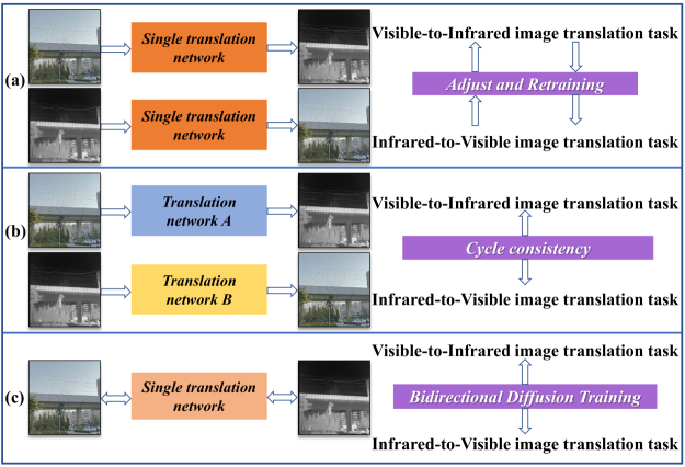
Figure 1: Comparison of infrared-visible image translation methods: (a) Unidirectional methods require network modifications and retraining to enable translation in the opposite direction; (b) existing bidirectional methods employ two independent generative networks and utilize cycle consistency for simultaneous training; (c) CM-Diff introduces Bidirectional Diffusion Training (BDT) strategy, eliminating the need for separate networks and reducing the computational overhead and retraining time associated with unidirectional methods.

Infrared and visible imaging are two common modalities in visual perception within the computer vision community. Infrared images are captured on the basis of the thermal radiation emitted by objects, which makes them invariant to illumination conditions and robust against environmental disturbances such as low light and smoke [24]. However, they lack color, texture, and detailed information, which limits their ability to analyze fine-grained objects. On the other hand, visible images are formed by the reflection of light from objects, providing rich color, texture, and detailed information, enabling precise object representation and fine-grained analysis. This disparity in the characteristics of infrared and visible imaging creates a complementary relationship between the two modalities, making their integration or alternation crucial for robust real-world applications. Given the complementary strengths and limitations of visible and infrared imaging, dual-modality methods often outperform single-modality methods, particularly in tasks like object detection [9], [8], [21] and semantic segmentation [26], [18], [3]. However, these methods usually rely on a large, well-aligned dual-modality dataset, while in practice, acquiring such registered dual-modality datasets is challenging and costly. Thus, a natural idea is to leverage image translation techniques to generate dual-modality datasets.

Recent infrared-visible image translation methods have achieved promising results using Generative Adversarial Networks (GANs) [28, 40, 13, 48, 27, 10, 29, 47, 5, 17, 42, 30, 2, 34, 12] and Denoising Diffusion Probabilistic Models (DDPMs) [6, 38, 32, 23, 33], which can be broadly classified into two categories: bidirectional image translation methods and unidirectional image translation methods. Bidirectional methods [48, 27, 10, 29, 38] typically employ two independent generative networks to establish mappings between the infrared and visible modalities, often relying on a cycle consistency method, as shown in Fig. 1 (b). Although the cycle consistency based methods have proven to be effective in ensuring modality correspondence, it not only increases the complexity of the network architecture but also frequently leads to perceptual blurriness and loss of fine details in the generated outputs [48, 31]. Unidirectional methods [47, 5, 17, 42, 30, 2, 34, 12, 32] leverage a single generative network to model the mapping in one direction, either infrared-to-visible image translation or vice versa. Consequently, they require separate training processes for each translation direction to achieve bidirectional modality translation, as shown in Fig. 1 (a).

In this paper, we propose a unified framework called CM-Diff. The core idea is to enable joint learning of infrared and visible image data using a Bidirectional Diffusion Training (BDT) strategy, as shown in Fig. 1 (c). This method incorporates implicit prompts through input channel positions, combined with explicit directional label embedding. This method is further refined by a multi-level Cross-modality Feature Control (CFC), which enhances semantic control over the translation process. Consequently, it eliminates reliance on the cycle-consistency method while enabling more precise mapping between the two data modalities. Furthermore, we observe that after implementing bidirectional conversion, the issue of color distortion becomes critically severe when directly applying the original ancestral sampling method [19, 43] for infrared-visible image translation. To address this, we propose a Statistical Constraint Inference (SCI) strategy, which leverages statistical mean constraints tailored to different datasets and scenarios. By incorporating these statistical properties, we mitigate abnormalities caused by the inherent randomness in the reverse Markov chain of DDPM, ensuring that the generated images maintain high fidelity and align closely with real-world distributions. The main contributions of this paper can be summarized as follows:

1. A unified framework called CM-Diff is proposed for bidirectional translation between infrared and visible images. The method employs a Bidirectional Diffusion Training (BDT) strategy, which incorporates direction labels and source domain image features. These components guide the model to distinctly learn the distributions of two domains. By establishing an inherent mapping between them, the method improves the quality and accuracy of the translated images.

2. By incorporating distributional information with the Statistical Constraint Inference (SCI) strategy, the proposed method effectively eliminates anomalies in the reverse Markov chain paths. This enables the model to better align the generated image distribution with the real data distribution.

3. Experimental results demonstrate the superiority and effectiveness of our approach, highlighting its potential in addressing modality absence and misalignment issues.

2 Related Work

Cross-modality translation methods between infrared and visible images can generally be categorized into GAN-based and DDPM-based approaches.

2.1 GAN-based Cross-modality Image Translation

GAN-based models, renowned for their ability to generate high-quality images and capture complex data distributions, have been widely applied in the infrared-visible modality image translation.

The infrared-to-visible image translation task presents notable challenges due to the absence of color and semantic information in infrared images compared to visible images. Typically, GAN-based methods address this task by converting single-channel infrared images into three-channel visible images to support downstream tasks, such as object detection [29], face recognition [47], and other related tasks. To enhance the learning of local sparse structures, TVA-GAN [42] integrates attention mechanisms and employs deep feature extraction using an inception network, achieving state-of-the-art generative performance. In order to extend infrared-to-visible image translation to videos, I2V-GAN [22] proposed an improved cyclic constraint along with content and style perceptual losses, as well as similarity losses, to enhance temporal smoothness and semantic detail preservation. To enhance the utilization of scene information and achieve improved semantic consistency in the translation results, EADS [37] introduced an edge-assisted generation approach to enhance structural information in infrared images, while ROMA [44] proposed a cross-domain similarity matching technique to improve structural correspondence, producing smoother video outputs.

Although visible images contain abundant details and color information, translating them into infrared images that accurately represent thermal radiation remains a significant challenge. This challenge arises due to the inherent differences in imaging mechanisms between visible and infrared modalities. Consequently, the visible-to-infrared image translation task transforms three-channel visible images into single-channel infrared images, addressing the gap in their imaging characteristics while preserving shared semantic information to support downstream tasks. For instance, rgb2nir [1] facilitates the conversion of visible images in remote sensing scenarios to near-infrared images, providing valuable data for agricultural operations and experimental studies. Furthermore, Patch Loss and Fourier Transform Loss, as introduced in VTF-GAN [34], are employed to capture spatial and frequency domain information. This approach generates thermally consistent and detail-preserving infrared facial images, which can aid in medical diagnostics (e.g., inflammation detection) and emotional state analysis. In aerial imagery, IC-GAN [2] introduces a mapper module that transforms the generator’s output into a multi-level color space with learnable weights. This transformation aims to reduce the distance between paired visible and infrared images, thereby enhancing forest fire monitoring. Additionally, methods such as TMGAN-NCC and TMGAN-MP [30] transform visible images in remote sensing into infrared images, supporting object detection and template matching tasks.

Although GAN-based methods excel in generating high-quality images, they often suffer from training instability and mode collapse. In contrast, our approach leverages DDPM to ensure more stable and reliable generation outcomes.

2.2 DDPM-based Cross-modality Imge Translation

Denoising Diffusion Probabilistic Models avoid the training instability and mode collapse often encountered in GANs by using a Markov chain with forward and reverse diffusion processes to transform complex image distributions into simple Gaussian distributions. In the field of infrared-to-visible image translation, T2V-DDPM [32] proposed a method using DDPM for translating infrared to visible facial images. This method addresses the challenge posed by low-light conditions in surveillance, a context in which infrared imaging proves effective for capturing information, whereas face recognition algorithms often fail due to the lack of sufficient visible features. In addition, UNIT-DDPM [38] leveraged the DDPM to avoid stability issues associated with adversarial training and introduced a dual-domain Markov chain to simultaneously approximate the source and target modalities, and it explored the image translation between infrared and visible modalities.

Generally speaking, these unidirectional translation methods can achieve high-quality translation results in one direction, but they require retraining to perform the translation task in the opposite direction. Bidirectional translation methods, relying on cycle consistency, typically require two separate translation networks, which may lead to potential performance degradation. Both approaches struggle to achieve high-quality cross-modality bidirectional image translation. In contrast, our proposed unified framework effectively handles both translation tasks within a single training session, circumventing the network structural complexity associated with the cycle consistency method and mitigating potential degradation in translation result quality.

3 Method

Figure 2: Overview of CM-Diff. (a) Bidirectional Diffusion Training (BDT) strategy: Learning domain-specific data distributions and establishing robust bidirectional mappings. (b) Statistical Constraint Inference (SCI) strategy: Ensuring consistency between the statistical distributions of translated images and those in the training data. (c) CM-Diff Architecture: Comprising Cross-Modality Feature Control (CFC), Translation Direction Guidance (TDG), and the Feature Representation and Reconstruction Network. CM-Diff processing a noisy input image by integrating edge feature maps and conditional modality images. CFC aligning noise translation with the reverse direction of semantic content in the conditional modality. TDG guiding the predicted noise toward the expected modality’s reverse direction. Finally, the network predicting the output noise.

Given a set of paired infrared images $\mathcal{X}^{\textsc{ir}}=\{\mathbf{x}^{\textsc{ir}}_{1},\dots,\mathbf{x}^{\textsc{ir}}_{N}\mid\mathbf{x}\in\mathbb{R}^{H\times W\times C_{\textsc{ir}}}\}$ and visible images $\mathcal{X}^{\textsc{vis}}=\{\mathbf{x}^{\textsc{vis}}_{1},\dots,\mathbf{x}^{\textsc{vis}}_{N}\mid\mathbf{x}\in\mathbb{R}^{H\times W\times C_{\textsc{vis}}}\}$, our goal is to train a model $\mathcal{Z}_{N}$ capable of translating infrared images $\mathcal{X}^{\textsc{ir}}$ into their corresponding visible counterparts $\hat{\mathcal{X}}^{\textsc{vis}}$, while also being able to perform the reverse translation from visible images $\mathcal{X}^{\textsc{vis}}$ to infrared images $\hat{\mathcal{X}}^{\textsc{ir}}$. To accomplish this task, we propose a bidirectional end-to-end framework, CM-Diff.

3.1 Bidirectional Diffusion Training (BDT)

Paired infrared (IR) and visible (VIS) images contain similar semantic information, but their data distributions differ significantly due to the distinct imaging characteristics of each modality. To simultaneously learn these two data distributions and establish a bidirectional mapping relationship, we propose a Bidirectional Diffusion Training (BDT) strategy. Our strategy uses a U-Net architecture network, as shown in Fig. 2 (a), to simultaneously learn and distinguish the visible modality data $\mathbf{x}_{0}^{\textsc{vis}}\in\mathcal{X}^{\textsc{vis}}$ and infrared modality data $\mathbf{x}_{0}^{\textsc{ir}}\in\mathcal{X}^{\textsc{ir}}$, and institutes an effective bidirectional mapping to ensure that the content of the source modality image corresponds effectively to the translated target modality image, thereby achieving a stable training process.

1) Translation Direction Guidance (TDG): We first employ an implicit input channel position encoding to determine whether the data distribution being learned is from the infrared modality or the visible modality. Specifically, for the infrared-to-visible translation part, the input consists of three components: the noisy data $q\left(\mathbf{x}^{\textsc{vis}}_{t}\mid\mathbf{x}^{\textsc{vis}}_{0}\right)\in\mathbb{R}^{H\times W\times C_{\textsc{vis}}}$ in the visible modality at time step $t$, the infrared modality image data $\mathbf{x}^{\textsc{ir}}_{0}\in\mathbb{R}^{H\times W\times C_{\textsc{ir}}}$, and the edge feature maps $E^{\textsc{ir}}=\text{DexiNed}\left(\mathbf{x}^{\textsc{ir}}\right)\in\mathbb{R}^{H\times W\times E}$ extracted from the infrared image using the edge detection network DexiNed [39]. For the consistency of subsequent operations, we duplicate the single-channel infrared image across three channels to match the visible format, ensuring $C_{\textsc{vis}}=C_{\textsc{ir}}=3$. Using edge feature maps extracted from infrared and visible images as part of the input prompt can ensure the consistency of the target image [37]. To construct the network input, we concatenate these data along the channel dimension, resulting in the following input representation:

$$\mathcal{Z}_{\text{{ir}-to-{vis}}}^{t}=q\left(\mathbf{x}_{t}^{\textsc{vis}}\mid\mathbf{x}^{\textsc{vis}}_{0}\right)\oplus\mathbf{x}^{\textsc{ir}}_{0}\oplus E^{\textsc{ir}},$$ (1)

where $\mathcal{Z}_{\text{{ir}-to-{vis}}}^{t}\in\mathbb{R}^{H\times W\times\left(C_{\textsc{vis}}+C_{\textsc{ir}}+E\right)}$, $\oplus$ denotes the concatenation operation, with the target modality data, source modality data, and edge features corresponding to channel index ranges $\{1,2,\dots,C_{\textsc{vis}}\}$, $\{C_{\textsc{vis}}+1,C_{\textsc{vis}}+2,\dots,C_{\textsc{ir}}+C_{\textsc{vis}}\}$, and $\{C_{\textsc{ir}}+C_{\textsc{vis}}+1,C_{\textsc{ir}}+C_{\textsc{vis}}+2,\dots,C_{\textsc{ir}}+C_{\textsc{vis}}+E\}$, respectively. This implicit channel encoding effectively distinguishes the data from different modalities without requiring explicit direction labels indicating the data source. Additionally, we introduce label embedding layers $\tau_{\phi}$ to process the translation direction labels, which represent: $\mathcal{C}^{\textsc{ir}}$ corresponding to the image translation direction from visible to infrared, learning the data distribution of the infrared modality.

2) Cross-modality Feature Control (CFC): To achieve effective target-modality image content control based on the source-modality image, in addition to the direct input of edge feature maps, we also train two independent U-Net encoders, one serving as the infrared modality encoder $\mathcal{Z}_{E}^{\textsc{ir}}$ and the other as the visible modality encoder $\mathcal{Z}_{E}^{\textsc{vis}}$, to extract modality features $F_{d}$ from the infrared or visible images. These modality features are then fed into the cross-attention layer of $\mathcal{Z}_{N}$ to enhance the control of the target modality image content. The query $Q_{n}^{i}$, key $K_{n}^{i}$, and value $V_{n}^{i}$ are computed as follows:

$$Q_{n}^{i}=Conv_{q}^{i}\left(F_{g_{i}}^{n}\right),\quad K_{n}^{i},V_{n}^{i}=Conv_{kv}^{i}\left(F_{d_{i}}^{n}\right),$$ (2)

where $F_{g_{i}}^{n}$ is the input vector obtained by flattening the noise feature map of the $i$-th cross-attention part in the $n$-th layer of network $\mathcal{Z}_{N}$, and $F_{d_{i}}^{n}$ is the feature map extracted from the $i$-th part in the $n$-th layer of the modality encoder. Through the cross-modality attention mechanism, we compute the attention weights $A^{i}$ and obtain the updated feature output $F_{g_{i+1}}^{n}$:

$$F_{g_{i+1}}^{n}=F_{g_{i}}^{n}+{softmax}\left(\frac{Q_{n}^{i}\cdot\left(K_{n}^{i}\right)^{T}}{\sqrt{d}}\right)\cdot V_{n}^{i}.$$ (3)

3) Modality Joint Learning Loss Function: Once the model effectively learns to capture the characteristics of both data distributions, we compute the noise prediction loss in each translation direction. Specifically, when the infrared image provides guidance, the mean squared error (MSE) between the predicted noise in the noisy visible image and the true noise is calculated, yielding $\mathcal{L}_{\text{{ir}-to-{vis}}}$. Conversely,when the visible image provides guidance, the corresponding MSE is computed for the infrared image, resulting in $\mathcal{L}_{\text{{vis}-to-{ir}}}$ . The loss functions are defined as:

$$\mathcal{L}_{\text{{ir}-to-{vis}}}\left(\phi\right)=\mathbb{E}_{t_{1},\mathbf{x}_{0}^{\textsc{ir}},\epsilon_{1}}\left[\left\|\epsilon_{1}-\epsilon_{\phi}\left(\mathcal{Z}_{\text{{ir}-to-{vis}}}^{t_{1}},J^{\textsc{vis}},t_{1}\right)\right\|_{2}^{2}\right]$$ (4)

$$\mathcal{L}_{\text{{vis}-to-{ir}}}\left(\phi\right)=\mathbb{E}_{t_{2},\mathbf{x}_{0}^{\textsc{vis}},\epsilon_{2}}\left[\left\|\epsilon_{2}-\epsilon_{\phi}\left(\mathcal{Z}_{\text{{vis}-to-{ir}}}^{t_{2}},J^{\textsc{ir}},t_{2}\right)\right\|_{2}^{2}\right],$$

where $t_{1},t_{2}\overset{\text{i.i.d.}}{\sim}\mathrm{DiscreteUniform}(\{1,\dots,T\})$, $\epsilon_{1},\epsilon_{2}\overset{\text{i.i.d.}}{\sim}\mathcal{N}\left(\mathbf{0},\mathbf{I}\right)$, $J=\tau_{\phi}\left(\mathcal{C}\right)$ . The modality joint learning loss $\mathcal{L}_{{joint}}$ is as follows:

$$\mathcal{L}_{{joint}}\left(\phi\right)=\lambda_{\text{{ir}-to-{vis}}}\cdot\mathcal{L}_{\text{{ir}-to-{vis}}}+\lambda_{\text{{vis}-to-{ir}}}\cdot\mathcal{L}_{\text{{vis}-to-{ir}}}.$$ (5)

The overall training process based on the BDT is presented in Algorithm 1.

Algorithm 1 CM-Diff Training

0: visible (VIS) image $\mathbf{x}^{\textsc{vis}}$, infrared (IR) image $\mathbf{x}^{\textsc{ir}}$, infrared-to-visible direction label $\mathcal{C}^{\textsc{ir}}$, visible-to-infrared direction label $\mathcal{C}^{\textsc{vis}}$.

1: repeat

2:  $\mathbf{x}^{\textsc{vis}}\in\mathcal{X}^{\textsc{vis}},\mathbf{x}^{\textsc{ir}}\in\mathcal{X}^{\textsc{ir}}$

3:  $t_{1},t_{2}\overset{\text{i.i.d.}}{\sim}\mathrm{DiscreteUniform}(\{1,\dots,T\})$

4:  $\epsilon_{1},\epsilon_{2}\overset{\text{i.i.d.}}{\sim}\mathcal{N}\left(\mathbf{0},\mathbf{I}\right)$

5:  $\mathbf{x}^{\textsc{vis}}_{t_{1}}\leftarrow\sqrt[]{{\bar{\alpha}}_{t_{1}}}\cdot\mathbf{x}_{0}^{\textsc{vis}}+\sqrt{1-\bar{\alpha}_{t_{1}}}\cdot\epsilon_{1}$ $\mathbf{x}^{\textsc{ir}}_{t_{2}}\leftarrow\sqrt[]{{\bar{\alpha}}_{t_{2}}}\cdot\mathbf{x}_{0}^{\textsc{ir}}+\sqrt{1-\bar{\alpha}_{t_{2}}}\cdot\epsilon_{2}$

6:  $J^{\textsc{vis}}\leftarrow\tau_{\phi}(\text{$\mathcal{C}^{\textsc{vis}}$}),J^{\textsc{ir}}\leftarrow\tau_{\phi}(\text{$\mathcal{C}^{\textsc{ir}}$})$

7:  $E^{\textsc{vis}}\leftarrow\text{DexiNed}\left(\mathbf{x}_{0}^{\textsc{vis}}\right),E^{\textsc{ir}}\leftarrow\text{DexiNed}\left(\mathbf{x}_{0}^{\textsc{ir}}\right)$

8:  Gradient descent step on: $\nabla_{\phi}\left[\lambda_{\text{{ir}-to-{vis}}}\cdot\left\|\epsilon_{1}-\epsilon_{\phi}\left(\mathcal{Z}_{\text{{ir}-to-{vis}}}^{t_{1}},J^{\textsc{vis}},t_{1}\right)\right\|_{2}^{2}\right.\newline \left.\quad\hskip 1.42271pt+\lambda_{\text{{vis}-to-{ir}}}\cdot\left\|\epsilon_{2}-\epsilon_{\phi}\left(\mathcal{Z}_{\text{{vis}-to-{ir}}}^{t_{2}},J^{\textsc{ir}},t_{2}\right)\right\|_{2}^{2}\right]$

9: until Converged

3.2 Statistical Constraint Inference (SCI)

1) Baseline Inference Method: According to Ho et al.’s equations [15], the reverse process requires corresponding modifications to adapt to our BDT, as follows:

$$\mathbf{x}_{t-1}^{\textsc{vis}}=\mu_{\phi}\left(\mathcal{Z}_{\text{{ir}-to-{vis}}}^{t_{1}},J^{\textsc{vis}},t_{1}\right)+\Sigma_{\phi}\left(\mathcal{Z}_{\text{{ir}-to-{vis}}}^{t_{1}},J^{\textsc{vis}},t_{1}\right)\epsilon_{1},$$ (6)

$$\mathbf{x}_{t-1}^{\textsc{ir}}=\mu_{\phi}\left(\mathcal{Z}_{\text{{vis}-to-{ir}}}^{t_{2}},J^{\textsc{ir}},t_{2}\right)+\Sigma_{\phi}\left(\mathcal{Z}_{\text{{vis}-to-{ir}}}^{t_{2}},J^{\textsc{ir}},t_{2}\right)\epsilon_{2}.$$

With these modifications, the pre-trained $\mathcal{Z}_{N}$ can progressively transform pure Gaussian noise images into the corresponding target modality images under the constraint of source modality images and the information extracted from them.

2) Constrained Inference with Statistical Conditions: The central idea of this method lies in transforming the unconditional reverse denoising distribution $p_{\theta}(\mathbf{x}_{t-1}\mid\mathbf{x}_{t})$ into a conditional denoising distribution $p_{\theta}(\mathbf{x}_{t-1}\mid\mathbf{x}_{t},w)$. This transformation enables the reverse denoising process to be flexibly adjusted under the constraint of statistical properties information $w$. The method [4] has proved that:

$$\log p_{\theta}(\mathbf{x}_{t-1}\mid\mathbf{x}_{t},w)=\log(p_{\theta}(\mathbf{x}_{t-1}\mid\mathbf{x}_{t})p(w\mid\mathbf{x}_{t}))+{z}_{1}$$ (7)

$$\approx\log p\left(h\right)+{z}_{2},\quad h\sim\mathcal{N}\left(\mu_{\theta}+g\Sigma_{\theta},\Sigma_{\theta}\right),$$

where $g=\nabla_{\mathbf{x}_{t}}\log p\left(w\mid\mathbf{x}_{t}\right)$, ${z}_{1}$ and ${z}_{2}$ are constants, and the posterior probability $p(w\mid\mathbf{x}_{t})$ represents the likelihood of the statistical properties variable $w$ conditioned on the noisy observation $\mathbf{x}_{t}$. Due to the noise in $\mathbf{x}_{t}$, which varies with the time step $t$, estimating an reasonable posterior $p(w\mid\mathbf{x}_{t})$ and obtaining an appropriate gradient for correcting the mean $\mu$ of $\mathbf{x}_{t}$ while preserving the original ratio of information to noise magnitude are inherently challenging. According to Ho et al.’s equations [15], $\tilde{\mathbf{x}}_{0}$ can be regarded as an estimate of the initial state $\mathbf{x}_{0}$ as follows:

$$\tilde{\mathbf{x}}_{0}=\frac{1}{\sqrt[]{\bar{\alpha}_{t}}}\cdot\left(\mathbf{x}_{t}-\sqrt{1-\bar{\alpha}_{t}}\cdot\epsilon_{\theta}(\mathbf{x}_{t},t)\right).$$ (8)

During inference, $\tilde{\mathbf{x}}_{0}$ serves as an approximation for reconstructing the original data from $\mathbf{x}_{t}$. To address the aforementioned challenge, we use $p(w\mid\tilde{\mathbf{x}}_{0})$ instead of $p(w\mid\mathbf{x}_{t})$, treating $\tilde{\mathbf{x}}_{0}$ as a more effective proxy for capturing the information in $\mathbf{x}_{t}$ and its relevance to $w$. Therefore, we propose an approximate variant of $p(w\mid\mathbf{x}_{t})$:

$$p\left(w\mid\tilde{\mathbf{x}}_{0}\right)=\frac{1}{\mathcal{M}}\text{exp}\left\{-\left[\lambda_{\mathcal{Q}}\cdot\mathcal{Q}\left(\tilde{\mathbf{x}}_{0},w\right)+\lambda_{\mathcal{K}}\cdot\mathcal{K}\left(\tilde{\mathbf{x}}_{0}\right)\right]\right\},$$ (9)

where $\mathcal{Q}(\cdot)$ represents the measure of consistency between the statistical properties of $\tilde{\mathbf{x}}_{0}$ and the target attributes $w$. $\mathcal{K}(\cdot)$ is a loss function designed for image quality assessment, specifically aimed at enhancing the overall quality of denoised images. The adjustable constraint scale factors $\lambda_{\mathcal{Q}}$ and $\lambda_{\mathcal{K}}$ control the magnitude of the constraint provided by the corresponding terms. Thus, we can obtain the gradient term $g$ as follows:

$$\nabla_{\tilde{\mathbf{x}}_{0}}\log p(w\mid\tilde{\mathbf{x}}_{0})=-\lambda_{\mathcal{Q}}\cdot\nabla_{\tilde{\mathbf{x}}_{0}}\mathcal{Q}\left(\tilde{\mathbf{x}}_{0},w\right)-\lambda_{\mathcal{K}}\cdot\nabla_{\tilde{\mathbf{x}}_{0}}\mathcal{{K}}\left(\tilde{\mathbf{x}}_{0}\right).$$ (10)

By using $\Sigma_{\theta}\cdot\nabla_{\tilde{\mathbf{x}}_{0}}\log p(w\mid\tilde{\mathbf{x}}_{0})$ to modify the mean of $\tilde{\mathbf{x}}_{0}$, we not only impose constraints on the mean using statistical properties derived from observed training data, but also prevent deviations from the original noise magnitude, thereby avoiding a decline in the quality of generated images. We can predict $\mathbf{x}_{t-1}$ based on $\tilde{\mathbf{x}}_{0}$ and $\mathbf{x}_{t}$ to complete the reverse inference process as follows:

$$q\left(\mathbf{x}_{t-1}\mid\mathbf{x}_{t},\tilde{\mathbf{x}}_{0}\right)=\mathcal{N}\left(\mathbf{x}_{t-1};\mu_{q}\left(\mathbf{x}_{t},\tilde{\mathbf{x}}_{0}\right),\Sigma_{q}\left(t\right)\right),$$ (11)

$$\mu_{q}\left(\mathbf{x}_{t},\tilde{\mathbf{x}}_{0}\right)=\frac{\left(1-\alpha_{t}\right)\cdot\left(1-\bar{\alpha}_{t-1}\right)\cdot\mathbf{x}_{t}+\sqrt{\bar{\alpha}_{t-1}}\cdot\beta_{t}\cdot\tilde{\mathbf{x}}_{0}}{1-\bar{\alpha}_{t}},$$

$$\Sigma_{q}\left(t\right)=\frac{\left(1-\alpha_{t}\right)\cdot\left(1-\bar{\alpha}_{t-1}\right)}{1-\bar{\alpha}_{t}}\cdot\mathbf{I}.$$

The overall process of the SCI is presented in Fig. 2 (b).

Table 1: Quantitative comparison of the CM-Diff with eight state-of-the-art methods. The best performance for each metric is highlighted in bold, and the second-best scores are marked for reference.

Method	AVIID( infrared $\rightarrow$ visible)				VEDAI(infrared $\rightarrow$ visible)				$\text{M}^{3}\text{FD}$(infrared $\rightarrow$ visible)				AVIID( visible$\rightarrow$ infrared )				VEDAI( visible$\rightarrow$ infrared )				$\text{M}^{3}\text{FD}$( visible$\rightarrow$ infrared )
	PSNR$\uparrow$	SSIM$\uparrow$	LPIPS$\downarrow$	FID$\downarrow$	PSNR$\uparrow$	SSIM$\uparrow$	LPIPS$\downarrow$	FID$\downarrow$	PSNR$\uparrow$	SSIM$\uparrow$	LPIPS$\downarrow$	FID$\downarrow$	PSNR$\uparrow$	SSIM$\uparrow$	LPIPS$\downarrow$	FID$\downarrow$	PSNR$\uparrow$	SSIM$\uparrow$	LPIPS$\downarrow$	FID$\downarrow$	PSNR$\uparrow$	SSIM$\uparrow$	LPIPS$\downarrow$	FID$\downarrow$
T2V-DDPM [32]	22.03	0.759	0.074	63.40	14.72	0.645	0.249	137.65	11.35	0.373	0.421	144.55	23.75	0.883	0.050	23.88	14.97	0.835	0.122	54.09	11.33	0.502	0.364	138.90
CycleGAN [48]	19.58	0.521	0.185	45.34	17.29	0.671	0.223	144.46	15.02	0.519	0.382	122.77	18.58	0.452	0.272	87.13	19.03	0.740	0.204	106.65	14.42	0.396	0.378	113.75
UNIT [27]	23.02	0.702	0.140	59.69	12.51	0.107	0.414	176.83	13.96	0.421	0.396	136.60	25.03	0.744	0.138	50.20	13.86	0.194	0.405	175.24	16.86	0.577	0.349	117.75
MUNIT [16]	23.34	0.694	0.141	48.37	14.74	0.402	0.318	163.14	13.06	0.370	0.450	144.65	23.56	0.664	0.173	63.66	19.25	0.528	0.104	51.76	15.86	0.549	0.374	126.22
DCLGAN [10]	18.08	0.492	0.291	80.46	14.73	0.502	0.297	176.15	13.62	0.364	0.431	119.28	17.31	0.424	0.333	93.57	18.11	0.493	0.282	196.44	12.99	0.440	0.474	191.5
I2V-GAN [22]	15.23	0.403	0.378	134.97	14.31	0.518	0.321	202.39	12.47	0.391	0.447	179.09	15.98	0.443	0.398	147.49	19.33	0.664	0.230	143.94	11.31	0.382	0.445	143.67
ROMA [44]	19.10	0.531	0.173	33.47	12.88	0.128	0.629	250.61	17.37	0.464	0.293	83.46	19.83	0.541	0.193	40.36	20.20	0.613	0.174	83.17	19.00	0.606	0.251	75.96
CUT [35]	14.14	0.338	0.460	122.71	16.87	0.535	0.272	142.45	15.21	0.401	0.371	104.66	18.78	0.486	0.270	76.74	15.84	0.561	0.359	228.34	9.33	0.231	0.631	314.04
Ours	23.67	0.835	0.054	22.80	19.89	0.774	0.185	94.11	17.03	0.554	0.184	66.19	27.96	0.871	0.054	21.33	24.03	0.883	0.096	46.18	23.54	0.765	0.116	57.26

3) Constraint Loss Function for Statistical Regulation: We design the statistical constraint loss function $\mathcal{L}_{scl}$ and the channel constraint loss function $\mathcal{L}_{ccl}$ to serve as $\mathcal{Q}(\cdot)$ and $\mathcal{K}(\cdot)$ in $p\left(w\mid\tilde{\mathbf{x}}_{0}\right)$, respectively. Together, these functions constitute the constraint loss function $\mathcal{L}_{\mathrm{cons}}$. The channel constraint loss function calculates the histogram chi-squared distance term, as proposed by [7]:

$$\mathcal{L}_{{ccl}}=\sum_{\forall\left(x,y\right)\in\delta}\frac{\left(hist_{x}-hist_{y}\right)^{2}}{hist_{x}+hist_{y}+1e^{-6}},\quad\delta\in\left\{R,G,B\right\},$$ (12)

where $hist$ denotes the histogram of the corresponding channel in the noisy image. The statistical constraint loss function consists of a term representing the difference between the prior distributions, which constrains the mean of the noisy image to move towards the direction of the prior distribution, and the variance-weighted mean difference term between channels.

$$\mathcal{L}_{scl} =\sqrt{\sum_{\forall\left(x,y\right)\in\delta}\left(\mu_{x}-s_{x}\right)^{2}+\left(1+\sigma_{x}\cdot\sigma_{y}\right)\cdot\left(\mu_{x}-\mu_{y}\right)^{2}},$$ (13)

where $s$ represents the prior distribution mean of the corresponding channel, and $\mu$ represents the mean of the corresponding channel of the noisy image. Therefore, the computation of $\mathcal{L}_{{cons}}$, which leverages the statistical properties of the training data to guide the model in generating images that align with the prior distribution, is formulated as follows:

$$\mathcal{L}_{{cons}}=\lambda_{scl}\cdot\mathcal{L}_{scl}+\lambda_{ccl}\cdot\mathcal{L}_{ccl},$$ (14)

The overall inference process using the SCI is presented in Algorithm 2.

Algorithm 2 CM-Diff Inference (Visible-to-Infrared)

0: Visible image $\mathbf{x}_{0}^{\textsc{vis}}$, infrared-to-visible direction label $\mathcal{C}^{\textsc{ir}}$.

0: Translated IR modality image $\mathbf{\hat{x}}_{0}^{\textsc{ir}}$

1: Initialize a pre-trained edge detection network DexiNed

2: $\mathbf{x}_{0}^{\textsc{vis}}\in\mathcal{X}^{\textsc{vis}}$ , $\mathbf{\hat{x}}_{T}^{\textsc{ir}}\sim\mathcal{N}\left(\mathbf{0},\mathbf{I}\right)$

3: $E^{\textsc{vis}}\leftarrow\text{DexiNed}\left(\mathbf{x}_{0}^{\textsc{vis}}\right)$

4: $J^{\textsc{ir}}\leftarrow\tau_{\phi}(\text{$\mathcal{C}^{\textsc{ir}}$})$

5: for $t=T,...,1$ do

6:  $\mu,\Sigma=\mu_{\phi}\left(\mathbf{\hat{x}}_{t}^{\textsc{ir}}\right),\Sigma_{\phi}\left(\mathbf{\hat{x}}_{t}^{\textsc{ir}}\right)$

7:  $\tilde{\mathbf{x}}_{0}^{\textsc{ir}}=\frac{\mathbf{\hat{x}}_{t}^{\textsc{ir}}}{\sqrt{\bar{\alpha}_{t}}}-\frac{\sqrt{1-\bar{\alpha}_{t}}\cdot\epsilon_{\phi}\left(\mathbf{\hat{x}}_{t}^{\textsc{ir}},\mathbf{x}_{0}^{\textsc{vis}},E^{\textsc{vis}},J^{\textsc{ir}},t\right)}{\sqrt{\bar{\alpha}_{t}}}$

8:  $\mathcal{L}_{{cons}}=\lambda_{scl}\cdot\mathcal{L}_{scl}\left(\tilde{\mathbf{x}}_{0}^{\textsc{ir}},w\right)+\lambda_{ccl}\cdot\mathcal{L}_{ccl}\left(\tilde{\mathbf{x}}_{0}^{\textsc{ir}}\right)$

9:  Sample $\mathbf{\hat{x}}_{t-1}^{\textsc{ir}}$ by $\mathcal{N}\left(\mu+\nabla_{\tilde{\mathbf{x}}_{0}^{\textsc{ir}}}\mathcal{L}_{{cons}},\Sigma\right)$

10: end for

11: return $\mathbf{\hat{x}}_{0}^{\textsc{ir}}$

4 Experiments

We conduct all our experiments on VEDAI [36], AVIID [11], and $\text{M}^{3}\text{FD}$ [25] datasets to evaluate the performance of image translation methods. Additionally, we perform ablation studies to assess the effectiveness of our method. Furthermore, we report the translation results of our approach compared to state-of-the-art methods.

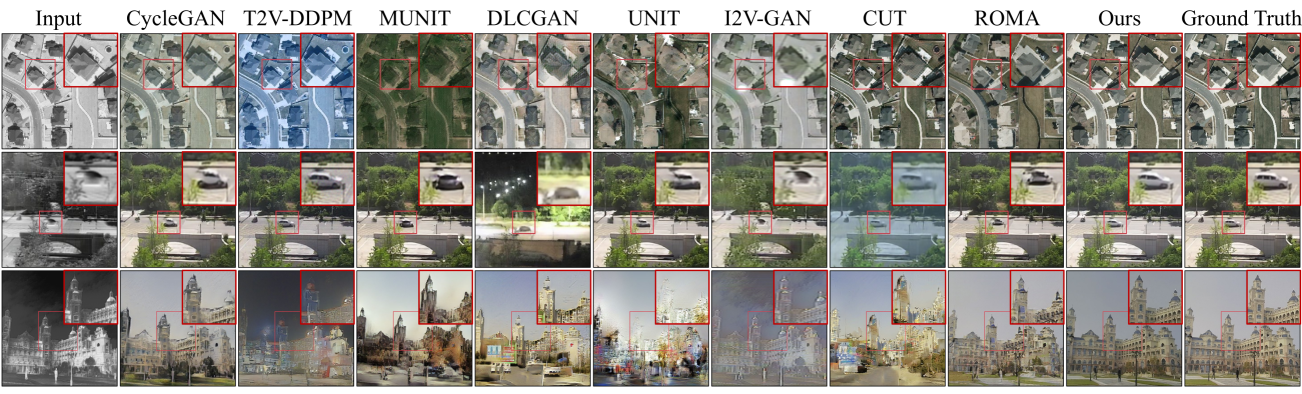
Figure 3: Qualitative results of CM-Diff for the infrared-to-visible image translation task. The first row corresponds to the VEDAI dataset, the second row to the AVIID dataset, and the third row to the $\text{M}^{3}\text{FD}$ dataset.

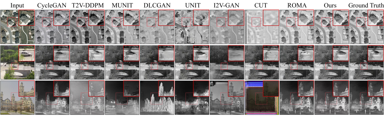
Figure 4: Qualitative results of CM-Diff for the visible-to-infrared image translation task.

4.1 Comparison with State-of-the-Art Methods

1) Quantitative Results: The quantitative comparison results are listed in Table 1. The evaluation metrics include FID [14], SSIM [41], LPIPS [46], and PSNR for both the infrared-to-visible image translation task and the visible-to-infrared image translation task. Overall, our method demonstrates superior performance compared to unidirectional and bidirectional modality translation methods.

Compared to the DDPM-based method T2V-DDPM [32], the proposed method achieves a 7.44% improvement in PSNR, along with a 64.04% reduction in FID for the infrared-to-visible image translation task on the AVIID [11] dataset. On the $\text{M}^{3}\text{FD}$ [25] dataset, the enhancements are also pronounced, with a 53.04% increase in PSNR and a 56.29% reduction in LPIPS. This improvement stems from the limitations of diffusion-based unidirectional methods, which focus solely on learning the data distribution in the target modality and establishing mappings within it, thereby missing deeper semantic connections. In contrast, BDT can simultaneously learn the data distributions of both modalities. Additionally, the CFC is utilized to enhance the semantic guidance of the source modality image.

Compared to GAN-based unidirectional translation methods, our proposed method achieves improvements across the three datasets. On the AVIID[11] dataset, for the infrared-to-visible image translation task, FID decreases by 72.20% and PSNR increases by 48.88% compared to CUT [35], while FID decreases by 31.88% and PSNR increases by 23.93% compared to ROMA [44]. This improvement can be attributed to the proposed DDPM-based method, which transforms the data distribution into a series of noise distributions to avoid the problem of mode collapse. Additionally, it employs SCI during the sampling phase to incorporate observed statistical information, thereby improving the consistency between the generated results and the real data distribution.

Compared to GAN-based bidirectional translation methods, our proposed method also demonstrates performance gains. On the AVIID[11] dataset, for the infrared-to-visible image translation task, PSNR increases by 1.41% compared to MUNIT [16]. The observed improvement can be ascribed to the adoption of a BDT, which effectively encodes directional embeddings and edge information while leveraging multi-scale features extracted by the source modality encoder. This method mitigates modality distribution ambiguity arising from the structural and semantic similarities between infrared and visible images.

2) Qualitative Results: We compare the infrared-to-visible (Fig. 3) and visible-to-infrared (Fig. 4) translation results of state-of-the-art methods with our approach. In the first row, using the VEDAI [36] dataset, we observe that all methods transfer semantic information well, but our method outperforms DCLGAN [10] and UNIT [27] in terms of color and detail. This is due to the limitations of DCLGAN and UNIT in accurately defining object boundaries and utilizing spatial information. In the second row (AVIID [11] dataset), methods like CycleGAN [48], MUNIT [16], and ROMA [44] produce blurred or distorted objects. While CUT [35], T2V-DDPM [32], and our method generate clearer object structures, our method stands out by improving color fidelity through inference guidance with the SCI. The third row shows challenging samples with complex backgrounds and pedestrians. Methods like T2V-DDPM [32] and CUT [35] tend to mistakenly render background buildings as sky. In contrast, our method accurately reconstructs architectural details and sky backgrounds, thanks to the CFC module that ensures precise feature generation and noise control.

4.2 Ablation Study

We conduct ablation studies to analyze the effectiveness of each proposed novel component:

1) Effect of CFC: We conducted ablation experiments to demonstrate the effectiveness of the source modality features and edge feature map cues in preserving content consistency in translation results. The quantitative results are presented in Table. 2. It can be observed that the removal of the modality encoders and the edge detection part leads to a notable drop in the overall performance in both translation directions. We can see that external control using modality and edge features can effectively help the network distinguish boundaries of objects in the image.

Table 2: Effect of CFC.

CFC	infrared $\rightarrow$ visible				visible $\rightarrow$ infrared
	PSNR$\uparrow$	SSIM$\uparrow$	LPIPS$\downarrow$	FID$\downarrow$	PSNR$\uparrow$	SSIM$\uparrow$	LPIPS$\downarrow$	FID$\downarrow$
w/	19.89	0.774	0.185	94.11	24.06	0.883	0.096	46.18
w/o	19.17	0.761	0.201	101.13	24.05	0.880	0.098	47.84

2) Effect of TDG: In Table 3, we investigate the impact of TDG on the quality of translation results for the two directions. When direction labels are passed through the label embedding layer and used to guide the network, the PSNR and SSIM metrics for the infrared-to-visible image translation task improve by 7.16% and 6.91%, respectively. Similarly, for the visible-to-infrared translation task, these metrics increase by 5.29% and 14.52%, respectively. These results demonstrate that TDG is indispensable during training, as it helps the model recognize noisy data and provide crucial guidance. Moreover, during inference, the TDG corresponds to assisting the model in executing the correct translation direction, further highlighting its importance.

Table 3: Effect of TDG.

TDG	infrared $\rightarrow$ visible				visible $\rightarrow$ infrared
	PSNR$\uparrow$	SSIM$\uparrow$	LPIPS$\downarrow$	FID$\downarrow$	PSNR$\uparrow$	SSIM$\uparrow$	LPIPS$\downarrow$	FID$\downarrow$
w/	19.89	0.774	0.185	94.11	24.06	0.883	0.096	46.18
w/o	18.56	0.724	0.253	142.79	22.85	0.771	0.181	163.87

3) Effect of SCI: Several ablation experiments are conducted to demonstrate the efficacy of our SCI. As listed in Table 4, in the infrared-to-visible image translation task, the $\mathcal{L}_{scl}$ plays a significant role in enhancing modality translation performance, resulting in an improvement of 5.85% in PSNR and 1.57% in SSIM compared to the case without SCI. In the visible-to-infrared image translation task, it results in an improvement of 52.70% in PSNR, 5.87% in SSIM, 26.15% in LPIPS, and 19.97% in FID. Moreover, in the visible-to-infrared image translation task, incorporating the $\mathcal{L}_{ccl}$ further boosts the model’s performance, leading to an improvement of 0.16% in PSNR and 0.21% in FID.

Table 4: Effect of SCI.

$\mathcal{L}_{{ccl}}$	$\mathcal{L}_{{scl}}$	infrared $\rightarrow$ visible				visible $\rightarrow$ infrared
		PSNR$\uparrow$	SSIM$\uparrow$	LPIPS$\downarrow$	FID$\downarrow$	PSNR$\uparrow$	SSIM$\uparrow$	LPIPS$\downarrow$	FID$\downarrow$
✓	✓	19.89	0.774	0.185	94.11	24.06	0.883	0.096	46.18
×	✓	19.88	0.774	0.185	93.65	24.02	0.883	0.096	46.28
✓	×	19.54	0.775	0.201	97.39	15.64	0.840	0.129	56.88
×	×	18.78	0.762	0.205	105.02	15.73	0.834	0.130	57.83

5 Conclusion

This paper introduces CM-Diff, a unified framework that utilizes DDPM for bidirectional translation between infrared and visible images. Our approach leverages the diffusion model and incorporates a Bidirectional Diffusion Training (BDT) strategy to distinguish and learn modality-specific data distributions while establishing robust bidirectional mappings. We have also proposed a Statistical Constraint Inference (SCI) strategy for maintaining consistency between the statistical distributions of the translated images and training images. Extensive experiments have shown the effectiveness of our method.

CM-Diff: A Single Generative Network for Bidirectional Cross-Modality Translation Diffusion Model Between Infrared and Visible Images (Supplementary Material)

In the supplementary materials, Section A evaluates the effectiveness of the Statistical Constraint Inference (SCI) strategy using a pixel intensity frequency histogram analysis. Section B presents a detailed ablation study on the constraint scale factor. Section C reports the validation results of translation outcomes from different modality translation methods in the object detection task. In Section D, we provide additional translation results for complex scenes from the $\text{M}^{3}\text{FD}$, AVIID and VEDAI datasets, along with an analysis of variations in different loss functions during the training process. Section E further discusses the results of the ablation study. Section F outlines the experimental implementation. Finally, sections G and H detail the evaluation metrics and datasets used in the experiments, respectively.

Appendix A Analysis of Statistical Constraint Inference

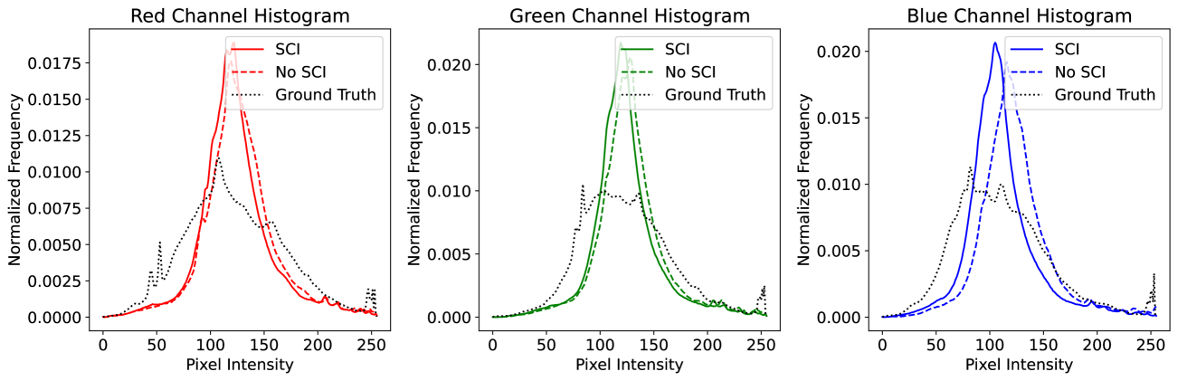
Figure 5: Comparison of histograms for each channel of visible images. The distribution of the images obtained using SCI, without SCI, and the ground truth visible images are presented.

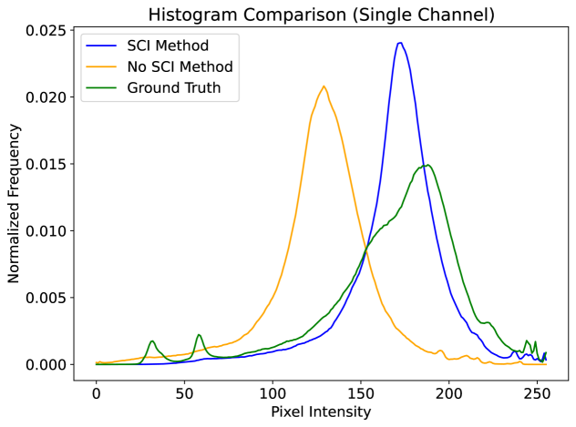
Figure 6: Comparison of histograms for infrared images. The distribution of the images obtained using SCI, without SCI, and the ground truth visible images are presented.

As shown in Fig. 5, the infrared-to-visible translation results using the Statistical Constraint Inference (SCI) strategy exhibit a shift in the frequency peak of each channel towards lower pixel intensity values, particularly noticeable in the blue and green channels. The reduction in abnormal pixel intensity values significantly decreases the occurrence of color artifacts in the translated visible images. This is also clearly reflected in the visible-to-infrared translation results. As shown in Fig. 6, the translation results using the SCI strategy are more consistent with the ground truth histogram distribution.

This demonstrates that the translated images generated using the SCI strategy exhibit a distribution that is closer to the real distribution, while also avoiding the color anomalies introduced by the Bidirectional Diffusion Training (BDT) strategy. Consequently, CM-Diff achieves high-quality cross-modality translation between infrared and visible images within a single-generation network.

Appendix B Analysis of the Constraint Scale Factor

Table 5: Effect of the Constraint Scale Factors. The best performance for each metric is highlighted in bold.

$\lambda_{{ccl}},\lambda_{{scl}}$	infrared $\rightarrow$ visible
	PSNR$\uparrow$	SSIM$\uparrow$	LPIPS$\downarrow$	FID$\downarrow$
0	18.78	0.762	0.205	105.02
10	19.88	0.775	0.186	93.66
20	19.89	0.774	0.185	94.11
40	19.85	0.774	0.185	93.74
60	19.84	0.774	0.185	93.68
$\lambda_{{ccl}},\lambda_{{scl}}$	visible $\rightarrow$ infrared
	PSNR$\uparrow$	SSIM$\uparrow$	LPIPS$\downarrow$	FID$\downarrow$
0	15.73	0.834	0.130	57.83
10	22.78	0.879	0.099	47.18
20	24.06	0.883	0.096	46.18
40	24.13	0.883	0.095	46.01
60	24.10	0.883	0.096	45.98

We conducted several ablation experiments to assess the impact of the constraint scale factor value. As shown in Table 5, we evaluated the modality translation performance using varying values of the constraint scale factor. As the values of $\lambda_{\text{ccl}}$ and $\lambda_{\text{scl}}$ increased, PSNR, SSIM, LPIPS, and FID all tended to improve. Notably, when $\lambda_{\text{ccl}},\lambda_{\text{scl}}=20$, we achieved the highest PSNR (19.89) and LPIPS (0.185) in the infrared-to-visible image translation task, and the highest SSIM (0.883) in the visible-to-infrared image translation task. However, increasing the constraint scale factor values from 40 to 60 led to a slight performance drop in PSNR by 0.12% and LPIPS by 0.11% in the visible-to-infrared image translation task. This drop is attributed to overly constraining the mean of the sampling process, which weakened the model’s ability to handle underlying noise or randomness.

Appendix C Analysis of Generated Data in Object Detection Applications

Table 6: Quantitative evaluation of visible-to-infrared image translation performance of various translation methods based on CFINet.

Method	P	R	$mAP_{50}$	$mAP_{75}$	$mAP$
ROMA [44]	0.133	0.027	0.036	0.022	0.012
CUT [35]	0.418	0.157	0.187	0.159	0.082
I2V-GAN [22]	0.379	0.113	0.179	0.144	0.077
Ground Truth	0.471	0.368	0.449	0.306	0.168
Ours	0.313	0.198	0.281	0.249	0.138

Table 7: Quantitative evaluation of infrared-to-visible image translation performance of various translation methods based on CFINet.

Method	P	R	$mAP_{50}$	$mAP_{75}$	$mAP$
ROMA [44]	0.240	0.106	0.175	0.136	0.072
CUT [35]	0.185	0.025	0.068	0.059	0.032
I2V-GAN [22]	0.168	0.079	0.129	0.090	0.048
Ground Truth	0.237	0.179	0.386	0.217	0.121
Ours	0.241	0.165	0.265	0.206	0.105

We employ the recent small object detection method, CFINet [45], and train it separately on infrared and visible data using the VEDAI dataset. Various translation methods are utilized to perform infrared-to-visible and visible-to-infrared modality translation. The translation results are then evaluated using CFINet . For comparison, we selected several high-performing modality translation methods, including ROMA [44], CUT [35], and I2V-GAN [22]. The quantitative results for the infrared and visible modalities are shown in Tables 6 and 7, respectively.

In the comparison of infrared modality translation results, significant differences can be observed in terms of precision (P), recall (R), and mean average precision (mAP). As shown in the table, the Ground Truth achieves the best performance, with the highest precision (0.471) and recall (0.368). It also attains the highest mAP values, including mAP₅₀ = 0.449, mAP₇₅ = 0.306, and an overall mAP of 0.168. Among the modality translation methods, our approach demonstrates the best performance, achieving mAP₅₀, mAP₇₅, and overall mAP values of 0.281, 0.249, and 0.138, respectively. These results are significantly superior to those of ROMA, CUT, and I2V-GAN. Additionally, our method exhibits a recall of 0.198, which is substantially higher than that of other approaches, indicating its effectiveness in the object detection task. Regarding the other modality translation methods, CUT and I2V-GAN perform similarly in terms of precision and mAP, though CUT consistently achieves slightly better results. In contrast, ROMA exhibits the weakest performance across all metrics, suggesting that its translated infrared images contribute minimally to the detection task. In summary, our method generates higher-quality infrared images and substantially improves the performance of object detection tasks.

In the comparison of visible modality translation results, significant differences can be observed in terms of precision (P), recall (R), and mean average precision (mAP). As shown in the table, the Ground Truth achieves the best performance, with relatively high precision (0.237) and recall (0.179). It also attains the highest mAP values, including mAP₅₀ = 0.386, mAP₇₅ = 0.217, and an overall mAP of 0.121. Among the modality translation methods, our approach demonstrates superior performance compared to others. Specifically, it achieves mAP₅₀, mAP₇₅, and overall mAP values of 0.265, 0.206, and 0.105, respectively, significantly outperforming ROMA, CUT, and I2V-GAN. Additionally, our method exhibits a recall of 0.165, second only to the Ground Truth, indicating its effectiveness in the object detection task under the visible modality. Regarding other translation methods, ROMA performs relatively well in terms of precision and mAP but has a lower recall (0.106) compared to our model. CUT and I2V-GAN demonstrate weaker overall performance, with CUT exhibiting the lowest scores across all metrics, suggesting that its translated visible images are of lower quality and less beneficial for object detection tasks. In summary, our method generates higher-quality visible images and achieves superior performance in object detection tasks.

Finally, we observe that the quality of our infrared translation results is superior to that of visible translation results, both in terms of translation quality and object detection task performance. This observation is also supported by the training loss depicted in Fig. 7, where the loss for visible-to-infrared translation is consistently lower than that for infrared-to-visible translation. This phenomenon can be attributed to the inherent characteristics of infrared and visible images. Specifically, visible images consist of three channels representing the intensity values of red, green, and blue, whereas infrared images contain only a single channel reflecting infrared radiation intensity.

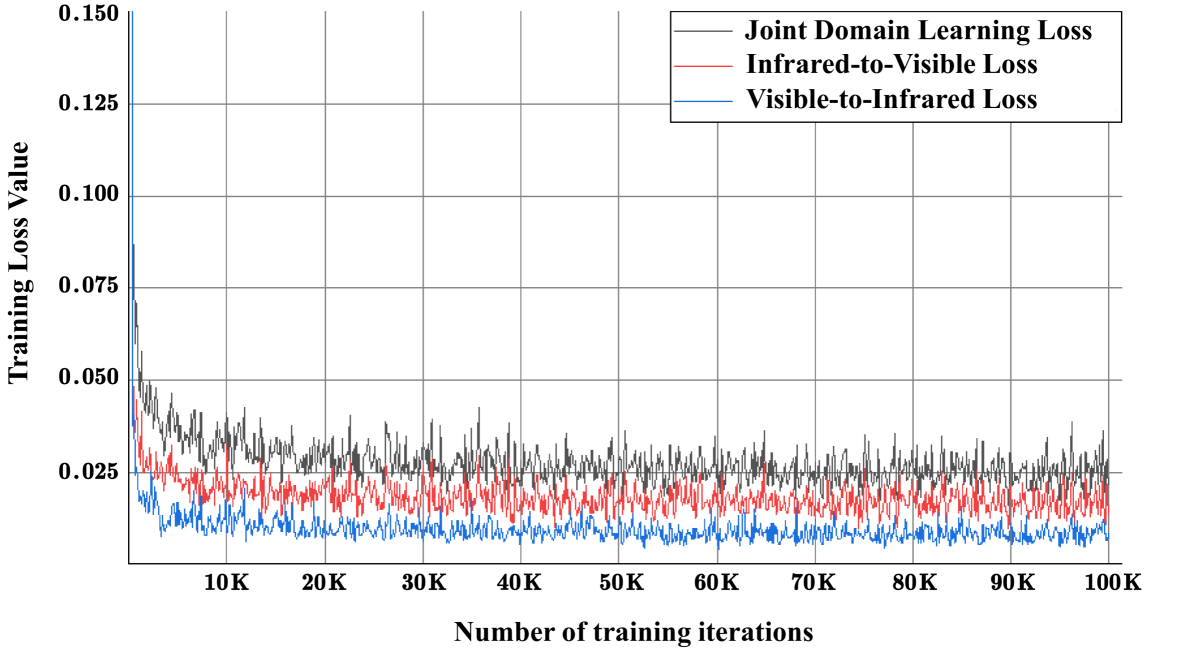
Figure 7: The training loss evolves with the number of iterations. Due to the significant fluctuations in the loss values of individual iterations, which make it challenging to discern overall trends, we instead utilize the average loss value over an entire training epoch and use the iteration count as the horizontal axis.

Appendix D More Translation Results

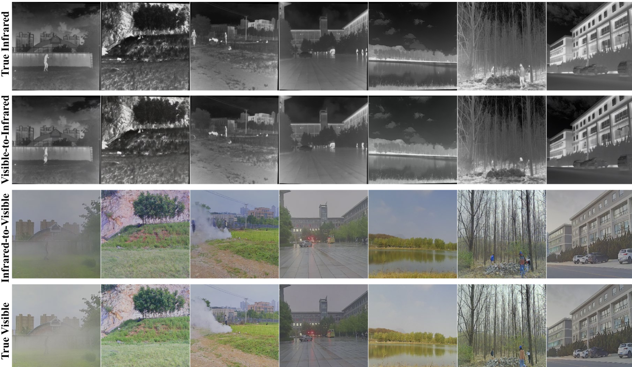
Figure 8: Modality translation results on the $\text{M}^{3}\text{FD}$ dataset. The first row represents real infrared images, the second and third rows show generated infrared and visible images, respectively, and the fourth row represents real visible images.

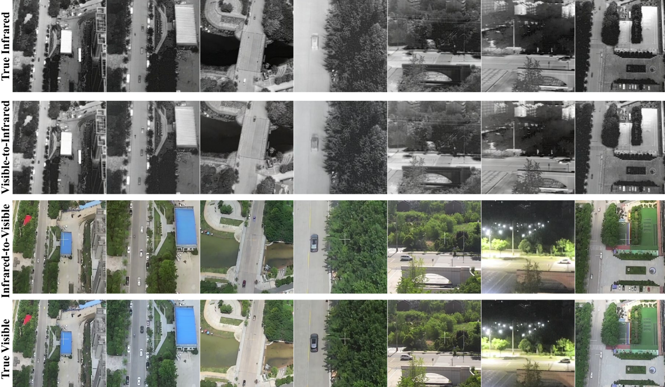
Figure 9: Modality translation results on the AVIID dataset. The first row represents real infrared images, the second and third rows show generated infrared and visible images, respectively, and the fourth row represents real visible images.

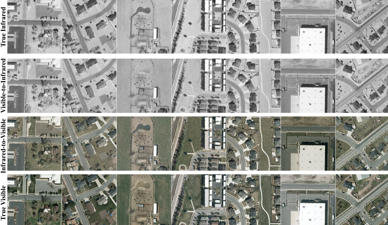
Figure 10: Modality translation results on the VEDAI dataset. The first row represents real infrared images, the second and third rows show generated infrared and visible images, respectively, and the fourth row represents real visible images.

As shown in Figs. 8, 9, and 10, additional translation results on the $\text{M}^{3}\text{FD}$, AVIID, and VEDAI datasets are presented. In these figures, the first and fourth rows represent the real infrared and visible images, respectively. The second and third rows correspond to the translated infrared and visible images, generated using the visible and infrared images as conditions, respectively. These images encompass complex scenes such as urban areas, wilderness, forests, and lakes. The results demonstrate that CM-Diff exhibits strong modality translation capabilities even in complex outdoor environments.

Figure 11: Comparisons of different ablation studies for the visible-to-infrared image translation task. We evaluate the impact of the Statistical Constraint Inference (SCI), which consists of $\mathcal{L}_{{ccl}}$ and $\mathcal{L}_{{scl}}$, the Cross-modality Feature Control (CFC) component, and the translation direction guidance (TDG).

Appendix E Visualization of the Ablation Study Results

To further explain how each novel component affects the results of our proposed method on tasks infrared-to-visible and visible-to-infrared image translation, we provide the visual translation results of various ablation experiments on the VEDAI [36] dataset for these two image translation tasks in Fig. 11. We can observe that in the image translation tasks in both directions, the visualization results of the second, fourth, and fifth columns lack the observed statistical information to constrain the sampling process, resulting in obvious color anomalies. On the contrary, the seventh column of Fig. 11 shows that our proposed method uses cross-modality feature control and statistical constraint to achieve color and detail performance close to real visible and infrared images. Additionally, in the results shown in the seventh column of Fig. 11, noticeable object blurriness and unclear boundaries can be observed. This further demonstrates the effectiveness of direction label guidance.

Appendix F Implementation Details

To effectively integrate feature information, we incorporate a cross-modality attention mechanism with 64 channels at feature map resolutions of 8, 16, and 32 during both the upsampling and downsampling processes. Furthermore, edge details are extracted from both the infrared and visible images using a pre-trained DexiNed model. For training and evaluation, all images in the datasets are resized to a resolution of $256\times 256$. The U-Net architecture employs a base channel dimension of 128 across all datasets. During training, the learning rate is initialized to $1\times 10^{-4}$ and reduced by 90% every 2,000 iterations. We utilize the AdamW optimizer with a batch size of 6, and the training process is conducted over 100,000 iterations. To enhance the precision of the translation results, we modify the original noise schedule by reducing $\beta_{T}$ from 0.02 to 0.01. This adjustment decreases the intensity of added noise, thereby promoting more accurate feature mapping and minimizing noise-induced artifacts. Specifically, the noise schedule is defined such that $\beta_{t}$ increases linearly from $\beta_{1}=0.0001$ to $\beta_{T}=0.01$. Considering the symmetric nature of the relationship between the infrared and visible data modalities, the weighting factors $\lambda_{\text{{ir}-to-{vis}}}$ and $\lambda_{\text{{vis}-to-{ir}}}$ are both set to 1.0, despite the lower learning difficulty in the infrared modality. During the generation phase, we employ $T=1,000$ steps with two constraint scale correction factors. Both $\lambda_{{ccl}}$ and $\lambda_{{scl}}$ are set to 20.0 to ensure superior generative detail. All experiments are performed on a system equipped with an Intel(R) Xeon(R) CPU E5-2698 v4 @ 2.20GHz and four NVIDIA V100 GPUs.

Appendix G Metrics

To objectively evaluate the effectiveness of our method, we employ four commonly used image quality assessment metrics to evaluate our model.

The Frechet Inception Distance Score (FID)[14] measures the similarity between the distribution of generated images and that of real images. The FID calculation is expressed as follows:

$$\text{FID}(v^{\prime},v)=\|\mu_{v}-\mu_{v}^{\prime}\|^{2}+\operatorname{tr}(\Sigma_{v}+\Sigma_{v^{\prime}}-2(\Sigma_{v}\cdot\Sigma_{v^{\prime}})^{\frac{1}{2}}),$$ (15)

where $\mu_{v}$ and $\mu_{v^{\prime}}$ are the element-wise means of the feature vectors of all real and translated images, respectively, and $\Sigma_{v},\Sigma_{v^{\prime}}$ are the corresponding covariance matrices of these feature vectors, extracted by the Inception-V3 network.

The Structural Similarity Index Measure (SSIM)[41] evaluates the quality of translated images by considering their luminance, contrast, and structural similarity to the real images. The SSIM calculation is expressed as follows:

$$\text{SSIM}(v^{\prime},v)=\frac{\left(2\mu_{v}\cdot\mu_{v^{\prime}}+{c}_{1}\right)\left(\sigma_{v}\cdot\sigma_{v^{\prime}}+{c}_{2}\right)}{\left(\mu_{v}^{2}+\mu_{v^{\prime}}^{2}+{c}_{1}\right)\left(\sigma_{v}^{2}+\sigma_{v^{\prime}}^{2}+{c}_{2}\right)},$$ (16)

where $\mu_{v}$ and $\mu_{v^{\prime}}$ denote the mean values of the reference image and the translated image, respectively, while $\sigma_{v}$ and $\sigma_{v^{\prime}}$ represent their corresponding standard deviations.

The Learned Perceptual Image Patch Similarity (LPIPS) [46] measures the similarity between the feature vectors of reference and translated images. To compute this metric, features at various layers are extracted using AlexNet [20]. The LPIPS calculation is expressed as follows:

$$\text{LPIPS}(v^{\prime},v)=\sum\limits_{i}^{I}\sum\limits_{h_{i},w_{i}}\frac{\omega_{i}\cdot\left[f_{i}(v^{\prime})_{h_{i},w_{i}}-f_{i}(v)_{h_{i},w_{i}}\right]^{2}}{{H}_{i}\cdot{W}_{i}},$$ (17)

where $f_{i}(v^{\prime}),f_{i}(v)\in\mathbb{R}^{H_{i}\times W_{i}\times i}$ represents the features extracted from the $i$-th layer of AlexNet. $\omega_{i}$ represents the weight of the feature distance at the $i$-th layer, used to adjust the contribution of different layer features to the overall perceptual similarity.

The Peak Signal-to-Noise Ratio (PSNR) measures the quality of generated images by calculating the mean squared error (MSE) between the real and generated images and representing it as a signal-to-noise ratio. The PSNR calculation is expressed as follows:

$$\text{PSNR}(v^{\prime},v)=10\log_{10}\frac{M\cdot N\cdot{INTENSITY}_{max}^{2}}{\sum\limits_{i=1}^{M}\sum\limits_{j=1}^{{n}}[v_{ij}-v^{\prime}_{ij}]^{2}},$$ (18)

where ${INTENSITY}_{max}$ represents the maximum possible pixel value in the image. In our case, the images are 8-bit, meaning the maximum possible pixel value is $(2^{8}-1)$.

Appendix H Datasets

The VEDAI dataset [36], designed for dual-modality small vehicle detection in aerial imagery, comprises 1,209 paired infrared-visible images with resolutions of $1024\times 1024$ and $512\times 512$. Featuring near-infrared imagery, it supports dual-modality detection tasks with diverse targets, backgrounds, and small-object scenarios. Comprehensive ground-truth annotations enable robust algorithm development and benchmarking. In our experimental setup, 1,089 image pairs are allocated for training, and 120 pairs are reserved for testing to ensure a balanced evaluation.

The AVIID dataset [11] comprises paired images captured by a dual-light camera on a UAV under varying conditions. It is divided into three subsets: AVIID-1, which contains 993 pairs of $434\times 434$ images of roads and common vehicles; AVIID-2, consisting of 1,090 pairs of $434\times 434$ low-light images with noise and blur; and AVIID-3, which includes 1,280 pairs of $512\times 512$ images with diverse scenes, such as roads, bridges, and residential streets. While originally created for the visible-to-infrared image translation task, our method supports the bidirectional cross-modality translation task, including the infrared-to-visible image task. For our experiments, the dataset is split into 2,674 training pairs and 669 testing pairs.

The $\text{M}^{3}\text{FD}$ dataset [25] contains 4,500 registered visible-infrared image pairs with a resolution of $1024\times 768$ pixels. Originally created for multi-sensor fusion and object detection, it is also suitable for image-to-image translation tasks, despite minor misalignments. The dataset includes scenes from Dalian University of Technology, Golden Stone Beach, and Jinzhou District in Dalian, China. We split the dataset into 3,780 pairs for training and 210 pairs for testing.

References

- Aslahishahri et al. [2021] Masoomeh Aslahishahri, Kevin G Stanley, Hema Duddu, Steve Shirtliffe, Sally Vail, Kirstin Bett, Curtis Pozniak, and Ian Stavness. From rgb to nir: Predicting of near infrared reflectance from visible spectrum aerial images of crops. In Proceedings of the IEEE/CVF international conference on computer vision, pages 1312–1322, 2021.
- Boroujeni and Razi [2024] Sayed Pedram Haeri Boroujeni and Abolfazl Razi. Ic-gan: An improved conditional generative adversarial network for rgb-to-ir image translation with applications to forest fire monitoring. Expert Systems with Applications, 238:121962, 2024.
- Deng et al. [2021] Fuqin Deng, Hua Feng, Mingjian Liang, Hongmin Wang, Yong Yang, Yuan Gao, Junfeng Chen, Junjie Hu, Xiyue Guo, and Tin Lun Lam. Feanet: Feature-enhanced attention network for rgb-thermal real-time semantic segmentation. In 2021 IEEE/RSJ international conference on intelligent robots and systems (IROS), pages 4467–4473. IEEE, 2021.
- Dhariwal and Nichol [2021] Prafulla Dhariwal and Alexander Nichol. Diffusion models beat gans on image synthesis. Advances in neural information processing systems, 34:8780–8794, 2021.
- Di et al. [2019] Xing Di, Benjamin S Riggan, Shuowen Hu, Nathaniel J Short, and Vishal M Patel. Polarimetric thermal to visible face verification via self-attention guided synthesis. In 2019 International Conference on Biometrics (ICB), pages 1–8. IEEE, 2019.
- Ding et al. [2025] Jiangang Ding, Yiquan Du, Wei Li, Lili Pei, and Ningning Cui. Lg-diff: Learning to follow local class-regional guidance for nearshore image cross-modality high-quality translation. Information Fusion, 117:102870, 2025.
- Endres and Schindelin [2003] Dominik Maria Endres and Johannes E Schindelin. A new metric for probability distributions. IEEE Transactions on Information theory, 49(7):1858–1860, 2003.
- Fu et al. [2023] Haolong Fu, Shixun Wang, Puhong Duan, Changyan Xiao, Renwei Dian, Shutao Li, and Zhiyong Li. Lraf-net: Long-range attention fusion network for visible–infrared object detection. IEEE Transactions on Neural Networks and Learning Systems, 2023.
- Guo et al. [2024] Junjie Guo, Chenqiang Gao, Fangcen Liu, Deyu Meng, and Xinbo Gao. Damsdet: Dynamic adaptive multispectral detection transformer with competitive query selection and adaptive feature fusion. ECCV, 2024.
- Han et al. [2021] Junlin Han, Mehrdad Shoeiby, Lars Petersson, and Mohammad Ali Armin. Dual contrastive learning for unsupervised image-to-image translation. In Proceedings of the IEEE/CVF conference on computer vision and pattern recognition, pages 746–755, 2021.
- Han et al. [2023] Zonghao Han, Ziye Zhang, Shun Zhang, Ge Zhang, and Shaohui Mei. Aerial visible-to-infrared image translation: dataset, evaluation, and baseline. Journal of Remote Sensing, 3:0096, 2023.
- Han et al. [2024a] Zonghao Han, Shun Zhang, Yuru Su, Xiaoning Chen, and Shaohui Mei. Dr-avit: Towards diverse and realistic aerial visible-to-infrared image translation. IEEE Transactions on Geoscience and Remote Sensing, 2024a.
- Han et al. [2024b] Zonghao Han, Shun Zhang, Yuru Su, Xiaoning Chen, and Shaohui Mei. Dr-avit: Towards diverse and realistic aerial visible-to-infrared image translation. IEEE Transactions on Geoscience and Remote Sensing, 2024b.
- Heusel et al. [2017] Martin Heusel, Hubert Ramsauer, Thomas Unterthiner, Bernhard Nessler, and Sepp Hochreiter. Gans trained by a two time-scale update rule converge to a local nash equilibrium. Advances in neural information processing systems, 30, 2017.
- Ho et al. [2020] Jonathan Ho, Ajay Jain, and Pieter Abbeel. Denoising diffusion probabilistic models. Advances in neural information processing systems, 33:6840–6851, 2020.
- Huang et al. [2018] Xun Huang, Ming-Yu Liu, Serge Belongie, and Jan Kautz. Multimodal unsupervised image-to-image translation. In Proceedings of the European conference on computer vision (ECCV), pages 172–189, 2018.
- Isola et al. [2017] Phillip Isola, Jun-Yan Zhu, Tinghui Zhou, and Alexei A Efros. Image-to-image translation with conditional adversarial networks. In Proceedings of the IEEE conference on computer vision and pattern recognition, pages 1125–1134, 2017.
- Ji et al. [2023] Wei Ji, Jingjing Li, Cheng Bian, Zongwei Zhou, Jiaying Zhao, Alan L Yuille, and Li Cheng. Multispectral video semantic segmentation: A benchmark dataset and baseline. In Proceedings of the IEEE/CVF Conference on Computer Vision and Pattern Recognition, pages 1094–1104, 2023.
- Koller and Friedman [2009] Daphne Koller and Nir Friedman. Probabilistic graphical models: principles and techniques. MIT press, 2009.
- Krizhevsky et al. [2012] Alex Krizhevsky, Ilya Sutskever, and Geoffrey E Hinton. Imagenet classification with deep convolutional neural networks. Advances in neural information processing systems, 25, 2012.
- Li et al. [2023] Qing Li, Changqing Zhang, Qinghua Hu, Pengfei Zhu, Huazhu Fu, and Lei Chen. Stabilizing multispectral pedestrian detection with evidential hybrid fusion. IEEE Transactions on Circuits and Systems for Video Technology, 2023.
- Li et al. [2021] Shuang Li, Bingfeng Han, Zhenjie Yu, Chi Harold Liu, Kai Chen, and Shuigen Wang. I2v-gan: Unpaired infrared-to-visible video translation. In Proceedings of the 29th ACM international conference on multimedia, pages 3061–3069, 2021.
- Lin et al. [2024] Jingyu Lin, Guiqin Zhao, Jing Xu, Guoli Wang, Zejin Wang, Antitza Dantcheva, Lan Du, and Cunjian Chen. Difftv: Identity-preserved thermal-to-visible face translation via feature alignment and dual-stage conditions. In Proceedings of the 32nd ACM International Conference on Multimedia, pages 10930–10938, 2024.
- Liu et al. [2024] Fangcen Liu, Chenqiang Gao, Yaming Zhang, Junjie Guo, Jinhao Wang, and Deyu Meng. Infmae: A foundation model in infrared modality. ECCV, 2024.
- Liu et al. [2022] Jinyuan Liu, Xin Fan, Zhanbo Huang, Guanyao Wu, Risheng Liu, Wei Zhong, and Zhongxuan Luo. Target-aware dual adversarial learning and a multi-scenario multi-modality benchmark to fuse infrared and visible for object detection. In Proceedings of the IEEE/CVF Conference on Computer Vision and Pattern Recognition, pages 5802–5811, 2022.
- Liu et al. [2023] Jinyuan Liu, Zhu Liu, Guanyao Wu, Long Ma, Risheng Liu, Wei Zhong, Zhongxuan Luo, and Xin Fan. Multi-interactive feature learning and a full-time multi-modality benchmark for image fusion and segmentation. In Proceedings of the IEEE/CVF international conference on computer vision, pages 8115–8124, 2023.
- Liu et al. [2017] Ming-Yu Liu, Thomas Breuel, and Jan Kautz. Unsupervised image-to-image translation networks. Advances in neural information processing systems, 30, 2017.
- Liu et al. [2018] Shuo Liu, Vijay John, Erik Blasch, Zheng Liu, and Ying Huang. Ir2vi: Enhanced night environmental perception by unsupervised thermal image translation. In Proceedings of the IEEE Conference on Computer Vision and Pattern Recognition Workshops, pages 1153–1160, 2018.
- Luo et al. [2022] Fuya Luo, Yunhan Li, Guang Zeng, Peng Peng, Gang Wang, and Yongjie Li. Thermal infrared image colorization for nighttime driving scenes with top-down guided attention. IEEE Transactions on Intelligent Transportation Systems, 23(9):15808–15823, 2022.
- Ma et al. [2024] Decao Ma, Shaopeng Li, Juan Su, Yong Xian, and Tao Zhang. Visible-to-infrared image translation for matching tasks. IEEE Journal of Selected Topics in Applied Earth Observations and Remote Sensing, 2024.
- [31] Rahman Maqsood, Fazeel Abid, et al. Cycle consistency and fine-grained image to image translation in augmentation: An overview.
- Nair and Patel [2023] Nithin Gopalakrishnan Nair and Vishal M Patel. T2v-ddpm: Thermal to visible face translation using denoising diffusion probabilistic models. In 2023 IEEE 17th International Conference on Automatic Face and Gesture Recognition (FG), pages 1–7. IEEE, 2023.
- Oliveira et al. [2024] Guilherme C Oliveira, Quoc C Ngo, João P Papa, and Dinesh Kumar. A stable diffusion approach for rgb to thermal image conversion for leg ulcer assessment. In 2024 IEEE 37th International Symposium on Computer-Based Medical Systems (CBMS), pages 158–163. IEEE, 2024.
- Ordun et al. [2023] Catherine Ordun, Edward Raff, and Sanjay Purushotham. When visible-to-thermal facial gan beats conditional diffusion. In 2023 IEEE International Conference on Image Processing (ICIP), pages 181–185. IEEE, 2023.
- Park et al. [2020] Taesung Park, Alexei A Efros, Richard Zhang, and Jun-Yan Zhu. Contrastive learning for unpaired image-to-image translation. In Computer Vision–ECCV 2020: 16th European Conference, Glasgow, UK, August 23–28, 2020, Proceedings, Part IX 16, pages 319–345. Springer, 2020.
- Razakarivony and Jurie [2016] Sebastien Razakarivony and Frederic Jurie. Vehicle detection in aerial imagery: A small target detection benchmark. Journal of Visual Communication and Image Representation, 34:187–203, 2016.
- Ren et al. [2023] Kan Ren, Wenjing Zhao, Guohua Gu, and Qian Chen. Eads: Edge-assisted and dual similarity loss for unpaired infrared-to-visible video translation. Infrared Physics & Technology, 134:104936, 2023.
- Sasaki et al. [2021] Hiroshi Sasaki, Chris G Willcocks, and Toby P Breckon. Unit-ddpm: Unpaired image translation with denoising diffusion probabilistic models. arXiv preprint arXiv:2104.05358, 2021.
- Soria et al. [2023] Xavier Soria, Angel Sappa, Patricio Humanante, and Arash Akbarinia. Dense extreme inception network for edge detection. Pattern Recognition, 139:109461, 2023.
- Wang et al. [2024] Haining Wang, Na Li, Huijie Zhao, Yan Wen, Yi Su, and Yuqiang Fang. Mappingformer: Learning cross-modal feature mapping for visible-to-infrared image translation. In Proceedings of the 32nd ACM International Conference on Multimedia, pages 10745–10754, 2024.
- Wang et al. [2004] Zhou Wang, Alan C Bovik, Hamid R Sheikh, and Eero P Simoncelli. Image quality assessment: from error visibility to structural similarity. IEEE transactions on image processing, 13(4):600–612, 2004.
- Yadav et al. [2023] Nand Kumar Yadav, Satish Kumar Singh, and Shiv Ram Dubey. Tva-gan: attention guided generative adversarial network for thermal to visible image transformations. Neural Computing and Applications, 35(27):19729–19749, 2023.
- Yang et al. [2023] Ling Yang, Zhilong Zhang, Yang Song, Shenda Hong, Runsheng Xu, Yue Zhao, Wentao Zhang, Bin Cui, and Ming-Hsuan Yang. Diffusion models: A comprehensive survey of methods and applications. ACM Computing Surveys, 56(4):1–39, 2023.
- Yu et al. [2022] Zhenjie Yu, Kai Chen, Shuang Li, Bingfeng Han, Chi Harold Liu, and Shuigen Wang. Roma: cross-domain region similarity matching for unpaired nighttime infrared to daytime visible video translation. In Proceedings of the 30th ACM International Conference on Multimedia, pages 5294–5302, 2022.
- Yuan et al. [2023] Xiang Yuan, Gong Cheng, Kebing Yan, Qinghua Zeng, and Junwei Han. Small object detection via coarse-to-fine proposal generation and imitation learning. In Proceedings of the IEEE/CVF international conference on computer vision, pages 6317–6327, 2023.
- Zhang et al. [2018a] Richard Zhang, Phillip Isola, Alexei A Efros, Eli Shechtman, and Oliver Wang. The unreasonable effectiveness of deep features as a perceptual metric. In Proceedings of the IEEE conference on computer vision and pattern recognition, pages 586–595, 2018a.
- Zhang et al. [2018b] Teng Zhang, Arnold Wiliem, Siqi Yang, and Brian Lovell. Tv-gan: Generative adversarial network based thermal to visible face recognition. In 2018 international conference on biometrics (ICB), pages 174–181. IEEE, 2018b.
- Zhu et al. [2017] Jun-Yan Zhu, Taesung Park, Phillip Isola, and Alexei A Efros. Unpaired image-to-image translation using cycle-consistent adversarial networks. In Proceedings of the IEEE international conference on computer vision, pages 2223–2232, 2017.