Learning Cascade Ranking as One Network

Abstract

Cascade Ranking is a prevalent architecture in large-scale top-k selection systems like recommendation and advertising platforms. Traditional training methods focus on single-stage optimization, neglecting interactions between stages. Recent advances such as RankFlow [22] and FS-LTR [31] have introduced interaction-aware training paradigms but still struggle to 1) align training objectives with the goal of the entire cascade ranking (i.e., end-to-end recall) and 2) learn effective collaboration patterns for different stages. To address these challenges, we propose LCRON, which introduces a novel surrogate loss function derived from the lower bound probability that ground truth items are selected by cascade ranking, ensuring alignment with the overall objective of the system. According to the properties of the derived bound, we further design an auxiliary loss for each stage to drive the reduction of this bound, leading to a more robust and effective top-k selection. LCRON enables end-to-end training of the entire cascade ranking system as a unified network. Experimental results demonstrate that LCRON achieves significant improvement over existing methods on public benchmarks and industrial applications, addressing key limitations in cascade ranking training and significantly enhancing system performance.

1 Introduction

Cascade ranking has emerged as a prevalent architecture in large-scale top-k selection systems, widely adopted in industrial applications such as recommendation and advertising platforms. This architecture efficiently balances resource utilization and performance through a multi-stage, funnel-like filtering process. A typical cascade ranking system comprises multiple stages, including Matching, Pre-ranking, Ranking, and Mix-ranking, as illustrated in Figure 1. The objective is to select ground truth items (referred to as the red points in Figure 1) as the final outputs.

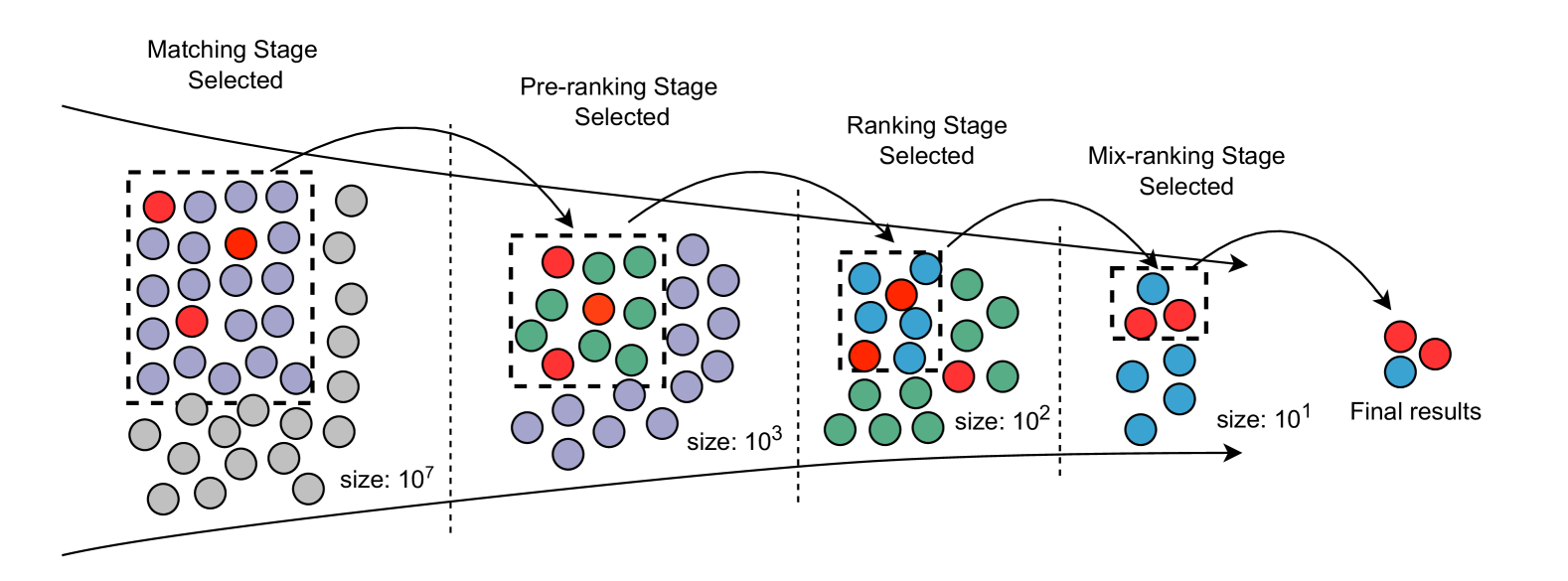
Figure 1: A typical cascade ranking architecture, including four stages: Matching, Pre-ranking, Ranking, and Mix-ranking. The red points represent the ground truth for the selection.

Early traditional training approaches for cascade ranking systems often optimize each stage in isolation, constructing samples, designing learning objectives, and defining proxy losses separately [5, 2, 12, 4, 27, 16, 24, 29]. This fragmented approach overlooks the interactions between stages, leading to suboptimal alignment with the overall system objective. Specifically, two key challenges arise: 1) Misalignment of Training Objectives: Cascade ranking aims to collaboratively select all relevant items from the ground truth set across multiple stages. However, each stage’s learning targets optimized by pointwise or pairwise losses are often more strict than the collaborative goal of cascade ranking. This misalignment may lead to inefficiency, particularly in recommendation scenarios where the model capacity is typically limited. 2) Lack of Learning to Collaborate: During online serving, different stages in a cascade ranking system will interact and collaborate with each other. Efficient interactions and collaborations are crucial for improving the overall performance of the cascade ranking system. For example, a Retrieval model can preemptively avoid items that the ranking model tends to overestimate, while the Ranking model can accurately identify ground-truth items from the recalled set. However, when models for different stages are trained independently, they lack the ability to learn these interactions and collaborations, which may lead to degraded testing performance.

Recent works have attempted to address these challenges. ICC [6] is an early study to address challenge 1) by fusing the predicted scores of different stages and optimizing them jointly through LambdaRank [3]. RankFlow [22] introduces an iterative training paradigm that dynamically determines the training samples for each stage by its upstream stage to address challenge 2). Although RankFlow reports significant improvements over both independent training and ICC, its iterative training process can lead to increased complexity and instability during training. FS-LTR [31] tackles challenge 2) by learning online patterns of interactions and collaborations with full-stage training samples and outperforms RankFlow. However, neither RankFlow nor FS-LTR explicitly addresses the misalignment of training objectives. ARF [28] emphasizes that learning targets should align with the objective of cascade ranking and proposes a new surrogate loss for Recall based on differentiable sorting. However, ARF focuses on a single stage and cannot fully address challenges 1) and 2). Additionally, ARF is prone to gradient vanishing when sorting many items, further limiting its applicability.

To the best of our knowledge, no existing approach simultaneously addresses both challenges, highlighting the need for a more comprehensive solution.

To address these challenges, we propose LCRON (Learning Cascade Ranking as One Network), introducing two types of novel surrogate losses. First, we propose a novel surrogate loss $L_{e2e}$, which is the lower bound of a differentiable approximation of the survival probability of ground-truth items through the entire cascade ranking system. $L_{e2e}$ directly aligns the learning objective with the global goal of the cascade ranking system, while naturally learning effective collaboration patterns for different stages. However, optimizing $L_{e2e}$ alone may lead to insufficient supervision for individual stages, especially when the survival probability at a particular stage is close to 0. In addition, we derive the lower bound and find that the tightness of the bound is highly related to the consistency of different stages. Therefore, we design a surrogate loss $L_{single}$ towards the Recall of each single stage, which enforces the model to distinguish ground-truth items from the entire candidate set rather than the filtered subset from upstream stages. $L_{single}$ can tighten the theoretical bound of $L_{e2e}$ and provides additional effective supervision when the survival probability of ground-truth items in $L_{e2e}$ is close to 0. Inspired by ARF [28], we use differentiable sorting techniques as the foundation of our surrogate losses. They inherit the main idea of the $L_{Relax}$ loss in ARF and avoid its gradient vanishing by a proper normalization. Finally, following ARF, we combine different losses ($L_{e2e}$ and each stage’s $L_{single}$ loss) in a UWL [11] form to reduce the number of hyperparameters, enhancing its practicality and robustness.

To verify the effectiveness of our method, we conduct extensive experiments on both public and industrial benchmarks. We conduct public experiments on RecFlow [15], the only public benchmark based on a real-world recommendation system that contains multi-stage samples of cascade ranking. The results on the public benchmark show that LCRON outperforms all baselines under the streaming evaluation (where for any day $t$ as a test, its training data comes from the beginning up to day $t-1$), indicating the effectiveness and robustness of our method. The ablation study highlights the role of different components of LCRON. The industrial experimental results show that LCRON consistently outperforms the best two baselines in public experiments on end-to-end Recall. We further conduct an online A/B experiment in a real-world advertising system. Compared to FS-LTR, LCRON brings about a 4.10% increase in advertising revenue and a 1.60% increase in the number of user conversions, demonstrating that our approach has significant commercial value for real-world cascade ranking systems.

2 Problem Formulation

We first introduce the formulation of a cascade ranking system. In such systems, a large initial set of candidate items is processed through a series of consecutive filtering stages to identify the most relevant or optimal results efficiently. Each stage applies a specific model $\mathcal{M}_{i}$ to evaluate and select a subset of items from the input set for the next stage. Let $T$ denote the total number of stages in the cascade, with an initial candidate inventory size of $q_{0}$. For any given stage $i$, we define the sample space of input candidates as $\mathcal{Q}_{i-1}$, which contains $q_{i-1}$ items. After processing by the $i$-th stage model, the output consists of $q_{i}$ selected items. Note that $q_{i}$ typically decreases as $i$ increases.

The models in the cascade ranking system are typically trained using specific paradigms, with training samples derived from the system itself. To rank the items, we define $\mathcal{F}^{\downarrow}_{\mathcal{M}}(\mathcal{S})$ as the ordered terms vector of set $\mathcal{S}$ sorted by the score of model $\mathcal{M}$ in descending order, and $\mathcal{F}^{\downarrow}_{\mathcal{M}}(\mathcal{S})[:K]$ as the top $K$ terms of $\mathcal{F}^{\downarrow}_{\mathcal{M}}(\mathcal{S})$. With the set of trained models $\{\mathcal{M}_{i}\mid 1\leq i\leq T\}$, the final output set $CS_{out}$ of the cascade ranking system can be obtained through a sequential filtering operation. This process can be formulated as:

$$CS_{out}=\mathcal{F}^{\downarrow}_{\mathcal{M}_{T}}((\cdots\mathcal{F}^{\downarrow}_{\mathcal{M}_{1}}(\mathcal{Q}_{0})[:q_{1}]\cdots))[:q_{T}]$$ (1)

We define the ground truth set $CS_{gt}$ as the set of items considered relevant or optimal based on user feedback or expert annotations. The goal of training paradigms for cascade ranking is to optimize the Recall of $CS_{gt}$ using training data collected from the system, which can be formulated as Eq 2, where $q_{T}$ is the size of $CS_{out}$, $\mathcal{K}$ is the size of $CS_{gt}$, and $\mathcal{K}<q_{T}$. Here, $\textbf{1}(\cdot)$ is the indicator function that returns 1 if the condition is true and 0 otherwise.

$$Recall@\mathcal{K}@q_{T}=\frac{\sum\limits_{i=1}^{q_{T}}\textbf{1}(item_{i}\in CS_{out})\textbf{1}(item_{i}\in CS_{gt})}{\sum\limits_{j=1}^{\mathcal{K}}\textbf{1}(item_{j}\in CS_{gt})}$$ (2)

Most previous works design training sets and methodologies for different stages separately, while a few attempt to build universal training paradigms, as detailed in Section 3. In this paper, we propose an all-in-one training paradigm for cascade ranking systems, which addresses the limitations of previous approaches and is detailed in Section 4.

3 Related Work

3.1 Learning Methodologies for Cascade Ranking

Cascade ranking [26, 13] is widely used in online recommendation and advertising systems to balance performance and resource efficiency. It employs multiple models with varying capacities to collaboratively select top-$k$ items from the entire inventory. Early traditional training approaches for cascade ranking systems often optimize each stage separately, with distinct training sample organization, learning objectives, and surrogate losses. There are three common learning tasks in cascade ranking systems: 1) probability distribution estimation (e.g., pCTR), which aims to optimize the accuracy of probability estimation and order and uses surrogate losses such as BCE, BPR, or their hybrid [32, 16, 24, 10]. The training samples include both positive and negative samples after exposure. 2) continuous value estimation (e.g., video playback time, advertising payment amount), which usually employs surrogate losses such as ordinal regression to optimize the model [17, 14]. It focuses on learning continuous values after specific user behaviors occur (e.g., viewing time after video exposure). 3) learning-to-rank, which is more commonly used in the retrieval stage of cascade ranking systems, with the entire or partial order of the ranking stage as the ground truth. It leverages methods such as pointwise, pairwise, and listwise approaches [5, 12, 27, 29, 4]. While these methods are widely adopted, they often fail to align training objectives with the global goal of cascade ranking and overlook the interactions between different stages.

Recently, several works have attempted to address these challenges by proposing interaction-aware training paradigms to jointly train the entire cascade ranking system. ICC [6] fuses the predictions of different stages and optimizes the fusion score using LambdaRank [3]. However, it suffers from the sample selection bias issue, where models are unaware of the sample spaces before exposure. RankFlow [22] introduces an iterative training paradigm. Each stage is trained with samples generated by its upstream stage and distills knowledge from its downstream model. While RankFlow reports significant improvements over ICC, its iterative training process may increase complexity and instability. FS-LTR [31] argues that each stage model should be trained with full-stage samples. It trains the cascade ranking system using full-stage samples and LambdaRank loss to learn the interaction and collaboration patterns of the online system, achieving better results than RankFlow. However, both FS-LTR and RankFlow fail to fully align with the global goal of cascade ranking. Another approach, ARF [28], emphasizes the importance of aligning learning targets with the Recall of cascade ranking and proposes surrogate losses based on differentiable sorting to optimize Recall. However, ARF focuses only on a single stage and assumes that downstream models are optimal, limiting its applicability. In this paper, we propose LCRON for end-to-end alignment with the global objective of cascade ranking, addressing the aforementioned challenges.

3.2 Differentiable Techniques for Hard Sorting

Differentiable sorting techniques provide continuous relaxations of the sorting operation, enabling end-to-end training within deep learning frameworks. Early work by Grover et al.(2019) introduced NeuralSort, which approximates hard sorting by generating a unimodal row-stochastic matrix. Subsequently, Prillo and Eisenschlos(2020) proposed SoftSort, a more lightweight and efficient approach for differentiable sorting. Recent advances, such as those in Petersen et al. [18, 19], Sander et al. [23], have further improved the performance and efficiency of differentiable sorting operators. These techniques have been widely adopted in various domains, including computer vision [7, 1, 23], online recommendation and advertising [25, 28, 20]. In this paper, we leverage differentiable sorting operators to construct surrogate losses for our task.

4 Methodology

In this section, we introduce our proposed method LCRON, which is the abbreviation of "Learnig Cascade Ranking as One Network". In Section 4.1, we give the organization of full-stage training samples, which mainly follows Zheng et al.(2024). In Section 4.2, we introduce a novel loss $L_{e2e}$ that directly optimizes the lower bound of a differentiable approximation of Equation 2, ensuring alignment with the overall objective of cascade ranking. In section 4.3, we discuss the limitations of $L_{CS}$ and introduce $L_{single}$ as auxiliary loss for each single stage to tight the theoretical bound of $L_{e2e}$ and provide additional effective supervision.

4.1 Full-Stage Training Samples of Cascade Ranking

For simplicity, we illustrate our method using a two-stage cascade ranking system ($T=2$), which can be readily extended to systems with additional stages. We downsample items from all stages of the cascade ranking system to construct full-stage training samples, primarily following FS-LTR [31].

Let $\mathcal{M}_{1}$ and $\mathcal{M}_{2}$ denote the retrieval and ranking models, respectively. The input space of $\mathcal{M}_{1}$, the input and output spaces of $\mathcal{M}_{2}$ are $\mathcal{Q}_{0}$, $\mathcal{Q}_{1}$, and $\mathcal{Q}_{2}$. We denote the ground-truth set as $CS_{gt}$, also referred to as $\mathcal{Q}_{3}$. For a given impression, let $u$ represent the user information and $item_{j}$ represent the item information. Let $y_{j}$ denote the label for the pair $(u,item_{j})$ and $\textbf{y}=(y_{1},y_{2},\dots,y_{N})$. The training samples for one impression can be formulated as Eq 3:

$$\begin{split}D&=\left(u,\{(item_{j},y_{j})\mid 0\leq j<N\}\right)\\ &=\left(u,\bigcup_{i=0}^{3}\{(item_{j},y_{j})\mid 0\leq j<n_{i}\text{ and }item_{j}\in\mathcal{Q}_{i}\}\right)\end{split}$$ (3)

where $n_{i}$ is the number of samples drawn from $\mathcal{Q}_{i}$ and $N=n_{0}+n_{1}+n_{2}+n_{3}$. In LCRON, the construction of full-stage training samples is a fundamental component of our approach. While specific sampling strategies and hyper-parameters (e.g., $n_{i}$) may influence the performance, their detailed analysis is beyond the scope of this paper. In both public and online experiments, all methods are evaluated on the same sampled datasets to ensure a fair comparison.

Let $R_{j}$ denote the descending rank index (where a higher value indicates a better rank) for the pair $(u,item_{j})$ within its sampled stage. The label $y_{j}$ is determined by both the stage order and the rank within the stage. Specifically, for any two pairs $(u,item_{i})$ and $(u,item_{j})$, the label $y_{i}$ and $y_{j}$ satisfy the following condition:

$$\textbf{1}(y_{i}>y_{j})=\textbf{1}(\mathcal{S}_{i}>\mathcal{S}_{j})\lor\left(\textbf{1}(\mathcal{S}_{i}=\mathcal{S}_{j})\land\textbf{1}(R_{i}>R_{j})\right)$$ (4)

where $\mathcal{S}_{i}>\mathcal{S}_{j}$ indicates that $item_{i}$ belongs to a later stage than $item_{j}$, and $R_{i}>R_{j}$ indicates that $item_{i}$ has a higher rank than $item_{j}$ within the same stage.

4.2 End-to-end Surrogate Loss for Top-K Cascade Ranking

Our goal is to design an efficient surrogate loss that aligns with the $Recall@\mathcal{K}@q_{2}$ metric of the entire cascade ranking system. We can transform the problem of optimizing the $Recall@\mathcal{K}@q_{2}$ of cascade ranking into a survival probability problem, allowing the model to estimate the probability that the ground truth is selected by the cascade ranking. Note that $\mathcal{K}$ is the size of $CS_{gt}$. Let $\mathcal{M}_{i}(D)\in\mathbb{R}^{1\times N}$ denote the prediction vector of $\mathcal{M}_{i}$ on the training data $D$. Let $P_{\mathcal{M}_{i}}^{q_{i}}$ represent the probability vector of each ad in $D$ being selected by the cascade ranking for top-$q_{i}$ selection. $q_{i}$ is the quota of $\mathcal{M}_{i}$, as mentioned in Section 2. The sum of $P_{\mathcal{M}_{i}}^{q_{i}}$ should be $q_{i}$. Let the survival probability vector output by the system be $P_{CS}^{q_{2}}$, and let the label y be a 0/1 vector indicating whether it is the ground truth. We can employ a log-loss of $P_{CS}^{q_{2}}$ and y to optimize the probability of the ground truth being selected by the cascade ranking as shown in Equation 5:

$$\begin{split}L(P_{CS}^{q_{2}},\textbf{y})&=-\sum_{i}(y_{i}\ln((P_{CS}^{q_{2}})_{i})\end{split}$$ (5)

Note that Eq 5 only uses items with $y=1$ (i.e., ground-truth items) to optimize $P_{CS}^{q_{2}}$ because we aim to ensure that the optimization objective is Recall, which focuses on whether the $K$ ground-truth items appear in the top $q_{2}$ set of predictions (typically $K<q_{2}$). It does not emphasize the quality of the other items in the top $q_{2}$ set. If items with $y=0$ are used as supervisory signals, the physical meaning of the optimization objective would shift towards binary classification.

Let $\pi\in\{0,1\}^{N}$ denote the sampling result from $P_{\mathcal{M}_{1}}^{q_{1}}$, and let $P_{\pi}$ represent the probability of sampling $\pi$. Then, $P_{\pi}$ can be formulated as Eq 6:

$$\begin{split}P_{\pi}=\frac{\prod_{i:\pi_{i}=1}(P_{\mathcal{M}_{1}}^{q_{1}})_{i}}{\sum_{S\subseteq[N],|S|=T}\prod_{j\in S}(P_{\mathcal{M}_{1}}^{q_{1}})_{j}}\end{split}$$ (6)

Then $P_{CS}^{q_{2}}$ can be expressed as Eq 7:

$$\begin{split}P_{CS}^{q_{2}}=\mathbb{E}_{\pi\sim P_{\pi}}\frac{(P_{\mathcal{M}_{2}}^{q_{2}}\odot\pi)}{\langle\pi,P_{\mathcal{M}_{2}}^{q_{2}}\rangle/\langle\textbf{1},P_{\mathcal{M}_{2}}^{q_{2}}\rangle}\end{split}$$ (7)

where $P_{\mathcal{M}_{2}}^{q_{2}}$ and $P^{q2}_{CS}$ are vectors. $\langle\cdot,\cdot\rangle$ denotes dot product, and $\odot$ denotes element-wise product. 1 represents a vector where all elements are 1. Due to the intractability of directly optimizing $P_{CS}^{q_{2}}$ caused by sampling and integration operations, we aim to find an approximate surrogate for $P_{CS}^{q_{2}}$. We define $\widehat{P_{CS}^{q_{2}}}=\prod_{i}^{2}P_{\mathcal{M}_{i}^{q_{i}}}$. It can be shown that $\widehat{P_{CS}^{q_{2}}}$ serves as an lower bound for $P_{CS}^{q_{2}}$, as demonstrated in Eq. 8, since $0\leq\langle\pi,P_{\mathcal{M}_{2}}^{q_{2}}\rangle/\langle\textbf{1},P_{\mathcal{M}_{2}}^{q_{2}}\rangle\leq 1$ always holds:

$$\begin{split}P_{CS}^{q_{2}}&=\mathbb{E}_{\pi\sim P_{\pi}}\frac{P_{\mathcal{M}_{2}}^{q_{2}}\odot\pi}{\langle\pi,P_{\mathcal{M}_{2}}^{q_{2}}\rangle/\langle\textbf{1},P_{\mathcal{M}_{2}}^{q_{2}}\rangle}\\ &\geq\mathbb{E}_{\pi\sim P_{\pi}}P_{\mathcal{M}_{2}}^{q_{2}}\odot\pi\\ &=\prod_{i}^{2}P_{\mathcal{M}_{i}}^{q_{i}}\\ &=\widehat{P_{CS}^{q_{2}}}.\end{split}$$ (8)

The next question is how to obtain a differentiable $P_{\mathcal{M}_{i}}^{q_{i}}$, enabling us to optimize $\widehat{P_{CS}^{q_{2}}}$. To achieve this, we introduce the permutation matrix as the foundation of our approach. For a given vector $x$ and its sorted counterpart $y$, there exists a unique permutation matrix $\mathcal{P}$ such that $y=\mathcal{P}x$. The elements of $\mathcal{P}$ are binary, taking values of either 0 or 1. Let $\mathcal{P}^{\downarrow}_{(\cdot)}$ denote the permutation matrix that sorts the vector $(\cdot)$ in descending order. Specifically, $(\mathcal{P}^{\downarrow}_{x})_{i,j}=1$ indicates that $x_{j}$ is the $i$-th largest element in $x$.

Using the permutation matrix, the top-$k$ elements of $D$ selected by $\mathcal{M}_{i}$ can be formulated as:

$$\mathcal{M}_{i}^{\downarrow}(k)=\sum^{k}_{j=1}(\mathcal{P}^{\downarrow}_{\mathcal{M}})_{j,:}$$ (9)

where $\mathcal{M}^{\downarrow}(k)\in\mathbb{R}^{1\times n}$ is a binary vector indicating whether each item is selected by the model, and $(\mathcal{P}^{\downarrow}_{\mathcal{M}})_{j,:}$ represents the $j$-th row of the permutation matrix for model $\mathcal{M}$.

It is evident that $P_{\mathcal{M}_{i}}^{q_{i}}$ can be interpreted as the distribution of $\mathcal{M}_{i}^{\downarrow}(q_{i})$, where $\mathcal{M}_{i}^{\downarrow}(q_{i})$ denotes the deterministic top-$q_{i}$ selection obtained through hard sorting (represented as a binary posterior observation, i.e., 1/0). To enable gradient-based optimization, we can relax $\mathcal{M}_{i}^{\downarrow}(q_{i})$ into the stochastic $P_{\mathcal{M}_{i}}^{q_{i}}$ and optimize it via maximum likelihood. Specifically, this can be achieved by relaxing the hard permutation matrix $\mathcal{P}$ (which sorts items in descending order) into a soft permutation matrix $\hat{\mathcal{P}}$ via differentiable sorting techniques [7, 21, 18]. Differentiable sorting methods typically generate $\hat{\mathcal{P}}$ as a row-stochastic matrix (each row sums to 1) by applying row-wise softmax with a temperature parameter $\tau$. As $\tau\to 0$, $\hat{\mathcal{P}}$ converges to the hard permutation matrix $\mathcal{P}$.

Let $\hat{\mathcal{P}}^{\downarrow}_{\mathcal{M}_{i}}\in[0,1]^{N\times N}$ be the soft permutation matrix for model $\mathcal{M}_{i}$, where $(\hat{\mathcal{P}}^{\downarrow}_{\mathcal{M}_{i}})_{j,k}$ represents the soft probability that item $k$ is ranked at position $j$. Then, we can formulate the top-$q_{i}$ selection probability $P_{\mathcal{M}_{i}}^{q_{i}}$ and the end-to-end loss $L_{e2e}$ of the cascade ranking system as Eq 10 and Eq 11:

$$\begin{split}P_{\mathcal{M}_{i}}^{q_{i}}&=\frac{\sum_{j=1}^{q_{i}}(\hat{\mathcal{P}}^{\downarrow}_{\mathcal{M}_{i}})_{j,:}}{\oslash~sp(\sum_{t=1}(\hat{\mathcal{P}}^{\downarrow}_{\mathcal{M}_{i}})_{t,:})}\end{split}$$ (10)

$$\begin{split}L_{e2e}&=-\sum_{j}y_{j}ln(\prod^{2}_{i}\frac{\sum_{j=1}^{q_{i}}(\hat{\mathcal{P}}^{\downarrow}_{\mathcal{M}_{i}})_{j,:}}{\oslash~sp(\sum_{t=1}(\hat{\mathcal{P}}^{\downarrow}_{\mathcal{M}_{i}})_{t,:})}\end{split}$$ (11)

where $\frac{\cdot}{\oslash\cdot}$ represents the element-wise division operator. In Eq 10, we perform an element-wise division to ensure that the probability values are normalized, as some differentiable sorting operators cannot guarantee column-wise normalization, such as NeuralSort [7] and SoftSort [21]. “$sp$” denotes that a stop gradient is needed during training. The end-to-end loss $L_{e2e}$ in Eq. 11 directly optimizes the joint survival probability through all cascade stages.

Traditional losses often impose strict constraints, which become problematic when model capacity is insufficient to satisfy all constraints. In contrast, $L_{e2e}$ directly aligns the learning objective of the goal of cascade ranking, allowing models to prioritize critical rankings while tolerating minor errors in less important comparisons. In addition, when a stage assigns a low score to a ground-truth item, $L_{e2e}$ not only optimizes that particular stage but also encourages other stages to improve their scores for the same ground-truth item. This adaptive mechanism enables an efficient collaborative pattern to be learned across stages, enhancing the overall survival probability of ground-truth items in the cascade ranking system.

4.3 Auxillary Loss of Single Stage and the Total Loss

Although $L_{e2e}$ directly optimizes the joint survival probability of ground-truth items through the entire cascade ranking system, it may suffer from two weaknesses: 1) $L_{e2e}$ is derived as a lower bound of the joint survival probability (see Section 4.2), the tightness of this bound could influence the overall performance, but $L_{e2e}$ can not optimize this bound itself, 2) it may suffer from insufficient supervision when the survival probability at a particular stage is close to 0. This issue is particularly pronounced during the initial training phase, where if all stages assign low scores to ground-truth items, the gradients across all models will also be small. This case makes it difficult to successfully warm up the models, leading to slow or ineffective learning.

According to Eq 8, the bound depends on the magnitude of $\frac{q_{2}}{\langle\pi,P^{q2}_{\mathcal{M}_{2}}\rangle}$, and the equation holds as $\frac{q_{2}}{\langle\pi,P^{q2}_{\mathcal{M}_{2}}\rangle}$ approaches 1. Since $\pi\sim P_{\pi}$, it is evident that optimizing the difference between $\mathcal{M}_{1}(D)$ and $\mathcal{M}_{2}(D)$ can help tighten the bound. We provide detailed analysis in appendix A.

To address these issues, we propose $L_{single}^{\mathcal{M}_{i}}$ for each single model, which is shown in Eq 12. $L_{single}$ provides the same supervision for both retrieval and ranking models, thereby optimizing the consistency of $\mathcal{M}_{1}(D)$ and $\mathcal{M}_{2}(D)$ and leading to a tight bound of $L_{e2e}$. $L_{single}^{\mathcal{M}_{i}}$ forces each model to distinguish ground-truth items from the entire inventory, offering effective yet not overly strict additional supervision for each model. This helps address the insufficient supervision situation that may occur in the $L_{e2e}$ loss during the initial training phase. Furthermore, unlike $L_{Relax}$ in ARF, which uses a fixed normalization factor $\mathcal{K}$ (corresponding to the denominator in Eq 12), $L_{single}$ employs a more reasonable probability normalization scheme to avoid gradient vanishing issues when sorting large-scale candidate sets.

$$\begin{split}L_{single}^{\mathcal{M}_{i}}&=-\sum_{j}y_{j}ln(\frac{\sum_{j=1}^{\mathcal{K}}(\hat{\mathcal{P}}^{\downarrow}_{\mathcal{M}_{i}})_{j,:}}{\oslash~sp(\sum_{t=1}(\hat{\mathcal{P}}^{\downarrow}_{\mathcal{M}_{i}})_{t,:})}\end{split}$$ (12)

Inspired by ARF [28], we simply employ UWL [11] to balance the $L_{e2e}$ and $L_{single}$ to reduce the number of hyper-parameters. For the two-stage cascade ranking, the final loss is formulated as Eq 13, where $\alpha$, $\beta$ and $\gamma$ are trainable scalars.

$$\begin{split}L=\frac{L_{e2e}}{2\alpha^{2}}+\frac{L_{single}^{\mathcal{M}_{1}}}{2\beta^{2}}+\frac{L_{single}^{\mathcal{M}_{2}}}{2\gamma^{2}}+log_{2}(\alpha\beta\gamma)\end{split}$$ (13)

5 Experiments

5.1 Experiment Setup

We conduct comprehensive experiments on both public and industrial datasets. We conduct public experiments to verify the effectiveness of our proposed method and perform ablation studies along with in-depth analysis. We conduct online experiments to study the impact of our method on real-world cascade ranking applications. Here we mainly describe the setup for public experiments, and details of online experiments are described in section 5.5.

• Public Benchmark. We conduct public experiments based on RecFlow [15], which, to the best of our knowledge, is the only public benchmark that collects data from all stages of real-world cascade ranking systems. RecFlow includes data from two periods (denoted as Period 1 and Period 2), spanning 22 days and 14 days, respectively. While Period 2 is primarily designed for studying the distribution shift problem in recommendation systems, which is beyond the scope of this paper, we focus on Period 1 data as our testbed. To train the cascade ranking, we adopt four stages of samples: $rank\_pos$, $rank\_neg$, $coarse\_neg$ and $prerank\_neg$. Table 1 summarizes the dataset statistics.

  Table 1: Dataset Statistics of Public Benchmark.

  Stage	Users	Impressions	Items per impression	the range of labels
  rank_pos	38,193	6,062,348	10	[1,20]
  rank_neg	38,193	6,062,348	10	[21,21]
  coarse_neg	38,193	6,062,348	10	[22,22]
  prerank_neg	38,193	6,062,348	10	[23,23]

• Cascade Ranking Setup. We employ a typical two-stage cascade ranking system as the testbed, utilizing DIN [32] for the ranking model and DSSM [9] for the retrieval model. The retrieval and ranking models are completely parameter-isolated, ensuring no parameters are shared between stages. This design eliminates potential confounding effects from parameter sharing, enabling a fair comparison between different methods. In this setup, the retrieval model selects the top 30 items, and subsequently, the ranking model chooses the top 20 items out of these 30 for “exposure”. Each impression contains 10 ground-truth items, referred to $rank\_pos$, which serve as the ground truth for exposure evaluation. This setup aligns with the data structure of the benchmark, ensuring evaluation consistency with real-world cascade ranking scenarios.

• Evaluation. We employ $Recall@k@m$ defined in Equation 2 as the golden metric to evaluate the overall performance of the cascade ranking system. Corresponding to the cascade ranking and public benchmark setup, the $m$ and $k$ for the evaluation are $20$ and $10$, respectively. In order to explore the impact of different baselines on model learning at different stages, we also evaluate the $Recall@k@m$ and $NDCG@k$ of each model as auxiliary observation metrics for analysis.

  Following the mainstream setup for evaluating recommendation datasets, we use the last day of Period 1 as the test set to report the main results of our experiments (Section 5.3), while the second-to-last day serves as the validation set for tuning the hyperparameters of different methods, including the temperature parameters of ICC, ARF, and LCRON. Considering that industrial scenarios commonly employ streaming training, we further evaluate the performance of different methods by treating each day as a separate test set (in Section 5.4). In this setting, when day $t$ is designated as the test set, the corresponding training data encompass all days from the beginning of Period 1 up to day $t-1$.

• LCRON Setup. We employ NeuralSort [7] as the differentiable sorting operator, aligning with the baseline method ARF to ensure a fair comparison. We tune the sole hyper-parameter $\tau$ on the validation set, which controls the temperature of NeuralSort.

• Implementation Details. We utilize the training pipeline and implementations of DSSM and DIN models provided by the open-source code  from [15], and we primarily focus on implementing the training loss functions of baselines and our method. The Multi-layer Perceptron (MLP) of the user and item towers in DSSM are set to be [128, 64, 32]. The architecture of DIN’s MLP is [128, 128, 32, 1]. All offline experiments are implemented using PyTorch 1.13 in Python 3.7. We employ the Adam optimizer with a learning rate of 0.01 for training all methods. Following the common practice in online recommendation systems [15, 30], each method is trained for only one epoch. The batch size is set to 1024.

5.2 Competing Methods

We compare our method with the following state-of-the-art methods in previous studies.

• Binary Cross-Entropy (BCE). We treat the ’rank_pos’ samples as positive and others as negative to train a BCE loss. The retrieval model is trained with all stages samples in Table 1. The ranking model is trained with only rank_pos and rank_neg samples, following the classic setting of cascade ranking systems. The rank_pos is regarded as positive samples, and others are regarded as negative samples. It is denoted as "BCE" in the following.

• ICC. It’s an early study for joint learning the models of cascade ranking  [6], which fuse multi-stage predictions and optimize them by LambdaRank [3].

• RankFlow. Qin et al.(2022) propose RankFlow, a method that iteratively updates the retrieval and ranking models, achieving better results than ICC [6]. The training sample space for the ranking model is determined by the retrieval model, and the ranking model’s predictions are distilled back to the retrieval model.

• FS-LTR. Zheng et al.(2024) propose a method to train all models in a cascade ranking system using full-stage training samples and learning-to-rank surrogate losses, achieving better results than RankFlow [22]. Since Zheng et al.(2024) primarily focuses on the organization of training samples rather than the design of surrogate losses, we design two representative variants to cover a wide spectrum of LTR losses. The first variant, FS-RankNet, utilizes the RankNet [2] loss, a classic pairwise LTR method. The second variant, FS-LambdaLoss, utilizes the LambdaLoss [27] loss, an advanced listwise LTR method. These variants represent two fundamental paradigms in LTR, ensuring a comprehensive comparison.

• ARF. It is designed to adapt to varying model capacities and data complexities by introducing an adaptive target that combines “relaxed” loss and “global” loss [28]. We use ARF loss to train both the retrieval and ranking models. To further improve ARF, we introduce ARF-v2 as an enhanced baseline, which replaces the relaxed loss of ARF with our proposed $L_{single}$ (Section 4.3). We set the hyper-parameters corresponding to the $q$ of the cascade ranking system. For the retrieval model, we set the parameters $m$ and $k$ to 30 and 10, respectively. For the ranking model, we set these parameters to 20 for $m$ and 10 for $k$.

5.3 Main Results

Table 2 presents the main results of the public experiments conducted on RecFlow. LCRON significantly outperforms all baselines on the end-to-end (joint) Recall, demonstrating its effectiveness in optimizing cascade ranking systems. Notably, while LCRON does not dominate all individual stage metrics (e.g., the Recall of the Ranking model), it achieves substantial improvements in joint metrics, highlighting the importance of stage collaboration. This aligns with our design philosophy: LCRON fully considers the interaction and collaboration between different stages, enabling significant gains in joint performance even with modest improvements in single-stage metrics.

The results also reveal interesting insights about the baselines: 1) While FS-LambdaLoss shows strong performance, FS-RankNet performs poorly under the same sample organization. This indicates that the choice of learning-to-rank methods plays a critical role in optimizing cascade ranking systems. 2) ARF-v2 outperforms ARF in all metrics, validating that $L_{single}$ effectively mitigates gradient vanishing, as discussed in Section 4.3.

Table 2: Main results of Public experimental on RecFlow. $*$ indicates the best results. The number in bold means that our method outperforms all the baselines on the corresponding metric. Note that the $Recall@10@20$ of $Joint$ is the golden metric for the whole cascade ranking system. The test set is the last day, with the remaining data used for training.

Method/Metric	Joint	Ranking		Retrieval
Recall@10@20 $\uparrow$	Recall@10@20 $\uparrow$	NDCG@10 $\uparrow$	Recall@10@30 $\uparrow$	NDCG@10 $\uparrow$
BCE	0.8541	0.7041	0.8411	0.7158	0.9709∗
ICC	0.8137	0.6985	0.8104	0.6160	0.9292
RankFlow	0.8656	0.7277	0.8636	0.7086	0.9660
FS-RankNet	0.7886	0.6868	0.7911	0.6715	0.9326
FS-LambdaLoss	0.8674	0.7333∗	0.8668	0.7215∗	0.9689
ARF	0.8613	0.6629	0.8623	0.5547	0.9625
ARF-v2	0.8671	0.7267	0.8672	0.7123	0.9683
LCRON (ours)	0.8732∗	0.7291	0.8729∗	0.7151	0.9700

5.4 In-depth Analysis

We first conduct an ablation study to evaluate the contribution of each component in LCRON. Specifically, we analyze the impact of $L_{e2e}$ and $L_{single}$ by removing them individually. The results are summarized in Table 3. The ablation study demonstrates that both $L_{e2e}$ and $L_{single}$ are essential components of LCRON. While their removal may not lead to statistically significant changes in all the individual ranking or retrieval metrics, the joint evaluation metric consistently shows a statistically significant improvement. This suggests that the interaction effects between the two stages of the cascade ranking system are optimized more effectively with the collaboration of $L_{e2e}$ and $L_{single}$, enhancing the overall performance.

Table 3: Ablation study of LCRON. $*$ indicates the best results. Given that the absolute values of ablation results are quite close, each experiment was run 5 times, and the results are reported as $mean\pm std$. Bold numbers indicate that LCRON shows statistically significant improvements over each ablation model, as determined by a t-test at the 5% significance level. The test set is the last day, with the remaining data used for training.

Method/Metric	Joint	Ranking		Retrieval
Recall@10@20 $\uparrow$	Recall@10@20 $\uparrow$	NDCG@10 $\uparrow$	Recall@10@30 $\uparrow$	NDCG@10 $\uparrow$
LCRON	0.8732 $\pm$ 0.0005 ∗	0.7291 $\pm$ 0.0008 ∗	0.8729 $\pm$ 0.0004 ∗	0.7151 $\pm$ 0.0009	0.9700 $\pm$ 0.0003 ∗
-$L_{e2e}$	0.8710 $\pm$ 0.0013	0.7280 $\pm$ 0.0007	0.8707 $\pm$ 0.0012	0.7153 $\pm$ 0.0009∗	0.9695 $\pm$ 0.0007
-$L_{single}$	0.8712 $\pm$ 0.0004	0.7286 $\pm$ 0.0007	0.8712 $\pm$ 0.0005	0.7142 $\pm$ 0.0013	0.9692 $\pm$ 0.0006

In Section˜5.3, we report the results tested on the last day of the dataset. Although this is a mainstream test setting for recommendation benchmarks [31, 28, 15], we argue that it may not fully reflect real-world industrial scenarios, where models are typically trained in an online, streaming manner. To provide a more comprehensive evaluation, we conduct additional experiments under a streaming training setup, where each day is treated as a separate test set. Specifically, when day $t$ is designated as the test set, the training data encompass all days from the beginning up to day $t-1$. The results, shown in Figure 2, reveal two key observations: 1) In the initial phase (first 10 days), LCRON exhibits rapid convergence, matching the performance of ARF-v2 and significantly outperforming other baselines. 2) In the later phase (last 12 days), LCRON not only surpasses all baselines but also demonstrates a widening performance gap over time, indicating its superior adaptability and robustness in long-term industrial applications. These findings underscore LCRON’s ability to achieve both fast convergence and sustained performance improvements, making it a practical and effective solution for real-world cascade ranking systems.

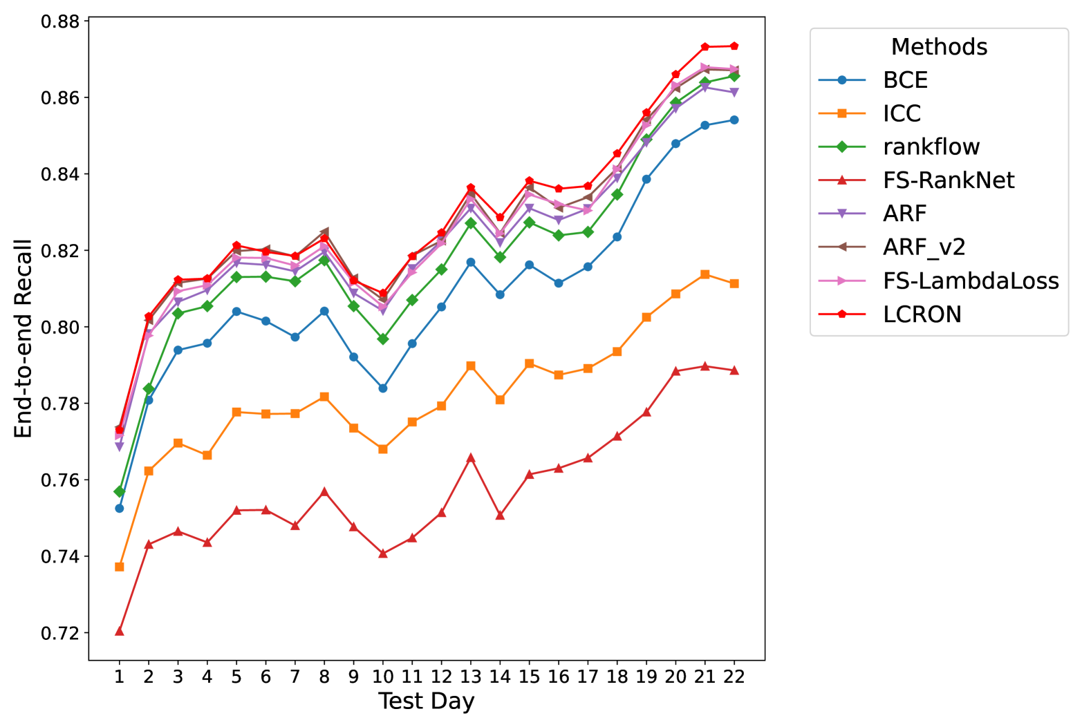
Figure 2: The evaluation results of different methods on RecFlow, in a streaming manner.

In addition, we investigate the impact of manually tuning the weights of $L_{e2e}$ and $L_{single}$ in LCRON. While the UWL formulation is designed to reduce hyperparameter tuning costs, it does not guarantee optimal performance theoretically. Table 4 shows the results of fixing $L_{e2e}$ to 1 and varying the weight of $L_{single}$. We observe that different weight configurations yield varying performance, with most configurations outperforming the baselines. The best manual configuration achieves a joint $Recall@10@20$ of 0.8733, which is almost the same as UWL-based LCRON. This suggests that while manual tuning can yield competitive results, UWL provides a robust and efficient way to combine $L_{e2e}$ and $L_{single}$ without extensive hyperparameter search.

Table 4: Experimental results of LCRON under fixed-weight configurations of $L_{e2e}$ and $L_{single}$. We fix $L_{e2e}$ to 1 and evaluate different weights for $L_{single}$. The test set is the last day, with the remaining data used for training.

weight of $L_{single}$	Joint	Ranking		Retrieval
Recall@10@20 $\uparrow$	Recall@10@20 $\uparrow$	NDCG@10 $\uparrow$	Recall@10@30 $\uparrow$	NDCG@10 $\uparrow$
0.01	0.8712	0.7294	0.8713	0.7122	0.9691
0.1	0.8706	0.7292	0.8706	0.7109	0.9686
0.5	0.8705	0.7279	0.8703	0.7132	0.9694
1	0.8723	0.7284	0.8723	0.7136	0.9691
2	0.8731	0.7295	0.8731	0.7132	0.9690
3	0.8730	0.7289	0.8730	0.7120	0.9694
4	0.8720	0.7293	0.8718	0.7118	0.9689
5	0.8733	0.7299	0.8730	0.7140	0.9697

Overall, these in-depth analyses, including the ablation study, streaming evaluation, and weight-tuning experiments, collectively demonstrate the robustness and practicality of LCRON in real-world cascade ranking systems. The ablation study confirms the necessity of both $L_{e2e}$ and $L_{single}$ for optimizing the interaction effects between ranking and retrieval stages. The streaming evaluation results further validate LCRON’s ability to adapt to dynamic, real-world scenarios, while the weight tuning experiments highlight the efficiency of the UWL formulation in reducing hyperparameter tuning efforts without sacrificing performance. These findings solidify LCRON as a strong candidate for industrial applications, offering a balanced combination of performance, adaptability, and ease of deployment. We also supply a sensitivity analysis in appendix C.

5.5 Online Deployment

To study the impact of LCRON on real-world industrial applications, we further deploy LCRON on a large-scale advertising system. Due to the scarcity of online resources, we opted to select only the two best-performing baselines from the public experiment along with LCRON for the online A/B test. Each experimental group was allocated 10% of the online traffic. Each model was trained using an online learning approach and was deployed online after seven days of training, followed by a 15-day online A/B test. Due to the space limitation, implementation details are described in appendix B. The results of the online experiments, as shown in Table 5, demonstrate that our LCRON model achieves significant improvements in both revenue and ad conversions compared to the two baseline methods, FS-LambdaLoss and ARF-v2. Notably, LCRON delivers superior performance in both public and industrial experiments, where variations in data size and model architecture are present. This indicates not only the effectiveness but also the robust generalization capabilities of our approach.

Table 5: Industrial experimental results for 15 days on a real-world advertising system. Each method was allocated 10% of the online traffic. For online metrics, we calculate the relative improvement of other methods compared to FS-LambdaLoss as the baseline.

Method/Metric	Offline Metrics	Online Metrics
Joint Recall	Revenue	Ad Conversions
FS-LambdaLoss	0.8210	–	–
ARF-v2	0.8237	+1.66%	+0.65%
LCRON (ours)	0.8289	+4.1%	+1.6%

6 Conclusion

In this paper, we present a novel training framework for cascade ranking, incorporating two complementary loss functions: $L_{e2e}$ and $L_{single}$. $L_{e2e}$ optimizes a lower bound of the survival probability of ground-truth items throughout the cascade ranking, ensuring theoretical consistency with the system’s global objective (i.e., End-to-end Recall). To address the limitations of $L_{e2e}$, we introduce $L_{single}$, which tightens the bound and provides additional supervisory signals. We conduct extensive experiments on both public and industrial benchmarks, along with online A/B testing, demonstrating the effectiveness of our proposed LCRON framework and showing significant improvements in end-to-end Recall, revenue, and user conversion numbers. We believe this work can have a broad positive impact on various areas, such as recommendation systems, advertising, and search technologies.

Appendix A Theoretical Analysis for the Bound of $P_{CS}^{q_{2}}$ and $\widehat{P_{CS}^{q_{2}}}$

Here, we provide a more detailed analysis of the bound for $P_{CS}^{q_{2}}$ and $\widehat{P_{CS}^{q_{2}}}$, and explain why $L_{single}$ can tighten the bound.

The gap between $P_{CS}^{q_{2}}$ and $\widehat{P_{CS}^{q_{2}}}$ can be formulated as Eq. 14:

$$\begin{split}\Delta&=P_{CS}^{q_{2}}-\widehat{P_{CS}^{q_{2}}}\\ &=\mathbb{E}_{\pi\sim P_{\pi}}\left[\frac{P_{\mathcal{M}_{2}}^{q_{2}}\odot\pi}{\langle\pi,P_{\mathcal{M}_{2}}^{q_{2}}\rangle/q_{2}}-P_{\mathcal{M}_{2}}^{q_{2}}\odot\pi\right]\\ &=\mathbb{E}_{\pi\sim P_{\pi}}\left[P_{\mathcal{M}_{2}}^{q_{2}}\odot\pi\left(\frac{q_{2}}{\langle\pi,P_{\mathcal{M}_{2}}^{q_{2}}\rangle}-1\right)\right]\\ &\leq\mathbb{E}_{\pi\sim P_{\pi}}\left[P_{\mathcal{M}_{2}}^{q_{2}}\left(\frac{q_{2}}{\langle\pi,P_{\mathcal{M}_{2}}^{q_{2}}\rangle}-1\right)\right]\\ &=\left[P_{\mathcal{M}_{2}}^{q_{2}}\left(\frac{q_{2}}{\mathbb{E}_{\pi\sim P_{\pi}}\langle\pi,P_{\mathcal{M}_{2}}^{q_{2}}\rangle}-1\right)\right]\\ &=\left[P_{\mathcal{M}_{2}}^{q_{2}}\left(\frac{q_{2}}{\langle P_{\mathcal{M}_{1}}^{q_{1}},P_{\mathcal{M}_{2}}^{q_{2}}\rangle}-1\right)\right]\\ &=\Delta^{{}^{\prime}}\end{split}$$ (14)

Here, we have derived a theoretical upper bound for $\Delta$, denoted as $\Delta^{{}^{\prime}}$. Note that $P^{q_{2}}_{\mathcal{M}_{2}}\in[0,1]^{N}$, $P^{q_{1}}_{\mathcal{M}_{1}}\in[0,1]^{N}$, and $\sum P^{q_{2}}_{\mathcal{M}_{2}}=q_{2}$, $\sum P^{q_{1}}_{\mathcal{M}_{1}}=q_{1}$.

Next, we consider how the relationship between the model outputs might affect $\Delta^{{}^{\prime}}$. For a given $P_{\mathcal{M}_{2}}^{q_{2}}$, treating $P_{\mathcal{M}_{2}}^{q_{2}}$ as the only variable to minimize $\Delta^{{}^{\prime}}$, it is evident that the following condition must be satisfied:

$$(P_{\mathcal{M}_{1}}^{q_{1}})_{i}=\begin{cases}1&\text{if }i\in\underset{i}{\operatorname{argTopK}}(P_{\mathcal{M}_{2}}^{q_{2}})\text{\quad(K=$q_{1}$)}\\ 0&\text{otherwise}\end{cases}$$ (15)

where $(P_{\mathcal{M}_{1}}^{q_{1}})_{i}$ represents the $i$-th element of the vector $P_{\mathcal{M}_{1}}^{q_{1}}$, and $\underset{i}{\operatorname{argTopK}}(P_{\mathcal{M}_{2}}^{q_{2}})$ denotes the indices of the top $K$ elements of $P_{\mathcal{M}_{2}}^{q_{2}}$. This indicates that if the top $q_{2}$ sets of the two models are consistent, it helps to reduce $\Delta^{{}^{\prime}}$. Of course, optimizing the consistency of the entire output distributions across different models also achieves the same goal, as this is a stronger constraint. Furthermore, if $(P_{\mathcal{M}_{1}}^{q_{2}})_{i}$ is a binary vector (i.e., its elements are either 0 or 1), then $\Delta$ achieves its minimum value ($\Delta^{{}^{\prime}}=0$) when Eq. 15 is satisfied.

The single-stage loss $L_{single}^{\mathcal{M}_{i}}$ (Eq. 12) directly optimizes the ranking consistency of each model with the same supervision (ground-truth labels), thereby implicitly aligning $\mathcal{M}_{1}(D)$ and $\mathcal{M}_{2}(D)$. This helps to reduce $\Delta^{{}^{\prime}}$, indirectly optimizing the bound $\Delta$. It is worth noting that there are many methods to optimize the consistency of model outputs, such as model distillation or minimizing the KL divergence between outputs. The $L_{single}$ we designed not only optimizes the consistency of output distributions across different models but also mitigates potential gradient vanishing issues in $L_{e2e}$ under certain circumstances, providing additional effective supervision signals.

Appendix B Implementation Details of Online Experiments

In this section, we provide additional details on the implementation of the online experiments. Our online system consists of four stages: Matching, Pre-ranking, Ranking, and Mix-ranking. However, for the purpose of this study, we focus on a two-stage cascade ranking setup, comprising the Matching (Retrieval) and Pre-ranking stages (illustrated in Figure 1). This design choice is motivated by several practical and methodological considerations: 1) Generality of Two-Stage Setup: The two-stage cascade ranking setup (Matching and Pre-ranking) does not lose generality, as it captures the core challenges of cascade ranking optimization, which are fundamental to any multi-stage ranking system. The insights gained from this setup can be extended to systems with more stages. 2) Practical Constraints: Conducting experiments on the entire four-stage system would introduce significant engineering challenges, particularly in data construction and model deployment. For instance, aligning the format of training logs and deployment details across all stages is non-trivial. Deploying and evaluating a full four-stage cascade ranking system in an online environment would require substantial infrastructure support, which is beyond the scope of this study.

Regarding the features, we utilize approximately 150 sparse features and 4 dense features. Sparse features are represented by embeddings derived from lookup tables, with each ID embedding having a dimensionality of 64. Dense features, on the other hand, directly use raw values or pre-trained model outputs, with a total dimensionality of 512. The Retrieval model includes all features used in the Pre-ranking model, except for combined features. Combined features refer to the process of integrating multiple individual features into a new, unified feature set to improve model performance. This technique captures interactions between different variables, providing richer information than each feature could individually. The combined features also fall under the category of sparse features. In our experiments, there are 20 combined features. In our experiments, models of different stages do not share any parameters.

Regarding the model architectures, we adopt DSSM for the retrieval stage and MLP for the Pre-ranking stage. For DSSM, the FFN layers’ size of both the user and item towers are [1024,256,256,64]. The layer size of the MLP is [1024,512,512,1]. We employ PRelu [8] as the activation function for hidden layers. We use HeInit [8] to initialize all the training parameters. We adopt batch normalization for each hidden layer and the normalization momentum is 0.999.

Regarding the training samples, we organize our training samples according to Section 4.1. We collect samples from the Matching, Pre-ranking, and Ranking stages, with items that succeed in the Ranking stage treated as ground-truth items. For each impression, we collect 20 items for training (i.e. $N=20$ in Section 4.1). The sample distribution across stages is defined by $n_{0}=5$, $n_{1}=5$, $n_{2}=8$ and $n_{3}=2$.

The models are trained in an online streaming manner. During each day of training, 20 billion (user, ad) pairs were processed. The optimizer is AdaGrad with a learning rate of 1e-2. All parameters are trained from scratch, without any pre-trained embeddings. The batch size is set to 4096 for both the retrieval and Pre-ranking models. Both the training and serving frameworks are developed based on TensorFlow. We use LCRON to train the retrieval and pre-rank model together and save unified checkpoints. Subsequently, by reconstructing two metadata files, these two models are deployed separately. During deployment, each model loads only the parameters corresponding to its own structure from the saved checkpoint during the joint training phase.

Appendix C Sensitivity Analysis on Hyper-parameters

We analyze the sensitivity of LCRON to its hyperparameter $\tau$, which controls the smoothness of the differentiable sorting operator. Table 6 summarizes the results for different values of $\tau$. The best performance is achieved at $\tau=50$. Even suboptimal values of $\tau$ within a wide range (e.g., $\tau=100$ or $\tau=200$) yield significant improvements over the baselines, demonstrating the robustness of LCRON to hyper-parameter choices. From the results, we observe that the performance seems to exhibit an unimodal trend with respect to $\tau$, peaking at $\tau=50$ and gradually decreasing as $\tau$ moves away from this value. This unimodal behavior provides practical guidance for hyperparameter tuning in real-world industrial applications, suggesting that a moderate value of $\tau$ is likely to yield near-optimal performance.

Table 6: Sensitivity analysis results of the hyper-parameter $\tau$ of LCRON on the public benchmark. The test set is the last day, with the remaining data used for training.

$\tau$	Joint	Ranking		Retrieval
Recall@10@20 $\uparrow$	Recall@10@20 $\uparrow$	NDCG@10 $\uparrow$	Recall@10@30 $\uparrow$	NDCG@10 $\uparrow$
1	0.8701	0.7276	0.8701	0.7071	0.9677
20	0.8709	0.7285	0.8708	0.7145	0.9696
50	0.8732	0.7291	0.8729	0.7151	0.9700
100	0.8722	0.7292	0.8719	0.7155	0.9707
200	0.8721	0.7278	0.8719	0.7156	0.9703
1000	0.8716	0.7285	0.8711	0.7197	0.9711

References

- Blondel et al. [2020] Mathieu Blondel, Olivier Teboul, Quentin Berthet, and Josip Djolonga. Fast differentiable sorting and ranking. In International Conference on Machine Learning, pages 950–959. PMLR, 2020.
- Burges et al. [2005] Christopher J. C. Burges, Tal Shaked, Erin Renshaw, Ari Lazier, Matt Deeds, Nicole Hamilton, and Gregory N. Hullender. Learning to rank using gradient descent. In ICML, pages 89–96, 2005.
- Burges [2010] Christopher JC Burges. From ranknet to lambdarank to lambdamart: An overview. Learning, page 81, 2010.
- Covington et al. [2016] Paul Covington, Jay Adams, and Emre Sargin. Deep neural networks for youtube recommendations. In Proceedings of the 10th ACM conference on recommender systems, pages 191–198, 2016.
- Crammer and Singer [2001] Koby Crammer and Yoram Singer. Pranking with ranking. In NeurIPS, pages 641–647, 2001.
- Gallagher et al. [2019] Luke Gallagher, Ruey-Cheng Chen, Roi Blanco, and J. Shane Culpepper. Joint optimization of cascade ranking models. In WSDM, pages 15–23, 2019.
- Grover et al. [2019] Aditya Grover, Eric Wang, Aaron Zweig, and Stefano Ermon. Stochastic optimization of sorting networks via continuous relaxations. In ICLR, 2019.
- He et al. [2015] Kaiming He, Xiangyu Zhang, Shaoqing Ren, and Jian Sun. Delving deep into rectifiers: Surpassing human-level performance on imagenet classification. In ICCV, pages 1026–1034, 2015.
- Huang et al. [2013] Po-Sen Huang, Xiaodong He, Jianfeng Gao, Li Deng, Alex Acero, and Larry Heck. Learning deep structured semantic models for web search using clickthrough data. In Proceedings of the 22nd ACM international conference on Information & Knowledge Management, pages 2333–2338, 2013.
- Huang et al. [2022] Siguang Huang, Yunli Wang, Lili Mou, Huayue Zhang, Han Zhu, Chuan Yu, and Bo Zheng. MBCT: tree-based feature-aware binning for individual uncertainty calibration. In WWW, pages 2236–2246, 2022.
- Kendall et al. [2018] Alex Kendall, Yarin Gal, and Roberto Cipolla. Multi-task learning using uncertainty to weigh losses for scene geometry and semantics. In CVPR, pages 7482–7491, 2018.
- Li et al. [2007] Ping Li, Christopher J. C. Burges, and Qiang Wu. Mcrank: Learning to rank using multiple classification and gradient boosting. In NeurIPS, pages 897–904, 2007.
- Li et al. [2023] Zhen Li, Chongyang Tao, Jiazhan Feng, Tao Shen, Dongyan Zhao, Xiubo Geng, and Daxin Jiang. FAA: fine-grained attention alignment for cascade document ranking. In ACL, pages 1688–1700, 2023.
- Lin et al. [2023] Xiao Lin, Xiaokai Chen, Linfeng Song, Jingwei Liu, Biao Li, and Peng Jiang. Tree based progressive regression model for watch-time prediction in short-video recommendation. In Proceedings of the 29th ACM SIGKDD Conference on Knowledge Discovery and Data Mining, pages 4497–4506, 2023.
- Liu et al. [2024] Qi Liu, Kai Zheng, Rui Huang, Wuchao Li, Kuo Cai, Yuan Chai, Yanan Niu, Yiqun Hui, Bing Han, Na Mou, et al. Recflow: An industrial full flow recommendation dataset. arXiv preprint arXiv:2410.20868, 2024.
- Ma et al. [2018] Xiao Ma, Liqin Zhao, Guan Huang, Zhi Wang, Zelin Hu, Xiaoqiang Zhu, and Kun Gai. Entire space multi-task model: An effective approach for estimating post-click conversion rate. In The 41st International ACM SIGIR Conference on Research & Development in Information Retrieval, pages 1137–1140, 2018.
- Niu et al. [2016] Zhenxing Niu, Mo Zhou, Le Wang, Xinbo Gao, and Gang Hua. Ordinal regression with multiple output cnn for age estimation. In Proceedings of the IEEE conference on computer vision and pattern recognition, pages 4920–4928, 2016.
- Petersen et al. [2021] Felix Petersen, Christian Borgelt, Hilde Kuehne, and Oliver Deussen. Differentiable sorting networks for scalable sorting and ranking supervision. In ICML, pages 8546–8555, 2021.
- Petersen et al. [2022] Felix Petersen, Christian Borgelt, Hilde Kuehne, and Oliver Deussen. Monotonic differentiable sorting networks. In ICLR, 2022.
- Pobrotyn and Białobrzeski [2021] Przemysław Pobrotyn and Radosław Białobrzeski. Neuralndcg: Direct optimisation of a ranking metric via differentiable relaxation of sorting. arXiv preprint arXiv:2102.07831, 2021.
- Prillo and Eisenschlos [2020] Sebastian Prillo and Julian Eisenschlos. Softsort: A continuous relaxation for the argsort operator. In International Conference on Machine Learning, pages 7793–7802. PMLR, 2020.
- Qin et al. [2022] Jiarui Qin, Jiachen Zhu, Bo Chen, Zhirong Liu, Weiwen Liu, Ruiming Tang, Rui Zhang, Yong Yu, and Weinan Zhang. Rankflow: Joint optimization of multi-stage cascade ranking systems as flows. In SIGIR, pages 814–824, 2022.
- Sander et al. [2023] Michael Eli Sander, Joan Puigcerver, Josip Djolonga, Gabriel Peyré, and Mathieu Blondel. Fast, differentiable and sparse top-k: a convex analysis perspective. In International Conference on Machine Learning, pages 29919–29936. PMLR, 2023.
- Sheng et al. [2023] Xiang-Rong Sheng, Jingyue Gao, Yueyao Cheng, Siran Yang, Shuguang Han, Hongbo Deng, Yuning Jiang, Jian Xu, and Bo Zheng. Joint optimization of ranking and calibration with contextualized hybrid model. In Proceedings of the 29th ACM SIGKDD Conference on Knowledge Discovery and Data Mining, pages 4813–4822, 2023.
- Swezey et al. [2021] Robin M. E. Swezey, Aditya Grover, Bruno Charron, and Stefano Ermon. Pirank: Scalable learning to rank via differentiable sorting. In NeurIPS, pages 21644–21654, 2021.
- Wang et al. [2011] Lidan Wang, Jimmy Lin, and Donald Metzler. A cascade ranking model for efficient ranked retrieval. In SIGIR, pages 105–114, 2011.
- Wang et al. [2018] Xuanhui Wang, Cheng Li, Nadav Golbandi, Michael Bendersky, and Marc Najork. The lambdaloss framework for ranking metric optimization. In CIKM, pages 1313–1322, 2018.
- Wang et al. [2024] Yunli Wang, Zhiqiang Wang, Jian Yang, Shiyang Wen, Dongying Kong, Han Li, and Kun Gai. Adaptive neural ranking framework: Toward maximized business goal for cascade ranking systems. In WWW, pages 3798–3809. ACM, 2024.
- Wu et al. [2024] Jiancan Wu, Xiang Wang, Xingyu Gao, Jiawei Chen, Hongcheng Fu, and Tianyu Qiu. On the effectiveness of sampled softmax loss for item recommendation. ACM Transactions on Information Systems, 42(4):1–26, 2024.
- Zhang et al. [2022] Zhao-Yu Zhang, Xiang-Rong Sheng, Yujing Zhang, Biye Jiang, Shuguang Han, Hongbo Deng, and Bo Zheng. Towards understanding the overfitting phenomenon of deep click-through rate models. In Proceedings of the 31st ACM international conference on information & knowledge management, pages 2671–2680, 2022.
- Zheng et al. [2024] Kai Zheng, Haijun Zhao, Rui Huang, Beichuan Zhang, Na Mou, Yanan Niu, Yang Song, Hongning Wang, and Kun Gai. Full stage learning to rank: A unified framework for multi-stage systems. In Proceedings of the ACM on Web Conference 2024, pages 3621–3631, 2024.
- Zhou et al. [2018] Guorui Zhou, Xiaoqiang Zhu, Chenru Song, Ying Fan, Han Zhu, Xiao Ma, Yanghui Yan, Junqi Jin, Han Li, and Kun Gai. Deep interest network for click-through rate prediction. In Proceedings of the 24th ACM SIGKDD international conference on knowledge discovery & data mining, pages 1059–1068, 2018.