Sequential Quadratic Optimization for Solving Expectation Equality Constrained Stochastic Optimization Problems

Abstract

A sequential quadratic programming method is designed for solving general smooth nonlinear stochastic optimization problems subject to expectation equality constraints. We consider the setting where the objective and constraint function values, as well as their derivatives, are not directly available. The algorithm applies an adaptive step size policy and only relies on objective gradient estimates, constraint function estimates, and constraint derivative estimates to update iterates. Both asymptotic and non-asymptotic convergence properties of the algorithm are analyzed. Under reasonable assumptions, the algorithm generates a sequence of iterates whose first-order stationary measure diminishes in expectation. In addition, we identify the iteration and sample complexity for obtaining a first-order $\varepsilon$-stationary iterate in expectation. The results of numerical experiments demonstrate the efficiency and efficacy of our proposed algorithm compared to a penalty method and an augmented Lagrangian method.

1 Introduction

In this paper, we design, analyze, and implement a sequential quadratic programming (SQP) method for minimizing a general smooth nonlinear function, which is written in an expectation format, subject to expectation equality constraints. Such optimization problems arise in various science and engineering applications, including but not limited to machine learning fairness [47], dynamic systems [56], PDE-constrained optimization [32], structural model estimation [57], and training physics-informed neural networks [2].

Numerous algorithms have been designed and analyzed for solving general nonlinear constrained deterministic optimization problems, including penalty methods, interior-point methods and SQP methods. The fundamental idea of penalty methods [16, 31, 61] is to incorporate constraint violations into the objective function using a weighted penalty term and then apply unconstrained optimization algorithms, such as subgradient methods [38, 55], to solve the resulting penalty subproblem. Penalty methods are easy to implement, however, they usually have inferior numerical performance compared to interior-point methods and SQP methods due to the difficulty in selecting suitable penalty parameters and the ill-conditioning of penalty subproblems. Meanwhile, interior-point methods [26, 54, 60] apply barrier functions to guide iterates moving along a central path within the feasible set to a solution. Interior-point methods are well-known for their outstanding numerical behaviors as they serve as base algorithms for many advanced computational optimization softwares, including IPOPT [58] and KNITRO [13]. Finally, SQP methods [10, 59] are another class of optimization algorithms that have superior performance in both theory and practice. Line-search SQP methods [35, 36, 51] are widely recognized as a class of state-of-the-art algorithms for solving equality-constrained optimization problems. At every iteration, SQP methods construct and solve a subproblem model of quadratic objective function subject to linearized constraints. This helps SQP methods allow infeasible iterates while (under reasonable conditions) enjoy global and fast local convergence behaviors at the same time.

To handle optimization problems arising in areas of machine learning and data science, it becomes crucial to design advanced algorithms for solving stochastic optimization problems subject to nonlinear constraints. When solving stochastic optimization problems with deterministic constraints, most of existing algorithms are either stochastic penalty methods (with relatively inferior numerical performance) or imposing strong conditions (e.g., convexity and boundedness) on the feasible set so that projection-type operations or linear-type operators (such as Frank-Wolfe methods) are tractable [15, 37, 40, 46, 53]. Recently, a few papers proposed novel algorithms such as stochastic interior-point methods and stochastic SQP methods. In particular, [21, 25] develop stochastic interior-point methods for solving stochastic (or noisy) optimization problems with deterministic box constraints, while [18, 20] extend the problem setting to general deterministic (potentially noisy) nonlinear constraints. Compared to stochastic interior-point methods, stochastic SQP methods have been studied more extensively in the literature. [6] proposed the very first stochastic SQP algorithm for solving deterministic nonlinear equality constrained stochastic optimization problems, while [44] is the first work that considers general deterministic functional constrained setting. There are multiple follow-up works based on [6, 44], including showing almost-sure convergence and non-asymptotic convergence properties of stochastic SQP algorithms [19, 22]; designing and analyzing stochastic line-search SQP methods [9, 43, 48, 52]; relaxing requirements of constraint qualifications [5, 8]; allowing inexactness when solving SQP subproblems [3, 4, 23, 45]; improving convergence behaviors via variance-reduced techniques [7]; designing stochastic trust-region SQP methods [29, 30]; and solving general deterministic nonlinear constrained stochastic optimization problems with an objective-function-free stochastic SQP method [24].

On the other hand, there are much less literature discussing general expectation-constrained stochastic optimization algorithms. We note that some proximal-type algorithms are proposed in [11, 39], however, relatively restrictive assumptions (including convexity of functions and “strong feasibility” conditions; see [11, Assumption 3]) are required for proving theoretical convergence results. Meanwhile, [27, 42] consider the “black-box” optimization setting, where trust-region and direct-search methods are developed respectively. Recently, a momentum-based stochastic penalty method has been designed by [17]. To the best of our knowledge, [28] proposes the only existing stochastic SQP method for solving expectation-constrained stochastic optimization problems, however, such algorithm relies on a special Monte Carlo process that generates stochastic search directions as unbiased estimators of the corresponding true search direction, while our proposed algorithm does not require such a restrictive unbiasedness condition.

1.1 Contributions

Our paper makes three-fold major contributions, which are summarized as follows.

Algorithmistic Perspective.  We design a stochastic SQP method to solve general nonlinear equality-constrained optimization problems, where both objective and constraint functions are represented as expectations. Our algorithm framework shares the spirit of [12, Algorithm 4.1] and [6, Algorithm 3.1] that only a few stochastic estimates need to be evaluated at each iteration, while these stochastic estimates are not necessarily satisfying any probablistic accuracy conditions as [9, 43]. Moreover, our proposed algorithm takes adaptive step sizes and never requires objective function estimates.

Theoretical Perspective.  Although our algorithmic framework is inspired by [6], our theoretical analysis differs as we focus on the stochastic constrained setting. In [6], when solving deterministic equality-constrained stochastic optimization problems, under reasonable assumptions, the proposed algorithm always computes stochastic search directions behaving as unbiased estimators of “real” search directions, which would be computed via corresponding deterministic quantities. However, such nice properties no longer hold in our setting due to uncertainty within constraints, which results in a different analysis from [6, 24]. Because of loose conditions required for stochastic estimates, we only present convergence in expectation properties of our proposed algorithm. We demonstrate asymptotic and non-asymptotic convergence properties of our method, including both iteration and sample complexity results. In particular, our algorithm’s theoretical performance is comparable to the behaviors of stochastic gradient type algorithms for unconstrained optimization problems [12, 49].

Numerical Perspective.  We present the empirical performance of our proposed algorithm by comparing it to the stochastic momentum-based method proposed in [17] on a constrained binary classification problem with five different datasets from the LIBSVM collection [14]. We also test and show the results of numerical experiments of our algorithm in contrast to a stochastic subgradient method on problems from the CUTEst collection [34]. These numerical comparisons illustrate the benefits of applying our proposed SQP framework for solving equality-expectation-constrained stochastic optimization problems.

1.2 Notation

Let $\mathbb{R}$ denote the set of real numbers, $\mathbb{R}_{>r}$ (resp., $\mathbb{R}_{\geq r}$) denote the set of real numbers that are strictly greater than (resp., greater than or equal to) $r\in\mathbb{R}$, $\mathbb{R}^{n}$ denote the set of $n$-dimensional real vectors, $\mathbb{R}^{m\times n}$ denote the set of $m$-by-$n$-dimensional real matrices, $\mathbb{S}^{n}$ denote the set of $n$-by-$n$-dimensional real symmetric matrices, and $\mathbb{N}$ denote the set of positive natural numbers $\{1,2,3,\ldots\}$. For any $m\in\mathbb{N}$, we define $[m]:=\{1,2,\ldots,m\}$. Let ${\rm Null}(A)$ and ${\rm Range}(A^{T})$ denote the null space of matrix $A\in\mathbb{R}^{s\times t}$ and the range space of matrix $A^{T}\in\mathbb{R}^{t\times s}$, respectively, i.e., ${\rm Null}(A):=\{z^{{\rm Null}}\in\mathbb{R}^{t}:Az^{{\rm Null}}=0\}$ and ${\rm Range}(A^{T}):=\{z^{{\rm Range}}\in\mathbb{R}^{t}:z^{{\rm Range}}=A^{T}z\text{ for some }z\in\mathbb{R}^{s}\}$. Let $\|\cdot\|$ denote the $\ell_{2}$-norm, $\|\cdot\|_{F}$ denote the Frobenius norm, and $\lceil\cdot\rceil$ denote the ceiling function. We define $\mathbf{1}(\cdot)$ as the boolean function showing the input statement is true or false, and we use $\textbf{vec}{(\cdot)}$ to denote the vectorization function. For a random vector $X\in\mathbb{R}^{n}$, we use $\mathop{\textbf{supp}}(X)$ to denote its support.

1.3 Organization

The rest of this paper is structured as follows. In Section 2, we introduce our problem setting of interest. We present the algorithm framework in Section 3. The theoretical results of our proposed algorithm, including both asymptotic and non-asymptotic convergence behaviors, are provided in Section 4. We demonstrate the numerical performance of the algorithm in Section 5. Finally, Section 6 includes some concluding remarks.

2 Problem Setting

This paper designs, analyzes, and tests a stochastic SQP algorithm for solving problems of the form

$$\mathop{\textrm{min}}_{x\in\mathbb{R}^{n}}\ f(x)\ \text{s.t.}\ c(x)=0\ \text{with}\ f(x)=\mathbb{E}[F(x,\omega)]\text{ and }c(x)=\mathbb{E}[C(x,\omega)],$$ (1)

where both functions $f:\mathbb{R}^{n}\to\mathbb{R}$ and $c:\mathbb{R}^{n}\to\mathbb{R}^{m}$ are continuously differentiable, $\omega$ is a random vector defined on probability space $(\Omega,\mathcal{F}_{\Omega},\mathbb{P{}})$ and $\mathbb{E}[\cdot]$ is the expectation with respect to $\mathbb{P{}}$. Since both objective and constraint functions in (1) could be nonlinear and nonconvex, instead of looking for global solutions of (1), we target on finding primal-dual iterates $(x,y)\in\mathbb{R}^{n}\times\mathbb{R}^{m}$ satisfying the stationary condition of the Lagrangian function $\mathcal{L}(x,y)=f(x)+c(x)^{T}y$, i.e.,

$$0=\begin{bmatrix}\nabla\mathcal{L}_{x}(x,y)\\ \nabla\mathcal{L}_{y}(x,y)\end{bmatrix}=\begin{bmatrix}\nabla f(x)+\nabla c(x)y\\ c(x)\end{bmatrix}.$$ (2)

From (2), one may see that the algorithm aims to find a primal iterate $x\in\mathbb{R}^{n}$ that satisfies the feasibility condition $c(x)=0$ while ensuring that its objective gradient lies in the range space of the constraint jacobian, i.e., $\nabla f(x)\in{\rm Range}(\nabla c(x))$. Next, we make the following assumption regarding problem (1) and our proposed algorithm (see Algorithm 1).

Assumption 1.

Let $\mathcal{X}\subset\mathbb{R}^{n}$ be an open convex bounded set that includes iterate sequence $\{x_{k}\}\subset\mathbb{R}^{n}$ generated by any run of the algorithm. The objective function $f:\mathbb{R}^{n}\to\mathbb{R}$ is continuously differentiable and bounded below over $\mathcal{X}$. For every $i\in[m]$, the constraint function $c^{i}:\mathbb{R}^{n}\to\mathbb{R}$ is continuously differentiable and bounded over $\mathcal{X}$. The objective gradient function $\nabla f:\mathbb{R}^{n}\to\mathbb{R}^{n}$ and constraint gradient function $\nabla c^{i}:\mathbb{R}^{n}\to\mathbb{R}^{n}$, where $i\in[m]$, are Lipschitz continuous and bounded over $\mathcal{X}$. Moreover, the minimum singular value of the constraint jacobian function $\nabla c^{T}:\mathbb{R}^{n}\to\mathbb{R}^{m\times n}$ is uniformly bounded away from zero over $\mathcal{X}$.

By Assumption 1, there exist constants $f_{\inf}\in\mathbb{R}$ and $\{\kappa_{c},\kappa_{\nabla f},\kappa_{\nabla c},\lambda_{\mathop{\textrm{min}}}\}\subset\mathbb{R}_{>0}$ such that for any $x\in\mathcal{X}$,

$$f(x)\geq f_{\inf},\ \|c(x)\|_{1}\leq\kappa_{c},\ \|\nabla f(x)\|\leq\kappa_{\nabla f},\ \sum_{i=1}^{m}\|\nabla c^{i}(x)\|_{1}\leq\kappa_{\nabla c},\ \text{and}\ \nabla c(x)^{T}\nabla c(x)\succeq\lambda_{\mathop{\textrm{min}}}^{2}I.$$ (3)

Meanwhile, when Assumption 1 holds, by the Lipschitz continuity of functions $\nabla f$ and $\nabla c^{i}$ for $i\in[m]$, there also exist Lipschitz constants $L>0$, $\{\gamma_{i}\}_{i\in[m]}\subset\mathbb{R}_{\geq 0}$, and $\Gamma=\sum_{i=1}^{m}\gamma_{i}\geq 0$ such that for any $\alpha\geq 0$ and $\{x,x+\alpha d\}\subset\mathcal{X}$ that

$$f(x+\alpha d) \leq f(x)+\alpha\nabla f(x)^{T}d+\frac{L}{2}\alpha^{2}\|d\|^{2}\quad\text{and}$$ (4)

$$|c^{i}(x+\alpha d)| \leq|c^{i}(x)+\alpha\nabla c^{i}(x)^{T}d|+\frac{\gamma_{i}}{2}\alpha^{2}\|d\|^{2}\ \text{and}\ \|c(x+\alpha d)\|_{1}\leq\|c(x)+\alpha\nabla c(x)^{T}d\|_{1}+\frac{\Gamma}{2}\alpha^{2}\|d\|^{2}.$$

We note that our proposed algorithm is objective-function-free, which never requires objective function values or estimates. Moreover, we consider the setting that at any $x\in\mathcal{X}$, the objective gradient vector, the constraint function, and the constraint jacobian matrix are all unavailable, while we only have access to estimates of corresponding values, i.e., $(\bar{g}(x),\bar{c}(x),\bar{j}(x))\approx(\nabla f(x),c(x),\nabla c(x)^{T})$.

Next, we introduce a mild assumption on a sequence of symmetric matrices $\{H_{k}\}\subset\mathbb{S}^{n}$, which are inputs to our algorithm (see Algorithm 1).

Assumption 2.

There exist constants $\kappa_{H}\geq\zeta>0$ such that $\kappa_{H}I\succeq H_{k}\succeq\zeta I$ for all $k\in\mathbb{N}$.

We note that our algorithm uses $\{H_{k}\}$ to compute search directions at each iteration. For implementation, one may consistently choose $H_{k}$ as the identity matrix at all iterations (see Section 5). Alternatively, $H_{k}$ can be set via a more sophisticated procedure, e.g., estimating primal part of the Hessian of Lagrangian and then adding a multiple of identity matrices to guarantee $H_{k}$ to be bounded and sufficiently positive definite in the null space of the constraint jacobian matrix, thereby accelerating the algorithm’s convergence performance. However, our algorithm does not require Hessian information, and our theoretical analyses are quite general, only relying on the uniform boundedness of $\{H_{k}\}$, accommodating both of the two aforementioned choices.

3 Algorithm Framework

We propose a stochastic SQP method for solving (1). At every iterate $x_{k}\in\mathbb{R}^{n}$, our algorithm computes a search direction $\bar{d}_{k}\in\mathbb{R}^{n}$ by solving a quadratic-objective-linear-constrained subproblem

$$\mathop{\textrm{min}}_{\bar{d}\in\mathbb{R}^{n}}\ \bar{g}(x_{k})^{T}\bar{d}+\frac{1}{2}\bar{d}^{T}H_{k}\bar{d}\quad\text{s.t.}\ \bar{c}(x_{k})+\bar{j}(x_{k})\bar{d}=0,$$ (5)

where $(\bar{g}(x_{k}),\bar{c}(x_{k}),\bar{j}(x_{k}))$ are stochastic estimates of $(\nabla f(x_{k}),c(x_{k}),\nabla c(x_{k})^{T})$. Under Assumption 2, the solution of (5), denoted by $\bar{d}_{k}$, is unique. Meanwhile, such $\bar{d}_{k}\in\mathbb{R}^{n}$ can be achieved by solving the following linear system

$$\begin{bmatrix}H_{k}&\bar{j}(x_{k})^{T}\\ \bar{j}(x_{k})&0\end{bmatrix}\begin{bmatrix}\bar{d}_{k}\\ \bar{y}_{k}\end{bmatrix}=-\begin{bmatrix}\bar{g}(x_{k})\\ \bar{c}(x_{k})\end{bmatrix},$$ (6)

where $\bar{y}_{k}\in\mathbb{R}^{m}$, the dual multiplier corresponding to equality constraints in (5), is also unique if the minimum singular value of $\bar{j}(x_{k})$ is nonzero. After computing search direction $\bar{d}_{k}$, we construct a model based on an $\ell_{1}$-norm merit function to monitor the algorithm’s progress. In particular, we consider the merit function $\phi:\mathbb{R}^{n}\times\mathbb{R}_{>0}\to\mathbb{R}$ as

$$\phi(x,\tau):=\tau f(x)+\|c(x)\|_{1},$$ (7)

where $\tau>0$ is the merit parameter that weighs the balance between objective function value and the $\ell_{1}$-norm of constraint violation. Moreover, we define $l:\mathbb{R}^{n}\times\mathbb{R}_{>0}\times\mathbb{R}^{n}\times\mathbb{R}^{m}\times\mathbb{R}^{m\times n}\times\mathbb{R}^{n}\to\mathbb{R}$ as a linear model of merit function $\phi(x,\tau)$ along direction $d\in\mathbb{R}^{n}$ with estimates $(\bar{g}(x),\bar{c}(x),\bar{j}(x))\approx(\nabla f(x),c(x),\nabla c(x)^{T})$, i.e.,

$$l(x,\tau,\bar{g}(x),\bar{c}(x),\bar{j}(x),d)=\tau(f(x)+\bar{g}(x)^{T}d)+\|\bar{c}(x)+\bar{j}(x)d\|_{1}.$$

Furthermore, we consider a model reduction function $\Delta l:\mathbb{R}^{n}\times\mathbb{R}_{>0}\times\mathbb{R}^{n}\times\mathbb{R}^{m}\times\mathbb{R}^{m\times n}\times\mathbb{R}^{n}\to\mathbb{R}$, where

$$\Delta l(x,\tau,\bar{g}(x),\bar{c}(x),\bar{j}(x),d):=l(x,\tau,\bar{g}(x),\bar{c}(x),\bar{j}(x),0)-l(x,\tau,\bar{g}(x),\bar{c}(x),\bar{j}(x),d).$$

In particular, when the given search direction $\bar{d}\in\mathbb{R}^{n}$ satisfies $\bar{c}(x)+\bar{j}(x)\bar{d}=0$, we have

$$\Delta l(x,\tau,\bar{g}(x),\bar{c}(x),\bar{j}(x),\bar{d})= l(x,\tau,\bar{g}(x),\bar{c}(x),\bar{j}(x),0)-l(x,\tau,\bar{g}(x),\bar{c}(x),\bar{j}(x),\bar{d})$$ (8)

$$= -\tau\bar{g}(x)^{T}\bar{d}+\|\bar{c}(x)\|_{1}-\|\bar{c}(x)+\bar{j}(x)\bar{d}\|_{1}=-\tau\bar{g}(x)^{T}\bar{d}+\|\bar{c}(x)\|_{1}.$$

Next, we introduce the update rule of stochastic merit parameters used in our algorithm. At each iterate $x_{k}$, after evaluating stochastic objective gradient and constraint function estimates $\bar{g}(x_{k})$ and $\bar{c}(x_{k})$, stochastic search direction $\bar{d}_{k}$ (by solving (6)), and the previous stochastic merit parameter $\bar{\tau}_{k-1}$, we update $\bar{\tau}_{k}$ by setting

$$\bar{\tau}_{k}\leftarrow\begin{cases}\bar{\tau}_{k-1}\quad\quad\quad\quad\ \ \ \text{if }\bar{\tau}_{k-1}\leq(1-\epsilon_{\tau})\cdot\bar{\tau}^{{\rm trial}}_{k}\\ (1-\epsilon_{\tau})\cdot\mathop{\textrm{min}}\left\{\bar{\tau}_{k-1},\bar{\tau}_{k}^{{\rm trial}}\right\}\quad\text{otherwise,}\end{cases}\ \text{with}\ \bar{\tau}_{k}^{{\rm trial}}=\begin{cases}+\infty\quad\quad\quad\quad\text{if }\bar{g}(x_{k})^{T}\bar{d}_{k}+\frac{1}{2}\bar{d}_{k}^{T}H_{k}\bar{d}_{k}\leq 0\\ \frac{(1-\sigma)\|\bar{c}(x_{k})\|_{1}}{\bar{g}(x_{k})^{T}\bar{d}_{k}+\frac{1}{2}\bar{d}_{k}^{T}H_{k}\bar{d}_{k}}\quad\quad\quad\quad\quad\quad\text{otherwise,}\end{cases}$$ (9)

where $\{\sigma,\epsilon_{\tau}\}\subset(0,1)$ are user-defined parameters. The main goal for updating stochastic merit parameters by (9) is to guarantee that the model reduction function value is sufficiently large at all iterations, i.e., given $\bar{d}_{k}$ solved from (6),

$$\Delta l(x_{k},\bar{\tau}_{k},\bar{g}(x_{k}),\bar{c}(x_{k}),\bar{j}(x_{k}),\bar{d}_{k})=-\bar{\tau}_{k}\bar{g}(x_{k})^{T}\bar{d}_{k}+\|\bar{c}(x_{k})\|_{1}\geq\frac{\zeta}{2}\bar{\tau}_{k}\|\bar{d}_{k}\|^{2}+\sigma\|\bar{c}(x_{k})\|_{1}\geq 0$$ (10)

always holds (see Lemma 3). Meanwhile, our algorithm generates a sequence of ratio parameters $\{\bar{\xi}_{k}\}$ that helps to determine adaptive step sizes. In fact, for any $k\in\mathbb{N}$, $\bar{\xi}_{k}$ always behaves as a lower bound of the ratio between $\Delta l(x_{k},\bar{\tau}_{k},\bar{g}(x_{k}),\bar{c}(x_{k}),\bar{j}(x_{k}),\bar{d}_{k})$ and $\bar{\tau}_{k}\|\bar{d}_{k}\|^{2}$. In particular, whenever $\bar{d}_{k}\neq 0$, we update $\{\bar{\xi}_{k}\}$ by setting

$$\bar{\xi}_{k}\leftarrow\begin{cases}\bar{\xi}_{k-1}&\text{if }\bar{\xi}_{k-1}\leq\bar{\xi}_{k}^{{\rm trial}}\\ \mathop{\textrm{min}}\{(1-\epsilon_{\xi})\bar{\xi}_{k-1},\bar{\xi}_{k}^{{\rm trial}}\}&\text{otherwise,}\end{cases}\ \text{ with }\ \bar{\xi}_{k}^{{\rm trial}}=\frac{\Delta l(x_{k},\bar{\tau}_{k},\bar{g}(x_{k}),\bar{c}(x_{k}),\bar{j}(x_{k}),\bar{d}_{k})}{\bar{\tau}_{k}\|\bar{d}_{k}\|^{2}},$$ (11)

where $\epsilon_{\xi}\in(0,1)$ is a prescribed parameter. Even though ratio parameters rely on stochastic estimates of objective gradient and constraint information $\{(\bar{g}(x_{k}),\bar{c}(x_{k}),\bar{j}(x_{k}))\}$, we show in Lemma 5 that the sequence $\{\bar{\xi}_{k}\}\subset\mathbb{R}_{>0}$ is uniformly bounded away from zero with a deterministic positive lower bound. The last centerpiece of our algorithm framework is the adaptive step size selection strategy. Given prescribed parameters $(\bar{\tau}_{0},\bar{\xi}_{0},\eta)\in\mathbb{R}_{>0}\times\mathbb{R}_{>0}\times(0,1)$ and Lipschitz constants $(L,\Gamma)$ from (4), we choose a sequence of $\{\beta_{k}\}\subset(0,1]$ satisfying

$$\frac{2(1-\eta)\beta_{k}\bar{\xi}_{0}\bar{\tau}_{0}}{(\bar{\tau}_{0}L+\Gamma)}\in(0,1]\text{ for all }k\in\mathbb{N}{}.$$ (12)

When $\bar{d}_{k}\neq 0$, with user-defined parameters $\theta>0$ and $\eta\in(0,1)$, we set

$$\bar{\alpha}_{k}^{\mathop{\textrm{min}}}:=\frac{2(1-\eta)\beta_{k}\bar{\xi}_{k}\bar{\tau}_{k}}{\bar{\tau}_{k}L+\Gamma},\quad\bar{\alpha}_{k}^{\mathop{\textrm{max}}}:=\mathop{\textrm{min}}\{\bar{\alpha}_{k}^{\mathop{\textrm{min}}}+\theta\beta_{k},\bar{\alpha}_{k}^{\varphi}\}\quad\text{and}\quad\bar{\alpha}_{k}^{\varphi}=\mathop{\textrm{max}}\left\{\alpha>0\ |\ \varphi_{k}(\alpha)\leq 0\right\},$$ (13)

where for any $k\in\mathbb{N}$ function $\varphi_{k}:\mathbb{R}\to\mathbb{R}$ is defined as

$$\varphi_{k}(\alpha):=(\eta-1)\alpha\beta_{k}\Delta l(x_{k},\bar{\tau}_{k},\bar{g}(x_{k}),\bar{c}(x_{k}),\bar{j}(x_{k}),\bar{d}_{k})+(|1-\alpha|-(1-\alpha))\|\bar{c}(x_{k})\|_{1}+\frac{1}{2}(\bar{\tau}_{k}L+\Gamma)\alpha^{2}\|\bar{d}_{k}\|^{2}.$$ (14)

The $\varphi_{k}(\alpha)$ function is constructed in a way that for any iteration $k\in\mathbb{N}$, when $(\bar{g}(x_{k}),\bar{c}(x_{k}),\bar{j}(x_{k}))=(\nabla f(x_{k}),c(x_{k}),\nabla c(x_{k})^{T})$ and $\beta_{k}=1$, any $\alpha>0$ satisfying $\varphi_{k}(\alpha)\leq 0$ would also guarantee that $\alpha\bar{d}_{k}$ provides a sufficient decay in the merit function, i.e., $\phi(x_{k}+\alpha\bar{d}_{k},\bar{\tau}_{k})-\phi(x_{k},\bar{\tau}_{k})\leq-\eta\alpha\Delta l(x_{k},\bar{\tau}_{k},\bar{g}(x_{k}),\bar{c}(x_{k}),\bar{j}(x_{k}),\bar{d}_{k})$; see [23, Equation (25)]. We notice in (14) that when $\bar{d}_{k}\neq 0$, $\varphi_{k}(\alpha)$ is the maximum of two strongly convex quadratic functions, whose nonsmoothness only appears at $\alpha=1$. Meanwhile, $\varphi_{k}(\alpha)$ is also a convex function, and there exist two solutions satisfying $\varphi_{k}(\alpha)=0$ when $\bar{d}_{k}\neq 0$, which are $\alpha=0$ and $\alpha=\bar{\alpha}_{k}^{\varphi}$ (see Lemma 6). Finally, we choose an adaptive step size $\bar{\alpha}_{k}\in[\bar{\alpha}_{k}^{\mathop{\textrm{min}}},\bar{\alpha}_{k}^{\mathop{\textrm{max}}}]$ and update $x_{k+1}\leftarrow x_{k}+\bar{\alpha}_{k}\bar{d}_{k}$. On the other hand, if $\bar{d}_{k}=0$, we set $\bar{\alpha}_{k}^{\mathop{\textrm{min}}}=\frac{2(1-\eta)\beta_{k}\bar{\xi}_{k}\bar{\tau}_{k}}{\bar{\tau}_{k}L+\Gamma}$ and $(\bar{\alpha}_{k}^{\mathop{\textrm{max}}},\bar{\alpha}_{k}^{\varphi},\bar{\alpha}_{k})=\left(\bar{\alpha}_{k}^{\mathop{\textrm{min}}}+\theta\beta_{k},\bar{\alpha}_{k}^{\mathop{\textrm{min}}}+\theta\beta_{k},\bar{\alpha}_{k}^{\mathop{\textrm{min}}}\right)$ then update the next iterate $x_{k+1}\leftarrow x_{k}+\bar{\alpha}_{k}\bar{d}_{k}$.

In the rest of this paper, for brevity, we abbreviate function values evaluated at iterate $x_{k}\in\mathbb{R}^{n}$ by adding iteration counter $k$ as a subscript to the corresponding function, e.g., $f_{k}:=f(x_{k})$ and $\bar{g}_{k}:=\bar{g}(x_{k})$. The detailed algorithm is presented in Algorithm 1.

Require: initial iterate $x_{1}\in\mathbb{R}^{n}$; initial merit parameter $\bar{\tau}_{0}>0$; initial ratio parameter $\bar{\xi}_{0}>0$; $\{H_{k}\}\subset\mathbb{S}^{n}$ satisfying Assumption 2; Lipschitz constants $L>0$ and $\Gamma>0$; constant parameters $\eta\in(0,1)$, $\{\sigma,\epsilon_{\tau},\epsilon_{\xi}\}\subset(0,1)$ and $\theta>0$; step-size parameter sequence $\{\beta_{k}\}\subset(0,1]$ satisfying (12); and variance control sequences $\{\rho_{k}^{g}\}\subset\mathbb{R}_{>0}$, $\{\rho_{k}^{c}\}\subset\mathbb{R}_{>0}$, and $\{\rho_{k}^{j}\}\subset\mathbb{R}_{>0}$.

for $k\in\mathbb{N}$ do

    Evaluate stochastic estimates $(\bar{g}_{k},\bar{c}_{k},\bar{j}_{k})\approx(\nabla f(x_{k}),c(x_{k}),\nabla c^{T}(x_{k}))$ satisfying Assumption 3.

    Compute $(\bar{d}_{k},\bar{y}_{k})$ by solving (6)

    if $\bar{d}_{k}\neq 0$ then

      Update $\bar{\tau}_{k}$ and $\bar{\tau}_{k}^{{\rm trial}}$ via (9)

       Update $\bar{\xi}_{k}$ and $\bar{\xi}_{k}^{{\rm trial}}$ via (11)

       Compute $\bar{\alpha}_{k}^{\mathop{\textrm{min}}}$ and $\bar{\alpha}_{k}^{\mathop{\textrm{max}}}$ via (13)

       Choose $\bar{\alpha}_{k}\in[\bar{\alpha}_{k}^{\mathop{\textrm{min}}},\bar{\alpha}_{k}^{\mathop{\textrm{max}}}]$

    else

      Set $(\bar{\tau}_{k},\bar{\tau}_{k}^{{\rm trial}},\bar{\xi}_{k},\bar{\xi}_{k}^{{\rm trial}})\leftarrow(\bar{\tau}_{k-1},+\infty,\bar{\xi}_{k-1},+\infty)$

       Set $\bar{\alpha}_{k}^{\mathop{\textrm{min}}}\leftarrow\frac{2(1-\eta)\beta_{k}\bar{\xi}_{k}\bar{\tau}_{k}}{\bar{\tau}_{k}L+\Gamma}$ and $(\bar{\alpha}_{k}^{\mathop{\textrm{max}}},\bar{\alpha}_{k}^{\varphi},\bar{\alpha}_{k})\leftarrow\left(\bar{\alpha}_{k}^{\mathop{\textrm{min}}}+\theta\beta_{k},\bar{\alpha}_{k}^{\mathop{\textrm{min}}}+\theta\beta_{k},\bar{\alpha}_{k}^{\mathop{\textrm{min}}}\right)$

    end if

   Update $x_{k+1}\leftarrow x_{k}+\bar{\alpha}_{k}\bar{d}_{k}$

end for

Algorithm 1 Stochastic SQP Algorithm with Adaptive Step-size Selection

Our proposed Algorithm 1 shares the similar spirit as [6, Algorithm 3.1] but with major differences in step size selection and merit parameter update. In particular, [6, Algorithm 3.1] chooses adaptive step sizes within an interval whose length is proportional to $\beta_{k}^{2}$, while our Algorithm 1 considers $(\bar{\alpha}_{k}^{\mathop{\textrm{max}}}-\bar{\alpha}_{k}^{\mathop{\textrm{min}}})\leq\theta\beta_{k}$ (see (13)). Meanwhile, our merit parameter update rule ensures that $\bar{\tau}_{k}\leq(1-\epsilon_{\tau})\cdot\bar{\tau}_{k}^{{\rm trial}}$ for all $k\in\mathbb{N}$ (Lemma 2), which is a more conservative update compared to [6], but guarantees that stochastic merit parameters generated by Algorithm 1 are uniformly bounded away from zero with high probability at each iteration (Lemma 27). In addition, we note that Algorithm 1 generates a stochastic sequence

$$\left\{(x_{k},\bar{y}_{k},\bar{g}_{k},\bar{c}_{k},\bar{j}_{k},\bar{d}_{k},\bar{\tau}_{k},\bar{\tau}_{k}^{{\rm trial}},\bar{\xi}_{k},\bar{\xi}_{k}^{{\rm trial}},\bar{\alpha}_{k}^{\mathop{\textrm{min}}},\bar{\alpha}_{k}^{\mathop{\textrm{max}}},\bar{\alpha}_{k}^{\varphi},\bar{\alpha}_{k})\right\},$$

which can be considered as a realization of the stochastic process

$$\left\{(X_{k},\bar{Y}_{k},\bar{G}_{k},\bar{C}_{k},\bar{J}_{k},\bar{D}_{k},\bar{\mathcal{T}}_{k},\bar{\mathcal{T}}_{k}^{{\rm trial}},\bar{\Xi}_{k},\bar{\Xi}_{k}^{{\rm trial}},\bar{\mathcal{A}}_{k}^{\mathop{\textrm{min}}},\bar{\mathcal{A}}_{k}^{\mathop{\textrm{max}}},\bar{\mathcal{A}}_{k}^{\varphi},\bar{\mathcal{A}}_{k})\right\}.$$

For the sake of analysis, we further define $(d_{k},y_{k})$ as the solution to (6) with estimates $(\bar{g}(x_{k}),\bar{c}(x_{k}),\bar{j}(x_{k}))$ being replaced by corresponding true values $(\nabla f(x_{k}),c(x_{k}),\nabla c(x_{k})^{T})$, where the uniqueness of $(d_{k},y_{k})$ follows Assumption 1, i.e.,

$$\begin{bmatrix}H_{k}&\nabla c(x_{k})\\ \nabla c(x_{k})^{T}&0\end{bmatrix}\begin{bmatrix}d_{k}\\ y_{k}\end{bmatrix}=-\begin{bmatrix}\nabla f(x_{k})\\ c(x_{k})\end{bmatrix}.$$ (15)

We also consider $\{(d_{k},y_{k})\}$ as a realization of $\{(D_{k},Y_{k})\}$. In addition, we define $\{\mathcal{T}_{k}\}$ and $\{\mathcal{T}_{k}^{{\rm trial}}\}$ as the deterministic counterpart of $\{\bar{\mathcal{T}}_{k}\}$ and $\{\bar{\mathcal{T}}_{k}^{{\rm trial}}\}$ (with $(\bar{g}(x_{k}),\bar{c}(x_{k}),\bar{d}_{k})$ replaced by $(\nabla f(x_{k}),c(x_{k}),d_{k})$ in (9)). Note that $\{(D_{k},Y_{k},\mathcal{T}_{k},\mathcal{T}_{k}^{{\rm trial}})\}$ is merely for theoretical analysis and we never compute such values during the implementation of Algorithm 1. Moreover, we let $\mathcal{G}_{1}:=\{\varnothing,\Omega\}$ to be the initial $\sigma$-algebra, and for all iterations $k\geq 2$, we use $\mathcal{G}_{k}$ to denote the $\sigma$-algebra generated by random variables $\{\bar{G}_{1},\ldots,\bar{G}_{k-1}\}\cup\{\bar{C}_{1},\ldots,\bar{C}_{k-1}\}\cup\{\bar{J}_{1},\ldots,\bar{J}_{k-1}\}$ and make the following assumption.

Assumption 3.

Similar to the assumption on $\nabla c^{T}:\mathbb{R}^{n}\to\mathbb{R}^{m\times n}$ described in Assumption 1, we suppose the following two statements hold: (i) constraint jacobian estimates $\{\bar{J}_{k}\}$ are uniformly bounded, and (ii) the minimum singular values of the constraint jacobian estimates $\{\bar{J}_{k}\}$ are uniformly bounded away from zero.

From Assumption 3, we know that there exist constants $\{\kappa_{\bar{J}},\bar{\lambda}_{\mathop{\textrm{min}}}\}\subset\mathbb{R}_{>0}$ such that for any $k\in\mathbb{N}$, $\|\bar{J}_{k}\|_{1}\leq\kappa_{\bar{J}}$ and $\bar{J}_{k}\bar{J}_{k}^{T}\succeq\bar{\lambda}_{\mathop{\textrm{min}}}^{2}I$. Now we conclude this section by showing that under aforementioned assumptions, singular values of matrices in (6) and (15) are always uniformly bounded above and away from zero.

Lemma 1.

Suppose Assumptions 1–3 hold. There exist constants $q_{\mathop{\textrm{max}}}\geq q_{\mathop{\textrm{min}}}>0$ such that for any iteration $k\in\mathbb{N}$, the singular values of $\begin{bmatrix}H_{k}&\nabla c(X_{k})\\ \nabla c(X_{k})^{T}&0\end{bmatrix}$ and $\begin{bmatrix}H_{k}&\bar{J}_{k}^{T}\\ \bar{J}_{k}&0\end{bmatrix}$ always stay in $[q_{\mathop{\textrm{min}}},q_{\mathop{\textrm{max}}}]$.

Proof.

For any iteration $k\in\mathbb{N}$, let’s denote $M_{k}=\begin{bmatrix}H_{k}&S_{k}\\ S_{k}^{T}&0\end{bmatrix}$, then by Assumptions 1–3 and [33, Theorem 3.1], for any $S_{k}\in\{\nabla c(X_{k}),\bar{J}_{k}^{T}\}$, $M_{k}$ is always invertible and we always have

$$M_{k}^{-1}=\begin{bmatrix}H_{k}^{-1}-H_{k}^{-1}S_{k}(S_{k}^{T}H_{k}^{-1}S_{k})^{-1}S_{k}^{T}H_{k}^{-1}&H_{k}^{-1}S_{k}(S_{k}^{T}H_{k}^{-1}S_{k})^{-1}\\ (S_{k}^{T}H_{k}^{-1}S_{k})^{-1}S_{k}^{T}H_{k}^{-1}&-(S_{k}^{T}H_{k}^{-1}S_{k})^{-1}\end{bmatrix}.$$

From Assumptions 1–3, we know that the singular values of $H_{k}$ and $S_{k}$ are uniformly bounded above and away from zero. Thus, every block of $M_{k}$ and $M_{k}^{-1}$ is uniformly bounded. Therefore, there exists $q_{\mathop{\textrm{max}}}>1$ such that the singular values of both $M_{k}$ and $M_{k}^{-1}$ are upper bounded by $q_{\mathop{\textrm{max}}}$. Meanwhile, since the singular values of $M_{k}$ are the reciprocals of the singular values of $M_{k}^{-1}$, we may set $q_{\mathop{\textrm{min}}}:=\frac{1}{q_{\mathop{\textrm{max}}}}\in(0,1)$, where $q_{\mathop{\textrm{min}}}$ performs as a lower bound of singular values of $M_{k}$. ∎

4 Convergence Properties and Complexity Analysis

In this section, we analyze the theoretical performance of Algorithm 1. In Section 4.1, we present some fundamental lemmas that would be useful for the analysis of both asymptotic and non-asymptotic convergence properties of our algorithm. In Section 4.2, we demonstrate the asymptotic convergence (in expectation) behavior of our stochastic SQP algorithm (Algorithm 1). Moreover, we provide the non-asymptotic convergence performance of Algorithm 1 in Section 4.3, which includes both iteration and sample complexity results for finding a near-stationary iterate in expectation. Note that convergence results presented in both Sections 4.2 and 4.3 rely on the existence of “well-behaved” merit parameters. Finally, we conclude this section by Section 4.4, where we argue that Algorithm 1 is unlikely to generate “poorly-behaved” merit parameters when the variances of stochastic estimates meet mild conditions.

4.1 Fundamental Technical Results

In this subsection, we present some fundamental technical lemmas that would be useful to asymptotic and non-asymptotic convergence results in Sections 4.2 and 4.3.

Our first lemma is about the behavior of the merit parameter sequence $\{\bar{\mathcal{T}}_{k}\}$. In particular, we show $\{\bar{\mathcal{T}}_{k}\}\subset\mathbb{R}_{>0}$ is a monotonically decreasing sequence and we reveal the relation between $\{\bar{\mathcal{T}}_{k}\}$ and $\{\bar{\mathcal{T}}_{k}^{{\rm trial}}\}$.

Lemma 2.

Suppose Assumptions 1–3 hold. At any iteration $k$ of Algorithm 1, we always have $\bar{\mathcal{T}}_{k-1}\geq\bar{\mathcal{T}}_{k}>0$ and $\bar{\mathcal{T}}_{k}\leq(1-\epsilon_{\tau})\cdot\bar{\mathcal{T}}_{k}^{{\rm trial}}$.

Proof.

We first prove $\bar{\mathcal{T}}_{k}>0$ by showing that $\bar{\mathcal{T}}_{k}^{{\rm trial}}>0$ for all $k\in\mathbb{N}$. At any iteration $k$ such that $\bar{D}_{k}\neq 0$, if $\bar{C}_{k}=0$ then we have from Assumption 2 and (6) that

$$\bar{G}_{k}^{T}\bar{D}_{k}+\frac{1}{2}\bar{D}_{k}^{T}H_{k}\bar{D}_{k}\leq\bar{G}_{k}^{T}\bar{D}_{k}+\bar{D}_{k}^{T}H_{k}\bar{D}_{k}=\bar{D}_{k}^{T}(\bar{G}_{k}+H_{k}\bar{D}_{k})=-\bar{D}_{k}^{T}\bar{J}_{k}^{T}\bar{Y}_{k}=\bar{C}_{k}^{T}\bar{Y}_{k}=0,$$

which implies that $\bar{\mathcal{T}}_{k}^{{\rm trial}}=+\infty$ by (9). On the other hand, if $\bar{D}_{k}=0$ or $\bar{C}_{k}\neq 0$, from (9) and Algorithm 1, we always have $\bar{\mathcal{T}}_{k}^{{\rm trial}}>0$. Therefore, $\bar{\mathcal{T}}_{k}^{{\rm trial}}>0$ at every iteration $k$. Moreover, combining $\bar{\mathcal{T}}_{k}^{{\rm trial}}>0$, $\bar{\tau}_{0}>0$, (9), and Algorithm 1, we further know that $\bar{\mathcal{T}}_{k}>0$ at every iteration $k$. Furthermore, (9) implies that either $\bar{\mathcal{T}}_{k}=\bar{\mathcal{T}}_{k-1}\leq(1-\epsilon_{\tau})\cdot\bar{\mathcal{T}}_{k}^{{\rm trial}}$ or $\bar{\mathcal{T}}_{k}=(1-\epsilon_{\tau})\cdot\mathop{\textrm{min}}\{\bar{\mathcal{T}}_{k-1},\bar{\mathcal{T}}_{k}^{{\rm trial}}\}\leq(1-\epsilon_{\tau})\cdot\bar{\mathcal{T}}_{k}^{{\rm trial}}<\bar{\mathcal{T}}_{k-1}$, which concludes the statement. ∎

The next lemma proves that (10) always holds at all iterations.

Lemma 3.

Suppose Assumptions 1–3 hold. For every iteration $k$ in Algorithm 1, $\Delta l(X_{k},\bar{\mathcal{T}}_{k},\bar{G}_{k},\bar{C}_{k},\bar{J}_{k},\bar{D}_{k})\geq\frac{\zeta}{2}\bar{\mathcal{T}}_{k}\|\bar{D}_{k}\|^{2}+\sigma\|\bar{C}_{k}\|_{1}\geq 0$ always holds, where $\zeta>0$ and $\sigma\in(0,1)$ are parameters from Assumption 2 and (9). Moreover, if $\bar{D}_{k}\neq 0$, then $\Delta l(X_{k},\bar{\mathcal{T}}_{k},\bar{G}_{k},\bar{C}_{k},\bar{J}_{k},\bar{D}_{k})>0$.

Proof.

By the update of $\{\bar{\mathcal{T}}_{k}\}$ in (9) and Lemma 2, we have that for all iterations $k$,

$$\bar{\mathcal{T}}_{k}(\bar{G}_{k}^{T}\bar{D}_{k}+\tfrac{1}{2}\bar{D}_{k}^{T}H_{k}\bar{D}_{k})\leq(1-\epsilon_{\tau})(1-\sigma)\|\bar{C}_{k}\|_{1}\leq(1-\sigma)\|\bar{C}_{k}\|_{1}.$$ (16)

Moreover, at any iteration $k$, it follows Assumption 2, (8), $\bar{\mathcal{T}}_{k}>0$ (see Lemma 2), and (16) that

$$\Delta l(X_{k},\bar{\mathcal{T}}_{k},\bar{G}_{k},\bar{C}_{k},\bar{J}_{k},\bar{D}_{k})=-\bar{\mathcal{T}}_{k}\bar{G}_{k}^{T}\bar{D}_{k}+\|\bar{C}_{k}\|_{1}\geq\tfrac{1}{2}\bar{\mathcal{T}}_{k}\bar{D}_{k}^{T}H_{k}\bar{D}_{k}+\sigma\|\bar{C}_{k}\|_{1}\geq\tfrac{\zeta}{2}\bar{\mathcal{T}}_{k}\|\bar{D}_{k}\|^{2}+\sigma\|\bar{C}_{k}\|_{1}\geq 0,$$

which concludes the first part of the statement. When $\bar{D}_{k}\neq 0$, from $\zeta>0$ and $\bar{\mathcal{T}}_{k}>0$ (see Assumption 2 and Lemma 2) we know $\Delta l(X_{k},\bar{\mathcal{T}}_{k},\bar{G}_{k},\bar{C}_{k},\bar{J}_{k},\bar{D}_{k})\geq\tfrac{\zeta}{2}\bar{\mathcal{T}}_{k}\|\bar{D}_{k}\|^{2}+\sigma\|\bar{C}_{k}\|_{1}>0$, which completes the proof. ∎

Similar to (10) and Lemma 3, we next show that for all small enough $\mathcal{T}>0$, the deterministic model reduction function can also be lower bounded by a quantity related to $\|D_{k}\|^{2}$ and $\|c(X_{k})\|_{1}$.

Lemma 4.

Suppose Assumptions 1–3 holds. For any $k\in\mathbb{N}{}$, with $(\zeta,\sigma)\in\mathbb{R}{}_{>0}\times(0,1)$ in Assumption 2 and (9), we know that for any $\mathcal{T}\in(0,\mathcal{T}_{k}^{{\rm trial}}]$,

$$\Delta l(X_{k},\mathcal{T},\nabla f(X_{k}),c(X_{k}),\nabla c(X_{k})^{T},D_{k})\geq\tfrac{\zeta}{2}\mathcal{T}\|D_{k}\|^{2}+\sigma\|c(X_{k})\|_{1}.$$ (17)

Proof.

This proof is the same as the proof of Lemma 3, with stochastic quantities replaced by corresponding deterministic counterparts. ∎

The following lemma demonstrates that even though the ratio parameter sequence $\{\bar{\Xi}_{k}\}$ is updated based on stochastic quantities $\{(\bar{G}_{k},\bar{C}_{k},\bar{J}_{k})\}$, the sequence $\{\bar{\Xi}_{k}\}$ generated by Algorithm 1 is always bounded away from zero.

Lemma 5.

Suppose Assumptions 1–3 hold. At any iteration $k$ of Algorithm 1, we have $\bar{\Xi}_{k}\leq\bar{\Xi}_{k-1}$ and $\bar{\Xi}_{k}\leq\bar{\Xi}_{k}^{{\rm trial}}$. Meanwhile, if $\bar{\Xi}_{k}<\bar{\Xi}_{k-1}$, then $\bar{\Xi}_{k}\leq(1-\epsilon_{\xi})\bar{\Xi}_{k-1}$. Moreover, there exists a constant $\xi_{\mathop{\textrm{min}}}>0$ such that $\bar{\Xi}_{k}\geq\xi_{\mathop{\textrm{min}}}$ for all iterations $k\in\mathbb{N}$.

Proof.

Firstly, by $\bar{\xi}_{0}>0$, (11), Algorithm 1 and Lemma 3, we know that $\{\bar{\Xi}_{k}\}\subset\mathbb{R}_{>0}$. Moreover, (11) and Algorithm 1 imply that $\{\bar{\Xi}_{k}\}$ is a monotonically decreasing sequence that either $\bar{\Xi}_{k}=\bar{\Xi}_{k-1}\leq\bar{\Xi}_{k}^{{\rm trial}}$ or $\bar{\Xi}_{k}=\mathop{\textrm{min}}\left\{(1-\epsilon_{\xi})\bar{\Xi}_{k-1},\bar{\Xi}_{k}^{{\rm trial}}\right\}\leq\bar{\Xi}_{k}^{{\rm trial}}<\bar{\Xi}_{k-1}$, which concludes the first part of the statement. Meanwhile, Algorithm 1 directly implies that $\bar{\Xi}_{k}<\bar{\Xi}_{k-1}$ can only happen when $\bar{D}_{k}\neq 0$. By (11), if $\bar{\Xi}_{k}<\bar{\Xi}_{k-1}$ then $\bar{\Xi}_{k}=\mathop{\textrm{min}}\left\{(1-\epsilon_{\xi})\bar{\Xi}_{k-1},\bar{\Xi}_{k}^{{\rm trial}}\right\}\leq(1-\epsilon_{\xi})\bar{\Xi}_{k-1}$, which concludes the second part of the statement. Lastly, from (11), Algorithm 1, and Lemma 3, we know that $\bar{\Xi}_{k}^{{\rm trial}}>0$. When $\bar{\Xi}_{k}<\bar{\Xi}_{k-1}$, we know from (11) and $\bar{\Xi}_{k}^{{\rm trial}}>0$ that $\bar{\Xi}_{k-1}>\bar{\Xi}_{k}^{{\rm trial}}$ and $\bar{\Xi}_{k}=\mathop{\textrm{min}}\left\{(1-\epsilon_{\xi})\bar{\Xi}_{k-1},\bar{\Xi}_{k}^{{\rm trial}}\right\}>(1-\epsilon_{\xi})\bar{\Xi}_{k}^{{\rm trial}}$. Therefore, given $\bar{\xi}_{0}>0$ from Algorithm 1, to show the existence of such a lower bound constant $\xi_{\mathop{\textrm{min}}}>0$ for the sequence $\{\bar{\Xi}_{k}\}$, we only need to prove that the sequence $\{\bar{\Xi}_{k}^{{\rm trial}}\}$ is uniformly bounded away from zero.

At any iteration $k\in\mathbb{N}$, if $\bar{D}_{k}=0$, then we have $\bar{\Xi}_{k}^{{\rm trial}}=+\infty$ from Algorithm 1. Otherwise, if $\bar{D}_{k}\neq 0$, then by (11) we have

$$\bar{\Xi}_{k}^{{\rm trial}}=\frac{\Delta l(X_{k},\bar{\mathcal{T}}_{k},\bar{G}_{k},\bar{C}_{k},\bar{J}_{k},\bar{D}_{k})}{\bar{\mathcal{T}}_{k}\|\bar{D}_{k}\|^{2}}\geq\frac{\zeta\bar{\mathcal{T}}_{k}\|\bar{D}_{k}\|^{2}}{2\bar{\mathcal{T}}_{k}\|\bar{D}_{k}\|^{2}}=\frac{\zeta}{2}>0,$$

where the first inequality follows Lemma 3 and the last inequality is from Assumption 2. ∎

Now we are ready to show that the adaptive step size selection strategy is well-defined.

Lemma 6.

Suppose Assumptions 1–3 hold. For any iteration $k$ of Algorithm 1, we always have $0<\bar{\mathcal{A}}_{k}^{\mathop{\textrm{min}}}\leq\bar{\mathcal{A}}_{k}^{\mathop{\textrm{max}}}\leq\bar{\mathcal{A}}_{k}^{\varphi}$ and $\varphi_{k}(\alpha)\leq 0$ for all $\alpha\in(0,\bar{\mathcal{A}}_{k}^{\varphi}]$.

Proof.

By Algorithm 1, (13), $(\eta,L,\Gamma)\in(0,1)\times\mathbb{R}_{>0}\times\mathbb{R}_{\geq 0}$, $\{\beta_{k}\}\subset(0,1]$, Lemma 2 and Lemma 5, for any iteration $k$ of Algorithm 1, we always have

$$\bar{\mathcal{A}}_{k}^{\mathop{\textrm{max}}}\leq\bar{\mathcal{A}}_{k}^{\varphi}\quad\text{and}\quad\bar{\mathcal{A}}_{k}^{\mathop{\textrm{min}}}=\frac{2(1-\eta)\beta_{k}\bar{\Xi}_{k}\bar{\mathcal{T}}_{k}}{\bar{\mathcal{T}}_{k}L+\Gamma}>0.$$ (18)

Meanwhile, we also have from Algorithm 1 that $\bar{\mathcal{A}}_{k}^{\mathop{\textrm{min}}}\leq\bar{\mathcal{A}}_{k}^{\mathop{\textrm{max}}}$ when $\bar{D}_{k}=0$. To prove $\bar{\mathcal{A}}_{k}^{\mathop{\textrm{min}}}\leq\bar{\mathcal{A}}_{k}^{\mathop{\textrm{max}}}$ for all $k\in\mathbb{N}{}$ where $\bar{D}_{k}\neq 0$, we define $\bar{\mathcal{A}}_{k}^{{\rm suff}}:=\mathop{\textrm{min}}\left\{1,\frac{2(1-\eta)\beta_{k}\Delta l(X_{k},\bar{\mathcal{T}}_{k},\bar{G}_{k},\bar{C}_{k},\bar{J}_{k},\bar{D}_{k})}{(\bar{\mathcal{T}}_{k}L+\Gamma)\|\bar{D}_{k}\|^{2}}\right\}$ and then show that $\bar{\mathcal{A}}_{k}^{\mathop{\textrm{min}}}\leq\bar{\mathcal{A}}_{k}^{{\rm suff}}\leq\bar{\mathcal{A}}_{k}^{\varphi}$. From the positivity and monotonicity of $\{\bar{\mathcal{T}}_{k}\}$ and $\{\bar{\Xi}_{k}\}$ (see Lemmas 2 and 5), we know that $0<\bar{\mathcal{T}}_{k}\leq\bar{\tau}_{0}$ and $0<\bar{\Xi}_{k}\leq\bar{\xi}_{0}$ for all iterations $k$. By (12), (13), $(\eta,L,\Gamma)\in(0,1)\times\mathbb{R}_{>0}\times\mathbb{R}_{\geq 0}$ and $\{\beta_{k}\}\subset(0,1]$, we have

$$\bar{\mathcal{A}}_{k}^{\mathop{\textrm{min}}}=\frac{2(1-\eta)\beta_{k}\bar{\Xi}_{k}\bar{\mathcal{T}}_{k}}{(\bar{\mathcal{T}}_{k}L+\Gamma)}\leq\frac{2(1-\eta)\beta_{k}\bar{\xi}_{0}\bar{\tau}_{0}}{(\bar{\tau}_{0}L+\Gamma)}\leq 1.$$ (19)

Meanwhile, using (13), $\bar{\Xi}_{k}\leq\bar{\Xi}_{k}^{{\rm trial}}$ (see Lemma 5), $\bar{\mathcal{T}}_{k}>0$, $(\eta,L,\Gamma)\in(0,1)\times\mathbb{R}_{>0}\times\mathbb{R}_{\geq 0}$ and $\{\beta_{k}\}\subset(0,1]$, we also have

$$\bar{\mathcal{A}}_{k}^{\mathop{\textrm{min}}}=\frac{2(1-\eta)\beta_{k}\bar{\Xi}_{k}\bar{\mathcal{T}}_{k}}{(\bar{\mathcal{T}}_{k}L+\Gamma)}\leq\frac{2(1-\eta)\beta_{k}\bar{\Xi}_{k}^{{\rm trial}}\bar{\mathcal{T}}_{k}}{(\bar{\mathcal{T}}_{k}L+\Gamma)}=\frac{2(1-\eta)\beta_{k}\Delta l(X_{k},\bar{\mathcal{T}}_{k},\bar{G}_{k},\bar{C}_{k},\bar{J}_{k},\bar{D}_{k})}{(\bar{\mathcal{T}}_{k}L+\Gamma)\|\bar{D}_{k}\|^{2}},$$ (20)

where the last equality follows (11) and the condition of $\bar{D}_{k}\neq 0$. Combining (19) and (20), we conclude that $\bar{\mathcal{A}}_{k}^{\mathop{\textrm{min}}}\leq\mathop{\textrm{min}}\left\{1,\frac{2(1-\eta)\beta_{k}\Delta l(X_{k},\bar{\mathcal{T}}_{k},\bar{G}_{k},\bar{C}_{k},\bar{J}_{k},\bar{D}_{k})}{(\bar{\mathcal{T}}_{k}L+\Gamma)\|\bar{D}_{k}\|^{2}}\right\}=\bar{\mathcal{A}}_{k}^{{\rm suff}}$ for all iterations $k$ such that $\bar{D}_{k}\neq 0$.

Next, we are going to prove $\bar{\mathcal{A}}_{k}^{{\rm suff}}\leq\bar{\mathcal{A}}_{k}^{\varphi}$ by considering two cases on the value of $\bar{\mathcal{A}}_{k}^{{\rm suff}}$.
Case (i): when $\bar{\mathcal{A}}_{k}^{{\rm suff}}=1\leq\frac{2(1-\eta)\beta_{k}\Delta l(X_{k},\bar{\mathcal{T}}_{k},\bar{G}_{k},\bar{C}_{k},\bar{J}_{k},\bar{D}_{k})}{(\bar{\mathcal{T}}_{k}L+\Gamma)\|\bar{D}_{k}\|^{2}}$ (or equivalently, $(\bar{\mathcal{T}}_{k}L+\Gamma)\|\bar{D}_{k}\|^{2}\leq 2(1-\eta)\beta_{k}\Delta l(X_{k},\bar{\mathcal{T}}_{k},\bar{G}_{k},\bar{C}_{k},\bar{J}_{k},\bar{D}_{k})$), it follows (14) that

$$\varphi_{k}(\bar{\mathcal{A}}_{k}^{{\rm suff}}) =(\eta-1)\bar{\mathcal{A}}_{k}^{{\rm suff}}\beta_{k}\Delta l(X_{k},\bar{\mathcal{T}}_{k},\bar{G}_{k},\bar{C}_{k},\bar{J}_{k},\bar{D}_{k})+(|1-\bar{\mathcal{A}}_{k}^{{\rm suff}}|-(1-\bar{\mathcal{A}}_{k}^{{\rm suff}}))\|\bar{C}_{k}\|_{1}$$

$$\quad\quad+\frac{1}{2}(\bar{\mathcal{T}}_{k}L+\Gamma)(\bar{\mathcal{A}}_{k}^{{\rm suff}})^{2}\|\bar{D}_{k}\|^{2}$$

$$=(\eta-1)\beta_{k}\Delta l(X_{k},\bar{\mathcal{T}}_{k},\bar{G}_{k},\bar{C}_{k},\bar{J}_{k},\bar{D}_{k})+\frac{1}{2}(\bar{\mathcal{T}}_{k}L+\Gamma)\|\bar{D}_{k}\|^{2}\leq 0.$$

Case (ii): when $\bar{\mathcal{A}}_{k}^{{\rm suff}}=\frac{2(1-\eta)\beta_{k}\Delta l(X_{k},\bar{\mathcal{T}}_{k},\bar{G}_{k},\bar{C}_{k},\bar{J}_{k},\bar{D}_{k})}{(\bar{\mathcal{T}}_{k}L+\Gamma)\|\bar{D}_{k}\|^{2}}<1$ (or equivalently, $(\bar{\mathcal{T}}_{k}L+\Gamma)\|\bar{D}_{k}\|^{2}>2(1-\eta)\beta_{k}\Delta l(X_{k},\bar{\mathcal{T}}_{k},\bar{G}_{k},\bar{C}_{k},\bar{J}_{k},\bar{D}_{k})$), it follows (14) that

$$\varphi_{k}(\bar{\mathcal{A}}_{k}^{{\rm suff}}) =(\eta-1)\bar{\mathcal{A}}_{k}^{{\rm suff}}\beta_{k}\Delta l(X_{k},\bar{\mathcal{T}}_{k},\bar{G}_{k},\bar{C}_{k},\bar{J}_{k},\bar{D}_{k})+(|1-\bar{\mathcal{A}}_{k}^{{\rm suff}}|-(1-\bar{\mathcal{A}}_{k}^{{\rm suff}}))\|\bar{C}_{k}\|_{1}$$

$$\quad\quad+\frac{1}{2}(\bar{\mathcal{T}}_{k}L+\Gamma)(\bar{\mathcal{A}}_{k}^{{\rm suff}})^{2}\|\bar{D}_{k}\|^{2}$$

$$=(\eta-1)\bar{\mathcal{A}}_{k}^{{\rm suff}}\beta_{k}\Delta l(X_{k},\bar{\mathcal{T}}_{k},\bar{G}_{k},\bar{C}_{k},\bar{J}_{k},\bar{D}_{k})+\bar{\mathcal{A}}_{k}^{{\rm suff}}\cdot\frac{\bar{\mathcal{A}}_{k}^{{\rm suff}}}{2}(\bar{\mathcal{T}}_{k}L+\Gamma)\|\bar{D}_{k}\|^{2}$$

$$=(\eta-1)\bar{\mathcal{A}}_{k}^{{\rm suff}}\beta_{k}\Delta l(X_{k},\bar{\mathcal{T}}_{k},\bar{G}_{k},\bar{C}_{k},\bar{J}_{k},\bar{D}_{k})+(1-\eta)\bar{\mathcal{A}}_{k}^{{\rm suff}}\beta_{k}\Delta l(X_{k},\bar{\mathcal{T}}_{k},\bar{G}_{k},\bar{C}_{k},\bar{J}_{k},\bar{D}_{k})=0.$$

Combining Cases (i) and (ii), we always have $\varphi_{k}(\bar{\mathcal{A}}_{k}^{{\rm suff}})\leq 0$. Then by using the definition of $\bar{\mathcal{A}}_{k}^{\varphi}$ in (13), we have $\bar{\mathcal{A}}_{k}^{{\rm suff}}\leq\bar{\mathcal{A}}_{k}^{\varphi}$ for all iterations $k$ such that $\bar{D}_{k}\neq 0$. After summarizing results above, we know for all iterations $k$ where $\bar{D}_{k}\neq 0$, $\bar{\mathcal{A}}_{k}^{\mathop{\textrm{min}}}\leq\bar{\mathcal{A}}_{k}^{{\rm suff}}\leq\bar{\mathcal{A}}_{k}^{\varphi}$ always holds. Therefore, by Algorithm 1, (13) and (18), we conclude that $0<\bar{\mathcal{A}}_{k}^{\mathop{\textrm{min}}}\leq\bar{\mathcal{A}}_{k}^{\mathop{\textrm{max}}}\leq\bar{\mathcal{A}}_{k}^{\varphi}$ for all iterations $k$.

Next, we are going to prove $\varphi_{k}(\alpha)\leq 0$ for all step sizes $\alpha\in(0,\bar{\mathcal{A}}_{k}^{\varphi}]$. When $\bar{D}_{k}=0$, by (6), (8), and (14), we know $\varphi_{k}(\alpha)=0$ for all $\alpha\in\mathbb{R}$, so the statement trivially holds. On the other hand, when $\bar{D}_{k}\neq 0$, we notice that $\varphi_{k}:\mathbb{R}\to\mathbb{R}$ is a convex function in $\alpha$ because it is a nonnegative weighted sum of $\lvert 1-\alpha\rvert$, $\alpha^{2}$, and additional linear terms. Consequently, its sublevel set $\{\alpha\in\mathbb{R}\colon\varphi_{k}(\alpha)\leq 0\}$ is convex. Since $\varphi_{k}(0)=0$ and $\varphi_{k}(\bar{\mathcal{A}}_{k}^{\varphi})=0$ by construction, both points belong to the sublevel set, and accordingly the interval $[0,\bar{\mathcal{A}}_{k}^{\varphi}]$ is contained in the sublevel set, which completes the proof. ∎

Our next lemma provides a critical upper bound on the merit function decrease.

Lemma 7.

Suppose Assumptions 1–3 hold. For all iterations $k$, we always have

$$\phi(X_{k}+\bar{\mathcal{A}}_{k}\bar{D}_{k},\bar{\mathcal{T}}_{k})-\phi(X_{k},\bar{\mathcal{T}}_{k})\leq -\bar{\mathcal{A}}_{k}\Delta l(X_{k},\bar{\mathcal{T}}_{k},\nabla f(X_{k}),c(X_{k}),\nabla c(X_{k})^{T},D_{k})+\bar{\mathcal{A}}_{k}\bar{\mathcal{T}}_{k}\nabla f(X_{k})^{T}(\bar{D}_{k}-D_{k})$$

$$\quad+\bar{\mathcal{A}}_{k}\|\nabla c(X_{k})^{T}(D_{k}-\bar{D}_{k})\|_{1}+(1-\eta)\bar{\mathcal{A}}_{k}\beta_{k}\Delta l(X_{k},\bar{\mathcal{T}}_{k},\bar{G}_{k},\bar{C}_{k},\bar{J}_{k},\bar{D}_{k}).$$

Proof.

By Assumption 1, (4), (7), (8) and the triangle inequality, we know that for any $\bar{\mathcal{A}}_{k}\in[\bar{\mathcal{A}}_{k}^{\mathop{\textrm{min}}},\bar{\mathcal{A}}_{k}^{\mathop{\textrm{max}}}]$,

$$\phi(X_{k}+\bar{\mathcal{A}}_{k}\bar{D}_{k},\bar{\mathcal{T}}_{k})-\phi(X_{k},\bar{\mathcal{T}}_{k})$$

$$=\ \bar{\mathcal{T}}_{k}(f(X_{k}+\bar{\mathcal{A}}_{k}\bar{D}_{k})-f(X_{k}))+(\|c(X_{k}+\bar{\mathcal{A}}_{k}\bar{D}_{k})\|_{1}-\|c(X_{k})\|_{1})$$

$$\leq\ \bar{\mathcal{A}}_{k}\bar{\mathcal{T}}_{k}\nabla f(X_{k})^{T}\bar{D}_{k}+\frac{L}{2}\bar{\mathcal{T}}_{k}\bar{\mathcal{A}}_{k}^{2}\|\bar{D}_{k}\|^{2}+\|c(X_{k})+\bar{\mathcal{A}}_{k}\nabla c(X_{k})^{T}\bar{D}_{k}\|_{1}+\frac{\Gamma}{2}\bar{\mathcal{A}}_{k}^{2}\|\bar{D}_{k}\|^{2}-\|c(X_{k})\|_{1}$$

$$=\ -\bar{\mathcal{A}}_{k}\Delta l(X_{k},\bar{\mathcal{T}}_{k},\nabla f(X_{k}),c(X_{k}),\nabla c(X_{k})^{T},D_{k})+\bar{\mathcal{A}}_{k}\bar{\mathcal{T}}_{k}\nabla f(X_{k})^{T}(\bar{D}_{k}-D_{k})+\|c(X_{k})+\bar{\mathcal{A}}_{k}\nabla c(X_{k})^{T}\bar{D}_{k}\|_{1}$$

$$\quad-(1-\bar{\mathcal{A}}_{k})\|c(X_{k})\|_{1}+\frac{1}{2}(\bar{\mathcal{T}}_{k}L+\Gamma)\bar{\mathcal{A}}_{k}^{2}\|\bar{D}_{k}\|^{2}$$

$$=\ -\bar{\mathcal{A}}_{k}\Delta l(X_{k},\bar{\mathcal{T}}_{k},\nabla f(X_{k}),c(X_{k}),\nabla c(X_{k})^{T},D_{k})+\bar{\mathcal{A}}_{k}\bar{\mathcal{T}}_{k}\nabla f(X_{k})^{T}(\bar{D}_{k}-D_{k})$$

$$\quad+\|(1-\bar{\mathcal{A}}_{k})c(X_{k})+\bar{\mathcal{A}}_{k}(c(X_{k})+\nabla c(X_{k})^{T}\bar{D}_{k})\|_{1}-(1-\bar{\mathcal{A}}_{k})\|c(X_{k})\|_{1}+\frac{1}{2}(\bar{\mathcal{T}}_{k}L+\Gamma)\bar{\mathcal{A}}_{k}^{2}\|\bar{D}_{k}\|^{2}$$

$$\leq\ -\bar{\mathcal{A}}_{k}\Delta l(X_{k},\bar{\mathcal{T}}_{k},\nabla f(X_{k}),c(X_{k}),\nabla c(X_{k})^{T},D_{k})+\bar{\mathcal{A}}_{k}\bar{\mathcal{T}}_{k}\nabla f(X_{k})^{T}(\bar{D}_{k}-D_{k})+\bar{\mathcal{A}}_{k}\|c(X_{k})+\nabla c(X_{k})^{T}\bar{D}_{k}\|_{1}$$

$$\quad+(|1-\bar{\mathcal{A}}_{k}|-(1-\bar{\mathcal{A}}_{k}))\|c(X_{k})\|_{1}+\frac{1}{2}(\bar{\mathcal{T}}_{k}L+\Gamma)\bar{\mathcal{A}}_{k}^{2}\|\bar{D}_{k}\|^{2}$$

$$=\ -\bar{\mathcal{A}}_{k}\Delta l(X_{k},\bar{\mathcal{T}}_{k},\nabla f(X_{k}),c(X_{k}),\nabla c(X_{k})^{T},D_{k})+\bar{\mathcal{A}}_{k}\bar{\mathcal{T}}_{k}\nabla f(X_{k})^{T}(\bar{D}_{k}-D_{k})+\bar{\mathcal{A}}_{k}\|\nabla c(X_{k})^{T}(D_{k}-\bar{D}_{k})\|_{1}$$

$$\quad+(|1-\bar{\mathcal{A}}_{k}|-(1-\bar{\mathcal{A}}_{k}))\|c(X_{k})\|_{1}+\frac{1}{2}(\bar{\mathcal{T}}_{k}L+\Gamma)\bar{\mathcal{A}}_{k}^{2}\|\bar{D}_{k}\|^{2}$$

$$\leq\ -\bar{\mathcal{A}}_{k}\Delta l(X_{k},\bar{\mathcal{T}}_{k},\nabla f(X_{k}),c(X_{k}),\nabla c(X_{k})^{T},D_{k})+\bar{\mathcal{A}}_{k}\bar{\mathcal{T}}_{k}\nabla f(X_{k})^{T}(\bar{D}_{k}-D_{k})+\bar{\mathcal{A}}_{k}\|\nabla c(X_{k})^{T}(D_{k}-\bar{D}_{k})\|_{1}$$

$$\quad+(1-\eta)\bar{\mathcal{A}}_{k}\beta_{k}\Delta l(X_{k},\bar{\mathcal{T}}_{k},\bar{G}_{k},\bar{C}_{k},\bar{J}_{k},\bar{D}_{k}),$$

where the last equality is from $c(X_{k})+\nabla c(X_{k})^{T}D_{k}=0$ and the last inequality follows $[\bar{\mathcal{A}}_{k}^{\mathop{\textrm{min}}},\bar{\mathcal{A}}_{k}^{\mathop{\textrm{max}}}]\subset(0,\bar{\mathcal{A}}_{k}^{\varphi}]$, (13), (14), and Lemma 6. ∎

Lemma 7 is with a similar spirit as [6, Lemma 3.7], however, there is an additional term, i.e., $\bar{\mathcal{A}}_{k}\|\nabla c(X_{k})^{T}(D_{k}-\bar{D}_{k})\|_{1}$, appearing in the upper bounding function of Lemma 7 because we are focusing on stochastic constrained problems in this paper. In particular, for deterministic constrained problems, where $\bar{C}_{k}=c(X_{k})$ and $\bar{J}_{k}=\nabla c(X_{k})^{T}$, it follows (6) and (15) that

$$\bar{\mathcal{A}}_{k}\|\nabla c(X_{k})^{T}(D_{k}-\bar{D}_{k})\|_{1}=\bar{\mathcal{A}}_{k}\|\nabla c(X_{k})^{T}D_{k}-\bar{J}_{k}\bar{D}_{k}\|_{1}=\bar{\mathcal{A}}_{k}\|\bar{C}_{k}-c(X_{k})\|_{1}=0.$$

This observation demonstrates one aspect of the difference between the analysis of our paper and the prior work. More significant distinctions, including $\{\bar{D}_{k}\}$ performing as a biased estimator of $\{D_{k}\}$ and the behavior of stochastic merit parameters $\{\bar{\mathcal{T}}_{k}\}$, are discussed in the following sections (Sections 4.2–4.4) in more detail.

4.2 Convergence Results

In this subsection, we are going to show asymptotic convergence performance of Algorithm 1 under the condition that event $\mathcal{E}_{\tau\xi}:=\mathcal{E}(\bar{\tau}_{\mathop{\textrm{min}}},k_{\mathop{\textrm{max}}},f_{\mathop{\textrm{max}}})$ occurs, where $(\bar{\tau}_{\mathop{\textrm{min}}},k_{\mathop{\textrm{max}}},f_{\mathop{\textrm{max}}})\in\mathbb{R}_{>0}\times\mathbb{N}\times\mathbb{R}$ and

$$\mathcal{E}(\bar{\tau}_{\mathop{\textrm{min}}},k_{\mathop{\textrm{max}}},f_{\mathop{\textrm{max}}}):= \left\{f(x_{k_{\mathop{\textrm{max}}}})\leq f_{\mathop{\textrm{max}}}\text{ and there exist }(\bar{\mathcal{T}}^{\prime},\bar{\Xi}^{\prime},k^{\prime})\in\mathbb{R}_{>0}\times\mathbb{R}_{>0}\times[k_{\mathop{\textrm{max}}}]\text{ satisfying }\right.$$ (21)

$$\ \left.\mathcal{T}_{k}^{{\rm trial}}\geq\bar{\mathcal{T}}_{k}=\bar{\mathcal{T}}^{\prime}\geq\bar{\tau}_{\mathop{\textrm{min}}}>0\text{ and }\bar{\Xi}_{k}=\bar{\Xi}^{\prime}>0\text{ for all iterations }k\geq k^{\prime}\right\}.$$

We note that event $\mathcal{E}_{\tau\xi}:=\mathcal{E}(\bar{\tau}_{\mathop{\textrm{min}}},k_{\mathop{\textrm{max}}},f_{\mathop{\textrm{max}}})$ describes behaviors of $f(x_{k_{\mathop{\textrm{max}}}})$, stochastic merit parameters $\{\bar{\mathcal{T}}_{k}\}$ and stochastic ratio parameters $\{\bar{\Xi}_{k}\}$. In particular, the event $\mathcal{E}_{\tau\xi}$ requires that $f(x_{k_{\mathop{\textrm{max}}}})$, the objective value at iterate $x_{k_{\mathop{\textrm{max}}}}$, is not too large (no more than $f_{\mathop{\textrm{max}}}$) and ratio parameters $\{\bar{\Xi}_{k}\}$ stay constant for all sufficiently large iterations, while these requirements are not restrictive given Assumptions 1–3 and Lemma 5. In addition, the event $\mathcal{E}_{\tau\xi}$ asks for stochastic merit parameters $\{\bar{\mathcal{T}}_{k}\}$ reaching a constant and sufficiently small value (compared to $\{\mathcal{T}_{k}^{{\rm trial}}\}$) for all large enough iterations. However, such nice properties may not always hold. In fact, similar to discussions in [6, Section 3.2.2] and [23, Section 3.3.1] on deterministic constrained stochastic optimization problems, our $\{\bar{\mathcal{T}}_{k}\}$ sequence may behave in other two ways:

$$(i) \{\bar{\mathcal{T}}_{k}\}\text{ converges to zero, or}$$ (22)

$$(ii) \{\bar{\mathcal{T}}_{k}\}\text{ eventually stays at a constant but not sufficiently small value compared to }\{\mathcal{T}_{k}^{{\rm trial}}\},\text{ i.e.,}$$

$$\text{ there exists an infinite set }\mathcal{K}_{\bar{\tau},big}\subseteq\mathbb{N}\text{ such that }\bar{\mathcal{T}}_{k}>\mathcal{T}_{k}^{{\rm trial}}\text{ for all }k\in\mathcal{K}_{\bar{\tau},big}.$$

Note that there are two cases introduced in (22). We will show in Lemmas 23 and 24 that under additional reasonable assumptions, case $(i)$ never occurs while case $(ii)$ at most happens with probablity zero. These results, together with aforementioned discussions on $f(x_{k_{\mathop{\textrm{max}}}})\leq f_{\mathop{\textrm{max}}}$ and $\{\bar{\Xi}_{k}\}$, illustrate the fact that the event $\mathcal{E}_{\tau\xi}$ is not excessively restrictive and indeed occurs frequently in many realistic problems. We defer further detailed discussions on these behaviors of $\{\bar{\mathcal{T}}_{k}\}$ to Section 4.4. For the rest of this subsection, we prove theoretical results under the condition that event $\mathcal{E}_{\tau\xi}$ occurs, which is described in the following assumption.

Assumption 4.

During the runs of Algorithm 1, event $\mathcal{E}_{\tau\xi}:=\mathcal{E}(\bar{\tau}_{\mathop{\textrm{min}}},k_{\mathop{\textrm{max}}},f_{\mathop{\textrm{max}}})$ (defined in (21)) occurs with given constants $(\bar{\tau}_{\mathop{\textrm{min}}},k_{\mathop{\textrm{max}}},f_{\mathop{\textrm{max}}})\in\mathbb{R}_{>0}\times\mathbb{N}\times\mathbb{R}$.

Due to the focus on event $\mathcal{E}_{\tau\xi}$, we accordingly restrict the filtration $\{\mathcal{F}_{k}\}$ by

$$\mathcal{F}_{k}:=\{E\cap\mathcal{E}_{\tau\xi}\colon E\in\mathcal{G}_{k}\}\quad\text{ for all $k\in\mathbb{N}$ },$$

and we define the following notation

$$\mathbb{P}_{k}[\cdot]:=\mathbb{P}[\cdot|\mathcal{F}_{k}]\quad\text{and}\quad\mathbb{E}_{k}[\cdot]:=\mathbb{E}[\cdot|\mathcal{F}_{k}].$$ (23)

In addition to Assumption 4, we make the following assumption on random variables $\{(\bar{G}_{k},\bar{C}_{k},\bar{J}_{k})\}$.

Assumption 5.

For every iteration $k\in\mathbb{N}$, conditioned on filtration $\mathcal{F}_{k}$, the objective gradient estimate $\bar{G}_{k}$, the constraint function estimate $\bar{C}_{k}$, and the constraint jacobian estimate $\bar{J}_{k}$ are all unbiased estimators of their corresponding deterministic quantities evaluated at $X_{k}$, i.e., for all $k\in\mathbb{N}$,

$$\mathbb{E}_{k}[\bar{G}_{k}]=\nabla f(X_{k}),\quad\mathbb{E}_{k}[\bar{C}_{k}]=c(X_{k}),\quad\text{and}\quad\mathbb{E}_{k}[\bar{J}_{k}]=\nabla c(X_{k})^{T}.$$ (24)

Moreover, for any $k\in\mathbb{N}$, conditioned on filtration $\mathcal{F}_{k}$, random elements $(\bar{G}_{k},\bar{C}_{k})$ and $\bar{J}_{k}$ are independent, and their variances satisfy

$$\mathbb{E}_{k}[\|\bar{G}_{k}-\nabla f(X_{k})\|^{2}]\leq\rho^{g}_{k},\quad\mathbb{E}_{k}[\|\bar{C}_{k}-c(X_{k})\|^{2}]\leq\rho^{c}_{k},\quad\text{and}\quad\mathbb{E}_{k}[\|\bar{J}_{k}-\nabla c(X_{k})^{T}\|_{F}^{2}]\leq\rho^{j}_{k},$$ (25)

where non-negative parameters $\{\rho^{g}_{k}\}$, $\{\rho^{c}_{k}\}$, and $\{\rho^{j}_{k}\}$ are universally upper bounded by $\rho_{\text{max}}>0$. Additionally, $\nabla f(X_{k}),c(X_{k})$, and $\nabla c(X_{k})^{T}$ are always in the support of $\bar{G}_{k},\bar{C}_{k}$ and $\bar{J}_{k}$, respectively; i.e., for all $k\in\mathbb{N}$, it holds that

$$\nabla f(X_{k})\in\mathop{\textbf{supp}}(\bar{G}_{k}),\quad c(X_{k})\in\mathop{\textbf{supp}}(\bar{C}_{k}),\ \ \text{and}\ \ \nabla c(X_{k})^{T}\in\mathop{\textbf{supp}}(\bar{J}_{k}).$$

We start with proving a result that shows the model reduction $\Delta l(X_{k},\bar{\mathcal{T}}_{k},\nabla f(X_{k}),c(X_{k}),\nabla c(X_{k})^{T},D_{k})$ is always non-negative for any sufficiently large iteration $k$.

Lemma 8.

Suppose Assumptions 1–4 hold. For all iterations $k\geq k_{\mathop{\textrm{max}}}$, we always have

$$\Delta l(X_{k},\bar{\mathcal{T}}_{k},\nabla f(X_{k}),c(X_{k}),\nabla c(X_{k})^{T},D_{k})\geq 0.$$

Proof.

Using the definition of event $\mathcal{E}_{\tau\xi}$ (which includes $0<\bar{\mathcal{T}}_{k}\leq\mathcal{T}_{k}^{{\rm trial}}$ for any sufficiently large iteration $k$), we have that for all iterations $k\geq k_{\mathop{\textrm{max}}}$,

$$\Delta l(X_{k},\bar{\mathcal{T}}_{k},\nabla f(X_{k}),c(X_{k}),\nabla c(X_{k})^{T},D_{k})\geq\tfrac{\zeta}{2}\bar{\mathcal{T}}_{k}\|D_{k}\|^{2}+\sigma\|c(X_{k})\|_{1}\geq 0,$$

where the first inequality follows Lemma 4. ∎

We then provide lower bounds and upper bounds for adaptive step size intervals. We note that both lower and upper bounds of the step size $\bar{\mathcal{A}}_{k}$ are proportional to $\beta_{k}$.

Lemma 9.

Suppose Assumptions 1–4 hold. For all iterations $k$,

$$\bar{\mathcal{A}}_{k}\in[\bar{\mathcal{A}}_{k}^{\mathop{\textrm{min}}},\bar{\mathcal{A}}_{k}^{\mathop{\textrm{max}}}]\subseteq\left[\frac{2(1-\eta)\bar{\Xi}^{\prime}\bar{\mathcal{T}}^{\prime}}{\bar{\mathcal{T}}^{\prime}L+\Gamma}\beta_{k},\left(\frac{2(1-\eta)\bar{\xi}_{0}\bar{\tau}_{0}}{\bar{\tau}_{0}L+\Gamma}+\theta\right)\beta_{k}\right].$$

Moreover, for all iterations $k\geq k_{\mathop{\textrm{max}}}$,

$$\bar{\mathcal{A}}_{k}\in[\bar{\mathcal{A}}_{k}^{\mathop{\textrm{min}}},\bar{\mathcal{A}}_{k}^{\mathop{\textrm{max}}}]\subseteq\left[\frac{2(1-\eta)\bar{\Xi}^{\prime}\bar{\mathcal{T}}^{\prime}}{\bar{\mathcal{T}}^{\prime}L+\Gamma}\beta_{k},\left(\frac{2(1-\eta)\bar{\Xi}^{\prime}\bar{\mathcal{T}}^{\prime}}{\bar{\mathcal{T}}^{\prime}L+\Gamma}+\theta\right)\beta_{k}\right].$$

Proof.

By Algorithm 1 and Lemma 6, we know that $\bar{\mathcal{A}}_{k}\in[\bar{\mathcal{A}}_{k}^{\mathop{\textrm{min}}},\bar{\mathcal{A}}_{k}^{\mathop{\textrm{max}}}]$ is well-defined for any $k\in\mathbb{N}{}$. When event $\mathcal{E}_{\tau\xi}$ occurs, from Algorithm 1 and (13), we further have

$$\bar{\mathcal{A}}_{k}^{\mathop{\textrm{min}}}=\frac{2(1-\eta)\beta_{k}\bar{\Xi}_{k}\bar{\mathcal{T}}_{k}}{(\bar{\mathcal{T}}_{k}L+\Gamma)}\geq\frac{2(1-\eta)\beta_{k}\bar{\Xi}^{\prime}\bar{\mathcal{T}}^{\prime}}{(\bar{\mathcal{T}}^{\prime}L+\Gamma)}.$$

Meanwhile, by Algorithm 1, (13), Lemma 2, and Lemma 5, for all iterations $k$,

$$\bar{\mathcal{A}}_{k}^{\mathop{\textrm{max}}}\leq\bar{\mathcal{A}}_{k}^{\mathop{\textrm{min}}}+\theta\beta_{k}=\frac{2(1-\eta)\beta_{k}\bar{\Xi}_{k}\bar{\mathcal{T}}_{k}}{(\bar{\mathcal{T}}_{k}L+\Gamma)}+\theta\beta_{k}\leq\left(\frac{2(1-\eta)\bar{\xi}_{0}\bar{\tau}_{0}}{\bar{\tau}_{0}L+\Gamma}+\theta\right)\beta_{k}.$$

When $k\geq k_{\mathop{\textrm{max}}}$, by additional information from Assumption 4, it holds that

$$\bar{\mathcal{A}}_{k}^{\mathop{\textrm{max}}}\leq\bar{\mathcal{A}}_{k}^{\mathop{\textrm{min}}}+\theta\beta_{k}=\left(\frac{2(1-\eta)\bar{\Xi}^{\prime}\bar{\mathcal{T}}^{\prime}}{\bar{\mathcal{T}}^{\prime}L+\Gamma}+\theta\right)\beta_{k}.$$

By combining all aforementioned results, we conclude the statement. ∎

The following lemma shows the relationship between matrices used in (6) and (15), i.e., $\begin{bmatrix}H_{k}&\bar{J}_{k}^{T}\\ \bar{J}_{k}&0\end{bmatrix}$ and $\begin{bmatrix}H_{k}&\nabla c(X_{k})\\ \nabla c(X_{k})^{T}&0\end{bmatrix}$. In particular, we prove that the difference between the inverse of these two matrices is uniformly bounded. Meanwhile, when the difference between these two matrices is sufficiently small, we can use the norm of their difference to provide an upper bound on the difference between their inverses.

Lemma 10.

Suppose Assumptions 1–3 hold. For all iterations $k$, we always have

$$\left\|\begin{bmatrix}H_{k}&\bar{J}_{k}^{T}\\ \bar{J}_{k}&0\end{bmatrix}^{-1}-\begin{bmatrix}H_{k}&\nabla c(X_{k})\\ \nabla c(X_{k})^{T}&0\end{bmatrix}^{-1}\right\|\leq\frac{2}{q_{\mathop{\textrm{min}}}},$$

where $q_{\mathop{\textrm{min}}}$ is defined in Lemma 1. Moreover, if $\left\|\begin{bmatrix}H_{k}&\bar{J}_{k}^{T}\\ \bar{J}_{k}&0\end{bmatrix}-\begin{bmatrix}H_{k}&\nabla c(X_{k})\\ \nabla c(X_{k})^{T}&0\end{bmatrix}\right\|<\frac{q_{\mathop{\textrm{min}}}}{3}$, then

$$\left\|\begin{bmatrix}H_{k}&\bar{J}_{k}^{T}\\ \bar{J}_{k}&0\end{bmatrix}^{-1}-\begin{bmatrix}H_{k}&\nabla c(X_{k})\\ \nabla c(X_{k})^{T}&0\end{bmatrix}^{-1}\right\|\leq\frac{3}{2q_{\mathop{\textrm{min}}}^{2}}\cdot\left\|\begin{bmatrix}H_{k}&\bar{J}_{k}^{T}\\ \bar{J}_{k}&0\end{bmatrix}-\begin{bmatrix}H_{k}&\nabla c(X_{k})\\ \nabla c(X_{k})^{T}&0\end{bmatrix}\right\|.$$

Proof.

See Appendix A. ∎

Based on the result of Lemma 10, we use the next two lemmas to present some critical results that reveal the relationship between $\bar{D}_{k}$ and $D_{k}$, i.e., primal solutions of (6) and (15) at iteration $k$.

Lemma 11.

Suppose Assumptions 1–5 hold. There exists a fixed constant $\omega_{1}>0$ such that for all iterations $k\in\mathbb{N}{}$ of Algorithm 1,

$$\left\|\mathbb{E}_{k}\left[\bar{D}_{k}-D_{k}\right]\right\| \leq\left\|\mathbb{E}_{k}\left[\begin{bmatrix}\bar{D}_{k}\\ \bar{Y}_{k}\end{bmatrix}-\begin{bmatrix}D_{k}\\ Y_{k}\end{bmatrix}\right]\right\|\leq\omega_{1}\cdot\sqrt{\rho_{k}^{j}}$$

$$\text{and}\quad\mathbb{E}_{k}\left[\left\|\bar{D}_{k}-D_{k}\right\|\right] \leq\mathbb{E}_{k}\left[\left\|\begin{bmatrix}\bar{D}_{k}\\ \bar{Y}_{k}\end{bmatrix}-\begin{bmatrix}D_{k}\\ Y_{k}\end{bmatrix}\right\|\right]\leq\frac{\sqrt{\rho_{k}^{g}+\rho_{k}^{c}}}{q_{\mathop{\textrm{min}}}}+\omega_{1}\cdot\sqrt{\rho_{k}^{j}},$$

where $(q_{\mathop{\textrm{min}}},\rho_{k}^{g},\rho_{k}^{c},\rho_{k}^{j})$ are constant parameteres defined in Lemma 1 and Assumption 5.

Proof.

See Appendix B. ∎

Lemma 12.

Suppose Assumptions 1–5 hold. There exist fixed constants $\{\omega_{2},\omega_{3},\omega_{4}\}\subset\mathbb{R}{}_{>0}$ such that for all iterations $k$ of Algorithm 1, we always have

$$\mathbb{E}_{k}\left[\left\|\bar{D}_{k}-D_{k}\right\|^{2}\right] \leq\mathbb{E}_{k}\left[\left\|\begin{bmatrix}\bar{D}_{k}\\ \bar{Y}_{k}\end{bmatrix}-\begin{bmatrix}D_{k}\\ Y_{k}\end{bmatrix}\right\|^{2}\right]\leq\frac{\rho_{k}^{g}+\rho_{k}^{c}}{q_{\mathop{\textrm{min}}}^{2}}+\omega_{2}\cdot\rho_{k}^{j}+\omega_{3}\cdot\sqrt{\rho_{k}^{j}(\rho_{k}^{g}+\rho_{k}^{c})}$$

$$\text{and}\quad\left|\mathbb{E}_{k}\left[\bar{G}_{k}^{T}\bar{D}_{k}-\nabla f(X_{k})^{T}D_{k}\right]\right| \leq\frac{\rho_{k}^{g}}{2}+\frac{\rho_{k}^{g}+\rho_{k}^{c}}{2q_{\mathop{\textrm{min}}}^{2}}+\omega_{4}\cdot\sqrt{\rho_{k}^{j}}+\frac{\omega_{3}}{2}\cdot\sqrt{\rho_{k}^{j}(\rho_{k}^{g}+\rho_{k}^{c})},$$

where $(q_{\mathop{\textrm{min}}},\rho_{k}^{g},\rho_{k}^{c},\rho_{k}^{j})$ are constant parameteres defined in Lemma 1 and Assumption 5.

Proof.

See Appendix C. ∎

We next present an upper bound on the expected value of the difference between stochastic model reduction estimate and its corresponding deterministic quantity (with $\mathcal{T}_{k}$ replaced by $\bar{\mathcal{T}}_{k}$), i.e., $\Delta l(X_{k},\bar{\mathcal{T}}_{k},\bar{G}_{k},\bar{C}_{k},\bar{J}_{k},\bar{D}_{k})$ and $\Delta l(X_{k},\bar{\mathcal{T}}_{k},\nabla f(X_{k}),c(X_{k}),\nabla c(X_{k})^{T},D_{k})$, for all sufficiently large iterations.

Lemma 13.

Suppose Assumptions 1–5 hold. There exist fixed constants $\{\omega_{5},\omega_{6}\}\subset\mathbb{R}{}_{>0}$ such that for all iterations $k\geq k_{\mathop{\textrm{max}}}$ of Algorithm 1, we always have

$$\left|\mathbb{E}_{k}\left[\Delta l(X_{k},\bar{\mathcal{T}}_{k},\bar{G}_{k},\bar{C}_{k},\bar{J}_{k},\bar{D}_{k})-\Delta l(X_{k},\bar{\mathcal{T}}_{k},\nabla f(X_{k}),c(X_{k}),\nabla c(X_{k})^{T},D_{k})\right]\right|$$

$$\leq \bar{\tau}_{0}\left(\omega_{5}\cdot\rho_{k}^{g}+\omega_{6}\cdot\sqrt{\rho_{k}^{c}}+\omega_{4}\cdot\sqrt{\rho_{k}^{j}}+\frac{\omega_{3}}{2}\cdot\sqrt{\rho_{k}^{j}(\rho_{k}^{g}+\rho_{k}^{c})}\right),$$

where $(\rho_{k}^{g},\rho_{k}^{c},\rho_{k}^{j},\omega_{3},\omega_{4})$ are constant parameters defined in Assumption 5 and Lemma 12.

Proof.

From Assumption 4, we know $\bar{\mathcal{T}}_{k}=\bar{\mathcal{T}}^{\prime}$ for all iterations $k\geq k_{\mathop{\textrm{max}}}$. Moreover, by (8) and the triangle inequality, for all iterations $k\geq k_{\mathop{\textrm{max}}}$,

$$\left|\mathbb{E}_{k}\left[\Delta l(X_{k},\bar{\mathcal{T}}_{k},\bar{G}_{k},\bar{C}_{k},\bar{J}_{k},\bar{D}_{k})-\Delta l(X_{k},\bar{\mathcal{T}}_{k},\nabla f(X_{k}),c(X_{k}),\nabla c(X_{k})^{T},D_{k})\right]\right|$$

$$=\ \left|\mathbb{E}_{k}\left[\Delta l(X_{k},\bar{\mathcal{T}}^{\prime},\bar{G}_{k},\bar{C}_{k},\bar{J}_{k},\bar{D}_{k})-\Delta l(X_{k},\bar{\mathcal{T}}^{\prime},\nabla f(X_{k}),c(X_{k}),\nabla c(X_{k})^{T},D_{k})\right]\right|$$

$$=\ \left|\mathbb{E}_{k}\left[\left(-\bar{\mathcal{T}}^{\prime}\bar{G}_{k}^{T}\bar{D}_{k}+\|\bar{C}_{k}\|_{1}\right)-\left(-\bar{\mathcal{T}}^{\prime}\nabla f(X_{k})^{T}D_{k}+\|c(X_{k})\|_{1}\right)\right]\right|$$

$$=\ \left|\mathbb{E}_{k}\left[\bar{\mathcal{T}}^{\prime}\left(\nabla f(X_{k})^{T}D_{k}-\bar{G}_{k}^{T}\bar{D}_{k}\right)+\left(\|\bar{C}_{k}\|_{1}-\|c(X_{k})\|_{1}\right)\right]\right|$$

$$\leq\ \bar{\mathcal{T}}^{\prime}\cdot\left|\mathbb{E}_{k}\left[\nabla f(X_{k})^{T}D_{k}-\bar{G}_{k}^{T}\bar{D}_{k}\right]\right|+\mathbb{E}_{k}\left[\|\bar{C}_{k}-c(X_{k})\|_{1}\right]$$

$$\leq\ \bar{\mathcal{T}}^{\prime}\cdot\left(\frac{\rho_{k}^{g}}{2}+\frac{\rho_{k}^{g}+\rho_{k}^{c}}{2q_{\mathop{\textrm{min}}}^{2}}+\omega_{4}\cdot\sqrt{\rho_{k}^{j}}+\frac{\omega_{3}}{2}\cdot\sqrt{\rho_{k}^{j}(\rho_{k}^{g}+\rho_{k}^{c})}\right)+\sqrt{m}\cdot\mathbb{E}_{k}\left[\|\bar{C}_{k}-c(X_{k})\|\right]$$

$$\leq\ \bar{\mathcal{T}}^{\prime}\cdot\left(\frac{\rho_{k}^{g}}{2}+\frac{\rho_{k}^{g}+\rho_{k}^{c}}{2q_{\mathop{\textrm{min}}}^{2}}+\omega_{4}\cdot\sqrt{\rho_{k}^{j}}+\frac{\omega_{3}}{2}\cdot\sqrt{\rho_{k}^{j}(\rho_{k}^{g}+\rho_{k}^{c})}\right)+\sqrt{m}\cdot\sqrt{\mathbb{E}_{k}\left[\|\bar{C}_{k}-c(X_{k})\|^{2}\right]}$$

$$\leq\ \bar{\tau}_{0}\cdot\left(\frac{\rho_{k}^{g}}{2}+\frac{\rho_{k}^{g}+\rho_{k}^{c}}{2q_{\mathop{\textrm{min}}}^{2}}+\omega_{4}\cdot\sqrt{\rho_{k}^{j}}+\frac{\omega_{3}}{2}\cdot\sqrt{\rho_{k}^{j}(\rho_{k}^{g}+\rho_{k}^{c})}\right)+\sqrt{m}\cdot\sqrt{\rho_{k}^{c}}$$

$$\leq\ \bar{\tau}_{0}\left(\omega_{5}\cdot\rho_{k}^{g}+\omega_{6}\cdot\sqrt{\rho_{k}^{c}}+\omega_{4}\cdot\sqrt{\rho_{k}^{j}}+\frac{\omega_{3}}{2}\cdot\sqrt{\rho_{k}^{j}(\rho_{k}^{g}+\rho_{k}^{c})}\right),$$

where the second inequality uses Lemma 12, the second to last inequality is from Lemma 2 that $\bar{\tau}_{0}\geq\bar{\mathcal{T}}^{\prime}$, and the last inequality holds for suffciently large constants $\{\omega_{5},\omega_{6}\}\subset\mathbb{R}{}_{>0}$ because of $\rho_{k}^{c}\leq\sqrt{\rho_{\text{max}}}\cdot\sqrt{\rho_{k}^{c}}$ (see Assumption 5), e.g., $\omega_{5}:=\frac{1}{2}+\frac{1}{2q_{\mathop{\textrm{min}}}^{2}}$ and $\omega_{6}:=\frac{\sqrt{\rho_{\mathop{\textrm{max}}}}}{2q_{\mathop{\textrm{min}}}^{2}}+\sqrt{m}$. ∎

The following lemma provides an upper bound on $\mathbb{E}_{k}\left[\bar{\mathcal{A}}_{k}\bar{\mathcal{T}}_{k}\nabla f(X_{k})^{T}(\bar{D}_{k}-D_{k})\right]$ for all sufficiently large iterations, which plays a crucial role in our final asymptotic convergence theorem (see Theorem 1). Similar to Lemmas 11–13, the next lemma also implies that if function and gradient estimates $(\bar{G}_{k},\bar{C_{k}},\bar{J}_{k})$ almost surely recover their corresponding true values $(\nabla f(X_{k}),c(X_{k}),\nabla c(X_{k})^{T})$ (or in other words if $\rho_{k}^{g}=\rho_{k}^{c}=\rho_{k}^{j}=0$), then the expected difference between stochastic and deterministic quantities would diminish to zero.

Lemma 14.

Suppose Assumptions 1–5 hold. For all iterations $k\geq k_{\mathop{\textrm{max}}}$ of Algorithm 1, we always have

$$\mathbb{E}_{k}\left[\bar{\mathcal{A}}_{k}\bar{\mathcal{T}}_{k}\nabla f(X_{k})^{T}(\bar{D}_{k}-D_{k})\right]\leq\bar{\mathcal{T}}^{\prime}\cdot\left(\frac{2(1-\eta)\bar{\Xi}^{\prime}\bar{\mathcal{T}}^{\prime}}{\bar{\mathcal{T}}^{\prime}L+\Gamma}+\theta\right)\beta_{k}\cdot\kappa_{\nabla f}\cdot\left(\frac{\sqrt{\rho_{k}^{g}+\rho_{k}^{c}}}{q_{\mathop{\textrm{min}}}}+\omega_{1}\cdot\sqrt{\rho_{k}^{j}}\right),$$

where $(\kappa_{\nabla f},q_{\mathop{\textrm{min}}},\rho_{k}^{g},\rho_{k}^{c},\rho_{k}^{j},\omega_{1})$ are parameteres defined in (3), Lemma 1, Assumption 5 and Lemma 11.

Proof.

From Assumption 4, we know $\bar{\mathcal{T}}_{k}=\bar{\mathcal{T}}^{\prime}$ for all iterations $k\geq k_{\mathop{\textrm{max}}}$, which implies

$$\mathbb{E}_{k}\left[\bar{\mathcal{A}}_{k}\bar{\mathcal{T}}_{k}\nabla f(X_{k})^{T}(\bar{D}_{k}-D_{k})\right]=\bar{\mathcal{T}}^{\prime}\cdot\mathbb{E}_{k}\left[\bar{\mathcal{A}}_{k}\nabla f(X_{k})^{T}(\bar{D}_{k}-D_{k})\right].$$

Moreover, it follows the Cauchy–Schwarz inequality, Lemma 2 and Lemma 9 that for all iterations $k\geq k_{\mathop{\textrm{max}}}$,

$$\mathbb{E}_{k}\left[\bar{\mathcal{A}}_{k}\bar{\mathcal{T}}_{k}\nabla f(X_{k})^{T}(\bar{D}_{k}-D_{k})\right] =\bar{\mathcal{T}}^{\prime}\cdot\mathbb{E}_{k}\left[\bar{\mathcal{A}}_{k}\nabla f(X_{k})^{T}(\bar{D}_{k}-D_{k})\right]$$

$$\leq\bar{\mathcal{T}}^{\prime}\cdot\left(\frac{2(1-\eta)\bar{\Xi}^{\prime}\bar{\mathcal{T}}^{\prime}}{\bar{\mathcal{T}}^{\prime}L+\Gamma}+\theta\right)\beta_{k}\cdot\|\nabla f(X_{k})\|\cdot\mathbb{E}_{k}\left[\|\bar{D}_{k}-D_{k}\|\right]$$

$$\leq\bar{\mathcal{T}}^{\prime}\cdot\left(\frac{2(1-\eta)\bar{\Xi}^{\prime}\bar{\mathcal{T}}^{\prime}}{\bar{\mathcal{T}}^{\prime}L+\Gamma}+\theta\right)\beta_{k}\cdot\kappa_{\nabla f}\cdot\left(\frac{\sqrt{\rho_{k}^{g}+\rho_{k}^{c}}}{q_{\mathop{\textrm{min}}}}+\omega_{1}\cdot\sqrt{\rho_{k}^{j}}\right),$$

where the second inequality is from (3) and Lemma 11. ∎

Now we are ready to present our final theorem describing the asymptotic convergence behavior of Algorithm 1.

Theorem 1.

Suppose Assumptions 1–5 hold. Let sequences $\{\rho_{k}^{g}\}$, $\{\rho_{k}^{c}\}$, and $\{\rho_{k}^{j}\}$ defined in Assumption 5 be chosen such that there exists a fixed constant $\iota\geq 0$ satisfying for all iterations $k\in\mathbb{N}{}$,

$$\rho_{k}^{g}\leq\iota\beta_{k}^{2},\quad\rho_{k}^{c}\leq\iota\beta_{k}^{2},\quad\text{and}\quad\rho_{k}^{j}\leq\iota\beta_{k}^{2}.$$

Then with $\mathbb{E}[\cdot|\mathcal{E}_{\tau\xi}]$ representing the total expectation over all realizations of Algorithm 1 conditioned on event $\mathcal{E}_{\tau\xi}$ occurring, by defining $\omega_{\iota}=\left(\left(\bar{\tau}_{0}\kappa_{\nabla f}+\sqrt{m}\kappa_{\nabla c}\right)\cdot\left(\tfrac{\sqrt{2}}{q_{\mathop{\textrm{min}}}}+\omega_{1}\right)+(1-\eta)\cdot\bar{\tau}_{0}\left(\omega_{4}+\omega_{6}+\tfrac{\omega_{3}}{\sqrt{2}}+\omega_{5}\right)\right)\cdot\mathop{\textrm{max}}\{\iota,\sqrt{\iota}\}$ and $\bar{\mathcal{A}}^{\prime}=\frac{2(1-\eta)\bar{\Xi}^{\prime}\bar{\mathcal{T}}^{\prime}}{\bar{\mathcal{T}}^{\prime}L+\Gamma}$, the following statements hold:
Case (i) if $\beta_{k}=\beta=\frac{\psi\bar{\mathcal{A}}^{\prime}}{2(1-\eta)(\bar{\mathcal{A}}^{\prime}+\theta)}\in(0,1]$ with some $\psi\in(0,1]$ for all iterations $k\geq k_{\mathop{\textrm{max}}}$ (see Assumptions 4 and 5), then Algorithm 1 generates a sequence of iterates $\{X_{k}\}$ such that

$$\limsup_{K\to\infty}\ \mathbb{E}\left[\frac{1}{K}\sum_{t=k_{\mathop{\textrm{max}}}}^{k_{\mathop{\textrm{max}}}+K-1}\Delta l\left(X_{t},\bar{\mathcal{T}}^{\prime},\nabla f(X_{t}),c(X_{t}),\nabla c(X_{t})^{T},D_{t}\right)\bigg{|}\mathcal{E}_{\tau\xi}\right]\leq\frac{\omega_{\iota}\psi}{(2-\psi)(1-\eta)};$$

Case (ii) if $\sum_{k=k_{\mathop{\textrm{max}}}}^{\infty}\beta_{k}=\infty$, $\sum_{k=k_{\mathop{\textrm{max}}}}^{\infty}\beta_{k}^{2}<\infty$ and $\beta_{k}\leq\frac{\psi\bar{\mathcal{A}}^{\prime}}{2(1-\eta)(\bar{\mathcal{A}}^{\prime}+\theta)}\in(0,1]$ with some $\psi\in(0,1]$ for all iterations $k\geq k_{\mathop{\textrm{max}}}$ (see Assumptions 4 and 5), then Algorithm 1 generates a sequence of iterates $\{X_{k}\}$ such that

$$\lim_{K\to\infty}\ \mathbb{E}\left[\frac{1}{\sum_{t=k_{\mathop{\textrm{max}}}}^{k_{\mathop{\textrm{max}}}+K-1}\beta_{t}}\cdot\sum_{t=k_{\mathop{\textrm{max}}}}^{k_{\mathop{\textrm{max}}}+K-1}\beta_{t}\Delta l\left(X_{t},\bar{\mathcal{T}}^{\prime},\nabla f(X_{t}),c(X_{t}),\nabla c(X_{t})^{T},D_{t}\right)\bigg{|}\mathcal{E}_{\tau\xi}\right]=0.$$

Proof.

From Assumption 4, we know $\bar{\mathcal{T}}_{k}=\bar{\mathcal{T}}^{\prime}$ for all iterations $k\geq k_{\mathop{\textrm{max}}}$. Therefore, combining the Cauchy–Schwarz inequality, Algorithm 1, Assumptions 4 and 5, Lemma 3, Lemmas 7–9, and Lemma 14, for all iterations $k\geq k_{\mathop{\textrm{max}}}$,

$$\mathbb{E}_{k}[\phi(X_{k+1},\bar{\mathcal{T}}_{k})-\phi(X_{k},\bar{\mathcal{T}}_{k})]=\mathbb{E}_{k}[\phi(X_{k}+\bar{\mathcal{A}}_{k}\bar{D}_{k},\bar{\mathcal{T}}_{k})-\phi(X_{k},\bar{\mathcal{T}}_{k})]{}$$

$$\leq\ \mathbb{E}_{k}[-\bar{\mathcal{A}}_{k}\Delta l(X_{k},\bar{\mathcal{T}}_{k},\nabla f(X_{k}),c(X_{k}),\nabla c(X_{k})^{T},D_{k})]+\mathbb{E}_{k}[\bar{\mathcal{A}}_{k}\bar{\mathcal{T}}_{k}\nabla f(X_{k})^{T}(\bar{D}_{k}-D_{k})]{}$$

$$\quad+\mathbb{E}_{k}[\bar{\mathcal{A}}_{k}\|\nabla c(X_{k})^{T}(D_{k}-\bar{D}_{k})\|_{1}]+\mathbb{E}_{k}[(1-\eta)\bar{\mathcal{A}}_{k}\beta_{k}\Delta l(X_{k},\bar{\mathcal{T}}_{k},\bar{G}_{k},\bar{C}_{k},\bar{J}_{k},\bar{D}_{k})]{}$$

$$\leq\ -\frac{2(1-\eta)\beta_{k}\bar{\Xi}^{\prime}\bar{\mathcal{T}}^{\prime}}{\bar{\mathcal{T}}^{\prime}L+\Gamma}\cdot\Delta l(X_{k},\bar{\mathcal{T}}^{\prime},\nabla f(X_{k}),c(X_{k}),\nabla c(X_{k})^{T},D_{k}){}$$

$$\quad+\bar{\mathcal{T}}^{\prime}\cdot\left(\frac{2(1-\eta)\bar{\Xi}^{\prime}\bar{\mathcal{T}}^{\prime}}{\bar{\mathcal{T}}^{\prime}L+\Gamma}+\theta\right)\beta_{k}\cdot\kappa_{\nabla f}\cdot\left(\frac{\sqrt{\rho_{k}^{g}+\rho_{k}^{c}}}{q_{\mathop{\textrm{min}}}}+\omega_{1}\cdot\sqrt{\rho_{k}^{j}}\right){}$$

$$\quad+\mathbb{E}_{k}\left[\left(\frac{2(1-\eta)\beta_{k}\bar{\Xi}^{\prime}\bar{\mathcal{T}}^{\prime}}{\bar{\mathcal{T}}^{\prime}L+\Gamma}+\theta\beta_{k}\right)\cdot\sqrt{m}\cdot\|\nabla c(X_{k})\|\|D_{k}-\bar{D}_{k}\|\right]{}$$

$$\quad+\mathbb{E}_{k}\left[(1-\eta)\cdot\left(\frac{2(1-\eta)\beta_{k}\bar{\Xi}^{\prime}\bar{\mathcal{T}}^{\prime}}{\bar{\mathcal{T}}^{\prime}L+\Gamma}+\theta\beta_{k}\right)\cdot\beta_{k}\Delta l(X_{k},\bar{\mathcal{T}}_{k},\bar{G}_{k},\bar{C}_{k},\bar{J}_{k},\bar{D}_{k})\right]{}$$

$$\leq\ -\frac{2(1-\eta)\beta_{k}\bar{\Xi}^{\prime}\bar{\mathcal{T}}^{\prime}}{\bar{\mathcal{T}}^{\prime}L+\Gamma}\cdot\Delta l(X_{k},\bar{\mathcal{T}}^{\prime},\nabla f(X_{k}),c(X_{k}),\nabla c(X_{k})^{T},D_{k}){}$$

$$\quad+\bar{\mathcal{T}}^{\prime}\cdot\left(\frac{2(1-\eta)\bar{\Xi}^{\prime}\bar{\mathcal{T}}^{\prime}}{\bar{\mathcal{T}}^{\prime}L+\Gamma}+\theta\right)\beta_{k}\cdot\kappa_{\nabla f}\cdot\left(\frac{\sqrt{\rho_{k}^{g}+\rho_{k}^{c}}}{q_{\mathop{\textrm{min}}}}+\omega_{1}\cdot\sqrt{\rho_{k}^{j}}\right){}$$

$$\quad+\left(\frac{2(1-\eta)\beta_{k}\bar{\Xi}^{\prime}\bar{\mathcal{T}}^{\prime}}{\bar{\mathcal{T}}^{\prime}L+\Gamma}+\theta\beta_{k}\right)\cdot\sqrt{m}\cdot\kappa_{\nabla c}\cdot\left(\frac{\sqrt{\rho_{k}^{g}+\rho_{k}^{c}}}{q_{\mathop{\textrm{min}}}}+\omega_{1}\cdot\sqrt{\rho_{k}^{j}}\right){}$$

$$\quad+(1-\eta)\cdot\left(\frac{2(1-\eta)\beta_{k}\bar{\Xi}^{\prime}\bar{\mathcal{T}}^{\prime}}{\bar{\mathcal{T}}^{\prime}L+\Gamma}+\theta\beta_{k}\right)\cdot\beta_{k}\Delta l(X_{k},\bar{\mathcal{T}}^{\prime},\nabla f(X_{k}),c(X_{k}),\nabla c(X_{k})^{T},D_{k}){}$$

$$\quad+(1-\eta)\cdot\left(\frac{2(1-\eta)\beta_{k}\bar{\Xi}^{\prime}\bar{\mathcal{T}}^{\prime}}{\bar{\mathcal{T}}^{\prime}L+\Gamma}+\theta\beta_{k}\right)\cdot\beta_{k}\bar{\tau}_{0}\left(\omega_{5}\cdot\rho_{k}^{g}+\omega_{6}\cdot\sqrt{\rho_{k}^{c}}+\omega_{4}\cdot\sqrt{\rho_{k}^{j}}+\frac{\omega_{3}}{2}\cdot\sqrt{\rho_{k}^{j}(\rho_{k}^{g}+\rho_{k}^{c})}\right){}$$

$$\leq\ -\left(\frac{2(1-\eta)\bar{\Xi}^{\prime}\bar{\mathcal{T}}^{\prime}}{\bar{\mathcal{T}}^{\prime}L+\Gamma}-\left(\frac{2(1-\eta)\bar{\Xi}^{\prime}\bar{\mathcal{T}}^{\prime}}{\bar{\mathcal{T}}^{\prime}L+\Gamma}+\theta\right)\cdot(1-\eta)\beta_{k}\right)\cdot\beta_{k}\Delta l(X_{k},\bar{\mathcal{T}}^{\prime},\nabla f(X_{k}),c(X_{k}),\nabla c(X_{k})^{T},D_{k}){}$$

$$\quad+\left(\frac{2(1-\eta)\bar{\Xi}^{\prime}\bar{\mathcal{T}}^{\prime}}{\bar{\mathcal{T}}^{\prime}L+\Gamma}+\theta\right)\cdot\left(\bar{\tau}_{0}\kappa_{\nabla f}+\sqrt{m}\kappa_{\nabla c}\right)\cdot\left(\frac{\sqrt{2\iota}}{q_{\mathop{\textrm{min}}}}+\omega_{1}\cdot\sqrt{\iota}\right)\cdot\beta_{k}^{2}{}$$

$$\quad+(1-\eta)\cdot\left(\frac{2(1-\eta)\bar{\Xi}^{\prime}\bar{\mathcal{T}}^{\prime}}{\bar{\mathcal{T}}^{\prime}L+\Gamma}+\theta\right)\cdot\bar{\tau}_{0}\left((\omega_{4}+\omega_{6})\cdot\sqrt{\iota}+\left(\frac{\omega_{3}}{\sqrt{2}}+\omega_{5}\right)\cdot\iota\right)\cdot\beta_{k}^{2}{}$$

$$\leq\ -\left(\bar{\mathcal{A}}^{\prime}-\left(\bar{\mathcal{A}}^{\prime}+\theta\right)\cdot(1-\eta)\beta_{k}\right)\cdot\beta_{k}\Delta l(X_{k},\bar{\mathcal{T}}^{\prime},\nabla f(X_{k}),c(X_{k}),\nabla c(X_{k})^{T},D_{k})+\omega_{\iota}\cdot\left(\bar{\mathcal{A}}^{\prime}+\theta\right)\cdot\beta_{k}^{2},$$ (26)

where the third inequality follows (3), Lemma 11 and Lemma 13, the fourth inequality is from $\{\beta_{k}\}\subset(0,1]$ and $\mathop{\textrm{max}}\{\rho_{k}^{g},\rho_{k}^{c},\rho_{k}^{j}\}\leq\iota\beta_{k}^{2}$ in the theorem statement, while the last inequality results from the definitions of $\omega_{\iota}$ and $\bar{\mathcal{A}}^{\prime}$.
Case (i): combining the definition of $\beta_{k}$ in the theorem statement and (4.2), for all iterations $k\geq k_{\mathop{\textrm{max}}}$,

$$\mathbb{E}_{k}[\phi(X_{k+1},\bar{\mathcal{T}}_{k})-\phi(X_{k},\bar{\mathcal{T}}_{k})]$$

$$\leq -\left(\bar{\mathcal{A}}^{\prime}-\left(\bar{\mathcal{A}}^{\prime}+\theta\right)\cdot(1-\eta)\beta_{k}\right)\cdot\beta_{k}\Delta l(X_{k},\bar{\mathcal{T}}^{\prime},\nabla f(X_{k}),c(X_{k}),\nabla c(X_{k})^{T},D_{k})+\omega_{\iota}\cdot\left(\bar{\mathcal{A}}^{\prime}+\theta\right)\cdot\beta_{k}^{2}$$

$$= -\left(1-\frac{\psi}{2}\right)\cdot\bar{\mathcal{A}}^{\prime}\beta\Delta l(X_{k},\bar{\mathcal{T}}^{\prime},\nabla f(X_{k}),c(X_{k}),\nabla c(X_{k})^{T},D_{k})+\omega_{\iota}\cdot\left(\bar{\mathcal{A}}^{\prime}+\theta\right)\cdot\beta^{2}.$$

By Assumption 1, there exists $\phi_{\mathop{\textrm{min}}}\in\mathbb{R}{}$ such that $\phi_{\mathop{\textrm{min}}}\leq\phi(X_{k},\bar{\mathcal{T}}^{\prime})$ for all iterations $k\geq k_{\mathop{\textrm{max}}}$. Moreover, from Assumptions 4 and 5, we further have

$$\phi_{\mathop{\textrm{min}}}-(\bar{\tau}_{0}|f_{\mathop{\textrm{max}}}|+\kappa_{c})\leq\phi_{\mathop{\textrm{min}}}-\mathbb{E}[\phi(X_{k_{\mathop{\textrm{max}}}},\bar{\mathcal{T}}^{\prime})|\mathcal{E}_{\tau\xi}]\leq\mathbb{E}[\phi(X_{k_{\mathop{\textrm{max}}}+K},\bar{\mathcal{T}}^{\prime})-\phi(X_{k_{\mathop{\textrm{max}}}},\bar{\mathcal{T}}^{\prime})|\mathcal{E}_{\tau\xi}]$$

$$\leq \mathbb{E}\left[\sum_{t=k_{\mathop{\textrm{max}}}}^{k_{\mathop{\textrm{max}}}+K-1}\left(-\left(1-\frac{\psi}{2}\right)\cdot\bar{\mathcal{A}}^{\prime}\beta\Delta l\left(X_{t},\bar{\mathcal{T}}^{\prime},\nabla f(X_{t}),c(X_{t}),\nabla c(X_{t})^{T},D_{t}\right)+\omega_{\iota}\cdot\left(\bar{\mathcal{A}}^{\prime}+\theta\right)\cdot\beta^{2}\right)\bigg{|}\mathcal{E}_{\tau\xi}\right]$$

$$= -\left(1-\frac{\psi}{2}\right)\bar{\mathcal{A}}^{\prime}\beta\cdot\mathbb{E}\left[\sum_{t=k_{\mathop{\textrm{max}}}}^{k_{\mathop{\textrm{max}}}+K-1}\Delta l\left(X_{t},\bar{\mathcal{T}}^{\prime},\nabla f(X_{t}),c(X_{t}),\nabla c(X_{t})^{T},D_{t}\right)\bigg{|}\mathcal{E}_{\tau\xi}\right]+K\cdot\left(\bar{\mathcal{A}}^{\prime}+\theta\right)\cdot\omega_{\iota}\beta^{2},$$

which concludes the first part of the statement by rearranging terms, using definitions of $(\bar{\mathcal{A}}^{\prime},\beta)$, dividing all the terms by $K$ and finally driving $K\to\infty$.

Case (ii): from the condition of $\beta_{k}\leq\frac{\psi\bar{\mathcal{A}}^{\prime}}{2(1-\eta)(\bar{\mathcal{A}}^{\prime}+\theta)}\in(0,1]$ and (4.2), for all iterations $k\geq k_{\mathop{\textrm{max}}}$, we have

$$\mathbb{E}_{k}[\phi(X_{k+1},\bar{\mathcal{T}}_{k})-\phi(X_{k},\bar{\mathcal{T}}_{k})]$$

$$\leq -\left(\bar{\mathcal{A}}^{\prime}-\left(\bar{\mathcal{A}}^{\prime}+\theta\right)\cdot(1-\eta)\beta_{k}\right)\cdot\beta_{k}\Delta l(X_{k},\bar{\mathcal{T}}^{\prime},\nabla f(X_{k}),c(X_{k}),\nabla c(X_{k})^{T},D_{k})+\omega_{\iota}\cdot\left(\bar{\mathcal{A}}^{\prime}+\theta\right)\cdot\beta_{k}^{2}$$

$$\leq -\left(1-\frac{\psi}{2}\right)\cdot\bar{\mathcal{A}}^{\prime}\beta_{k}\Delta l(X_{k},\bar{\mathcal{T}}^{\prime},\nabla f(X_{k}),c(X_{k}),\nabla c(X_{k})^{T},D_{k})+\omega_{\iota}\cdot\left(\bar{\mathcal{A}}^{\prime}+\theta\right)\cdot\beta_{k}^{2}.$$

Using the same logic as the proof of Case (i), we further have

$$\phi_{\mathop{\textrm{min}}}-(\bar{\tau}_{0}|f_{\mathop{\textrm{max}}}|+\kappa_{c})\leq\phi_{\mathop{\textrm{min}}}-\mathbb{E}[\phi(X_{k_{\mathop{\textrm{max}}}},\bar{\mathcal{T}}^{\prime})|\mathcal{E}_{\tau\xi}]\leq\mathbb{E}[\phi(X_{k_{\mathop{\textrm{max}}}+K},\bar{\mathcal{T}}^{\prime})-\phi(X_{k_{\mathop{\textrm{max}}}},\bar{\mathcal{T}}^{\prime})|\mathcal{E}_{\tau\xi}]$$

$$\leq \mathbb{E}\left[\sum_{t=k_{\mathop{\textrm{max}}}}^{k_{\mathop{\textrm{max}}}+K-1}\left(-\left(1-\frac{\psi}{2}\right)\cdot\bar{\mathcal{A}}^{\prime}\beta_{t}\Delta l\left(X_{t},\bar{\mathcal{T}}^{\prime},\nabla f(X_{t}),c(X_{t}),\nabla c(X_{t})^{T},D_{t}\right)+\omega_{\iota}\left(\bar{\mathcal{A}}^{\prime}+\theta\right)\cdot\beta_{t}^{2}\right)\bigg{|}\mathcal{E}_{\tau\xi}\right]$$

$$= -\left(1-\frac{\psi}{2}\right)\bar{\mathcal{A}}^{\prime}\cdot\mathbb{E}\left[\sum_{t=k_{\mathop{\textrm{max}}}}^{k_{\mathop{\textrm{max}}}+K-1}\beta_{t}\Delta l\left(X_{t},\bar{\mathcal{T}}^{\prime},\nabla f(X_{t}),c(X_{t}),\nabla c(X_{t})^{T},D_{t}\right)\bigg{|}\mathcal{E}_{\tau\xi}\right]+\omega_{\iota}\left(\bar{\mathcal{A}}^{\prime}+\theta\right)\cdot\sum_{t=k_{\mathop{\textrm{max}}}}^{k_{\mathop{\textrm{max}}}+K-1}\beta_{t}^{2},$$

which further implies that

$$\frac{(\bar{\tau}_{0}|f_{\mathop{\textrm{max}}}|+\kappa_{c})-\phi_{\mathop{\textrm{min}}}}{(1-\frac{\psi}{2})\bar{\mathcal{A}}^{\prime}}\geq\mathbb{E}\left[\sum_{t=k_{\mathop{\textrm{max}}}}^{k_{\mathop{\textrm{max}}}+K-1}\beta_{t}\Delta l\left(X_{t},\bar{\mathcal{T}}^{\prime},\nabla f(X_{t}),c(X_{t}),\nabla c(X_{t})^{T},D_{t}\right)\bigg{|}\mathcal{E}_{\tau\xi}\right]-\frac{\omega_{\iota}\left(\bar{\mathcal{A}}^{\prime}+\theta\right)}{(1-\frac{\psi}{2})\bar{\mathcal{A}}^{\prime}}\cdot\sum_{t=k_{\mathop{\textrm{max}}}}^{k_{\mathop{\textrm{max}}}+K-1}\beta_{t}^{2}.$$

After dividing both sides by $\sum_{k=k_{\mathop{\textrm{max}}}}^{k_{\mathop{\textrm{max}}}+K-1}\beta_{k}$, we drive $K\to\infty$ and utilize conditions of $\sum_{k=k_{\mathop{\textrm{max}}}}^{\infty}\beta_{k}=\infty$ and $\sum_{k=k_{\mathop{\textrm{max}}}}^{\infty}\beta_{k}^{2}<\infty$, then the conclusion follows. ∎

As Theorem 1 demonstrates the asymptotic convergence behavior of deterministic model reduction sequence $\left\{\Delta l\left(X_{k},\bar{\mathcal{T}}^{\prime},\nabla f(X_{k}),c(X_{k}),\nabla c(X_{k})^{T},D_{k}\right)\right\}$ by running Algorithm 1, with the help of (15) and Lemma 4, we further use the following corollary to present the asymptotic convergence behavior of a quantity related to stationary measurements in (2), i.e., $\left\{\|\nabla f(X_{k})+\nabla c(X_{k})Y_{k}\|^{2}+\|c(X_{k})\|_{1}\right\}$.

Corollary 1.

Under the same conditions and using the same notations as Theorem 1, the following statements hold:
Case (i) if $\beta_{k}=\beta=\frac{\psi\bar{\mathcal{A}}^{\prime}}{2(1-\eta)(\bar{\mathcal{A}}^{\prime}+\theta)}\in(0,1]$ with some $\psi\in(0,1]$ for all iterations $k\geq k_{\mathop{\textrm{max}}}$ (see Assumptions 4 and 5), then Algorithm 1 generates a sequence of iterates $\{X_{k}\}$ such that

$$\limsup_{K\to\infty}\ \mathbb{E}\left[\frac{1}{K}\sum_{t=k_{\mathop{\textrm{max}}}}^{k_{\mathop{\textrm{max}}}+K-1}\left(\|\nabla f(X_{t})+\nabla c(X_{t})Y_{t}\|^{2}+\|c(X_{t})\|_{1}\right)\bigg{|}\mathcal{E}_{\tau\xi}\right]\leq\frac{\omega_{\iota}\psi}{(2-\psi)(1-\eta)\cdot\mathop{\textrm{min}}\left\{\frac{\zeta\bar{\mathcal{T}}^{\prime}}{2\kappa_{H}^{2}},\sigma\right\}};$$

Case (ii) if $\sum_{k=k_{\mathop{\textrm{max}}}}^{\infty}\beta_{k}=\infty$, $\sum_{k=k_{\mathop{\textrm{max}}}}^{\infty}\beta_{k}^{2}<\infty$ and $\beta_{k}\leq\frac{\psi\bar{\mathcal{A}}^{\prime}}{2(1-\eta)(\bar{\mathcal{A}}^{\prime}+\theta)}\in(0,1]$ with some $\psi\in(0,1]$ for all iterations $k\geq k_{\mathop{\textrm{max}}}$ (see Assumptions 4 and 5), then Algorithm 1 generates a sequence of iterates $\{X_{k}\}$ such that

$$\lim_{K\to\infty}\ \mathbb{E}\left[\frac{1}{\sum_{t=k_{\mathop{\textrm{max}}}}^{k_{\mathop{\textrm{max}}}+K-1}\beta_{t}}\cdot\sum_{t=k_{\mathop{\textrm{max}}}}^{k_{\mathop{\textrm{max}}}+K-1}\beta_{t}\left(\|\nabla f(X_{t})+\nabla c(X_{t})Y_{t}\|^{2}+\|c(X_{t})\|_{1}\right)\bigg{|}\mathcal{E}_{\tau\xi}\right]=0,$$

which further implies that

$$\liminf_{k\to\infty}\ \mathbb{E}\left[\|\nabla f(X_{k})+\nabla c(X_{k})Y_{k}\|^{2}+\|c(X_{k})\|_{1}\bigg{|}\mathcal{E}_{\tau\xi}\right]=0.$$

Proof.

It follows Assumption 2, (15), and the Cauchy–Schwarz inequality that

$$\|\nabla f(X_{k})+\nabla c(X_{k})Y_{k}\|=\|H_{k}D_{k}\|\leq\|H_{k}\|\|D_{k}\|\leq\kappa_{H}\|D_{k}\|,$$

from which we further have

$$\|D_{k}\|\geq\frac{\|\nabla f(X_{k})+\nabla c(X_{k})Y_{k}\|}{\kappa_{H}}.$$ (27)

Combining Assumption 4, Lemma 4, and (27), we know that for any iteration $k\geq k_{\mathop{\textrm{max}}}$,

$$\Delta l\left(X_{k},\bar{\mathcal{T}}^{\prime},\nabla f(X_{k}),c(X_{k}),\nabla c(X_{k})^{T},D_{k}\right)\geq\frac{\zeta}{2}\bar{\mathcal{T}}^{\prime}\|D_{k}\|^{2}+\sigma\|c(X_{k})\|_{1}$$

$$\geq \frac{\zeta\bar{\mathcal{T}}^{\prime}}{2\kappa_{H}^{2}}\|\nabla f(X_{k})+\nabla c(X_{k})Y_{k}\|^{2}+\sigma\|c(X_{k})\|_{1}\geq\mathop{\textrm{min}}\left\{\frac{\zeta\bar{\mathcal{T}}^{\prime}}{2\kappa_{H}^{2}},\sigma\right\}\cdot\left(\|\nabla f(X_{k})+\nabla c(X_{k})Y_{k}\|^{2}+\|c(X_{k})\|_{1}\right).$$

Finally, using the results of Theorem 1, we may conclude the statement. ∎

We close this subsection with the following remark on Corollary 1.

Remark 1.

For the constant step size policy (Case (i)) of Algorithm 1, the radius of asymptotic convergence neighborhood is upper bounded by a quantity proportional to $\frac{\psi}{2-\psi}$, which implies that users may choose a smaller $\psi$ (indicating a shorter step size $\beta$) to improve the algorithm’s final asymptotic convergence behavior in expectation. Moreover, such an upper bound on the radius of convergence neighborhood is also proportional to $\mathop{\textrm{max}}\{\iota,\sqrt{\iota}\}\geq 0$, which further describes the impacts from $\{\rho_{k}^{g}\}$, $\{\rho_{k}^{c}\}$, and $\{\rho_{k}^{j}\}$, i.e., the variances of stochastic estimates $\{\bar{G}_{k}\}$, $\{\bar{C}_{k}\}$, and $\{\bar{J}_{k}\}$, respectively. In particular, when estimates $\{(\bar{G}_{k},\bar{C}_{k},\bar{J}_{k})\}$ are more accurate and with smaller variances, we could have a smaller value of $\mathop{\textrm{max}}\{\iota,\sqrt{\iota}\}$, and improved near-stationary iterates would be achieved by Algorithm 1 asymptotically in expectation. Finally, under the diminishing step size policy (Case (ii)), Algorithm 1 achieves exact convergence in expectation. Similar results have been established for the unconstrained setting (e.g., [12]) and the deterministic constrained setting (see [6, 24]). However, unlike [6, 12], our algorithm requires variance-reduced stochastic estimates in addition to diminishing step sizes to guarantee exact convergence in expectation. This is mainly because in our expectation-constrained setting, the computed stochastic search directions serve as biased estimators of the deterministic counterpart; i.e., $\mathbb{E}_{k}[\bar{D}_{k}]\neq D_{k}$, which makes our asymptotic convergence theoretical results more close to [24] rather than [6, 12].

4.3 Complexity Results

The analysis in Section 4.2 provides valuable insights into the asymptotic performance of Algorithm 1 in the regime of infinite iterations, and we now examine its non-asymptotic behavior to offer a detailed investigation of its performance when the total number of iterations is finite. To begin with, we define the following event for any $(\tau_{\text{min}},k_{\text{max}})\in\mathbb{R}_{>0}\times\mathbb{N}$:

$$\mathcal{E}^{\prime}(\tau_{\mathop{\textrm{min}}},k_{\mathop{\textrm{max}}}):= \left\{\text{there exists }\xi_{\text{min}}\in\mathbb{R}_{>0}\text{ such that }\mathop{\textrm{min}}\{\mathcal{T}_{k}^{{\rm trial}},\bar{\mathcal{T}}_{k}\}\geq\tau_{\text{min}}>0\right.$$ (28)

$$\left.\text{ and }\bar{\Xi}_{k}\geq\xi_{\text{min}}>0\text{ for all }k\in[k_{\text{max}}]\right\}$$

and denote it as $\mathcal{E}_{\tau\xi}^{\prime}$ for brevity. Specifically, it includes all runs where $\tau_{\text{min}}$ serves as a lower bound for both the unknown true trial merit parameters $\{\mathcal{T}^{{\rm trial}}_{k}\}_{k\in[k_{\text{max}}]}$ and the stochastic merit parameters $\{\bar{\mathcal{T}}_{k}\}_{k\in[k_{\text{max}}]}$, while $\xi_{\text{min}}$ provides a lower bound for all the ratio parameters $\{\bar{\Xi}_{k}\}_{k\in[k_{\text{max}}]}$. With these notations in place, we make the following assumption.

Assumption 4^′.

During the runs of Algorithm 1, event $\mathcal{E}_{\tau\xi}^{\prime}:=\mathcal{E}^{\prime}(\tau_{\text{min}},k_{\text{max}})$ (defined in (28)) occurs with given constants $(\tau_{\text{min}},k_{\text{max}})\in\mathbb{R}_{>0}\times\mathbb{N}$.

In addition, we slightly abuse the notations of $\mathbb{P{}}_{k}[\cdot]$ and $\mathbb{E{}}_{k}[\cdot]$ by referring them to $\mathbb{P{}}[\cdot|\mathcal{F}_{k}^{\prime}]$ and $\mathbb{E{}}[\cdot|\mathcal{F}_{k}^{\prime}]$, respectively, where $\mathcal{F}_{k}^{\prime}:=\{E\cap\mathcal{E}_{\tau\xi}^{\prime}:E\in\mathcal{G}_{k}\}$ for all $k\in\mathbb{N}$, and we consider another assumption similar to Assumption 5.

Assumption 5^′.

Assumption 5 holds with $\mathcal{E}_{\tau\xi}$ replaced by $\mathcal{E}_{\tau\xi}^{\prime}$.

Furthermore, the technical lemmas in Section 4.1 remain valid under this adjustment, and Assumptions 4^′ and 5^′ are mild for the following reasons:

1. the existence of a $\xi_{\mathop{\textrm{min}}}>0$ that lower bounds $\{\bar{\Xi}_{k}\}$ has been shown in Lemma 5,

2. the sequence $\{\mathcal{T}_{k}^{{\rm trial}}\}$ is bounded away from zero under Assumptions 1–2 (see [6, Lemma 2.16]), and

3. we show that the stochastic merit parameter sequence $\{\bar{\mathcal{T}}_{k}\}_{k\in[k_{\text{max}}]}$ is also bounded away from zero with high probability if the variance sequence $\left\{\sqrt{\rho^{g}_{k}}+\sqrt{\rho^{j}_{k}}+\sqrt{\rho^{c}_{k}}\right\}_{k\in[k_{\text{max}}]}$ is upper bounded by $\mathcal{O}(1/\sqrt{k_{\text{max}}})$ (Lemma 27) or with probability one if $\left\{\rho^{g}_{k}+\rho^{j}_{k}+\rho^{c}_{k}\right\}$ is summable (Lemma 26).

An overview of our complexity result

The main objective of this section is to establish a worst-case complexity bound for the total number of iterations needed to reach a near stationary point in expectation, i.e., determining an iteration $k$ such that

$$\mathbb{E{}}\left[\|\nabla f(X_{k})+\nabla c(X_{k})Y_{k}\|^{2}+\|c(X_{k})\|_{1}|\mathcal{E}_{\tau\xi}^{\prime}\right]<\varepsilon$$ (29)

for a given tolerance $\varepsilon>0$. A natural approach to achieve this is to leverage (15) and Lemma 4, which connect the stationary measure in (29) with $\Delta l(X_{k},\mathcal{T},\nabla f(X_{k}),c(X_{k}),\nabla c(X_{k})^{T},D_{k})$ whenever $\mathcal{T}\in(0,\mathcal{T}_{k}^{{\rm trial}}]$. However, since $\mathcal{T}_{k}^{{\rm trial}}$ is always inaccessible, we instead rely on the stochastic merit parameter $\bar{\mathcal{T}}_{k}$, at the cost of introducing an additional “noise” term. By further connecting the model reduction quantity with the bounded expected cumulative changes in the merit function, we will establish the following chain of inequalities

$$\mathbb{E{}}_{k}\left[\|\nabla f(X_{k})+\nabla c(X_{k})Y_{k}\|^{2}+\|c(X_{k})\|_{1}\right]\leq\omega_{\ref{cnst:kkt-delta-l-demo}}\cdot\mathbb{E{}}_{k}\left[\Delta l(X_{k},\bar{\mathcal{T}}_{k},\nabla f(X_{k}),c(X_{k}),\nabla c(X_{k})^{T},D_{k})\right]$$ (30)

$$\leq\ \omega_{\ref{cnst:kkt-delta-l-demo}}\cdot\mathbb{E{}}_{k}\left[\phi(X_{k+1},\bar{\mathcal{T}}_{k})-\phi(X_{k},\bar{\mathcal{T}}_{k})\right]+\text{``noise one''}\cdot\mathbb{P{}}_{k}\left[\bar{\mathcal{T}}_{k}>\mathcal{T}_{k}^{{\rm trial}}\right]+\text{``noise two''}\cdot\left(\sqrt{\rho^{g}_{k}}+\sqrt{\rho^{c}_{k}}+\sqrt{\rho^{j}_{k}}\right),{}$$

where  $\omega_{7}$ is a positive constant that only depends on parameters $(\kappa_{H},\sigma,\zeta,\tau_{\text{min}})$ from (9) and Assumptions 2 and 4^′, and the “noise two” is incurred due to the bias appearing in $\mathbb{E}_{k}[\bar{D}_{k}-D_{k}]$. Moreover, we will show that the entire first noise term (i.e., $\text{``noise one''}\cdot\mathbb{P{}}_{k}\left[\bar{\mathcal{T}}_{k}>\mathcal{T}_{k}^{{\rm trial}}\right]$) is upper bounded by $\mathcal{O}(\rho^{g}_{k},\rho^{c}_{k},\rho^{j}_{k})/\varepsilon$ (see the proof of Lemma 21), so the negative impact of the two noise terms in (30) is minimal when the pre-specified variances $\{(\rho^{g}_{k},\rho^{c}_{k},\rho^{j}_{k})\}$ are small. By carefully setting $\beta_{k}$ as $\Theta(1/\sqrt{k_{\text{max}}})$ for all $k\in[k_{\mathop{\textrm{max}}}]$, we show in Theorem 2 that if the variances are $\mathcal{O}\left(1/k_{\text{max}}\right)$, then Algorithm 1 can achieve

$$\mathbb{E{}}\left[\|\nabla f(X_{k})+\nabla c(X_{k})Y_{k}\|^{2}+\|c(X_{k})\|_{1}|\mathcal{E}_{\tau\xi}^{\prime}\right]\leq\mathcal{O}\left(\frac{1}{\sqrt{k_{\text{max}}}}\right)+\mathcal{O}\left(\frac{1}{\varepsilon\cdot k_{\text{max}}}\right),$$

establishing an iteration complexity of $\mathcal{O}(1/\varepsilon^{2})$ for identifying an $\varepsilon$-stationary iterate in expectation (see (29)).

Comparision with the complexity result in [22]

Compared to the proof techniques employed in the complexity result of [22], we adopt significantly relaxed assumptions and emphasize the role of the variances in the algorithm’s performance, resulting in a different mechanism for establishing convergence. We next detail the similarities and differences between our proof and the one provided in [22].

1. When bounding the “noise one” term on the right-hand-side of (30), one needs to relate $\bar{\mathcal{T}}_{k}$ with $\mathcal{T}_{k}^{{\rm trial}}$. To this end, in Section 4.3.2 we follow [22]’s approach by defining an auxiliary sequence $\widehat{\mathcal{T}}_{k}:=\mathop{\textrm{min}}\{\bar{\mathcal{T}}_{k},\mathcal{T}_{k}^{{\rm trial}}\}$ and analyzing the relationship between $\{\widehat{\mathcal{T}}_{k}\}$ and $\{\bar{\mathcal{T}}_{k}\}$ instead.

2. The major distinction between our complexity result and that of [22] lies in the presence of stochastic constraints. Specifically, when the constraint function and its derivative can be evaluated deterministically, search directions $\{\bar{D}_{k}\}$ are unbiased estimators for their deterministic counterpart $\{D_{k}\}$, and we may expect the algorithm to reach an exact stationary point in expectation, even if the variance sequence $\{\rho^{g}_{k}\}$ remains non-diminishing. However, incorporating stochasticity into constraints typically leads to biased search directions in SQP methods [28], making it unrealistic to expect the algorithm to perform effectively as before. Therefore, by allowing the variance sequence $\{(\rho^{g}_{k},\rho^{c}_{k},\rho^{j}_{k})\}$ to be dependent on $k_{\text{max}}$, we show that Algorithm 1 achieves an iteration complexity of $\mathcal{O}(\varepsilon^{-2})$, matching the best known results for the deterministic case and better than the $\mathcal{O}(\varepsilon^{-4})$ iteration complexity established in [22]. However, such improvement is unsurprising, as [22] employs a slightly weaker condition, namely, that the sequence of stochastic estimates $\{\rho_{k}^{g}\}$ has constant variance independent of $k_{\text{max}}$.

3. Because of stochastic constraints, our complexity analysis emphasizes the influence of the variance sequence on the stationarity measure. In particular, we make much more relaxed assumptions on the relationship between $\{\bar{\mathcal{T}}_{k}\}$ and $\{\mathcal{T}_{k}^{{\rm trial}}\}$ compared to [22], which directly assumes the existence of a nonzero probability $p_{\tau}\in(0,1]$ such that

   $$\mathbb{P{}}_{k}\left[\bar{G}_{k}^{T}\bar{D}_{k}+\mathop{\textrm{max}}\{\bar{D}_{k}^{T}H_{k}\bar{D}_{k},0\}\geq\nabla f(X_{k})^{T}D_{k}+\mathop{\textrm{max}}\{D_{k}^{T}H_{k}D_{k},0\}\right]\geq p_{\tau},\text{ for~\emph{all} iterations $k\in\mathbb{N}$.}$$

   In view of the definitions of $\{\bar{\mathcal{T}}_{k}\}$ and $\{\mathcal{T}_{k}^{{\rm trial}}\}$ in [22], this condition is directly assuming that $\mathbb{P{}}_{k}\left[\bar{\mathcal{T}}_{k}\leq\mathcal{T}_{k}^{{\rm trial}}\right]\geq p_{\tau}$ for all iterations $k\in\mathbb{N}$ when the constraint function is deterministic. Although they have shown that this assumption indeed holds when the estimation error on $\nabla f(x)$ is symmetric and sub-Gaussian, such ideal conditions are rarely encountered in real-world applications [41]. For example, when $F(x,\omega_{f})=(x+\omega_{f})^{3}$ (see (1)) and $x=0$, one has $\nabla f(x)|_{x=0}=\mathbb{E{}}\left[\nabla F(0,\omega_{f})\right]=\mathbb{E{}}\left[3\omega_{f}^{2}\right]$. In this case, even when $\omega_{f}$ is sub-Gaussian and symmetric around zero, the objective gradient estimates $3\omega_{f}^{2}$ are no longer symmetric around their mean value. In contrast, our complexity analysis imposes no additional assumptions on the estimation errors of $\{(\nabla f(X_{k}),c(X_{k}),\nabla c(X_{k})^{T})\}$. Moreover, we derive an asymptotically tight, iteration-dependent lower bound for $\mathbb{P{}}_{k}[\bar{\mathcal{T}}_{k}\leq\mathcal{T}_{k}^{{\rm trial}}]$ in Lemma 15 and apply it in Lemma 21 to show that the error incurred by the “bad” case (i.e., $\bar{\mathcal{T}}_{k}>\mathcal{T}_{k}^{{\rm trial}}$) is controlled by $\mathcal{O}(\rho^{g}_{k}+\rho^{c}_{k}+\rho^{j}_{k})/\varepsilon$ as long as $(X_{k},Y_{k})$ is not near-stationary. While this result only applies to iterates where $(X_{k},Y_{k})$ is not near-stationary, rather than to all iterates, it is sufficient to establish the desired convergence rate because any iterate $(X_{k},Y_{k})$ where Lemma 21 does not apply is already near-stationary, thus contributes minimally to the expected stationarity error.

4. Both [22] and our analysis assume the occurance of event $\mathcal{E}_{\tau\xi}^{\prime}$. To justify the occurance of event $\mathcal{E}_{\tau\xi}^{\prime}$, [22] imposes a restrictive sufficient condition that the estimation errors of $\nabla f(x)$ are symmetric and sub-Gaussian. In contrast, we show in Lemma 27 that as long as the variance sequence $\left\{\sqrt{\rho^{g}_{k}}+\sqrt{\rho^{j}_{k}}+\sqrt{\rho^{c}_{k}}\right\}$ is upper bounded by $\mathcal{O}(1/\sqrt{k_{\text{max}}})$, there exists a $k_{\text{max}}$-independent constant $\delta_{\tau}>0$ such that $\bar{\mathcal{T}}_{k}>\delta_{\tau}$ occurs with high probability for all $k\in[k_{\text{max}}]$.

We are now ready to present our non-asymptotic convergence analysis. In Section 4.3.1, we derive a tight lower bound on the probability of the event $\bar{\mathcal{T}}_{k}\leq\mathcal{T}_{k}^{{\rm trial}}$ happening. Then, in Section 4.3.2, we formally establish (30) and present our final complexity results in Section 4.3.3.

4.3.1 Analysis of the relation between $\bar{\mathcal{T}}_{k}$ and $\mathcal{T}_{k}^{{\rm trial}}$

To analyze the relationship between $\{\bar{\mathcal{T}}_{k}\}$ and $\{\mathcal{T}^{{\rm trial}}_{k}\}$, we leverage the relation $\bar{\mathcal{T}}_{k}\leq(1-\epsilon_{\tau})\bar{\mathcal{T}}_{k}^{{\rm trial}}$ (see Lemma 2) and analyze $\{\mathcal{T}^{{\rm trial}}_{k}\}$ and $\{\bar{\mathcal{T}}^{{\rm trial}}_{k}\}$ instead. To this end, we rewrite $\bar{\mathcal{T}}_{k}^{{\rm trial}}$ as a function of $(\bar{G}_{k},\bar{C}_{k},\bar{J}_{k})$ and quantify how inaccurate estimates of $(\nabla f(X_{k}),c(X_{k}),\nabla c(X_{k})^{T})$ contribute to the estimation error of $\mathcal{T}_{k}^{{\rm trial}}$. Specifically, we introduce functions $T_{n}:\mathbb{R}^{n+m+mn}\to\mathbb{R}$ and $T_{d}:\mathbb{R}^{n+m+mn}\times\mathbb{R}^{n\times n}\to\mathbb{R}$ to represent the enumerator and denominator of $\bar{\mathcal{T}}_{k}^{{\rm trial}}/(1-\sigma)$ when $\bar{\mathcal{T}}_{k}^{{\rm trial}}<+\infty$ (see (9)), i.e.,

$$T_{n}\left(\begin{bmatrix}G;C;\textbf{vec}{}(J)\end{bmatrix}\right)=\lVert C\rVert_{1}\quad\text{and}\quad T_{d}\left(\begin{bmatrix}G;C;\textbf{vec}{}(J)\end{bmatrix},H\right)=-\frac{1}{2}\begin{bmatrix}G\\ C\end{bmatrix}^{T}\begin{bmatrix}H&J^{T}\\ J&0\end{bmatrix}^{-1}\begin{bmatrix}G\\ C\end{bmatrix},$$

where $\begin{bmatrix}G;C;\textbf{vec}{}(J)\end{bmatrix}$ represents the vertical concatenation of column vectors $G,C,$ and $\textbf{vec}{}(J)$. Accordingly, it holds from (9) that when $\bar{\mathcal{T}}_{k}^{{\rm trial}}<+\infty$,

$$\frac{\bar{\mathcal{T}}^{{\rm trial}}_{k}}{(1-\sigma)}:=\frac{\|\bar{C}_{k}\|_{1}}{\bar{G}_{k}^{T}\bar{D}_{k}+\frac{1}{2}\bar{D}^{T}_{k}H_{k}\bar{D}_{k}}=\frac{\|\bar{C}_{k}\|_{1}}{\frac{1}{2}\bar{G}^{T}_{k}\bar{D}_{k}+\frac{1}{2}\bar{C}_{k}^{T}\bar{Y}_{k}}=\frac{T_{n}\left(\begin{bmatrix}\bar{G}_{k};\bar{C}_{k};\textbf{vec}{}\left(\bar{J}_{k}\right)\end{bmatrix}\right)}{T_{d}\left(\begin{bmatrix}\bar{G}_{k};\bar{C}_{k};\textbf{vec}{}\left(\bar{J}_{k}\right)\end{bmatrix},H_{k}\right)},$$ (31)

where the last two equalities are both from (6). Similarly, one can also use $T_{n}$ and $T_{d}$ to represent $\mathcal{T}_{k}^{{\rm trial}}$ as

$$\mathcal{T}_{k}^{{\rm trial}}=\frac{(1-\sigma)\cdot T_{n}\left(\begin{bmatrix}\nabla f(X_{k});c(X_{k});\textbf{vec}{}\left(\nabla c(X_{k})^{T}\right)\end{bmatrix}\right)}{T_{d}\left(\begin{bmatrix}\nabla f(X_{k});c(X_{k});\textbf{vec}{}\left(\nabla c(X_{k})^{T}\right)\end{bmatrix},H_{k}\right)}$$ (32)

when $\mathcal{T}_{k}^{{\rm trial}}<+\infty$. Additionally, we slightly abuse the notation by denoting

$$Z_{k}:=\begin{bmatrix}\nabla f(X_{k});c(X_{k});\textbf{vec}{}(\nabla c(X_{k})^{T})\end{bmatrix},\quad\bar{Z}_{k}:=\begin{bmatrix}\bar{G}_{k};\bar{C}_{k};\textbf{vec}{}(\bar{J}_{k})\end{bmatrix},\ \ \text{and}\ \bar{\Delta}_{k}:=\bar{Z}_{k}-Z_{k}$$

as the true $Z_{k}$, the estimated $Z_{k}$, and the associated estimation error, respectively, which help to rewrite $\bar{\mathcal{T}}_{k}^{{\rm trial}}=\tfrac{(1-\sigma)T_{n}(\bar{Z}_{k})}{T_{d}(\bar{Z}_{k},H_{k})}$ when $\bar{\mathcal{T}}_{k}^{{\rm trial}}<+\infty$. Moreover, by Assumption 5^′, it holds for all $k\in\mathbb{N}$ that

$$\mathbb{E{}}_{k}\left[\bar{\Delta}_{k}\right]=0,\quad 0\in\mathop{\textbf{supp}}(\bar{\Delta}_{k}),\ \ \text{and}\ \ \mathbb{E{}}_{k}\left[\lVert\bar{\Delta}_{k}\rVert^{2}\right]\leq\rho^{g}_{k}+\rho^{c}_{k}+\rho^{j}_{k}.$$

Now, with (31) and (32), we compare $\bar{\mathcal{T}}_{k}^{\rm trial}$ and $\mathcal{T}^{{\rm trial}}_{k}$ by quantifying the differences $T_{n}(Z_{k}+\bar{\Delta}_{k})-T_{n}(Z_{k})$ and $T_{d}(Z_{k}+\bar{\Delta}_{k},H_{k})-T_{d}(Z_{k},H_{k})$, and then obtain the following iterate dependent lower bound on the probability of $\bar{\mathcal{T}}_{k}\leq\mathcal{T}_{k}^{{\rm trial}}$.

Lemma 15.

Suppose that Assumptions 1–3, 4^′, and 5^′ hold, and define $\epsilon_{k}:=\epsilon_{\tau}\lVert c(X_{k})\rVert_{1}$, where $\epsilon_{\tau}\in(0,1)$ is a parameter in (9). Then, there exists a constant $\omega_{8}>0$ that only depends on $(q_{\text{min}},\bar{\mathcal{\tau}}_{0},\sigma,\epsilon_{\tau})$ defined in Lemma 1 and Algorithm 1 such that

$$\mathbb{P{}}_{k}\left[\bar{\mathcal{T}}_{k}\leq\mathcal{T}^{{\rm trial}}_{k}\right]\geq\begin{cases}\displaystyle\frac{\mathbb{E{}}_{k}\left[\left(\epsilon_{k}-\omega_{\ref{cnst:lem.prob-tau-good-k}}\lVert\bar{\Delta}_{k}\rVert\right)\cdot\mathbf{1}\left(\lVert\bar{\Delta}_{k}\rVert<\frac{\epsilon_{k}}{2\omega_{\ref{cnst:lem.prob-tau-good-k}}}\right)\right]}{\epsilon_{k}-\omega_{\ref{cnst:lem.prob-tau-good-k}}\mathbb{E{}}_{k}\left[\lVert\bar{\Delta}_{k}\rVert\cdot\mathbf{1}\left(\lVert\bar{\Delta}_{k}\rVert<\frac{\epsilon_{k}}{2\omega_{\ref{cnst:lem.prob-tau-good-k}}}\right)\right]+\left(\omega_{\ref{cnst:lem.prob-tau-good-k}}^{2}/\epsilon_{k}\right)\mathbb{E{}}_{k}\left[\lVert\bar{\Delta}_{k}\rVert^{2}\right]}&\text{ if $\mathcal{T}_{k}^{{\rm trial}}<\bar{\mathcal{\tau}}_{0}$ and $\lVert c(X_{k})\rVert_{1}>0$,}\\ 1&\text{ otherwise. }\end{cases}$$ (33)

Proof.

See Appendix D. ∎

Although this lemma assumes Assumptions 4^′ and 5^′, it does not rely on the occurance of $\mathcal{E}_{\tau\xi}^{\prime}$. Therefore, Lemma 15 remains valid without Assumption 4^′ and if Assumption 5^′ holds with respective to the natural filtration $\{\mathcal{G}_{k}\}$.

When $\mathcal{T}_{k}^{{\rm trial}}<\bar{\mathcal{\tau}}_{0}$ and $\lVert c(X_{k})\rVert_{1}>0$, (33) is nontrivial, because $0\in\mathop{\textbf{supp}}(\bar{\Delta}_{k})$ for all $k$ (by Assumption 5^′), and then it holds that

$$\mathbb{E{}}_{k}\left[(\epsilon_{k}-\omega_{\ref{cnst:lem.prob-tau-good-k}}\lVert\bar{\Delta}_{k}\rVert)\cdot\mathbf{1}\left(\lVert\bar{\Delta}_{k}\rVert\leq\frac{\epsilon_{k}}{2\omega_{\ref{cnst:lem.prob-tau-good-k}}}\right)\right]\geq\mathbb{E{}}_{k}\left[(\epsilon_{k}-\epsilon_{k}/2)\cdot\mathbf{1}\left(\lVert\bar{\Delta}_{k}\rVert\leq\frac{\epsilon_{k}}{2\omega_{\ref{cnst:lem.prob-tau-good-k}}}\right)\right]>0.$$

Meanwhile, (33) is asymptotically tight when the variance $\mathbb{E{}}_{k}\left[\lVert\bar{\Delta}_{k}\rVert^{2}\right]$ diminishes to zero because

$$\frac{\mathbb{E{}}_{k}\left[\left(\epsilon_{k}-\omega_{\ref{cnst:lem.prob-tau-good-k}}\lVert\bar{\Delta}_{k}\rVert\right)\cdot\mathbf{1}\left(\lVert\bar{\Delta}_{k}\rVert<\frac{\epsilon_{k}}{2\omega_{\ref{cnst:lem.prob-tau-good-k}}}\right)\right]}{\epsilon_{k}-\omega_{\ref{cnst:lem.prob-tau-good-k}}\mathbb{E{}}_{k}\left[\lVert\bar{\Delta}_{k}\rVert\cdot\mathbf{1}\left(\lVert\bar{\Delta}_{k}\rVert<\frac{\epsilon_{k}}{2\omega_{\ref{cnst:lem.prob-tau-good-k}}}\right)\right]+\left(\omega_{\ref{cnst:lem.prob-tau-good-k}}^{2}/\epsilon_{k}\right)\mathbb{E{}}_{k}\left[\lVert\bar{\Delta}_{k}\rVert^{2}\right]}$$

$$=\ \frac{\mathbb{E{}}_{k}\left[(\epsilon_{k}-\omega_{\ref{cnst:lem.prob-tau-good-k}}\lVert\bar{\Delta}_{k}\rVert)\cdot\mathbf{1}\left(\lVert\bar{\Delta}_{k}\rVert<\frac{\epsilon_{k}}{2\omega_{\ref{cnst:lem.prob-tau-good-k}}}\right)\right]}{\mathbb{E{}}_{k}\left[(\epsilon_{k}-\omega_{\ref{cnst:lem.prob-tau-good-k}}\lVert\bar{\Delta}_{k}\rVert)\cdot\mathbf{1}\left(\lVert\bar{\Delta}_{k}\rVert<\frac{\epsilon_{k}}{2\omega_{\ref{cnst:lem.prob-tau-good-k}}}\right)\right]+\epsilon_{k}\cdot\mathbb{P{}}_{k}\left[\lVert\bar{\Delta}_{k}\rVert\geq\frac{\epsilon_{k}}{2\omega_{\ref{cnst:lem.prob-tau-good-k}}}\right]+\left(\omega_{\ref{cnst:lem.prob-tau-good-k}}^{2}/\epsilon_{k}\right)\mathbb{E{}}_{k}\left[\lVert\bar{\Delta}_{k}\rVert^{2}\right]}$$

$$\geq\ \frac{\mathbb{E{}}_{k}\left[(\epsilon_{k}-\omega_{\ref{cnst:lem.prob-tau-good-k}}\lVert\bar{\Delta}_{k}\rVert)\cdot\mathbf{1}\left(\lVert\bar{\Delta}_{k}\rVert<\frac{\epsilon_{k}}{2\omega_{\ref{cnst:lem.prob-tau-good-k}}}\right)\right]}{\mathbb{E{}}_{k}\left[(\epsilon_{k}-\omega_{\ref{cnst:lem.prob-tau-good-k}}\lVert\bar{\Delta}_{k}\rVert)\cdot\mathbf{1}\left(\lVert\bar{\Delta}_{k}\rVert<\frac{\epsilon_{k}}{2\omega_{\ref{cnst:lem.prob-tau-good-k}}}\right)\right]+\left(4\omega_{\ref{cnst:lem.prob-tau-good-k}}^{2}/\epsilon_{k}+\omega_{\ref{cnst:lem.prob-tau-good-k}}^{2}/\epsilon_{k}\right)\mathbb{E{}}_{k}\left[\lVert\bar{\Delta}_{k}\rVert^{2}\right]}\xrightarrow[]{\mathbb{E{}}_{k}\left[\lVert\bar{\Delta}_{k}\rVert^{2}\right]\searrow 0}1,$$

where the inequality follows from conditional Markov’s inequality.

However, when applying Lemma 15 to a sequence of stochastic iterates, it only provides nontrival lower bounds when the associated infeasibility errors are bounded away from zero. To this end, we show in the following lemma that this is indeed true when the iterate $(X_{k},Y_{k})$ is not near-stationary and $\mathcal{T}^{{\rm trial}}_{k}<+\infty$. Specifically, for any $\delta>0$, we use the following event to represent the collection of realizations whose $k$th iterate $(X_{k},Y_{k})$ is not $\delta$-stationary, i.e.,

$$\mathcal{B}_{\delta,k}:=\left\{\;\lVert\nabla f(X_{k})+\nabla c(X_{k})Y_{k}\rVert^{2}+\lVert c(X_{k})\rVert_{1}>\delta\;\right\}.$$ (34)

Lemma 16.

Suppose that Assumptions 1–3 hold. Then, there exists $\kappa_{y}>0$ that only depends on $(\kappa_{\nabla f},\kappa_{c},q_{\text{min}})$ defined in (3) and Lemma 1 such that $\lVert Y_{k}\rVert_{\infty}\leq\kappa_{y}$ and $\lVert D_{k}\rVert\leq\kappa_{y}$ hold for all iterations $k\in\mathbb{N}$, and

$$\lVert D_{k}\rVert^{2}<\frac{2\kappa_{y}}{\zeta}\lVert c(X_{k})\rVert_{1}\quad\text{and}\quad\frac{\zeta\delta}{2\kappa^{2}_{H}\kappa_{y}+\zeta}<\lVert c(X_{k})\rVert_{1}$$

whenever $\mathcal{T}^{{\rm trial}}_{k}<+\infty$ and $\mathcal{B}_{\delta,k}$ occurs (see (34)).

Proof.

By Assumption 1, (3), (15), Lemma 1 and the Cauchy–Schwarz inequality, it follows that for any $k\in\mathbb{N}$, by choosing a sufficiently large $\kappa_{y}\geq\frac{\kappa_{\nabla f}+\kappa_{c}}{q_{\mathop{\textrm{min}}}}$, we have

$$\mathop{\textrm{max}}\Set{\lVert Y_{k}\rVert_{\infty},\lVert D_{k}\rVert}\leq\left\|\begin{bmatrix}D_{k}\\ Y_{k}\end{bmatrix}\right\|\leq\left\|\begin{bmatrix}H_{k}&\nabla c(X_{k})\\ \nabla c(X_{k})^{T}&0\end{bmatrix}^{-1}\right\|\left\|\begin{bmatrix}\nabla f(X_{k})\\ c(X_{k})\end{bmatrix}\right\|\leq\frac{\kappa_{\nabla f}+\kappa_{c}}{q_{\mathop{\textrm{min}}}}\leq\kappa_{y}.$$ (35)

Moreover, by the definition of $\mathcal{T}_{k}^{{\rm trial}}$, $\mathcal{T}_{k}^{{\rm trial}}<+\infty$, Assumption 2, (15), the Cauchy–Schwarz inequality and (35), it holds for any $k\in\mathbb{N}$ that

$$0 <\nabla f(X_{k})^{T}D_{k}+\frac{1}{2}D_{k}^{T}H_{k}D_{k}=D_{k}^{T}(\nabla f(X_{k})+H_{k}D_{k})-\frac{1}{2}D_{k}^{T}H_{k}D_{k}=-D_{k}^{T}\nabla c(X_{k})Y_{k}-\frac{1}{2}D_{k}^{T}H_{k}D_{k}{}$$

$$\leq c(X_{k})^{T}Y_{k}-\frac{\zeta}{2}\|D_{k}\|^{2}\leq\|c(X_{k})\|_{1}\|Y_{k}\|_{\infty}-\frac{\zeta}{2}\|D_{k}\|^{2}\leq\kappa_{y}\|c(X_{k})\|_{1}-\frac{\zeta}{2}\|D_{k}\|^{2},$$ (36)

implying that $\lVert D_{k}\rVert^{2}<2\kappa_{y}\lVert c(X_{k})\rVert_{1}/\zeta$. Furthermore, by the occurrence of $\mathcal{B}_{\delta,k}$, Assumption 2, (15), and (36), it follows that

$$\delta <\lVert\nabla f(X_{k})+\nabla c(X_{k})Y_{k}\rVert^{2}+\lVert c(X_{k})\rVert_{1}=\|H_{k}D_{k}\|^{2}+\lVert c(X_{k})\rVert_{1}{}$$

$$\leq\kappa_{H}^{2}\|D_{k}\|^{2}+\lVert c(X_{k})\rVert_{1}<\left(\frac{2\kappa_{H}^{2}\kappa_{y}}{\zeta}+1\right)\cdot\lVert c(X_{k})\rVert_{1},$$

yielding $\|c(X_{k})\|_{1}>\frac{\zeta\delta}{2\kappa_{H}^{2}\kappa_{y}+\zeta}$. ∎

4.3.2 Analysis of the noise term

In this subsection, we introduce several preparatory lemmas that establish connections between

1. the stationarity measure and the model reduction function, as well as

2. the model reduction function and the changes in merit functions across iterations.

To facilitate the analysis, we consider the following auxiliary merit parameter sequence (similar to [22]),

$$\widehat{\mathcal{T}}_{k}:=\mathop{\textrm{min}}\{\bar{\mathcal{T}}_{k},\mathcal{T}_{k}^{{\rm trial}}\}\quad\forall k\in\mathbb{N},$$ (37)

and we will focus on the relation between $\widehat{\mathcal{T}}_{k}$ and $\bar{\mathcal{T}}_{k}$. To begin with, we achieve (i) in the following lemma.

Lemma 17.

Suppose that Assumptions 1–3 and 4^′ hold. Then, for any iteration $k\in\mathbb{N}$, it holds that

$$\lVert\nabla f(X_{k})+\nabla c(X_{k})Y_{k}\rVert^{2}+\lVert c(X_{k})\rVert_{1}\leq\frac{2\kappa_{H}}{\mathop{\textrm{min}}\{\tau_{\text{min}},1\}\zeta\sigma}\Delta l(X_{k},\widehat{\mathcal{T}}_{k},\nabla f(X_{k}),c(X_{k}),\nabla c(X_{k})^{T},D_{k}).$$

Proof.

By (15) and Assumption 2, it holds that

$$\lVert\nabla f(X_{k})+\nabla c(X_{k})Y_{k}\rVert^{2}+\lVert c(X_{k})\rVert_{1}=\lVert H_{k}D_{k}\rVert^{2}+\lVert c(X_{k})\rVert_{1}\leq\kappa_{H}\lVert D_{k}\rVert^{2}+\frac{1}{\sigma}\cdot\sigma\lVert c(X_{k})\rVert_{1}$$

$$\leq~ \frac{2\kappa_{H}}{\zeta}\frac{\widehat{\mathcal{T}}_{k}}{\tau_{\text{min}}}\frac{\zeta}{2\sigma}\lVert D_{k}\rVert^{2}+\frac{1}{\sigma}\cdot\sigma\lVert c(X_{k})\rVert_{1}\cdot\frac{2\kappa_{H}}{\mathop{\textrm{min}}\{\tau_{\text{min}},1\}\zeta}\leq\frac{2\kappa_{H}}{\mathop{\textrm{min}}\{\tau_{\text{min}},1\}\zeta\sigma}\left(\frac{\zeta}{2}\widehat{\mathcal{T}}_{k}\lVert D_{k}\rVert^{2}+\sigma\lVert c(X_{k})\rVert_{1}\right)$$

$$\leq~ \frac{2\kappa_{H}}{\mathop{\textrm{min}}\{\tau_{\text{min}},1\}\zeta\sigma}\Delta l\left(X_{k},\widehat{\mathcal{T}}_{k},\nabla f(X_{k}),c(X_{k}),\nabla c(X_{k})^{T},D_{k}\right),$$

where the second inequality is due to $\tau_{\text{min}}\leq\mathop{\textrm{min}}\{\mathcal{T}_{k}^{{\rm trial}},\bar{\mathcal{T}}_{k}\}=\widehat{\mathcal{T}}_{k}$ (see Assumption 4^′), $\zeta\leq\kappa_{H}$, and $\sigma\in(0,1)$, and the last inequality follows Lemma 4. ∎

To achieve (ii), one naturally considers employing Lemma 7:

$$\mathbb{E{}}_{k}\left[\phi(X_{k}+\bar{\mathcal{A}}_{k}\bar{D}_{k},\bar{\mathcal{T}}_{k})\right]-\mathbb{E{}}_{k}\left[\phi(X_{k},\bar{\mathcal{T}}_{k})\right]$$ (38)

$$\leq\mathbb{E{}}_{k}\left[-\bar{\mathcal{A}}_{k}\Delta l(X_{k},\bar{\mathcal{T}}_{k},\nabla f(X_{k}),c(X_{k}),\nabla c(X_{k})^{T},D_{k})+(1-\eta)\bar{\mathcal{A}}_{k}\beta_{k}\Delta l(X_{k},\bar{\mathcal{T}}_{k},\bar{G}_{k},\bar{C}_{k},\bar{J}_{k},\bar{D}_{k})\right.$$

$$\phantom{\leq\mathbb{E{}}_{k}\left[\right]}\left.+\bar{\mathcal{A}}_{k}\bar{\mathcal{T}}_{k}\nabla f(X_{k})^{T}(\bar{D}_{k}-D_{k})+\bar{\mathcal{A}}_{k}\|\nabla c(X_{k})^{T}(D_{k}-\bar{D}_{k})\|_{1}\right].$$

However, according to Lemma 17, we need $\Delta l(X_{k},\widehat{\mathcal{T}}_{k},\nabla f(X_{k}),c(X_{k}),\nabla c(X_{k})^{T},D_{k})$ on the right-hand-side of (38). To this end, we relate three quantities, i.e., $\Delta l(X_{k},\widehat{\mathcal{T}}_{k},\bar{G}_{k},\bar{C}_{k},\bar{J}_{k},\bar{D}_{k})$, $\Delta l(X_{k},\widehat{\mathcal{T}}_{k},\nabla f(X_{k}),c(X_{k}),\nabla c(X_{k})^{T},D_{k})$ and $\Delta l(X_{k},\bar{\mathcal{T}}_{k},\nabla f(X_{k}),c(X_{k}),\nabla c(X_{k})^{T},D_{k})$, in Lemmas 18 and 19 to formally achieve (ii) in Lemma 20:

$$\mathbb{E{}}_{k}\left[\phi(X_{k}+\bar{\mathcal{A}}_{k}\bar{D}_{k},\bar{\mathcal{T}}_{k})-\phi(X_{k},\bar{\mathcal{T}}_{k})\right]\leq-\mathcal{A}^{\text{min}}\beta_{k}\mathbb{E{}}_{k}\left[\Delta l(X_{k},\widehat{\mathcal{T}}_{k},\nabla f(X_{k}),c(X_{k}),\nabla c(X_{k})^{T},D_{k})\right]+\omega_{\ref{cnst:lem.expect-diff-phi-k-2}}\beta_{k}^{2}$$ (39)

$$\qquad+\text{``noise one''}\cdot\mathbb{P{}}_{k}\left[\bar{\mathcal{T}}_{k}>\widehat{\mathcal{T}}_{k}\right]+\text{``noise two''}\cdot\left(\sqrt{\rho^{g}_{k}}+\sqrt{\rho^{c}_{k}}+\sqrt{\rho^{j}_{k}}\right),$$

where “noise one” represents errors incurred due to $\bar{\mathcal{T}}_{k}>\widehat{\mathcal{T}}_{k}$ and “noise two” appears because of $\bar{D}_{k}$ being a biased estimator to $D_{k}$. Since we allow the variance sequence $\{(\rho^{g}_{k},\rho^{c}_{k},\rho^{j}_{k})\}$ to be dependent on $k_{\text{max}}$, the impact of the “noise two” diminishes when $k_{\text{max}}$ is large. The impact of “noise one” depends on $\mathbb{P{}}_{k}\left[\bar{\mathcal{T}}_{k}>\widehat{\mathcal{T}}_{k}\right]$, which, as formalized in Lemma 21, can be controlled by $(\rho^{g}_{k},\rho^{c}_{k},\rho^{j}_{k})$ based on the results in Section 4.3.1, and consequently decreases when $k_{\text{max}}$ is large. Then, we combine all the results together to formally establish the complexity result in Section 4.3.3.

In the following lemmas, we consider the following step size values:

$$\mathcal{A}^{\text{min}}:=\frac{2(1-\eta)\xi_{\text{min}}\tau_{\text{min}}}{\tau_{\text{min}}L+\Gamma}\quad\text{and}\quad\mathcal{A}^{\text{max}}:=\frac{2(1-\eta)\bar{\xi}_{0}\bar{\tau}_{0}}{\bar{\tau}_{0}L+\Gamma},$$ (40)

which, by Assumption 4^′, Lemma 5 and Lemma 9, satisfy $\mathcal{A}^{\text{min}}\beta_{k}\leq\bar{\mathcal{A}}^{\text{min}}_{k}\leq\bar{\mathcal{A}}^{\text{max}}_{k}\leq\left(\mathcal{A}^{\text{max}}+\theta\right)\beta_{k}$ for all iterations $k\in\mathbb{N}$.

Lemma 18.

Suppose that Assumptions 1–3, 4^′ and 5^′ hold. Then, there exists a constant $\omega_{9}>0$ that only depends on constant parameters $(\omega_{3},\omega_{4})$ in Lemma 12, $(\omega_{5},\omega_{6})$ in Lemma 13, and $\rho_{\text{max}}$ in Assumption 5^′ such that

$$\mathbb{E{}}_{k} \left[\Delta l(X_{k},\widehat{\mathcal{T}}_{k},\bar{G}_{k},\bar{C}_{k},\bar{J}_{k},\bar{D}_{k})\right]{}$$

$$\leq\mathbb{E{}}_{k}\left[\Delta l(X_{k},\widehat{\mathcal{T}}_{k},\nabla f(X_{k}),c(X_{k}),\nabla c(X_{k})^{T},D_{k})\right]+\omega_{\ref{cnst:lem.l-hat-diff}}\left(\sqrt{\rho^{g}_{k}}+\sqrt{\rho^{c}_{k}}+\sqrt{\rho^{j}_{k}}\right)$$ (41)

holds for all iterations $k\in\mathbb{N}$.

Proof.

By replacing $\bar{\mathcal{T}}_{k}$ with $\widehat{\mathcal{T}}_{k}$ and following a similar logic as in the proof of Lemma 13, we obtain

$$\mathbb{E{}}_{k}\left[\Delta l(X_{k},\widehat{\mathcal{T}}_{k},\bar{G}_{k},\bar{C}_{k},\bar{J}_{k},\bar{D}_{k})\right] \leq\mathbb{E{}}_{k}\left[\Delta l(X_{k},\widehat{\mathcal{T}}_{k},\nabla f(X_{k}),c(X_{k}),\nabla c(X_{k})^{T},D_{k})\right]$$ (42)

$$\quad\quad+\bar{\mathcal{\tau}}_{0}\left(\omega_{5}\cdot\rho^{g}_{k}+\omega_{6}\cdot\sqrt{\rho^{c}_{k}}+\omega_{4}\cdot\sqrt{\rho^{j}_{k}}+\frac{\omega_{3}}{2}\sqrt{\rho^{j}_{k}\left(\rho^{g}_{k}+\rho^{c}_{k}\right)}\right).$$

Since $ab\leq\left(a^{2}+b^{2}\right)/2$ and $\sqrt{a+b}\leq\sqrt{a}+\sqrt{b}$ for any $\{a,b\}\subset\mathbb{R}_{\geq 0}$, the last term in (42) satisfies

$$\omega_{5}\cdot\rho^{g}_{k}+\omega_{6}\cdot\sqrt{\rho^{c}_{k}}+\omega_{4}\cdot\sqrt{\rho^{j}_{k}}+\frac{\omega_{3}}{2}\sqrt{\rho^{j}_{k}\left(\rho^{g}_{k}+\rho^{c}_{k}\right)}\leq\omega_{5}\cdot\rho^{g}_{k}+\omega_{6}\cdot\sqrt{\rho^{c}_{k}}+\omega_{4}\cdot\sqrt{\rho^{j}_{k}}+\frac{\omega_{3}}{4}\left(\rho^{j}_{k}+\rho^{g}_{k}+\rho^{c}_{k}\right)$$

$$=\left(\omega_{5}+\frac{\omega_{3}}{4}\right)\rho_{\text{max}}\cdot\frac{\rho^{g}_{k}}{\rho_{\text{max}}}+\omega_{6}\sqrt{\rho^{c}_{k}}+\frac{\omega_{3}\rho_{\text{max}}}{4}\cdot\frac{\rho^{c}_{k}}{\rho_{\text{max}}}+\omega_{4}\sqrt{\rho^{j}_{k}}+\frac{\omega_{3}\rho_{\text{max}}}{4}\cdot\frac{\rho^{j}_{k}}{\rho_{\text{max}}}$$

$$\leq\left(\omega_{5}+\frac{\omega_{3}}{4}\right)\sqrt{\rho_{\text{max}}}\cdot\sqrt{\rho^{g}_{k}}+\left(\omega_{6}+\frac{\omega_{3}\sqrt{\rho_{\text{max}}}}{4}\right)\cdot\sqrt{\rho^{c}_{k}}+\left(\omega_{4}+\frac{\omega_{3}\sqrt{\rho_{\text{max}}}}{4}\right)\cdot\sqrt{\rho^{j}_{k}},$$

where the last inequality follows Assumption 5^′. Consequently, (41) follows by taking a large enough positive constant $\omega_{\ref{cnst:lem.l-hat-diff}}\geq\bar{\tau}_{0}\cdot\mathop{\textrm{max}}\left\{\left(\omega_{5}+\frac{\omega_{3}}{4}\right)\sqrt{\rho_{\text{max}}},\omega_{6}+\frac{\omega_{3}\sqrt{\rho_{\text{max}}}}{4},\omega_{4}+\frac{\omega_{3}\sqrt{\rho_{\text{max}}}}{4}\right\}$. ∎

For ease of exposition, we use $\mathbb{E{}}\left[Z\;\bm{;}\;E\right]:=\mathbb{E{}}\left[Z\cdot\mathbf{1}(E)\right]$ to denote the expectation of a random vector $Z$ when the event $E$ occurs.

Lemma 19.

Suppose that Assumptions 1–3, 4^′ and 5^′ hold. Then, for any iteration $k\in\mathbb{N}$,

$$\mathbb{E{}}_{k}\left[\bar{\mathcal{A}}_{k}\Delta l(X_{k},\widehat{\mathcal{T}}_{k},\nabla f(X_{k}),c(X_{k}),\nabla c(X_{k})^{T},D_{k})-\bar{\mathcal{A}}_{k}\Delta l(X_{k},\bar{\mathcal{T}}_{k},\nabla f(X_{k}),c(X_{k}),\nabla c(X_{k})^{T},D_{k})\;\bm{;}\;\bar{\mathcal{T}}_{k}>\widehat{\mathcal{T}}_{k}\right]$$

$$\qquad\leq\left(\mathcal{A}^{\text{max}}+\theta\right)\beta_{k}\left(\bar{\mathcal{\tau}}_{0}-\tau_{\text{min}}\right)\left(\kappa_{H}\lVert D_{k}\rVert^{2}+\lVert c(X_{k})\rVert_{1}\lVert Y_{k}\rVert_{\infty}\right)\cdot\mathbb{P{}}_{k}\left[\bar{\mathcal{T}}_{k}>\widehat{\mathcal{T}}_{k}\right]$$

holds, and there exists $\omega_{10}>0$ that only depends on the $(\omega_{2},\omega_{3})$ in Lemma 12, $q_{\text{min}}$ in Lemma 1, $\kappa_{y}$ in Lemma 16, and $\rho_{\text{max}}$ in Assumption 5^′ such that

$$\mathbb{E{}}_{k}\left[\bar{\mathcal{A}}_{k}\Delta l(X_{k},\bar{\mathcal{T}}_{k},\bar{G}_{k},\bar{C}_{k},\bar{J}_{k},\bar{D}_{k})-\bar{\mathcal{A}}_{k}\Delta l(X_{k},\widehat{\mathcal{T}}_{k},\bar{G}_{k},\bar{C}_{k},\bar{J}_{k},\bar{D}_{k})\;\bm{;}\;\bar{\mathcal{T}}_{k}>\widehat{\mathcal{T}}_{k}\right]\leq\left(\mathcal{A}^{\text{max}}+\theta\right)\beta_{k}(\bar{\mathcal{\tau}}_{0}-\tau_{\text{min}})\,\omega_{\ref{cnst:lem.tau-hat-bar}}$$

for all iterations $k\in\mathbb{N}$.

Proof.

By (8), one finds

$$\mathbb{E{}}_{k}\left[\bar{\mathcal{A}}_{k}\Delta l(X_{k},\widehat{\mathcal{T}}_{k},\nabla f(X_{k}),c(X_{k}),\nabla c(X_{k})^{T},D_{k})-\bar{\mathcal{A}}_{k}\Delta l(X_{k},\bar{\mathcal{T}}_{k},\nabla f(X_{k}),c(X_{k}),\nabla c(X_{k})^{T},D_{k})\;\bm{;}\;\bar{\mathcal{T}}_{k}>\widehat{\mathcal{T}}_{k}\right]{}$$

$$=\mathbb{E{}}_{k}\left[\bar{\mathcal{A}}_{k}\left(-\widehat{\mathcal{T}}_{k}\nabla f(X_{k})^{T}D_{k}+\lVert c(X_{k})\rVert_{1}\right)-\bar{\mathcal{A}}_{k}\left(-\bar{\mathcal{T}}_{k}\nabla f(X_{k})^{T}D_{k}+\lVert c(X_{k})\rVert_{1}\right)\;\bm{;}\;\bar{\mathcal{T}}_{k}>\widehat{\mathcal{T}}_{k}\right]{}$$

$$=\mathbb{E{}}_{k}\left[\bar{\mathcal{A}}_{k}\left(\bar{\mathcal{T}}_{k}-\widehat{\mathcal{T}}_{k}\right)\nabla f(X_{k})^{T}D_{k}\;\bm{;}\;\bar{\mathcal{T}}_{k}>\widehat{\mathcal{T}}_{k}\right]\leq\mathbb{E{}}_{k}\left[\bar{\mathcal{A}}^{\text{max}}_{k}\left(\bar{\mathcal{T}}_{k}-\widehat{\mathcal{T}}_{k}\right)\lvert\nabla f(X_{k})^{T}D_{k}\rvert\;\bm{;}\;\bar{\mathcal{T}}_{k}>\widehat{\mathcal{T}}_{k}\right],$$ (43)

where the inequality follows $\widehat{\mathcal{T}}_{k}\leq\bar{\mathcal{T}}_{k}$, $\bar{\mathcal{A}}_{k}\leq\bar{\mathcal{A}}_{k}^{\text{max}}$ and the Cauchy-Schwarz inequality. Moreover, by (15),

$$\lvert\nabla f(X_{k})^{T}D_{k}\rvert =\lvert D^{T}_{k}H_{k}D_{k}+D_{k}^{T}\nabla c(X_{k})Y_{k}\rvert=\lvert D^{T}_{k}H_{k}D_{k}-c(X_{k})^{T}Y_{k}\rvert\leq|D^{T}_{k}H_{k}D_{k}|+\lVert c(X_{k})\rVert_{1}\lVert Y_{k}\rVert_{\infty}$$

$$\leq\kappa_{H}\lVert D_{k}\rVert^{2}+\lVert c(X_{k})\rVert_{1}\lVert Y_{k}\rVert_{\infty},$$

where the last two inequalities are due to triangle inequality and the Cauchy-Schwarz inequality, as well as Assumption 2. Combining Assumption 4^′, Lemmas 2 and 9, (40) and the inequality above, we have

$$\eqref{eq:tau-hat-bar-1} \leq\mathbb{E{}}_{k}\left[\left(\mathcal{A}^{\text{max}}+\theta\right)\beta_{k}(\bar{\mathcal{\tau}}_{0}-\tau_{\text{min}})\left(\kappa_{H}\lVert D_{k}\rVert^{2}+\lVert c(X_{k})\rVert_{1}\lVert Y_{k}\rVert_{\infty}\right)\;\bm{;}\;\bar{\mathcal{T}}_{k}>\widehat{\mathcal{T}}_{k}\right]$$

$$=\left(\mathcal{A}^{\text{max}}+\theta\right)\beta_{k}(\bar{\mathcal{\tau}}_{0}-\tau_{\text{min}})\left(\kappa_{H}\lVert D_{k}\rVert^{2}+\lVert c(X_{k})\rVert_{1}\lVert Y_{k}\rVert_{\infty}\right)\cdot\mathbb{P{}}_{k}\left[\bar{\mathcal{T}}_{k}>\widehat{\mathcal{T}}_{k}\right]$$

where the equality is because $(D_{k},X_{k},Y_{k})$ only depend on $(X_{k},Y_{k})$, hence $\mathcal{F}_{k}$-measurable. It follows the similar logic that

$$\mathbb{E{}}_{k}\left[\bar{\mathcal{A}}_{k}\Delta l(X_{k},\bar{\mathcal{T}}_{k},\bar{G}_{k},\bar{C}_{k},\bar{J}_{k},\bar{D}_{k})-\bar{\mathcal{A}}_{k}\Delta l(X_{k},\widehat{\mathcal{T}}_{k},\bar{G}_{k},\bar{C}_{k},\bar{J}_{k},\bar{D}_{k})\;\bm{;}\;\bar{\mathcal{T}}_{k}>\widehat{\mathcal{T}}_{k}\right]$$

$$=\mathbb{E{}}_{k}\left[\bar{\mathcal{A}}_{k}\left(-\bar{\mathcal{T}}_{k}\bar{G}_{k}^{T}\bar{D}_{k}+\lVert\bar{C}_{k}\rVert_{1}\right)-\bar{\mathcal{A}}_{k}\left(-\widehat{\mathcal{T}}_{k}\bar{G}_{k}^{T}\bar{D}_{k}+\lVert\bar{C}_{k}\rVert_{1}\right)\;\bm{;}\;\bar{\mathcal{T}}_{k}>\widehat{\mathcal{T}}_{k}\right]$$

$$=\mathbb{E{}}_{k}\left[-\bar{\mathcal{A}}_{k}(\bar{\mathcal{T}}_{k}-\widehat{\mathcal{T}}_{k})\cdot\bar{G}_{k}^{T}\bar{D}_{k}\;\bm{;}\;\bar{\mathcal{T}}_{k}>\widehat{\mathcal{T}}_{k}\right]\leq\mathbb{E{}}_{k}\left[\bar{\mathcal{A}}^{\text{max}}_{k}(\bar{\mathcal{T}}_{k}-\widehat{\mathcal{T}}_{k})\cdot\lvert\bar{G}_{k}^{T}\bar{D}_{k}\rvert\;\bm{;}\;\bar{\mathcal{T}}_{k}>\widehat{\mathcal{T}}_{k}\right]$$

$$\leq\mathbb{E{}}_{k}\left[\bar{\mathcal{A}}^{\text{max}}_{k}(\bar{\mathcal{T}}_{k}-\widehat{\mathcal{T}}_{k})\cdot\lVert\bar{G}_{k}\rVert\cdot\lVert\bar{D}_{k}\rVert\right]\leq\left(\mathcal{A}^{\text{max}}+\theta\right)\beta_{k}(\bar{\mathcal{\tau}}_{0}-\tau_{\text{min}})\sqrt{\mathbb{E{}}_{k}\left[\lVert\bar{G}_{k}\rVert^{2}\right]\cdot\mathbb{E{}}_{k}\left[\lVert\bar{D}_{k}\rVert^{2}\right]},$$

where the first inequality is by the Cauchy-Schwarz inequality, and the last inequality follows the Cauchy-Schwarz inequality for expectation. Furthermore, using Assumption 5^′, Lemma 16, and the same logic of Lemma 12, we have

$$\mathbb{E{}}_{k}\left[\lVert\bar{G}_{k}\rVert^{2}\right] =\mathbb{E{}}_{k}\left[\lVert\bar{G}_{k}-\nabla f(X_{k})+\nabla f(X_{k})\rVert^{2}\right]$$

$$\leq 2\mathbb{E{}}_{k}\left[\lVert\bar{G}_{k}-\nabla f(X_{k})\rVert^{2}+\lVert\nabla f(X_{k})\rVert^{2}\right]\leq 2\left(\rho^{g}_{k}+\kappa^{2}_{\nabla f}\right)\leq 2\left(\rho_{\text{max}}+\kappa^{2}_{\nabla f}\right),$$

$$\text{and}\quad\mathbb{E{}}_{k}\left[\lVert\bar{D}_{k}\rVert^{2}\right] =\mathbb{E{}}_{k}\left[\lVert\bar{D}_{k}-D_{k}+D_{k}\rVert^{2}\right]\leq 2\mathbb{E{}}_{k}\left[\lVert\bar{D}_{k}-D_{k}\rVert^{2}+\lVert D_{k}\rVert^{2}\right]$$

$$\leq 2\left(\frac{\rho^{g}_{k}+\rho^{c}_{k}}{q^{2}_{\text{min}}}+\omega_{2}\rho^{j}_{k}+\omega_{3}\sqrt{\rho^{j}_{k}(\rho^{g}_{k}+\rho^{c}_{k})}+\kappa^{2}_{y}\right),$$

from which the conclusion follows by choosing $\omega_{\ref{cnst:lem.tau-hat-bar}}$ such that

$$\omega_{\ref{cnst:lem.tau-hat-bar}}\geq\sqrt{4(\rho_{\text{max}}+\kappa^{2}_{\nabla f})\cdot\left(\frac{2\rho_{\text{max}}}{q^{2}_{\text{min}}}+\omega_{2}\rho_{\text{max}}+\sqrt{2}\omega_{3}\rho_{\text{max}}{}+\kappa^{2}_{y}\right)}.$$

Finally, we conclude the statement. ∎

Building on the results of Lemmas 18 and 19, we formally derive (39) in the following lemma.

Lemma 20.

Suppose that Assumptions 1–3, 4^′ and 5^′ hold. Then, there exist positive constants $\{\omega_{11},\omega_{12}\}\subset\mathbb{R}_{>0}$ that only depend on $(\eta,\theta,\bar{\mathcal{\tau}}_{0})$ in Algorithm 1, $(\kappa_{\nabla f},\kappa_{c})$ in Assumption 1, $\tau_{\text{min}}$ in Assumption 4^′, $\rho_{\text{max}}$ in Assumption 5^′, $\mathcal{A}^{\text{max}}$ in (40), $q_{\text{min}}$ in Lemma 1, $\kappa_{y}$ in Lemma 16, $\omega_{\ref{cnst:lem.l-hat-diff}}$ in Lemma 18, and $\omega_{\ref{cnst:lem.tau-hat-bar}}$ in Lemma 19 such that

$$\mathbb{E{}}_{k}\left[\phi(X_{k}+\bar{\mathcal{A}}_{k}\bar{D}_{k},\bar{\mathcal{T}}_{k})\right]-\mathbb{E{}}_{k}\left[\phi(X_{k},\bar{\mathcal{T}}_{k})\right]{}$$

$$\qquad\leq-\mathcal{A}^{\text{min}}\beta_{k}\mathbb{E{}}_{k}\left[\Delta l(X_{k},\widehat{\mathcal{T}}_{k},\nabla f(X_{k}),c(X_{k}),\nabla c(X_{k})^{T},D_{k})\right]+\omega_{\ref{cnst:lem.expect-diff-phi-k-2}}\beta_{k}^{2}{}$$

$$\qquad\qquad+\left(\mathcal{A}^{\text{max}}+\theta\right)\beta_{k}(\bar{\mathcal{\tau}}_{0}-\tau_{\text{min}})\left(\kappa_{H}\lVert D_{k}\rVert^{2}+\lVert c(X_{k})\rVert_{1}\lVert Y_{k}\rVert_{\infty}\right)\cdot\mathbb{P{}}_{k}\left[\bar{\mathcal{T}}_{k}>\widehat{\mathcal{T}}_{k}\right]{}$$

$$\qquad\qquad+(\mathcal{A}^{\text{max}}+\theta)\beta_{k}\omega_{\ref{cnst:lem.expect-diff-phi-k-1}}\cdot\left(\sqrt{\rho^{g}_{k}}+\sqrt{\rho^{c}_{k}}+\sqrt{\rho^{j}_{k}}\right),$$ (44)

holds for all iterations $k\in\mathbb{N}$.

Proof.

By Lemma 7, it holds for every iteration $k$ that

$$\mathbb{E{}}_{k}\left[\phi(X_{k}+\bar{\mathcal{A}}_{k}\bar{D}_{k},\bar{\mathcal{T}}_{k})\right]-\mathbb{E{}}_{k}\left[\phi(X_{k},\bar{\mathcal{T}}_{k})\right]$$ (45)

$$\leq\mathbb{E{}}_{k}\left[-\bar{\mathcal{A}}_{k}\Delta l(X_{k},\bar{\mathcal{T}}_{k},\nabla f(X_{k}),c(X_{k}),\nabla c(X_{k})^{T},D_{k})+(1-\eta)\bar{\mathcal{A}}_{k}\beta_{k}\Delta l(X_{k},\bar{\mathcal{T}}_{k},\bar{G}_{k},\bar{C}_{k},\bar{J}_{k},\bar{D}_{k})\right.$$

$$\phantom{\leq\mathbb{E{}}_{k}\left[\right]}\left.+\bar{\mathcal{A}}_{k}\bar{\mathcal{T}}_{k}\nabla f(X_{k})^{T}(\bar{D}_{k}-D_{k})+\bar{\mathcal{A}}_{k}\|\nabla c(X_{k})^{T}(D_{k}-\bar{D}_{k})\|_{1}\right].$$

Moreover, we can bound the last two terms in (45) by choosing a large positive constant satisfying $\omega_{\ref{cnst:lem.expect-diff-phi-k-1}}\geq(\bar{\mathcal{\tau}}_{0}\kappa_{\nabla f}+\sqrt{m}\kappa_{\nabla c})\mathop{\textrm{max}}\{1/q_{\text{min}},\omega_{1}\}$ such that

$$\mathbb{E{}}_{k}\left[\bar{\mathcal{A}}_{k}\bar{\mathcal{T}}_{k}\nabla f(X_{k})^{T}(\bar{D}_{k}-D_{k})+\bar{\mathcal{A}}_{k}\lVert\nabla c(X_{k})^{T}(D_{k}-\bar{D}_{k})\rVert_{1}\right]$$ (46)

$$\leq \mathbb{E{}}_{k}\left[\bar{\mathcal{\tau}}_{0}\bar{\mathcal{A}}_{k}\lvert\nabla f(X_{k})^{T}(\bar{D}_{k}-D_{k})\rvert+\bar{\mathcal{A}}_{k}\sqrt{m}\lVert\nabla c(X_{k})^{T}(D_{k}-\bar{D}_{k})\rVert\right]$$

$$\leq \left(\bar{\mathcal{\tau}}_{0}\kappa_{\nabla f}+\sqrt{m}\lVert\nabla c(X_{k})\rVert\right)\mathbb{E{}}_{k}\left[\bar{\mathcal{A}}^{\text{max}}_{k}\lVert\bar{D}_{k}-D_{k}\rVert\right]$$

$$\leq \left(\mathcal{A}^{\text{max}}+\theta\right)\beta_{k}\left(\bar{\mathcal{\tau}}_{0}\kappa_{\nabla f}+\sqrt{m}\kappa_{\nabla c}\right)\left(\frac{\sqrt{\rho^{g}_{k}+\rho^{c}_{k}}}{q_{\text{min}}}+\omega_{1}\sqrt{\rho^{j}_{k}}\right)$$

$$\leq \left(\mathcal{A}^{\text{max}}+\theta\right)\beta_{k}\omega_{\ref{cnst:lem.expect-diff-phi-k-1}}\left(\sqrt{\rho^{g}_{k}}+\sqrt{\rho^{c}_{k}}+\sqrt{\rho^{j}_{k}}\right),$$

where the first inequality exploits the relation between $\lVert\cdot\rVert_{1}$ and $\lVert\cdot\rVert_{2}$, the second inequality employs the step size selection policy, the Cauchy-Schwarz inequality, Lemma 9, and Assumption 1, the third inequality takes Assumption 1, similar logic as Lemma 11 and the definition of $\mathcal{A}^{\text{max}}$ (see (40)), and the last inequality follows from the selection of $\omega_{\ref{cnst:lem.expect-diff-phi-k-1}}$ and $\sqrt{a+b}\leq\sqrt{a}+\sqrt{b}$ for all $\{a,b\}\subset\mathbb{R}_{\geq 0}$.

To analyze the remaining two terms in (45), we first consider the case where $\widehat{\mathcal{T}}_{k}=\bar{\mathcal{T}}_{k}$. Then, we will derive a bound for the other case $(\widehat{\mathcal{T}}_{k}<\bar{\mathcal{T}}_{k})$ and combine the two cases together.

When $\widehat{\mathcal{T}}_{k}=\bar{\mathcal{T}}_{k}$, by Lemmas 3 and 4, it holds that

$$\mathbb{E{}}_{k}\left[-\bar{\mathcal{A}}_{k}\Delta l(X_{k},\bar{\mathcal{T}}_{k},\nabla f(X_{k}),c(X_{k}),\nabla c(X_{k})^{T},D_{k})+(1-\eta)\bar{\mathcal{A}}_{k}\beta_{k}\Delta l(X_{k},\bar{\mathcal{T}}_{k},\bar{G}_{k},\bar{C}_{k},\bar{J}_{k},\bar{D}_{k})\;\bm{;}\;\bar{\mathcal{T}}_{k}=\widehat{\mathcal{T}}_{k}\right]{}$$

$$\leq\mathbb{E{}}_{k}\left[-\bar{\mathcal{A}}^{\text{min}}_{k}\Delta l(X_{k},\widehat{\mathcal{T}}_{k},\nabla f(X_{k}),c(X_{k}),\nabla c(X_{k})^{T},D_{k})+(1-\eta)\bar{\mathcal{A}}^{\text{max}}_{k}\beta_{k}\Delta l(X_{k},\widehat{\mathcal{T}}_{k},\bar{G}_{k},\bar{C}_{k},\bar{J}_{k},\bar{D}_{k})\;\bm{;}\;\bar{\mathcal{T}}_{k}=\widehat{\mathcal{T}}_{k}\right]{}$$

$$=\mathbb{E{}}_{k}\left[\left((1-\eta)\bar{\mathcal{A}}^{\text{max}}_{k}\beta_{k}-\bar{\mathcal{A}}^{\text{min}}_{k}\right)\Delta l(X_{k},\widehat{\mathcal{T}}_{k},\nabla f(X_{k}),c(X_{k}),\nabla c(X_{k})^{T},D_{k})\right.{}$$

$$\hskip 30.00005pt+\left.(1-\eta)\bar{\mathcal{A}}^{\text{max}}_{k}\beta_{k}\left(\Delta l(X_{k},\widehat{\mathcal{T}}_{k},\bar{G}_{k},\bar{C}_{k},\bar{J}_{k},\bar{D}_{k})-\Delta l(X_{k},\widehat{\mathcal{T}}_{k},\nabla f(X_{k}),c(X_{k}),\nabla c(X_{k})^{T},D_{k})\right)\;\bm{;}\;\bar{\mathcal{T}}_{k}=\widehat{\mathcal{T}}_{k}\right]{}$$

$$\leq\mathbb{E{}}_{k}\left[\left((1-\eta)\left(\mathcal{A}^{\text{max}}+\theta\right)\beta^{2}_{k}-\mathcal{A}^{\text{min}}\beta_{k}\right)\Delta l(X_{k},\widehat{\mathcal{T}}_{k},\nabla f(X_{k}),c(X_{k}),\nabla c(X_{k})^{T},D_{k})\right.$$ (47)

$$\hskip 30.00005pt\left.+(1-\eta)\bar{\mathcal{A}}^{\text{max}}_{k}\beta_{k}\left(\Delta l(X_{k},\widehat{\mathcal{T}}_{k},\bar{G}_{k},\bar{C}_{k},\bar{J}_{k},\bar{D}_{k})-\Delta l(X_{k},\widehat{\mathcal{T}}_{k},\nabla f(X_{k}),c(X_{k}),\nabla c(X_{k})^{T},D_{k})\right)\;\bm{;}\;\bar{\mathcal{T}}_{k}=\widehat{\mathcal{T}}_{k}\right],{}$$

where the first inequality is because $\bar{\mathcal{T}}_{k}=\widehat{\mathcal{T}}_{k}\leq\mathcal{T}^{{\rm trial}}_{k}$ and the last inequality is because $[\bar{\mathcal{A}}_{k}^{\text{min}},\bar{\mathcal{A}}_{k}^{\text{max}}]\subset[\mathcal{A}^{\text{min}}\beta_{k},(\mathcal{A}^{\text{max}}+\theta)\beta_{k}]$ for all $k$ (see (40) and Lemma 9).

When $\widehat{\mathcal{T}}_{k}<\bar{\mathcal{T}}_{k}$, we use Lemmas 18 and 19 to bound the error incurred by large $\bar{\mathcal{T}}_{k}$, i.e.,

$$\mathbb{E{}}_{k}\left[-\bar{\mathcal{A}}_{k}\Delta l(X_{k},\bar{\mathcal{T}}_{k},\nabla f(X_{k}),c(X_{k}),\nabla c(X_{k})^{T},D_{k})+(1-\eta)\bar{\mathcal{A}}_{k}\beta_{k}\Delta l(X_{k},\bar{\mathcal{T}}_{k},\bar{G}_{k},\bar{C}_{k},\bar{J}_{k},\bar{D}_{k})\;\bm{;}\;\bar{\mathcal{T}}_{k}>\widehat{\mathcal{T}}_{k}\right]{}$$

$$=\mathbb{E{}}_{k}\left[-\bar{\mathcal{A}}_{k}\left(\Delta l(X_{k},\widehat{\mathcal{T}}_{k},\nabla f(X_{k}),c(X_{k}),\nabla c(X_{k})^{T},D_{k})+\Delta l(X_{k},\bar{\mathcal{T}}_{k},\nabla f(X_{k}),c(X_{k}),\nabla c(X_{k})^{T},D_{k})\right.\right.{}$$

$$\quad\qquad\left.\left.-\Delta l(X_{k},\widehat{\mathcal{T}}_{k},\nabla f(X_{k}),c(X_{k}),\nabla c(X_{k})^{T},D_{k})\right)+(1-\eta)\bar{\mathcal{A}}_{k}\beta_{k}\left(\Delta l(X_{k},\widehat{\mathcal{T}}_{k},\bar{G}_{k},\bar{C}_{k},\bar{J}_{k},\bar{D}_{k})\right.\right.{}$$

$$\qquad\quad\left.\left.+\Delta l(X_{k},\bar{\mathcal{T}}_{k},\bar{G}_{k},\bar{C}_{k},\bar{J}_{k},\bar{D}_{k})-\Delta l(X_{k},\widehat{\mathcal{T}}_{k},\bar{G}_{k},\bar{C}_{k},\bar{J}_{k},\bar{D}_{k})\right)\;\bm{;}\;\bar{\mathcal{T}}_{k}>\widehat{\mathcal{T}}_{k}\right]{}$$

$$\leq\mathbb{E{}}_{k}\left[-\bar{\mathcal{A}}^{\text{min}}_{k}\Delta l(X_{k},\widehat{\mathcal{T}}_{k},\nabla f(X_{k}),c(X_{k}),\nabla c(X_{k})^{T},D_{k})+(1-\eta)\bar{\mathcal{A}}^{\text{max}}_{k}\beta_{k}\Delta l(X_{k},\widehat{\mathcal{T}}_{k},\bar{G}_{k},\bar{C}_{k},\bar{J}_{k},\bar{D}_{k})\;\bm{;}\;\bar{\mathcal{T}}_{k}>\widehat{\mathcal{T}}_{k}\right]{}$$

$$\quad\qquad+\mathbb{E{}}_{k}\left[\bar{\mathcal{A}}_{k}\left(-\Delta l(X_{k},\bar{\mathcal{T}}_{k},\nabla f(X_{k}),c(X_{k}),\nabla c(X_{k})^{T},D_{k})+\Delta l(X_{k},\widehat{\mathcal{T}}_{k},\nabla f(X_{k}),c(X_{k}),\nabla c(X_{k})^{T},D_{k})\right)\;\bm{;}\;\bar{\mathcal{T}}_{k}>\widehat{\mathcal{T}}_{k}\right]{}$$

$$\quad\qquad+\mathbb{E{}}_{k}\left[(1-\eta)\bar{\mathcal{A}}_{k}\beta_{k}\left(\Delta l(X_{k},\bar{\mathcal{T}}_{k},\bar{G}_{k},\bar{C}_{k},\bar{J}_{k},\bar{D}_{k})-\Delta l(X_{k},\widehat{\mathcal{T}}_{k},\bar{G}_{k},\bar{C}_{k},\bar{J}_{k},\bar{D}_{k})\right)\;\bm{;}\;\bar{\mathcal{T}}_{k}>\widehat{\mathcal{T}}_{k}\right]{}$$

$$=\mathbb{E{}}_{k}\left[\left((1-\eta)\bar{\mathcal{A}}^{\text{max}}_{k}\beta_{k}-\bar{\mathcal{A}}^{\text{min}}_{k}\right)\Delta l(X_{k},\widehat{\mathcal{T}}_{k},\nabla f(X_{k}),c(X_{k}),\nabla c(X_{k})^{T},D_{k})\;\bm{;}\;\bar{\mathcal{T}}_{k}>\widehat{\mathcal{T}}_{k}\right]{}$$

$$\quad\qquad+\mathbb{E{}}_{k}\left[(1-\eta)\bar{\mathcal{A}}^{\text{max}}_{k}\beta_{k}\left(\Delta l(X_{k},\widehat{\mathcal{T}}_{k},\bar{G}_{k},\bar{C}_{k},\bar{J}_{k},\bar{D}_{k})-\Delta l(X_{k},\widehat{\mathcal{T}}_{k},\nabla f(X_{k}),c(X_{k}),\nabla c(X_{k})^{T},D_{k})\right)\;\bm{;}\;\bar{\mathcal{T}}_{k}>\widehat{\mathcal{T}}_{k}\right]{}$$

$$\quad\qquad+\mathbb{E{}}_{k}\left[\bar{\mathcal{A}}_{k}\left(-\Delta l(X_{k},\bar{\mathcal{T}}_{k},\nabla f(X_{k}),c(X_{k}),\nabla c(X_{k})^{T},D_{k})+\Delta l(X_{k},\widehat{\mathcal{T}}_{k},\nabla f(X_{k}),c(X_{k}),\nabla c(X_{k})^{T},D_{k})\right)\;\bm{;}\;\bar{\mathcal{T}}_{k}>\widehat{\mathcal{T}}_{k}\right]{}$$

$$\quad\qquad+\mathbb{E{}}_{k}\left[(1-\eta)\bar{\mathcal{A}}_{k}\beta_{k}\left(\Delta l(X_{k},\bar{\mathcal{T}}_{k},\bar{G}_{k},\bar{C}_{k},\bar{J}_{k},\bar{D}_{k})-\Delta l(X_{k},\widehat{\mathcal{T}}_{k},\bar{G}_{k},\bar{C}_{k},\bar{J}_{k},\bar{D}_{k})\right)\;\bm{;}\;\bar{\mathcal{T}}_{k}>\widehat{\mathcal{T}}_{k}\right]{}$$

$$\leq\mathbb{E{}}_{k}\left[\left((1-\eta)\left(\mathcal{A}^{\text{max}}+\theta\right)\beta^{2}_{k}-\mathcal{A}^{\text{min}}\beta_{k}\right)\Delta l(X_{k},\widehat{\mathcal{T}}_{k},\nabla f(X_{k}),c(X_{k}),\nabla c(X_{k})^{T},D_{k})\;\bm{;}\;\bar{\mathcal{T}}_{k}>\widehat{\mathcal{T}}_{k}\right]{}$$

$$\qquad\quad+\mathbb{E{}}_{k}\left[(1-\eta)\bar{\mathcal{A}}^{\text{max}}_{k}\beta_{k}\left(\Delta l(X_{k},\widehat{\mathcal{T}}_{k},\bar{G}_{k},\bar{C}_{k},\bar{J}_{k},\bar{D}_{k})-\Delta l(X_{k},\widehat{\mathcal{T}}_{k},\nabla f(X_{k}),c(X_{k}),\nabla c(X_{k})^{T},D_{k})\right)\;\bm{;}\;\bar{\mathcal{T}}_{k}>\widehat{\mathcal{T}}_{k}\right]{}$$

$$\qquad\quad+\left(\mathcal{A}^{\text{max}}+\theta\right)\beta_{k}\left(\bar{\mathcal{\tau}}_{0}-\tau_{\text{min}}\right)\left(\kappa_{H}\lVert D_{k}\rVert^{2}+\lVert c(X_{k})\rVert_{1}\lVert Y_{k}\rVert_{\infty}\right)\cdot\mathbb{P{}}_{k}\left[\bar{\mathcal{T}}_{k}>\widehat{\mathcal{T}}_{k}\right]{}$$

$$\qquad\quad+(1-\eta)\left(\mathcal{A}^{\text{max}}+\theta\right)\beta^{2}_{k}\left(\bar{\mathcal{\tau}}_{0}-\tau_{\text{min}}\right)\omega_{\ref{cnst:lem.tau-hat-bar}},$$ (48)

where the first inequality follows from Lemma 3, Lemma 4, and $\widehat{\mathcal{T}}_{k}\leq\mathcal{T}_{k}^{{\rm trial}}$, and the last inequality is due to (40), Lemma 9 and Lemma 19.

We combine (47) and (48) then apply Lemma 18 to obtain

$$\mathbb{E{}}_{k}\left[-\bar{\mathcal{A}}_{k}\Delta l(X_{k},\bar{\mathcal{T}}_{k},\nabla f(X_{k}),c(X_{k}),\nabla c(X_{k})^{T},D_{k})+(1-\eta)\bar{\mathcal{A}}_{k}\beta_{k}\Delta l(X_{k},\bar{\mathcal{T}}_{k},\bar{G}_{k},\bar{C}_{k},\bar{J}_{k},\bar{D}_{k})\right]$$ (49)

$$\leq\mathbb{E{}}_{k}\left[\left((1-\eta)\left(\mathcal{A}^{\text{max}}+\theta\right)\beta^{2}_{k}-\mathcal{A}^{\text{min}}\beta_{k}\right)\Delta l(X_{k},\widehat{\mathcal{T}}_{k},\nabla f(X_{k}),c(X_{k}),\nabla c(X_{k})^{T},D_{k})\right.$$

$$\qquad\left.+(1-\eta)\left(\mathcal{A}^{\text{max}}+\theta\right)\beta^{2}_{k}\,\omega_{\ref{cnst:lem.l-hat-diff}}\left(\sqrt{\rho^{g}_{k}}+\sqrt{\rho^{c}_{k}}+\sqrt{\rho^{j}_{k}}\right)\right]+(1-\eta)\left(\mathcal{A}^{\text{max}}+\theta\right)\beta^{2}_{k}\left(\bar{\mathcal{\tau}}_{0}-\tau_{\text{min}}\right)\omega_{\ref{cnst:lem.tau-hat-bar}}$$

$$\qquad+\left(\mathcal{A}^{\text{max}}+\theta\right)\beta_{k}\left(\bar{\mathcal{\tau}}_{0}-\tau_{\text{min}}\right)\left(\kappa_{H}\lVert D_{k}\rVert^{2}+\lVert c(X_{k})\rVert_{1}\lVert Y_{k}\rVert_{\infty}\right)\cdot\mathbb{P{}}_{k}\left[\bar{\mathcal{T}}_{k}>\widehat{\mathcal{T}}_{k}\right]$$

$$\leq((1-\eta)(\mathcal{A}^{\text{max}}+\theta)\beta^{2}_{k}-\mathcal{A}^{\text{min}}\beta_{k})\mathbb{E{}}_{k}\left[\Delta l(X_{k},\widehat{\mathcal{T}}_{k},\nabla f(X_{k}),c(X_{k}),\nabla c(X_{k})^{T},D_{k})\right]+M_{\ref{cnst:aux-5}}\beta_{k}^{2}$$

$$\hskip 20.00003pt+(\mathcal{A}^{\text{max}}+\theta)\beta_{k}(\bar{\mathcal{\tau}}_{0}-\tau_{\text{min}})\left(\kappa_{H}\lVert D_{k}\rVert^{2}+\lVert c(X_{k})\rVert_{1}\lVert Y_{k}\rVert_{\infty}\right)\cdot\mathbb{P{}}_{k}\left[\bar{\mathcal{T}}_{k}>\widehat{\mathcal{T}}_{k}\right],$$

where the first inequality utilizes $\bar{\mathcal{A}}_{k}^{\text{max}}\leq(\mathcal{A}^{\text{max}}+\theta)\beta_{k}$ (by (40) and Lemma 9), and $M_{1}>0$ is a sufficiently large constant satisfying

$$M_{\ref{cnst:aux-5}}\geq(1-\eta)(\mathcal{A}^{\text{max}}+\theta)(\bar{\mathcal{\tau}}_{0}-\tau_{\text{min}})\omega_{\ref{cnst:lem.tau-hat-bar}}+3(1-\eta)(\mathcal{A}^{\text{max}}+\theta)\omega_{\ref{cnst:lem.l-hat-diff}}\sqrt{\rho_{\text{max}}}.$$

Consequently, by (45), (46) and (49), we bound the expected difference in merit functions with $\{(\beta_{k},\rho^{g}_{k},\rho^{c}_{k},\rho^{j}_{k})\}$ and obtain the desired result that for any iteration $k\in\mathbb{N}$,

$$\mathbb{E{}}_{k}\left[\phi(X_{k}+\bar{\mathcal{A}}_{k}\bar{D}_{k},\bar{\mathcal{T}}_{k})\right]-\mathbb{E{}}_{k}\left[\phi(X_{k},\bar{\mathcal{T}}_{k})\right]$$

$$\leq((1-\eta)(\mathcal{A}^{\text{max}}{}+\theta)\beta^{2}_{k}-\mathcal{A}^{\text{min}}{}\beta_{k})\mathbb{E{}}_{k}\left[\Delta l(X_{k},\widehat{\mathcal{T}}_{k},\nabla f(X_{k}),c(X_{k}),\nabla c(X_{k})^{T},D_{k})\right]+M_{\ref{cnst:aux-5}}\beta_{k}^{2}$$

$$\qquad+(\mathcal{A}^{\text{max}}{}+\theta)\beta_{k}(\bar{\mathcal{\tau}}_{0}-\tau_{\text{min}})\left(\kappa_{H}\lVert D_{k}\rVert^{2}+\lVert c(X_{k})\rVert_{1}\lVert Y_{k}\rVert_{\infty}\right)\mathbb{P{}}_{k}\left[\bar{\mathcal{T}}_{k}>\widehat{\mathcal{T}}_{k}\right]$$

$$\qquad+(\mathcal{A}^{\text{max}}{}+\theta)\beta_{k}\omega_{\ref{cnst:lem.expect-diff-phi-k-1}}\left(\sqrt{\rho^{g}_{k}}+\sqrt{\rho^{c}_{k}}+\sqrt{\rho^{j}_{k}}\right)$$

$$\leq-\mathcal{A}^{\text{min}}{}\beta_{k}\mathbb{E{}}_{k}\left[\Delta l(X_{k},\widehat{\mathcal{T}}_{k},\nabla f(X_{k}),c(X_{k}),\nabla c(X_{k})^{T},D_{k})\right]+\omega_{\ref{cnst:lem.expect-diff-phi-k-2}}\beta_{k}^{2}$$

$$\qquad+(\mathcal{A}^{\text{max}}{}+\theta)\beta_{k}(\bar{\mathcal{\tau}}_{0}-\tau_{\text{min}})\left(\kappa_{H}\lVert D_{k}\rVert^{2}+\lVert c(X_{k})\rVert_{1}\lVert Y_{k}\rVert_{\infty}\right)\mathbb{P{}}_{k}\left[\bar{\mathcal{T}}_{k}>\widehat{\mathcal{T}}_{k}\right]$$

$$\qquad+(\mathcal{A}^{\text{max}}{}+\theta)\beta_{k}\omega_{\ref{cnst:lem.expect-diff-phi-k-1}}\left(\sqrt{\rho^{g}_{k}}+\sqrt{\rho^{c}_{k}}+\sqrt{\rho^{j}_{k}}\right),$$

where $\omega_{\ref{cnst:lem.expect-diff-phi-k-2}}>0$ is a large positive constant such that

$$\omega_{\ref{cnst:lem.expect-diff-phi-k-2}} \geq M_{\ref{cnst:aux-5}}+(\mathcal{A}^{\text{max}}{}+\theta)\left(\bar{\mathcal{\tau}}_{0}\kappa_{\nabla f}\kappa_{y}+\kappa_{c}\right)\geq M_{\ref{cnst:aux-5}}+(\mathcal{A}^{\text{max}}{}+\theta)\mathbb{E{}}_{k}\left[\Delta l(X_{k},\widehat{\mathcal{T}}_{k},\nabla f(X_{k}),c(X_{k}),\nabla c(X_{k})^{T},D_{k})\right],$$

where the last inequality follows (3), Lemma 2, and Lemma 16. Then we conclude the statement. ∎

In the next lemma, we leverage Lemmas 15 and 16 to relate $\mathbb{P{}}_{k}\left[\bar{\mathcal{T}}_{k}>\widehat{\mathcal{T}}_{k}\right]$ with $(\rho^{g}_{k},\rho^{c}_{k},\rho^{j}_{k})$ when $(X_{k},Y_{k})$ is not $\delta$-stationary. Conversely, when $(X_{k},Y_{k})$ is $\delta$-stationary, we show in Lemma 22 that the expected change in the merit function is small.

Lemma 21.

Suppose that Assumptions 1–3, 4^′ and 5^′ hold. Then, there exists a positive constant $\omega_{13}>0$ that only depends on $(\omega_{\ref{cnst:lem.prob-tau-good-k}},\kappa_{H},\kappa_{y},\zeta,\epsilon_{\tau})$ in Assumption 2, Lemmas 15 and 16, and (9) such that

$$\mathbb{E{}}_{k}\left[\phi(X_{k}+\bar{\mathcal{A}}_{k}\bar{D}_{k},\bar{\mathcal{T}}_{k})\right]-\mathbb{E{}}_{k}\left[\phi(X_{k},\bar{\mathcal{T}}_{k})\right]$$

$$\qquad\leq-\mathcal{A}^{\text{min}}\beta_{k}\mathbb{E{}}_{k}\left[\Delta l(X_{k},\widehat{\mathcal{T}}_{k},\nabla f(X_{k}),c(X_{k}),\nabla c(X_{k})^{T},D_{k})\right]+\omega_{\ref{cnst:lem.expect-diff-phi-k-2}}\beta_{k}^{2}$$

$$\qquad\qquad+(\mathcal{A}^{\text{max}}+\theta)\beta_{k}(\bar{\mathcal{\tau}}_{0}-\tau_{\text{min}})\frac{\omega_{\ref{cnst:lem.expect-diff-phi-k-bad}}}{\delta}\left(\rho^{g}_{k}+\rho^{c}_{k}+\rho^{j}_{k}\right)+(\mathcal{A}^{\text{max}}+\theta)\beta_{k}\omega_{\ref{cnst:lem.expect-diff-phi-k-1}}\left(\sqrt{\rho^{g}_{k}}+\sqrt{\rho^{c}_{k}}+\sqrt{\rho^{j}_{k}}\right)$$

holds for any iteration $k\in\mathbb{N}$ where $\mathcal{B}_{\delta,k}$ occurs (see (34)).

Proof.

Based on Lemma 20, to conclude the statement, it is sufficient to show that

$$\left(\kappa_{H}\lVert D_{k}\rVert^{2}+\lVert c(X_{k})\rVert_{1}\lVert Y_{k}\rVert_{\infty}\right)\cdot\mathbb{P{}}_{k}\left[\bar{\mathcal{T}}_{k}>\widehat{\mathcal{T}}_{k}\right]\leq\frac{\omega_{\ref{cnst:lem.expect-diff-phi-k-bad}}}{\delta}\left(\rho^{g}_{k}+\rho^{c}_{k}+\rho^{j}_{k}\right)$$

holds for any iteration $k\in\mathbb{N}$ where $\mathcal{B}_{\delta,k}$ occurs (see (34)). In view of Lemma 20, we first bound the (conditional) probability of event $\bar{\mathcal{T}}_{k}>\widehat{\mathcal{T}}_{k}$ happening, i.e.,

$$\mathbb{P{}}_{k}\left[\bar{\mathcal{T}}_{k}>\widehat{\mathcal{T}}_{k}\right] =\mathbb{P{}}_{k}\left[\bar{\mathcal{T}}_{k}>\mathop{\textrm{min}}\{\bar{\mathcal{T}}_{k},\mathcal{T}_{k}^{{\rm trial}}\}\right]=\mathbb{P{}}_{k}\left[\bar{\mathcal{T}}_{k}>\mathcal{T}_{k}^{{\rm trial}}\right]=1-\mathbb{P{}}_{k}\left[\bar{\mathcal{T}}_{k}\leq\mathcal{T}_{k}^{{\rm trial}}\right].$$ (50)

When $\mathcal{T}_{k}^{{\rm trial}}\geq\bar{\mathcal{\tau}}_{0}$, we have $\bar{\mathcal{T}}_{k}\leq\mathcal{T}^{{\rm trial}}_{k}$ by Lemma 2, making $\mathbb{P{}}_{k}\left[\bar{\mathcal{T}}_{k}>\widehat{\mathcal{T}}_{k}\right]=0$. Therefore, it is sufficient to focus on the case when $\mathcal{T}_{k}^{{\rm trial}}<\bar{\mathcal{\tau}}_{0}$. By the occurance of $\mathcal{B}_{\delta,k}$, Lemma 16 ensures that $\lVert c(X_{k})\rVert_{1}>\frac{\zeta\delta}{2\kappa^{2}_{H}\kappa_{y}+\zeta}>0$. Therefore, we have $\mathcal{T}_{k}^{{\rm trial}}<\bar{\tau}_{0}$ and $\|c(X_{k})\|_{1}>0$. Then, applying Lemma 15 to (50) results in

$$\eqref{eq:eiff-phi-k-bad-1} \leq 1-\frac{\mathbb{E{}}_{k}\left[\left(\epsilon_{k}-\omega_{\ref{cnst:lem.prob-tau-good-k}}\lVert\bar{\Delta}_{k}\rVert\right)\cdot\mathbf{1}\left(\lVert\bar{\Delta}_{k}\rVert<\frac{\epsilon_{k}}{2\omega_{\ref{cnst:lem.prob-tau-good-k}}}\right)\right]}{\epsilon_{k}-\omega_{\ref{cnst:lem.prob-tau-good-k}}\mathbb{E{}}_{k}\left[\lVert\bar{\Delta}_{k}\rVert\cdot\mathbf{1}\left(\lVert\bar{\Delta}_{k}\rVert<\frac{\epsilon_{k}}{2\omega_{\ref{cnst:lem.prob-tau-good-k}}}\right)\right]+\left(\omega_{\ref{cnst:lem.prob-tau-good-k}}^{2}/\epsilon_{k}\right)\mathbb{E{}}_{k}\left[\lVert\bar{\Delta}_{k}\rVert^{2}\right]}{}$$

$$=\frac{\epsilon_{k}\cdot\mathbb{P{}}_{k}\left[\lVert\bar{\Delta}_{k}\rVert\geq\frac{\epsilon_{k}}{2\omega_{\ref{cnst:lem.prob-tau-good-k}}}\right]+\left(\omega_{\ref{cnst:lem.prob-tau-good-k}}^{2}/\epsilon_{k}\right)\mathbb{E{}}_{k}\left[\lVert\bar{\Delta}_{k}\rVert^{2}\right]}{\epsilon_{k}-\omega_{\ref{cnst:lem.prob-tau-good-k}}\mathbb{E{}}_{k}\left[\lVert\bar{\Delta}_{k}\rVert\cdot\mathbf{1}\left(\lVert\bar{\Delta}_{k}\rVert<\frac{\epsilon_{k}}{2\omega_{\ref{cnst:lem.prob-tau-good-k}}}\right)\right]+\left(\omega_{\ref{cnst:lem.prob-tau-good-k}}^{2}/\epsilon_{k}\right)\mathbb{E{}}_{k}\left[\lVert\bar{\Delta}_{k}\rVert^{2}\right]}{}$$

$$\leq\frac{\epsilon_{k}\cdot\mathbb{P{}}_{k}\left[\lVert\bar{\Delta}_{k}\rVert\geq\frac{\epsilon_{k}}{2\omega_{\ref{cnst:lem.prob-tau-good-k}}}\right]+\left(\omega_{\ref{cnst:lem.prob-tau-good-k}}^{2}/\epsilon_{k}\right)\mathbb{E{}}_{k}\left[\lVert\bar{\Delta}_{k}\rVert^{2}\right]}{0.5\epsilon_{k}+\left(\omega_{\ref{cnst:lem.prob-tau-good-k}}^{2}/\epsilon_{k}\right)\mathbb{E{}}_{k}\left[\lVert\bar{\Delta}_{k}\rVert^{2}\right]}{}$$

$$\leq\frac{\left(4\omega_{\ref{cnst:lem.prob-tau-good-k}}^{2}/\epsilon_{k}+\omega_{\ref{cnst:lem.prob-tau-good-k}}^{2}/\epsilon_{k}\right)\mathbb{E{}}_{k}\left[\lVert\bar{\Delta}_{k}\rVert^{2}\right]}{0.5\epsilon_{k}}=\frac{10\omega_{\ref{cnst:lem.prob-tau-good-k}}^{2}}{\epsilon^{2}_{k}}\mathbb{E{}}_{k}\left[\lVert\bar{\Delta}_{k}\rVert^{2}\right]{}$$

$$\leq\frac{10\omega_{\ref{cnst:lem.prob-tau-good-k}}^{2}}{\epsilon^{2}_{k}}\left(\rho^{g}_{k}+\rho^{c}_{k}+\rho^{j}_{k}\right)=\frac{10\omega_{\ref{cnst:lem.prob-tau-good-k}}^{2}}{\epsilon_{\tau}^{2}\lVert c(X_{k})\rVert_{1}^{2}}\left(\rho^{g}_{k}+\rho^{c}_{k}+\rho^{j}_{k}\right),$$ (51)

where $\epsilon_{k}:=\epsilon_{\tau}\lVert c(X_{k})\rVert_{1}$, the second inequality is because $\omega_{\ref{cnst:lem.prob-tau-good-k}}\mathbb{E{}}_{k}\left[\lVert\bar{\Delta}_{k}\rVert\cdot\mathbf{1}\left(\lVert\bar{\Delta}_{k}\rVert<\epsilon_{k}/(2\omega_{\ref{cnst:lem.prob-tau-good-k}})\right)\right]\leq 0.5\epsilon_{k}$, the third inequality is by conditional Markov’s inequality, and the last inequality is from Assumption 5^′.

Furthermore, Lemma 16 implies that when $\mathcal{T}_{k}^{{\rm trial}}<+\infty$ and $\mathcal{B}_{\delta,k}$ occurs (see (34)),

$$\kappa_{H}\lVert D_{k}\rVert^{2}+\lVert c(X_{k})\rVert_{1}\lVert Y_{k}\rVert_{\infty}<\frac{2\kappa_{H}\kappa_{y}}{\zeta}\lVert c(X_{k})\rVert_{1}+\kappa_{y}\lVert c(X_{k})\rVert_{1}=\frac{2\kappa_{H}\kappa_{y}+\kappa_{y}\zeta}{\zeta}\lVert c(X_{k})\rVert_{1}$$

and $$\frac{\zeta\delta}{2\kappa^{2}_{H}\kappa_{y}+\zeta}<\lVert c(X_{k})\rVert_{1},$$

from which, we further have

$$\left(\kappa_{H}\lVert D_{k}\rVert^{2}+\lVert c(X_{k})\rVert_{1}\lVert Y_{k}\rVert_{\infty}\right)\mathbb{P{}}_{k}\left[\bar{\mathcal{T}}_{k}>\widehat{\mathcal{T}}_{k}\right] \leq\frac{2\kappa_{H}\kappa_{y}+\kappa_{y}\zeta}{\zeta}\lVert c(X_{k})\rVert_{1}\cdot\frac{10\omega_{\ref{cnst:lem.prob-tau-good-k}}^{2}}{\epsilon_{\tau}^{2}\lVert c(X_{k})\rVert_{1}^{2}}\left(\rho^{g}_{k}+\rho^{c}_{k}+\rho^{j}_{k}\right)$$

$$=\frac{10\omega_{\ref{cnst:lem.prob-tau-good-k}}^{2}(2\kappa_{H}\kappa_{y}+\kappa_{y}\zeta)}{\zeta\epsilon^{2}_{\tau}\lVert c(X_{k})\rVert_{1}}\left(\rho^{g}_{k}+\rho^{c}_{k}+\rho^{j}_{k}\right)\leq\frac{\omega_{\ref{cnst:lem.expect-diff-phi-k-bad}}}{\delta}\left(\rho^{g}_{k}+\rho^{c}_{k}+\rho^{j}_{k}\right),$$

where the first inequality follows from (4.3.2) and the last inequality holds by choosing a large enough constant $\omega_{\ref{cnst:lem.expect-diff-phi-k-bad}}\geq 10\omega_{\ref{cnst:lem.prob-tau-good-k}}^{2}(2\kappa_{H}\kappa_{y}+\kappa_{y}\zeta)(2\kappa^{2}_{H}\kappa_{y}+\zeta)/(\zeta^{2}\epsilon_{\tau}^{2})$. The proof is completed. ∎

Lemma 22.

Suppose that Assumptions 1–3, 4^′ and 5^′ hold. Then, there exist positive constants $\{\omega_{14},\omega_{15}\}\subset\mathbb{R}_{>0}$ that only depend on $(L,\Gamma,\mathcal{A}^{\text{max}},\theta,\delta,\zeta,\rho_{\text{max}},q_{\text{min}},\omega_{1},\omega_{2},\omega_{3},\kappa_{\nabla f},\kappa_{\nabla c})$ in Assumptions 1, 2, and 5^′, (40), and Lemmas 1, 11, and 12 such that the following holds for any iteration $k\in\mathbb{N}$ where $\mathcal{B}_{\delta,k}$ (see (34)) does not occur:

$$\mathbb{E{}}_{k}\left[\phi(X_{k}+\bar{\mathcal{A}}_{k}\bar{D}_{k},\bar{\mathcal{T}}_{k})-\phi(X_{k},\bar{\mathcal{T}}_{k})\right]{}$$

$$\hskip 40.00006pt\leq(\mathcal{A}^{\text{max}}+\theta)(\bar{\mathcal{\tau}}_{0}\kappa_{y}+1)\beta_{k}\delta+\omega_{\ref{cnst:lem.expect-diff-phi-k-stationary-1}}\beta_{k}\left(\sqrt{\rho^{g}_{k}}+\sqrt{\rho^{c}_{k}}+\sqrt{\rho^{j}_{k}}\right)+\beta_{k}^{2}\omega_{\ref{cnst:lem.expect-diff-phi-k-stationary-2}}.$$ (52)

Proof.

At any $\delta$-stationary iterate $(X_{k},Y_{k})$, it holds that $\lVert\nabla f(X_{k})+\nabla c(X_{k})Y_{k}\rVert^{2}+\lVert c(X_{k})\rVert_{1}\leq\delta$ and by (15) one has

$$-\nabla f(X_{k})^{T}D_{k}=D^{T}_{k}H_{k}D_{k}+D^{T}_{k}\nabla c(X_{k})Y_{k}=D^{T}_{k}H_{k}D_{k}-c(X_{k})^{T}Y_{k}$$ (53)

and $$\zeta^{2}\lVert D_{k}\rVert^{2}\leq\lVert H_{k}D_{k}\rVert^{2}=\lVert-\nabla f(X_{k})-\nabla c(X_{k})Y_{k}\rVert^{2}\leq\delta.$$ (54)

Expanding the difference between merit functions in the left-hand-side of (52) yields

$$\phi(X_{k}+\bar{\mathcal{A}}_{k}\bar{D}_{k},\bar{\mathcal{T}}_{k})-\phi(X_{k},\bar{\mathcal{T}}_{k}){}$$

$$=\ \bar{\mathcal{T}}_{k}\left(f(X_{k}+\bar{\mathcal{A}}_{k}\bar{D}_{k})-f(X_{k})\right)+\lVert c(X_{k}+\bar{\mathcal{A}}_{k}\bar{D}_{k})\rVert_{1}-\lVert c(X_{k})\rVert_{1}{}$$

$$\leq\ \bar{\mathcal{T}}_{k}\left(\bar{\mathcal{A}}_{k}\nabla f(X_{k})^{T}\bar{D}_{k}+\frac{L}{2}\bar{\mathcal{A}}_{k}^{2}\lVert\bar{D}_{k}\rVert^{2}\right)+\left(\lVert\bar{\mathcal{A}}_{k}\nabla c(X_{k})^{T}\bar{D}_{k}\rVert_{1}+\frac{\Gamma}{2}\bar{\mathcal{A}}_{k}^{2}\lVert\bar{D}_{k}\rVert^{2}\right),$$ (55)

where the inequality is due to (4) and triangle inequality. Next, we bound the first term in the right-hand-side of (55) by

$$\bar{\mathcal{T}}_{k}\left(\bar{\mathcal{A}}_{k}\nabla f(X_{k})^{T}\bar{D}_{k}+\frac{L}{2}\bar{\mathcal{A}}_{k}^{2}\lVert\bar{D}_{k}\rVert^{2}\right)$$ (56)

$$\leq \bar{\mathcal{T}}_{k}\bar{\mathcal{A}}_{k}\left(\nabla f(X_{k})^{T}D_{k}+\nabla f(X_{k})^{T}\left(\bar{D}_{k}-D_{k}\right)+\frac{L}{2}\bar{\mathcal{A}}_{k}\left(\lVert D_{k}\rVert+\lVert\bar{D}_{k}-D_{k}\rVert\right)^{2}\right)$$

$$= \bar{\mathcal{T}}_{k}\bar{\mathcal{A}}_{k}\left(c(X_{k})^{T}Y_{k}-D_{k}^{T}H_{k}D_{k}+\nabla f(X_{k})^{T}\left(\bar{D}_{k}-D_{k}\right)+\frac{L}{2}\bar{\mathcal{A}}_{k}\left(\lVert D_{k}\rVert+\lVert\bar{D}_{k}-D_{k}\rVert\right)^{2}\right)$$

$$\leq \bar{\mathcal{\tau}}_{0}\bar{\mathcal{A}}^{\text{max}}_{k}\left(\lVert c(X_{k})\rVert_{1}\lVert Y_{k}\rVert_{\infty}+\kappa_{\nabla f}\lVert\bar{D}_{k}-D_{k}\rVert+L\bar{\mathcal{A}}_{k}\left(\lVert D_{k}\rVert^{2}+\lVert\bar{D}_{k}-D_{k}\rVert^{2}\right)\right),$$

where the first equality is due to (53), and the second inequality follows from the Cauchy-Schwarz inequality, Assumption 2, and the monotonicity of $\{\bar{\mathcal{T}}_{k}\}$ (see Lemma 2). By taking conditional expectation on both sides of (56) and choosing large enough positive constants $M_{2}$ and $M_{3}$ such that

$$M_{\ref{cnst:aux-1}}\geq L\left(\mathcal{A}^{\text{max}}+\theta\right)\left(\frac{\delta}{\zeta^{2}}+\frac{2\rho_{\text{max}}}{q^{2}_{\text{min}}}+\omega_{2}\rho_{\text{max}}+\omega_{3}\sqrt{2}\rho_{\text{max}}\right)\quad\text{and}\quad M_{\ref{cnst:aux-2}}\geq\kappa_{\nabla f}\cdot\mathop{\textrm{max}}\left\{\frac{1}{q_{\text{min}}},\omega_{1}\right\},$$

one has

$$\mathbb{E{}}_{k}\left[\bar{\mathcal{T}}_{k}\left(\bar{\mathcal{A}}_{k}\nabla f(X_{k})^{T}\bar{D}_{k}+\frac{L}{2}\bar{\mathcal{A}}_{k}^{2}\lVert\bar{D}_{k}\rVert^{2}\right)\right]{}$$

$$\leq\ \bar{\mathcal{\tau}}_{0}\bar{\mathcal{A}}^{\text{max}}_{k}\left(\kappa_{y}\delta+\kappa_{\nabla f}\mathbb{E{}}_{k}\left[\lVert\bar{D}_{k}-D_{k}\rVert\right]+L\bar{\mathcal{A}}^{\text{max}}_{k}\left(\delta/\zeta^{2}\right)+L\bar{\mathcal{A}}_{k}^{\text{max}}\left(\frac{\rho_{k}^{g}+\rho_{k}^{c}}{q_{\mathop{\textrm{min}}}^{2}}+\omega_{2}\cdot\rho_{k}^{j}+\omega_{3}\cdot\sqrt{\rho_{k}^{j}(\rho_{k}^{g}+\rho_{k}^{c})}\right)\right){}$$

$$\leq\ \bar{\mathcal{\tau}}_{0}\bar{\mathcal{A}}^{\text{max}}_{k}\left(\kappa_{y}\delta+\kappa_{\nabla f}\left(\frac{\sqrt{\rho_{k}^{g}+\rho_{k}^{c}}}{q_{\mathop{\textrm{min}}}}+\omega_{1}\cdot\sqrt{\rho_{k}^{j}}\right)+\beta_{k}M_{\ref{cnst:aux-1}}\right){}$$

$$\leq\ \bar{\mathcal{\tau}}_{0}(\mathcal{A}^{\text{max}}+\theta)\beta_{k}\left(\kappa_{y}\delta+M_{\ref{cnst:aux-2}}\left(\sqrt{\rho^{g}_{k}}+\sqrt{\rho^{c}_{k}}+\sqrt{\rho^{j}_{k}}\right)+\beta_{k}M_{\ref{cnst:aux-1}}\right),$$ (57)

where the first inequality is due to (3), (54), (56) and Lemmas 12 and 16, the second inequality follows Lemma 11 and (40). Following a similar approach, for the second term in the right-hand-side of (55), we have that

$$\bar{\mathcal{A}}_{k}\left(\lVert\nabla c(X_{k})^{T}\bar{D}_{k}\rVert_{1}+\frac{\Gamma}{2}\bar{\mathcal{A}}_{k}\lVert\bar{D}_{k}\rVert^{2}\right)$$ (58)

$$\leq \bar{\mathcal{A}}_{k}\left(\lVert\nabla c(X_{k})^{T}D_{k}\rVert_{1}+\lVert\nabla c(X_{k})^{T}\left(\bar{D}_{k}-D_{k}\right)\rVert_{1}+\frac{\Gamma}{2}\bar{\mathcal{A}}_{k}\left(\lVert D_{k}\rVert+\lVert\bar{D}_{k}-D_{k}\rVert\right)^{2}\right)$$

$$\leq \bar{\mathcal{A}}_{k}^{\text{max}}\left(\lVert-c(X_{k})\rVert_{1}+\sqrt{m}\lVert\nabla c(X_{k})^{T}\rVert\lVert\bar{D}_{k}-D_{k}\rVert+\Gamma\bar{\mathcal{A}}_{k}\left(\lVert D_{k}\rVert^{2}+\lVert\bar{D}_{k}-D_{k}\rVert^{2}\right)\right),$$

where the both of the inequalities apply triangle inequality, and the second inequality also leverages (15) and the Cauchy-Schwarz inequality. Consequently, by choosing large enough positive constants $M_{4}$ and $M_{5}$ such that

$$M_{\ref{cnst:aux-3}}\geq\Gamma\left(\mathcal{A}^{\text{max}}+\theta\right)\left(\frac{\delta}{\zeta^{2}}+\frac{2\rho_{\text{max}}}{q^{2}_{\text{min}}}+\omega_{2}\rho_{\text{max}}+\omega_{3}\sqrt{2}\rho_{\text{max}}\right)\quad\text{and}\quad M_{\ref{cnst:aux-4}}\geq\sqrt{m}\kappa_{\nabla c}\cdot\mathop{\textrm{max}}\left\{\frac{1}{q_{\text{min}}},\omega_{1}\right\},$$

one has

$$\mathbb{E{}}_{k}\left[\bar{\mathcal{A}}_{k}\left(\lVert\nabla c(X_{k})^{T}\bar{D}_{k}\rVert_{1}+\frac{\Gamma}{2}\bar{\mathcal{A}}_{k}\lVert\bar{D}_{k}\rVert^{2}\right)\right]{}$$

$$\leq\ \bar{\mathcal{A}}_{k}^{\text{max}}\left(\delta+\sqrt{m}\kappa_{\nabla c}\mathbb{E{}}_{k}\left[\lVert\bar{D}_{k}-D_{k}\rVert\right]+\Gamma\bar{\mathcal{A}}_{k}^{\text{max}}\left(\delta/\zeta^{2}+\frac{\rho_{k}^{g}+\rho_{k}^{c}}{q_{\mathop{\textrm{min}}}^{2}}+\omega_{2}\cdot\rho_{k}^{j}+\omega_{3}\cdot\sqrt{\rho_{k}^{j}(\rho_{k}^{g}+\rho_{k}^{c})}\right)\right){}$$

$$\leq\ (\mathcal{A}^{\text{max}}+\theta)\beta_{k}\left(\delta+\sqrt{m}\kappa_{\nabla c}\left(\frac{\sqrt{\rho_{k}^{g}+\rho_{k}^{c}}}{q_{\mathop{\textrm{min}}}}+\omega_{1}\cdot\sqrt{\rho_{k}^{j}}\right)+\beta_{k}M_{\ref{cnst:aux-3}}\right){}$$

$$\leq\ (\mathcal{A}^{\text{max}}+\theta)\beta_{k}\left(\delta+M_{\ref{cnst:aux-4}}\left(\sqrt{\rho^{g}_{k}}+\sqrt{\rho^{c}_{k}}+\sqrt{\rho^{j}_{k}}\right)+\beta_{k}M_{\ref{cnst:aux-3}}\right),$$ (59)

where the first inequality is due to (3), (54), (58) and Lemma 12, the second inequality follows Lemma 11 and (40). Combining (55), (57) and (59) yields

$$\mathbb{E{}}_{k}\left[\phi(X_{k}+\bar{\mathcal{A}}_{k}\bar{D}_{k},\bar{\mathcal{T}}_{k})-\phi(X_{k},\bar{\mathcal{T}}_{k})\right]$$

$$\leq\ \bar{\mathcal{\tau}}_{0}(\mathcal{A}^{\text{max}}+\theta)\beta_{k}\left(\kappa_{y}\delta+M_{\ref{cnst:aux-2}}\left(\sqrt{\rho^{g}_{k}}+\sqrt{\rho^{c}_{k}}+\sqrt{\rho^{j}_{k}}\right)+\beta_{k}M_{\ref{cnst:aux-1}}\right)$$

$$\hskip 40.00006pt+(\mathcal{A}^{\text{max}}+\theta)\beta_{k}\left(\delta+M_{\ref{cnst:aux-4}}\left(\sqrt{\rho^{g}_{k}}+\sqrt{\rho^{c}_{k}}+\sqrt{\rho^{j}_{k}}\right)+\beta_{k}M_{\ref{cnst:aux-3}}\right)$$

$$=\ \beta_{k}\delta\left(\bar{\mathcal{\tau}}_{0}(\mathcal{A}^{\text{max}}+\theta)\kappa_{y}+(\mathcal{A}^{\text{max}}+\theta)\right)+\beta_{k}\left(\sqrt{\rho^{g}_{k}}+\sqrt{\rho^{c}_{k}}+\sqrt{\rho^{j}_{k}}\right)\left(\bar{\mathcal{\tau}}_{0}(\mathcal{A}^{\text{max}}+\theta)M_{\ref{cnst:aux-2}}+(\mathcal{A}^{\text{max}}+\theta)M_{\ref{cnst:aux-4}}\right)$$

$$\hskip 40.00006pt+\beta_{k}^{2}\left(M_{\ref{cnst:aux-1}}\bar{\mathcal{\tau}}_{0}(\mathcal{A}^{\text{max}}+\theta)+M_{\ref{cnst:aux-3}}(\mathcal{A}^{\text{max}}+\theta)\right)$$

$$=\ \beta_{k}\delta(\mathcal{A}^{\text{max}}+\theta)(\bar{\mathcal{\tau}}_{0}\kappa_{y}+1)+\beta_{k}(\mathcal{A}^{\text{max}}+\theta)(\bar{\mathcal{\tau}}_{0}M_{\ref{cnst:aux-2}}+M_{\ref{cnst:aux-4}})\left(\sqrt{\rho^{g}_{k}}+\sqrt{\rho^{c}_{k}}+\sqrt{\rho^{j}_{k}}\right)+\beta_{k}^{2}(\mathcal{A}^{\text{max}}+\theta)(M_{\ref{cnst:aux-1}}\bar{\mathcal{\tau}}_{0}+M_{\ref{cnst:aux-3}}).$$

Then, (52) follows by choosing large enough constants $\{\omega_{\ref{cnst:lem.expect-diff-phi-k-stationary-1}},\omega_{\ref{cnst:lem.expect-diff-phi-k-stationary-2}}\}\subset\mathbb{R}_{>0}$ such that

$$\omega_{\ref{cnst:lem.expect-diff-phi-k-stationary-1}}\geq(\mathcal{A}^{\text{max}}+\theta)(\bar{\mathcal{\tau}}_{0}M_{\ref{cnst:aux-2}}+M_{\ref{cnst:aux-4}})\quad\text{and}\quad\omega_{\ref{cnst:lem.expect-diff-phi-k-stationary-2}}\geq(\mathcal{A}^{\text{max}}+\theta)(M_{\ref{cnst:aux-1}}\bar{\mathcal{\tau}}_{0}+M_{\ref{cnst:aux-3}}).$$

Therefore, we conclude the statement. ∎

4.3.3 Complexity of Algorithm 1

Combining theoretical results in Sections 4.3.1 and 4.3.2 yields our final non-asymptotic convergence result.

Theorem 2.

Suppose that Assumptions 1–3, 4^′ and 5^′ hold. Let $\omega_{\delta}\geq\left(1+\frac{2\kappa_{H}(\mathcal{A}^{\text{max}}+\theta)(\bar{\mathcal{\tau}}_{0}\kappa_{y}+1)}{\mathcal{A}^{\text{min}}\mathop{\textrm{min}}\{\tau_{\text{min}},1\}\zeta\sigma}\right)$ and $\{\omega_{\beta},\omega_{\rho}\}\subset\mathbb{R}_{>0}$ be some positive constants, and $K$ be a uniform random variable with probability mass function $p_{K}(k):=1/k_{\text{max}}$ for all $k\in[k_{\text{max}}]$. If $(\beta_{k},\rho^{g}_{k},\rho^{c}_{k},\rho^{j}_{k})=(\beta,\rho^{g},\rho^{c},\rho^{j})$ for all $k\in[k_{\text{max}}]$ and for any $\varepsilon>0$ we set

$$\beta=\frac{\omega_{\beta}}{\sqrt{k_{\text{max}}}},\quad\left(\sqrt{\rho^{g}}+\sqrt{\rho^{c}}+\sqrt{\rho^{j}}\right)\leq\frac{\omega_{\rho}}{\sqrt{k_{\text{max}}}},\quad\text{and}\quad\delta=\frac{\varepsilon}{10\;\omega_{\delta}},$$ (60)

then it follows with $K$ having an independent discrete uniform distribution over $[k_{\text{max}}]$ that

$$\mathbb{E{}}\left[\,\lVert\nabla f(X_{K})+\nabla c(X_{K})Y_{K}\rVert^{2}+\lVert c(X_{K})\rVert_{1}\mid\mathcal{E}_{\tau\xi}^{\prime}\,\right]\leq\frac{\omega_{\ref{cnst:thm.complex-1}}/\omega_{\beta}+\omega_{\beta}\omega_{\ref{cnst:thm.complex-2}}+\omega_{\ref{cnst:thm.complex-4}}\omega_{\rho}}{\sqrt{k_{\text{max}}}}+\frac{10\;\omega_{\delta}\omega_{\ref{cnst:thm.complex-3}}\omega^{2}_{\rho}}{\varepsilon k_{\text{max}}}+0.1\;\varepsilon,$$ (61)

where constants $\{\omega_{16},\omega_{17},\omega_{18},\omega_{19}\}\subset\mathbb{R}_{>0}$ are

$$\omega_{\ref{cnst:thm.complex-1}}:=\frac{2\kappa_{H}\left(\bar{\mathcal{\tau}}_{0}\left(f(x_{1})-f_{\inf}\right)+\lVert c(x_{1})\rVert_{1}\right)}{\mathcal{A}^{\text{min}}\mathop{\textrm{min}}\{\tau_{\text{min}},1\}\zeta\sigma}, \omega_{\ref{cnst:thm.complex-2}}:=\frac{2\kappa_{H}\left(\omega_{\ref{cnst:lem.expect-diff-phi-k-2}}+\omega_{\ref{cnst:lem.expect-diff-phi-k-stationary-2}}\right)}{\mathcal{A}^{\text{min}}\mathop{\textrm{min}}\{\tau_{\text{min}},1\}\zeta\sigma},$$ (62)

$$\omega_{\ref{cnst:thm.complex-3}}:=\frac{2\kappa_{H}(\mathcal{A}^{\text{max}}+\theta)(\bar{\mathcal{\tau}}_{0}-\tau_{\text{min}})\omega_{\ref{cnst:lem.expect-diff-phi-k-bad}}}{\mathcal{A}^{\text{min}}\mathop{\textrm{min}}\{\tau_{\text{min}},1\}\zeta\sigma},\quad\text{and} \omega_{\ref{cnst:thm.complex-4}}:=\frac{2\kappa_{H}\left(\omega_{\ref{cnst:lem.expect-diff-phi-k-stationary-1}}+(\mathcal{A}^{\text{max}}+\theta)\omega_{\ref{cnst:lem.expect-diff-phi-k-1}}\right)}{\mathcal{A}^{\text{min}}\mathop{\textrm{min}}\{\tau_{\text{min}},1\}\zeta\sigma}.$$

Proof.

We first relate the left-hand-side of (61) with the model reduction function by conditioning on whether event $\mathcal{B}_{\delta,k}$ (see (34)) happens or not, i.e.,

$$\mathbb{E{}}\left[\,\lVert\nabla f(X_{K})+\nabla c(X_{K})Y_{K}\rVert^{2}+\lVert c(X_{K})\rVert_{1}\mid\mathcal{E}_{\tau\xi}^{\prime}\,\right]{}$$

$$=\sum_{k=1}^{k_{\text{max}}}p_{K}(k)\cdot\mathbb{E{}}\left[\lVert\nabla f(X_{k})+\nabla c(X_{k})Y_{k}\rVert^{2}+\lVert c(X_{k})\rVert_{1}\mid\mathcal{E}_{\tau\xi}^{\prime}\right]{}$$

$$=\sum_{k=1}^{k_{\text{max}}}p_{K}(k)\cdot\left(\mathbb{E{}}\left[\left(\lVert\nabla f(X_{k})+\nabla c(X_{k})Y_{k}\rVert^{2}+\lVert c(X_{k})\rVert_{1}\right)\cdot\mathbbm{1}_{\mathcal{B}_{\delta,k}}\mid\mathcal{E}_{\tau\xi}^{\prime}\right]\right.{}$$

$$\hskip 100.00015pt\left.+\mathbb{E{}}\left[\left(\lVert\nabla f(X_{k})+\nabla c(X_{k})Y_{k}\rVert^{2}+\lVert c(X_{k})\rVert_{1}\right)\cdot\mathbbm{1}_{\mathcal{B}^{c}_{\delta,k}}\mid\mathcal{E}_{\tau\xi}^{\prime}\right]\right){}$$

$$\leq\sum_{k=1}^{k_{\text{max}}}p_{K}(k)\cdot\left(\mathbb{E{}}\left[\left(\lVert\nabla f(X_{k})+\nabla c(X_{k})Y_{k}\rVert^{2}+\lVert c(X_{k})\rVert_{1}\right)\cdot\mathbbm{1}_{\mathcal{B}_{\delta,k}}\mid\mathcal{E}_{\tau\xi}^{\prime}\right]+\delta\cdot\mathbb{P{}}\left[\mathcal{B}^{c}_{\delta,k}\mid\mathcal{E}_{\tau\xi}^{\prime}\right]\right){}$$

$$\leq\sum_{k=1}^{k_{\text{max}}}p_{K}(k)\cdot\left(\frac{2\kappa_{H}}{\mathop{\textrm{min}}\{\tau_{\text{min}},1\}\zeta\sigma}\mathbb{E{}}\left[\Delta l(X_{k},\widehat{\mathcal{T}}_{k},\nabla f(X_{k}),c(X_{k}),\nabla c(X_{k})^{T},D_{k})\cdot\mathbbm{1}_{\mathcal{B}_{\delta,k}}\mid\mathcal{E}_{\tau\xi}^{\prime}\right]+\delta\right),$$ (63)

where the second equality follows from the property of expectation, the first inequality is due to the definition of event $\mathcal{B}_{\delta,k}$ (see (34)), and the last inequality is by Lemma 17. Next, we relate the model reduction function with the changes in merit functions, i.e.,

$$\sum_{k=1}^{k_{\text{max}}}\mathbb{E{}}\left[\phi(X_{k}+\bar{\mathcal{A}}_{k}\bar{D}_{k},\bar{\mathcal{T}}_{k})-\phi(X_{k},\bar{\mathcal{T}}_{k})\mid\mathcal{E}_{\tau\xi}^{\prime}\right]$$ (64)

$$=\sum_{k=1}^{k_{\text{max}}}\left(\mathbb{E{}}\left[\left(\phi(X_{k}+\bar{\mathcal{A}}_{k}\bar{D}_{k},\bar{\mathcal{T}}_{k})-\phi(X_{k},\bar{\mathcal{T}}_{k})\right)\cdot\mathbbm{1}_{\mathcal{B}_{\delta,k}}\mid\mathcal{E}_{\tau\xi}^{\prime}\right]\right.{}$$

$$\left.\hskip 60.00009pt+\mathbb{E{}}\left[\left(\phi(X_{k}+\bar{\mathcal{A}}_{k}\bar{D}_{k},\bar{\mathcal{T}}_{k})-\phi(X_{k},\bar{\mathcal{T}}_{k})\right)\cdot\mathbbm{1}_{\mathcal{B}^{c}_{\delta,\kappa}}\mid\mathcal{E}_{\tau\xi}^{\prime}\right]\right){}$$

$$=\sum_{k=1}^{k_{\text{max}}}\left(\mathbb{E{}}\left[\mathbb{E{}}_{k}\left[\left(\phi(X_{k}+\bar{\mathcal{A}}_{k}\bar{D}_{k},\bar{\mathcal{T}}_{k})-\phi(X_{k},\bar{\mathcal{T}}_{k})\right)\cdot\mathbbm{1}_{\mathcal{B}_{\delta,k}}\right]\mid\mathcal{E}_{\tau\xi}^{\prime}\right]\right.{}$$

$$\left.\hskip 60.00009pt+\mathbb{E{}}\left[\mathbb{E{}}_{k}\left[\left(\phi(X_{k}+\bar{\mathcal{A}}_{k}\bar{D}_{k},\bar{\mathcal{T}}_{k})-\phi(X_{k},\bar{\mathcal{T}}_{k})\right)\cdot\mathbbm{1}_{\mathcal{B}^{c}_{\delta,k}}\right]\mid\mathcal{E}_{\tau\xi}^{\prime}\right]\right),{}$$

$$=\sum_{k=1}^{k_{\text{max}}}\left(\mathbb{E{}}\left[\mathbb{E{}}_{k}\left[\phi(X_{k}+\bar{\mathcal{A}}_{k}\bar{D}_{k},\bar{\mathcal{T}}_{k})-\phi(X_{k},\bar{\mathcal{T}}_{k})\right]\cdot\mathbbm{1}_{\mathcal{B}_{\delta,k}}\mid\mathcal{E}_{\tau\xi}^{\prime}\right]\right.$$ (65)

$$\left.\hskip 60.00009pt+\mathbb{E{}}\left[\mathbb{E{}}_{k}\left[\phi(X_{k}+\bar{\mathcal{A}}_{k}\bar{D}_{k},\bar{\mathcal{T}}_{k})-\phi(X_{k},\bar{\mathcal{T}}_{k})\right]\cdot\mathbbm{1}_{\mathcal{B}^{c}_{\delta,k}}\mid\mathcal{E}_{\tau\xi}^{\prime}\right]\right),$$ (66)

where the second equality follows from the tower property of conditional expectation, and the last equality is because $\mathbbm{1}_{\mathcal{B}_{\delta,k}}$ and $\mathbbm{1}_{\mathcal{B}^{c}_{\delta,k}}$ only depend on $(X_{k},Y_{k})$, making them $\mathcal{F}_{k}$-measurable. By Lemma 21, the inner conditional expectation in (65) admits the following upper bound

$$\mathbb{E{}}_{k}\left[\phi(X_{k}+\bar{\mathcal{A}}_{k}\bar{D}_{k},\bar{\mathcal{T}}_{k})-\phi(X_{k},\bar{\mathcal{T}}_{k})\right]$$

$$\quad\leq-\mathcal{A}^{\text{min}}{}\beta_{k}\mathbb{E{}}_{k}\left[\Delta l(X_{k},\widehat{\mathcal{T}}_{k},\nabla f(X_{k}),c(X_{k}),\nabla c(X_{k})^{T},D_{k})\right]+\omega_{\ref{cnst:lem.expect-diff-phi-k-2}}\beta_{k}^{2}$$

$$\qquad+(\mathcal{A}^{\text{max}}+\theta)\beta_{k}(\bar{\mathcal{\tau}}_{0}-\tau_{\text{min}})\frac{\omega_{\ref{cnst:lem.expect-diff-phi-k-bad}}}{\delta}\left(\rho^{g}_{k}+\rho^{c}_{k}+\rho^{j}_{k}\right)+(\mathcal{A}^{\text{max}}+\theta)\beta_{k}\omega_{\ref{cnst:lem.expect-diff-phi-k-1}}\left(\sqrt{\rho^{g}_{k}}+\sqrt{\rho^{c}_{k}}+\sqrt{\rho^{j}_{k}}\right).$$

Similarly, by Lemma 22, one can obtain the following upper bound for the inner conditional expectation in (66)

$$\mathbb{E{}}_{k}\left[\phi(X_{k}+\bar{\mathcal{A}}_{k}\bar{D}_{k},\bar{\mathcal{T}}_{k})-\phi(X_{k},\bar{\mathcal{T}}_{k})\right]\leq(\mathcal{A}^{\text{max}}+\theta)\left(\bar{\mathcal{\tau}}_{0}\kappa_{y}+1\right)\beta_{k}\delta+\omega_{\ref{cnst:lem.expect-diff-phi-k-stationary-1}}\beta_{k}\left(\sqrt{\rho^{g}_{k}}+\sqrt{\rho^{c}_{k}}+\sqrt{\rho^{j}_{k}}\right)+\beta_{k}^{2}\omega_{\ref{cnst:lem.expect-diff-phi-k-stationary-2}}.$$

Consequently, (64) has the following upper bound:

$$\sum_{k=1}^{k_{\text{max}}}\mathbb{E{}}\left[\phi(X_{k}+\bar{\mathcal{A}}_{k}\bar{D}_{k},\bar{\mathcal{T}}_{k})-\phi(X_{k},\bar{\mathcal{T}}_{k})\mid\mathcal{E}_{\tau\xi}^{\prime}\right]$$ (67)

$$\quad\leq\sum_{k=1}^{k_{\text{max}}}\left(\mathbb{E{}}\left[-\mathcal{A}^{\text{min}}\beta_{k}\mathbb{E{}}_{k}\left[\Delta l(X_{k},\widehat{\mathcal{T}}_{k},\nabla f(X_{k}),c(X_{k}),\nabla c(X_{k})^{T},D_{k})\right]\cdot\mathbbm{1}_{\mathcal{B}_{\delta,k}}\mid\mathcal{E}_{\tau\xi}^{\prime}\right]\right.{}$$

$$\qquad\qquad+\omega_{\ref{cnst:lem.expect-diff-phi-k-2}}\beta_{k}^{2}+(\mathcal{A}^{\text{max}}+\theta)\beta_{k}(\bar{\mathcal{\tau}}_{0}-\tau_{\text{min}})\frac{\omega_{\ref{cnst:lem.expect-diff-phi-k-bad}}}{\delta}\left(\rho^{g}_{k}+\rho^{c}_{k}+\rho^{j}_{k}\right)+(\mathcal{A}^{\text{max}}+\theta)\beta_{k}\omega_{\ref{cnst:lem.expect-diff-phi-k-1}}\left(\sqrt{\rho^{g}_{k}}+\sqrt{\rho^{c}_{k}}+\sqrt{\rho^{j}_{k}}\right){}$$

$$\left.\qquad\qquad+(\mathcal{A}^{\text{max}}+\theta)\left(\bar{\mathcal{\tau}}_{0}\kappa_{y}+1\right)\beta_{k}\delta+\omega_{\ref{cnst:lem.expect-diff-phi-k-stationary-1}}\beta_{k}\left(\sqrt{\rho^{g}_{k}}+\sqrt{\rho^{c}_{k}}+\sqrt{\rho^{j}_{k}}\right)+\beta_{k}^{2}\omega_{\ref{cnst:lem.expect-diff-phi-k-stationary-2}}\right){}$$

$$\quad\leq\sum_{k=1}^{k_{\text{max}}}\left(-\mathcal{A}^{\text{min}}{}\beta_{k}\mathbb{E{}}\left[\Delta l(X_{k},\widehat{\mathcal{T}}_{k},\nabla f(X_{k}),c(X_{k}),\nabla c(X_{k})^{T},D_{k})\cdot\mathbbm{1}_{\mathcal{B}_{\delta,k}}\mid\mathcal{E}_{\tau\xi}^{\prime}\right]\right.{}$$

$$\hskip 40.00006pt+(\omega_{\ref{cnst:lem.expect-diff-phi-k-2}}+\omega_{\ref{cnst:lem.expect-diff-phi-k-stationary-2}})\beta_{k}^{2}+(\mathcal{A}^{\text{max}}+\theta)\beta_{k}(\bar{\mathcal{\tau}}_{0}-\tau_{\text{min}})\frac{\omega_{\ref{cnst:lem.expect-diff-phi-k-bad}}}{\delta}\left(\rho^{g}_{k}+\rho^{c}_{k}+\rho^{j}_{k}\right)+(\mathcal{A}^{\text{max}}+\theta)\left(\bar{\mathcal{\tau}}_{0}\kappa_{y}+1\right)\beta_{k}\delta{}$$

$$\hskip 40.00006pt\left.+\left(\omega_{\ref{cnst:lem.expect-diff-phi-k-stationary-1}}+(\mathcal{A}^{\text{max}}+\theta)\omega_{\ref{cnst:lem.expect-diff-phi-k-1}}\right)\beta_{k}\left(\sqrt{\rho^{g}_{k}}+\sqrt{\rho^{c}_{k}}+\sqrt{\rho^{j}_{k}}\right)\right).$$ (68)

Next, we provide a lower bound of (64). It follows Lemma 2 and (3) that $\{\bar{\mathcal{T}}_{k}\}_{k=1}^{k_{\text{max}}}$ is monotonically decreasing and $f(X_{k})\geq f_{\inf}$ always holds, and we further have from (7) that for any $k\in\{2,\ldots,k_{\text{max}}\}$

$$\mathbb{E{}}\left[\phi(X_{k},\bar{\mathcal{T}}_{k-1})-\bar{\mathcal{T}}_{k-1}f_{\inf}\mid\mathcal{E}_{\tau\xi}^{\prime}\right]=\mathbb{E{}}\left[\bar{\mathcal{T}}_{k-1}\left(f(X_{k})-f_{\inf}\right)+\lVert c(X_{k})\rVert_{1}\mid\mathcal{E}_{\tau\xi}^{\prime}\right]$$

$$\geq\ \mathbb{E{}}\left[\bar{\mathcal{T}}_{k}\left(f(X_{k})-f_{\inf}\right)+\lVert c(X_{k})\rVert_{1}\mid\mathcal{E}_{\tau\xi}^{\prime}\right]=\mathbb{E{}}\left[\phi(X_{k},\bar{\mathcal{T}}_{k})-\bar{\mathcal{T}}_{k}f_{\inf}\mid\mathcal{E}_{\tau\xi}^{\prime}\right],$$

from which it follows that

$$\sum_{k=1}^{k_{\text{max}}}\left(\mathbb{E{}}\left[\phi(X_{k}+\bar{\mathcal{A}}_{k}\bar{D}_{k},\bar{\mathcal{T}}_{k})\mid\mathcal{E}_{\tau\xi}^{\prime}\right]-\mathbb{E{}}\left[\phi(X_{k},\bar{\mathcal{T}}_{k})\mid\mathcal{E}_{\tau\xi}^{\prime}\right]\right){}$$

$$=~ \sum_{k=1}^{k_{\text{max}}}\left(\mathbb{E{}}\left[\phi(X_{k+1},\bar{\mathcal{T}}_{k})\mid\mathcal{E}_{\tau\xi}^{\prime}\right]-\mathbb{E{}}\left[\phi(X_{k},\bar{\mathcal{T}}_{k})\mid\mathcal{E}_{\tau\xi}^{\prime}\right]\right){}$$

$$=~ \mathbb{E{}}\left[\phi(X_{k_{\text{max}}+1},\bar{\mathcal{T}}_{k_{\text{max}}})\mid\mathcal{E}_{\tau\xi}^{\prime}\right]-\mathbb{E{}}\left[\phi(x_{1},\bar{\mathcal{T}}_{1})\mid\mathcal{E}_{\tau\xi}^{\prime}\right]+\sum_{k=2}^{k_{\text{max}}}\left(\mathbb{E{}}\left[\phi(X_{k},\bar{\mathcal{T}}_{k-1})-\phi(X_{k},\bar{\mathcal{T}}_{k})\mid\mathcal{E}_{\tau\xi}^{\prime}\right]\right){}$$

$$\geq~ \mathbb{E{}}\left[\phi(X_{k_{\text{max}}+1},\bar{\mathcal{T}}_{k_{\text{max}}})\mid\mathcal{E}_{\tau\xi}^{\prime}\right]-\mathbb{E{}}\left[\phi(x_{1},\bar{\mathcal{T}}_{1})\mid\mathcal{E}_{\tau\xi}^{\prime}\right]+\sum_{k=2}^{k_{\text{max}}}(\bar{\mathcal{T}}_{k-1}-\bar{\mathcal{T}}_{k})f_{\inf}{}$$

$$=~ \mathbb{E{}}\left[\bar{\mathcal{T}}_{k_{\text{max}}}\left(f(X_{k_{\text{max}}+1})-f_{\inf}\right)+\lVert c(X_{k_{\text{max}}+1})\rVert_{1}\mid\mathcal{E}_{\tau\xi}^{\prime}\right]-\mathbb{E{}}\left[\bar{\mathcal{T}}_{1}(f(x_{1})-f_{\inf})+\|c(x_{1})\|_{1}\right]{}$$

$$\geq~ -\bar{\tau}_{0}(f(x_{1})-f_{\inf})-\lVert c(x_{1})\rVert_{1}.$$ (69)

Since $\beta_{k}=\beta$ and $(\rho^{g}_{k},\rho^{c}_{k},\rho^{j}_{k})=(\rho^{g},\rho^{c},\rho^{j})$ for all $k\in[k_{\mathop{\textrm{max}}}]$, combining (68) and (69) yields

$$\sum_{k=1}^{k_{\text{max}}}\mathbb{E{}}\left[\Delta l(X_{k},\widehat{\mathcal{T}}_{k},\nabla f(X_{k}),c(X_{k}),\nabla c(X_{k})^{T},D_{k})\cdot\mathbbm{1}_{\mathcal{B}_{\delta,k}}\mid\mathcal{E}_{\tau\xi}^{\prime}\right]$$

$$\leq \frac{\bar{\tau}_{0}(f(x_{1})-f_{\inf})+\lVert c(x_{1})\rVert_{1}}{\mathcal{A}^{\text{min}}\beta}+\frac{k_{\text{max}}}{\mathcal{A}^{\text{min}}}\left[(\omega_{\ref{cnst:lem.expect-diff-phi-k-2}}+\omega_{\ref{cnst:lem.expect-diff-phi-k-stationary-2}})\beta+(\mathcal{A}^{\text{max}}+\theta)(\bar{\mathcal{\tau}}_{0}-\tau_{\text{min}})\frac{\omega_{\ref{cnst:lem.expect-diff-phi-k-bad}}}{\delta}\left(\rho^{g}+\rho^{c}+\rho^{j}\right)\right.{}$$

$$\hskip 40.00006pt\left.+(\mathcal{A}^{\text{max}}+\theta)\left(\bar{\mathcal{\tau}}_{0}\kappa_{y}+1\right)\delta+\left(\omega_{\ref{cnst:lem.expect-diff-phi-k-stationary-1}}+(\mathcal{A}^{\text{max}}+\theta)\omega_{\ref{cnst:lem.expect-diff-phi-k-1}}\right)\left(\sqrt{\rho^{g}}+\sqrt{\rho^{c}}+\sqrt{\rho^{j}}\right)\right].$$

Therefore, by the definition of function $p_{K}(\cdot)$, (60), (62), (63) and (4.3.3), after rearrangement one has

$$\mathbb{E{}}\left[\,\lVert\nabla f(X_{K})+\nabla c(X_{K})Y_{K}\rVert^{2}+\lVert c(X_{K})\rVert_{1}\mid\mathcal{E}_{\tau\xi}^{\prime}\,\right]$$

$$\leq\ \frac{2\kappa_{H}}{\mathcal{A}^{\text{min}}\mathop{\textrm{min}}\{\tau_{\text{min}},1\}\zeta\sigma}\left[\frac{\bar{\mathcal{\tau}}_{0}(f(x_{1})-f_{\inf})+\lVert c(x_{1})\rVert_{1}}{\beta k_{\text{max}}}+(\omega_{\ref{cnst:lem.expect-diff-phi-k-2}}+\omega_{\ref{cnst:lem.expect-diff-phi-k-stationary-2}})\beta+(\mathcal{A}^{\text{max}}+\theta)(\bar{\mathcal{\tau}}_{0}-\tau_{\text{min}})\frac{\omega_{\ref{cnst:lem.expect-diff-phi-k-bad}}}{\delta}\left(\rho^{g}+\rho^{c}+\rho^{j}\right)\right.$$

$$\hskip 40.00006pt\left.+\left(\omega_{\ref{cnst:lem.expect-diff-phi-k-stationary-1}}+(\mathcal{A}^{\text{max}}+\theta)\omega_{\ref{cnst:lem.expect-diff-phi-k-1}}\right)\left(\sqrt{\rho^{g}}+\sqrt{\rho^{c}}+\sqrt{\rho^{j}}\right)\right]+\left(\frac{2\kappa_{H}}{\mathcal{A}^{\text{min}}\mathop{\textrm{min}}\{\tau_{\text{min}},1\}\zeta\sigma}(\mathcal{A}^{\text{max}}+\theta)\left(\bar{\mathcal{\tau}}_{0}\kappa_{y}+1\right)+1\right)\delta$$

$$=\ \frac{\omega_{\ref{cnst:thm.complex-1}}/\beta}{k_{\text{max}}}+\omega_{\ref{cnst:thm.complex-2}}\beta+\frac{\omega_{\ref{cnst:thm.complex-3}}}{\delta}\left(\rho^{g}+\rho^{c}+\rho^{j}\right)+\omega_{\ref{cnst:thm.complex-4}}\left(\sqrt{\rho^{g}}+\sqrt{\rho^{c}}+\sqrt{\rho^{j}}\right)+\left(1+\frac{2\kappa_{H}(\mathcal{A}^{\text{max}}+\theta)(\bar{\mathcal{\tau}}_{0}\kappa_{y}+1)}{\mathcal{A}^{\text{min}}\mathop{\textrm{min}}\{\tau_{\text{min}},1\}\zeta\sigma}\right)\delta$$

$$\leq\ \frac{\omega_{\ref{cnst:thm.complex-1}}/\omega_{\beta}+\omega_{\beta}\omega_{\ref{cnst:thm.complex-2}}+\omega_{\ref{cnst:thm.complex-4}}\omega_{\rho}}{\sqrt{k_{\text{max}}}}+\frac{10\omega_{\delta}\omega_{\ref{cnst:thm.complex-3}}}{\varepsilon}\cdot\frac{\omega^{2}_{\rho}}{k_{\text{max}}}+0.1\varepsilon,$$

which concludes the statement. ∎

Corollary 2.

Suppose that one uses the empirical mean for estimating $(\nabla f(X_{k}),c(X_{k}),\nabla c(X_{k})^{T})$, and their population variances are all bounded by $\rho_{\text{max}}$ (defined in Assumption 5^′). Then, under the conditions of Theorem 2, Algorithm 1 takes at most

$$K_{\varepsilon}=\left\lceil\mathop{\textrm{max}}\Set{\frac{25\left(\omega_{\ref{cnst:thm.complex-1}}/\omega_{\beta}+\omega_{\beta}\omega_{\ref{cnst:thm.complex-2}}+\omega_{\ref{cnst:thm.complex-4}}\omega_{\rho}\right)^{2}}{4\varepsilon^{2}},\frac{25\omega_{\delta}\omega_{\ref{cnst:thm.complex-3}}\omega^{2}_{\rho}}{\varepsilon^{2}}}\right\rceil=\mathcal{O}(\varepsilon^{-2})$$

iterations and $W_{\varepsilon}=\left\lceil\frac{27\rho_{\text{max}}}{\omega^{2}_{\rho}}K^{2}_{\varepsilon}\right\rceil=\mathcal{O}(\varepsilon^{-4})$ samples for Algorithm 1 to reach an iterate $(X_{k},Y_{k})$ that is $\varepsilon$-stationary in expectation, that is,

$$\mathbb{E{}}\left[\lVert\nabla f(X_{k})+\nabla c(X_{k})Y_{k}\rVert^{2}+\lVert c(X_{k})\rVert_{1}\mid\mathcal{E}_{\tau\xi}^{\prime}\right]<\varepsilon.$$

Proof.

By setting $k_{\text{max}}\leftarrow K_{\varepsilon}$ and conditioning on the occurance of $\mathcal{E}_{\tau\xi}^{\prime}$, it holds by Theorem 2 that

$$\mathop{\textrm{min}}_{k\in[K_{\varepsilon}]}\left\{\mathbb{E{}}\left[\lVert\nabla f(X_{k})+\nabla c(X_{k})Y_{k}\rVert^{2}+\lVert c(X_{k})\rVert_{1}\mid\mathcal{E}_{\tau\xi}^{\prime}\right]\right\}\leq\mathbb{E{}}\left[\,\lVert\nabla f(X_{K})+\nabla c(X_{K})Y_{K}\rVert^{2}+\lVert c(X_{K})\rVert_{1}\mid\mathcal{E}_{\tau\xi}^{\prime}\,\right]$$

$$\qquad\leq\frac{\omega_{\ref{cnst:thm.complex-1}}/\omega_{\beta}+\omega_{\beta}\omega_{\ref{cnst:thm.complex-2}}+\omega_{\ref{cnst:thm.complex-4}}\omega_{\rho}}{\sqrt{K_{\varepsilon}}}+\frac{10\;\omega_{\delta}\omega_{\ref{cnst:thm.complex-3}}\omega^{2}_{\rho}}{\varepsilon K_{\varepsilon}}+0.1\;\varepsilon\leq 0.4\varepsilon+0.4\varepsilon+0.1\varepsilon<\varepsilon,$$

where $K$ is the uniform random variable defined in Theorem 2 and the third inequality follows the selection of $K_{\varepsilon}$ because

$$K_{\varepsilon} \geq\frac{25\left(\omega_{\ref{cnst:thm.complex-1}}/\omega_{\beta}+\omega_{\beta}\omega_{\ref{cnst:thm.complex-2}}+\omega_{\ref{cnst:thm.complex-4}}\omega_{\rho}\right)^{2}}{4\varepsilon^{2}}\quad\text{implies}\quad\frac{\omega_{\ref{cnst:thm.complex-1}}/\omega_{\beta}+\omega_{\beta}\omega_{\ref{cnst:thm.complex-2}}+\omega_{\ref{cnst:thm.complex-4}}\omega_{\rho}}{\sqrt{K_{\varepsilon}}}\leq 0.4\varepsilon,$$

$$\text{and}\quad K_{\varepsilon} \geq\frac{25\omega_{\delta}\omega_{\ref{cnst:thm.complex-3}}\omega^{2}_{\rho}}{\varepsilon^{2}}\quad\text{implies}\quad\frac{10\;\omega_{\delta}\omega_{\ref{cnst:thm.complex-3}}\omega^{2}_{\rho}}{\varepsilon K_{\varepsilon}}\leq 0.4\varepsilon.$$

Next, we analyze the sample complexity. Suppose that one obtains $N^{g}_{k},N^{c}_{k}$ and $N^{j}_{k}$ i.i.d. samples for estimating $\nabla f(X_{k})$, $c(X_{k})$ and $\nabla c(X_{k})$ at iteration $k$, then

$$\mathbb{E{}}_{k}\left[\lVert\bar{G}_{k}-\nabla f(X_{k})\rVert^{2}\right]=\frac{(\sigma^{g}_{k})^{2}}{N^{g}_{k}},\quad\mathbb{E{}}_{k}\left[\lVert\bar{C}_{k}-c(X_{k})\rVert^{2}\right]=\frac{(\sigma^{c}_{k})^{2}}{N^{c}_{k}},\quad\text{and}\quad\mathbb{E{}}_{k}\left[\lVert\bar{J}^{T}_{k}-\nabla c(X_{k})\rVert_{F}^{2}\right]=\frac{(\sigma^{j}_{k})^{2}}{N^{j}_{k}},$$

where $(\sigma^{g}_{k})^{2}$, $(\sigma^{c}_{k})^{2}$, and $(\sigma^{j}_{k})^{2}$ are the population variances associated to $\nabla f(X_{k})$, $c(X_{k})$, and $\nabla c(X_{k})^{T}$, respectively. Therefore, it is sufficient to sample

$$N^{g}_{k}=\left\lceil\frac{9(\sigma^{g}_{k})^{2}K_{\varepsilon}}{\omega^{2}_{\rho}}\right\rceil,\quad N^{c}_{k}=\left\lceil\frac{9(\sigma^{c}_{k})^{2}K_{\varepsilon}}{\omega^{2}_{\rho}}\right\rceil,\quad\text{and}\quad N^{j}_{k}=\left\lceil\frac{9(\sigma^{j}_{k})^{2}K_{\varepsilon}}{\omega^{2}_{\rho}}\right\rceil$$

to satisfy $\frac{\sigma^{g}_{k}}{\sqrt{N^{g}_{k}}}+\frac{\sigma^{c}_{k}}{\sqrt{N^{c}_{k}}}+\frac{\sigma^{j}_{k}}{\sqrt{N^{j}_{k}}}\leq\frac{\omega_{\rho}}{\sqrt{K_{\varepsilon}}}$. In total, one needs

$$W_{\varepsilon}=\sum_{k=1}^{K_{\varepsilon}}\left(N^{g}_{k}+N^{c}_{k}+N^{j}_{k}\right)\leq 3K_{\varepsilon}+\frac{9K_{\varepsilon}}{\omega^{2}_{\rho}}\sum_{k=1}^{K_{\varepsilon}}\left((\sigma^{g}_{k})^{2}+(\sigma^{c}_{k})^{2}+(\sigma^{j}_{k})^{2}\right)\leq 3K_{\varepsilon}+\frac{27\rho_{\text{max}}}{\omega^{2}_{\rho}}K_{\varepsilon}^{2}=\mathcal{O}(\varepsilon^{-4})$$

samples, where the last inequality follows the property of $\rho_{\text{max}}\geq\mathop{\textrm{max}}\left\{(\sigma^{g}_{k})^{2},(\sigma^{c}_{k})^{2},(\sigma^{j}_{k})^{2}\right\}$ (see Assumption 5^′). Therefore, we conclude the statement. ∎

4.4 Poor Merit Parameter Behaviors

In this section, we further illustrate poor behaviors of $\{\bar{\mathcal{T}}_{k}\}$ as discussed in (22). In particular, we prove in Lemmas 23 and 24 that under additional reasonable assumptions, case $(i)$ of (22) never happens while case $(ii)$ of (22) at most appears with probability zero.

Lemma 23.

Suppose Assumptions 1–3 hold. For any $k\in\mathbb{N}$, if $\bar{G}_{k}^{T}\bar{D}_{k}+\frac{1}{2}\bar{D}_{k}^{T}H_{k}\bar{D}_{k}>0$, then $\bar{\mathcal{T}}_{k}^{{\rm trial}}\geq\frac{1-\sigma}{\|\bar{Y}_{k}\|_{\infty}}$. If $\{\bar{G}_{k}\}$ and $\{\bar{C}_{k}\}$ are uniformly bounded, then case $(i)$ of (22) never happens, i.e., there must exists a constant $\bar{\tau}_{lb}>0$ such that $\bar{\mathcal{T}}_{k}\geq\bar{\tau}_{lb}$ for all $k\in\mathbb{N}$.

Proof.

When $\bar{G}_{k}^{T}\bar{D}_{k}+\frac{1}{2}\bar{D}_{k}^{T}H_{k}\bar{D}_{k}>0$, we have from Assumption 2, (6), (9) and the Cauchy–Schwarz inequality that

$$\bar{\mathcal{T}}_{k}^{{\rm trial}} =\frac{(1-\sigma)\|\bar{C}_{k}\|_{1}}{\bar{G}_{k}^{T}\bar{D}_{k}+\frac{1}{2}\bar{D}_{k}^{T}H_{k}\bar{D}_{k}}\geq\frac{(1-\sigma)\|\bar{C}_{k}\|_{1}}{\bar{G}_{k}^{T}\bar{D}_{k}+\bar{D}_{k}^{T}H_{k}\bar{D}_{k}}=\frac{(1-\sigma)\|\bar{C}_{k}\|_{1}}{-\bar{D}_{k}^{T}\bar{J}_{k}^{T}\bar{Y}_{k}}$$ (70)

$$=\frac{(1-\sigma)\|\bar{C}_{k}\|_{1}}{\bar{C}_{k}^{T}\bar{Y}_{k}}\geq\frac{(1-\sigma)\|\bar{C}_{k}\|_{1}}{\|\bar{C}_{k}\|_{1}\|\bar{Y}_{k}\|_{\infty}}=\frac{1-\sigma}{\|\bar{Y}_{k}\|_{\infty}},$$

which proves the first part of the statement.

Because of (9), we may conclude the statement by showing that $\{\bar{\mathcal{T}}_{k}^{{\rm trial}}\}$ is uniformly bounded away from zero. When $\bar{G}_{k}^{T}\bar{D}_{k}+\frac{1}{2}\bar{D}_{k}^{T}H_{k}\bar{D}_{k}\leq 0$, we have $\bar{\mathcal{T}}_{k}^{{\rm trial}}=+\infty$ from (9). On the other hand, if $\bar{G}_{k}^{T}\bar{D}_{k}+\frac{1}{2}\bar{D}_{k}^{T}H_{k}\bar{D}_{k}>0$, then we have (70) holds. Moreover, by (6), Lemma 1, and the boundedness of $\{\bar{G}_{k}\}$ and $\{\bar{C}_{k}\}$, there exists a constant $\kappa_{\bar{y}}>0$ such that $\|\bar{Y}_{k}\|_{\infty}\leq\kappa_{\bar{y}}$ for all $k\in\mathbb{N}$, which further provides a lower bound of $\{\bar{\mathcal{T}}_{k}^{{\rm trial}}\}$ that

$$\bar{\mathcal{T}}_{k}^{{\rm trial}}\geq\frac{1-\sigma}{\|\bar{Y}_{k}\|_{\infty}}\geq\frac{1-\sigma}{\kappa_{\bar{y}}}$$

for all $k\in\mathbb{N}$. Finally, by the help of (9), we have $\bar{\mathcal{T}}_{k}<\bar{\mathcal{T}}_{k-1}$ only when $\bar{\mathcal{T}}_{k-1}>(1-\epsilon_{\tau})\bar{\mathcal{T}}_{k}^{{\rm trial}}\geq\frac{(1-\epsilon_{\tau})(1-\sigma)}{\kappa_{\bar{y}}}$. By taking $\bar{\tau}_{lb}=(1-\epsilon_{\tau})\cdot\mathop{\textrm{min}}\left\{\bar{\tau}_{0},\frac{(1-\epsilon_{\tau})(1-\sigma)}{\kappa_{\bar{y}}}\right\}$, we would conclude the statement. ∎

Lemma 24.

Suppose Assumptions 1–3 hold. If there exists a probability $p\in(0,1]$ that for any $k\in\mathbb{N}$

$$\mathbb{P}[(\bar{G}_{k},\bar{C}_{k},\bar{J}_{k})=(\nabla f(X_{k}),c(X_{k}),\nabla c(X_{k})^{T})|\mathcal{F}_{k}]\geq p,$$

then case $(ii)$ of (22) at most happens with probability zero.

Proof.

From the lemma statement and Lemma 2, we know that for any $k\in\mathbb{N}$,

$$\mathbb{P}[\bar{\mathcal{T}}_{k}>\mathcal{T}_{k}^{{\rm trial}}|\mathcal{F}_{k}]=1-\mathbb{P}[\bar{\mathcal{T}}_{k}\leq\mathcal{T}_{k}^{{\rm trial}}|\mathcal{F}_{k}]\leq 1-\mathbb{P}[\bar{\mathcal{T}}_{k}^{{\rm trial}}=\mathcal{T}_{k}^{{\rm trial}}|\mathcal{F}_{k}]\leq 1-p.$$ (71)

Note that case $(ii)$ of (22) can only happen when the event $\bar{\mathcal{T}}_{k}>\mathcal{T}_{k}^{{\rm trial}}$ shows up for infinite iterations $k\in\mathcal{K}_{\bar{\tau},big}$, which can only happen with probability zero; see (71). ∎

We note that in addition to Assumptions 1–3, Lemma 23 requires $\{\bar{G}_{k}\}$ and $\{\bar{C}_{k}\}$ being uniformly bounded, which is not a restrictive condition because when random vector $\omega$ (see (1)) has finite support it is implied by the condition that all objective and constraint component functions as well as their associated derivatives are bounded. Similarly, Lemma 24 also applies when $\omega$ has finite support, because each singleton in the support is an atom. Additionally, we show that (i) in (22) occurs with low probability if the variance sequence $\left\{\sqrt{\rho^{g}_{k}}+\sqrt{\rho^{j}_{k}}+\sqrt{\rho^{c}_{k}}\right\}$ is bounded by $\mathcal{O}(1/\sqrt{k_{\text{max}}})$ in Lemma 27 and with zero probability if the variance sequence $\{\rho^{g}_{k}+\rho^{j}_{k}+\rho^{c}_{k}\}$ is summable in Lemma 26. The main motivation behind these two results is that $1/\bar{\mathcal{T}}_{k}^{\rm trial}$ is finite with high probability, which is formalized in the following lemma.

Lemma 25.

Suppose that Assumptions 1–3 hold and that Assumption 5 holds with the natural filtration $\{\mathcal{G}_{k}\}$. Then, for any iterate $k\in\mathbb{N}{}$, it holds for any $M_{6}>\kappa_{y}$ (see Lemma 16) that

$$\mathbb{P{}}\left[\frac{(1-\sigma)}{\bar{\mathcal{T}}_{k}^{{\rm trial}}}\geq M_{\ref{cnst:tau-trail-markov}}\bigg{|}\mathcal{G}_{k}\right]\leq\frac{\omega_{\ref{cnst:diminishing-tau-1}}}{(M_{\ref{cnst:tau-trail-markov}}-\kappa_{y})^{2}}\left(\rho^{j}_{k}+\rho^{g}_{k}+\rho^{c}_{k}\right),$$

where $\omega_{20}$ is a positive constant that only depends on $(q_{\text{min}},\omega_{2},\omega_{3})$ defined in Lemmas 1 and 12.

Proof.

By Lemma 23 and the definition of $\bar{\mathcal{T}}_{k}^{\rm trial}$, when $\bar{G}_{k}^{T}\bar{D}_{k}+\frac{1}{2}\bar{D}_{k}^{T}H_{k}\bar{D}_{k}>0$, we have

$$\frac{(1-\sigma)}{\bar{\mathcal{T}}_{k}^{{\rm trial}}}\leq\lVert\bar{Y}_{k}\rVert_{\infty}\leq\lVert\bar{Y}_{k}\rVert\leq\bigg{\lVert}\begin{bmatrix}\bar{D}_{k}\\ \bar{Y}_{k}\end{bmatrix}\bigg{\rVert}\leq\bigg{\lVert}\begin{bmatrix}D_{k}\\ Y_{k}\end{bmatrix}\bigg{\rVert}+\bigg{\lVert}\begin{bmatrix}\bar{D}_{k}-D_{k}\\ \bar{Y}_{k}-Y_{k}\end{bmatrix}\bigg{\rVert}\leq\kappa_{y}+\bigg{\lVert}\begin{bmatrix}\bar{D}_{k}-D_{k}\\ \bar{Y}_{k}-Y_{k}\end{bmatrix}\bigg{\rVert},$$

where the fourth inequality is due to the triangle inequality and the last inequality follows from (35). In addition, when $\bar{G}_{k}^{T}\bar{D}_{k}+\frac{1}{2}\bar{D}_{k}^{T}H_{k}\bar{D}_{k}\leq 0$, by (9) and (35), we directly have $\frac{(1-\sigma)}{\bar{\mathcal{T}}_{k}^{{\rm trial}}}\leq\kappa_{y}+\left\|\begin{bmatrix}\bar{D}_{k}-D_{k}\\ \bar{Y}_{k}-Y_{k}\end{bmatrix}\right\|$ as well. Accordingly, by the conditional Markov’s inequality and Lemma 12 applied to the natural filtration, one has

$$\mathbb{P{}}\left[\frac{(1-\sigma)}{\bar{\mathcal{T}}_{k}^{{\rm trial}}}\geq M_{\ref{cnst:tau-trail-markov}}\bigg{|}\mathcal{G}_{k}\right] \leq\mathbb{P{}}\left[\kappa_{y}+\bigg{\lVert}\begin{bmatrix}\bar{D}_{k}-D_{k}\\ \bar{Y}_{k}-Y_{k}\end{bmatrix}\bigg{\rVert}\geq M_{\ref{cnst:tau-trail-markov}}\bigg{|}\mathcal{G}_{k}\right]=\mathbb{P{}}\left[\bigg{\lVert}\begin{bmatrix}\bar{D}_{k}-D_{k}\\ \bar{Y}_{k}-Y_{k}\end{bmatrix}\bigg{\rVert}\geq M_{\ref{cnst:tau-trail-markov}}-\kappa_{y}\bigg{|}\mathcal{G}_{k}\right]$$

$$\leq\frac{1}{(M_{\ref{cnst:tau-trail-markov}}-\kappa_{y})^{2}}\ \mathbb{E{}}\left[\bigg{\lVert}\begin{bmatrix}\bar{D}_{k}-D_{k}\\ \bar{Y}_{k}-Y_{k}\end{bmatrix}\bigg{\rVert}^{2}\bigg{|}\mathcal{G}_{k}\right]$$

$$\leq\frac{1}{(M_{\ref{cnst:tau-trail-markov}}-\kappa_{y})^{2}}\left(\frac{\rho_{k}^{g}+\rho_{k}^{c}}{q_{\mathop{\textrm{min}}}^{2}}+\omega_{2}\cdot\rho_{k}^{j}+\omega_{3}\cdot\sqrt{\rho_{k}^{j}(\rho_{k}^{g}+\rho_{k}^{c})}\right).$$

Subsequently, by $ab\leq\left(a^{2}+b^{2}\right)/2$ for any $\{a,b\}\subset\mathbb{R}_{\geq 0}$, we have $\sqrt{\rho^{j}_{k}\left(\rho^{g}_{k}+\rho^{c}_{k}\right)}\leq\frac{1}{2}\left(\rho^{j}_{k}+\rho^{g}_{k}+\rho^{c}_{k}\right)$ and

$$\mathbb{P{}}\left[\frac{(1-\sigma)}{\bar{\mathcal{T}}_{k}^{{\rm trial}}}\geq M_{\ref{cnst:tau-trail-markov}}\bigg{|}\mathcal{G}_{k}\right]\leq\frac{\omega_{\ref{cnst:diminishing-tau-1}}}{(M_{\ref{cnst:tau-trail-markov}}-\kappa_{y})^{2}}\left(\rho^{j}_{k}+\rho^{g}_{k}+\rho^{c}_{k}\right)$$

follows by choosing $\omega_{\ref{cnst:diminishing-tau-1}}=\mathop{\textrm{max}}\left\{1/q^{2}_{\text{min}},\omega_{2}\right\}+\omega_{3}/2$. ∎

Lemma 26.

Suppose that Assumptions 1–3 hold and that Assumption 5 holds with the natural filtration. Then $\displaystyle\mathbb{P{}}\left[\lim_{k\to\infty}\bar{\mathcal{T}}_{k}=0\right]=0$ as long as $\sum_{k=1}^{\infty}(\rho^{g}_{k}+\rho^{j}_{k}+\rho^{c}_{k})<+\infty$.

Proof.

By (9), we have $\bar{\mathcal{T}}_{k}<\bar{\mathcal{T}}_{k-1}$ only when $\bar{\mathcal{T}}_{k}^{{\rm trial}}<\bar{\mathcal{T}}_{k-1}/(1-\epsilon_{\tau})$, and $\lim_{k\to\infty}\bar{\mathcal{T}}_{k}=0$ implies that $\bar{\mathcal{T}}_{k}^{{\rm trial}}<\epsilon$ infinitely often (i.o.) for any given $\epsilon>0$. In particular, it holds for an arbitrary $\epsilon_{0}\in(0,(1-\sigma)/(2\kappa_{y}))$ that

$$\mathbb{P{}}\left[\lim_{k\to\infty}\bar{\mathcal{T}}_{k}=0\right]\leq\mathbb{P{}}\left[\bar{\mathcal{T}}_{k}^{\rm trial}<\epsilon_{0}\ \text{i.o.}\right]=\mathbb{P{}}\left[1/\bar{\mathcal{T}}_{k}^{\rm trial}>1/\epsilon_{0}\ \text{i.o.}\right].$$

If we can show that $\sum_{k=1}^{\infty}\mathbb{P{}}\left[1/\bar{\mathcal{T}}_{k}^{\rm trial}>1/\epsilon_{0}\right]$ exists and is finite, then $\mathbb{P{}}\left[1/\bar{\mathcal{T}}_{k}^{\rm trial}>1/\epsilon_{0}\ \text{i.o.}\right]=0$ by Borel-Cantelli Lemma and we may complete the proof. To this end, we apply Lemma 25, yielding

$$\mathbb{P{}}\left[\frac{(1-\sigma)}{\bar{\mathcal{T}}_{k}^{{\rm trial}}}>2\kappa_{y}+\delta_{\mathcal{T}}\bigg{|}\mathcal{G}_{k}\right]\leq\frac{\omega_{\ref{cnst:diminishing-tau-1}}}{(\kappa_{y}+\delta_{\mathcal{T}})^{2}}\left(\rho^{j}_{k}+\rho^{g}_{k}+\rho^{c}_{k}\right)$$

for any $\delta_{\mathcal{T}}>0$. Then, it holds that

$$\sum_{k=1}^{\infty}\mathbb{P{}}\left[\frac{1}{\bar{\mathcal{T}}^{\rm trial}_{k}}>\frac{1}{\epsilon_{0}}\right] =\sum_{k=1}^{\infty}\mathbb{E{}}\left[\mathbb{P{}}\left[\frac{(1-\sigma)}{\bar{\mathcal{T}}^{\rm trial}_{k}}>2\kappa_{y}+\left(\frac{1-\sigma}{\epsilon_{0}}-2\kappa_{y}\right)\bigg{|}\mathcal{G}_{k}\right]\right]$$

$$\leq\frac{\omega_{\ref{cnst:diminishing-tau-1}}}{(\frac{1-\sigma}{\epsilon_{0}}-\kappa_{y})^{2}}\sum_{k=1}^{\infty}\left(\rho^{j}_{k}+\rho^{g}_{k}+\rho^{c}_{k}\right)<+\infty,$$

which concludes the statement. ∎

Lemma 27.

Suppose that Assumptions 1–3 hold, Assumption 5 holds with the natural filtration $\{\mathcal{G}_{k}\}$, and there exists a positive constant $\omega_{\rho}>0$ such that $\sqrt{\rho^{j}_{k}}+\sqrt{\rho^{g}_{k}}+\sqrt{\rho^{c}_{k}}\leq\frac{\omega_{\rho}}{\sqrt{k_{\text{max}}}}$ for all $k\in[k_{\text{max}}]$. Then, for any $\epsilon\in(0,1)$ there exists a positive constant $\delta_{\tau}$ that is independent of $k_{\text{max}}$ and only relies on $(\bar{\tau}_{0},\sigma,\epsilon_{\tau},\omega_{\rho},\kappa_{y},\omega_{\ref{cnst:diminishing-tau-1}},\epsilon)$ defined in Algorithm 1, (9), Lemma 16, and Lemma 25 such that

$$\mathbb{P{}}\left[\bar{\mathcal{T}}_{k}>\delta_{\tau}\right]\geq 1-\epsilon,$$

for all $k\in[k_{\text{max}}]$.

Proof.

We take $\delta_{\tau}:=0.5\cdot\mathop{\textrm{min}}\Set{\frac{(1-\sigma)(1-\epsilon_{\tau})^{2}}{\kappa_{y}+\sqrt{(\omega^{2}_{\rho}\omega_{\ref{cnst:diminishing-tau-1}})/\epsilon}},(1-\epsilon_{\tau})\bar{\mathcal{\tau}}_{0}}$ and decompose the proof into three steps, where in the steps 1 and 2 we construct an auxiliary random sequence to help connect $\bar{\mathcal{T}}_{k}$ with $\mathop{\textrm{max}}_{i\in[k]}\{1/\bar{\mathcal{T}}_{i}^{{\rm trial}}\}$. In step 3, we show that for any $k\in[k_{\text{max}}]$, $\mathop{\textrm{max}}_{i\in[k]}\{1/\bar{\mathcal{T}}_{i}^{{\rm trial}}\}$ is finite, or equivalently $\mathop{\textrm{min}}_{i\in[k]}\bar{\mathcal{T}}_{i}^{{\rm trial}}$ is bounded away from zero, with high probability.
Step 1. Consider the following auxiliary sequence

$$\bar{T}_{0}:=\bar{\mathcal{\tau}}_{0}\quad\text{and}\quad\bar{T}_{k}:=\begin{cases}(1-\epsilon_{\tau})\cdot\bar{\mathcal{T}}^{{\rm trial}}_{k}&\text{if $\bar{\mathcal{T}}_{k-1}>(1-\epsilon_{\tau})\bar{\mathcal{T}}_{k}^{{\rm trial}}$,}\\ \bar{T}_{k-1}&\text{otherwise,}\end{cases}\quad\forall k\in\mathbb{N},$$ (72)

where we know $\{\bar{T}_{k}\}\subset\mathbb{R}_{>0}$ by Lemma 2. Next, we show that $(1-\epsilon_{\tau})\bar{T}_{k}\leq\bar{\mathcal{T}}_{k}$ for all $k\in\mathbb{N}$ using mathematical induction. When $k=1$, we consider two cases depending on $\bar{\tau}_{0}\leq(1-\epsilon_{\tau})\cdot\bar{\mathcal{T}}_{1}^{{\rm trial}}$ or not:

1. When $\bar{\tau}_{0}\leq(1-\epsilon_{\tau})\cdot\bar{\mathcal{T}}_{1}^{{\rm trial}}$, by (9) and (72), we have $\bar{\mathcal{T}}_{1}=\bar{\tau}_{0}=\bar{T}_{0}=\bar{T}_{1}\geq(1-\epsilon_{\tau})\bar{T}_{1}$.

2. When $\bar{\tau}_{0}>(1-\epsilon_{\tau})\cdot\bar{\mathcal{T}}_{1}^{{\rm trial}}$, it holds from (9) and (72) that

   $$\bar{\mathcal{T}}_{1}=(1-\epsilon_{\tau})\mathop{\textrm{min}}\{\bar{\tau}_{0},\bar{\mathcal{T}}_{1}^{{\rm trial}}\}\geq(1-\epsilon_{\tau})\mathop{\textrm{min}}\{(1-\epsilon_{\tau})\bar{\mathcal{T}}_{1}^{{\rm trial}},\bar{\mathcal{T}}^{{\rm trial}}_{1}\}=(1-\epsilon_{\tau})^{2}\cdot\bar{\mathcal{T}}_{1}^{{\rm trial}}=(1-\epsilon_{\tau})\bar{T}_{1}.$$

For $k\geq 2$, we assume that $(1-\epsilon_{\tau})\bar{T}_{k-1}\leq\bar{\mathcal{T}}_{k-1}$ and aim to show $(1-\epsilon_{\tau})\bar{T}_{k}\leq\bar{\mathcal{T}}_{k}$. To this end, using the same logic as above, we consider the following two cases:

1. When $\bar{\mathcal{T}}_{k-1}\leq(1-\epsilon_{\tau})\cdot\bar{\mathcal{T}}_{k}^{{\rm trial}}$, by (9) and (72), we have $\bar{\mathcal{T}}_{k}=\bar{\mathcal{T}}_{k-1}\geq(1-\epsilon_{\tau})\bar{T}_{k-1}=(1-\epsilon_{\tau})\bar{T}_{k}$.

2. When $\bar{\mathcal{T}}_{k-1}>(1-\epsilon_{\tau})\cdot\bar{\mathcal{T}}_{k}^{{\rm trial}}$, it holds from (9) and (72) that

   $$\bar{\mathcal{T}}_{k}=(1-\epsilon_{\tau})\mathop{\textrm{min}}\{\bar{\mathcal{T}}_{k-1},\bar{\mathcal{T}}_{k}^{{\rm trial}}\}\geq(1-\epsilon_{\tau})\mathop{\textrm{min}}\{(1-\epsilon_{\tau})\bar{\mathcal{T}}_{k}^{{\rm trial}},\bar{\mathcal{T}}^{{\rm trial}}_{k}\}=(1-\epsilon_{\tau})^{2}\cdot\bar{\mathcal{T}}_{k}^{{\rm trial}}=(1-\epsilon_{\tau})\bar{T}_{k}.$$

Therefore, we complete Step 1.

Step 2. We show that $\displaystyle\bar{T}_{k}\geq\mathop{\textrm{min}}\left\{\bar{\mathcal{\tau}}_{0},(1-\epsilon_{\tau})\mathop{\textrm{min}}_{i\in[k]}\bar{\mathcal{T}}_{i}^{{\rm trial}}\right\}$ for all $k\in\mathbb{N}$. When $k=1$, this relation holds by considering the following two cases:

1. When $\bar{\tau}_{0}\leq(1-\epsilon_{\tau})\cdot\bar{\mathcal{T}}_{1}^{{\rm trial}}$, by (9) and (72), we have $\bar{T}_{1}=\bar{T}_{0}=\bar{\tau}_{0}\geq\mathop{\textrm{min}}\left\{\bar{\mathcal{\tau}}_{0},(1-\epsilon_{\tau})\mathop{\textrm{min}}_{i\in[1]}\bar{\mathcal{T}}_{i}^{{\rm trial}}\right\}$.

2. When $\bar{\tau}_{0}>(1-\epsilon_{\tau})\cdot\bar{\mathcal{T}}_{1}^{{\rm trial}}$, by (9) and (72), we have $\bar{T}_{1}=(1-\epsilon_{\tau})\bar{\mathcal{T}}_{1}^{{\rm trial}}\geq\mathop{\textrm{min}}\left\{\bar{\mathcal{\tau}}_{0},(1-\epsilon_{\tau})\mathop{\textrm{min}}_{i\in[1]}\bar{\mathcal{T}}_{i}^{{\rm trial}}\right\}$.

When $k\geq 2$, let’s assume that $\bar{T}_{k-1}\geq\mathop{\textrm{min}}\{\bar{\mathcal{\tau}}_{0},(1-\epsilon_{\tau})\mathop{\textrm{min}}_{i\in[k-1]}\bar{\mathcal{T}}_{i}^{{\rm trial}}\}$ and consider the following two cases:

1. When $\bar{\mathcal{T}}_{k-1}\leq(1-\epsilon_{\tau})\cdot\bar{\mathcal{T}}_{k}^{{\rm trial}}$, by (9) and (72), we have

   $$\bar{T}_{k}=\bar{T}_{k-1}\geq\mathop{\textrm{min}}\left\{\bar{\mathcal{\tau}}_{0},(1-\epsilon_{\tau})\mathop{\textrm{min}}_{i\in[k-1]}\bar{\mathcal{T}}_{i}^{{\rm trial}}\right\}\geq\mathop{\textrm{min}}\left\{\bar{\mathcal{\tau}}_{0},(1-\epsilon_{\tau})\mathop{\textrm{min}}_{i\in[k]}\bar{\mathcal{T}}_{i}^{{\rm trial}}\right\}.$$

2. When $\bar{\mathcal{T}}_{k-1}>(1-\epsilon_{\tau})\cdot\bar{\mathcal{T}}_{k}^{{\rm trial}}$, by (9) and (72), we have $\bar{T}_{k}=(1-\epsilon_{\tau})\bar{\mathcal{T}}_{k}^{{\rm trial}}\geq\mathop{\textrm{min}}\left\{\bar{\mathcal{\tau}}_{0},(1-\epsilon_{\tau})\mathop{\textrm{min}}_{i\in[k]}\bar{\mathcal{T}}_{i}^{{\rm trial}}\right\}$.

In this way, we complete Step 2. Combining steps 1 and 2, we conclude that

$$\mathop{\textrm{min}}\left\{(1-\epsilon_{\tau})\bar{\mathcal{\tau}}_{0},(1-\epsilon_{\tau})^{2}\mathop{\textrm{min}}_{i\in[k]}\bar{\mathcal{T}}_{i}^{{\rm trial}}\right\}\leq(1-\epsilon_{\tau})\bar{T}_{k}\leq\bar{\mathcal{T}}_{k},\quad\forall k\in\mathbb{N}{}.$$

As a result, it is sufficient to analyze $\{\bar{\mathcal{T}}_{k}^{{\rm trial}}\}$ because for any $k\in[k_{\text{max}}]$,

$$\mathbb{P{}}\left[\bar{\mathcal{T}}_{k}\leq\delta_{\tau}\right] \leq\mathbb{P{}}\left[\mathop{\textrm{min}}\left\{(1-\epsilon_{\tau})\bar{\mathcal{\tau}}_{0},(1-\epsilon_{\tau})^{2}\mathop{\textrm{min}}_{i\in[k]}\bar{\mathcal{T}}_{i}^{{\rm trial}}\right\}\leq\delta_{\tau}\right]{}$$

$$=\mathbb{P{}}\left[(1-\epsilon_{\tau})^{2}\mathop{\textrm{min}}_{i\in[k]}\bar{\mathcal{T}}_{i}^{{\rm trial}}\leq\delta_{\tau}\right]=\mathbb{P{}}\left[\mathop{\textrm{max}}_{i\in[k]}\frac{(1-\sigma)}{\bar{\mathcal{T}}_{i}^{{\rm trial}}}\geq\frac{(1-\sigma)(1-\epsilon_{\tau})^{2}}{\delta_{\tau}}\right],$$ (73)

where the first equality is because $\delta_{\tau}<(1-\epsilon_{\tau})\bar{\mathcal{\tau}}_{0}{}$ due to the definition of $\delta_{\tau}$, and the last equality is because $\bar{\mathcal{T}}_{k}^{{\rm trial}}$ is always positive.

Step 3. For clarity, we define $M_{7}{}:=(1-\sigma)(1-\epsilon_{\tau})^{2}/\delta_{\tau}$ and $S_{k}:=\mathop{\textrm{max}}_{i\in[k]}\{(1-\sigma)/\bar{\mathcal{T}}_{i}^{{\rm trial}}\}$ for all $k\in\mathbb{N}$. Then, by the choice of $\delta_{\tau}$, we have

$$M_{\ref{cnst:delta-tau}}\geq 2\left(\kappa_{y}+\sqrt{\frac{\omega^{2}_{\rho}\omega_{\ref{cnst:diminishing-tau-1}}}{\epsilon}}\right)\implies\left(M_{\ref{cnst:delta-tau}}-\kappa_{y}\right)^{2}\geq\frac{\omega^{2}_{\rho}\omega_{\ref{cnst:diminishing-tau-1}}}{\epsilon}\implies\frac{\omega^{2}_{\rho}\omega_{\ref{cnst:diminishing-tau-1}}}{\left(M_{\ref{cnst:delta-tau}}-\kappa_{y}\right)^{2}}\leq\epsilon,$$

and that $S_{k-1}$ is $\mathcal{G}_{k}$-measurable, because $S_{k-1}$ only depends on $\left\{\bar{\mathcal{T}}_{i}^{{\rm trial}}\right\}_{i\in[k-1]}$. Accordingly, we have that for all $k\in[k_{\text{max}}]$,

$$\mathbb{P{}}\left[S_{k}\geq M_{\ref{cnst:delta-tau}}\right] =\mathbb{P{}}\left[S_{k}\geq M_{\ref{cnst:delta-tau}},\ \frac{1-\sigma}{\bar{\mathcal{T}}_{k}^{{\rm trial}}}\geq M_{\ref{cnst:delta-tau}}\right]+\mathbb{P{}}\left[S_{k}\geq M_{\ref{cnst:delta-tau}},\ \frac{1-\sigma}{\bar{\mathcal{T}}_{k}^{{\rm trial}}}<M_{\ref{cnst:delta-tau}}\right]$$ (74)

$$=\mathbb{P{}}\left[\frac{1-\sigma}{\bar{\mathcal{T}}_{k}^{{\rm trial}}}\geq M_{\ref{cnst:delta-tau}}\right]+\mathbb{E{}}\left[\mathbb{P{}}\left[S_{k-1}\geq M_{\ref{cnst:delta-tau}},\ \frac{1-\sigma}{\bar{\mathcal{T}}_{k}^{{\rm trial}}}<M_{\ref{cnst:delta-tau}}\bigg{|}\mathcal{G}_{k}\right]\right]$$

$$=\mathbb{E{}}\left[\mathbb{P{}}\left[\frac{1-\sigma}{\bar{\mathcal{T}}_{k}^{{\rm trial}}}\geq M_{\ref{cnst:delta-tau}}\bigg{|}\mathcal{G}_{k}\right]+\mathbb{P{}}\left[\frac{1-\sigma}{\bar{\mathcal{T}}_{k}^{{\rm trial}}}<M_{\ref{cnst:delta-tau}}\bigg{|}\mathcal{G}_{k}\right]\cdot\mathbf{1}(S_{k-1}\geq M_{\ref{cnst:delta-tau}})\right].$$

For ease of exposition, we define $a_{k}:=\mathbb{P{}}\left[\frac{1-\sigma}{\bar{\mathcal{T}}_{k}^{{\rm trial}}}\geq M_{\ref{cnst:delta-tau}}\mid\mathcal{G}_{k}\right]$ and let $\bar{a}_{k}\in[0,1]$ be any deterministic upper bound of $a_{k}$, whose existence is guaranteed because $a_{k}\leq 1$. Then, it holds pointwise that

$$a_{k}+(1-a_{k})\cdot\mathbf{1}(S_{k-1}\geq M_{\ref{cnst:delta-tau}})\leq\bar{a}_{k}+(1-\bar{a}_{k})\cdot\mathbf{1}(S_{k-1}\geq M_{\ref{cnst:delta-tau}}),$$

and by (74) we have the following recursive relation

$$\mathbb{P{}}\left[S_{k}\geq M_{\ref{cnst:delta-tau}}\right] =\mathbb{E}[a_{k}+(1-a_{k})\cdot\mathbf{1}(S_{k-1}\geq M_{\ref{cnst:delta-tau}})]$$

$$\leq\mathbb{E{}}\left[\bar{a}_{k}+(1-\bar{a}_{k})\cdot\mathbf{1}(S_{k-1}\geq M_{\ref{cnst:delta-tau}})\right]=\bar{a}_{k}+(1-\bar{a}_{k})\mathbb{P{}}\left[S_{k-1}\geq M_{\ref{cnst:delta-tau}}\right],$$

which recursively expands into

$$\mathbb{P{}}\left[S_{k}\geq M_{\ref{cnst:delta-tau}}\right] \leq\bar{a}_{k}+(1-\bar{a}_{k})\mathbb{P{}}\left[S_{k-1}\geq M_{\ref{cnst:delta-tau}}\right]$$ (75)

$$\leq\bar{a}_{k}+(1-\bar{a}_{k})\left[\bar{a}_{k-1}+(1-\bar{a}_{k-1})\mathbb{P{}}\left[S_{k-2}\geq M_{\ref{cnst:delta-tau}}\right]\right]$$

$$=\bar{a}_{k}+(1-\bar{a}_{k})\bar{a}_{k-1}+(1-\bar{a}_{k})(1-\bar{a}_{k-1})\mathbb{P{}}\left[S_{k-2}\geq M_{\ref{cnst:delta-tau}}\right]$$

$$\leq\sum_{i=2}^{k}\left[\bar{a}_{i}\prod_{j=i+1}^{k}(1-\bar{a}_{j})\right]+\mathbb{P{}}\left[S_{1}\geq M_{\ref{cnst:delta-tau}}\right]\prod_{i=2}^{k}(1-\bar{a}_{i})\leq\sum_{i=1}^{k}\left[\bar{a}_{i}\prod_{j=i+1}^{k}(1-\bar{a}_{j})\right].$$

Since $\sqrt{\rho^{j}_{k}}+\sqrt{\rho^{g}_{k}}+\sqrt{\rho^{c}_{k}}\leq\frac{\omega_{\rho}}{\sqrt{k_{\text{max}}}}$ for all $k\in[k_{\text{max}}]$, we have

$$\left(\rho^{j}_{k}+\rho^{g}_{k}+\rho^{c}_{k}\right)\leq\left(\sqrt{\rho^{j}_{k}}+\sqrt{\rho^{g}_{k}}+\sqrt{\rho^{c}_{k}}\right)^{2}\leq\frac{\omega^{2}_{\rho}}{k_{\text{max}}},\quad\text{and}$$

$$a_{k}:=\mathbb{P{}}\left[\frac{1-\sigma}{\bar{\mathcal{T}}_{k}^{{\rm trial}}}\geq M_{\ref{cnst:delta-tau}}\bigg{|}\mathcal{G}_{k}\right]\leq\frac{\omega_{\ref{cnst:diminishing-tau-1}}}{\left(M_{\ref{cnst:delta-tau}}-\kappa_{y}\right)^{2}}\left(\rho^{j}_{k}+\rho^{g}_{k}+\rho^{c}_{k}\right)\leq\frac{\omega^{2}_{\rho}\omega_{\ref{cnst:diminishing-tau-1}}}{\left(M_{\ref{cnst:delta-tau}}-\kappa_{y}\right)^{2}\cdot k_{\text{max}}}\leq\frac{\omega^{2}_{\rho}\omega_{\ref{cnst:diminishing-tau-1}}}{\left(M_{\ref{cnst:delta-tau}}-\kappa_{y}\right)^{2}}\leq\epsilon<1,$$

by Lemma 25 and the definitions of $\delta_{\tau}$ and $M_{\ref{cnst:delta-tau}}$, implying that $\frac{\omega^{2}_{\rho}\omega_{\ref{cnst:diminishing-tau-1}}}{\left(M_{\ref{cnst:delta-tau}}-\kappa_{y}\right)^{2}\cdot k_{\text{max}}}$ is a valid choice of $\bar{a}_{k}$ for all $k$. Denoting $\bar{a}:=\frac{\omega^{2}_{\rho}\omega_{\ref{cnst:diminishing-tau-1}}}{\left(M_{\ref{cnst:delta-tau}}-\kappa_{y}\right)^{2}\cdot k_{\text{max}}}\in(0,1)$, then by (75), we obtain an upper bound for $\mathbb{P{}}\left[S_{k}\geq M_{\ref{cnst:delta-tau}}\right]$ for all $k\in[k_{\text{max}}]$ as

$$\mathbb{P{}}\left[S_{k}\geq M_{\ref{cnst:delta-tau}}\right] \leq\sum_{i=1}^{k}\left[\bar{a}\prod_{j=i+1}^{k}(1-\bar{a})\right]=\bar{a}\cdot\sum_{i=1}^{k}(1-\bar{a})^{k-i}=\bar{a}\cdot\sum_{j=0}^{k-1}(1-\bar{a})^{j}=\bar{a}\cdot\frac{1-(1-\bar{a})^{k}}{1-(1-\bar{a})}$$

$$=1-(1-\bar{a})^{k}=1-\left(1-\frac{\omega^{2}_{\rho}\omega_{\ref{cnst:diminishing-tau-1}}}{\left(M_{\ref{cnst:delta-tau}}-\kappa_{y}\right)^{2}\cdot k_{\text{max}}}\right)^{k},$$

and we have for all $k\in[k_{\text{max}}]$ that

$$\mathbb{P{}}\left[\bar{\mathcal{T}}_{k}\leq\delta_{\tau}\right]\leq\mathbb{P{}}\left[S_{k_{\text{max}}}\geq M_{\ref{cnst:delta-tau}}\right]\leq 1-\left(1-\frac{\omega^{2}_{\rho}\omega_{\ref{cnst:diminishing-tau-1}}}{\left(M_{\ref{cnst:delta-tau}}-\kappa_{y}\right)^{2}\cdot k_{\text{max}}}\right)^{k_{\text{max}}}\leq\frac{\omega^{2}_{\rho}\omega_{\ref{cnst:diminishing-tau-1}}}{(M_{\ref{cnst:delta-tau}}-\kappa_{y})^{2}}\leq\epsilon,$$

where the first inequality is due to (73), the third inequality is because $\left(1-\frac{\bar{a}k_{\mathop{\textrm{max}}}}{x}\right)^{x}$ is monotonically increasing with $x$ over $[\bar{a}k_{\mathop{\textrm{max}}},+\infty)\supset[1,k_{\mathop{\textrm{max}}}]$, and the last inequality is by the choice of $\delta_{\tau}$ and $M_{\ref{cnst:delta-tau}}$. ∎

5 Numerical Results

In this section, we compare Algorithm 1 to a stochastic subgradient method and a stochastic momentum-based algorithm on test problems from the CUTEst collection [34] as well as the LIBSVM collection [14]. The purpose of these experiments is demonstrating the numerical performance of our proposed Algorithm 1 and the other two alternative algorithms’ for solving expectation equality constrained stochastic optimization problems. We first present numerical comparisons of Algorithm 1 and a stochastic subgradient method on test problems from the CUTEst collection [34] in Section 5.1, while in Section 5.2, we further consider the LIBSVM [14] test problems and the stochastic momentum-based method from [17].

5.1 Experiments on CUTEst [34] problems

The first set of experiments compared Algorithm 1 against a stochastic subgradient method, which aims for minimizing the exact penalty function in the form of (7). This set of experiments focused on a total of 44 test problems selected from the CUTEst collection [34], which met the criteria of (i) only having equality constraints, (ii) the total number of variables and constraints not exceeding 1000, (iii) not being with constant objectives, and (iv) the LICQ condition being satisfied at all iterations in all runs of both algorithms.

The experiments were conducted at different sample variances. Specifically, we considered $\epsilon_{g}\in\{10^{-8},10^{-4},10^{-2}\}$ and $\epsilon_{c}=\epsilon_{J}^{2}\in\{10^{-8},10^{-4},10^{-2}\}$, resulting in a total of 9 different combinations of sample variances. Specifically, for test problems with $n$-dimensional variables and $m$ equality constraints, we generated stochastic estimates $\bar{g}_{k}\sim\mathcal{N}\left(\nabla f(x_{k}),\frac{\epsilon_{g}\beta_{k}^{2}}{n}I\right)$, $\bar{c}_{k}\sim\mathcal{N}\left(c(x_{k}),\frac{\epsilon_{c}\beta_{k}^{2}}{m}I\right)$, and $\bar{j}_{k}^{i}\sim\left(\nabla c^{i}(x_{k}),\frac{\epsilon_{J}\beta_{k}^{2}}{mn}I\right)$ for all $i\in[m]$, where $\bar{j}_{k}^{i}$ represents the $i$-th column of matrix $\bar{j}_{k}^{T}$ and $\{\beta_{k}\}\subset(0,1]$ is a predetermined step size parameter sequence. We tested the performance of both Algorithm 1 and the stochastic subgradient method with two different selections of $\{\beta_{k}\}$: (i) a constant sequence $\beta_{k}=\beta=0.1$ for every iteration $k$, and (ii) a diminishing sequence of $\beta_{k}=\left(\left(\left\lceil\frac{k}{500}\right\rceil-1\right)\times 500+1\right)^{-0.6}$ at each iteration $k$. We considered all 9 aforementioned sample variances, i.e., $(\epsilon_{g},\epsilon_{c})\in\{10^{-8},10^{-4},10^{-2}\}\times\{10^{-8},10^{-4},10^{-2}\}$ and $\epsilon_{J}=\sqrt{\epsilon_{c}}$, for the constant sequence $\{\beta_{k}\}$. Meanwhile, for the diminishing sequence $\{\beta_{k}\}$, we focused on variance combinations with the highest noise level of $\epsilon_{c}=\epsilon_{J}^{2}$, leading to 3 different combinations such as $(\epsilon_{g},\epsilon_{c},\epsilon_{J})\in\{10^{-8},10^{-4},10^{-2}\}\times\{10^{-2}\}\times\{10^{-1}\}$. We conducted 5 independent runs of Algorithm 1 over 44 problems and 12 different sample variances (9 for constant $\{\beta_{k}\}$ and 3 for diminishing $\{\beta_{k}\}$), which resulted in 2640 instances. For each instance, we first ran Algorithm 1 with a budget of 5000 iterations and recorded the CPU time has been used. Then we provided the same CPU time budget for each run of the stochastic subgradient method with 7 different choices of $\tau\in\{10^{-6},10^{-5},10^{-4},10^{-3},10^{-2},10^{-1},10^{0}\}$. We further compared the best iterate found by Algorithm 1 and the stochastic subgradient method and reported their infeasibility errors and stationarity errors in Figure 1. However, it’s worth mentioning that the best iterate for the stochastic subgradient method was selected among different values of $\tau$, effectively providing the stochastic subgradient algorithm with a CPU time budget of as many as 7 times compared to what Algorithm 1 used. The criterion used to determine the best results is described in (76).

To ensure a fair comparison, we provided the same sample variances $(\epsilon_{g},\epsilon_{c},\epsilon_{J})$ and step size parameter sequences $\{\beta_{k}\}$ for both Algorithm 1 and the stochastic subgradient method. For each test problem, both algorithms were using the same initial iterate suggested by the CUTEst collection [34] and the same Lipschitz constant parameters $(L,\Gamma)$, which were inputs estimated before running any instances and stayed unchanged in all runs of both algorithms. The other input parameters of Algorithm 1 were chosen as follows: $\bar{\tau}_{0}=1$, $\bar{\xi}_{0}=1$, $\eta=0.5$, $\sigma=0.1$, $\epsilon_{\tau}=0.01$, $\epsilon_{\xi}=0.01$, $\theta=10$, and $H_{k}=I$ for all $k$. At each iteration $k$, after achieving $\bar{\alpha}_{k}^{\mathop{\textrm{min}}}$ by (13) and if $\bar{d}_{k}\neq 0$, we computed an adaptive step size $\bar{\alpha}_{k}$ by setting

$$\bar{\alpha}_{k}=\mathop{\textrm{max}}\left\{(1.1)^{t}\cdot\bar{\alpha}_{k}^{\mathop{\textrm{min}}}|t\in\{0\}\cup\mathbb{N},\ \varphi_{k}((1.1)^{t}\cdot\bar{\alpha}_{k}^{\mathop{\textrm{min}}})\leq 0,\text{ and }(1.1)^{t}\cdot\bar{\alpha}_{k}^{\mathop{\textrm{min}}}\leq\bar{\alpha}_{k}^{\mathop{\textrm{min}}}+\theta\beta_{k}\right\},$$

and it is guaranteed by (13) and Lemma 6 that such $\bar{\alpha}_{k}\in[\bar{\alpha}_{k}^{\mathop{\textrm{min}}},\bar{\alpha}_{k}^{\mathop{\textrm{max}}}]$. On the other hand, the stochastic subgradient method always took non-adaptive step sizes $\alpha_{k}=\frac{\beta_{k}\tau}{\tau L+\Gamma}$ at all iterations $k$. Given a sequence of iterates $\mathcal{S}$, which was generated by an instance of Algorithm 1 or the stochastic subgradient method, we selected the best iterate, $x_{\texttt{best}}(\mathcal{S})$, by setting

$$x_{\texttt{best}}(\mathcal{S})\leftarrow\begin{cases}\mathop{\textrm{argmin}}_{x\in\mathcal{S}}\left\{\left\|\begin{bmatrix}\nabla f(x)+\nabla c(x)y_{\texttt{LS}(x)}\\ c(x)\end{bmatrix}\right\|_{\infty}\right\}&\text{if }\mathop{\textrm{min}}\left\{\|c(x)\|_{\infty}:x\in\mathcal{S}\right\}\leq 10^{-4},\\ \mathop{\textrm{argmin}}_{x\in\mathcal{S}}\left\{\|c(x)\|_{\infty}\right\}&\text{otherwise,}\end{cases}$$ (76)

where $y_{\texttt{LS}}(x)=\mathop{\textrm{argmin}}_{y\in\mathbb{R}^{m}}\|\nabla f(x)+\nabla c(x)y\|$ is a least-squares multiplier. In Figure 1, we present infeasibility errors and stationarity errors of the best iterates ever found by Algorithm 1 and the stochastic subgradient method (over seven different values of $\tau\in\{10^{-6},10^{-5},10^{-4},10^{-3},10^{-2},10^{-1},10^{0}\}$), i.e., $\|c(x_{\texttt{best}}(\mathcal{S}))\|_{\infty}$ and $\|\nabla f(x)+\nabla c(x_{\texttt{best}}(\mathcal{S}))y_{\texttt{LS}(x_{\texttt{best}}(\mathcal{S}))}\|_{\infty}$ with $\mathcal{S}$ representing the iterate sequence generated by either Algorithm 1 or the stochastic subgradient method with seven different choices of merit parameters.

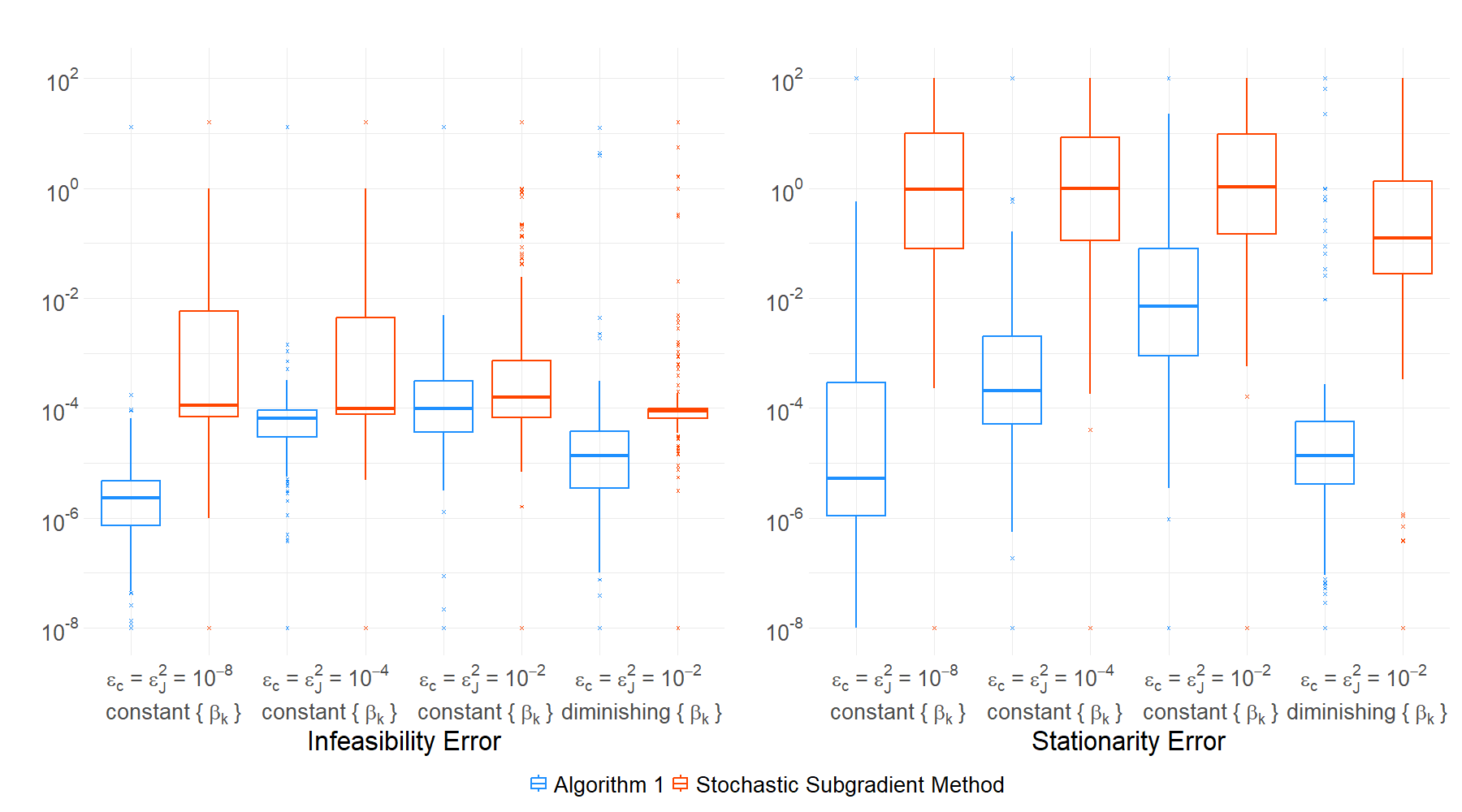
Figure 1: Box plots of infeasibility errors (the left column) and stationarity errors (the right column) on a total of 44 CUTEst problems with $\epsilon_{g}\in\{10^{-8},10^{-4},10^{-2}\}$ (from top to bottom).

Figure 1 reports box plots that include information of infeasibility errors and stationarity errors of the best iterates ever found by Algorithm 1 and the stochastic subgradient method on 44 CUTEst problems [34]. From these box plots, we observe that although provided with less CPU time, Algorithm 1 constantly outperforms the stochastic subgradient method in terms of both infeasibility error and stationarity error over all options of variance level $(\epsilon_{g},\epsilon_{c},\epsilon_{J})$ and step size parameter sequence $\{\beta_{k}\}$. In particular, Algorithm 1 is usually able to identify the best iterate with infeasibility error smaller than $10^{-4}$ and stationarity error smaller than $10^{-2}$, while the stochastic subgradient method suffers from improving stationarity errors. In addition, by comparing results over different sample variances, we notice that Algorithm 1 can achieve better iterates, in terms of both infeasibility errors and stationarity errors, when the variance level $(\epsilon_{g},\epsilon_{c},\epsilon_{J})$ is smaller, which matches the result of Case (i) of Corollary 1 that the upper bound of convergence neighborhood decays as the variances diminish. Last but not least, we know from these box plots that both Algorithm 1 and the stochastic subgradient method may benefit from utilizing a diminishing $\{\beta_{k}\}$ sequence, which controls step sizes and variances of stochastic objective gradient, constraint function, and constraint jacobian estimates. This result has also been described by Corollary 1 that a constant $\{\beta_{k}\}$ sequence can make Algorithm 1 converge to a neighborhood of stationarity in expectation (see Case (i) of Corollary 1) while a diminishing sequence of $\{\beta_{k}\}$ would enhance the performance of Algorithm 1 to exact convergence in expectation (Case (ii) of Corollary 1).

5.2 Experiments on LIBSVM [14] problems

In the second set of experiments, we tested the performance of our proposed Algorithm 1 against with TStoM, a stochastic momentum-based optimization algorithm designed by [17]. We especially considered the following constrained binary classification problem:

$$\mathop{\text{min}}\limits_{x\in\mathbb{R}^{n}}f(x)=\frac{1}{N}\sum\limits_{i=1}^{N}\text{log}(1+e^{-y_{i}(X_{i}^{T}x)})\text{ s.t. }\frac{1}{K}\sum\limits_{k=1}^{K}A_{1,k}x=\frac{1}{K}\sum\limits_{k=1}^{K}a_{1,k},||x||_{2}^{2}=a_{2},$$ (77)

where $X_{i}\in\mathbb{R}^{n}$ and $y_{i}\in\{-1,1\}$ are data representing the feature vector and the label, respectively, for each $i\in[N]$; $K=1000$, $a_{2}=1$, and $(A_{1,k},a_{1,k})\in\mathbb{R}^{10\times n}\times\mathbb{R}^{10}$ are random matrices and random vectors for each $k\in[K]$. Each random matrix $A_{1,k}$ was generated based on a fixed matrix $A_{1}\in\mathbb{R}^{10\times n}$ that $A_{1,k}^{(i,j)}$, the element at $i$th row and $j$th column of $A_{1,k}$, satisfied $A_{1,k}^{(i,j)}\sim\mathcal{N}\left(A_{1}^{(i,j)},\frac{10^{-3}}{n}\right)$ with $A_{1}^{(i,j)}\sim\mathcal{N}(1,100)$ for any $(i,j,k)\in[10]\times[n]\times[1000]$, i.e., each element of the fixed matrix $A_{1}$ was generated by the distribution of $\mathcal{N}(1,100)$ and each element of $A_{1,k}$ followed a normal distribution with the mean value as the corresponding element of $A_{1}$ and the variance as $\frac{10^{-3}}{n}$. Similarly, we first generated a fixed vector $a_{1}\in\mathbb{R}^{10}$, whose elements all followed the distribution of $\mathcal{N}(1,100)$, then each random vector $a_{1,k}\in\mathbb{R}^{10}$ was sampled by using $a_{1,k}\sim\mathcal{N}(a_{1},10^{-3}I)$ for any $k\in[1000]$. We tested problem (77) over five datasets from the LIBSVM collection [14] with five independent runs, while the dataset information is listed in Table 1.

Table 1: Binary classification datasets details. For more information, see [14]

Dataset	Dimension ($n$)	$\#$ of Data ($N$)
a9a	123	32,561
ionosphere	34	351
mushrooms	112	5,500
phishing	68	11,055
sonar	60	208

At the beginning of each run of Algorithm 1 and TStoM [17], we selected the objective batch size $b_{1}$ and the constraint batch size $b_{2}$, where $(b_{1},b_{2})\in\{16,128\}\times\{16,128\}$. For all instances, we initialized $x_{1}\in\mathbb{R}^{n}$ by sampling from the standard Gaussian distribution and normalizing it to ensure $\|x_{1}\|=0.1$. Based on the structure of problem (77), we set $\Gamma=2$ and estimated $L$ using differences of gradients near $x_{1}$. With exceptions of Lipschitz constants $(L,\Gamma)$ described above and step size parameters $\beta_{k}=1$ for all iterations $k\in\mathbb{N}$, all other parameter selections of Algorithm 1 were the same with experiments conducted in Section 5.1. For TStoM, we set $T=10$, $\gamma=0.3$, and $V=2\times 10^{7}$ for Phase I iterations and $\alpha_{k}=0.6$, $\tau_{k}=0.3$, $\beta_{k}=50$, $\eta_{k}=0.0005$, $\rho_{k}=0.5$ for Phase II iterations, as suggested by the authors of [17]. We first ran each instance of Algorithm 1 with 1000 iterations, and then provided the same amount of CPU time that had been used by Algorithm 1 to all TStoM [17] instances. After finishing all runs of both algorithms, following the same policies in Section 5.1, we selected the best iterates ever found by Algorithm 1 and TStoM [17] and reported their infeasibility errors and stationarity errors in Table 2.

Table 2: Mean values of infeasibility error and stationarity error of Algorithm 1 and TStoM [17]

	$b_{1}=16$, $b_{2}=16$				$b_{1}=16$, $b_{2}=128$
	Infeasibility Error		Stationarity Error		Infeasibility Error		Stationarity Error
Dataset	Algorithm 1	TStoM	Algorithm 1	TStoM	Algorithm 1	TStoM	Algorithm 1	TStoM
a9a	$6.12e$-05	$2.99e$-01	$2.23e$-05	$1.88e$-05	$4.65e$-05	$2.27e$-01	$2.29e$-05	$1.85e$-05
ionosphere	$6.51e$-05	$6.20e$-02	$8.79e$-04	$1.04e$-03	$6.82e$-05	$9.57e$-02	$6.89e$-04	$1.75e$-03
mushrooms	$9.05e$-06	$5.94e$-03	$1.02e$-04	$1.38e$-04	$9.13e$-06	$2.71e$-01	$8.59e$-05	$1.90e$-04
phishing	$2.53e$-05	$8.19e$-02	$1.20e$-05	$1.18e$-05	$1.37e$-05	$2.84e$-01	$1.19e$-05	$1.03e$-05
sonar	$8.49e$-05	$4.71e$-02	$3.66e$-03	$3.78e$-03	$6.29e$-05	$2.36e$-01	$3.59e$-03	$2.74e$-03
	$b_{1}=128$, $b_{2}=16$				$b_{1}=128$, $b_{2}=128$
	Infeasibility Error		Stationarity Error		Infeasibility Error		Stationarity Error
Dataset	Algorithm 1	TStoM	Algorithm 1	TStoM	Algorithm 1	TStoM	Algorithm 1	TStoM
a9a	$1.85e$-05	$2.99e$-01	$1.87e$-05	$1.88e$-05	$1.68e$-05	$2.27e$-01	$1.87e$-05	$1.84e$-05
ionosphere	$1.53e$-05	$6.20e$-02	$6.11e$-04	$1.51e$-03	$1.35e$-05	$9.57e$-02	$1.99e$-04	$1.76e$-03
mushrooms	$6.84e$-06	$6.88e$-03	$2.34e$-05	$1.75e$-04	$5.30e$-06	$2.71e$-01	$8.86e$-06	$1.91e$-04
phishing	$9.94e$-06	$8.19e$-02	$1.16e$-05	$1.18e$-05	$9.73e$-06	$2.84e$-01	$1.15e$-05	$1.03e$-05
sonar	$6.18e$-05	$4.73e$-02	$3.72e$-03	$3.79e$-03	$3.11e$-05	$2.36e$-01	$3.59e$-03	$2.74e$-03

From Table 2, we find that given the same CPU time budget, Algorithm 1 could determine near-feasible and near-stationary iterates for almost all instances over different datasets and various combinations of batch sizes on objective and constraint functions, while TStoM [17] struggled for identifying a near-feasible solution. For example, when $(b_{1},b_{2})=(16,16)$, Table 2 shows that Algorithm 1 achieved best iterates with averaged infeasibility error and stationarity error at the order of 1e-05 and 1e-04, respectively, while TStoM [17] only attained an averaged infeasibility error at the order of 1e-02, which was not even close to feasibility, making stationarity errors meaningless. Additionally, we can conclude from Table 2 that larger batch sizes tend to improve the performance of Algorithm 1, while such relations are not clear for TStoM [17] instances. This observation shows the efficiency and efficacy of Algorithm 1, while the performance of TStoM [17] could heavily rely on the selection of input parameters, where problem-dependent heavy tuning processes might be necessary to guarantee the robustness of the algorithm.

6 Conclusion

In this paper, we discuss the design, analysis, and implementation of a stochastic SQP algorithm for solving expectation-equality-constrained stochastic optimization problems. Our algorithm is objective-function-free that its iterative update only relies on the estimates of objective gradient, constraint function, and constraint jacobian information. Meanwhile, we consider the “fully-stochastic” regime that only relatively loose conditions on the quality of stochastic estimates need to be satisfied at each iteration. Our proposed algorithm does not require a heavy-tuning process, as it utilizes adaptive parameter and step size update strategies. Under common assumptions, we have shown that our algorithm achieves theoretical convergence guarantees and both iteration and sample complexity results in expectation. These theoretical results all match the performance of corresponding state-of-the-art unconstrained stochastic optimization algorithms. The results of numerical experiments have shown that our proposed stochastic SQP algorithm is more efficient and more reliable than a stochastic subgradient method and a stochastic momentum-based algorithm on classic constrained optimization test problems.

Appendix A Proof of Lemma 10

Proof of Lemma 10.

To simplify notations, we denote $A_{k}:=\begin{bmatrix}H_{k}&\nabla c(X_{k})\\ \nabla c(X_{k})^{T}&0\end{bmatrix}$ and $\bar{A}_{k}:=\begin{bmatrix}H_{k}&\bar{J}_{k}^{T}\\ \bar{J}_{k}&0\end{bmatrix}$ for each iteration $k$. By triangle inequality and Lemma 1, for any $k\in\mathbb{N}$,

$$\lVert\bar{A}_{k}^{-1}-A_{k}^{-1}\rVert\leq\|\bar{A}_{k}^{-1}\|+\|A_{k}^{-1}\|\leq\frac{2}{q_{\mathop{\textrm{min}}}},$$

which proves the first part of the statement. Moreover, when $\|\bar{A}_{k}-A_{k}\|<\frac{q_{\mathop{\textrm{min}}}}{3}$, using the Cauchy–Schwarz inequality and Lemma 1, we know

$$\|A_{k}^{-1}(\bar{A}_{k}-A_{k})\|\leq\|A_{k}^{-1}\|\|\bar{A}_{k}-A_{k}\|\leq\frac{1}{q_{\mathop{\textrm{min}}}}\cdot\frac{q_{\mathop{\textrm{min}}}}{3}=\frac{1}{3}.$$ (78)

Furthermore, for any $k\in\mathbb{N}$,

$$\bar{A}_{k}^{-1} =(A_{k}+(\bar{A}_{k}-A_{k}))^{-1}=(A_{k}(I+A_{k}^{-1}(\bar{A}_{k}-A_{k})))^{-1}$$

$$=(I+A_{k}^{-1}(\bar{A}_{k}-A_{k}))^{-1}A_{k}^{-1}=\left(I+\sum_{j=1}^{\infty}(-1)^{j}(A_{k}^{-1}(\bar{A}_{k}-A_{k}))^{j}\right)A_{k}^{-1},$$

where the last equality follows [1, Proposition 3.3.1]. Meanwhile, by triangle inequality and Lemma 1, we have that

$$\|\bar{A}_{k}^{-1}-A_{k}^{-1}\| =\left\|\left(\sum_{j=1}^{\infty}(-1)^{j}(A_{k}^{-1}(\bar{A}_{k}-A_{k}))^{j}\right)A_{k}^{-1}\right\|\leq\left\|\sum_{j=1}^{\infty}(-1)^{j}(A_{k}^{-1}(\bar{A}_{k}-A_{k}))^{j}\right\|\cdot\|A_{k}^{-1}\|$$

$$\leq\frac{1}{q_{\mathop{\textrm{min}}}}\cdot\sum_{j=1}^{\infty}\left\|A_{k}^{-1}(\bar{A}_{k}-A_{k})\right\|^{j}=\frac{1}{q_{\mathop{\textrm{min}}}}\cdot\frac{\|A_{k}^{-1}(\bar{A}_{k}-A_{k})\|}{1-\|A_{k}^{-1}(\bar{A}_{k}-A_{k})\|}\leq\frac{3\|A_{k}^{-1}(\bar{A}_{k}-A_{k})\|}{2q_{\mathop{\textrm{min}}}}$$

$$\leq\frac{3\|A_{k}^{-1}\|\|\bar{A}_{k}-A_{k}\|}{2q_{\mathop{\textrm{min}}}}\leq\frac{3}{2q_{\mathop{\textrm{min}}}^{2}}\cdot\|\bar{A}_{k}-A_{k}\|,$$

where the second equality and the third inequality are both from (78). ∎

Appendix B Proof of Lemma 11

Proof of Lemma 11..

Similar to the proof of Lemma 10, we first define matrices $A_{k}:=\begin{bmatrix}H_{k}&\nabla c(X_{k})\\ \nabla c(X_{k})^{T}&0\end{bmatrix}$ and $\bar{A}_{k}:=\begin{bmatrix}H_{k}&\bar{J}_{k}^{T}\\ \bar{J}_{k}&0\end{bmatrix}$ for all iterations $k$ to simplify notations. By (6) and (15), it holds that for any $k\in\mathbb{N}{}$,

$$\begin{bmatrix}\bar{D}_{k}\\ \bar{Y}_{k}\end{bmatrix}-\begin{bmatrix}D_{k}\\ Y_{k}\end{bmatrix}=-\bar{A}_{k}^{-1}\begin{bmatrix}\bar{G}_{k}\\ \bar{C}_{k}\end{bmatrix}+A_{k}^{-1}\begin{bmatrix}\nabla f(X_{k})\\ c(X_{k})\end{bmatrix}=(A_{k}^{-1}-\bar{A}_{k}^{-1})\begin{bmatrix}\bar{G}_{k}\\ \bar{C}_{k}\end{bmatrix}+A_{k}^{-1}\begin{bmatrix}\nabla f(X_{k})-\bar{G}_{k}\\ c(X_{k})-\bar{C}_{k}\end{bmatrix}.$$

Next, for every iteration $k\in\mathbb{N}{}$, we define the following events depending on whether $\bar{A}_{k}$ and $A_{k}$ are close enough, i.e., let $E_{k}$ be the event that $\|\bar{A}_{k}-A_{k}\|<\frac{q_{\mathop{\textrm{min}}}}{3}$ and let $E_{k}^{c}$ be the event that $\|\bar{A}_{k}-A_{k}\|\geq\frac{q_{\mathop{\textrm{min}}}}{3}$. Furthermore, using conditional Markov’s inequality, we have that

$$\mathbb{P}_{k}[E_{k}^{c}] =\mathbb{P}_{k}\left[\|\bar{A}_{k}-A_{k}\|\geq\frac{q_{\mathop{\textrm{min}}}}{3}\right]\leq\frac{9\mathbb{E}_{k}\left[\|\bar{A}_{k}-A_{k}\|^{2}\right]}{q_{\mathop{\textrm{min}}}^{2}}\leq\frac{9\mathbb{E}_{k}\left[\|\bar{A}_{k}-A_{k}\|_{F}^{2}\right]}{q_{\mathop{\textrm{min}}}^{2}}$$ (79)

$$=\frac{18\mathbb{E}_{k}\left[\|\bar{J}_{k}-\nabla c(X_{k})^{T}\|_{F}^{2}\right]}{q_{\mathop{\textrm{min}}}^{2}}\leq\frac{18\rho_{k}^{j}}{q_{\mathop{\textrm{min}}}^{2}},$$

where the last inequality follows (25). Consequently, by Lemma 10 and triangle inequality, we further have

$$\mathbb{E}_{k}\left[\|\bar{A}_{k}^{-1}-A_{k}^{-1}\|\right] =\mathbb{E}_{k}\left[\|\bar{A}_{k}^{-1}-A_{k}^{-1}\||E_{k}\right]\cdot\mathbb{P}_{k}[E_{k}]+\mathbb{E}_{k}\left[\|\bar{A}_{k}^{-1}-A_{k}^{-1}\||E_{k}^{c}\right]\cdot\mathbb{P}_{k}[E_{k}^{c}]$$ (80)

$$\leq\frac{3}{2q_{\mathop{\textrm{min}}}^{2}}\cdot\mathbb{E}_{k}\left[\|\bar{A}_{k}-A_{k}\||E_{k}\right]\cdot\mathbb{P}_{k}[E_{k}]+\mathbb{E}_{k}\left[\|\bar{A}_{k}^{-1}\|+\|A_{k}^{-1}\||E_{k}^{c}\right]\cdot\mathbb{P}_{k}[E_{k}^{c}]$$

$$\leq\frac{3}{2q_{\mathop{\textrm{min}}}^{2}}\cdot\mathbb{E}_{k}\left[\|\bar{A}_{k}-A_{k}\|\right]+\frac{2}{q_{\mathop{\textrm{min}}}}\cdot\mathbb{P}_{k}[E_{k}^{c}]\leq\frac{3}{2q_{\mathop{\textrm{min}}}^{2}}\cdot\sqrt{\mathbb{E}_{k}\left[\|\bar{A}_{k}-A_{k}\|_{F}^{2}\right]}+\frac{36\rho_{k}^{j}}{q_{\mathop{\textrm{min}}}^{3}}$$

$$=\frac{3}{\sqrt{2}q_{\mathop{\textrm{min}}}^{2}}\cdot\sqrt{\mathbb{E}_{k}\left[\|\bar{J}_{k}-\nabla c(X_{k})^{T}\|_{F}^{2}\right]}+\frac{36\rho_{k}^{j}}{q_{\mathop{\textrm{min}}}^{3}}\leq\frac{3\sqrt{\rho_{k}^{j}}}{\sqrt{2}q_{\mathop{\textrm{min}}}^{2}}+\frac{36\rho_{k}^{j}}{q_{\mathop{\textrm{min}}}^{3}},$$

where the second inequality follows Lemma 1, the third inequality is using (79), the second equality comes from the structure of $\bar{A}_{k}$ and $A_{k}$, and the last inequality is from Assumption 5. Now we are ready to show the main results in the statement.

First, for any iteration $k\in\mathbb{N}{}$, it follows (6), (15), Assumption 5, and the Cauchy–Schwarz inequality that

$$\left\|\mathbb{E}_{k}\left[\bar{D}_{k}-D_{k}\right]\right\| \leq\left\|\mathbb{E}_{k}\left[\begin{bmatrix}\bar{D}_{k}\\ \bar{Y}_{k}\end{bmatrix}-\begin{bmatrix}D_{k}\\ Y_{k}\end{bmatrix}\right]\right\|=\left\|\mathbb{E}_{k}\left[\bar{A}_{k}^{-1}\begin{bmatrix}\bar{G}_{k}\\ \bar{C}_{k}\end{bmatrix}-A_{k}^{-1}\begin{bmatrix}\nabla f(X_{k})\\ c(X_{k})\end{bmatrix}\right]\right\|$$

$$=\left\|\mathbb{E}_{k}\left[(\bar{A}_{k}^{-1}-A_{k}^{-1})\begin{bmatrix}\bar{G}_{k}\\ \bar{C}_{k}\end{bmatrix}\right]\right\|=\left\|\mathbb{E}_{k}\left[\bar{A}_{k}^{-1}-A_{k}^{-1}\right]\cdot\mathbb{E}_{k}\begin{bmatrix}\begin{bmatrix}\bar{G}_{k}\\ \bar{C}_{k}\end{bmatrix}\end{bmatrix}\right\|$$

$$\leq\left\|\mathbb{E}_{k}\left[\bar{A}_{k}^{-1}-A_{k}^{-1}\right]\right\|\cdot\left\|\mathbb{E}_{k}\begin{bmatrix}\begin{bmatrix}\bar{G}_{k}\\ \bar{C}_{k}\end{bmatrix}\end{bmatrix}\right\|=\left\|\mathbb{E}_{k}\left[\bar{A}_{k}^{-1}-A_{k}^{-1}\right]\right\|\cdot\left\|\begin{bmatrix}\nabla f(X_{k})\\ c(X_{k})\end{bmatrix}\right\|$$

$$\leq\mathbb{E}_{k}\left[\left\|\bar{A}_{k}^{-1}-A_{k}^{-1}\right\|\right]\cdot(\kappa_{\nabla f}+\kappa_{c})\leq\frac{\kappa_{\nabla f}+\kappa_{c}}{q_{\mathop{\textrm{min}}}^{3}}\cdot\left(\frac{3}{\sqrt{2}}q_{\mathop{\textrm{min}}}\sqrt{\rho_{k}^{j}}+36\rho_{k}^{j}\right),$$

where the third equality follows from the assumed independence between $\bar{J}_{k}$ and $(\bar{G}_{k},\bar{C}_{k})$ in Assumption 5, the second last inequality is from (3), and the last inequality follows (80). Because $\rho_{k}^{j}\leq\sqrt{\rho_{\text{max}}}\cdot\sqrt{\rho_{k}^{j}}$ for all $k\in\mathbb{N}{}$ (see Assumption 5), by setting the fixed constant $\omega_{1}:=\frac{\kappa_{\nabla f}+\kappa_{c}}{q_{\mathop{\textrm{min}}}^{3}}\cdot\left(\frac{3}{\sqrt{2}}q_{\mathop{\textrm{min}}}+36\sqrt{\rho_{\text{max}}}\right)$, we may conclude the first part of the statement.

Meanwhile, for any iteration $k\in\mathbb{N}{}$, using (6), (15), Assumption 5, and the Cauchy–Schwarz inequality, we have

$$\mathbb{E}_{k}\left[\|\bar{D}_{k}-D_{k}\|\right] \leq\mathbb{E}_{k}\left[\left\|\begin{bmatrix}\bar{D}_{k}\\ \bar{Y}_{k}\end{bmatrix}-\begin{bmatrix}D_{k}\\ Y_{k}\end{bmatrix}\right\|\right]=\mathbb{E}_{k}\left[\left\|\bar{A}_{k}^{-1}\begin{bmatrix}\bar{G}_{k}\\ \bar{C}_{k}\end{bmatrix}-A_{k}^{-1}\begin{bmatrix}\nabla f(X_{k})\\ c(X_{k})\end{bmatrix}\right\|\right]$$

$$\leq\mathbb{E}_{k}\left[\left\|\bar{A}_{k}^{-1}\begin{bmatrix}\bar{G}_{k}-\nabla f(X_{k})\\ \bar{C}_{k}-c(X_{k})\end{bmatrix}\right\|\right]+\mathbb{E}_{k}\left[\left\|(\bar{A}_{k}^{-1}-A_{k}^{-1})\begin{bmatrix}\nabla f(X_{k})\\ c(X_{k})\end{bmatrix}\right\|\right]$$

$$\leq\mathbb{E}_{k}\left[\left\|\bar{A}_{k}^{-1}\right\|\cdot\left\|\begin{bmatrix}\bar{G}_{k}-\nabla f(X_{k})\\ \bar{C}_{k}-c(X_{k})\end{bmatrix}\right\|\right]+\mathbb{E}_{k}\left[\left\|\bar{A}_{k}^{-1}-A_{k}^{-1}\right\|\right]\cdot\left\|\begin{bmatrix}\nabla f(X_{k})\\ c(X_{k})\end{bmatrix}\right\|$$

$$\leq\frac{1}{q_{\mathop{\textrm{min}}}}\cdot\mathbb{E}_{k}\left[\left\|\begin{bmatrix}\bar{G}_{k}-\nabla f(X_{k})\\ \bar{C}_{k}-c(X_{k})\end{bmatrix}\right\|\right]+(\kappa_{\nabla f}+\kappa_{c})\cdot\mathbb{E}_{k}\left[\left\|\bar{A}_{k}^{-1}-A_{k}^{-1}\right\|\right]$$

$$\leq\frac{1}{q_{\mathop{\textrm{min}}}}\cdot\sqrt{\mathbb{E}_{k}\left[\left\|\begin{bmatrix}\bar{G}_{k}-\nabla f(X_{k})\\ \bar{C}_{k}-c(X_{k})\end{bmatrix}\right\|^{2}\right]}+(\kappa_{\nabla f}+\kappa_{c})\cdot\mathbb{E}_{k}\left[\left\|\bar{A}_{k}^{-1}-A_{k}^{-1}\right\|\right]$$

$$\leq\frac{\sqrt{\rho_{k}^{g}+\rho_{k}^{c}}}{q_{\mathop{\textrm{min}}}}+\frac{\kappa_{\nabla f}+\kappa_{c}}{q_{\mathop{\textrm{min}}}^{3}}\cdot\left(\frac{3}{\sqrt{2}}q_{\mathop{\textrm{min}}}\sqrt{\rho_{k}^{j}}+36\rho_{k}^{j}\right)\leq\frac{\sqrt{\rho_{k}^{g}+\rho_{k}^{c}}}{q_{\mathop{\textrm{min}}}}+\omega_{1}\cdot\sqrt{\rho_{k}^{j}},$$

where the fourth inequality is from Lemma 1 and (3), the second last inequality follows Assumption 5 and (80), and the last inequality relies on the definition of $\omega_{1}$, which is defined in the first part of the proof, and $\rho_{k}^{j}\leq\sqrt{\rho_{\text{max}}}\cdot\sqrt{\rho_{k}^{j}}$ at any iteration $k\in\mathbb{N}{}$ (see Assumption 5). Therefore, we conclude the statement. ∎

Appendix C Proof of Lemma 12

Proof of Lemma 12..

Similar to the proof of Lemma 10, we first define matrices $A_{k}:=\begin{bmatrix}H_{k}&\nabla c(X_{k})\\ \nabla c(X_{k})^{T}&0\end{bmatrix}$ and $\bar{A}_{k}:=\begin{bmatrix}H_{k}&\bar{J}_{k}^{T}\\ \bar{J}_{k}&0\end{bmatrix}$ for all iterations $k$ to simplify notations. By (6) and (15), it holds that for any $k\in\mathbb{N}{}$,

$$\mathbb{E}_{k}\left[\left\|\bar{D}_{k}-D_{k}\right\|^{2}\right] \leq\mathbb{E}_{k}\left[\left\|\begin{bmatrix}\bar{D}_{k}\\ \bar{Y}_{k}\end{bmatrix}-\begin{bmatrix}D_{k}\\ Y_{k}\end{bmatrix}\right\|^{2}\right]=\mathbb{E}_{k}\left[\left\|\bar{A}_{k}^{-1}\begin{bmatrix}\bar{G}_{k}\\ \bar{C}_{k}\end{bmatrix}-A_{k}^{-1}\begin{bmatrix}\nabla f(X_{k})\\ c(X_{k})\end{bmatrix}\right\|^{2}\right]{}$$

$$=\mathbb{E}_{k}\left[\left\|\bar{A}_{k}^{-1}\begin{bmatrix}\bar{G}_{k}-\nabla f(X_{k})\\ \bar{C}_{k}-c(X_{k})\end{bmatrix}+(\bar{A}_{k}^{-1}-A_{k}^{-1})\begin{bmatrix}\nabla f(X_{k})\\ c(X_{k})\end{bmatrix}\right\|^{2}\right]{}$$

$$=\mathbb{E}_{k}\left[\left\|\bar{A}_{k}^{-1}\begin{bmatrix}\bar{G}_{k}-\nabla f(X_{k})\\ \bar{C}_{k}-c(X_{k})\end{bmatrix}\right\|^{2}\right]+\mathbb{E}_{k}\left[\left\|(\bar{A}_{k}^{-1}-A_{k}^{-1})\begin{bmatrix}\nabla f(X_{k})\\ c(X_{k})\end{bmatrix}\right\|^{2}\right]$$ (81)

$$\quad\quad+\mathbb{E}_{k}\left[2\begin{bmatrix}\nabla f(X_{k})\\ c(X_{k})\end{bmatrix}^{T}(\bar{A}_{k}^{-1}-A_{k}^{-1})\bar{A}_{k}^{-1}\begin{bmatrix}\bar{G}_{k}-\nabla f(X_{k})\\ \bar{C}_{k}-c(X_{k})\end{bmatrix}\right].{}$$

Then we provide seperate upper bounds for the three terms on the right-hand side of (81).

First, by the Cauchy–Schwarz inequality, Lemma 1 and Assumption 5, we have

$$\mathbb{E}_{k}\left[\left\|\bar{A}_{k}^{-1}\begin{bmatrix}\bar{G}_{k}-\nabla f(X_{k})\\ \bar{C}_{k}-c(X_{k})\end{bmatrix}\right\|^{2}\right] \leq\mathbb{E}_{k}\left[\left\|\bar{A}_{k}^{-1}\right\|^{2}\cdot\left\|\begin{bmatrix}\bar{G}_{k}-\nabla f(X_{k})\\ \bar{C}_{k}-c(X_{k})\end{bmatrix}\right\|^{2}\right]$$ (82)

$$\leq\frac{1}{q_{\mathop{\textrm{min}}}^{2}}\cdot\mathbb{E}_{k}\left[\left\|\begin{bmatrix}\bar{G}_{k}-\nabla f(X_{k})\\ \bar{C}_{k}-c(X_{k})\end{bmatrix}\right\|^{2}\right]\leq\frac{\rho_{k}^{g}+\rho_{k}^{c}}{q_{\mathop{\textrm{min}}}^{2}}.$$

Before providing an upper bound for the second term, we try to bound $\mathbb{E}_{k}\left[\|\bar{A}_{k}^{-1}-A_{k}^{-1}\|^{2}\right]$ as follows. Using the same definition of events $E_{k}$ and $E_{k}^{c}$ from the proof of Lemma 11 and following the same logic as (80), by Lemma 10 and the triangle inequality, we have

$$\mathbb{E}_{k}\left[\|\bar{A}_{k}^{-1}-A_{k}^{-1}\|^{2}\right] =\mathbb{E}_{k}\left[\|\bar{A}_{k}^{-1}-A_{k}^{-1}\|^{2}|E_{k}\right]\cdot\mathbb{P}_{k}[E_{k}]+\mathbb{E}_{k}\left[\|\bar{A}_{k}^{-1}-A_{k}^{-1}\|^{2}|E_{k}^{c}\right]\cdot\mathbb{P}_{k}[E_{k}^{c}]$$ (83)

$$\leq\frac{9}{4q_{\mathop{\textrm{min}}}^{4}}\cdot\mathbb{E}_{k}\left[\|\bar{A}_{k}-A_{k}\|^{2}|E_{k}\right]\cdot\mathbb{P}_{k}[E_{k}]+\mathbb{E}_{k}\left[(\|\bar{A}_{k}^{-1}\|+\|A_{k}^{-1}\|)^{2}|E_{k}^{c}\right]\cdot\mathbb{P}_{k}[E_{k}^{c}]$$

$$\leq\frac{9}{4q_{\mathop{\textrm{min}}}^{4}}\cdot\mathbb{E}_{k}\left[\|\bar{A}_{k}-A_{k}\|^{2}\right]+\frac{4}{q_{\mathop{\textrm{min}}}^{2}}\cdot\mathbb{P}_{k}[E_{k}^{c}]$$

$$\leq\frac{9}{4q_{\mathop{\textrm{min}}}^{4}}\cdot\mathbb{E}_{k}\left[\|\bar{A}_{k}-A_{k}\|_{F}^{2}\right]+\frac{72\rho_{k}^{j}}{q_{\mathop{\textrm{min}}}^{4}}$$

$$=\frac{9}{2q_{\mathop{\textrm{min}}}^{4}}\cdot\mathbb{E}_{k}\left[\|\bar{J}_{k}-\nabla c(X_{k})^{T}\|_{F}^{2}\right]+\frac{72\rho_{k}^{j}}{q_{\mathop{\textrm{min}}}^{4}}$$

$$\leq\frac{9\rho_{k}^{j}}{2q_{\mathop{\textrm{min}}}^{4}}+\frac{72\rho_{k}^{j}}{q_{\mathop{\textrm{min}}}^{4}}=\frac{153\rho_{k}^{j}}{2q_{\mathop{\textrm{min}}}^{4}},$$

where the second inequality follows Lemma 1, the third inequality is using (79), the second equality comes from the structure of $\bar{A}_{k}$ and $A_{k}$, and the last inequality is from Assumption 5. Now from the Cauchy–Schwarz inequality, (3) and (83), we can bound the second term on the right hand side of (81) as

$$\mathbb{E}_{k}\left[\left\|(\bar{A}_{k}^{-1}-A_{k}^{-1})\begin{bmatrix}\nabla f(X_{k})\\ c(X_{k})\end{bmatrix}\right\|^{2}\right]\leq\mathbb{E}_{k}\left[\left\|\bar{A}_{k}^{-1}-A_{k}^{-1}\right\|^{2}\right]\cdot\left\|\begin{bmatrix}\nabla f(X_{k})\\ c(X_{k})\end{bmatrix}\right\|^{2}\leq\frac{153\rho_{k}^{j}}{2q_{\mathop{\textrm{min}}}^{4}}\cdot(\kappa_{\nabla f}+\kappa_{c})^{2}.$$ (84)

Lastly, to bound the last term on the right hand side of (81), it follows the Cauchy–Schwarz inequality, (3), Lemma 1, Assumption 5 and (80) that

$$\mathbb{E}_{k} \left[2\begin{bmatrix}\nabla f(X_{k})\\ c(X_{k})\end{bmatrix}^{T}(\bar{A}_{k}^{-1}-A_{k}^{-1})\bar{A}_{k}^{-1}\begin{bmatrix}\bar{G}_{k}-\nabla f(X_{k})\\ \bar{C}_{k}-c(X_{k})\end{bmatrix}\right]{}$$

$$\quad\leq 2\left\|\begin{bmatrix}\nabla f(X_{k})\\ c(X_{k})\end{bmatrix}\right\|\cdot\mathbb{E}_{k}\left[\left\|\bar{A}_{k}^{-1}-A_{k}^{-1}\right\|\cdot\|\bar{A}_{k}^{-1}\|\right]\cdot\mathbb{E}_{k}\left[\left\|\begin{bmatrix}\bar{G}_{k}-\nabla f(X_{k})\\ \bar{C}_{k}-c(X_{k})\end{bmatrix}\right\|\right]{}$$

$$\quad\leq 2\left(\kappa_{\nabla f}+\kappa_{c}\right)\cdot\frac{1}{q_{\mathop{\textrm{min}}}}\cdot\mathbb{E}_{k}\left[\left\|\bar{A}_{k}^{-1}-A_{k}^{-1}\right\|\right]\cdot\sqrt{\mathbb{E}_{k}\left[\left\|\begin{bmatrix}\bar{G}_{k}-\nabla f(X_{k})\\ \bar{C}_{k}-c(X_{k})\end{bmatrix}\right\|^{2}\right]}$$ (85)

$$\quad\leq\frac{2\left(\kappa_{\nabla f}+\kappa_{c}\right)}{q_{\mathop{\textrm{min}}}}\cdot\left(\frac{3\sqrt{\rho_{k}^{j}}}{\sqrt{2}q_{\mathop{\textrm{min}}}^{2}}+\frac{36\rho_{k}^{j}}{q_{\mathop{\textrm{min}}}^{3}}\right)\cdot\sqrt{\rho_{k}^{g}+\rho_{k}^{c}}{}$$

$$\quad\leq\frac{6\left(\kappa_{\nabla f}+\kappa_{c}\right)}{q_{\mathop{\textrm{min}}}^{4}}\cdot\left(\frac{q_{\mathop{\textrm{min}}}}{\sqrt{2}}+12\sqrt{\rho_{\text{max}}}\right)\cdot\sqrt{\rho_{k}^{j}(\rho_{k}^{g}+\rho_{k}^{c})},{}$$

where the last inequality follows Assumption 5 that $\rho_{k}^{j}\leq\sqrt{\rho_{\text{max}}}\cdot\sqrt{\rho_{k}^{j}}$ for all $k\in\mathbb{N}{}$. Combining (82), (84) and (85), and choosing sufficiently large values for constants $\omega_{2}$ and $\omega_{3}$, i.e.,

$$\omega_{2}:=\frac{153}{2q_{\mathop{\textrm{min}}}^{4}}\cdot(\kappa_{\nabla f}+\kappa_{c})^{2},\quad\omega_{3}:=\frac{6\left(\kappa_{\nabla f}+\kappa_{c}\right)}{q_{\mathop{\textrm{min}}}^{4}}\cdot\left(\frac{q_{\mathop{\textrm{min}}}}{\sqrt{2}}+12\sqrt{\rho_{\text{max}}}\right),$$

we conclude the first part of the statement.

Now we are ready to prove the second part of the statement. For any iteration $k\in\mathbb{N}{}$, using the triangle inequality, the fact of $\mathbb{E}_{k}[\bar{G}_{k}]=\nabla f(X_{k})$ (see Assumption 5) and the Cauchy–Schwarz inequality, we have

$$\left|\mathbb{E}_{k}\left[\bar{G}_{k}^{T}\bar{D}_{k}-\nabla f(X_{k})^{T}D_{k}\right]\right| \leq\left|\mathbb{E}_{k}\left[(\bar{G}_{k}-\nabla f(X_{k}))^{T}(\bar{D}_{k}-D_{k})\right]\right|+\left|\mathbb{E}_{k}\left[(\bar{G}_{k}-\nabla f(X_{k}))^{T}D_{k}\right]\right|$$

$$\quad\quad+\left|\mathbb{E}_{k}\left[\nabla f(X_{k})^{T}(\bar{D}_{k}-D_{k})\right]\right|$$

$$\leq\frac{1}{2}\mathbb{E}_{k}\left[\|\bar{G}_{k}-\nabla f(X_{k})\|^{2}\right]+\frac{1}{2}\mathbb{E}_{k}\left[\|\bar{D}_{k}-D_{k}\|^{2}\right]+\|\nabla f(X_{k})\|\cdot\left\|\mathbb{E}_{k}\left[\bar{D}_{k}-D_{k}\right]\right\|$$

$$\leq\frac{\rho_{k}^{g}}{2}+\frac{\rho_{k}^{g}+\rho_{k}^{c}}{2q_{\mathop{\textrm{min}}}^{2}}+\frac{\omega_{2}}{2}\cdot\rho_{k}^{j}+\frac{\omega_{3}}{2}\cdot\sqrt{\rho_{k}^{j}(\rho_{k}^{g}+\rho_{k}^{c})}+\kappa_{\nabla f}\omega_{1}\cdot\sqrt{\rho_{k}^{j}}$$

$$\leq\frac{\rho_{k}^{g}}{2}+\frac{\rho_{k}^{g}+\rho_{k}^{c}}{2q_{\mathop{\textrm{min}}}^{2}}+\omega_{4}\cdot\sqrt{\rho_{k}^{j}}+\frac{\omega_{3}}{2}\cdot\sqrt{\rho_{k}^{j}(\rho_{k}^{g}+\rho_{k}^{c})},$$

where the second last inequality comes from (3), Assumption 5, Lemma 11, and the first part of the statement in this lemma, and the last inequality follows the fact of $\rho_{k}^{j}\leq\sqrt{\rho_{\text{max}}}\cdot\sqrt{\rho_{k}^{j}}$ (see Assumption 5) and choosing a suitable value for $\omega_{4}$, e.g., $\omega_{4}=\frac{\sqrt{\rho_{\text{max}}}}{2}\omega_{2}+\kappa_{\nabla f}\omega_{1}$. Therefore, the proof is completed. ∎

Appendix D Proof of Lemma 15

The proof of Lemma 15 relies on the following lemmas. We first show that the function $T_{d}$ is Lipschitz continuous, which helps to bound the difference between $T_{d}(Z_{k}+\bar{\Delta}_{k},H_{k})$ and $T_{d}(Z_{k},H_{k})$ using $\lVert\bar{\Delta}_{k}\rVert$.

Lemma 28.

Given any constant $\Lambda>0$, $f(x,Y):=x^{T}Y^{-1}x$ is Lipschitz continuous on $\mathcal{S}_{\Lambda}:=\{(x,Y)\in\mathbb{R}^{n}\times\mathbb{S}^{n}:\|x\|\leq\Lambda,Y^{T}Y\succeq\frac{1}{\Lambda}I\}$.

Proof of Lemma 28.

To conclude the statement, it is enough to show that there exists a constant $L>0$ such that for any $\{(x_{1},Y_{1}),(x_{2},Y_{2})\}\subset\mathcal{S}_{\Lambda}$, it always holds that

$$\lvert f(x_{1},Y_{1})-f(x_{2},Y_{2})\rvert\leq L\left(\lVert x_{1}-x_{2}\rVert+\lVert Y_{1}-Y_{2}\rVert\right).$$

We first fix $Y$ terms and compare the function values at different $x$ values. For any $\{(x_{1},Y),(x_{2},Y)\}\subset\mathcal{S}_{\Lambda}$, by the Cauchy–Schwarz inequality and the definition of $\mathcal{S}_{\Lambda}$, we have

$$\lvert f(x_{1},Y)-f(x_{2},Y)\rvert =\lvert x_{1}^{T}Y^{-1}x_{1}-x^{T}_{2}Y^{-1}x_{2}\rvert=\lvert(x_{1}+x_{2})^{T}Y^{-1}(x_{1}-x_{2})\rvert$$

$$\leq\lVert x_{1}+x_{2}\rVert\cdot\lVert Y^{-1}\rVert\cdot\lVert x_{1}-x_{2}\rVert\leq 2\Lambda^{\frac{3}{2}}\cdot\|x_{1}-x_{2}\|\leq L_{x}\lVert x_{1}-x_{2}\rVert$$

for some large enough constant $L_{x}\geq 2\Lambda^{\frac{3}{2}}$. Next, we bound the partial derivative of $f(x,Y)$ with respect to $Y$ for any fixed $x$. Specifically, by [50, Equation (61)], the Cauchy-Schwarz inequality, and a large enough constant $L_{Y}\geq\Lambda^{3}$, we have

$$\lVert\partial_{Y}f(x,Y)\rVert=\lVert-Y^{-T}xx^{T}Y^{-T}\rVert\leq\lVert xx^{T}\rVert\lVert Y^{-T}\rVert^{2}\leq\|x\|^{2}\|Y^{-1}\|^{2}\leq\Lambda^{3}\leq L_{Y}.$$

Therefore, by the triangle inequality, it holds that

$$\lvert f(x_{1},Y_{1})-f(x_{2},Y_{2})\rvert\leq\lvert f(x_{1},Y_{1})-f(x_{1},Y_{2})\rvert+\lvert f(x_{1},Y_{2})-f(x_{2},Y_{2})\rvert\leq L_{Y}\|Y_{1}-Y_{2}\|+L_{x}\|x_{1}-x_{2}\|,$$

and we conclude the proof by taking $L=\mathop{\textrm{max}}\{L_{x},L_{Y}\}>0$. ∎

We then establish a useful probability inequality in Lemma 30, building on the fundamental Markov-type probabilistic inequality provided in Lemma 29.

Lemma 29.

Suppose that $X\in\mathbb{R}$ is a random variable with $\mathbb{E{}}\left[X^{2}\right]<+\infty$ and $\mathbb{E{}}\left[X\right]>0$. Then,

$$\mathbb{P{}}\left[X>0\right]\geq\frac{\left(\mathbb{E{}}\left[X\right]\right)^{2}}{\left(\mathbb{E{}}\left[X\right]\right)^{2}+\mathop{\textbf{Var}}\left[X\right]},$$ (86)

where $\mathop{\textbf{Var}}\left[X\right]$ represents for the variance of $X$.

Proof.

To begin with, notice that $\mathbb{E{}}\left[X^{2}\right]\geq\left(\mathbb{E{}}\left[X\right]\right)^{2}>0$. Then, by the Cauchy–Schwarz inequality and properties of integration, one has

$$0<\mathbb{E{}}\left[X\right]=\mathbb{E{}}\left[X\cdot\mathbf{1}\left(X>0\right)\right]+\mathbb{E{}}\left[X\cdot\mathbf{1}\left(X\leq 0\right)\right]\leq\mathbb{E{}}\left[X\cdot\mathbf{1}\left(X>0\right)\right]\leq\sqrt{\mathbb{E{}}\left[X^{2}\right]\cdot\mathbb{P{}}\left[X>0\right]},$$

from which $\displaystyle\mathbb{P{}}[X>0]\geq\frac{\left(\mathbb{E{}}\left[X\right]\right)^{2}}{\mathbb{E{}}\left[X^{2}\right]}$, and (86) follows from $\mathop{\textbf{Var}}\left[X\right]=\mathbb{E{}}\left[X^{2}\right]-\left(\mathbb{E{}}\left[X\right]\right)^{2}$. ∎

Lemma 30.

Suppose that $\Delta$ is a random vector satisfying

$$\mathbb{E{}}\left[\Delta\right]=0,\quad 0\in\mathop{\textbf{supp}}(\Delta),\ \ \text{and}\ \ \mathbb{E{}}\left[\lVert\Delta\rVert^{2}\right]<+\infty.$$

Then, for any $\{\epsilon,M\}\subset\mathbb{R}_{>0}$, it holds for any $r\in(0,\frac{\epsilon}{2M}]$ that

$$\mathbb{P{}}\left[\epsilon-M\lVert\Delta\rVert>0\right] \geq\mathbb{P{}}\left[(\epsilon-M\lVert\Delta\rVert)\cdot\mathbf{1}\left(\lVert\Delta\rVert<r\right)>0\right]{}$$

$$\geq\frac{\mathbb{E{}}\left[\left(\epsilon-M\lVert\Delta\rVert\right)\cdot\mathbf{1}\left(\lVert\Delta\rVert<r\right)\right]}{\epsilon-M\mathbb{E{}}\left[\lVert\Delta\rVert\cdot\mathbf{1}\left(\lVert\Delta\rVert<r\right)\right]+\left(M^{2}/\epsilon\right)\mathbb{E{}}\left[\lVert\Delta\rVert^{2}\right]}.$$ (87)

Proof of Lemma 30.

Let $X:=(\epsilon-M\lVert\Delta\rVert)\cdot\mathbf{1}\left(\lVert\Delta\rVert<r\right)$. By the choice of $r$ and $0\in\mathop{\textbf{supp}}(\Delta)$, we have

$$0<\epsilon/2\cdot\mathbb{P{}}\left[\lVert\Delta\rVert<r\right]\leq\mathbb{E{}}\left[(\epsilon-M\lVert\Delta\rVert)\cdot\mathbf{1}\left(\lVert\Delta\rVert<r\right)\right],$$

and $$\mathbb{E{}}\left[(\epsilon-M\lVert\Delta\rVert)^{2}\cdot\mathbf{1}\left(\lVert\Delta\rVert<r\right)\right]\leq\epsilon^{2}<+\infty.$$

Consequently, applying Lemma 29 to $X$ yields

$$\mathbb{P{}}\left[\epsilon-M\lVert\Delta\rVert>0\right]\geq\mathbb{P{}}\left[\left(\epsilon-M\lVert\Delta\rVert\right)\cdot\mathbf{1}\left(\lVert\Delta\rVert<r\right)>0\right]=\mathbb{P{}}\left[X>0\right]\geq\frac{\left(\mathbb{E{}}\left[X\right]\right)^{2}}{\left(\mathbb{E{}}\left[X\right]\right)^{2}+\mathop{\textbf{Var}}\left[X\right]},$$ (88)

where the first inequality is because $\lVert\Delta\rVert<r\in(0,\frac{\epsilon}{2M}]$ implies $\epsilon-M\lVert\Delta\rVert>\epsilon/2>0$. Next, we will derive a lower bound for (88) by constructing an upper bound for $\mathop{\textbf{Var}}\left[X\right]$. Since $X=(\epsilon-M\lVert\Delta\rVert)\cdot\mathbf{1}{}\left(\lVert\Delta\rVert<r\right)$, one can expand $\mathop{\textbf{Var}}{}\left[X\right]$ with $X_{1}:=\epsilon\cdot\mathbf{1}{}\left(\lVert\Delta\rVert<r\right)$ and $X_{2}:=M\lVert\Delta\rVert\cdot\mathbf{1}\left(\lVert\Delta\rVert<r\right)$ as

$$\mathop{\textbf{Var}}{}\left[X\right]=\mathop{\textbf{Var}}{}\left[X_{1}-X_{2}\right]=\mathop{\textbf{Var}}{}\left[X_{1}\right]+\mathop{\textbf{Var}}{}\left[X_{2}\right]-2\mathop{\textbf{Cov}}{}\left[X_{1},X_{2}\right],$$

where $\mathop{\textbf{Cov}}{}\left[X_{1},X_{2}\right]$ represents the covariance between random variables $X_{1}$ and $X_{2}$. Moreover, when $\|\Delta\|<r$ and $r\in(0,\frac{\epsilon}{2M}]$, we have $\lVert\Delta\rVert<r\leq\epsilon/(2M)<\epsilon/M$, which further implies $M\lVert\Delta\rVert^{2}/\epsilon<\lVert\Delta\rVert$ and

$$\mathop{\textbf{Var}}{}\left[X_{2}\right] =M^{2}\left(\mathbb{E{}}\left[\lVert\Delta\rVert^{2}\cdot\mathbf{1}\left(\lVert\Delta\rVert<r\right)\right]-\left(\mathbb{E{}}\left[\lVert\Delta\rVert\cdot\mathbf{1}\left(\lVert\Delta\rVert<r\right)\right]\right)^{2}\right){}$$

$$\leq M^{2}\left(\mathbb{E{}}\left[\lVert\Delta\rVert^{2}\cdot\mathbf{1}\left(\lVert\Delta\rVert<r\right)\right]-\mathbb{E{}}\left[\frac{M}{\epsilon}\lVert\Delta\rVert^{2}\cdot\mathbf{1}\left(\lVert\Delta\rVert<r\right)\right]\cdot\mathbb{E{}}\left[\lVert\Delta\rVert\cdot\mathbf{1}\left(\lVert\Delta\rVert<r\right)\right]\right){}$$

$$=M^{2}\mathbb{E{}}\left[\lVert\Delta\rVert^{2}\cdot\mathbf{1}\left(\lVert\Delta\rVert<r\right)\right]\left(1-\frac{M}{\epsilon}\mathbb{E{}}\left[\lVert\Delta\rVert\cdot\mathbf{1}\left(\lVert\Delta\rVert<r\right)\right]\right){}$$

$$=\frac{M^{2}}{\epsilon}\mathbb{E{}}\left[\lVert\Delta\rVert^{2}\cdot\mathbf{1}\left(\lVert\Delta\rVert<r\right)\right]\left(\epsilon\cdot\mathbb{P{}}\left[\lVert\Delta\rVert\geq r\right]+\mathbb{E{}}\left[(\epsilon-M\lVert\Delta\rVert)\cdot\mathbf{1}\left(\lVert\Delta\rVert<r\right)\right]\right){}$$

$$=M^{2}\mathbb{E{}}\left[\lVert\Delta\rVert^{2}\cdot\mathbf{1}\left(\lVert\Delta\rVert<r\right)\right]\mathbb{P{}}\left[\lVert\Delta\rVert\geq r\right]+\frac{M^{2}}{\epsilon}\mathbb{E{}}\left[\lVert\Delta\rVert^{2}\cdot\mathbf{1}\left(\lVert\Delta\rVert<r\right)\right]\cdot\mathbb{E{}}\left[X\right].$$ (89)

Expanding $\mathop{\textbf{Var}}{}\left[X_{1}\right]$ and $\mathop{\textbf{Cov}}\left[X_{1},X_{2}\right]$ leads to

$$\mathop{\textbf{Var}}{}\left[X_{1}\right] =\mathbb{E{}}\left[\epsilon^{2}\cdot\mathbf{1}\left(\lVert\Delta\rVert<r\right)\right]-\epsilon^{2}\mathbb{P{}}\left[\lVert\Delta\rVert<r\right]^{2}=\epsilon^{2}\mathbb{P{}}\left[\lVert\Delta\rVert<r\right]\mathbb{P{}}\left[\lVert\Delta\rVert\geq r\right]$$ (90)

$$\text{and}\quad\mathop{\textbf{Cov}}{}\left[X_{1},X_{2}\right] =\mathbb{E{}}\left[X_{1}\cdot X_{2}\right]-\mathbb{E{}}\left[X_{1}\right]\mathbb{E{}}\left[X_{2}\right]{}$$

$$=\epsilon M\mathbb{E{}}\left[\lVert\Delta\rVert\cdot\mathbf{1}\left(\lVert\Delta\rVert<r\right)\right]-\epsilon\cdot\mathbb{P{}}\left[\lVert\Delta\rVert<r\right]\cdot M\mathbb{E{}}\left[\lVert\Delta\rVert\cdot\mathbf{1}\left(\lVert\Delta\rVert<r\right)\right]{}$$

$$=\epsilon M\mathbb{P{}}\left[\lVert\Delta\rVert\geq r\right]\cdot\mathbb{E{}}\left[\lVert\Delta\rVert\cdot\mathbf{1}\left(\lVert\Delta\rVert<r\right)\right].$$ (91)

It follows by combining (89), (90), and (91) that

$$\mathop{\textbf{Var}}{}\left[X\right] =\mathop{\textbf{Var}}{}\left[X_{1}\right]+\mathop{\textbf{Var}}{}\left[X_{2}\right]-2\mathop{\textbf{Cov}}\left[X_{1},X_{2}\right]{}$$

$$\leq\mathbb{P{}}\left[\lVert\Delta\rVert\geq r\right]\cdot\left(\epsilon^{2}\cdot\mathbb{P{}}\left[\lVert\Delta\rVert<r\right]-2\epsilon M\mathbb{E{}}\left[\lVert\Delta\rVert\cdot\mathbf{1}\left(\lVert\Delta\rVert<r\right)\right]+M^{2}\mathbb{E{}}\left[\lVert\Delta\rVert^{2}\cdot\mathbf{1}\left(\lVert\Delta\rVert<r\right)\right]\right){}$$

$$\qquad+\frac{M^{2}}{\epsilon}\mathbb{E{}}\left[\lVert\Delta\rVert^{2}\cdot\mathbf{1}\left(\lVert\Delta\rVert<r\right)\right]\cdot\mathbb{E{}}\left[X\right]{}$$

$$=\mathbb{P{}}\left[\lVert\Delta\rVert\geq r\right]\cdot\mathbb{E{}}\left[(\epsilon-M\lVert\Delta\rVert)^{2}\cdot\mathbf{1}\left(\lVert\Delta\rVert<r\right)\right]+\frac{M^{2}}{\epsilon}\mathbb{E{}}\left[\lVert\Delta\rVert^{2}\cdot\mathbf{1}\left(\lVert\Delta\rVert<r\right)\right]\cdot\mathbb{E{}}\left[X\right]{}$$

$$\leq\mathbb{P{}}\left[\lVert\Delta\rVert\geq r\right]\cdot\epsilon\cdot\mathbb{E{}}\left[X\right]+\frac{M^{2}}{\epsilon}\mathbb{E{}}\left[\lVert\Delta\rVert^{2}\cdot\mathbf{1}\left(\lVert\Delta\rVert<r\right)\right]\cdot\mathbb{E{}}\left[X\right],$$ (92)

where the last inequality is because $(\epsilon-M\lVert\Delta\rVert)^{2}\leq\epsilon(\epsilon-M\lVert\Delta\rVert)$ when $\lVert\Delta\rVert<r\in(0,\frac{\epsilon}{2M}]$. Then, the desired result follows, because

$$\mathbb{P{}}\left[\left(\epsilon-M\lVert\Delta\rVert\right)\cdot\mathbf{1}\left(\lVert\Delta\rVert<r\right)>0\right]=\mathbb{P{}}\left[X>0\right]\geq\frac{\left(\mathbb{E{}}\left[X\right]\right)^{2}}{\left(\mathbb{E{}}\left[X\right]\right)^{2}+\mathop{\textbf{Var}}\left[X\right]}=\frac{\mathbb{E{}}\left[X\right]}{\mathbb{E{}}\left[X\right]+\frac{\mathop{\textbf{Var}}\left[X\right]}{\mathbb{E{}}\left[X\right]}}$$

$$\geq\ \frac{\mathbb{E{}}\left[\left(\epsilon-M\lVert\Delta\rVert\right)\cdot\mathbf{1}\left(\lVert\Delta\rVert<r\right)\right]}{\mathbb{E{}}\left[\left(\epsilon-M\lVert\Delta\rVert\right)\cdot\mathbf{1}\left(\lVert\Delta\rVert<r\right)\right]+\left(\mathbb{P{}}\left[\lVert\Delta\rVert\geq r\right]\cdot\epsilon+\left(M^{2}/\epsilon\right)\mathbb{E{}}\left[\lVert\Delta\rVert^{2}\cdot\mathbf{1}\left(\lVert\Delta\rVert<r\right)\right]\right)}$$

$$\geq\ \frac{\mathbb{E{}}\left[\left(\epsilon-M\lVert\Delta\rVert\right)\cdot\mathbf{1}\left(\lVert\Delta\rVert<r\right)\right]}{\epsilon-M\mathbb{E{}}\left[\lVert\Delta\rVert\cdot\mathbf{1}\left(\lVert\Delta\rVert<r\right)\right]+\left(M^{2}/\epsilon\right)\mathbb{E{}}\left[\lVert\Delta\rVert^{2}\right].}$$

where the second inequality is by $\mathbb{E{}}\left[X\right]>0$ and (92). ∎

Now we are ready to present the proof of Lemma 15.

Proof of Lemma 15.

When $\mathcal{T}_{k}^{{\rm trial}}\geq\bar{\mathcal{\tau}}_{0}$, (33) holds trivially, as $\{\bar{\mathcal{T}}_{k}\}$ is monotonically decreasing (see Lemma 2). When $\lVert c(X_{k})\rVert_{1}=0$, we have $\mathcal{T}_{k}^{{\rm trial}}=+\infty\geq\bar{\mathcal{\tau}}_{0}$, reducing to the previous case. Therefore, it is sufficient to focus on the case where $\mathcal{T}^{{\rm trial}}_{k}<\bar{\mathcal{\tau}}_{0}$ and $\lVert c(X_{k})\rVert_{1}>0$. To begin with, one has

$$\mathbb{P{}}_{k}\left[\bar{\mathcal{T}}_{k}\leq\mathcal{T}_{k}^{{\rm trial}}\right] \geq\mathbb{P{}}_{k}\left[(1-\epsilon_{\tau})\bar{\mathcal{T}}^{{\rm trial}}_{k}<\mathcal{T}_{k}^{{\rm trial}}\right]{}$$

$$\geq\mathbb{P{}}_{k}\left[(1-\epsilon_{\tau})\bar{\mathcal{T}}^{{\rm trial}}_{k}<\mathcal{T}_{k}^{{\rm trial}},T_{n}(\bar{Z}_{k})>0,T_{d}(\bar{Z}_{k},H_{k})>0\right]{}$$

$$=\mathbb{P{}}_{k}\left[(1-\epsilon_{\tau})\bar{\mathcal{T}}^{{\rm trial}}_{k}<\mathcal{T}_{k}^{{\rm trial}},T_{n}(\bar{Z}_{k})>0\right]$$ (93)

where the first inequality is by Lemma 2, and the last equality is because $(1-\epsilon_{\tau})\bar{\mathcal{T}}_{k}^{{\rm trial}}<\mathcal{T}_{k}^{{\rm trial}}<\bar{\mathcal{\tau}}_{0}$ implies that $\bar{\mathcal{T}}_{k}^{{\rm trial}}<+\infty$ and $\mathcal{T}_{k}^{{\rm trial}}<+\infty$, in which case $T_{d}(\bar{Z}_{k},H_{k})>0$ and $T_{d}(Z_{k},H_{k})>0$. Consequently, by the definitions of $\mathcal{T}_{k}^{{\rm trial}}$ and $\bar{\mathcal{T}}_{k}^{{\rm trial}}$, it follows that

$$\mathbb{P{}}_{k}\left[(1-\epsilon_{\tau})\bar{\mathcal{T}}_{k}^{{\rm trial}}<\mathcal{T}_{k}^{{\rm trial}},T_{n}(\bar{Z}_{k})>0\right]=\mathbb{P{}}_{k}\left[\frac{T_{d}(\bar{Z}_{k},H_{k})}{T_{n}(\bar{Z}_{k})}>(1-\epsilon_{\tau})\cdot\frac{T_{d}(Z_{k},H_{k})}{T_{n}(Z_{k})},T_{n}(\bar{Z}_{k})>0\right].$$ (94)

Moreover, due to Assumption 1 and Lemmas 1 and 28, $T_{n}(\cdot)$ and $T_{d}(\cdot,H_{k})$ are Lipschitz continuous for all $k\in\mathbb{N}{}$. Consequently, there exists a sufficiently large constant $M_{8}>0$ that only depends on $\mathcal{X}$ and $q_{\text{min}}$ such that for all $k\in\mathbb{N}$ and $Z\in\mathbb{R}^{n+m+mn}$, one has

$$\lvert T_{d}(Z,H_{k})-T_{d}(Z_{k},H_{k})\rvert\leq M_{\ref{cnst:apx-lip-const}}\lVert Z-Z_{k}\rVert\quad\text{ and }\quad\lvert T_{n}(Z)-T_{n}(Z_{k})\rvert\leq M_{\ref{cnst:apx-lip-const}}\lVert Z-Z_{k}\rVert.$$

Then, when $\mathcal{T}^{{\rm trial}}_{k}<\bar{\mathcal{\tau}}_{0}$, it holds that

$$\eqref{eq:prob-tau-good-step-1}=~ ~\mathbb{P{}}_{k}\left[T_{d}(\bar{Z}_{k},H_{k})T_{n}(Z_{k})>(1-\epsilon_{\tau})\cdot T_{d}(Z_{k},H_{k})T_{n}(\bar{Z}_{k}),T_{n}(\bar{Z}_{k})>0\right]{}$$

$$\geq~ ~\mathbb{P{}}_{k}\left[T_{n}(Z_{k})\left(T_{d}(Z_{k},H_{k})-M_{\ref{cnst:apx-lip-const}}\lVert\bar{Z}_{k}-Z_{k}\rVert\right)>(1-\epsilon_{\tau})\cdot T_{d}(Z_{k},H_{k})\left(T_{n}(Z_{k})+M_{\ref{cnst:apx-lip-const}}\lVert\bar{Z}_{k}-Z_{k}\rVert\right),T_{n}(\bar{Z}_{k})>0\right]{}$$

$$\geq~ ~\mathbb{P{}}_{k}\left[\epsilon_{\tau}T_{n}(Z_{k})T_{d}(Z_{k},H_{k})-M_{\ref{cnst:apx-lip-const}}(T_{n}(Z_{k})+(1-\epsilon_{\tau})\cdot T_{d}(Z_{k},H_{k}))\lVert\bar{Z}_{k}-Z_{k}\rVert>0,T_{n}(Z_{k})>M_{\ref{cnst:apx-lip-const}}\lVert Z_{k}-\bar{Z}_{k}\rVert\right]{}$$

$$=~ ~\mathbb{P{}}_{k}\left[\epsilon_{\tau}T_{n}(Z_{k})-M_{\ref{cnst:apx-lip-const}}\left(\frac{T_{n}(Z_{k})}{T_{d}(Z_{k},H_{k})}+(1-\epsilon_{\tau})\right)\lVert\bar{Z}_{k}-Z_{k}\rVert>0,\lVert Z_{k}-\bar{Z}_{k}\rVert<\frac{T_{n}(Z_{k})}{M_{\ref{cnst:apx-lip-const}}}\right]{}$$

$$\geq~ ~\mathbb{P{}}_{k}\left[\epsilon_{\tau}\lVert c(X_{k})\rVert_{1}-M_{\ref{cnst:apx-lip-const}}\left(\frac{\bar{\mathcal{\tau}}_{0}}{(1-\sigma)}+(1-\epsilon_{\tau})\right)\lVert\bar{\Delta}_{k}\rVert>0,\lVert\bar{\Delta}_{k}\rVert<\frac{\epsilon_{\tau}\lVert c(X_{k})\rVert_{1}}{M_{\ref{cnst:apx-lip-const}}}\right],$$ (95)

where the first inequality follows from $T_{n}(Z_{k})=\lVert c(X_{k})\rVert_{1}>0$ and $T_{d}(Z_{k},H_{k})>0$, and the last inequality is because $\mathcal{T}^{{\rm trial}}_{k}=(1-\sigma)T_{n}(Z_{k})/T_{d}(Z_{k},H_{k})<\bar{\mathcal{\tau}}_{0}$. Therefore, by letting $\epsilon_{k}:=\epsilon_{\tau}\lVert c(X_{k})\rVert_{1}$ and choosing $\omega_{\ref{cnst:lem.prob-tau-good-k}}:=M_{\ref{cnst:apx-lip-const}}\mathop{\textrm{max}}\left\{1,\frac{\bar{\mathcal{\tau}}_{0}}{1-\sigma}+(1-\epsilon_{\tau})\right\}$ , one obtains

$$\eqref{eq:key_eq_1} \geq\mathbb{P{}}_{k}\left[\epsilon_{k}-\omega_{\ref{cnst:lem.prob-tau-good-k}}\lVert\bar{\Delta}_{k}\rVert>0,\lVert\bar{\Delta}_{k}\rVert<\frac{\epsilon_{k}}{2\omega_{\ref{cnst:lem.prob-tau-good-k}}}\right]=\mathbb{P{}}_{k}\left[\left(\epsilon_{k}-\omega_{\ref{cnst:lem.prob-tau-good-k}}\lVert\bar{\Delta}_{k}\rVert\right)\cdot\mathbf{1}\left(\lVert\bar{\Delta}_{k}\rVert<\frac{\epsilon_{k}}{2\omega_{\ref{cnst:lem.prob-tau-good-k}}}\right)>0,\right]$$ (96)

$$\geq\frac{\mathbb{E{}}_{k}\left[\left(\epsilon_{k}-\omega_{\ref{cnst:lem.prob-tau-good-k}}\lVert\bar{\Delta}_{k}\rVert\right)\cdot\mathbf{1}\left(\lVert\bar{\Delta}_{k}\rVert<\frac{\epsilon_{k}}{2\omega_{\ref{cnst:lem.prob-tau-good-k}}}\right)\right]}{\epsilon_{k}-\omega_{\ref{cnst:lem.prob-tau-good-k}}\mathbb{E{}}_{k}\left[\lVert\bar{\Delta}_{k}\rVert\cdot\mathbf{1}\left(\lVert\bar{\Delta}_{k}\rVert<\frac{\epsilon_{k}}{2\omega_{\ref{cnst:lem.prob-tau-good-k}}}\right)\right]+\left(\omega_{\ref{cnst:lem.prob-tau-good-k}}^{2}/\epsilon_{k}\right)\mathbb{E{}}_{k}\left[\lVert\bar{\Delta}_{k}\rVert^{2}\right]},$$

where the last inequality applies Lemma 30 to the filtered probability space associated to $\mathcal{F}_{k}$. Combining (93)–(96), we complete the proof. ∎

References

- [1] Grégoire Allaire and Sidi Mahmoud Kaber “Numerical Linear Algebra” 55, Texts in Applied Mathematics New York, NY: Springer New York, 2008 DOI: 10.1007/978-0-387-68918-0
- [2] Shamsulhaq Basir and Inanc Senocak “Physics and equality constrained artificial neural networks: application to forward and inverse problems with multi-fidelity data fusion” In Journal of Computational Physics 463 Elsevier, 2022, pp. 111301
- [3] Albert S Berahas, Raghu Bollapragada and Jiahao Shi “Modified line search sequential quadratic methods for equality-constrained optimization with unified global and local convergence guarantees” In arXiv preprint arXiv:2406.11144, 2024
- [4] Albert S Berahas, Raghu Bollapragada and Baoyu Zhou “An adaptive sampling sequential quadratic programming method for equality constrained stochastic optimization” In arXiv preprint arXiv:2206.00712, 2022
- [5] Albert S Berahas, Frank E Curtis, Michael J O’Neill and Daniel P Robinson “A stochastic sequential quadratic optimization algorithm for nonlinear-equality-constrained optimization with rank-deficient Jacobians” In Mathematics of Operations Research INFORMS, 2023
- [6] Albert S Berahas, Frank E Curtis, Daniel Robinson and Baoyu Zhou “Sequential quadratic optimization for nonlinear equality constrained stochastic optimization” In SIAM Journal on Optimization 31.2 SIAM, 2021, pp. 1352–1379
- [7] Albert S Berahas, Jiahao Shi, Zihong Yi and Baoyu Zhou “Accelerating stochastic sequential quadratic programming for equality constrained optimization using predictive variance reduction” In Computational Optimization and Applications 86.1 Springer, 2023, pp. 79–116
- [8] Albert S Berahas, Jiahao Shi and Baoyu Zhou “Optimistic noise-aware sequential quadratic programming for equality constrained optimization with rank-deficient Jacobians” In arXiv preprint arXiv:2503.06702, 2025
- [9] Albert S Berahas, Miaolan Xie and Baoyu Zhou “A sequential quadratic programming method with high-probability complexity bounds for nonlinear equality-constrained stochastic optimization” In SIAM Journal on Optimization 35.1, 2025, pp. 240–269
- [10] Paul T Boggs and Jon W Tolle “Sequential quadratic programming” In Acta Numerica 4 Cambridge University Press, 1995, pp. 1–51
- [11] Digvijay Boob, Qi Deng and Guanghui Lan “Stochastic first-order methods for convex and nonconvex functional constrained optimization” In Mathematical Programming 197.1 Springer, 2023, pp. 215–279
- [12] Léon Bottou, Frank E Curtis and Jorge Nocedal “Optimization methods for large-scale machine learning” In SIAM Review 60.2 SIAM, 2018, pp. 223–311
- [13] Richard H Byrd, Jorge Nocedal and Richard A Waltz “KNITRO: An integrated package for nonlinear optimization” In Large-Scale Nonlinear Optimization Springer, 2006, pp. 35–59
- [14] Chih-Chung Chang and Chih-Jen Lin “LIBSVM: A library for support vector machines” In ACM Transactions on Intelligent Systems and Technology (TIST) 2.3 ACM, 2011, pp. 1–27
- [15] Changan Chen, Frederick Tung, Naveen Vedula and Greg Mori “Constraint-aware deep neural network compression” In Proceedings of the European Conference on Computer Vision (ECCV), 2018, pp. 400–415
- [16] R Courant “Variational methods for the solution of problems of equilibrium and vibrations” In Bull. Amer. Math. Soc. 49.12, 1943, pp. 1–23
- [17] Yawen Cui, Xiao Wang and Xiantao Xiao “A two-phase stochastic momentum-based algorithm for nonconvex expectation-constrained optimization”, 2024
- [18] Frank E Curtis, Shima Dezfulian and Andreas Wächter “An interior-point algorithm for continuous nonlinearly constrained optimization with noisy function and derivative evaluations” In arXiv preprint arXiv:2502.11302, 2025
- [19] Frank E Curtis, Xin Jiang and Qi Wang “Almost-sure convergence of iterates and multipliers in stochastic sequential quadratic optimization” In Journal of Optimization Theory and Applications 204.2 Springer, 2025, pp. 28
- [20] Frank E Curtis, Xin Jiang and Qi Wang “Single-loop deterministic and stochastic interior-point algorithms for nonlinearly constrained optimization” In arXiv preprint arXiv:2408.16186, 2024
- [21] Frank E Curtis, Vyacheslav Kungurtsev, Daniel P Robinson and Qi Wang “A stochastic-gradient-based interior-point algorithm for solving smooth bound-constrained optimization problems” In arXiv preprint arXiv:2304.14907, 2023
- [22] Frank E Curtis, Michael J O’Neill and Daniel P Robinson “Worst-case complexity of an SQP method for nonlinear equality constrained stochastic optimization” In Mathematical Programming 205.1 Springer, 2024, pp. 431–483
- [23] Frank E Curtis, Daniel P Robinson and Baoyu Zhou “A stochastic inexact sequential quadratic optimization algorithm for nonlinear equality-constrained optimization” In INFORMS Journal on Optimization 6.3-4 INFORMS, 2024, pp. 173–195
- [24] Frank E Curtis, Daniel P Robinson and Baoyu Zhou “Sequential quadratic optimization for stochastic optimization with deterministic nonlinear inequality and equality constraints” In SIAM Journal on Optimization 34.4 SIAM, 2024, pp. 3592–3622
- [25] Shima Dezfulian and Andreas Wächter “On the convergence of interior-point methods for bound-constrained nonlinear optimization problems with noise” In arXiv preprint arXiv:2405.11400, 2024
- [26] II Dikin “Iterative solution of problems of linear and quadratic programming” In Doklady Akademii Nauk 174.4, 1967, pp. 747–748 Russian Academy of Sciences
- [27] Kwassi Joseph Dzahini, Michael Kokkolaras and Sébastien Le Digabel “Constrained stochastic blackbox optimization using a progressive barrier and probabilistic estimates” In Mathematical Programming 198.1 Springer, 2023, pp. 675–732
- [28] Francisco Facchinei and Vyacheslav Kungurtsev “Stochastic approximation for expectation objective and expectation inequality-constrained nonconvex optimization” In arXiv preprint arXiv:2307.02943, 2023
- [29] Yuchen Fang, Sen Na, Michael W Mahoney and Mladen Kolar “Fully stochastic trust-region sequential quadratic programming for equality-constrained optimization problems” In SIAM Journal on Optimization 34.2 SIAM, 2024, pp. 2007–2037
- [30] Yuchen Fang, Sen Na, Michael W Mahoney and Mladen Kolar “Trust-region sequential quadratic programming for stochastic optimization with random models” In arXiv preprint arXiv:2409.15734, 2024
- [31] Roger Fletcher “Practical methods of optimization” John Wiley & Sons, 2000
- [32] Deborah Berwa Gahururu “PDE-Constrained Equilibrium Problems under Uncertainty”, 2021
- [33] Philip E Gill, Walter Murray, Michael A Saunders and Margaret H Wright “Inertia-controlling methods for general quadratic programming” In SIAM Review 33.1 SIAM, 1991, pp. 1–36
- [34] Nicholas IM Gould, Dominique Orban and Philippe L Toint “CUTEst: a constrained and unconstrained testing environment with safe threads for mathematical optimization” In Computational Optimization and Applications 60 Springer, 2015, pp. 545–557
- [35] Shih-Ping Han “A globally convergent method for nonlinear programming” In Journal of Optimization Theory and Applications 22.3 Springer, 1977, pp. 297–309
- [36] Shih-Ping Han and Olvi L Mangasarian “Exact penalty functions in nonlinear programming” In Mathematical Programming 17 Springer, 1979, pp. 251–269
- [37] Elad Hazan and Haipeng Luo “Variance-reduced and projection-free stochastic optimization” In International Conference on Machine Learning, 2016, pp. 1263–1271 PMLR
- [38] Krzysztof C Kiwiel “Methods of descent for nondifferentiable optimization” Springer, 2006
- [39] Guanghui Lan and Zhiqiang Zhou “Algorithms for stochastic optimization with function or expectation constraints” In Computational Optimization and Applications 76.2 Springer, 2020, pp. 461–498
- [40] Haihao Lu and Robert M Freund “Generalized stochastic Frank–Wolfe algorithm with stochastic “substitute” gradient for structured convex optimization” In Mathematical Programming 187.1 Springer, 2021, pp. 317–349
- [41] Benoit B Mandelbrot “The variation of certain speculative prices” Springer, 1997
- [42] Friedrich Menhorn, Florian Augustin, H-J Bungartz and Youssef M Marzouk “A trust-region method for derivative-free nonlinear constrained stochastic optimization” In arXiv preprint arXiv:1703.04156, 2017
- [43] Sen Na, Mihai Anitescu and Mladen Kolar “An adaptive stochastic sequential quadratic programming with differentiable exact augmented lagrangians” In Mathematical Programming 199.1 Springer, 2023, pp. 721–791
- [44] Sen Na, Mihai Anitescu and Mladen Kolar “Inequality constrained stochastic nonlinear optimization via active-set sequential quadratic programming” In Mathematical Programming 202.1 Springer, 2023, pp. 279–353
- [45] Sen Na and Michael W Mahoney “Asymptotic convergence rate and statistical inference for stochastic sequential quadratic programming” In arXiv preprint arXiv:2205.13687, 2022
- [46] Yatin Nandwani, Abhishek Pathak and Parag Singla “A primal dual formulation for deep learning with constraints” In Advances in Neural Information Processing Systems 32, 2019
- [47] Luca Oneto and Silvia Chiappa “Fairness in machine learning” In Recent trends in learning from data: Tutorials from the inns big data and deep learning conference (innsbddl2019), 2020, pp. 155–196 Springer
- [48] Figen Oztoprak, Richard Byrd and Jorge Nocedal “Constrained optimization in the presence of noise” In SIAM Journal on Optimization 33.3 SIAM, 2023, pp. 2118–2136
- [49] Courtney Paquette and Katya Scheinberg “A stochastic line search method with expected complexity analysis” In SIAM Journal on Optimization 30.1 SIAM, 2020, pp. 349–376
- [50] Kaare Brandt Petersen and Michael Syskind Pedersen “The matrix cookbook” In Technical University of Denmark 7.15, 2008, pp. 510
- [51] Michael JD Powell “A fast algorithm for nonlinearly constrained optimization calculations” In Numerical Analysis: Proceedings of the Biennial Conference Held at Dundee, June 28–July 1, 1977, 2006, pp. 144–157 Springer
- [52] Songqiang Qiu and Vyacheslav Kungurtsev “A sequential quadratic programming method for optimization with stochastic objective functions, deterministic inequality constraints and robust subproblems” In arXiv preprint arXiv:2302.07947, 2023
- [53] Sashank J Reddi, Suvrit Sra, Barnabás Póczos and Alex Smola “Stochastic Frank-Wolfe methods for nonconvex optimization” In 2016 54th Annual Allerton Conference on Communication, Control, and Computing (Allerton), 2016, pp. 1244–1251 IEEE
- [54] James Renegar “A polynomial-time algorithm, based on Newton’s method, for linear programming” In Mathematical Programming 40.1 Springer, 1988, pp. 59–93
- [55] Naum Zuselevich Shor “Minimization methods for non-differentiable functions” Springer Science & Business Media, 2012
- [56] Dan Simon and Tien Li Chia “Kalman filtering with state equality constraints” In IEEE transactions on Aerospace and Electronic Systems 38.1 IEEE, 2002, pp. 128–136
- [57] Che-Lin Su and Kenneth L Judd “Constrained optimization approaches to estimation of structural models” In Econometrica 80.5 Wiley Online Library, 2012, pp. 2213–2230
- [58] Andreas Wächter and Lorenz T Biegler “On the implementation of an interior-point filter line-search algorithm for large-scale nonlinear programming” In Mathematical Programming 106 Springer, 2006, pp. 25–57
- [59] Robert B Wilson “A simplicial algorithm for concave programming” In Ph.D. Dissertation, Graduate School of Bussiness Administration Harvard University, 1963
- [60] Stephen J Wright “Primal-dual interior-point methods” SIAM, 1997
- [61] Willard I Zangwill “Non-linear programming via penalty functions” In Management Science 13.5 INFORMS, 1967, pp. 344–358