One-point large deviations of the directed landscape geodesic

Abstract

The directed landscape, the central object in the Kardar-Parisi-Zhang universality class, is shown to be the scaling limit of various models by Dauvergne and Virág (2022) and Dauvergne et al. (2018). In his study of geodesics in upper tail deviations of the directed landscape, Liu (2022a) put forward a conjecture about the rate of the lowest rate metric under which a geodesic between two points passes through a particular point between them. Das et al. (2024) disproved his conjecture, and made a conjecture of their own. This paper disproves that conjecture and puts the question to rest with an answer and a proof.

1 Introduction

The directed geodesic $\gamma$ is a random continuous function $[0,1]\to\mathbb{R}$. It is defined as the unique geodesic from $(0,0)$ to $(0,1)$ in the directed landscape and is the scaling limit of geodesics of several last-passage percolation models. Our main result answers the conjectures of Liu (2022a) and Das, Dauvergne and Virág (2024).

Theorem 1.1.

For any fixed $t\in(0,1)$ as $r\to\infty$ we have

$$P(\gamma(t)\geq r)=\exp\left\{-r^{3}\frac{8+o(1)}{3a^{2}(3-\sqrt{8a})^{2}}\right\},\qquad a=\min(t,1-t).$$

We can also give the precise limit shape of the geodesic under this conditioning. Let $\gamma_{a,r}$ be a geodesic sampled from the conditional law of $\gamma$ given that $\gamma(a)\geq r$.

Theorem 1.2.

A $r\rightarrow\infty$, $\gamma_{a,r}/r\to F_{a}$ in probability with respect to uniform convergence, where

$$F_{a}(t)=\begin{cases}\frac{t}{a},&\text{if }t\leq a\\ 1+\frac{t-a}{a}(\frac{4(1-\sqrt{2a})}{3-\sqrt{8a}}-1),&\text{if }a\leq t\leq 2a\\ \frac{4(\sqrt{t}-t)}{\sqrt{2a}(3-\sqrt{8a})},&\text{if }2a\leq t\leq 1.\end{cases}$$

for $a\leq 1/2$, and $F_{a}(t)=F_{1-a}(1-t)$ for $a\geq 1/2$.

The limiting shape of these geodesics is shown in the following two figures. Paradoxically, for $a<\frac{1}{8}$, the maximum of the geodesic is not attained at $a$, and the geodesic moves away from its final destination until $t=\frac{1}{4}$. The following two graphs show these geodesics for some values of $a$.

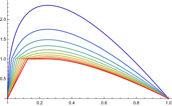
Figure 1: $0<a\leq\frac{1}{8}$

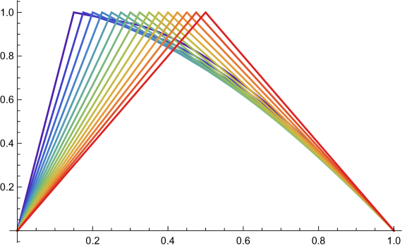
Figure 2: $\frac{1}{8}<a\leq\frac{1}{2}$

The directed geodesic has been studied recently, starting with the work in Dauvergne et al. (2018) showing the existence and uniqueness of this random continuous function for a given start and end point almost surely. Dauvergne et al. (2020) proved that the directed geodesic has $\frac{3}{2}$-variation, and Liu (2022b) found the scale of its fluctuations conditioned on the geodesic being unusually long. The recent work by Ganguly et al. (2023) shows that after rescaling, the long directed geodesic converges to a Brownian bridge. Liu (2022a) gives a formula for the joint distribution of the last passage geodesic passing through a point, its length before the point and its length after the point, but it is not clear how one can deduce asymptotic tail probabilities from this formula.

The special case when $a=\frac{1}{2}$ was solved in Agarwal and Basu (2024), and for this value of $a$ the geodesic made of two straight line is optimal (compare this to 1.2).

Let $\mathbb{R}_{\uparrow}^{4}$ denote pairs of elements of spacetime $(x,s,y,t)$ satisfying $s<t$. A directed metric (or metric) is a continuous function $e:\mathbb{R}_{\uparrow}^{4}\rightarrow\mathbb{R}$ satisfying the (reverse) triangle inequality

$$e(x,s,y,t)+e(y,t,z,u)\leq e(x,s,z,u)$$ (1.1)

The directed landscape $\mathcal{L}$ is a random directed metric that are defined by:

1. (Airy sheet marginals) For any $s<t$

   $$\mathcal{L}(x,s,y,t)\stackrel{{\scriptstyle d}}{{=}}\mathcal{S}(x(t-s)^{-\frac{2}{3}},y(t-s)^{-\frac{2}{3}})$$ (1.2)

   jointly in all $x,y$.

2. (Independent increments) For any disjoint set of time intervals $\{[s_{i},t_{i}]\}$, the random functions $\mathcal{L}(\cdot,s,\cdot,t)$ are independent.

3. (Metric composition law) For $r<s<t$ and for any $x,y$,

   $$\mathcal{L}(x,r,y,t)=\max_{z}(\mathcal{L}(x,r,z,s)+\mathcal{(}z,s,y,t))$$ (1.3)

Dauvergne (2024) showed that, almost surely, every pair of points is connected by one of 27 isomorphism types of geodesic networks.

Das, Dauvergne and Virág (2024) showed that every pair of points are connected by a unique rightmost geodesic. They study the rescaling

$$\mathcal{L}_{\varepsilon}(x,s,y,t)=\varepsilon\mathcal{L}(\varepsilon^{-\frac{1}{2}}x,s,\varepsilon^{-\frac{1}{2}}y,t)$$ (1.4)

They show the following Large deviation principle. For any open set $U$ and any closed set $V$ in the topology of uniform convergence on bounded sets,

$$\liminf_{\varepsilon\rightarrow 0}-\varepsilon^{\frac{3}{2}}\log{P(\mathcal{L}_{\varepsilon}\in U)}\leq\inf_{e\in U}I(e)$$ (1.5)

$$\limsup_{\varepsilon\rightarrow 0}-\varepsilon^{\frac{3}{2}}\log{P(\mathcal{L}_{\varepsilon}\in V)}\geq\inf_{e\in V}I(e)$$

where $I(e)$ is a lower semicontinuous function called the rate function. Moreover, $I$ is a “good rate function”, meaning that $I^{-1}[0,r]$ is compact for any $r\geq 0$, and has the following concrete description:

The Dirichlet metric $d$ is given by $d(x,s,y,t)=-\frac{(y-x)^{2}}{t-s}$. All finite rate metrics $e$ satisfy $e\geq d$, and arise from “planting measures” along countably many curves: For a curve $\gamma$ and a nonnegative measure density $\rho$, we can define

$$e_{\gamma,\rho}(\gamma(t_{1}),t_{1},\gamma(t_{2}),t_{2})=\int_{t_{1}}^{t_{2}}(\rho(t)-\gamma^{\prime}(t)^{2})dt$$ (1.6)

where $e_{\gamma,\rho}(x_{1},t_{1},x_{2},t_{2})=-\infty$ for any other choice of $x_{1},x_{2}$. Then the metric $e$ arising from planting measures along a finite or countable set of curves is the smallest metric which is bounded below by satisfying $e\geq d$, and for each curve $\gamma_{i}$ and planted measure $\rho_{i}$, $e\geq e_{\gamma_{i},\rho_{i}}$. All metrics not of this form have infinite rate.

For each such planted measure, the contribution to the rate function is $I_{i}=\frac{4}{3}\int\rho_{i}^{\frac{3}{2}}dt$, so that the rate function $I$ of a metric $e$ is the sum over all planted measures $I=\sum_{i}I_{i}$. Our goal in this paper is to find the lowest rate metric for which a geodesic $F$ from $(0,0)$ to $(0,1)$ passes through the point $(1,a)$.

Our metrics will generally have a measure planted along just one curve, which will be the geodesic from $(0,0)$ to $(0,1)$. Any measure planted outside of this geodesic will not increase its length, but may increase the length of paths other than $F$, which only reduces the possibility of $F$ being a geodesic, all while increasing the rate.

We can then define $e$ or $e(F,\rho)$ as the metric arising from planting $\rho$ along $F$, which will be our geodesic.

We will in fact prove a result about $e$: Suppose $\mathcal{M}_{\varepsilon}$ is a metric sampled from the conditional law of $\mathcal{L}_{\varepsilon}$, given that the rightmost geodesic $\gamma$ of $e$ from $(0,0)$ to $(0,1)$ satisfies $\gamma(a)\geq 1$.

Theorem 1.3.

As $\varepsilon\to 0$, $\mathcal{M}_{\varepsilon}\rightarrow e(F,\rho)$ in probability with respect to uniform convergence on bounded sets, with $F$ as in Theorem 1.2 and $\rho$ as given by:

$$\rho(t)=\begin{cases}\frac{1}{a^{2}(3-\sqrt{8a})^{2}},&\text{if }t\leq 2a\\ \frac{2}{at(3-\sqrt{8a})^{2}},&\text{if }2a\leq t\leq 1.\end{cases}$$

2 Solution of a relaxed problem

One possible candidate for $F$ is two straight line segments, from $(0,0)$ to $(1,a)$ and from $(1,a)$ to $(0,1)$, with $\rho$ just sufficient to compensate $d$, such that $e(0,0,F(t),t)=0,\forall t\in[0,1]$. However, for $a<\frac{1}{2}$, this will not be a geodesic: instead, there will be straight lines from $(0,0)$ to a point beyond $(1,a)$ whose Dirichlet length is greater than the length of $F$ to that point. As a result, the geodesic will skip the steeper line segment to $(1,a)$ and take such a straight line as a shortcut to $F$, and then follow part of the other line segment to $(0,1)$. Similarly, if $a>\frac{1}{2}$, it will follow part of the line segment from $(0,0)$ to $(1,a)$ and then shortcut the steep segment to proceed directly to $(0,1)$.

This suggests that we should try to solve for a metric where the segment from $(0,0)$ to $(1,a)$ is not skipped by such a shortcut. In other words, we should ask what is the lowest rate metric for which there is a geodesic candidate $F$, so that the distance from $(0,0)$ along $F$ to any point on $F$ is greater than the distance of a shortcut from $(0,0)$ to that point.

Inspired by this intuition, we will first solve an intermediate optimization problem: fix $F_{0}$ and $\rho_{0}$ (and therefore $e(F_{0},\rho_{0})$) for $t\in[0,t_{1}]$. Consider pairs $(F,\rho)$ that agree with $(F_{0},\rho_{0})$ on $[0,t_{1}]$. Which pair minimizes the rate of the metric $e=e(F,\rho)$ on the time interval $[t_{1},t_{2}]$, with the condition that the path along $F$ up to any $t\in[t_{1},t_{2}]$ is not worse than the shortcut from $(0,0)$ to $(F(t),t)$? In other words, what is the lowest rate metric $e=e(F,\rho)$ on $[t_{1},t_{2}]$ such that

$$d(0,0,F(t),t)\leq e(0,0,x_{1},t_{1})+e(x_{1},t_{1},F(t),t),\forall t\in(t_{1},t_{2})$$ (2.1)

In theory, the parameters of this optimization problem given by $e$ and $F$ up to time $t_{1}$. However, the only information used by the optimization problem are the scalar $e(0,0,x_{1},t_{1})$ and the starting point $x_{1}=F_{0}(t_{1}).$

We will store

$$b=e(F_{0},\rho_{0})(0,0,x_{1},t_{1})-d(0,0,x_{1},t_{1})=e(0,0,x_{1},t_{1})-\frac{x_{1}^{2}}{t_{1}}$$ (2.2)

as an initial condition in the form of the constant $b$ (where $b\geq 0$), so that we can focus on optimizing the path on $(t_{1},t_{2})$, and assume that $b$ is not so big as to cause (2.1) to hold for arbitrary $e\geq d$.

We will also assume that $\frac{x_{1}}{t_{1}}>\frac{x_{2}}{t_{2}}$. The problem is identical for $\frac{x_{1}}{t_{1}}<\frac{x_{2}}{t_{2}}$, but in this case, the entire picture should be flipped left to right.

We will define the function $F$, the rightmost geodesic candidate from $(x_{1},t_{1})$ to $(x_{2},t_{2})$, and $\rho$, the measure density planted along the path $(F(t),t)$, with respect to the Lebesgue measure on $t$. Since we are optimizing over $t\in[t_{1},t_{2}]$, we consider only the contribution to the rate function of the measure planted within this interval, $I_{2}$. Now we will formally state the relaxed optimization problem that we will solve.

Problem 2.1.

Given real numbers $t_{1},x_{1},t_{2},x_{2},b$ satisfying

• $0<t_{1}<t_{2}$

• $\frac{x_{1}}{t_{1}}>\frac{x_{2}}{t_{2}}$

• $0\leq b\leq\frac{(x_{2}-x_{1})^{2}}{t_{2}-t_{1}}+\frac{x_{1}^{2}}{t_{1}}-\frac{x_{2}^{2}}{t_{2}}$.

Minimize

$$I_{2}(F,\rho):=\frac{4}{3}\int_{t_{1}}^{t_{2}}\rho^{\frac{3}{2}}dt$$ (2.3)

over $F$, $\rho$ satisfying

• $F:[t_{1},t_{2}]\rightarrow\mathbb{R}$ is an absolutely continuous function, satisfying $F(t_{1})=x_{1}$, $F(t_{2})=x_{2}$.

• $\rho:[t_{1},t_{2}]\rightarrow\mathbb{R}$ is a nonnegative Lebesgue-measurable function.

• $g:[t_{1},t_{2}]\rightarrow\mathbb{R}$,

  $$g(t):=(b-\frac{F(t_{1})^{2}}{t_{1}})+\int_{t_{1}}^{t}(\rho(\tau)-F^{\prime}(\tau)^{2})d\tau+\frac{F(t)^{2}}{t}\geq 0,\forall t\in[t_{1},t_{2}].$$ (2.4)

We will call a pair $(F,\rho)$ feasible if it satisfies all of the above conditions (without necessarily minimizing $I_{2}$). The answer to this problem is given by the following proposition.

Proposition 2.2.

There exists a unique minimizing feasible pair $(F,\rho)$ for $I_{2}$, up to almost everywhere equivalence of $\rho$. Such a pair must satisfy the following conditions:

There exists $t_{B}\in[t_{1},t_{2}]$ such that $F$ is linear and $\rho$ is constant on $[t_{1},t_{B})$, and $F(t)=c_{1}\sqrt{t}+c_{2}t$ and $\rho(t)=(\frac{F(t)}{s}-F^{\prime}(t))^{2}$ for $t\in(t_{B},t_{2}]$, with $t_{B}=t_{1}$ if and only if $b=0$.

Moreover, $g^{\prime},F^{\prime},\rho$ are continuous at the merge point $t_{B}$.

The function $g$ keeps track of the difference in $\eqref{d=e+e}$. We can also rewrite (2.4) as

$$g(t)=b+\int_{t_{1}}^{t}(\rho(\tau)-(\frac{F(\tau)}{\tau}-F^{\prime}(\tau))^{2})d\tau$$ (2.5)

and so $g^{\prime}(t)=\rho(t)-(\frac{F(t)}{t}-F^{\prime}(t))^{2}$ almost everywhere.

The integral $\int_{t_{1}}^{t}\rho(\tau)d\tau$ is the contribution coming from the density $\rho$ planted along the curve. The remainder of the integral, $\int_{t_{1}}^{t}-F^{\prime}(\tau)^{2}d\tau$ is the Dirichlet metric term, penalizing $F$ for excessive curvature. The other terms, $\frac{F(t)^{2}}{t}-\frac{F(t_{1})^{2}}{t_{1}}=d(0,0,F(t),t)-d(0,0,F(t_{1}),t_{1})$, represent the difference in the Dirichlet metric of length of the shortcut to $t$, as compared to that to $t_{1}$.

Lastly, $b=g(t_{1})$ should be interpreted as the result of having previously optimized over $t<t_{1}$.

We may also write $g(F,\rho,b)$ instead of $g$ to emphasize which metric this $g$ arises from.

When it is not ambiguous, we may write $I_{2}$ instead of $I_{2}(F,\rho)$. Similarly, we will write $e$ for the associated metric $e(F,\rho)$.

We will prove Proposition 2.2 by establishing some basic facts about the minimizer, thereby reducing to two tractable optimization problems, one when $g$ is zero and one when $g$ is nonzero. We start with some generic lemmas about absolutely continuous functions.

Lemma 2.3.

Suppose $F$ is absolutely continuous on an interval $J\subset[t_{1},t_{2}]$. Then $\frac{F(t)}{t}$ is nonincreasing on $J$ if and only if $F^{\prime}(t)\leq\frac{F(t)}{t}$ for $t\in J$, and is constant on $J$ if and only if $F^{\prime}(t)=\frac{F(t)}{t}$ on $J$.

Proof.

$\frac{F(t)}{t}$ is absolutely continuous if and only if $F$ is, and

$$\frac{d}{dt}\frac{F(t)}{t}=\frac{1}{t}(F^{\prime}(t)-\frac{F(t)}{t}).$$ (2.6)

∎

Lemma 2.4.

Suppose $F(t)=\int_{a}^{t}f(\tau)d\tau$ is an absolutely continuous function on $[A,B]$, and $G(t)=max_{\tau\leq t}F(\tau)$. Then $G(t)=\int_{a}^{t}g(\tau)d\tau$, where $g=f\chi_{{}_{F=G}}$.

Proof.

If $V=\int|f|$ is the variation of $F$, define $H=V-G$. If $x<y$, clearly $G(x)\leq G(y)$. If $G(y)>G(x)$, suppose that $z\in(x,y]$ with $F(z)=G(y)$. Then

$$V(y)\geq V(x)+(F(z)-F(x))\geq V(x)+(G(y)-G(x)).$$ (2.7)

It follows that $H$ is nondecreasing, so $G=\int g$ and $H=\int h$ with $g+h=|f|$ and $g,h\geq 0$. When $F(t)\neq G(t)$, we have $g=0$ almost surely. When $F(t)=G(t)$, we must have $F^{\prime}(t)\geq 0$ (if $F^{\prime}$ exists), so almost surely either $f=0$ or $f>0$ and $F$ is locally increasing. In both cases, $h=0$ almost surely. Therefore, $g=|f|\chi_{{}_{F=G}}=f\chi_{{}_{F=G}}$. ∎

Lemma 2.5.

Suppose $G$ is absolutely continuous on $[A,B]$, and

$$\hat{F}(\tau)=\sup_{s<\tau<t}(\frac{t-\tau}{t-s}G(s)+\frac{\tau-s}{t-s}G(t))$$ (2.8)

is the concave majorant of $G$. Then $\int_{A}^{B}G^{\prime}(\tau)^{2}d\tau\geq\int_{A}^{B}\hat{F}(\tau)^{2}d\tau$.

Proof.

Recall that for a partition $P=\{a=\tau_{1},\tau_{2},\ldots,\tau_{n}=B\}$ of $[A,B]$, if

$$d_{F}(P)=\sum_{i=1}^{n-1}\frac{F(\tau_{i+1})^{2}-F(\tau_{i})^{2}}{\tau_{i+1}-\tau_{i}},$$ (2.9)

then the Dirichlet length of $F$ is $\sup_{P}{d_{F}(P)}$; see Lemma 5.1.6 in Dembo and Zeitouni (2009).

Suppose $P$ is a partition of $[A,B]$. For $2\leq i\leq n-1$, let $\hat{F}(\tau_{i})=\frac{t_{i}-\tau_{i}}{t_{i}-s_{i}}G(s_{i})+\frac{\tau-s_{i}}{t_{i}-s_{i}}G(t_{i})$, where $\hat{F}$ agrees with $G$ on $s_{i},t_{i}$ (if $\hat{F}(\tau_{i})=G(\tau_{i})$, set $s_{i}=t_{i}=\tau_{i}$). Let $P_{-}$ be the partition of $[t_{1},t]$ by including $s_{i}$ and $t_{i}$, and $P_{+}=P_{-}\cup P$. Since $P_{+}$ is a refinement of $P$, $d_{\hat{F}}(P)\leq d_{\hat{F}}(P_{+})$. Since $\hat{F}$ is a straight line between $s_{i}$, $\tau_{i}$ and $t_{i}$, $d_{\hat{F}}(P_{+})=d_{\hat{F}}(P_{-})$. Since $\hat{F}$ and $G$ agree on $P_{-}$, we have $d_{\hat{F}}(P_{-})=d_{G}(P_{-})$, so taking supremums we get that

$$\int_{t_{1}}^{t}G^{\prime}(\tau)^{2}d\tau\geq\int_{t_{1}}^{t}\hat{F}^{\prime}(\tau)^{2}d\tau.$$ (2.10)

∎

Lemma 2.6.

If $(F,\rho)$ is feasible, then there exists a feasible pair $(\hat{F},\rho)$ where $\hat{F}$ is concave and satisfies $\hat{F}^{\prime}(t)\leq\frac{\hat{F}(t)}{t}$ for all $t\in[t_{1},t_{2}]$. In particular, $I_{2}(F,\rho)=I_{2}(\hat{F},\rho)$. Moreover, if $F\neq\hat{F}$, then $g(F,\rho,b)(t_{2})<g(\hat{F},\rho,b)(t_{2})$.

Proof.

Note that $F(t)$ is absolutely continuous if and only if $\frac{F(t)}{t}$ is. Define $\frac{G(t)}{t}=\min_{\tau\leq t}\frac{F(\tau)}{\tau}$. Then by Lemma 2.4, $\frac{G(t)}{t}$ is absolutely continuous and is the integral of $(\frac{F(t)}{t})^{\prime}\chi_{{}_{A}}$, where $A=\{t:\frac{F(t)}{t}=\frac{G(t)}{t}\}$. It follows that $G$ is absolutely continuous and its derivative is almost everywhere equal to $F^{\prime}(t)$ on $A$ and to $\frac{G(t)}{t}$ on $[t_{1},t_{2}]\backslash A$.

In both cases, $(\frac{G(t)}{t}-G^{\prime}(t))^{2}\leq(\frac{F(t)}{t}-F^{\prime}(t))^{2}$, so for $t\in[t_{1},t_{2}]$, we have

$$g(G,\rho,b)(t)=\int_{t_{1}}^{t}\rho-(\frac{G(t)}{t}-G^{\prime}(t))^{2}\geq\int_{t_{1}}^{t}\rho-(\frac{F(t)}{t}-F^{\prime}(t))^{2}=g(F,\rho,b),$$ (2.11)

with equality at $t=t_{2}$ if and only if $G^{\prime}=F^{\prime}$ almost everywhere, i.e. if and only if $G=F$.

Next, we will define $\hat{F}$ as the concave majorant of $G$, by

$$\hat{F}(\tau)=\sup_{s<\tau<t}(\frac{t-\tau}{t-s}G(s)+\frac{\tau-s}{t-s}G(t)).$$ (2.12)

Note that either this supremum is attained or $\hat{F}(\tau)=G(\tau)$. Since $G$ was continuous, $\hat{F}$ is also continuous.

Since it is concave, $\hat{F}$ is absolutely continuous. We will show that $\hat{F}$ inherits from $G$ the property that $\frac{\hat{F}(\tau)}{\tau}\geq\hat{F}^{\prime}(\tau)$. When $\hat{F}\neq G$, we have $\hat{F}(\tau)=\frac{t-\tau}{t-s}G(s)+\frac{\tau-s}{t-s}G(t)$ and $\hat{F}^{\prime}(\tau)=\frac{G(t)-G(s)}{t-s}$. By definition of $G$, $\frac{G(t)}{t}\leq\frac{G(s)}{s}$, so

$$\hat{F}^{\prime}(\tau)=\frac{G(t)-G(s)}{t-s}\leq\frac{G(t)}{t}\leq\frac{G(s)}{s}.$$ (2.13)

since $\frac{G(t)}{t}$ is the mediant of the other two fractions. Then by (2.13) twice,

$$\frac{\hat{F}(\tau)}{\tau}=\frac{1}{\tau}(\frac{t-\tau}{t-s}G(s)+\frac{\tau-s}{t-s}G(t))\geq\frac{\hat{F}^{\prime}(\tau)}{\tau(t-s)}((t-\tau)s+(\tau-s)t)=\hat{F}^{\prime}(\tau).$$ (2.14)

Next, If $\tau$ is a limit point of the set where $\hat{F}\neq G$, then with countably many exceptions at the jump discontinuities of $\hat{F}^{\prime}$, we can infer the same inequality by taking limits. Otherwise, $\hat{F}$ is equal to $G$ in a neighborhood of $\tau$, so $\hat{F}^{\prime}(\tau)=G^{\prime}(\tau)\leq\frac{G(t)}{t}=\frac{\hat{F}(t)}{t}$.

To see that $\hat{F}$ is feasible, we will compare $g(\hat{F},\rho,b)$ and $g(G,\rho,b)$. First consider $t\in[t_{1},t_{2}]$ with $\hat{F}(t)=G(t)$. By Lemma 2.5,

$$\int_{t_{1}}^{t}-\hat{F}^{\prime}(\tau)^{2}d\tau\geq\int_{t_{1}}^{t}-G^{\prime}(\tau)^{2}d\tau.$$ (2.15)

Thus $g(\hat{F},\rho,b)(t)\geq g(G,\rho,b)(t)$, with equality if and only if $G$ is linear on every interval where $\hat{F}$ is linear, i.e. if $\hat{F}$ coincides with $G$ on $[t_{1},t]$. In particular, if $\hat{F}\neq G$, then $g(\hat{F},\rho,b)(t_{2})>g(G,\rho,b)(t_{2})$.

Now let $\tau\in[t_{1},t_{2}]$ with $\hat{F}(\tau)\neq G(\tau)$, so that $\hat{F}(\tau)=\frac{t-\tau}{t-s}G(s)+\frac{\tau-s}{t-s}G(t)$. Let $\hat{G}$ be equal to $G$ except on $[s,\tau]$, where it is replaced by a straight line from $(G(s),s)$ to $(G(\tau),\tau)$. Then clearly $g(\hat{G},\rho,b)(\tau)\geq g(G,\rho,b)(\tau)$. Observe that for a linear function $L$, the integral $\int_{s}^{\tau}-(\frac{L(t^{\prime})}{t^{\prime}}-L^{\prime}(t^{\prime}))^{2}$ in (2.5) is a function of $L(s)$ and $L^{\prime}$, quadratic in $L^{\prime}$, and maximized at $L^{\prime}(s)=\frac{L(s)}{s}$. Then since $\hat{G}^{\prime}\leq\hat{F}^{\prime}\leq\frac{F(s)}{s}$, we have $g(\hat{F},\rho,b)(\tau)\geq g(\hat{G},\rho,b)(\tau)$.

As a result, $(\hat{F},\rho)$ is feasible, and $\hat{F}$ is concave with $\hat{F}^{\prime}(t)\leq\frac{\hat{F}(t)}{t}$ for all $t\in[t_{1},t_{2}]$.

When $F\neq\hat{F}$, either $G\neq F$ or $\hat{F}\neq G$, and in both cases we have shown that $g(F,\rho,b)(t_{2})<g(\hat{F},\rho,b)(t_{2})$.

Lastly, $I(F,\rho)=I(\hat{F},\rho)$, since $I$ depends only on $\rho$.

∎

With the added control on $F$, the set of geodesics becomes compact, if their rate does not diverge to infinity:

Lemma 2.7.

Suppose $F_{i}$ are concave and satisfy $F_{i}^{\prime}(t)\leq\frac{F_{i}(t)}{t}$ as in Lemma 2.6, with $F_{i}(t_{1})=x_{1}$ and $F_{i}(t_{2})=x_{2}$. Then some subsequence of the $F_{i}$ converges uniformly to a concave function $F$ on any interval $[t_{1},t_{2}^{\prime}],t_{2}^{\prime}<t_{2}$, with $F^{\prime}(t)\leq\frac{F^{\prime}(t)}{t}$, as well as $F(t_{1})=x_{1}$.

Proof.

Note that $F_{i}(t)\in[\frac{t_{2}-t}{t_{2}-t_{1}}x_{1}+\frac{t-t_{1}}{t_{2}-t_{1}}x_{2},t\frac{x_{1}}{t_{1}}]$, so by enumerating the rationals and repeatedly taking subsequence, we may assume that $F_{i}(q)$ converge to some $F(q)$ for every rational $q$.

When restricted to $\mathbb{Q}$, $F$ must be concave as it is a limit of concave functions, and therefore can be extended continuously in its interior. It is also continuous at $t_{1}$ since $F_{i}^{\prime}(t_{1})$ is bounded above.

Since $G_{i}(t):=t\frac{x_{1}}{t_{1}}-F_{i}(t)$ are nondecreasing functions, $G_{i}(r)$ must converge to $G(r)$ for any $r\in[t_{1},t_{2})$, where $G(r)=r\frac{x_{1}}{t_{1}}-F(r)$. On an interval $[t_{1},t_{2}^{\prime}]$, for $t_{2}^{\prime}<t_{2}$, we can consider convergence at the partition points

$$G^{-1}(G(t_{1})+2^{-n}k(G(t_{2}^{\prime})-G(t_{1})),k\in[0,2^{n}]\cap\mathbb{Z},$$ (2.16)

to show that $G_{i}$ is eventually within $2^{-n}+\varepsilon$ of $G$ on $[t_{1},t_{2}^{\prime}]$. Thus $G_{i}\rightarrow G$ and hence $F_{i}\rightarrow F$ uniformly on intervals bounded away from $t_{2}$.

The conditions on $F$ are all inherited from those on $F_{i}$. ∎

We introduce some more intermediate lemmas to prove the existence of a minimizing pair $(F,\rho)$.

Lemma 2.8.

Suppose $(F,\rho)$ is feasible. Then there is a nonincreasing $\hat{\rho}$ with $(F,\hat{\rho})$ feasible, and $I_{2}(F,\hat{\rho})=I_{2}(F,\rho)$. Moreover, $\hat{\rho}$ has the same distribution as $\rho$, in the sense that $\lambda(\rho^{-1}([A,\infty)))=\lambda(\hat{\rho}^{-1}([A,\infty))),\forall A\geq 0$, and satisfies $\int_{t_{1}}^{t}\hat{\rho}(\tau)d\tau\geq\int_{t_{1}}^{t}\rho(\tau)d\tau$ for any $t\in[t_{1},t_{2}]$. Here $\lambda$ denotes the Lebesgue measure.

Proof.

We define $\hat{\rho}$ to be the nonincreasing sorted version of $\rho$. In other words, for $\rho:[t_{1},t_{2}]\rightarrow\mathbb{R}^{+}$, define

$$\nu(A)=\lambda(\rho^{-1}([A,\infty)))$$ (2.17)

$$\hat{\rho}(t)=\inf_{\nu(A)\geq t-t_{1}}A$$ (2.18)

It is easy to see that $\hat{\rho}$ is nonincreasing and has the same distribution as $\rho$.

Then for any $t\in[t_{1},t_{2}]$, we have

$$\int_{t_{1}}^{t}\rho(\tau)d\tau=\int_{0}^{\infty}\lambda(\rho^{-1}([A,\infty))\cap[t_{1},t])dA.$$ (2.19)

Since $\lambda(\rho^{-1}([A,\infty))\cap[t_{1},t])\leq\min(\lambda(\rho^{-1}([A,\infty)),\lambda([t_{1},t]))$, and since the latter term is just $\lambda(\hat{\rho}^{-1}([A,\infty))\cap[t_{1},t])$, the integral in (2.19) is bounded above by

$$\int_{0}^{\infty}\lambda(\hat{\rho}^{-1}([A,\infty))\cap[t_{1},t])dA=\int_{t_{1}}^{t}\hat{\rho}(\tau)d\tau.$$ (2.20)

Then

$$g(F,\hat{\rho},b)(t)-g(F,\rho,b)(t)=\int_{t_{1}}^{t}(\hat{\rho}-\rho)\geq 0,$$ (2.21)

so $g(F,\hat{\rho},b)\geq g(F,\rho,b)\geq 0$, and $I_{2}(F,\rho)=\frac{4}{3}\int\rho^{\frac{3}{2}}=I_{2}(F,\hat{\rho})$.

∎

Lemma 2.9.

Suppose $F_{i}:[A,B]\rightarrow\mathbb{R}$ are absolutely continuous functions with $\int_{A}^{B}F_{i}^{2}<\infty$, converging uniformly to $F$. Then

$$\int_{A}^{B}F^{\prime 2}\leq\liminf_{n}\int_{A}^{B}F_{n}^{\prime 2}.$$ (2.22)

Proof.

The Dirichlet norm of $F$, $\int_{A}^{B}F^{2}$, is also given by the supremum over partitions $P$ of $[A,B]$ with breaks at $a=t_{0},t_{1},\ldots,t_{n}=B$ of $d_{P}(F)$, where

$$d_{P}(F)=\sum_{i=1}^{n}\frac{(F(t_{i})-F(t_{i-1}))^{2}}{t_{i}-t_{i-1}}.$$ (2.23)

For any given $P$, we can choose $N$ such that $||F-F_{n}||_{u}$ is sufficiently small for $n>N$, and then $d_{P}(F_{n})$ can be made arbitrarily close to $d_{P}(F)$. Since $\liminf_{n}\int_{A}^{B}F_{n}^{2}\geq\liminf_{n}d_{P}(F_{n})$, we have $d_{P}(F)\leq\liminf_{n}\int_{A}^{B}F_{n}^{2}$, so the result follows by taking the supremum over all partitions $P$. ∎

Lemma 2.10.

If $\{\rho_{i}\}_{i=1}^{\infty}$ is a sequence of nonincreasing, nonnegative functions on $[A,B]$ with $\int_{A}^{B}\rho_{i}^{\frac{3}{2}}<M$, then it admits a subsequence that converges in $L^{1}$ to some $\rho$, with $\int_{A}^{B}\rho^{\frac{3}{2}}\leq\liminf\int_{A}^{B}\rho_{i}^{\frac{3}{2}}$.

Proof.

Note that $\int_{A}^{B}\rho_{i}^{\frac{3}{2}}<M$ implies that $\int_{A}^{B}\rho_{i}<L:=(B-A)^{\frac{1}{3}}M^{\frac{2}{3}}$ by Holder’s inequality. For $\varepsilon>0$, we must have $\rho_{i}(A+\varepsilon)<\frac{L}{\varepsilon}$. Then on the interval $[A+\varepsilon,B]$, we have $\rho_{i}(t)=\rho_{i}(A+\varepsilon)-\mu_{i}([A+\varepsilon,t])$ for some positive, uniformly bounded measures $\mu_{i}$. By passing to a subsequence, we may assume that $\rho_{i}(A+\varepsilon)$ converge and that $\mu_{i}$ converge weakly. Then

$$\int_{A+\varepsilon}^{B}|\rho(t)-\rho_{i}(t)| \leq(B-A)(\rho(A+\varepsilon)-\rho_{i}(A+\varepsilon))$$ (2.24)

$$+\int_{A+\varepsilon}^{B}|\mu([A+\varepsilon,t])-\mu_{i}([A+\varepsilon,t])|dt$$

The first term converges to zero, and the integral term is, by Fubini’s theorem, equal to

$$\int_{A+\varepsilon}^{B}\int_{A+\varepsilon}^{t}1d(\mu-\mu_{i})(\tau)dt=\int_{A+\varepsilon}^{B}(B-\tau)d(\mu-\mu_{i})(\tau).$$ (2.25)

This goes to zero since $\mu_{i}\rightarrow\mu$, so $\rho_{i}$ converge to $\rho$ in $L^{1}$ on $(A+\varepsilon,B]$.

By Holder’s inequality, $\int_{A}^{A+\varepsilon}\rho(\tau)d\tau\leq\varepsilon^{\frac{1}{3}}M^{\frac{2}{3}}$, so $\rho_{i}\rightarrow\rho$ in $L^{1}$ on $[A,B]$. Since the unit ball of $L^{q}([A,B])$ is closed in $L^{p}([A,B])$ for $p<q$, we have $\int_{A}^{B}\rho^{\frac{3}{2}}(\tau)d\tau\leq\liminf\int_{A}^{B}\rho_{i}^{\frac{3}{2}}(\tau)d\tau$. ∎

Lemma 2.11.

There exists a feasible pair $(F,\rho)$ with $I_{2}(F,\rho)=\inf_{\hat{F},\hat{\rho}}I_{2}(\hat{F},\hat{\rho})$, where the infimum is taken over all feasible $(\hat{F},\hat{\rho})$.

Proof.

Observe that the set of feasible $(\hat{F},\hat{\rho})$ is nonempty: if $\hat{F}$ is the straight line connecting $(x_{1},t_{1})$ to $(x_{2},t_{2})$, and $\hat{\rho}=\frac{x_{1}^{2}}{t_{1}^{2}}+\frac{x_{2}^{2}}{t_{2}^{2}}$ on $[t_{1},t_{2}]$, then $(\hat{F},\hat{\rho})$ is feasible. By Lemma 2.6, there exist feasible pairs $(F_{i},\rho_{i})_{i=1}^{\infty}$ with $F_{i}$ concave and $F_{i}^{\prime}(t)\leq\frac{F_{i}(t)}{t}\forall t\in[t_{1},t_{2}]$, such that $\lim_{i\rightarrow\infty}I_{2}(F_{i},\rho_{i})=\inf_{\hat{F},\hat{\rho}}I_{2}(\hat{F},\hat{\rho})$. By Lemma 2.8, we may also assume that each $\rho_{i}$ is nonincreasing. We will find a converging subsequence whose rate will therefore be minimal.

Let $M=\max_{i}I_{2}(F_{i},\rho_{i})$, so that $\int_{t_{1}}^{t_{2}}\rho_{i}(\tau)^{\frac{3}{2}}d\tau\leq\frac{3}{4}M$. Then $\int_{t_{1}}^{t_{2}}\rho(\tau)d\tau\leq(t_{2}-t_{1})^{\frac{1}{3}}(\frac{3}{4}M)^{\frac{2}{3}}$ by Holder’s inequality. Then for $D:=(t_{2}-t_{1})^{\frac{1}{3}}(\frac{3}{4}M)^{\frac{2}{3}}+b$, we must have $\int_{t_{1}}^{t_{2}}F_{i}^{\prime}(\tau)^{2}d\tau\leq D$.

By Lemma 2.7, by passing to a subsequence we may assume that $F_{i}\rightarrow F$ uniformly on sets bounded away from $t_{2}$. Moreover, for $\varepsilon>0$, if $\delta=\frac{\varepsilon^{2}}{D}$, we must have $|F_{i}(t)-x_{2}|\leq\varepsilon$ whenever $|t-t_{2}|\leq\delta$. Thus $F_{i}$ converge uniformly to $F$.

Similarly, by Lemma 2.10, by passing to a subsequence again we may assume that $\rho_{i}\rightarrow\rho$ in $L^{1}$ and that $\int\rho^{\frac{3}{2}}=\frac{3}{4}\inf_{\hat{F},\hat{\rho}}I_{2}(\hat{F},\hat{\rho})$.

It follows by Lemma 2.9 that $g(F,\rho,b)(t)\geq\limsup g(F_{i},\rho_{i},b)(t)\geq 0$, so $(F,\rho)$ is feasible, and moreover that

$$I_{2}(F,\rho)=\frac{4}{3}\int_{t_{1}}^{t_{2}}\rho^{\frac{3}{2}}(\tau)d\tau=\lim_{i\rightarrow\infty}\frac{4}{3}\int_{t_{1}}^{t_{2}}\rho_{i}^{\frac{3}{2}}(\tau)d\tau=\inf_{\hat{F},\hat{\rho}}I_{2}(\hat{F},\hat{\rho}).$$ (2.26)

∎

Lemma 2.12.

Suppose $(F,\rho)$ is feasible and minimizes $I_{2}$. Then $g(F,\rho,b)(t_{2})=0$. In particular, $F$ is concave and $F^{\prime}(t)\leq\frac{F(t)}{t}$ for all $t\in[t_{1},t_{2}]$.

Proof.

Since $b\leq\frac{(x_{2}-x_{1})^{2}}{t_{2}-t_{1}}+\frac{x_{1}^{2}}{t_{1}}-\frac{x_{2}^{2}}{t_{2}}$, if $\rho$ is zero almost everywhere, then $b=\frac{(x_{2}-x_{1})^{2}}{t_{2}-t_{1}}+\frac{x_{1}^{2}}{t_{1}}-\frac{x_{2}^{2}}{t_{2}}$ and $F$ is linear on $[t_{1},t_{2}]$ and we compute $g(t_{2})=0$. Otherwise, $\int\rho>0$, and suppose for the sake of contradiction that $g(t_{2})>0$. The integral $\int_{t}^{t_{2}}\rho(\tau)d\tau$ is a continuous function of $t$ decreasing to zero, so fix $t$ sufficiently close to $t_{2}$ so that $0<\int_{t}^{t_{2}}\rho(\tau)d\tau<g(t_{2})$. From (2.5), since $g^{\prime}(\tau)\leq\rho(\tau)$, we will show that $(F,\hat{\rho}:=\chi_{{}_{[t_{1},t]}}\rho)$ is feasible: if $\hat{g}=g(F,\hat{\rho},b)$, then we have $\hat{g}(t^{\prime})=g(t^{\prime})$ for $t^{\prime}\leq t$, and for $t^{\prime}\in[t,t_{2}]$,

$$\hat{g}(t^{\prime})\geq\hat{g}(t_{2})=g(t_{2})-\int_{t}^{t_{2}}\rho(\tau)d\tau>0,$$ (2.27)

so $(F,\hat{\rho})$ is feasible. But then $I_{2}(F,\hat{\rho})<I_{2}(F,\rho)$, contradicting minimality of $I_{2}(F,\rho)$.

If $F$ is not of the stated form, then by Lemma 2.6 there exists $\hat{F}$ with $(\hat{F},\rho)$ also minimizing $I_{2}$ such that $g(\hat{F},\rho,b)(t_{2})>g(F,\rho,b)(t_{2})\geq 0$, which is a contradiction.

∎

From this point forth, we will assume that $(F,\rho)$ is a feasible pair minimizing $I_{2}$ and satisfying the conclusion of Lemma 2.6, and that $g$ is the function arising from the definition in $\eqref{defineg}$. We will also assume by Lemma 2.8 that $\rho$ is nonincreasing.

Lemma 2.13.

Suppose for some interval $(p,q)\subset(t_{1},t_{2})$, $g(t)>0,\forall t\in(p,q)$. Then $F$ is linear and $\rho$ is constant on $(p,q)$.

Proof.

Fix $t\in(p,q)$. Pick $\varepsilon<\min(\frac{t_{2}-t}{2},\frac{g(t)}{4}(\frac{\max F}{t_{1}}-\min_{t^{\prime}<\frac{t+t_{2}}{2}}F^{\prime}(t^{\prime}))^{-2})$, sufficiently small so that $\int_{t-\varepsilon}^{t}\rho(\tau)d\tau<\frac{g(t)}{2}$. Suppose $F$ is not linear on $[t-\varepsilon,t+\varepsilon]$. Let $G=F$ outside of $(t-\varepsilon,t+\varepsilon)$, and define $G$ linearly on $[t-\varepsilon,t+\varepsilon]$. For $t\in(t-\varepsilon,t+\varepsilon)$, we have

$$g(G,\rho,b)(t^{\prime})\geq g(F,\rho,b)(t^{\prime})-\int_{t-\varepsilon}^{t^{\prime}}(\frac{G(\tau)}{\tau}-G^{\prime}(\tau))^{2}d\tau$$ (2.28)

Observe that $\frac{G(\tau)}{\tau}\geq G^{\prime}(\tau)$ on $(t-\varepsilon,t+\varepsilon)$: $G^{\prime}(\tau)$ is constant, so we just need to show that $G$ does not cross the parallel line $x=\tau G^{\prime}$ on this interval. But by Lemma 2.6,

$$G(t-\varepsilon)=F(t-\varepsilon)\geq(t-\varepsilon)F^{\prime}(t-\varepsilon)\geq(t-\varepsilon)G^{\prime}.$$ (2.29)

Next, since $(-\frac{F(t)}{t}-F^{\prime}(t))^{2}\leq g^{\prime}(t)\leq\rho(t)$ by (2.5), equation (2.28) is bounded below by

$$g(F,\rho,b)(t)-\int_{t-\varepsilon}^{t}\rho(\tau)d\tau-\int_{t-\varepsilon}^{t+\varepsilon}(\frac{G(\tau)}{\tau}-G^{\prime}(\tau))^{2}d\tau>g(t)-\frac{g(t)}{2}-\frac{g(t)}{2}=0,$$ (2.30)

where the inequality on the second integral comes from taking an upper and lower bound on $G$ and $G^{\prime}$, as in the choice of $\varepsilon$. By choice of $\varepsilon$, we have $g(G,\rho,b)(t^{\prime})>0$ for $t^{\prime}\in(t-\varepsilon,t+\varepsilon)$, and since the straight line has the shortest Dirichlet length, $g(G,\rho,b)(t^{\prime})>g(F,\rho,b)(t^{\prime})$ for $t^{\prime}>t+\varepsilon$. But then $(G,\rho)$ is feasible and minimizes $I_{2}$, while $g(G,\rho,b)(t_{2})>0$, in contradiction to Lemma 2.12.

Now suppose $\rho$ is not constant on $[t-\varepsilon,t+\varepsilon]$, and let $\lambda$ be the average value of $\rho$ on the interval. If, for $\delta\in(0,1)$, we define $\rho_{\delta}$ equal to $(1-\delta)\rho+\delta\lambda$ on $[t-\varepsilon,t+\varepsilon]$ and equal to $\rho$ otherwise, then $I_{2}(F,\rho_{\delta})<I_{2}(F,\rho)$ due to convexity of $x\mapsto x^{\frac{3}{2}}$. But $g(F,\rho,b)=g(F,\rho_{\delta},b)$ outside of the interval, and for sufficiently small $\delta$, $g(F,\rho_{\delta},b)>0$ is positive on the interval $[t-\varepsilon,t+\varepsilon]$ as well, contradicting minimality of $(F,\rho)$.

Thus, there is some neighborhood of $t$ on which $F$ is linear and $\rho$ is constant.

Considering various $t\in(p,q)$, these neighborhoods make an open cover of $[p+\varepsilon,q-\varepsilon]$, which has a finite subcover. Since line segments on overlapping open sets must have the same slope, $F$ is linear on $(p,q)$. Similarly, $\rho$ is constant on $(p,q)$. ∎

Lemma 2.14.

If $g=0$ on the interval $[s_{1},s_{2}]$, then $F^{\prime}$ and $\rho$ are absolutely continuous on these intervals.

Proof.

For $s\in[s_{1},s_{2}]$, we have $g^{\prime}(s)=0$, so, almost surely

$$\rho(s)-(\frac{F(s)}{s}-F^{\prime}(s))^{2}=0.$$ (2.31)

$\rho$ is nonincreasing, so it is either continuous or has downward jump discontinuities. Similarly, $F^{\prime}$ is nonincreasing, so $\frac{F(s)}{s}-F^{\prime}(s)$ has only upward jump discontinuities. Since $F^{\prime}(t)\leq\frac{F(t)}{t}$ by Lemma 2.6, $(\frac{F(s)}{s}-F^{\prime}(s))^{2}$ has only upward jump discontinuities. Then the left side of (2.31) can have only downward jump discontinuities. But the right side of (2.31) is equal to the constant zero, so $\rho$ and $F^{\prime}$ cannot have any discontinuities.

Next, (2.31) can be rewritten as

$$\frac{F(s)}{s}=\sqrt{\rho(s)}+F^{\prime}(s).$$ (2.32)

Since $\rho$ and $F^{\prime}$ are continuous and nondecreasing, we can define nonnegative measures $\mu_{1}$ and $\mu_{2}$ by

$$\sqrt{\rho(s)}=\sqrt{\rho(s_{1})}+\mu_{1}([s_{1},s]),F^{\prime}(s)=F^{\prime}(s_{1})+\mu_{2}([s_{1},s]).$$ (2.33)

But since $\frac{F(s)}{s}$ is absolutely continuous, by (2.32), $\mu_{1}+\mu_{2}$ is continuous with respect to the lebesgue measure and hence $\mu_{1},\mu_{2}<<\lambda$. Thus $F^{\prime}$ and $\sqrt{\rho}$ are absolutely continuous, and therefore so is $\rho$.

∎

Lemma 2.15.

If $g(t)=0$ for $t\in[s_{1},s_{2}]$, then on this interval, $F(t)=c_{1}\sqrt{t}+c_{2}t$, and $\rho(t)=(\frac{F(t)}{t}-F^{\prime}(t))^{2}$.

The Euler-Lagrange equation from calculus of variations states that the function $f=\rho^{\frac{3}{2}}$ must satisfy the equation

$$\frac{\partial f}{\partial F}=\frac{d}{dt}\frac{\partial f}{\partial F^{\prime}}.$$ (2.34)

We give a quick alternative way to see this through calculus.

Proof.

The equality $\rho(t)=(\frac{F(t)}{t}-F^{\prime}(t))^{2}$ follows directly from the definition of $g$. Let $\phi$ be a nonnegative smooth function supported on $[s_{1},s_{2}]$, and define

$$F_{\alpha}=F+\alpha\phi,\rho_{\alpha}(t)=(\frac{F_{\alpha}(t)}{t}-F_{\alpha}^{\prime}(t))^{2}.$$ (2.35)

Now consider the effect of $\alpha$ on $I_{2}=\int\rho^{\frac{3}{2}}=\int(\frac{F(s)}{s}-F^{\prime})^{3}$:

$$\frac{d}{d\alpha}(\frac{3}{4}I_{2}(F_{\alpha},\rho_{\alpha}))\Bigr{|}_{\alpha=0} =\frac{d}{d\alpha}\int_{s_{1}}^{s_{2}}(\frac{F_{\alpha}(s)}{s}-F_{\alpha}^{\prime}(s))^{3}ds$$ (2.36)

$$=\int_{s_{1}}^{s_{2}}\frac{\partial F_{\alpha}(s)}{\partial\alpha}\frac{\partial}{\partial F(s)}(\frac{F(s)}{s}-F^{\prime}(s))^{3}ds$$

$$+\int_{s_{1}}^{s_{2}}\frac{\partial F_{\alpha}^{\prime}(s)}{\partial\alpha}\frac{\partial}{\partial F^{\prime}(s)}(\frac{F(s)}{s}-F^{\prime}(s))^{3}ds$$

Using the linear dependence of $F_{\alpha}$ on $\alpha$, we see this is equal to

$$\int_{s_{1}}^{s_{2}}(\phi(s-t))3(\frac{F(s)}{s}-F^{\prime}(s))^{2}(\frac{1}{s})ds$$ (2.37)

$$+ \int_{s_{1}}^{s_{2}}(\phi^{\prime}(s-t))3(\frac{F(s)}{s}-F^{\prime}(s))^{2}(-1)ds$$

This derivative must be equal to zero for $F=F_{0}$ and for any $\phi$, as otherwise $I_{2}$ will be lower for $F_{\alpha}$ for some $\alpha$ sufficiently close to zero. Since $\phi$ was arbitrary, this means that $3(\frac{F(s)}{s}-F^{\prime}(s))^{2}(\frac{1}{s})$ is the weak derivative of $3(\frac{F(s)}{s}-F^{\prime}(s))^{2}(-1)$. Since the latter is absolutely continuous by Lemma 2.14, we can infer the differential equation

$$-\frac{d}{ds}(\frac{F(s)}{s}-F^{\prime}(s))^{2}=\frac{1}{s}(\frac{F(s)}{s}-F^{\prime}(s))^{2}.$$ (2.38)

This simplifies to

$$-(\frac{F^{\prime}(s)}{s}-\frac{F(s)}{s^{2}}-2F^{\prime\prime}(s))(\frac{F(s)}{s}-F^{\prime}(s))=0.$$ (2.39)

Now suppose $F^{\prime}(t)=\frac{F(t)}{t}$ for some $t\in(s_{1},s_{2})$. Since $\rho$ is nonincreasing by Lemma 2.8, this implies that $\rho=0$ on $[t,s_{2}]$, so $F^{\prime}(s_{2})=\frac{F(s_{2})}{s_{2}}$. By Lemma 2.6, $F$ is concave, so $F(t_{1})\leq F(s_{2})-\frac{F(s_{2})}{s_{2}}s_{2}(s_{2}-t_{1})$, and therefore $F(s_{2})\geq x_{1}\frac{s_{2}}{t_{1}}$. But by Lemma 2.3, $\frac{F(s_{2})}{s_{2}}$ is nonincreasing, so $F^{\prime}(s)=\frac{F(s)}{s}=\frac{x_{1}}{t_{1}}$ must hold for any $s\in[t_{1},s_{2}]$. Thus $F$ is linear on $[s_{1},s_{2}]$, which satisfies the conclusion of this lemma with $c_{1}=0$.

Otherwise, we can divide (2.39) by $-(\frac{F(s)}{s}-F^{\prime}(s))$, and we get the following differential equation:

$$-\frac{F(t)}{t^{2}}+\frac{F^{\prime}(t)}{t}-2F^{\prime\prime}(t)=0.$$ (2.40)

Since we know the antiderivative, $(\frac{F(t)}{t}-2F^{\prime}(t))$, is absolutely continuous, it must be equal to some constant $C_{1}$. We can then divide by $\sqrt{t}$ to get

$$\frac{F(t)}{t^{\frac{3}{2}}}-2\frac{F^{\prime}(t)}{\sqrt{t}}=\frac{C_{1}}{\sqrt{t}}.$$ (2.41)

Again the antiderivative of the left side, $-\frac{2F(t)}{\sqrt{t}}$, is absolutely continuous, and so integrating again yields

$$F(t)=-C_{1}\sqrt{t}-2C_{2}t.$$ (2.42)

∎

Lemma 2.16.

There exists $t_{B}\in[t_{1},t_{2}]$ such that $g(t)=0$ for $t\in[t_{B},t_{2}]$, and $g(t)>0$ for $t\in[t_{1},t_{B})$. $t_{B}=t_{1}$ if and only if $b=0$.

Proof.

We have $g(t_{2})=0$ by Lemma 2.12. Suppose the claim is false; then there exists some $s\in[t_{1},t_{2}]$ such that $g(s)>0$, but $g$ has a zero both above and below $s$. Let $p$ be the greatest zero below $s$ and $q$ be the least zero above $s$, so that $g(t)>0$ for $t\in(p,q)$, and $g(p)=g(q)=0$. By Lemma 2.13, $\rho$ is constant and $F$ is linear on $(p,q)$, so $F^{\prime}(t)$ is also constant. By Lemma 2.3, $\frac{F(t)}{t}$ is nonincreasing, so this means that $g^{\prime}(t)=\rho(t)-(\frac{F(t)}{t}-F^{\prime}(t))^{2}$ is nondecreasing, which is impossible as $g(p)=0$, $g(s)>0$, $g(q)=0$. $t_{B}$ is the smallest $t$ such that $g(t)=0$, so $t_{B}=t_{1}$ if and only if $g(t_{1})=b=0$. ∎

Proof of Proposition 2.2.

By Lemma 2.11, there exists a minimizing feasible pair for $I_{2}$. Suppose $(F_{1},\rho_{1})$ and $(F_{2},\rho_{2})$ are both minimizers. Since $g$ is concave as a function of $F$ and linear in $\rho$, it must be that $(\frac{1}{2}(F_{1}+F_{2}),\frac{1}{2}(\rho_{1}+\rho_{2}))$ is feasible. Since $\int\rho^{\frac{3}{2}}$ is strictly convex, it follows that $I_{2}(\frac{1}{2}(F_{1}+F_{2}),\frac{1}{2}(\rho_{1}+\rho_{2}))\leq I_{2}(F_{1},\rho_{1})$, with equality possible only when $\rho_{1}=\rho_{2}$ almost everywhere. Therefore, the optimal $\rho$ is unique.

By Lemma 2.12, any optimizing $F$ must satisfy the conclusions of Lemma 2.6. By Lemmas 2.13, 2.15, 2.16, $F$ must be of the given form: namely, there exists $t_{B}\in[t_{1},t_{2}]$ such that $F$ is linear and $\rho$ is constant on $[t_{1},t_{B})$, and $F(t)=c_{1}\sqrt{t}+c_{2}t$ and $\rho(t)=(\frac{F(t)}{s}-F^{\prime}(t))^{2}$ for $t\in(t_{B},t_{2}]$, with $t_{B}=t_{1}$ if and only if $b=0$, and moreover, $g^{\prime},F^{\prime},\rho$ are continuous at the merge point $t_{B}$.

The fact that the parameters $c_{1},c_{2},x_{B},t_{B}$ are unique, and therefore that $F$ is unique, follows from the uniqueness of $\rho$.

∎

This completes the answer to Problem 2.1.

3 Main problem and computations

We now apply Problem 2.1 to the original question of finding the lowest rate metric for which the geodesic from $(0,0)$ to $(0,1)$ passes through $(1,a)$. This will be an extension of $F$ and $\rho$ from $[a,1]$ to $[0,1]$.

Lemma 3.1.

Suppose $(F,\rho)$ answer Problem 2.1 for $(x_{2},t_{2})=(0,1)$ and for $(x_{1},t_{1})=(1,a)$. Extend $F$ and $\rho$ to $[0,1]$ by defining $F(0)=0$, defining $F$ linearly on $[0,a]$ and setting $\rho$ to be constant on $[0,a]$ with the value such that $b=\int_{0}^{a}(\rho(t)-(\frac{F(t)}{t}-F^{\prime}(t))^{2})dt$. Suppose that $b$ is such that $\rho$ is constant on $[0,t_{B}]$. Then

$$-\frac{(F(q)-F(p))^{2}}{q-p}\leq\int_{p}^{q}\rho(t)-F^{\prime}(t)^{2}dt,\forall p<q\in[0,1],$$ (3.1)

with strict inequality if $a\not\in(p,q)$ and $F$ is not linear on $[p,q]$.

Proof.

We remark that this condition is equivalent to the path along $F$ having greater length than the straight line shortcut, with strict inequality whenever the shortcut is not equal to $F$ and does not pass through $a$, and proceed by cases:

• Case 1. $p,q\in[0,a]$ or $p,q\in[a,t_{B}]$.

  This case is trivial because $F$ is linear on $[p,q]$, so the difference between the left and right sides of (3.1) is $\int_{p}^{q}\rho(t)dt\geq 0$.

• Case 2. $p\in[0,a)$, $q\in(a,t_{B}]$.

  Suppose (3.1) does not hold. If we define $F_{L}$ equal to $F$ on $[0,t_{B}]$ and extend the line from $(1,a)$ to $(x_{B},t_{B})$ for $t>t_{B}$, and define $\rho_{L}$ to be the constant value that $\rho$ takes on $[0,t_{B}]$, then by rescaling linearly we find that there is also a straight line shortcut for $(F_{L},\rho_{L})$ from $(0,0)$ to $(F_{L}(r),r)$ for $r=a+\frac{a}{a-p}(q-a)$. Observe that $g(F_{L},\rho_{L},b)=g(F,\rho,b)$ on $[0,t_{B}]$, that $g(t_{B})=0$ by definition and that $g^{\prime}(t_{B})=0$ because $g^{\prime}$ is continuous due to Proposition 2.2 and $t_{B}$ is a global minimum for $g(F,\rho,b)$. Considering (3.1), we have supposed the difference between the right and left sides, which is equal to $g(F_{L},\rho_{L},b)(r)$, is negative. Notice that

  $$g(F_{L},\rho_{L},b)(r)=\int_{0}^{r}\rho(t)-F^{\prime}(t)^{2}dt+\frac{(F(r)^{2})}{r}$$ (3.2)

  is quadratic in $r$, so $g(t_{B})=g^{\prime}(t_{B})=0$ implies that it is everywhere nonnegative. This contradicts the existence of a shortcut for $(F_{L},\rho_{L})$ from $(0,0)$ to $(F(r),r)$.

• Case 3. $q\in(t_{B},1)$.

  Define $g_{p}(F,\rho)$ to be the difference in the sides of (3.1), so that

  $$g_{p}(t)=\int_{p}^{t}\rho(\tau)-F^{\prime}(\tau)^{2}d\tau+\frac{(F(t)-F(p))^{2}}{t-p}.$$ (3.3)

  It follows that $g_{p}^{\prime}(t)=\rho(t)-(F^{\prime}(t)-\frac{F(t)-F(p)}{t-p})^{2}$

  We have seen in case 2 that when $p<t_{B}$, we have $g_{p}(t_{B})\geq 0$. Therefore, for $r=\max(p,t_{B})$, we have $g_{p}(r)\geq 0$.

  Consider $t>r$. Notice that $\frac{F(t)-F(p)}{t-p}=\frac{1}{t-p}\int_{p}^{t}F^{\prime}(\tau)d\tau$ is the average value of the nonincreasing function $F^{\prime}$. It follows that

  $$F^{\prime}(t)\leq\frac{F(t)-F(p)}{t-p}\leq\frac{F(t)-F(0)}{t-0}$$ (3.4)

  where the second inequality is strict when $p>0$ since $F^{\prime}$ is not constant on $[0,t]$.

  Consequently, $g^{\prime}_{p}(t)\geq g^{\prime}_{0}(t)=g^{\prime}(t)=0$ for $t\in[r,1]$. Therefore, $g_{p}(q)\geq 0$, so (3.1) is satisfied.

Note that equality holds only in Case 2, when $r=t_{B}$ and hence $p<a<q$, and in Case 3, when $p=0$ and hence $p<a<q$. ∎

Theorem 3.2.

Consider the set of directed metrics for which the geodesic from $(0,0)$ to $(0,1)$ passes through $(1,a)$, for $a<\frac{1}{2}$. This set has a unique metric of minimal rate, $e(F,\rho)$, where $F,\rho$ are described as follows:

The geodesic $F$ consists of a line segment from $(0,0)$ to $(1,a)$, followed by a line segment from $(1,a)$ to some point $(x_{B},t_{B})$, where $a<t_{B}$ and $x_{B}<\frac{t_{B}}{a}$, followed by the parabola $F(t)=x_{B}\frac{\sqrt{t}-t}{\sqrt{t}_{B}-t_{B}}$ for $t\in[t_{B},1]$. The planted density $\rho$ is constant on $[0,t_{B}]$ and $\rho(t)=(\frac{F(t)}{t}-F^{\prime}(t))^{2}$ for $t\in[t_{B},t_{2}]$. $F^{\prime}$ and $\rho$ are continuous at $t_{B}$. $0<b\leq\frac{1}{1-a}+\frac{1}{a}=\frac{(x_{2}-x_{1})^{2}}{t_{2}-t_{1}}+\frac{x_{1}^{2}}{t_{1}}-\frac{x_{2}^{2}}{t_{2}}$.

Proof.

We will first show that this pair of $F,\rho:[0,1]\rightarrow\mathbb{R}$ is the best among those that admit no shortcuts from $(0,0)$, and then show that $e(F,\rho)$ also admits no other shortcuts.

For a given value of $b$, we consider the values of $F$ and $\rho$ on $[0,a]$. We have

$$b=\int_{0}^{a}\rho(t)-F^{\prime}(t)^{2}dt+\frac{1}{a}=\int_{0}^{a}\rho(t)-(F^{\prime}(t)-\frac{1}{a})^{2}dt,$$ (3.5)

where we used the fact that $\int_{0}^{a}F^{\prime}(t)dt=1$.

It follows that the contribution to the rate from $t\in[0,a]$, $I_{1}$, is minimized when $F$ is a straight line and $\rho$ is constant on $[0,a]$: from (3.5) we see that $F^{\prime}=\frac{1}{a}$ uniquely minimizes the value of $\int_{0}^{a}\rho(t)dt$, and since $x\mapsto x^{\frac{3}{2}}$ is convex, $I_{1}:=\int_{0}^{a}\frac{4}{3}\rho^{\frac{3}{2}}$ is minimized when $\rho$ is constant on this line by Jensen’s inequality. The minimum value of $I_{1}$ is

$$I_{1}=\frac{4}{3}a\rho^{\frac{3}{2}}=\frac{4}{3}b^{\frac{3}{2}}a^{-\frac{1}{2}}.$$ (3.6)

Clearly, $I_{1}$ is convex as a function of $b$. Observe that if $(F_{1},\rho_{1})$ and $(F_{2},\rho_{2})$ are feasible for Problem 2.1 for $b_{1}$ and $b_{2}$, respectively, then for $\lambda\in(0,1)$, $(\lambda F_{1}+(1-\lambda)F_{2},\lambda\rho_{1}+(1-\lambda)\rho_{2})$ is feasible for $\lambda b_{1}+(1-\lambda)b_{2}$. Applying this to minimizing $(F_{1},\rho_{1})$ and $(F_{2},\rho_{2})$, since $I_{2}$ is a convex function of $\rho$, we see that the minimum value of $I_{2}$ is a convex function of $b$. Then the minimum value of $I:=I_{1}+I_{2}$ is convex as a function of $b$ which goes to infinity as $b\rightarrow\infty$, so $I$ is minimized at some unique finite $b=b_{opt}$.

This $b_{opt}$ must satisfy $b_{opt}\leq\frac{(x_{2}-x_{1})^{2}}{t_{2}-t_{1}}+\frac{x_{1}^{2}}{t_{1}}-\frac{x_{2}^{2}}{t_{2}}$ as in the condition of Problem 2.1, since $I_{2}$ is uniformly zero for $b\geq\frac{(x_{2}-x_{1})^{2}}{t_{2}-t_{1}}+\frac{x_{1}^{2}}{t_{1}}-\frac{x_{2}^{2}}{t_{2}}$, while $I_{1}$ is strictly increasing in $b$.

Consider now the pair $(F,\rho)$ minimizing $I$ for $b=b_{opt}$. We first want to rule out the degenerate case where $b_{opt}=0$. Suppose otherwise; then $\int_{0}^{a}\rho(t)dt=0$, so $\rho$ is uniformly zero on $[0,a]=[0,t_{B}]$. Define $\hat{\rho}(t)=(1-a)\rho(a+\frac{t}{1-a})$. Then

$$\int_{0}^{t}\hat{\rho}(\tau)d\tau=\int_{0}^{a+\frac{t}{1-a}}\hat{\rho}(\tau)d\tau\geq\int_{0}^{a}\rho(\tau)d\tau,$$ (3.7)

so $(F,\hat{\rho})$ is feasible for Problem 2.1 for some $\hat{b}>0$ (note that $\hat{b}=\int_{0}^{a}\hat{\rho}\neq 0$ since $\rho$ is nonincreasing on $[a,1]$). Moreover, $I(F,\hat{\rho})=(1-a)^{\frac{1}{2}}I(F,\rho)$, so the minimizer for $\hat{b}$ will have lower rate than the minimizer for $b=0$, and therefore $b_{opt}\neq 0$.

Thus $g(a)>0$, so in particular by Lemma 2.16, $t_{B}>a$. We know that $\frac{F(t_{B})}{t_{B}}\leq\frac{a}{1}$ by Lemma 2.3, and equality would imply that $g^{\prime}(t)=\rho\geq 0$ for $t\in(a,t_{B})$, which contradicts $g(t_{B})=0$. Therefore, $x_{B}<\frac{t_{B}}{a}$.

Next, we show that $\rho$ is constant on $[0,t_{B}]$. Note that $\rho$ and $F^{\prime}$ are constant on $[0,a]$ and on $[a,t_{B}]$. Suppose $\rho$ is not constant on $[0,t_{B}]$, and let $k$ be the average value of $\rho$ on $[0,t_{B}]$. Then for $\varepsilon<\frac{g(a)}{t_{B}k}$, we can write $\hat{\rho}=(1-\varepsilon)\rho+\varepsilon k$ on $[0,t_{B}]$ and $\hat{\rho}=\rho$ otherwise, so that $(F,\hat{\rho})$ is feasible for some $b$. But $\int\hat{\rho}^{\frac{3}{2}}<\int\rho^{\frac{3}{2}}$ by convexity of $x\mapsto x^{\frac{3}{2}}$, which contradicts choice of $b_{opt}$. Therefore, $\rho$ is constant on $[0,t_{B}]$.

Finally, $F$ is in fact a geodesic for $e(F,\rho)$ by Lemma 3.1. ∎

It remains to compute $I$ and the point $(x_{B},t_{B})$ as a function of $a$.

Theorem 3.3.

$I=\frac{8}{3a^{2}(3-2\sqrt{2a})^{2}}$. $x_{B}=\frac{4(1-\sqrt{2a})}{3-2\sqrt{2a}}$ and $t_{B}=2a$. In particular, in the limit as $a\rightarrow 0$, $x_{B}\rightarrow\frac{4}{3}$ and $I=\frac{8}{27a^{2}}+o(\frac{1}{a^{2}})$.

Proof.

We use the continuity conditions in Proposition 2.2. We know that $\rho(t_{B})=(\frac{F(t_{B})}{t_{B}}-F^{\prime}(t_{B}))^{2}$ and $g(t_{B})=0$. Then

$$0=g(t_{B}) =t_{B}(\frac{F(t_{B})}{t_{B}}-F^{\prime}(t_{B}))^{2}+\frac{x_{B}^{2}}{t_{B}}-\frac{(1-x_{B})^{2}}{t_{B}-a}-\frac{1}{a}$$ (3.8)

$$=t_{B}(\frac{x_{B}}{t_{B}}+\frac{1-x_{B}}{t_{B}-a})^{2}+\frac{x_{B}^{2}(t_{B}-a)a-(1-x_{B})^{2}t_{B}a-t_{B}(t_{B}-a)}{a(t_{B}-a)t_{B}}$$

$$=\frac{(t_{B}-ax_{B})^{2}}{t_{B}(t_{B}-a)}(\frac{1}{t_{B}-a}-\frac{1}{a}).$$

By Theorem 3.2, $t_{B}=ax_{B}$ is not a solution. Therefore, $t_{B}=2a$.

We now find $x_{B}$ by using continuity of $F^{\prime}$. We have $F^{\prime}(t_{B}^{-})=\frac{x_{B}-1}{a}$, while $F^{\prime}(t_{B}^{+})=\frac{d}{dt}(x_{B}\frac{\sqrt{t}-t}{\sqrt{2a}-2a})|_{s=2a}=x_{B}\frac{\frac{1}{2\sqrt{2a}}-1}{\sqrt{2a}-2a}$.

Equating these yields

$$x_{B}=\frac{4(1-\sqrt{2a})}{3-2\sqrt{2a}}.$$ (3.9)

We now use these to compute $I$.

$$\frac{3}{4}I =\int_{0}^{t_{B}}\rho(s)^{\frac{3}{2}}ds+\int_{t_{B}}^{1}\rho(s)^{\frac{3}{2}}ds$$ (3.10)

$$=t_{B}(\frac{t_{B}-ax}{t_{B}(t_{B}-a)})^{3}+\int_{t_{B}}^{1}(\frac{1}{s}\frac{x_{B}(\sqrt{s}-s)}{\sqrt{t_{B}}-t_{B}}-x_{B}\frac{\frac{1}{2\sqrt{s}}-1}{\sqrt{t_{B}}-t_{B}})^{3}ds$$

$$=\frac{2}{a^{2}(3-2\sqrt{2a})^{2}}.$$

∎

4 Proofs of main theorems

The main results of the paper now follow from usual analysis using rate functions.

Proof of Theorem 1.3.

Let $I_{min}=\frac{8}{3a^{2}(3-\sqrt{8a})^{2}}$

Denote by $S$ the set of directed metrics for which the rightmost geodesic from $(0,0)$ to $(0,1)$ passes through $(z,a)$ for some $z\geq 1$. We will show that this set is relatively closed in the set of finite rate metrics in the topology of uniform convergence on bounded sets. In other words, if $\{e_{n}\}_{n=1}^{\infty}$ are finite rate metrics converging to a finite rate metric $e$, and if each $e_{n}$ has a geodesic passing through $(z_{n},a)$ for some $z_{n}\geq 1$, then $e$ also has a geodesic passing through $(z,a)$ for some $z\geq 1$.

By Lemma 4.10 in Das et al. (2024), observe that for sufficiently large $N>0$ and for some $M>0$, we have $\sup_{t\in(0,1)}e(0,0,N,t)+e(N,t,0,1)<-M$.

If infinitely many $e_{n}$ have a geodesic from $(0,0)$ to $(0,1)$ passing through some $(z,s)$ for $z>N$, then $\sup_{t\in(0,1)}e_{n}(0,0,N,t)+e_{n}(N,t,0,1)\geq 0$, which contradicts $e_{n}\rightarrow e$. Thus we may assume that the geodesics from $(0,0)$ to $(0,1)$ of each $e_{n}$ do not exceed $N$. But then each $e_{n}$ satisfies

$$\sup_{1\leq z\leq N}(e_{n}(0,0,z,a)+e_{n}(z,a,0,1))=e_{n}(0,0,0,1).$$ (4.1)

Then $e_{n}(0,0,0,1)-e_{n}(0,0,z,a)-e_{n}(z,a,0,1)$ are continuous functions of $z$ whose minimums are zero. Then $e(0,0,0,1)-e(0,0,z,a)-e(z,a,0,1)$, being their uniform limit, must also have a minimum of zero. This proves that $e$ also has a rightmost geodesic passing through $(z,a)$ for some $z\geq 1$.

Now let $e=e(F,\rho)$ be the unique minimizing metric from Theorem 3.2. Let $U$ be an open set containing $e$. By picking arbitrary finite rate $\tilde{e}\in U^{C}\cap S$, we see that $I^{-1}([0,I(\tilde{e})])$ is compact because $I$ is a good rate function.

Since $U^{C}\cap(S\cap I^{-1}([0,I(\tilde{e})]))$ is an intersection of closed sets and is contained in a compact set, it is compact. Since $I$ is lower semi-continuous, $I$ must attain its minimum on some $\hat{e}\in U^{C}\cap S\cap I^{-1}([0,I(\tilde{e})])$, which will be its minimum on $U^{C}\cap S$. By Theorem 3.2, this minimum value is greater than $I_{min}$. Then by definition of the rate function, for some $\delta_{1}>0$, we have

$$P(\mathcal{L}_{\varepsilon}\in U^{C}\cap S)\leq\exp(-(I_{min}+\delta_{1}+o(1))\varepsilon^{-\frac{3}{2}}).$$ (4.2)

On the other hand, $U$ contains $e(\hat{F},\hat{\rho})$, where $\hat{F}(t)=(1+\lambda)F(t)$ and $\hat{\rho}(t)=(1+\lambda)^{2}\rho(t)+\lambda$. Then the length of the geodesic passing through $(1+\lambda,a)$ will be bounded away from the length of any path passing through $(a,z)$ with $z<1$, so this metric is in the interior of $S$, and hence the interior of $U\cap S$. We can pick $\lambda$ sufficiently small so that $I(\hat{F},\hat{\rho})=I_{min}+\delta_{2}$ with $\delta_{2}<\delta_{1}$, and then

$$P(\mathcal{L}_{\varepsilon}\in U\cap S)\geq\exp(-(I_{min}+\delta_{2}+o(1))\varepsilon^{-\frac{3}{2}}).$$ (4.3)

Since $\mathcal{M}_{\varepsilon}$ is $\mathcal{L}_{\varepsilon}$ conditioned on being inside $S$, picking $\varepsilon$ sufficiently small and comparing (4.2) and (4.3) gives the desired result.

∎

(4.3), together with Theorem 3.3, also imply Theorem 1.1.

Proof of Theorem 1.2.

By Theorem 1.3, it suffices to show that uniform convergence on bounded sets to $e=e(F,\rho)$ implies uniform convergence of rightmost geodesics to $F$. We will prove the following slightly stronger statement: for $\varepsilon>0$, there exists an open set $U$ containing $e$ such that for any $\hat{e}\in U$, $\hat{e}$ admits no geodesics $\hat{\gamma}$ with $\hat{\gamma}(a)\geq 1$, unless $\hat{\gamma}$ satisfies $|\hat{\gamma}-F|_{u}<\varepsilon$. We will do this by finding a negative upper bound on the length of $\hat{\gamma}$ in $e=e(F,\rho)$, by considering very large $\hat{\gamma}$, then $\hat{\gamma}$ which are very close to $F$ except possibly at $0,a,1$, and then generic $\hat{\gamma}$.

By Lemma 4.10 in Das et al. (2024), fix $N$ large enough so that $e(0,0,x,t)+e(x,t,0,1)<-1$ for $|x|\geq N$. Then if $\hat{\gamma}$ passes through any such $(x,t)$, its length is at most $-1$. This is the first case.

For the second case, fix $\delta>0$ so that $\delta\leq\frac{(\varepsilon/2-\delta\sup|F^{\prime}|)^{2}}{1+\int_{0}^{1}\rho}$ and suppose $|\hat{\gamma}(t)-F(t)|<\frac{\varepsilon}{2}$ for $\min(|t|,|t-a|,|t-1|)\geq\frac{\delta}{2}$, but that $|\hat{\gamma}-F|_{u}\geq\varepsilon$. Then $\hat{\gamma}$ changes by at least $\frac{\varepsilon}{2}-\delta\sup|F^{\prime}|$ over an interval of length at most $\delta$, so its Dirichlet length is at most $-1-\int_{0}^{1}\rho$ and the length of $\hat{\gamma}$ is at most $-1$.

For the third case, observe that by Lemma 3.1, $F$ is the unique geodesic of $e$ that passes through $(1,a)$. In other words,

$$e(0,0,y,t)+e(y,t,1,a)+e(1,a,0,1)<e(0,0,0,1),\forall t\in(0,a),\forall y\neq F(t)$$

$$e(0,0,1,a)+e(1,a,y,t)+e(y,t,0,1)<e(0,0,0,1),\forall t\in(a,1),\forall y\neq F(t).$$

The continuous functions

$$\sup_{z\geq 1}e(0,0,y,t)+e(y,t,z,a)+e(z,a,0,1)$$

$$\sup_{z\geq 1}e(0,0,z,a)+e(z,a,y,t)+e(y,t,0,1)$$

attain their maximum values over the compact set

$$\{(y,t):\min(|t|,|t-a|,|t-1|)\geq\frac{\delta}{2},|y-F(t)|\geq\frac{\varepsilon}{2},|y|\leq N\},$$

and since no geodesic of $e$ passes through both $(z,a)$ and $(y,t)$, these maxima are negative. Thus there exists $m>0$ such that every curve $\hat{\gamma}$ passing through $(z,a)$ with $z\geq 1$ and $|\hat{\gamma}-F|_{u}\geq\varepsilon$ has length at most $-m$ in $e$. If $|\hat{e}-e|\leq\alpha$, then the length of $\hat{\gamma}$ in $\hat{e}$ is at most $-m+3\alpha$.

We can now set $U$ to be the set of metrics that differ from $e$ by at most $\frac{m}{5}$ whenever $|x|,|y|\leq N$. Any geodesic $\hat{\gamma}$ with $\hat{\gamma}(a)\geq 1$ must fall into one of the above three cases, so the length of $\hat{\gamma}$ in any $\hat{e}\in U$ is at most $-\frac{2m}{5}$, while $\hat{e}(0,0,0,1)\geq-\frac{m}{5}$, so that $\hat{\gamma}$ is not a geodesic for $\hat{e}$.

∎

References

- (1)
-
Agarwal and Basu (2024)
Agarwal, P. and Basu, R. (2024).
Sharp deviation bounds for midpoint and endpoint of geodesics in exponential last passage percolation.
https://arxiv.org/abs/2405.18056 - Das et al. (2024) Das, S., Dauvergne, D. and Virág, B. (2024). Upper tail large deviations of the directed landscape, arXiv preprint arXiv:2405.14924 .
- Dauvergne (2024) Dauvergne, D. (2024). The 27 geodesic networks in the directed landscape, arXiv preprint arXiv:2010.12994 .
- Dauvergne et al. (2018) Dauvergne, D., Ortmann, J. and Virág, B. (2018). The directed landscape, arXiv preprint arXiv:1812.00309 .
- Dauvergne et al. (2020) Dauvergne, D., Sarkar, S. and Virág, B. (2020). Three-halves variation of geodesics in the directed landscape, arXiv preprint arXiv:2010.12994 .
-
Dauvergne and Virág (2022)
Dauvergne, D. and Virág, B. (2022).
The scaling limit of the longest increasing subsequence.
https://arxiv.org/abs/2104.08210 - Dembo and Zeitouni (2009) Dembo, A. and Zeitouni, O. (2009). Large deviations techniques and applications, Springer.
-
Ganguly et al. (2023)
Ganguly, S., Hegde, M. and Zhang, L. (2023).
Brownian bridge limit of path measures in the upper tail of kpz models.
https://arxiv.org/abs/2311.12009 - Liu (2022a) Liu, Z. (2022a). One-point distribution of the geodesic in directed last passage percolation, Probability Theory and Related Fields 184(1): 425–491.
- Liu (2022b) Liu, Z. (2022b). When the geodesic becomes rigid in the directed landscape, Electronic Communications in Probability 27: 1–13.