P-Order: A Unified Convergence-Analysis Framework for Multivariate Iterative Methods

Abstract

We propose P-order (Power-order), a unified, norm-independent framework for quantifying the convergence rates of iterative methods. Standard analyses based on Q-order are norm-dependent and require some uniformity of error reductions asymptotically. Although the Ortega–Rheinboldt R-order supports non-uniform (including non-monotonic sequences) and is norm-independent, it does not differentiate among various sublinear rates and has ambiguities for some superlinear rates. In contrast, our proposed framework parameterizes the convergence rate in direct analogy with asymptotic notation in combinatorial algorithm analysis (including little-$o$, big-$\Theta$, and little-$\omega$), thereby precisely distinguishing linear, sublinear (e.g., fractional-power), and superlinear (e.g., linearithmic) regimes. We also introduce two subclasses of P-order: Quasi-Uniform P-order (QUP) and Uniform P-order (UP), and show their relations with Q-order and R-order. We demonstrate the ease-of-use and flexibility of QUP-order by analyzing fixed-point iterations and show that P-order can provide tighter bounds on the convergence rate than R-order for both sublinearly and superlinearly convergent cases while avoiding some ambiguities in R-order. Furthermore, we present a refined analysis of Newton’s method for nonlinear equations with a wide spectrum of sublinear and superlinear convergence rates (including a newly defined anit-liearithmic rate).

65H10, 65J15, 65B99, 65K05, 90C30

1 Introduction

Iterative methods are a cornerstone in modern scientific computing and machine learning, providing practical approaches for solving nonlinear equations and large-scale optimization problems in high-dimensional spaces where analytic solutions are rarely available. The success of these methods rests on rigorous convergence analyses, which are critical for both their theoretical foundations and practical performance.

Traditional convergence analysis frameworks have provided valuable insights. Q-order, which is widely attributed to Kantorovich [11], Traub [25], and Ostrowski [17], quantifies the asymptotic ratio of successive errors. However, this framework exhibits two primary limitations. First, it describes the asymptotic behavior of the error sequence under the assumption of eventual monotonic decrease—a condition often violated in practice. Second, the associated convergence constant is typically norm-dependent, which complicates its application in multivariate settings.

To address these issues, Ortega and Rheinboldt [16] introduced R-order, a norm-independent approach that accommodates non-monotonic error sequences. However, R-order does not differentiate among various sublinear convergence regimes (e.g., logarithmic versus fractional-power) and has ambiguities for some superlinear rates, leading to different simplifications and interpretations in various later works (such as [8], [14], and [24]; see Section 2.3 for detailed discussions).

The recent surge in machine learning and stochastic optimization [2, 13, 21] further underscores the need for a more refined convergence analysis. The scale of modern problems and the demand for provable performance guarantees require a precise characterization of both linear and sublinear convergence in a norm-independent manner that goes beyond simple lower bounds. Recent advances in reinforcement learning with function approximation (see, e.g., Carvalho et al.[4]) further motivate the need for refined convergence frameworks that can capture both classical and emerging iterative methods. While asymptotic analysis (little-$o$, little-$\omega$, big-$\Theta$, etc., [5]) has provided rigor in the context of computational complexity, a comparable framework for iterative method convergence rates has been lacking, thereby impeding algorithm development and comparative studies.

To address these limitations, we propose P-order (Power-order), a unified, quantitative framework for analyzing multivariate iterative methods. Our framework employs a power function, $\psi(k)$, to parameterize the convergence rate, thereby capturing a wide range of behaviors—such as logarithmic, fractional-power, linear, linearithmic (and a newly defined anit-linearithmic), polynomial, and exponential—in direct analogy with the asymptotic notations used in algorithm analysis. Similar to R-order, our framework employs a lim-sup formulation and a root function to support non-monotonic error sequences and to achieve norm independence, respectively. However, P-order utilizes the $\psi(k)$ function along with the little-$o$, little-$\omega$, and big-$\Theta$ notation to precisely quantify the convergence rate. In addition, we introduce two subclasses of P-order, including Quasi-Uniform P-order (QUP-order, pronounced as “CUP”-order) and Uniform P-order (UP-order). We show that QUP-order is more flexible and easier to use compared to Q-orders in analyzing convergence rates of iterative methods, such as fixed-point iterations.

The contribution of this paper is two-fold. First, we develop the theoretical foundations of P-order, establish its norm-independent properties, and introduce QUP and UP-order as two important subclasses. Second, we apply QUP-order to fixed-point iterations, especially Newton’s method for solving nonlinear equations. We show that the P-order framework provides a more refined characterization of the convergence rate than previously available frameworks, refining the analysis of both sublinear and superlinear convergence rates, based on some new definitions.

The remainder of the paper is organized as follows. Section 2 reviews some key concepts in mathematical analysis as well as the Q- and R-order. Section 3 introduces P-order and its properties, including norm independence. Section 4 details applications for fixed-point iterations. Section 5 extends the analysis to Newton’s method for nonlinear equations. Finally, Section 6 concludes the paper with a discussion on future research directions.

2 Background

This section provides essential background on vector norms and their equivalences, fixed-point iterations, the Contraction Mapping Theorem, and the classical convergence rate concepts of Q-order and R-order. Our discussion applies to both the numerical solution of systems of nonlinear equations and multivariate optimization problems, highlighting the deep connections between these two areas, which often rely on similar iterative techniques.

2.1 Vector Norms, Matrix Norms, and Equivalences

In the analysis of both systems of nonlinear equations and multivariate optimization problems, vector norms are fundamental tools for quantifying errors and convergence rates. Among various options, the $\ell^{p}$ norms are frequently employed due to their computational efficiency and clear geometric interpretations. For $\boldsymbol{x}=[x_{1},x_{2},\ldots,x_{n}]^{T}\in\mathbb{R}^{n}$, the $\ell^{p}$ norm is defined as

(1) $$\|\boldsymbol{x}\|_{p}=\Biggl{(}\sum_{i=1}^{n}|x_{i}|^{p}\Biggr{)}^{1/p},\quad 1\leq p<\infty,$$

with the extension to $p=\infty$ given by $\|\boldsymbol{x}\|_{\infty}=\max_{1\leq i\leq n}|x_{i}|.$ Although all $\ell^{p}$ norms are equivalent in finite-dimensional spaces (meaning that they induce the same topology), the equivalence constants depend on the dimension $n$. More precisely, for any two norms $\|\cdot\|_{p}$ and $\|\cdot\|_{q}$ on $\mathbb{R}^{n}$, there exist positive constants $\alpha(n,p,q)$ and $\beta(n,p,q)$, which depend on the dimension $n$ and the norms $p$ and $q$, such that

(2) $$\alpha(n,p,q)\,\|\boldsymbol{x}\|_{p}\leq\|\boldsymbol{x}\|_{q}\leq\beta(n,p,q)\,\|\boldsymbol{x}\|_{p}\quad\text{for all }\boldsymbol{x}\in\mathbb{R}^{n}.$$

This norm dependence is critical when assessing convergence rates in problems whose dimensions may vary.

Given a matrix $\boldsymbol{A}\in\mathbb{R}^{m\times n}$, the induced matrix norm is defined as

(3) $$\|\boldsymbol{A}\|_{p}=\sup_{\|\boldsymbol{x}\|_{p}=1}\|\boldsymbol{A}\boldsymbol{x}\|_{p},$$

where $\|\boldsymbol{x}\|_{p}$ is the $\ell^{p}$ norm of $\boldsymbol{x}\in\mathbb{R}^{n}$. Similarly to the vector norms, the induced matrix norms are equivalent for different $\ell^{p}$ norms, with equivalence constants depending on the dimension $n$.

In addition to the $\ell^{p}$ norms, weighted norms are sometimes used in convergence analysis. However, the weights in such norms often depend on the numerical values of the matrices. For clarity, we focus on the $\ell^{p}$ norms, for which the norm-equivalence constants are independent of the numerical values of the vectors and matrices.

2.2 Fixed-Point Iterations and the Contraction Mapping Theorem

Many iterative methods for solving nonlinear equations and optimization problems can be formulated and analyzed as fixed-point iterations. For simplicity, we focus on the real-valued case, but the extension to complex numbers is straightforward. A fixed-point iteration is given by

(4) $$\boldsymbol{x}_{k+1}=\boldsymbol{g}(\boldsymbol{x}_{k}),$$

where $\boldsymbol{g}\colon\Omega\subseteq\mathbb{R}^{n}\to\Omega$ is a (possibly nonlinear) mapping, and the goal is to find a fixed point $\boldsymbol{x}_{*}$ satisfying

(5) $$\boldsymbol{x}_{*}=\boldsymbol{g}(\boldsymbol{x}_{*}).$$

For instance, consider the problem of solving a system of nonlinear equations

$$\boldsymbol{f}(\boldsymbol{x})=\boldsymbol{0}.$$

Under appropriate conditions, this can be recast as a fixed-point problem by defining $\boldsymbol{g}$ so that

$$\boldsymbol{x}=\boldsymbol{g}(\boldsymbol{x})\quad\Longleftrightarrow\quad\boldsymbol{f}(\boldsymbol{x})=\boldsymbol{0}.$$

A unified representation of commonly used forms of fixed-point problems for solving this system is

(6) $$\boldsymbol{g}(\boldsymbol{x})=\boldsymbol{x}-\boldsymbol{A}(\boldsymbol{x})\boldsymbol{f}(\boldsymbol{x}),$$

where $\boldsymbol{A}(\boldsymbol{x})$ may depend on $\boldsymbol{x}$, $\boldsymbol{f}(\boldsymbol{x})$, and/or $\boldsymbol{J_{f}}(\boldsymbol{x})$ (the Jacobian matrix of $\boldsymbol{f}$ evaluated at $\boldsymbol{x}$), etc. For example, Newton’s method (a.k.a. the Newton–Raphson method) corresponds to the choice $\boldsymbol{A}(\boldsymbol{x})=\boldsymbol{J_{f}}(\boldsymbol{x})^{-1}$.

Similarly, many optimization problems can be reformulated as fixed-point problems. For example, minimizing a continuously differentiable function $f\colon\mathbb{R}^{n}\to\mathbb{R}$ requires that

$$\boldsymbol{\nabla}f(\boldsymbol{x}_{*})=\boldsymbol{0}.$$

Expressing this condition as

(7) $$\boldsymbol{x}_{*}=\boldsymbol{x}_{*}-\boldsymbol{A}(\boldsymbol{x}_{*})\boldsymbol{\nabla}f(\boldsymbol{x}_{*}),$$

leads to the fixed-point iteration

$$\boldsymbol{x}_{k+1}=\boldsymbol{x}_{k}-\boldsymbol{A}(\boldsymbol{x}_{*})\,\boldsymbol{\nabla}f(\boldsymbol{x}_{k}).$$

If $\boldsymbol{A}(\boldsymbol{x})=\alpha\,\boldsymbol{I}$ for some scalar $\alpha>0$, this iteration corresponds to the gradient descent (a.k.a. steepest descent) method; if $\boldsymbol{A}(\boldsymbol{x})=\boldsymbol{H}(\boldsymbol{x})^{-1}$, where $\boldsymbol{H}(\boldsymbol{x})$ is the Hessian matrix of $f$ at $\boldsymbol{x}$, the iteration corresponds to Newton’s method for numerical optimization; if $\boldsymbol{A}(\boldsymbol{x})=\boldsymbol{B}(\boldsymbol{x})^{-1}$, where $\boldsymbol{B}(\boldsymbol{x})$ is a surrogate Hessian matrix, the iteration corresponds to the quasi-Newton method, such as the Broyden–Fletcher–Goldfarb–Shanno (BFGS) method [14].

A central concept in the convergence analysis of fixed-point iterations is Lipschitz continuity. A function $\boldsymbol{f}\colon\mathbb{R}^{n}\to\mathbb{R}^{m}$ is said to be Lipschitz continuous on a set $\Omega\subseteq\mathbb{R}^{n}$ if there exists a constant $L\geq 0$ such that

(8) $$\|\boldsymbol{f}(\boldsymbol{x})-\boldsymbol{f}(\boldsymbol{y})\|\leq L\,\|\boldsymbol{x}-\boldsymbol{y}\|\quad\text{for all }\boldsymbol{x},\boldsymbol{y}\in\Omega.$$

The constant $L$, known as the Lipschitz constant, plays a crucial role in analyzing the convergence of fixed-point iterations. In particular, a function $\boldsymbol{g}$ is a contraction mapping if its Lipschitz constant (with respect to a given norm) satisfies $0\leq L_{\boldsymbol{g},p}<1$, that is,

(9) $$\|\boldsymbol{g}(\boldsymbol{x})-\boldsymbol{g}(\boldsymbol{y})\|_{p}\leq L_{\boldsymbol{g},p}\,\|\boldsymbol{x}-\boldsymbol{y}\|_{p}\quad\text{for all }\boldsymbol{x},\boldsymbol{y}\in\Omega.$$

We use $p$ in the subscript to emphasize the norm dependence of the Lipschitz constant.

The Contraction Mapping Theorem of Banach [1] guarantees that if $\Omega$ is a closed and complete subset of $\mathbb{R}^{n}$, and if $\boldsymbol{g}\colon\Omega\to\Omega$ is a contraction mapping, then:

1. There exists a unique fixed point $\boldsymbol{x}_{*}\in\Omega$; and

2. For any initial point $\boldsymbol{x}_{0}\in\Omega$, the sequence (4) converges to $\boldsymbol{x}_{*}$.

Despite the norm dependence of the Lipschitz constant, the Contraction Mapping Theorem remains valid independently of the choice of norm, because it only guarantees the existence and uniqueness of the fixed point and the convergence toward the fixed point due to the equivalence of norms in (2). Banach did not quantity the convergence rate. Modern numerical analysis often requires precise convergence rate estimates, for which the norm dependence of the Lipschitz constant introduces challenges and requires careful consideration.

2.3 Q-Order and R-Order

Consider a sequence $\{\boldsymbol{x}_{k}\}$ in $\mathbb{R}^{n}$ (or $\mathbb{C}^{n}$) converging to $\boldsymbol{x}_{*}$. Two classical frameworks are used to quantify the convergence rate: Q-order and R-order.

There are different variants of Q-order in the literature. The classical definition is given as follows.

Definition 2.1 (Q-Order).

Given a sequence $\{\boldsymbol{x}_{k}\}\subset\mathbb{R}^{n}$ converging to $\boldsymbol{x}_{*}$, the sequence is said to converge with Q-order $q\geq 1$, denoted by $O_{Q}\{(\boldsymbol{x}_{k})\}=q$, if there exists a constant $Q_{q}>0$ (and $0<Q_{1}<1$ if $q=1$) such that

(10) $$\lim_{k\to\infty}\frac{\|\boldsymbol{x}_{k+1}-\boldsymbol{x}_{*}\|}{\|\boldsymbol{x}_{k}-\boldsymbol{x}_{*}\|^{q}}=Q_{q}.$$

If $q=1$ and $0<Q_{1}<1$, the convergence is Q-linear; if $q>1$, it is Q-superlinear; if $q=1$ and $Q_{1}=1$, the convergence is Q-sublinear.

This classical definition is the best known and most widely used form of Q-order. First developed by Kantorovich [11] for analyzing Newton’s method, it was later made popular by Traub [25] for analyzing multi-point methods (such as the secant method) and Ostrowski [17] for fixed-point iterations, respectively. This Q-order framework is norm-dependent in the sense that the limit may not exist in some (or all) the norms, and it requires asymptotic uniformity of the error.

Remark 2.1 (EQ-Order).

To relax the limitation of asymptotic uniformity, Potra and Pták [19] (see also [18]) introduced a notion of “exact” Q-order (abbreviated as EQ-order in this paper), which was also considered earlier by [3] and [23]. Specifically, they say that the sequence has EQ-order $q\geq 1$ if there exist positive constants $\alpha_{q},\beta_{q}>0$ such that

(11) $$\alpha_{q}\,\|\boldsymbol{x}_{k}-\boldsymbol{x}_{*}\|^{q}\;\leq\;\|\boldsymbol{x}_{k+1}-\boldsymbol{x}_{*}\|\;\leq\;\beta_{q}\,\|\boldsymbol{x}_{k}-\boldsymbol{x}_{*}\|^{q},\quad k=0,1,\ldots.$$

Note that this definition has no upper bounds on $\alpha_{q}$ and $\beta_{q}$ for EQ-linear, which is crucial for differentiating Q-linear from Q-sublinear and Q-superlinear in 2.1. Furthermore, the constants $\alpha_{q}$ and $\beta_{q}$ remain norm-dependent. Due to these limitations, EQ-order is rarely used in numerical analysis. Nevertheless, we will show that EQ-order is a special case under our proposed P-order framework.

To achieve norm independence, Ortega and Rheinboldt [16] introduced the notion R-order. It is important to note that Ortega and Rheinboldt [16, Section 9.2] defined distinct notions in R-order, which have led to different interpretations in later works (e.g., [8, 14, 24]). To avoid potential confusion, we use the precise definition by Ortega and Rheinboldt [16] but combine three separate definitions in [16, Section 9.2] into a single one to give the complete picture.

Definition 2.2 (R-Order (Ortega and Rheinboldt [16])).

Let $\{\boldsymbol{x}_{k}\}\subset\mathbb{R}^{n}$ be a sequence that converges to $\boldsymbol{x}_{*}$. The rate convergence factor or R-factor of the sequence is defined as

(12) $$R_{r}\{\boldsymbol{x}_{k}\}=\begin{cases}\displaystyle\limsup_{k\to\infty}\|\boldsymbol{x}_{k}-\boldsymbol{x}_{*}\|^{1/k},&\text{if }r=1;\\[5.69054pt] \displaystyle\limsup_{k\to\infty}\|\boldsymbol{x}_{k}-\boldsymbol{x}_{*}\|^{1/r^{k}},&\text{if }r>1.\end{cases}$$

Given an iterative process $\mathscr{I}$ with limit $\boldsymbol{x}_{*}$, the R-factor of $\mathscr{I}$ at $\boldsymbol{x}_{*}$ is defined as

(13) $$R_{r}\{\mathscr{I},\boldsymbol{x}_{*}\}=\sup_{\{\boldsymbol{x}_{k}\}\in\mathscr{I}}R_{r}\{\boldsymbol{x}_{k}\},$$

where the supremum is taken over all sequences $\{\boldsymbol{x}_{k}\}$ generated by $\mathscr{I}$ that converge to $\boldsymbol{x}_{*}$. The iterative process $\mathscr{I}$ is said to converge with R-order $O_{R}$ if

(14) $$O_{R}(\mathscr{I},\boldsymbol{x}_{*})=\begin{cases}\infty,&\text{if }R_{r}=0\text{ for }r\in[1,\infty),\\ \inf_{r\in[1,\infty)}{\{r\mid R_{r}(\mathscr{I},\boldsymbol{x}_{*})=1\}},&\text{otherwise}.\end{cases}$$

Furthermore, if $R_{1}\in(0,1)$, the convergence is R-linear; if $R_{1}=1$ or $0$, the convergence is R-sublinear and R-superlinear, respectively. Similarly, $R_{2}\in(0,1)$, $R_{2}=1$, and $R_{2}=0$ correspond to R-quadratic, R-subquadratic, and R-superquadratic rates, respectively.

2.2 is surprisingly subtle and requires detailed explanations. As noted earlier, R-order aimed to support non-monotonic sequences and to achieve norm independence, due to the use of the lim-sup and the root of the error norm, respectively. In particular, the norm independence means that both $r$ and $R_{r}$ are independently of the norm. The distinction between $R_{r}\{\boldsymbol{x}_{k}\}$ and $R_{r}\{\mathscr{I},\boldsymbol{x}_{*}\}$ is essentially the difference between a single sequence versus a set of sequences generated by an iterative process. This technicality is typically omitted in later works (e.g., [8, 14, 24]). Since a sequence itself may also be the whole set, we will omit this distinction in our subsequent discussions.

Remark 2.2 (Differences Between R-order-1 and R-linear).

The most subtle aspect of 2.2 is that R-order-1 is a superset of R-linear. Specifically, an R-order-1 sequence may converge R-superlinearly or R-sublinearly, although R-linear is mutually exclusive with R-sublinear and R-sublinear by definition. To see this, consider an error sequence $\|\boldsymbol{x}_{k}-\boldsymbol{x}_{*}\|=0.5^{k\ln k}$, for which $R_{r}=1$ for all $r>1$ and yet $R_{1}=0$ for $r=1$. Since $\inf(1,\infty)=1$, by 2.2, the sequence has R-order-1, while it is R-superlinear. Similarly, for the error sequence $\|\boldsymbol{x}_{k}-\boldsymbol{x}_{*}\|=0.5^{k/\ln k}$, for which $R_{r}=1$ for all $r\geq 1$, the sequence has R-order-1 while being R-sublinear. The same holds for $r>1$; for example, R-order-2 is a superset of R-quadratic.

The distinction highlighted in 2.2 was not explicitly mentioned by Ortega and Rheinboldt [16]. As a result, it has led to different simplifications and re-interpretations of R-order in later works. For example, both the works of Dennis and Schnabel [8] and of Nocedal and Wright [14] reinterpreted R-order-1 as a lower bound of the convergence rate. Dennis and Schnabel opted to use the term R-order, while Nocedal and Wright used the term R-linear to refer to R-order-1. Jay [10] referred to the same simplified notion of R-order used by [8] and [14] as a generalization of Q-order, adding further confusion. Sun and Yuan [24] used the notion of R-linear and assumed that R-order-1 was equivalent to R-linear.

The mathematical reason behind the confusion about R-order is that the infimum in (14) does not define a precise convergence rate, leaving spaces for ambiguities. Eliminating this ambiguity had been surprisingly challenging, and we address this challenge via our proposed P-order framework.

Under the original definition of R-order as stated in 2.2, Ortega and Rheinboldt [15, Section 3.2] proved that the R-order is always greater than or equal to the Q-order, and constant $R_{1}$ is always less than or equal to the constant $Q_{1}$ in the Q-order definition. We show that in our proposed P-order is implied by Q-order, with the same asymptotic error constant between them for the linear-convergent case, eliminating the ambiguities associated in the R-order framework.

2.4 Asymptotic Notation in Algorithm Analysis

To develop a unified framework for convergence analysis, we draw inspiration from asymptotic notations used in algorithm analysis. These notations provide a concise way to describe the growth rates of functions, abstracting away constant factors and lower-order terms. We primarily use the following three notation, which is less common than the big-O notation but essential in our setting. For functions $f(n)$ and $g(n)$ defined on the positive integers (or more generally, any unbounded set):

• Big-Theta: $f(n)=\Theta(g(n))$ if $f(n)=\mathcal{O}(g(n))$ and $f(n)=\Omega(g(n))$, where $f(n)=\mathcal{O}(g(n))$ if there exist constants $c>0$ and $n_{0}$ such that $f(n)\leq c\,g(n)$ for all $n\geq n_{0}$, and $f(n)=\Omega(g(n))$ if $g(n)=\mathcal{O}(f(n))$.

• Little-o: $f(n)=o(g(n))$ if $\lim_{n\to\infty}f(n)/g(n)=0$.

• Little-omega: $f(n)=\omega(g(n))$ if $\lim_{n\to\infty}f(n)/g(n)=\infty$.

For instance, $3n^{2}+5n+2=\Theta(n^{2})$, and $n\log n=o(n^{2})$. In algorithm analysis, these notions are used to describe the running time or space complexity of an algorithm as the input size grows; see, e.g., [5] and [12]. We will use similar ideas in this work to characterize convergence rates as the iteration count grows.

3 P-Order: A Unified Framework

In this section, we introduce P-order, a unified framework for quantifying the convergence rates of iterative methods. We define P-order, establish its properties, and illustrate its utility in analyzing fixed-point iterations.

3.1 General Framework

We now define P-order, which is inspired by and generalizes the R-order framework.

Definition 3.1 (P-Order).

Let $\{\boldsymbol{x}_{k}\}_{k\geq 0}$ be a sequence in $\mathbb{R}^{n}$ converging to $\boldsymbol{x}_{*}$. Let $\psi\colon\mathbb{N}\to(0,\infty)$ be an increasing function with $\lim_{k\to\infty}\psi(k)=\infty$. We say that $\{\boldsymbol{x}_{k}\}$ converges to $\boldsymbol{x}_{*}$ with P-order with power function $\psi(k)$ if

(15) $$\limsup_{k\to\infty}\|\boldsymbol{x}_{k}-\boldsymbol{x}_{*}\|^{1/\psi(k)}=C_{\psi},$$

where $0<C_{\psi}<1$ is a constant. We refer to $C_{\psi}$ as the P-base. If we further have $C_{\psi}=0$ then we say that the sequence converges at P-super-$\psi$ rate; if $C_{\psi}=1$, then we say that the sequence converges at P-sub-$\psi$ rate. If $C_{\psi}=0$ for any $\psi(k)$ that tends to infinity, then we say that the sequence converges at P-order-$\infty$.

In 3.1, a larger $\psi(k)$ (or smaller $1/\psi(k)$) implies faster convergence; for the same $\psi(k)$, a smaller $C$ implies faster convergence. The $\infty$-order is faster than any finite rate, and it corresponds to the case where $\|\boldsymbol{x}_{k}-\boldsymbol{x}_{*}\|=0$ for some finite index $k$, independent of the problem size. This concept will be useful for the completeness of some theorems later (in particular, 2).

P-order is norm-independent, which is critical for the self-consistency of the definition. The following lemma establishes this property.

Lemma 3.1 (norm-independence).

Let $\|\cdot\|_{p}$ and $\|\cdot\|_{q}$ denote the $\ell^{p}$ and $\ell^{q}$ norms on $\mathbb{R}^{n}$. If a sequence $\{\boldsymbol{x}_{k}\}$ converges to $\boldsymbol{x}_{*}$ with P-order with power function $\psi(k)$ and with constant $C_{p}$ in norm $\|\cdot\|_{p}$, then it also converges with the same P-order $\psi(k)$ and the same constant $C_{q}=C_{q}=C$ in norm $\|\cdot\|_{q}$.

Proof.

Since $\|\cdot\|_{p}$ and $\|\cdot\|_{q}$ are equivalent, there exist constants $\alpha,\beta>0$ such that

$$\alpha\,\|\boldsymbol{v}\|_{p}\leq\|\boldsymbol{v}\|_{q}\leq\beta\,\|\boldsymbol{v}\|_{q}$$

for all unit vectors $\boldsymbol{v}\in\mathbb{R}^{n}$. Define

$$\xi_{k}^{p}=\|\boldsymbol{x}_{k}-\boldsymbol{x}_{*}\|_{p},\quad\xi_{k}^{q}=\|\boldsymbol{x}_{k}-\boldsymbol{x}_{*}\|_{q}.$$

Then,

$$\alpha\,\xi_{k}^{p}\leq\xi_{k}^{q}\leq\beta\,\xi_{k}^{p}.$$

Raising these inequalities to the power $1/\psi(k)$ yields

$$\alpha^{1/\psi(k)}(\xi_{k}^{p})^{1/\psi(k)}\leq(\xi_{k}^{q})^{1/\psi(k)}\leq\beta^{1/\psi(k)}(\xi_{k}^{p})^{1/\psi(k)}.$$

Since $\lim_{k\to\infty}\psi(k)=\infty$, we have

$$\lim_{k\to\infty}\alpha^{1/\psi(k)}=\lim_{k\to\infty}\beta^{1/\psi(k)}=1.$$

Let $C_{p}=\limsup_{k\to\infty}(\xi_{k}^{p})^{1/\psi(k)}$. By the Squeeze Theorem,

$$\limsup_{k\to\infty}(\xi_{k}^{q})^{1/\psi(k)}=C_{p}.$$

Thus, the constant $C$ is independent of the choice of norm.

For the special case of $\psi(k)=\Theta(k)$, similar to R-order, P-order is classified as P-sublinear or P-superlinear if $C_{\psi}=1$ and $C_{\psi}=0$, respectively, analogous to R-sublinear ($R_{1}=1$) and R-superlinear ($R_{1}=0$), respectively. However, using the definition of P-order, we can also classify sublinear and superlinear as follows:

• P-sublinear: $\psi(k)=o(k)$.

• P-linear: $\psi(k)=k$. Here, $C_{\psi}$ is the asymptotic error constant.

• P-superlinear: $\psi(k)=\omega(k)$.

The following lemma establishes the consistency of using the small-$o$ and small-$\omega$ notation versus using $C_{\psi}$.

Lemma 3.2 (P-Sub-$\psi$ and P-Super-$\psi$ Convergence).

Let $\{\boldsymbol{x}_{k}\}_{k\geq 0}$ be a sequence in $\mathbb{R}^{n}$ converging to $\boldsymbol{x}_{*}$ at the rate of $\psi(k)$. Then, $\psi(k)=o(\varphi(k))$ if and only if

(16) $$\limsup_{k\to\infty}\|\boldsymbol{x}_{k}-\boldsymbol{x}_{*}\|^{1/\varphi(k)}=1^{-},$$

and $\psi(k)=\omega(\varphi(k))$ if and only if

(17) $$\limsup_{k\to\infty}\|\boldsymbol{x}_{k}-\boldsymbol{x}_{*}\|^{1/\varphi(k)}=0^{+}.$$

Proof.

The proof follows directly from the definitions of the little-$o$ and little-$\omega$ notation.

Using concepts analogous to little- $o$, big-$\Theta$, and little-$\omega$ notation in algorithm analysis, P-order is much more refined than the R-order framework. In particular, it can distinguish different sublinear and superlinear rates (including some exotic rates such as linearithmic rates). Furthermore, the constant factor in $\psi(k)$ (hidden in the $\Theta$ notation) can further refine the classification of convergence rates for comparative studies if needed. In Section 3.3, we will consider some common P-order with different power functions $\psi(k)$ and their implications.

3.2 Quasi-Uniform P-Order

The definition of P-order is general, but its use of lim-sup in (15) complicates the analysis. For error sequences that converge quasi-uniformly, we present two simplified forms as follows.

Definition 3.2 (Quasi-Uniform P-Order).

Let $\{\boldsymbol{x}_{k}\}_{k\geq 0}$ be a sequence in $\mathbb{R}^{n}$ converging to $\boldsymbol{x}_{*}$. Let $\psi\colon\mathbb{N}\to(0,\infty)$ be an increasing function with $\lim_{k\to\infty}\psi(k)=\infty$. We say the sequence $\{\boldsymbol{x}_{k}\}$ converges to $\boldsymbol{x}_{*}$ with quasi-uniform P-order (or QUP-order) with power function $\psi(k)$ with a P-base $C_{\psi}\in(0,1)$ if

(18) $$\lim_{k\to\infty}\|\boldsymbol{x}_{k}-\boldsymbol{x}_{*}\|^{1/\psi(k)}=C_{\psi}.$$

An equivalent form of QUP-order is that for any $\epsilon>0$,

(19) $$\omega\Bigl{(}(C_{\psi}-\epsilon)^{\psi(k)}\Bigr{)}\leq\|\boldsymbol{x}_{k}-\boldsymbol{x}_{*}\|\leq o\Bigl{(}(C_{\psi}+\epsilon)^{\psi(k)}\Bigr{)}.$$

The equivalence of the two forms of QUP-order is given by the following lemma.

Lemma 3.3 (Equivalence of QUP-Order Forms).

The two forms of QUP-order given by (18) and (19) are equivalent.

Proof.

Define $\xi_{k}=\|\boldsymbol{x}_{k}-\boldsymbol{x}_{*}\|$. We need to prove (18)$\iff$ (19).

(i) $\eqref{eq:p-quasi-uniform-conv-def}$ $\implies$ $\eqref{eq:p-quasi-uniform-conv-alt}$: Assume

$$\lim_{k\to\infty}\xi_{k}^{1/\psi(k)}=C_{\psi},\quad 0<C_{\psi}<1.$$

Then for any $\epsilon>0$, there exists $K$ such that for all $k\geq K$,

$$C_{\psi}-\epsilon<\xi_{k}^{1/\psi(k)}<C_{\psi}+\epsilon.$$

Raising to the $\psi(k)$ power yields

$$(C_{\psi}-\epsilon)^{\psi(k)}<\xi_{k}<(C_{\psi}+\epsilon)^{\psi(k)}.$$

Since $\psi(k)\to\infty$, both $(C_{\psi}-\epsilon)^{\psi(k)}$ and $(C_{\psi}+\epsilon)^{\psi(k)}$ decay exponentially; hence, for any fixed constant $M>0$ we eventually have

$$M\,(C_{\psi}-\epsilon)^{\psi(k)}<\xi_{k}<\frac{1}{M}\,(C_{\psi}+\epsilon)^{\psi(k)}.$$

By the definitions of little-$\omega$ and little-$o$, this is equivalent to

$$\xi_{k}=\omega\Bigl{(}(C_{\psi}-\epsilon)^{\psi(k)}\Bigr{)}\quad\text{and}\quad\xi_{k}=o\Bigl{(}(C_{\psi}+\epsilon)^{\psi(k)}\Bigr{)}.$$

(ii) $\eqref{eq:p-quasi-uniform-conv-alt}$ $\implies$ $\eqref{eq:p-quasi-uniform-conv-def}$: Assume that for every $\epsilon>0$ we have

$$\omega\Bigl{(}(C_{\psi}-\epsilon)^{\psi(k)}\Bigr{)}\leq\xi_{k}\leq o\Bigl{(}(C_{\psi}+\epsilon)^{\psi(k)}\Bigr{)}.$$

That is, for any $\epsilon>0$ there exist constant $K$, where for any $k>K$, we have

$$(C_{\psi}-\epsilon)^{\psi(k)}<\xi_{k}<(C_{\psi}+\epsilon)^{\psi(k)},$$

or equivalently

$$C_{\psi}-\epsilon<\xi_{k}^{1/\psi(k)}<C_{\psi}+\epsilon.$$

Let $\epsilon$ tend to 0, we then obtain $\eqref{eq:p-quasi-uniform-conv-def}$.

From (18), we see that QUP-order is stronger than P-order, where the lim-sup in (15) is replaced by $\lim$. A more restrictive form of QUP-order is the following.

Definition 3.3 (Uniform P-Order).

We say the sequence $\{\boldsymbol{x}_{k}\}$ converges to $\boldsymbol{x}_{*}$ with uniform P-order (or UP-order) with power function $\psi(k)$ with a P-base $C_{\psi}\in(0,1)$ if

(20) $$\|\boldsymbol{x}_{k}-\boldsymbol{x}_{*}\|=\Theta\Bigl{(}C_{\psi}^{\psi(k)}\Bigr{)}.$$

The forms (19) and (20) motivate the term “power” in P-order, since $\psi(k)$ is the power function of the error sequence with respect to the base $C_{\psi}$. From these two equations, it is clear that UP-order is stronger than QUP-order. UP-order is also useful due to its closer relationship with Q-order, as we will show in Section 3.4. In practice, the errors in many iterative methods are indeed asymptotically quasi-uniform, the form (19) is much easier to work with than both Q-order and UP-order. Hence, we will primarily use QUP-order in the remainder of the paper.

3.3 Exponential, Polynomial, and Logarithmic Convergence

We now consider some of the most common power functions $\psi(k)$. Their corresponding P-order encompasses those of R-order, but they further refine the categorization substantially. Even though the P-order framework is general and allows any $\psi(k)$ that tends to $\infty$ as $k$ approaches $\infty$, our following list shows some cases that are analogous to commonly used functions in algorithm analysis. We use UP-order notation for brevity, but the power functions $\psi$ are equally applicable to QUP-order and P-order. In all cases, $C_{\psi}\in(0,1)$, and we will omit the subscript $\psi$ for brevity.

Superlinear Exponential P-Order of order $r>1$: Set $\psi(k)=r^{k}$. Then, for UP-order,

(21) $$\|\boldsymbol{x}_{k}-\boldsymbol{x}_{*}\|=\Theta\Bigl{(}C^{\displaystyle r^{k}}\Bigr{)}.$$

These rates are consistent with R-superlinear rates. In this case, we also refer to it as P-order-$r$ (i.e., $O_{P}=r$) with $r>1$ (such as P-order-2 or P-quadratic) for consistency with Q-order (as we will prove in Theorem 3.4). Note that $r^{k}$ with $r\leq 1$ does not yield a meaningful rate, since it does not tend to $\infty$ for $r<1$ as $k\to\infty$.

Linear and Sublinear Fractional-Power P-Order of order $r\leq 1$: Set $\psi(k)=k$ (i.e., $\psi(k)=k^{1}$ for P-linear) and $\psi(k)=k^{r}$ for $0<r<1$ (for P-fractional-power), respectively, or in a unified form for UP-order,

(22) $$\|\boldsymbol{x}_{k}-\boldsymbol{x}_{*}\|=\Theta\Bigl{(}C^{\displaystyle k^{r}}\Bigr{)},$$

where $r\in(0,1]$. We refer to sublinear fractional-power rates simply as fractional-power rates, based on the established term in algorithm analysis. Note that when $r>1$, we can also define superlinear polynomial rates $\Theta(k^{r}$), which are slower than exponential rates $r^{k}$ and are not as commonly used. Hence, we say a P-order-$r$ for $r>1$ if $\psi=\Theta(r^{k})$ (instead of $\Theta(k^{r})$) for consistency with Q-order terminology, but we say P-order-$r$ (i.e., $O_{P}=r$) for $r\leq 1$ if $\psi=\Theta(k^{r})$. The fractional-power convergence rates are asymptotically slower than any polynomial rate but faster than any logarithmic (or polylogarithmic) rate as we define next.

Logarithmic P-Order: Set $\psi(k)=\ln k$. For UP-order,

(23) $$\|\boldsymbol{x}_{k}-\boldsymbol{x}_{*}\|=\Theta\Bigl{(}C^{\ln k}\Bigr{)}=\Theta\Bigl{(}k^{\ln C}\Bigr{)},$$

where $C^{\ln k}=e^{\ln(C)\cdot\ln(k)}=(e^{\ln k})^{\ln C}=k^{\ln C}$. Note that $\ln C<0$ since $C<1$.

Linearithmic and Anti-Linearithmic P-Order: Set $\psi(k)=k\ln k$ and $\psi(k)=k/\ln k$, respectively. For UP-order,

(24) $$\|\boldsymbol{x}_{k}-\boldsymbol{x}_{*}\|=\Theta\Bigl{(}C^{\displaystyle k\ln k}\Bigr{)}\quad\text{and}\quad\|\boldsymbol{x}_{k}-\boldsymbol{x}_{*}\|=\Theta\Bigl{(}C^{\displaystyle k/\ln k}\Bigr{)},$$

respectively. An interesting example of linearithmic rates is $\|\boldsymbol{x}_{k}-\boldsymbol{x}_{*}\|=\Theta(1/k!)$, which is P-superlinear but asymptotically slower than P-order-(1+$\epsilon$) rate for any $\epsilon>0$. Similarly, the anti-linearithmic is sublinear but asymptotically faster than P-order-(1-$\epsilon$) for any $\epsilon>0$.

In the above, the logarithmic convergence rate is consistent with the established notion in the literature. However, fractional-power, linearithmic, and anti-linearithmic convergence rates are new concepts. They provide a more refined classification of sublinear and superlinear convergence. The unified form of P-linear and fractional-power convergence along with this consistency of the logarithmic rate is the motivation for the definition of fractional-power convergence.

As an illustration, Figure 1 shows the growth of $\psi(k)$ and the normalized errors $C^{\psi(k)}$ for the convergence rates mentioned above with $C=0.5$ and $\psi(k)$ at base-2 exponential (i.e., P-quadratic), polynomial, linearithmic, linear, anti-linearithmic, half, and logarithmic rates. We normalized the errors so that $\xi_{1}=1$. For the anti-linearithmic rate, we use $k/\ln(k+e-1)$ to ensure monotonicity. It can be seen that as $\psi(k)$ grows asymptotically faster, the errors decrease more rapidly. The logarithmic rate is extremely slow asymptotically compared to linear rate, although the initial error reduction is faster. There is a wide spectrum of rates between them (including fractional-power and anti-linearithmic rates), analogous to the spectrum of superlinear rates (including polynomial and linearithmic rates). Note that although exponential and polynomial rates differ significantly in terms of growth in Figure 1a, the errors decrease at a very similar rate for practical purposes, as shown in Figure 1b.

(a) Growth of $\psi(k).$

(b) Reduction of $C^{\psi(k)}/C^{\psi(1)}$ with $C=0.5$.

Figure 1: Comparison of P-order with different $\psi(x)$.

3.4 Relationship with Q-Order

The QUP and UP-order can be viewed as generalizations of Q-order of the same order for linear and exponential cases, respectively. We now formally establish the relationships between them.

3.4.1 Q- and QUP-Linear Convergence

We first consider the relationship between Q-linear convergence and P-convergence. These results are stronger and more precise than those for R-order [16, Section 9.3], where Ortega and Rheinboldt only showed inequalities for the rates (i.e., $O_{R}\geq O_{Q}$) and the constants (i.e., $R_{1}\leq Q_{1}$).

Theorem 3.1 (Q-Linear Implies QUP-Linear).

Let $\{\boldsymbol{x}_{k}\}\in\mathbb{R}^{n}$ be a sequence that converges to $\boldsymbol{x}_{*}$. If

$$\lim_{k\to\infty}\frac{\|\boldsymbol{x}_{k+1}-\boldsymbol{x}_{*}\|}{\|\boldsymbol{x}_{k}-\boldsymbol{x}_{*}\|}=Q_{1},\quad 0<Q_{1}<1,$$

then $\{\boldsymbol{x}_{k}\}$ converges QUP-linearly with P-function $\psi(k)=k$ and P-base $C_{\psi}=Q_{1}$.

Proof 3.2.

Define $\xi_{k}=\|\boldsymbol{x}_{k}-\boldsymbol{x}_{*}\|$ with respect to a given $\ell^{p}$ norm. By the definition of the limit, for any $\epsilon>0$ such that $0<Q_{1}-\epsilon$ and $Q_{1}+\epsilon<1$, there exists an index $K_{\epsilon}$ such that for all $k\geq K_{\epsilon}$,

$$Q_{1}-\epsilon<\frac{\xi_{k+1}}{\xi_{k}}<Q_{1}+\epsilon.$$

Iterating this inequality for $k\geq K_{\epsilon}$, for any $j\geq 0$,

$$(Q_{1}-\epsilon)^{j}\xi_{K_{\epsilon}}<\xi_{K_{\epsilon}+j}<(Q_{1}+\epsilon)^{j}\xi_{K_{\epsilon}}.$$

Letting $k=K_{\epsilon}+j$, we have, for all $k\geq K_{\epsilon}$,

(25) $$(Q_{1}-\epsilon)^{k-K_{\epsilon}}\xi_{K_{\epsilon}}<\xi_{k}<(Q_{1}+\epsilon)^{k-K_{\epsilon}}\xi_{K_{\epsilon}}.$$

Define

$$A_{\epsilon}=\xi_{K_{\epsilon}}(Q_{1}-\epsilon)^{-K_{\epsilon}}\quad\text{and}\quad B_{\epsilon}=\xi_{K_{\epsilon}}(Q_{1}+\epsilon)^{-K_{\epsilon}}.$$

Then, for all $k\geq K_{\epsilon}$,

(26) $$A_{\epsilon}(Q_{1}-\epsilon)^{k}<\xi_{k}<B_{\epsilon}(Q_{1}+\epsilon)^{k}.$$

Taking the $k$-th root of all parts of inequality (26) gives

$$A_{\epsilon}^{1/k}(Q_{1}-\epsilon)<\xi_{k}^{1/k}<B_{\epsilon}^{1/k}(Q_{1}+\epsilon).$$

As $k\to\infty$, $A_{\epsilon}^{1/k}\to 1$ and $B_{\epsilon}^{1/k}\to 1$. By the Squeeze Theorem,

$$Q_{1}-\epsilon\leq\liminf_{k\to\infty}\xi_{k}^{1/k}\leq\limsup_{k\to\infty}\xi_{k}^{1/k}\leq Q_{1}+\epsilon.$$

Since this holds for any sufficiently small $\epsilon>0$, taking the limit as $\epsilon\to 0^{+}$ gives

$$Q_{1}\leq\liminf_{k\to\infty}\xi_{k}^{1/k}\leq\limsup_{k\to\infty}\xi_{k}^{1/k}\leq Q_{1},$$

implying

$$\lim_{k\to\infty}\xi_{k}^{1/k}=Q_{1}.$$

By (18), $\{\boldsymbol{x}_{k}\}$ converges QUP-linearly with $\psi(k)=k$ and P-base $C_{\psi}=Q_{1}$.

In Theorem 3.1, Q-linear only guarantees QUP-linear but not UP-linear. This is because the error sequence may be oscillatory even when lim-inf and lim-sup are equal. For example, consider the error sequence $\xi_{k}=Q_{1}^{k}\,k^{a}$, where $0<Q_{1}<1$ and $a>0$. The ratio $\xi_{k+1}/\xi_{k}$ approaches $Q_{1}$, so it is Q-linear. However, $\xi_{k}/Q_{1}^{k}=k^{a}$ is unbounded, so it is not UP-linear (but is QUP-linear). Furthermore, we cannot replace Q-linear with EQ-linear in Theorem 3.1, since $\alpha_{q}$ and $\beta_{q}$ in (11) are not precise enough to guarantee the existence of $C_{\psi}$.

In addition, a partial converse of Theorem 3.1 holds under the usual linear Q-order if the latter is well-defined. We state the result as the following corollary.

Corollary 1 (Partial Converse of Theorem 3.1).

Let $\{\boldsymbol{x}_{k}\}\subset\mathbb{R}^{n}$ converge to $\boldsymbol{x}_{*}$ with QUP-linear convergence (i.e., $\psi(k)=k$) and P-base $C_{\psi}\in(0,1)$. If there exists a norm in which the sequence is Q-linearly convergent, meaning

$$\lim_{k\to\infty}\frac{\|\boldsymbol{x}_{k+1}-\boldsymbol{x}_{*}\|}{\|\boldsymbol{x}_{k}-\boldsymbol{x}_{*}\|}=Q_{1}$$

exists, then $Q_{1}=C_{\psi}$.

Proof 3.3.

If the Q-limit $Q_{1}$ exists, then by Theorem 3.1 the sequence converges QUP-linearly with a P-base equal to $Q_{1}$. By 3.1, the P-base is norm-independent, a contradiction would arise if $Q_{1}$ differed from $C_{\psi}$, and hence $Q_{1}=C_{\psi}$.

Remark 2.

1 requires the assumption that a norm exists in which the Q-limit $Q_{1}$ exists. This is crucial because QUP-linear convergence alone does not guarantee the existence of the Q-limit (or even $\alpha_{q}$ and $\beta_{q}$ in (11)). For example, consider the error sequence defined by

$$\xi_{k}=\begin{cases}(C_{\psi})^{k}k,&\text{if }k\text{ is even},\\ (C_{\psi})^{k}/k,&\text{if }k\text{ is odd},\end{cases}$$

where $0<C_{\psi}<1$. Here, $|\xi_{k+1}|/|\xi_{k}|$ oscillates without any bounded $\alpha_{q}$ or $\beta_{q}$, so it is not Q-linear (and not even EQ-linear).

3.4.2 Q- and UP-Superlinear Convergence

Q-superlinear, unlike the linear case, implies a stronger regularity and hence UP-superlinear convergence of the same order, as shown in the following theorem.

Theorem 3.4 (Q-Superlinear Implies UP-Superlinear).

Let $\{\boldsymbol{x}_{k}\}$ be a sequence converging to $\boldsymbol{x}_{*}$ and define $\xi_{k}=\|\boldsymbol{x}_{k}-\boldsymbol{x}_{*}\|$. If

$$\lim_{k\to\infty}\frac{\xi_{k+1}}{\xi_{k}^{q}}=Q_{q},\quad q>1,\quad 0<Q_{q}<\infty,$$

then the sequence converges UP-superlinearly with P-function $\psi(k)=q^{k}$ (i.e., UP-order-$q$), where $C_{\psi}$ may depend on the choice of $\boldsymbol{x}_{0}$ (despite its norm independence).

The proof, which involves careful manipulation of inequalities and limits, is deferred to Appendix A. Q-superlinear is stronger than QUP-superlinear. For example, consider the error sequence $\xi_{k}=C^{q^{k}}k^{a}$ with $0<C<1$, $q>1$, and $a\neq 0$. One can show that $\lim_{k\to\infty}\xi_{k}^{1/q^{k}}=C$, so the sequence is QUP-superlinear with order $q$. However, since $\xi_{k}/C^{q^{k}}=k^{a}$, which diverges (if $a>0$) or vanishes (if $a<0$), there do not exist uniform constants $A,B>0$ making $A\,C^{q^{k}}\leq\xi_{k}\leq B\,C^{q^{k}}$ hold for all large $k$. Hence, the sequence is not UP-superlinear (and thus not Q-superlinear).

Remark 3 (Equivalence of EQ-Superlinear and UP-Superlinear).

The first part of Theorem 3.4 (i.e., the part on UP-order-$q$) extends to EQ-superlinear, since its proof only depends on boundedness of the ratio $\xi_{k+1}/\xi_{k}^{q}$ for some $q>1$. Furthermore, if the sequence converges with UP-order $q>1$, then $\xi_{k+1}/\xi_{k}^{q}$ would be bounded, and hence the sequence has EQ-order $q$. Therefore, UP-superlinear is equivalent to EQ-superlinear (apart from the lack of a precise constant in EQ-order), although EQ-linear and UP-linear do not imply each other. We omit the proof for brevity.

3.4.3 Hierarchy of P-, Q-, and R-Orders

Before concluding this section, Figure 2 shows the hierarchy of linear and exponential convergence rates, for which P-order, Q-order, and R-order are all applicable. The broadest class is R-order-$q$ [16, Definition 9.2.5], which is the least precise since R-order-$1$ also includes some R-sublinear and R-superlinear cases (see 2.2). P-order-$q$ and QUP-order-$q$ are sandwiched between R-order-$q$ and Q-order-$q$. UP-order-$q$ only partially overlaps with Q-order-$1$, even though it is more general than Q-order-$q$ (and equivalent to EQ-order-$q$) for $q>1$. Hence, QUP-order-$q$ is the most convenient to use in practice and will be the primary focus of the remainder of the paper, and P-order-$q$ can be used if a wider range of oscillatory behavior needs to be considered.

(a) Linear convergence.

(b) Exponential convergence ($q>1$).

Figure 2: Hierarchy of linear (order-1 with $\psi(k)=k$) and exponential ($\psi(k)=q^{k}$ for $q>1$) convergence rates. The figure is not to scale in that UP-linear and Q-linear overlap substantially with each other.

4 QUP-Order Analysis of Fixed-Point Iterations

We now apply QUP-order to develop a refined analysis the fixed-point iteration

(27) $$\boldsymbol{x}_{k+1}=\boldsymbol{g}(\boldsymbol{x}_{k}),$$

where $\boldsymbol{g}\colon\mathbb{R}^{n}\to\mathbb{R}^{n}$ is continuously differentiable near the fixed point $\boldsymbol{x}_{*}$ (so that $\boldsymbol{x}_{*}=\boldsymbol{g}(\boldsymbol{x}_{*})$).

4.1 Linear and Superlinear QUP-Order

We first generalize some classical results on the linear and superlinear convergence of fixed-point iterations in a norm-independent fashion. We start with the precise condition for QUP-linear.

Theorem 1 (Linear and Superlinear QUP-Order).

Let $\boldsymbol{g}$ be continuously differentiable in a neighborhood of a fixed point $\boldsymbol{x}_{*}=\boldsymbol{g}(\boldsymbol{x}_{*})$, and let $\boldsymbol{J}=\boldsymbol{J}_{g}(\boldsymbol{x}_{*})$. Assume

$$0<\rho(\boldsymbol{J})<1,$$

and let $\mathcal{E}_{\rho}$ be the generalized eigenspace corresponding to the eigenvalues $\{\lambda_{i}\}$ satisfying $|\lambda_{i}|=\rho(\boldsymbol{J})$, with $\boldsymbol{P}_{\rho}$ the spectral projector onto $\mathcal{E}_{\rho}$. Suppose that the general position assumption holds; that is, for the initial error $\boldsymbol{\xi}_{0}=\boldsymbol{x}_{0}-\boldsymbol{x}_{*}$, $\boldsymbol{P}_{\rho}\,\boldsymbol{\xi}_{0}\neq\boldsymbol{0}$. Then, there exists $\delta>0$ such that for any $\boldsymbol{x}_{0}\in B(\boldsymbol{x}_{*},\delta)$ satisfying the general position condition, the fixed-point iteration $\boldsymbol{x}_{k+1}=\boldsymbol{g}(\boldsymbol{x}_{k})$ converges QUP-linearly to $\boldsymbol{x}_{*}$ with power function $\psi(k)=k$ and asymptotic error constant

$$C_{\psi}=\rho(\boldsymbol{J});\quad\text{i.e.,}\quad\lim_{k\to\infty}\|\boldsymbol{x}_{k}-\boldsymbol{x}_{*}\|^{1/k}=\rho(\boldsymbol{J}).$$

Furthermore, if $\rho(\boldsymbol{J})=0$, then the convergence is QUP-superlinear.

Proof 4.1.

Define the error $\boldsymbol{\xi}_{k}=\boldsymbol{x}_{k}-\boldsymbol{x}_{*}$. By Taylor’s theorem (in the Peano form under the assumption of continuous differentiability of $g$), we have

(28) $$\boldsymbol{\xi}_{k+1}=\boldsymbol{J}\boldsymbol{\xi}_{k}+\boldsymbol{r}(\boldsymbol{\xi}_{k}),$$

where for any $\eta>0$ there exists $\delta>0$ such that if $\|\boldsymbol{\xi}_{k}\|<\delta$ then $\|\boldsymbol{r}(\boldsymbol{\xi}_{k})\|\leq\eta\,\|\boldsymbol{\xi}_{k}\|$.

Let $\boldsymbol{P}_{\rho}$ be the projector onto $\mathcal{E}_{\rho}$ and set $\boldsymbol{Q}_{\rho}=\boldsymbol{I}-\boldsymbol{P}_{\rho}$. Decompose the error as

$$\boldsymbol{\xi}_{k}=\boldsymbol{P}_{\rho}\boldsymbol{\xi}_{k}+\boldsymbol{Q}_{\rho}\boldsymbol{\xi}_{k}.$$

Because $\boldsymbol{P}_{\rho}$ and $\boldsymbol{J}$ commute, the dominant behavior is governed by $\boldsymbol{P}_{\rho}\boldsymbol{\xi}_{k}$. Moreover, since $\rho(\boldsymbol{Q}_{\rho}\boldsymbol{J})<\rho(\boldsymbol{J})$, there exist constants $C_{0}>0$ and $0<\gamma<\rho(\boldsymbol{J})$ with

$$\|\boldsymbol{Q}_{\rho}\boldsymbol{J}^{k}\|\leq C_{0}\,\gamma^{k}.$$

The general-position assumption $\boldsymbol{P}_{\rho}\,\boldsymbol{\xi}_{0}\neq\boldsymbol{0}$ guarantees that there exists an index $K$ such that for all $k\geq K$ the dominant component satisfies

$$\|\boldsymbol{\xi}_{k}\|\leq 2\|\boldsymbol{P}_{\rho}\boldsymbol{\xi}_{k}\|;$$

this prevents the error from becoming entirely aligned with the decaying component $\boldsymbol{Q}_{\rho}\boldsymbol{\xi}_{k}$. Then, by an induction argument (using (28) and the bound on the remainder), one can show that for any $\epsilon>0$ there exist constants $C_{1},C_{2}>0$ (independent of $k$) such that for all large $k$

$$C_{1}\,\bigl{(}\rho(\boldsymbol{J})-\epsilon\bigr{)}^{k}\leq\|\boldsymbol{\xi}_{k}\|\leq C_{2}\,\bigl{(}\rho(\boldsymbol{J})+\epsilon\bigr{)}^{k}.$$

Taking the $k$th root and letting $\epsilon\to 0$ yields

$$\lim_{k\to\infty}\|\boldsymbol{\xi}_{k}\|^{1/k}=\rho(\boldsymbol{J}).$$

If $\rho(\boldsymbol{J})=0$, then $C_{\psi}=0$ and the convergence is QUP-superlinear.

In 1, an important assumption is general positions. Without the general position assumption, the sequence may converge superlinearly for $\boldsymbol{x}_{0}$ in a lower-dimensional (i.e., measure-zero) submanifold of $B(\boldsymbol{x}_{*},\delta)$ when $\boldsymbol{J_{g}}(\boldsymbol{x}_{*})$ is singular but nonzero.

Theorem 2 (Quadratic and Higher-Order Convergence of Fixed-Point Iteration).

Let $q\geq 2$ be an integer. Let $\boldsymbol{g}$ be $q$-times continuously differentiable in a neighborhood of a fixed point $\boldsymbol{x}_{*}$. If

(29) $$\partial^{(k)}_{\boldsymbol{v}}\boldsymbol{g}(\boldsymbol{x}_{*})=\boldsymbol{0},\quad k=1,2,\dots,q-1$$

for all unit vectors $\boldsymbol{v}\in\mathbb{R}^{n}$, and there exists at least one unit vector $\boldsymbol{v}$ such that

(30) $$\partial^{(q)}_{\boldsymbol{v}}\boldsymbol{g}(\boldsymbol{x}_{*})\neq 0,$$

then there exists $\delta>0$ such that for any $\boldsymbol{x}_{0}\in B(\boldsymbol{x}_{*},\delta)$ in general position, the sequence $\{\boldsymbol{x}_{k}\}$ generated by $\boldsymbol{x}_{k+1}=\boldsymbol{g}(\boldsymbol{x}_{k})$ converges to $\boldsymbol{x}_{*}$ with P-order $q\in[2,\infty]$.

Its proof shares some similarities with that of 1, but requires more careful handling of higher-order derivatives. We defer the complete proof to Appendix B, where the assumption of general position will also be clarified. An alternative form of (30) is that the $q$th-order total derivative of $\boldsymbol{g}$ at $\boldsymbol{x}_{*}$ is nonzero, but we use the directional derivative form for better geometric intuition. The counterpart of 2 in R-order can be found in [15, 16]. Note that 2 applies to the case of $q=\infty$. In this case, if $\boldsymbol{g}$ is analytic at $\boldsymbol{x}_{*}$, then $\boldsymbol{g}(\boldsymbol{x})$ is locally flat in a finite neighborhood (owing to convergence of Taylor series), and the error sequence approaches zero in a finite number of steps, independently of $n$.

4.2 Sublinear Fractional-Power QUP-Order

We now consider cases where fixed-point iterations may converge sublinearly with a fractional-power rate. In traditional analysis, sublinear convergence is typically characterized by the necessary condition $\rho(\boldsymbol{J_{g}}(\boldsymbol{x}_{*}))=1$, which is insufficient to determine the precise rate. To obtain a refined analysis, we require that the error reduction in the dominant eigenspace (corresponding to the eigenvalues of modulus one) is modulated by a logarithmic factor.

Theorem 3 (Iteration Functions with Fractional-Power Convergence Rate).

Let $\boldsymbol{g}:\mathcal{U}\to\mathbb{R}^{n}$ be continuously differentiable in an open neighborhood $\mathcal{U}$ of $\boldsymbol{x}_{*}$, where $\boldsymbol{x}_{*}=\boldsymbol{g}(\boldsymbol{x}_{*})$. Assume that:

1. For every $\boldsymbol{x}\in\mathcal{U}\setminus\{\boldsymbol{x}_{*}\}$, $\rho\bigl{(}\boldsymbol{J_{g}}(\boldsymbol{x})\bigr{)}<1$ and $\rho\bigl{(}\boldsymbol{J_{g}}(\boldsymbol{x}_{*})\bigr{)}=1$.

2. The generalized eigenvectors of $\boldsymbol{J_{g}}(\boldsymbol{x}_{*})$ corresponding to eigenvalues of modulus one span a subspace $\mathcal{E}_{\rho}\subseteq\mathbb{R}^{n}$, and if $\boldsymbol{P}_{\rho}$ denotes the corresponding projection, then for all $\boldsymbol{x}\in\mathcal{U}$ sufficiently close to $\boldsymbol{x}_{*}$,

   (31) $$\lim_{x\rightarrow x_{*}}\frac{\|\boldsymbol{P}_{\rho}(\boldsymbol{x}-\boldsymbol{g}(\boldsymbol{x}))\|}{\|\boldsymbol{P}_{\rho}(\boldsymbol{x}-\boldsymbol{x}_{*})\|}\Bigl{(}-\ln\|\boldsymbol{P}_{\rho}(\boldsymbol{x}-\boldsymbol{x}_{*})\|\Bigr{)}^{s}=C_{0},$$

   with $s>0$ for some $\ell^{p}$ norm.

Then, there exists $\delta>0$ such that for any $\boldsymbol{x}_{0}\in B(\boldsymbol{x}_{*},\delta)$ in general position satisfying $\boldsymbol{P}_{\rho}(\boldsymbol{x}_{0}-\boldsymbol{x}_{*})\neq\boldsymbol{0}$, the sequence $\{\boldsymbol{x}_{k}\}$ generated by $\boldsymbol{x}_{k+1}=\boldsymbol{g}(\boldsymbol{x}_{k})$ converges to $\boldsymbol{x}_{*}$ with QUP-fractional-power P-order $1/(s+1)$, i.e.,

$$\lim_{k\to\infty}\|\boldsymbol{x}_{k}-\boldsymbol{x}_{*}\|^{k^{-1/(s+1)}}=C_{\psi}$$

in all $\ell^{p}$ norms for constant $C_{\psi}=e^{-(C_{0}(s+1))^{1/(s+1)}}$.

We defer the proof to Appendix C. Condition (31) is a generalization of the classical sublinear convergence condition $\rho(\boldsymbol{J_{g}}(\boldsymbol{x}_{*}))=1$. The logarithmic factor in (31) is a sufficient condition for the convergence rate to be a fractional power.

Example 4.1 (Fractional-Power Convergence).

Consider the scalar fixed-point iteration

(32) $$g(x)=\exp\Bigl{(}-\Bigl{(}(-\ln x)^{1/r}+1\Bigr{)}^{r}\Bigr{)},\quad 0<x<1,$$

where $0<r<1$ is a parameter. Note that $\lim_{x\to 0^{+}}g(x)=0$; by defining $g(0)=0$ the fixed point is $x_{*}=0$. For this function, fixed-point iterations converge QUP-sublinearly at the fractional power rate $r$ (i.e., $\psi(k)=k^{r}$). To show it, we verify the two conditions of 3.

(i) Spectral Radius Condition: Set $L=-\ln x$ (so that $x=e^{-L}$ and $L\to\infty$ as $x\to 0^{+}$). It can be shown that

$$g(x)=x\,\exp\Bigl{(}-r\,L^{1-1/r}+\mathcal{O}\bigl{(}L^{1-2/r}\bigr{)}\Bigr{)}.$$

Thus,

$$\frac{g(x)}{x}=\exp\Bigl{(}-r\,L^{1-1/r}+\mathcal{O}\bigl{(}L^{1-2/r}\bigr{)}\Bigr{)}=1-r\,(-\ln x)^{1-1/r}+o\bigl{(}(-\ln x)^{1/r-1}\bigr{)}.$$

It follows that $g^{\prime}(0)=\lim_{x\to 0^{+}}\frac{g(x)}{x}=1$, and $g^{\prime}(x)<1$ for sufficiently small $x>0$.

(ii) Logarithmic Condition: From the above we deduce

$$\lim_{x\rightarrow 0}\left(1-\frac{g(x)}{x}\right)(-\ln x)^{1/r-1}=r.$$

Defining $s=1/r-1$ with $s>0$ (since $r<1$), the logarithmic condition of 3 is met. Hence, the fixed-point iteration converges QUP-sublinearly at the rate $r$.

5 Detailed Examples of Newton’s Method

In this section, we apply the QUP-order framework to provide a refined analysis of Newton’s method for solving nonlinear equations $f(x)=0$ (or $\boldsymbol{f}(\boldsymbol{x})=\boldsymbol{0}$). Recall Newton’s method:

(33) $$x_{k+1}=g(x_{k}),\quad\text{where}\quad g(x)=x-\frac{f(x)}{f^{\prime}(x)}$$

(or $\boldsymbol{x}_{k+1}=\boldsymbol{g}(\boldsymbol{x}_{k})$, where $\boldsymbol{g}(\boldsymbol{x})=\boldsymbol{x}-\boldsymbol{J_{f}}(\boldsymbol{x})^{-1}\boldsymbol{f}(\boldsymbol{x})$). This is a fixed-point iteration, and thus 2 and 3 are particularly relevant to analyze its convergence behavior.

The classical analysis [11, 25, 17, 16] shows that for a simple root ($f(x_{*})=0$, $f^{\prime}(x_{*})\neq 0$), Newton’s method converges at quadratic or higher rates, which can be shown from 2. However, the behavior near singular roots ($f^{\prime}(x_{*})=0$ or $\boldsymbol{J_{f}}(\boldsymbol{x}_{*})=\boldsymbol{0}$) is more complex has been studied extensively in the literature [20, 22, 7, 6, 9]. Decker and Kelley [7] showed that at a multiple root with multiplicity $m$, Newton’s method converges linearly with an asymptotic error constant of $(m-1)/m$. Griewank [9] note that Newton’s method may converge sublinearly using R-order framework of Ortega and Rheinboldt [16]. To the best of our knowledge, there was no detailed example or analysis of the sublinear convergence behavior of Newton’s method. We believe that this gap in the literature is likely due to the absence of a precise framework for sublinear convergence.

In the following, we present some examples to illustrate the diverse sublinear convergence behaviors of Newton’s method, demonstrating the finer-grained classification provided by the P-order framework. We focus on sublinear fractional-power, linearithmic, and anti-linearithmic convergence rates, which have never been reported in the literature; logarithmic convergence rates are relatively straightforward, and an example would be the $f(x)$ in Footnote 3. It is worth noting that all the examples are non-analytic functions, since a corollary of Decker and Kelley’s result [7] is that any analytic function with a multiple root with a finite multiplicity converges linearly. While the examples presented here are constructed to exhibit specific sublinear behaviors, they highlight the sensitivity of Newton’s method to the analytical properties of the function near the root. This sensitivity is relevant in practical applications where the function may not be perfectly known or may have unexpected behavior in certain regions of the domain. For simplicity, we will focus on scalar equations, but the results can be extended to the multivariate case.

5.1 Fractional-Power Convergence

We first consider cases where Newton’s method converges with a sublinear fractional-power rate. Such rates can occur when the derivative of $f(x)$ is 0 (or the Jacobian is singular), as described by 3.

Example 5.1 (Fractional-Power Convergence of Newton’s Method).

Consider the scalar equation $f(x)=0$, where

(34) $$f(x)=\begin{cases}\exp\Bigl{(}-c\,\bigl{(}-\ln|x-\alpha|\bigr{)}^{1/r}\Bigr{)},&x\neq\alpha,\\[4.30554pt] 0,&x=\alpha,\end{cases}$$

with a constant $c>0$, $\alpha\in\mathbb{R}$, and $0<r<1$. Thus, $f(\alpha)=0$. This function is infinitely differentiable, but not analytic at $\alpha$. Applying Newton’s method to solve $f(x)=0$ yields the iteration (33). A direct calculation shows that, for $x$ near $\alpha$, one obtains

$$g(x)=x-\frac{f(x)}{f^{\prime}(x)}=x-(x-\alpha)\,\frac{r}{c}\,(-\ln|x-\alpha|)^{\,1-1/r}.$$

That is, if we denote the error by $\epsilon=|x-\alpha|$, then

$$\frac{x-g(x)}{x-\alpha}(-\ln\epsilon)^{\,1/r-1}\sim\frac{r}{c}.$$

Thus, the logarithmic condition of Theorem 3 is satisfied with constant $C_{0}=r/c$. By applying that theorem directly, the error sequence $\{\epsilon_{k}\}$ satisfies

$$\lim_{k\to\infty}\epsilon_{k}^{\,1/k^{r}}=C,$$

for some constant $C\in(0,1)$. In other words, Newton’s method converges with a QUP-sublinear (fractional-power) rate of order $r$ (i.e., with $\psi(k)=k^{r}$).

To demonstrate the actual effects of fractional-power convergence rates, we present numerical experiments in Figure 4. In this figure, we applied Newton’s method to solve a special case in 5.1 with $\alpha=0$ and $c=1$, i.e.,

$$f(x)=\exp\Bigl{\{}-\bigl{(}-\ln x\bigr{)}^{1/r}\Bigr{\}}$$

is used with $r=0.25$, $0.5$, and $0.75$, starting with an initial guess $x_{0}=0.01$. For comparison, we also present the cases $f(x)=x^{2}$ and $f(x)=x-x^{2}$, for which Newton’s method converges linearly and quadratically, respectively. It can be seen that the fractional-power curves exhibit noticeably slower growth than linear and quadratic curves, and the corresponding error decays are noticeably slower. These results match our theoretical analysis in 5.1.

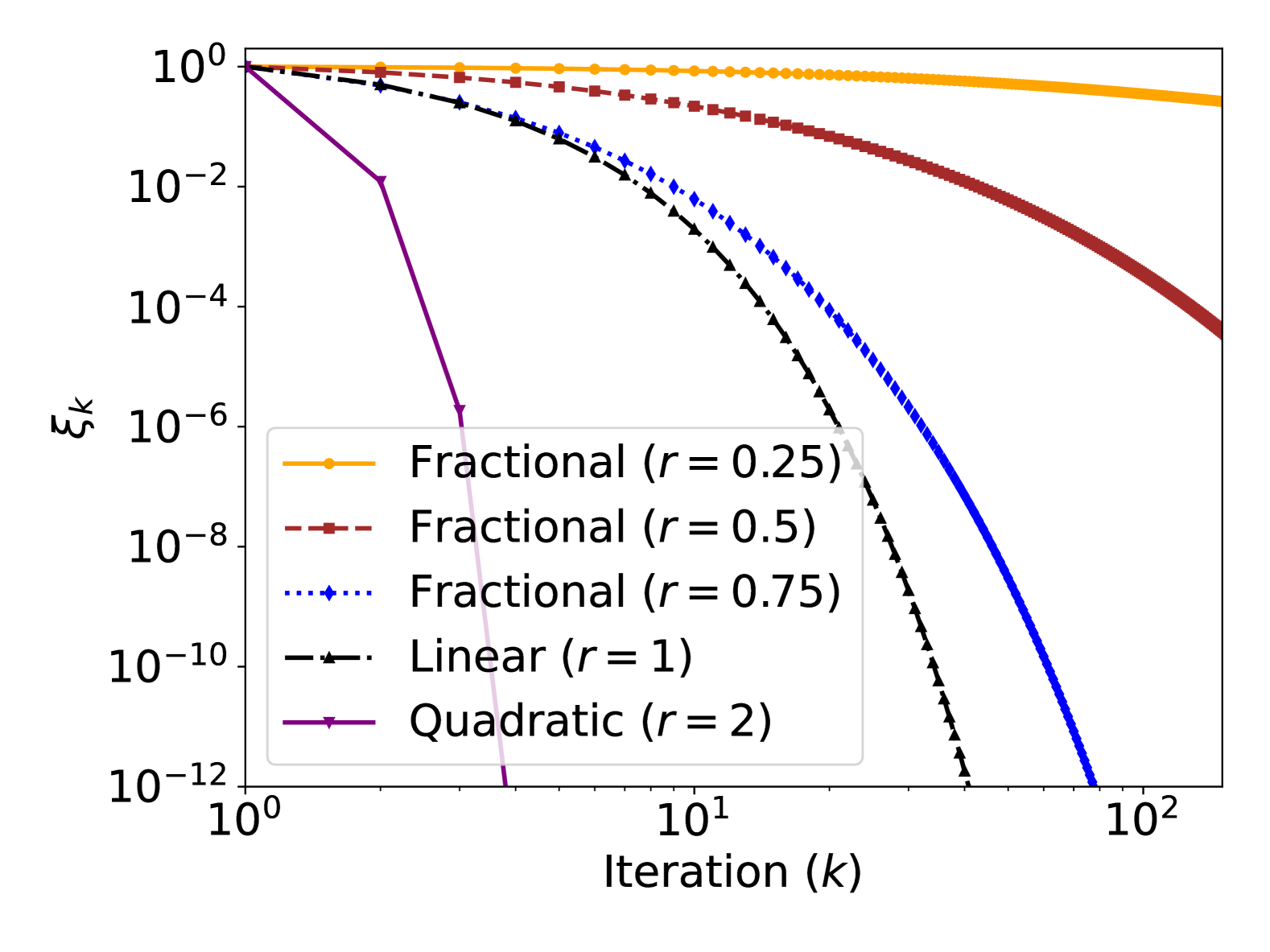
Figure 3: Examples of sublinear fractional-power rates of Newton’s method.

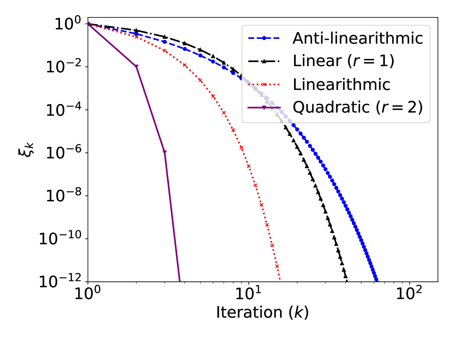
Figure 4: Examples of (anti-)linearithmic rates of Newton’s method.

5.2 Linearithmic and Anti-Linearithmic Convergence

We now present examples of linearithmic and anti-linearithmic convergence (as shown in Figure 4), which have not been studied previously in the literature. These examples are significant because they show that an iterative method may converge superlinearly but asymptotically slower than any exponential (or even polynomial) P-order, or converge sublinearly but be asymptotically faster than any fractional-power P-order. Understanding them helps us appreciate not only the power of the P-order framework but also the pitfalls of the previous frameworks as noted in 2.2.

Example 5.2 (Linearithmic Convergence).

We define the function

(35) $$f(x)=\begin{cases}|x-\alpha|\,\exp\!\Bigl{(}-\frac{1}{2}\Bigl{(}\ln(-\ln|x-\alpha|)\Bigr{)}^{2}\Bigr{)},&x\neq\alpha,\\[4.30554pt] 0,&x=\alpha,\end{cases}$$

so that $f(\alpha)=0$ for some $\alpha\in\mathbb{R}$. As in 5.1, this function is infinitely differentiable but not analytic at $\alpha$. Applying Newton’s method to solve $f(x)=0$ yields the iteration (33). For $x$ near $\alpha$, set $\epsilon=|x-\alpha|$. Note that

$$f(x)\sim\epsilon\,\exp\!\Bigl{(}-\frac{1}{2}\Bigl{(}\ln(-\ln\epsilon)\Bigr{)}^{2}\Bigr{)}.$$

A convenient way to analyze the update is to introduce $t(x)=\ln f(x)$. Then

$$g(x)=x-\frac{1}{t^{\prime}(x)},$$

and a careful asymptotic derivation shows that, for $\epsilon\to 0$,

$$t^{\prime}(x)\sim\operatorname{sign}(x-\alpha)\frac{-\ln\epsilon+\ln(-\ln\epsilon)}{\epsilon\,(-\ln\epsilon)}.$$

Inverting this relation leads to

$$\frac{g(x)-\alpha}{x-\alpha}\sim\frac{1}{k},$$

with the identification

$$k\sim\frac{-\ln\epsilon}{\ln(-\ln\epsilon)}.$$

In other words, if we define the error at the $k$th iteration by $\epsilon_{k}=|x_{k}-\alpha|$, then asymptotically

$$\epsilon_{k+1}\sim\frac{\epsilon_{k}}{k}.$$

Iterating this recurrence yields

$$\epsilon_{k}\sim\epsilon_{0}\prod_{j=1}^{k-1}\frac{1}{j}=\epsilon_{0}\,\frac{1}{(k-1)!}.$$

Taking logarithms and using Stirling’s approximation shows that

$$\epsilon_{k}=\Theta\Bigl{(}C^{\,k\ln k}\Bigr{)}$$

for some constant $C\in(0,1)$, thereby establishing the linearithmic convergence rate.

Example 5.3 (Anti-Linearithmic Convergence).

Consider the function

(36) $$f(x)=\begin{cases}|x-\alpha|^{\,\ln(-\ln|x-\alpha|)-1},&x\neq\alpha,\\[4.30554pt] 0,&x=\alpha,\end{cases}$$

so that $f(\alpha)=0$. As before, this function is infinitely differentiable but not analytic at $\alpha$. For $x$ near $\alpha$, set $\epsilon=|x-\alpha|$. In this case, we have

$$f(x)\sim\epsilon^{\,\ln(-\ln\epsilon)-1}.$$

As in 5.2, we introduce the auxiliary function $t(x)=\ln f(x)$, leading to $g(x)=x-1/t^{\prime}(x)$, where

$$t^{\prime}(x)\sim\operatorname{sign}(x-\alpha)\frac{\ln(-\ln\epsilon)}{\epsilon}$$

for $\epsilon\to 0$. Inverting this relation yields

$$\frac{g(x)-\alpha}{x-\alpha}\sim e^{-1/\ln k}\sim 1-\frac{1}{\ln k}.$$

with the identification

$$k\sim\frac{-\ln\epsilon}{\ln(-\ln\epsilon)}.$$

Denoting the error at the $k$th iteration by $\epsilon_{k}=|x_{k}-\alpha|$, we then obtain the asymptotic relation

$$\epsilon_{k+1}\sim\epsilon_{k}\Bigl{(}1-\frac{1}{\ln k}\Bigr{)}.$$

Iterating this recurrence leads to

$$\epsilon_{k}\sim\epsilon_{0}\,\exp\!\Bigl{(}-\frac{k}{\ln k}\Bigr{)}.$$

Taking logarithms and applying asymptotic approximations shows that

$$\epsilon_{k}=\Theta\Bigl{(}C^{\,k/\ln k}\Bigr{)},$$

where $C\in(0,1)$, thereby establishing the anti-linearithmic convergence rate.

To demonstrate the actual effects of linearithmic and anti-linearithmic convergence rates, we present numerical experiments in Figure Figure 4, where we applied Newton’s method to solve special cases in 5.2 and 5.3 with $\alpha=0$, i.e.,

$$f(x)=xe^{-\frac{1}{2}(\ln(-\ln x))^{2}}$$

and

$$f(x)=x^{\,\ln(-\ln x)-1}.$$

It is clear that the linearithmic convergence rate is a little faster than linear convergence but much slower than quadratic convergence, while the anti-linearithmic rate is a little slower than but very close to linear convergence. These results match our theoretical analyses in 5.2 and 5.3.

6 Conclusions and Discussions

In this paper, we introduced P-order, a unified, norm-independent framework for analyzing the convergence rates of multivariate iterative methods. P-order generalizes and refines classical concepts like Q-order and R-order by parameterizing the convergence rate with an increasing power function, $\psi(k)$. A particularly convenient subclass, QUP-order, is more general and easier to apply than Q-order, and is the primary focus of this paper. A key result is the refined analysis of near-linear and sublinear convergence, including fractional-power, logarithmic, linearithmic, and anti-linearithmic rates, enabling a more precise characterization of methods where error decay is nearly linear or slower. We demonstrated the application of P-order to the analysis of general fixed-point iterations and Newton’s method. For fixed-point iterations, we established conditions under which different P-orders (including sublinear fractional power) of convergence rates are achieved. For Newton’s method, we presented a refined analysis of its convergence behavior, including sublinear fractional-power, linearithmic, and anti-linearithmic rates, which have not been reported in the literature. This result provides a more comprehensive understanding of the convergence behavior of Newton’s method, especially near singular roots.

While the focus of this work is on establishing a mathematically rigorous framework for analyzing convergence rates of iterative methods, it is by no means a purely theoretical exercise. By providing a more precise characterization of the convergence behavior of iterative methods, the P-order framework has practical implications for the design and analysis of iterative methods in scientific computing and machine learning. For example, many iterative methods, such as (stochastic) gradient descent and subgradient methods in numerical optimization, exhibit sublinear convergence rates. A more refined analysis of their sublinear convergence behavior can provide a better understanding of their convergence properties and guide the development of new algorithms with improved convergence rates. To this end, we plan to extend the P-order framework to analyze stochastic methods, such as stochastic gradient descent (SGD), and to study the convergence behavior of their variants in future work.

Appendix A Q-Superlinear Implies UP-Superlinear

Proof A.1 (Proof of Theorem 3.4).

Define

$$\xi_{k}=\|\boldsymbol{x}_{k}-\boldsymbol{x}_{*}\|,\quad f(k)=-\ln\xi_{k}.$$

By Q-superlinear convergence,

$$\lim_{k\to\infty}\frac{\xi_{k+1}}{\xi_{k}^{q}}=Q_{q},\quad q>1,\quad 0<Q_{q}<\infty.$$

Taking logarithms, define

(37) $$d(k)=f(k+1)-qf(k)=-\ln\Bigl{(}\frac{\xi_{k+1}}{\xi_{k}^{q}}\Bigr{)}.$$

Then

$$\lim_{k\to\infty}d(k)=-\ln Q_{q}\coloneqq d,$$

so that $\{d(k)\}$ is bounded; i.e., there exists $M>0$ with $|d(k)|\leq M$.

Unrolling the recurrence

$$f(k+1)=qf(k)+d(k)$$

yields

$$f(k)=q^{\,k-1}f(1)+\sum_{j=1}^{k-1}q^{\,k-1-j}d(j).$$

Dividing by $q^{k}$, we have

$$\frac{f(k)}{q^{k}}=\frac{f(1)}{q}+\sum_{j=1}^{k-1}\frac{d(j)}{q^{\,j+1}}.$$

Since the tail of the series is bounded by

$$\sum_{j=k}^{\infty}\frac{|d(j)|}{q^{\,j+1}}\leq M\sum_{j=k}^{\infty}\frac{1}{q^{\,j+1}},$$

the limit

(38) $$s=\lim_{k\to\infty}\frac{f(k)}{q^{k}}=\frac{f(1)}{q}+\sum_{j=1}^{\infty}\frac{d(j)}{q^{\,j+1}}$$

exists and satisfies $s>0$ (since for large $j$, $d(j)$ remains bounded away from zero).

Thus, we can write

$$f(k)=sq^{k}+\mathcal{O}(1),$$

so that

$$\xi_{k}=e^{-f(k)}=e^{-sq^{k}}\,e^{-\mathcal{O}(1)}.$$

That is, there exist constants $A,B>0$ with

$$A\,e^{-sq^{k}}\leq\xi_{k}\leq B\,e^{-sq^{k}}.$$

Defining

$$C_{\psi}=e^{-s}\quad(0<C_{\psi}<1),$$

we obtain

$$A\,C_{\psi}^{q^{k}}\leq\xi_{k}\leq B\,C_{\psi}^{q^{k}},$$

which is equivalent to UP-superlinear convergence with P-function $\psi(k)=q^{k}$.

Appendix B Proof of Quadratic and Higher-Order Convergence of Fixed-Point Iteration

Proof B.1 (Proof of 2).

Let $\boldsymbol{\xi}_{k}=\boldsymbol{x}_{k}-\boldsymbol{x}_{*}$ and, for $\boldsymbol{\xi}_{k}\neq\boldsymbol{0}$, define

$$\boldsymbol{v}_{k}=\frac{\boldsymbol{\xi}_{k}}{\|\boldsymbol{\xi}_{k}\|}.$$

By hypothesis (29), the directional Taylor expansion of $\boldsymbol{g}$ at $\boldsymbol{x}_{*}$ along $\boldsymbol{v}_{k}$ yields

$$\boldsymbol{g}(\boldsymbol{x}_{k})=\boldsymbol{x}_{*}+\frac{1}{q!}\,\partial^{(q)}_{\boldsymbol{v}_{k}}\boldsymbol{g}(\boldsymbol{x}_{*})\,\|\boldsymbol{\xi}_{k}\|^{q}+\boldsymbol{r}\bigl{(}\|\boldsymbol{\xi}_{k}\|\bigr{)},$$

where the remainder $\boldsymbol{r}\bigl{(}\|\boldsymbol{\xi}_{k}\|\bigr{)}$ satisfies $\|\boldsymbol{r}\bigl{(}\|\boldsymbol{\xi}_{k}\|\bigr{)}\|=o\bigl{(}\|\boldsymbol{\xi}_{k}\|^{q}\bigr{)}$. Since $\boldsymbol{g}(\boldsymbol{x}_{*})=\boldsymbol{x}_{*}$, using the Peano form under the assumption of $q$-times continuous differentiability of $\boldsymbol{g}$, we have

$$\boldsymbol{\xi}_{k+1}=\frac{1}{q!}\,\partial^{(q)}_{\boldsymbol{v}_{k}}\boldsymbol{g}(\boldsymbol{x}_{*})\,\|\boldsymbol{\xi}_{k}\|^{q}+o\bigl{(}\|\boldsymbol{\xi}_{k}\|^{q}\bigr{)}.$$

By the general position assumption and the hypothesis (30), there exist constants $A,B>0$ such that for all sufficiently small $\|\boldsymbol{\xi}_{k}\|$,

$$A\,\|\boldsymbol{\xi}_{k}\|^{q}\leq\|\boldsymbol{\xi}_{k+1}\|\leq B\,\|\boldsymbol{\xi}_{k}\|^{q}.$$

Taking logarithms, let

$$a_{k}=\ln\|\boldsymbol{\xi}_{k}\|.$$

Then the above inequality implies

$$\ln A+q\,a_{k}\leq a_{k+1}\leq\ln B+q\,a_{k}.$$

This linear recurrence in $a_{k}$ can be solved by induction. In particular, there exist constants $C_{1}$ and $C_{2}$ (depending on $a_{K}$ for some fixed index $K$) such that for all $k\geq K$

$$C_{1}+q^{\,k-K}\,a_{K}\leq a_{k}\leq C_{2}+q^{\,k-K}\,a_{K}.$$

Exponentiating these bounds, we obtain

$$e^{C_{1}}\,\|\boldsymbol{\xi}_{K}\|^{\,q^{\,k-K}}\leq\|\boldsymbol{\xi}_{k}\|\leq e^{C_{2}}\,\|\boldsymbol{\xi}_{K}\|^{\,q^{\,k-K}}.$$

Since $\|\boldsymbol{\xi}_{K}\|$ is fixed (depending on the initial error $\|\boldsymbol{\xi}_{0}\|$), we may absorb it into the constants. Thus, there exist constants $\widetilde{C}_{1},\widetilde{C}_{2}>0$ such that for all sufficiently large $k$

$$\widetilde{C}_{1}\,\|\boldsymbol{\xi}_{0}\|^{\,q^{k}}\leq\|\boldsymbol{\xi}_{k}\|\leq\widetilde{C}_{2}\,\|\boldsymbol{\xi}_{0}\|^{\,q^{k}}.$$

By the definition of P-order, this shows that the sequence $\{\boldsymbol{x}_{k}\}$ converges to $\boldsymbol{x}_{*}$ with P-order $q$.

Appendix C Proof of Fractional-Power Convergence Rate of Fixed-Point Iteration

Proof C.1 (Proof of 3).

Let $\boldsymbol{\xi}_{k}=\boldsymbol{x}_{k}-\boldsymbol{x}_{*}$ denote the error vector. Decompose

$$\boldsymbol{\xi}_{k}=\boldsymbol{P}_{\rho}\,\boldsymbol{\xi}_{k}+\boldsymbol{Q}_{\rho}\,\boldsymbol{\xi}_{k},$$

where $\boldsymbol{P}_{\rho}$ is the projection onto the generalized eigenspace $\mathcal{E}_{\rho}$ (corresponding to eigenvalues of modulus one) and $\boldsymbol{Q}_{\rho}=\boldsymbol{I}-\boldsymbol{P}_{\rho}$. By hypothesis, there exists $\gamma\in[0,1)$ such that

$$\|\boldsymbol{Q}_{\rho}\,\boldsymbol{\xi}_{k}\|=\mathcal{O}(\gamma^{k}).$$

Define

$$u_{k}=\|\boldsymbol{P}_{\rho}\,\boldsymbol{\xi}_{k}\|.$$

The assumption guarantees that for $\boldsymbol{x}=\boldsymbol{x}_{k}$ sufficiently close to $\boldsymbol{x}_{*}$, for any $\epsilon>0$ there exists an index $k_{1}$ such that

$$u_{k}\Bigl{(}1-(C_{0}+\epsilon)\,(-\ln u_{k})^{-s}\Bigr{)}\leq u_{k+1}\leq u_{k}\Bigl{(}1-(C_{0}-\epsilon)\,(-\ln u_{k})^{-s}\Bigr{)}.$$

Introduce the transformation $v_{k}=-\ln u_{k}$ so that $u_{k}=e^{-v_{k}}$. Then, there exists $k_{2}\geq k_{1}$, for all $k\geq k_{2}$,

$$v_{k}+(C_{0}-\epsilon)\,v_{k}^{-s}\leq v_{k+1}\leq v_{k}+(C_{0}+\epsilon)\,v_{k}^{-s},$$

(obtained via the expansion $\ln(1-x)=-x+\mathcal{O}(x^{2})$ as $x\to 0$).

We first show that there exists an index $K\geq k_{2}$ such that

(39) $$\limsup_{k\rightarrow\infty}\frac{v_{k}}{k^{1/(s+1)}}\leq((C_{0}+\epsilon)(s+1))^{\frac{1}{s+1}}\,,\quad\forall\,k\geq K.$$

Write $w(k)=v_{k}^{s+1}$, then by the Mean Value Theorem,

$$w(k+1)-w(k)=v_{k+1}^{s+1}-v_{k}^{s+1}=(s+1)\xi_{k}^{s}(v_{k+1}-v_{k})\leq(s+1)(C_{0}+\epsilon)\frac{\xi_{k}^{s}}{v_{k}^{s}},$$

where $v_{k}\leq\xi_{k}\leq v_{k+1}$. Since $\xi_{k}\leq v_{k+1}\leq v_{k}+(C_{0}+\epsilon)v_{k}^{-s}$, we have $\xi_{k}^{s}/v_{k}^{s}\leq(1+(C_{0}+\epsilon)v_{k}^{-s-1})^{s}$. For any $\delta>0$, there exists $N>0$ such that $\xi_{k}^{s}/v_{k}^{s}<1+\delta$ for any $k>N$. Hence, for any $k>N$,

$$w(k+1)-w(k)\leq(s+1)(C_{0}+\epsilon)(1+\delta).$$

Hence, it is clear that

$$\lim_{k\rightarrow\infty}\frac{w(k)}{k(s+1)(C_{0}+\epsilon)(1+\delta)}\leq 1.$$

Note that this conclusion applies to any $\delta>0$, and thus we actually have

$$\lim_{k\rightarrow\infty}\frac{v_{k}^{s+1}}{k(s+1)(C_{0}+\epsilon)}=\lim_{k\rightarrow\infty}\frac{w(k)}{k(s+1)(C_{0}+\epsilon)}\leq 1.$$

Thus, we have

$$\limsup_{k\rightarrow\infty}\frac{v_{k}}{k^{1/(s+1)}}\leq((s+1)(C_{0}+\epsilon))^{1/(1+s)}$$

for any $\epsilon>0$. By a similar argument, we can also show that

$$\liminf_{k\rightarrow\infty}\frac{v_{k}}{k^{1/(s+1)}}\geq((s+1)(C_{0}-\epsilon))^{1/(1+s)}$$

for any $\epsilon>0$. By the Squeeze Theorem, we obtain

(40) $$\lim_{k\rightarrow\infty}\frac{v_{k}}{k^{1/(s+1)}}=(C_{0}(s+1))^{1/(1+s)}.$$

Moreover, the full error satisfies

$$\|\boldsymbol{\xi}_{k}\|=u_{k}+r_{k},$$

where

$$r_{k}=\|\boldsymbol{Q}_{\rho}\,\boldsymbol{\xi}_{k}\|=\mathcal{O}(\gamma^{k}).$$

Because $u_{k}=e^{-v_{k}}$ decays subexponentially (i.e., as $e^{-C_{0}\,k^{1/(s+1)}}$) while $r_{k}$ decays exponentially, it follows that

$$\lim_{k\to\infty}\frac{\|\boldsymbol{\xi}_{k}\|}{u_{k}}=1.$$

Thus,

$$\lim_{k\to\infty}\|\boldsymbol{\xi}_{k}\|^{k^{-1/(s+1)}}=\lim_{k\to\infty}u_{k}^{k^{-1/(s+1)}}=\lim_{k\to\infty}e^{-v_{k}/k^{1/(s+1)}}=e^{-(C_{0}(s+1))^{1/(s+1)}}\eqcolon C_{\psi},$$

where $C_{\psi}\in(0,1)$. This completes the proof that the iteration converges with QUP-order $r=1/(s+1)$, which is sublinear a fractional-power rate.

References

- [1] S. Banach, Sur les opérations dans les ensembles abstraits et leur application aux équations intégrales, Fundam. Math., 3 (1922), pp. 133–181.
- [2] L. Bottou, F. E. Curtis, and J. Nocedal, Optimization methods for large-scale machine learning, SIAM Rev., 60 (2018), pp. 223–311.
- [3] C. Brezinski, Comparaison de suites convergentes, Rev. Fr. Inform. Rech. Oper., 2 (1971), pp. 95–99.
- [4] D. Carvalho, F. S. Melo, and P. Santos, A new convergent variant of Q-learning with linear function approximation, Adv. Neural Inf. Process. Syst., 33 (2020), pp. 19412–19421.
- [5] T. H. Cormen, C. E. Leiserson, R. L. Rivest, and C. Stein, Introduction to Algorithms, MIT Press, 3rd ed., 2009.
- [6] D. W. Decker, H. B. Keller, and C. T. Kelley, Convergence rates for Newton’s method at singular points, SIAM J. Numer. Anal., 20 (1983), pp. 296–314.
- [7] D. W. Decker and C. T. Kelley, Newton’s method at singular points. I, SIAM J. Numer. Anal., 17 (1980), pp. 66–70.
- [8] J. Dennis, J. E. and R. B. Schnabel, Numerical Methods for Unconstrained Optimization and Nonlinear Equations, Prentice-Hall, 1983. Republished by SIAM, 1996.
- [9] A. Griewank, On solving nonlinear equations with simple singularities or nearly singular solutions, SIAM Rev., 27 (1985), pp. 537–563.
- [10] L. O. Jay, A note on Q-order of convergence, BIT Numer. Math., 42 (2002), pp. 370–378.
- [11] L. Kantorovich, Functional analysis and applied mathematics, Uspekhi Mat. Nauk, 3 (1948), pp. 89–185.
- [12] D. E. Knuth, The Art of Computer Programming, vol. 1, Addison-Wesley, 3rd ed., 1997.
- [13] A. Nemirovski, A. Juditsky, G. Lan, and A. Shapiro, Robust stochastic approximation approach to stochastic programming, SIAM J. Optim., 19 (2009), pp. 1574–1609.
- [14] J. Nocedal and S. J. Wright, Numerical Optimization, Springer, 2nd ed., 2006.
- [15] J. M. Ortega, Numerical Analysis: A Second Course, Academic Press, New York, 1972. Reprinted by SIAM, Philadelphia, 1990.
- [16] J. M. Ortega and W. C. Rheinboldt, Iterative Solution of Nonlinear Equations in Several Variables, Academic Press, 1970. Republished by SIAM, Philadelphia, 2000.
- [17] A. M. Ostrowski, Solution of Equations and Systems of Equations, Academic Press, New York, 2nd ed., 1966.
- [18] F. A. Potra, On Q-order and R-order of convergence, J. Optim. Theory Appl., 63 (1989), pp. 415–431.
- [19] F. A. Potra and V. Pták, Nondiscrete Induction and Iterative Processes, Pitman, Boston, Massachusetts, 1984.
- [20] L. B. Rall, Convergence of the Newton process to multiple solutions, Numer. Math., 9 (1966), pp. 23–37.
- [21] S. J. Reddi, S. Kale, and S. Kumar, On the convergence of adam and beyond, in International Conference on Learning Representations, 2018.
- [22] G. W. Reddien, On Newton’s method for singular problems, SIAM J. Numer. Anal., 15 (1978), pp. 993–996.
- [23] H. Schwetlick, Numerische Lösung Nichtlinearer Gleichungen, VEB, Berlin, Germany, 1979.
- [24] W. Sun and Y.-X. Yuan, Optimization Theory and Methods: Nonlinear Programming, vol. 1, Springer, 2006.
- [25] J. F. Traub, Iterative Methods for the Solution of Equations, Prentice-Hall, Englewood Cliffs, NJ, 1964. Reprinted by Chelsea Publishing Company, 1982; Reprinted by AMS Chelsea Publishing, 2016.