Over-Relaxation in Alternating Projections

Abstract

We improve upon the current bound on convergence rates of the Gauss-Seidel, Kaczmarz, and more generally projection methods where projections are visited in randomized order. The tighter bound reveals a practical approach to speed up convergence by over-relaxation — a longstanding challenge that has been difficult to overcome for general problems with deterministic Succession of Over-Relaxations.

1 Projection Methods

Iterative methods use a projection as a canonical way to extract an improvement towards the solution in each step. Most standard techniques can be viewed as a succession of such projections. The Gauss-Seidel and Kaczmarz are prominent examples of projection methods with a wide range of applications in scientific computing, machine learning, biomedical imaging and signal processing.

Solving $m$ equations with $n$ unknowns forming the system ${\boldsymbol{A}}{{\bf x}}={{\bf b}}$, the iterations start from an initial guess ${{\bf x}}_{0}$ and evolve towards the solution as in Figure 1. In the $k^{\rm th}$ step of iterations, a coordinate, $i$, of the residual ${{\bf b}}-{\boldsymbol{A}}{{\bf x}}_{k}$ is chosen to update the iterate, ${{\bf x}}_{k}$, along a vector ${\bf d}_{i}$ from a predetermined set:

$${{\bf x}}_{k+1}={{\bf x}}_{k}+\omega\frac{{{\bf e}}_{i}^{T}({{\bf b}}-{\boldsymbol{A}}{{\bf x}}_{k})}{\lVert{\bf d}_{i}\rVert^{2}}{\bf d}_{i}.$$ (1)

Here ${{\bf e}}_{i}$ is the standard coordinate vector enabling calculation of ${{\bf e}}_{i}^{T}({{\bf b}}-{\boldsymbol{A}}{{\bf x}}_{k})$ with $O(n)$ floating point operations and $\omega\in(0,2)$ is a relaxation parameter. In the Gauss-Seidel method the iterate is simply updated along coordinates (hence called a coordinate descent method) ${\bf d}_{i}:={{\bf e}}_{i}$ together with the ${\boldsymbol{A}}$-induced norm: $\lVert{\bf d}_{i}\rVert^{2}:={{\bf e}}_{i}^{T}{\boldsymbol{A}}{{\bf e}}_{i}={\boldsymbol{A}}_{ii}$. In the Kaczmarz method the iterate is updated along the $i^{\rm th}$ row of ${\boldsymbol{A}}$: ${\bf d}_{i}:={\boldsymbol{A}}^{T}{{\bf e}}_{i}$ and $\lVert\cdot\rVert$ denotes the standard Euclidean norm.

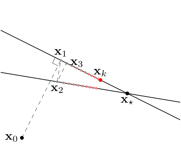
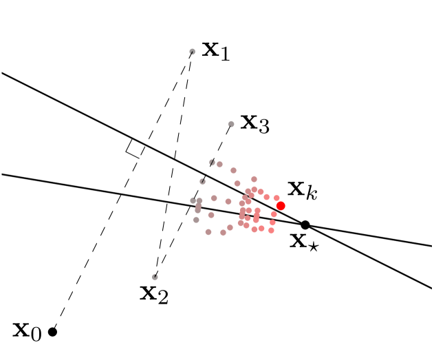
Figure 1: Alternating Projections: At each step, one of the $m=2$ projections is chosen, at random. Left figure shows the trajectory for $\omega=1$ where we, greedily, minimize the error in each step. The right figure shows the over-relaxation trajectory for $\omega=1.5$ exhibiting faster convergence. The method of Successive Over-Relaxations (SOR) was devised by David Young in 1950 improving convergence rate of Gauss-Seidel for diagonally dominant matrices appearing in elliptic PDE problems. This paper shows that by randomizing the order, instead of cycles with a pre-determined order, the over-relaxation phenomenon occurs in general problems, and can be leveraged to speed up convergence.

2 Contribution and Related Work

Convergence of the Gauss-Seidel method is guaranteed for a symmetric positive definite ${\boldsymbol{A}}$ (representing $m=n$ equations). More broadly, given $m\geq n$ consistent equations forming ${\boldsymbol{A}}$, the Kaczmarz algorithm is guaranteed to converge to a point ${{\bf x}}_{\star}$ that satisfies the equations. From a practical viewpoint, the key questions about these methods are:

• What is the geometric rate of convergence, $\rho(\omega)$, and what properties of ${\boldsymbol{A}}$ determine this rate?

• How can one pick the relaxation parameter, $\omega$, to minimize $\rho(\omega)$ and speed up convergence?

We introduce a new approach to analyze the performance of alternating projections that not only provides tighter bounds, on $\rho(\omega)$, than what is currently known about the rate of convergence, but more importantly reveals a practical way to select an over-relaxation parameter, $\omega>1$, that is guaranteed to speed up convergence. To place these developments in perspective, we first discuss existing mathematical tools for analysis.

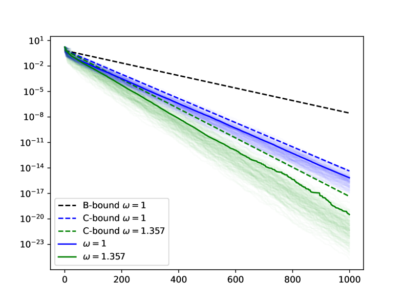
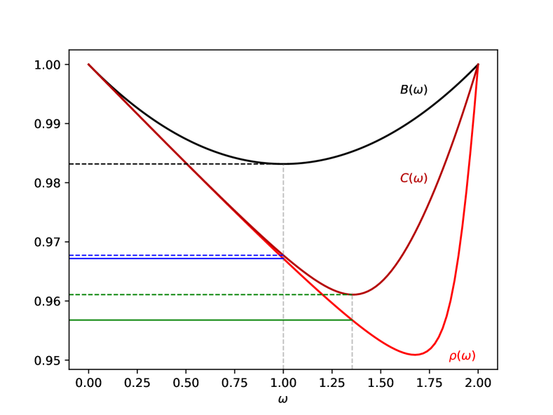
Figure 2: Left: Empirical study of a toy problem with $m=n=5$: instead of forward/backward sweeps, at each step of (1), $i$ was randomly chosen from $\{1,\dots,5\}$ with uniform probability. Blue visualizes the errors (in log scale) of 150 trials for 1000 iterations without relaxation ($\omega=1$). The solid blue shows the mean of trials whose slope depicts the empirical rate of convergence. The dashed black line, we call B-bound, shows the current bound, to the solid blue, obtained from a Markovian analysis of the error norm, which is well known to be loose in practice. The dashed blue shows the new bound, we call the C-bound, that traces the mean (solid blue) closely. Green plots show the improved performance due to over-relaxation resulting from our analysis. Right: $\rho(\omega)$ shows the true convergence rate determined from the spectral radius of a certain superoperator — playing the role of the iteration matrix — as a function of the relaxation parameter. The B-bound, $B(\omega)$, is based on the smallest singular value of ${\boldsymbol{A}}$, and the C-bound, $C(\omega)$, is based on the two smallest singular values that provide bounds for $\rho(\omega)$. Our analysis shows the improvement in the C-bound and the resulting over-relaxation depends on the gap between the two smallest singular values and a geometric measure of orthogonality of ${\boldsymbol{A}}$.

Notation

We use bold lower case characters to denote vectors (e.g., ${{\bf x}}\in\mathbb{R}^{n}$ and ${{\bf b}}\in\mathbb{R}^{m}$), and bold upper case characters to denote matrices representing linear transformations on $\mathbb{R}^{n}$ (e.g., ${\boldsymbol{A}}\in\mathbb{R}^{m\times n}$). The eigenvalues of a symmetric matrix (operator), $\boldsymbol{M}$, are indexed from low to high:

$$\lambda_{\min}(\boldsymbol{M}):=\lambda_{1}(\boldsymbol{M})\leq\lambda_{2}(\boldsymbol{M})\leq\cdots\leq\lambda_{\max}(\boldsymbol{M}).$$

That index also denotes the corresponding eigenvectors: $\boldsymbol{M}{\bf v}_{i}(\boldsymbol{M})=\lambda_{i}(\boldsymbol{M}){\bf v}_{i}(\boldsymbol{M})$. The calligraphic font is used to denote superoperators or linear maps over the vector space of $n\times n$ matrices. The eigenvectors and eigenvalues of a superoperator, $\boldsymbol{\mathcal{M}}$, are denoted accordingly: $\boldsymbol{\mathcal{M}}\left(\boldsymbol{V}_{i}(\boldsymbol{\mathcal{M}})\right)=\lambda_{i}(\boldsymbol{\mathcal{M}})\boldsymbol{V}_{i}(\boldsymbol{\mathcal{M}})$. In this vector space, we denote the Frobenius inner product by $\langle\boldsymbol{M},\boldsymbol{M}^{\prime}\rangle:=\operatorname{tr}\left(\boldsymbol{M}^{T}\boldsymbol{M}^{\prime}\right)$.

2.1 Convergence Analysis

Analyzing convergence, one can view these iterations as a sequence of projections. Defining a vector $\boldsymbol{\varepsilon}_{k}$ that defines a notion of error one can show that iterations shrink $\boldsymbol{\varepsilon}_{k}$ by projecting it to a set of subspaces. For Kaczmarz, this is simply the error vector $\boldsymbol{\varepsilon}_{k}:={{\bf x}}_{k}-{{\bf x}}_{\star}$ and for Gauss-Seidel, $\boldsymbol{\varepsilon}_{k}:={\boldsymbol{A}}^{1/2}({{\bf x}}_{k}-{{\bf x}}_{\star})$. Then iterations in (1) can be viewed as a succession of projections:

$$\boldsymbol{\varepsilon}_{k+1}=(\boldsymbol{I}-\omega\boldsymbol{P}_{i})\boldsymbol{\varepsilon}_{k},$$ (2)

where $\boldsymbol{P}_{i}$ denotes the projector onto a subspace spanned by the $i^{th}$ row of ${\boldsymbol{A}}^{1/2}$ for Gauss-Seidel and the $i^{th}$ row of ${\boldsymbol{A}}$ for Kaczmarz. When visiting individual rows in each step of (1), the iterate is projected onto hyperplanes, but visiting a block of rows in each step leads to projectors to subspaces with larger co-dimensions.

The convergence of iterations to a point ${{\bf x}}_{\star}$ at the intersection of hyperplanes can be established for $\omega\in(0,2)$ based on the contraction that $\boldsymbol{I}-\omega\boldsymbol{P}_{i}$ introduces (Herman et al., 1978) in each step. This contraction occurs for any choice, deterministic or random, of order in which the equations are visited. The question of convergence rate, however, does not have a simple answer.

Convergence Rate

The fundamental difficulty in deriving the rate of convergence for (2) lies in the geometric nature of iterations (Censor et al., 2009). It is well known that the rate of convergence not only depends on angles between subspaces these projectors represent, but more importantly on the order these subspaces are visited (Deutsch, 1995; Galántai, 2005). In other words, the order in which rows of ${\boldsymbol{A}}$ are visited (i.e., choice of $i$ for each step) has a major impact on the rate of convergence. This geometric difficulty can be approached algebraically with an eigenvalue problem (spectral radius) in certain cases as we describe next.

2.2 Successive Projections – Deterministic Order

Once an order is fixed among the $m$ equations that form ${\boldsymbol{A}}$, the iterations use this order for picking $i$ to cyclically sweep through equations (forward or backward). This process allows for introducing an iteration matrix ${\boldsymbol{G}}$ that describes the evolution of error after a full sweep through $m$ steps of (1):

$$\boldsymbol{\varepsilon}_{m(k+1)}={\boldsymbol{G}}\boldsymbol{\varepsilon}_{mk}\quad{\rm with}\quad{\boldsymbol{G}}:=\prod_{i=1}^{m}{(\boldsymbol{I}-\omega\boldsymbol{P}_{i})}.$$ (3)

The iteration matrix ${\boldsymbol{G}}$, in turn, determines the rate of convergence for the cyclic iterations (Saad, 2003). More specifically, its spectral radius (i.e., largest eigenvalue) determines the asymptotic convergence rate: $\rho(\omega)=\lambda_{\max}({\boldsymbol{G}})$. Nevertheless, this rate is specific to the order in which the equations are arranged in ${\boldsymbol{A}}$ — which is one of the $m!$ many possibilities.

The iteration matrix for Gauss-Seidel ($m=n$) turns out to have a convenient form. It can be built from a diagonal matrix $\boldsymbol{D}$ that matches the diagonal of ${\boldsymbol{A}}$ and a lower triangular matrix $\boldsymbol{E}$ that matches the lower triangular part of $-{\boldsymbol{A}}$. One can show that a forward sweep of $m$ steps in (1) results in:

$${{\bf x}}_{m(k+1)}-{{\bf x}}_{\star}=\left(\boldsymbol{I}-\omega(\boldsymbol{D}-\omega\boldsymbol{E})^{-1}{\boldsymbol{A}}\right)({{\bf x}}_{mk}-{{\bf x}}_{\star}).$$

This means ${\boldsymbol{A}}^{-1/2}{\boldsymbol{G}}{\boldsymbol{A}}^{1/2}=\boldsymbol{I}-\omega(\boldsymbol{D}-\omega\boldsymbol{E})^{-1}{\boldsymbol{A}}$ that share eigenvalues $\lambda({\boldsymbol{G}})=\lambda({\boldsymbol{A}}^{-1/2}{\boldsymbol{G}}{\boldsymbol{A}}^{1/2})$. Hence the convergence rate is determined from the smallest eigenvalue of $(\boldsymbol{D}-\omega\boldsymbol{E})^{-1}{\boldsymbol{A}}$ that is directly constructed from ${\boldsymbol{A}}$. Nevertheless, the question of over-relaxation in general proves difficult and can only be studied for matrices that satisfy special structural conditions (Young, 1954; Hackbusch, 2016).

Although the iteration matrix for Kaczmarz can be constructed from ${\boldsymbol{A}}$ as the product in (3), it remains inscrutable since its relationship to properties of ${\boldsymbol{A}}$ is opaque. When $\omega=1$ (i.e., no relaxation), the convergence of the alternating projections has been well studied. In this context a bound on the rate of convergence (Halperin, 1962) can be computed based on a sequence of angles between subspaces as they appear in the sweep (Deutsch and Hundal, 1997; Smith et al., 1977; Kayalar and Weinert, 1988). These bounds are difficult to calculate (Galántai, 2005) and specific to the order in which equations are visited.

We note that the convergence rates of the Cimmino method and Richardson iterations are determined from the extrema of ${\boldsymbol{A}}$’s spectrum and so are the optimal over-relaxations (Saad, 2003). However these iterations require a full sweep through rows before ${{\bf x}}_{k}$ is updated and hence are inefficient compared to Kaczmarz and Gauss-Seidel in which ${{\bf x}}_{k}$ is updated in each step.

2.3 Alternating Projections – Randomized Order

As pointed out earlier, regardless of the order equations are visited, $\boldsymbol{I}-\omega\boldsymbol{P}_{i}$ induces a contraction in each step. The concept of randomizing the order in which equations are visited, can be traced back to the field of stochastic approximation. In this context for the, more general, least squares problem the stochastic gradient descent (SGD) method is referred to as the least mean squares (LMS) algorithm (Widrow and Hoff, 1988). This approach is also investigated in Incremental Gradient Methods (IGM) (Nedić and Bertsekas, 2001; Bertsekas, 2011). The behavior of SGD and its convergence regimes on the linear least squares problem is well studied (Solo, 1989; Polyak and Juditsky, 1992; Nemirovski et al., 2009; Aguech et al., 2000; Bach and Moulines, 2013; Défossez and Bach, 2015; Jain et al., 2018).

For a consistent set of equations ${\boldsymbol{A}}{{\bf x}}={{\bf b}}$, the convergence rate of the Kaczmarz algorithm, where rows of ${\boldsymbol{A}}$ are visited in a randomized order, was established in (Strohmer and Vershynin, 2009) whose results were extended to the Gauss-Seidel method (Leventhal and Lewis, 2010). These results sparked significant interest in machine learning and optimization (Nutini et al., 2009; Recht and Ré, 2012; Gower and Richtárik, 2015; Tu et al., 2017). While different sampling strategies have been explored, for large scale problems where these iterative methods become favorable over direct methods, the only viable choice of probabilities for sampling is uniform: $i$ in (1) is chosen with the uniform probability from $\{1,\dots,m\}$. Nevertheless, our analysis is applicable to any choice of probabilities.

The Expected Projector

A Markovian view of iterations provides a geometric convergence guarantee due to deterministic contraction (Hairer, 2006). To quantify the contraction rate, (Strohmer and Vershynin, 2009) analyzed the evolution of the norm (squared) of the error in one step from (2) as $\lVert\boldsymbol{\varepsilon}_{k+1}\rVert^{2}=\boldsymbol{\varepsilon}_{k}^{T}\left(\boldsymbol{I}-\omega(2-\omega)\boldsymbol{P}_{i}\right)\boldsymbol{\varepsilon}_{k}$. The expected error norm is evolved according to the expected projector:

$$\operatorname{\mathbb{E}}{\left[\lVert\boldsymbol{\varepsilon}_{k+1}\rVert^{2}\mid\boldsymbol{\varepsilon}_{k}\right]}=\boldsymbol{\varepsilon}_{k}^{T}\left(\boldsymbol{I}-\omega(2-\omega)\operatorname{\mathbb{E}}\left[\boldsymbol{P}\right]\right)\boldsymbol{\varepsilon}_{k}\quad{\rm with}\quad\operatorname{\mathbb{E}}\left[\boldsymbol{P}\right]:=\frac{1}{m}\sum_{i=1}^{m}{\boldsymbol{P}_{i}}.$$ (4)

Under uniform sampling, $\operatorname{\mathbb{E}}\left[\boldsymbol{P}\right]$ is directly related to ${\boldsymbol{A}}$: for the Gauss-Seidel method it is simply $\operatorname{\mathbb{E}}\left[\boldsymbol{P}\right]=\frac{1}{n}{\boldsymbol{A}}$ where ${\boldsymbol{A}}$ is normalized (scaling from left and right) to have unit diagonals, whereas in the Kaczmarz method $\operatorname{\mathbb{E}}\left[\boldsymbol{P}\right]$ is the Grammian of (the row normalized) ${\boldsymbol{A}}$: $\operatorname{\mathbb{E}}\left[\boldsymbol{P}\right]=\frac{1}{m}{\boldsymbol{A}}^{T}{\boldsymbol{A}}$. In particular, the spectrum of $\operatorname{\mathbb{E}}\left[\boldsymbol{P}\right]$ is a directly computable from the singular values of the normalized ${\boldsymbol{A}}$. Using the symbol $\mu$ to denote the eigenvalues of the expected projector with $\mu_{1}:=\lambda_{1}(\operatorname{\mathbb{E}}\left[\boldsymbol{P}\right])$ its smallest eigenvalue, one can bound the reduction of the expected error as $\operatorname{\mathbb{E}}{\left[\lVert\boldsymbol{\varepsilon}_{k+1}\rVert^{2}\mid\boldsymbol{\varepsilon}_{k}\right]}\leq B(\omega)\lVert\boldsymbol{\varepsilon}_{k}\rVert^{2}$ with

$$B(\omega):=1-\omega(2-\omega)\mu_{1},$$ (5)

that we call the B-bound, for any relaxation value $\omega\in(0,2)$. For simplicity of presentation $\operatorname{\mathbb{E}}\left[\boldsymbol{P}\right]$ is assumed to be full rank ($\mu_{1}>0$); otherwise iterations (1) converge in a subspace and $\mu_{1}$ is chosen to be the smallest non-zero eigenvalue of $\operatorname{\mathbb{E}}\left[\boldsymbol{P}\right]$. Given that the choice of projector, $\boldsymbol{P}_{i}$, is made independently in each step, this establishes a bound on the geometric rate of convergence: $\lVert\boldsymbol{\varepsilon}_{k}\rVert^{2}\leq B(\omega)^{k}\lVert\boldsymbol{\varepsilon}_{0}\rVert^{2}$ with the rate given by $B(\omega)$.

While experimental evidence (e.g., (Strohmer and Vershynin, 2009)) suggests that over-relaxation $\omega>1$ improves performance, the one-step analysis of error as in (4) suggests that the greedy choice of $\omega=1$, minimizing $B(\omega)$, and maximizing reduction of expected norm of error in each step, is optimal. With no relaxation, the bound:

$$B(1)=1-\mu_{1}$$ (6)

is known to be notoriously weak in practice (e.g., (Gordon, 2018; Liu and Wright, 2016)). At the same time, for an orthogonal problem ${\boldsymbol{A}}$ the B-bound is tight (Strohmer and Vershynin, 2009) – a fact that reveals the difficulties that arise in improving this bound. Acceleration techniques have also been explored for randomized iterative methods (Nesterov, 2012; Liu and Wright, 2016; Nesterov and Stich, 2017; Tu et al., 2017; Wilson et al., 2021).

2.4 Deterministic versus Randomized Analysis

To summarize, the standard approach for analyzing the performance of randomized projection methods is through a Markovian view to the iterations in (1). In contrast to the deterministic regime where the $k^{\rm th}$ iterate is at a fixed position ${{\bf x}}_{k}$ (only dependent on the starting point ${{\bf x}}_{0}$ and the iteration matrix), in the randomized regime a probability distribution describes positions that the iterate ${{\bf x}}_{k}$ may assume at the $k^{\rm th}$ step. The Markovian analysis of randomized algorithms studies the evolution of this distribution as it evolves towards the solution ${{\bf x}}_{\star}$. The conventional technique to characterize this evolution is by quantifying the reduction of the average error in the $k^{\rm th}$ step, $\operatorname{\mathbb{E}}\left[\lVert\boldsymbol{\varepsilon}_{k}\rVert^{2}\right]$, to that average in the following step $\operatorname{\mathbb{E}}\left[\lVert\boldsymbol{\varepsilon}_{k+1}\rVert^{2}\right]$ — a one-step error analysis. The current understanding of the performance of randomized algorithms is based on bounding this per-step reduction of error as shown in (5). The fundamental reason for the weakness of this error analysis is that $\operatorname{\mathbb{E}}\left[\lVert\boldsymbol{\varepsilon}_{k}\rVert^{2}\right]$ is an scalar-valued isotropic second moment of the distribution that fails to capture the true nuance of its evolution. More importantly, when it comes to optimizing parameters (e.g., relaxation $\omega$), the current analysis framework leads to greedy decisions ($\omega=1$) for each step of the algorithm that is known, empirically, to be sub-optimal.

3 Outline of the Main Idea

A refined view of the evolution of the distribution from one step to the next can be obtained from a linear dynamical systems perspective. In this analysis, the evolution of the ${{\bf x}}_{\star}$-centered covariance $\boldsymbol{\Sigma}_{k}:=\operatorname{\mathbb{E}}\left[\boldsymbol{\varepsilon}_{k}\boldsymbol{\varepsilon}_{k}^{T}\right]$ of the distribution of points at the $k^{\rm th}$ step is captured by a superoperator, $\boldsymbol{\mathcal{A}}$, that linearly transforms the covariance from each step to the next. Applying (2) to this covariance reveals $\boldsymbol{\mathcal{A}}$ as a linear map on the vector space of $n\times n$ matrices that can be represented, for a fixed $\omega$, by the Kronecker product:

$$\boldsymbol{\Sigma}_{k+1}=\boldsymbol{\mathcal{A}}(\boldsymbol{\Sigma}_{k}):=\operatorname{\mathbb{E}}\left[(\boldsymbol{I}-\omega\boldsymbol{P}_{i})\boldsymbol{\Sigma}_{k}(\boldsymbol{I}-\omega\boldsymbol{P}_{i})\right]\quad{\rm with}\quad\boldsymbol{\mathcal{A}}:=\frac{1}{m}\sum_{i=1}^{m}{(\boldsymbol{I}-\omega\boldsymbol{P}_{i})\otimes(\boldsymbol{I}-\omega\boldsymbol{P}_{i})}.$$ (7)

Note that this parallels (4). Since the expected error $\operatorname{\mathbb{E}}\left[\lVert\boldsymbol{\varepsilon}_{k}\rVert^{2}\right]=\operatorname{\mathbb{E}}\left[\boldsymbol{\varepsilon}_{k}^{T}\boldsymbol{\varepsilon}_{k}\right]=\operatorname{tr}{\operatorname{\mathbb{E}}\left[\boldsymbol{\varepsilon}_{k}\boldsymbol{\varepsilon}_{k}^{T}\right]}=\operatorname{tr}{\boldsymbol{\Sigma}_{k}}$, this implies that the asymptotic convergence rate, $\rho(\omega)$ of iterations in (1) is determined by the spectral radius of the superoperator $\boldsymbol{\mathcal{A}}$, that plays the role of the iteration matrix for ${\boldsymbol{A}}{{\bf x}}={{\bf b}}$: $\rho(\omega)=\lambda_{\max}(\boldsymbol{\mathcal{A}})$.

While this covariance analysis has a long history in stochastic approximation (Solo, 1989; Aguech et al., 2000) with the superoperator view in (Murata, 1999) leading to the error analysis in (Agaskar et al., 2014; Défossez and Bach, 2015), tighter bounds have remained elusive. The major unresolved challenge in this analysis is relating the spectral radius of the superoperator $\boldsymbol{\mathcal{A}}$ to the (spectral) properties of the original problem ${\boldsymbol{A}}{{\bf x}}={{\bf b}}$. The difficulty in establishing this relationship arises from the interaction between the second-order information about subspaces in projectors $\boldsymbol{P}_{i}$ and the fourth-order information in $\boldsymbol{P}_{i}\otimes\boldsymbol{P}_{i}$ that come together in forming $\boldsymbol{\mathcal{A}}$. This work bridges that gap and provides an approach for bounding the spectral radius of $\boldsymbol{\mathcal{A}}$ from quantities computable directly from the spectrum of ${\boldsymbol{A}}$.

Specifically, for an irreducible system of equations ${\boldsymbol{A}}{{\bf x}}={{\bf b}}$, the C-bound’s ingredients are the first two eigenvalues and the first eigenvector of the expected projector:

$$\mu_{1}:=\lambda_{1}(\operatorname{\mathbb{E}}\left[\boldsymbol{P}\right]),\quad{\bf u}_{1}:={\bf v}_{1}(\operatorname{\mathbb{E}}\left[\boldsymbol{P}\right]),\quad\mu_{2}:=\lambda_{2}(\operatorname{\mathbb{E}}\left[\boldsymbol{P}\right])\quad{\rm and}\quad\xi:=\operatorname{\mathbb{E}}\left[({\bf u}_{1}^{T}\boldsymbol{P}{\bf u}_{1})^{2}\right].$$ (8)

We recall, from (4), that the expected projector is computed directly from the normalized ${\boldsymbol{A}}$. More specifically, these ingredients for Gauss-Seidel are:

$${\bf u}_{1}={\bf v}_{1}({\boldsymbol{A}}),\quad\mu_{1}=\frac{1}{n}\lambda_{1}({\boldsymbol{A}}),\quad\mu_{2}=\frac{1}{n}\lambda_{2}({\boldsymbol{A}})\quad{\rm and}\quad\xi=n\mu_{1}^{2}\lVert{\bf u}_{1}\rVert_{4}^{4}.$$

For Kaczmarz these ingredients are calculated from singular values of ${\boldsymbol{A}}$ (or eigenvalues of ${\boldsymbol{A}}^{T}{\boldsymbol{A}}$):

$${\bf u}_{1}={\bf v}_{1}({\boldsymbol{A}}^{T}{\boldsymbol{A}}),\quad\mu_{1}=\frac{1}{m}\lambda_{1}({\boldsymbol{A}}^{T}{\boldsymbol{A}}),\quad\mu_{2}=\frac{1}{m}\lambda_{2}({\boldsymbol{A}}^{T}{\boldsymbol{A}})\quad{\rm and}\quad\xi=\frac{1}{m}\lVert{\boldsymbol{A}}{\bf u}_{1}\rVert_{4}^{4}.$$

Since the iterations (1) converge along the eigenvector ${\bf u}_{1}$ corresponding to $\mu_{1}$, online estimates of these ingredients are readily available from the iterates. The geometric view to (8) is that $\mu_{1}={\bf u}_{1}^{T}\operatorname{\mathbb{E}}\left[\boldsymbol{P}\right]{\bf u}_{1}=\operatorname{\mathbb{E}}\left[{\bf u}_{1}^{T}\boldsymbol{P}{\bf u}_{1}\right]$ is the mean of the distribution of ${\bf u}_{1}^{T}\boldsymbol{P}_{i}{\bf u}_{1}$, quantifying the angles between ${\bf u}_{1}$ and subspaces represented by $\boldsymbol{P}_{i}$’s from ${\boldsymbol{A}}{{\bf x}}={{\bf b}}$. The ${\bf u}_{1}$ itself is a vector that has the smallest mean due to the min-max view of eigenvalues. The quantity $\xi$ captures the second moment of that distribution. As we will see later, $\mu_{1}$ and $\mu_{2}$ are conveying second order information about $\boldsymbol{P}_{i}$, while $\xi$ conveys fourth order information from $\boldsymbol{P}_{i}\otimes\boldsymbol{P}_{i}$ appearing in (7). We will show that $\mu_{1}^{2}\leq\xi\leq\mu_{1}$ and the ratio $\frac{\xi}{\mu_{1}}\leq 1$ provides a measure of orthogonality of ${\boldsymbol{A}}$. Let ${\boldsymbol{B}^{\star}}$ and ${\boldsymbol{C}^{\star}}$ denote the following $2\times 2$ matrices:

$${\boldsymbol{B}^{\star}}:=\begin{bmatrix}\mu_{1}+\mu_{2}&0\\ \\ 0&2\mu_{1}\end{bmatrix}\quad{\rm and}\quad{\boldsymbol{C}^{\star}}:=\begin{bmatrix}\frac{\mu_{1}+\mu_{2}}{2}\left(1-\frac{\xi}{\mu_{1}}\right)&\sqrt{\frac{\mu_{1}+\mu_{2}}{2}\xi\left(1-\frac{\xi}{\mu_{1}}\right)}\,\\ \sqrt{\frac{\mu_{1}+\mu_{2}}{2}\xi\left(1-\frac{\xi}{\mu_{1}}\right)}&\xi\end{bmatrix}.$$

The C-bound is constructed from the smaller eigenvalue of the $2\times 2$ matrix $\boldsymbol{B}^{\star}-\omega\boldsymbol{C}^{\star}$:

$$\begin{split}C(\omega)&=1-\omega\lambda_{1}\left({\boldsymbol{B}^{\star}}-\omega{\boldsymbol{C}^{\star}}\right),\end{split}$$ (9)

that can be calculated in closed-form. The B-bound (5) can be viewed as a special case: $B(\omega)=1-\omega\lambda_{1}(2\operatorname{\mathbb{E}}\left[\boldsymbol{P}\right]-\omega\operatorname{\mathbb{E}}\left[\boldsymbol{P}\right])$. Moreover, when $\mu_{2}=\mu_{1}$ or $\xi=\mu_{1}$ (e.g., ${\boldsymbol{A}}$ is orthogonal), we have $C(\omega)=B(\omega)$.

In the following sections, we establish that $C(\omega)$ provides a bound on the spectral radius $\lambda_{\max}(\boldsymbol{\mathcal{A}})$:

Theorem 1 (The C-bound).

Iterations in (1) converge according to

$$\operatorname{\mathbb{E}}\left[\lVert\boldsymbol{\varepsilon}_{k}\rVert^{2}\right]\leq C(\omega)^{k}\lVert\boldsymbol{\varepsilon}_{0}\rVert^{2}$$ (10)

where $\lVert\boldsymbol{\varepsilon}_{k}\rVert=\lVert{{\bf x}}_{k}-{{\bf x}}_{\star}\rVert_{A}$ measures the error in the ${\boldsymbol{A}}$-induced norm for Gauss-Seidel and the standard Euclidean norm $\lVert\boldsymbol{\varepsilon}_{k}\rVert=\lVert{{\bf x}}_{k}-{{\bf x}}_{\star}\rVert$ for Kaczmarz. The minimizer to $C(\omega)$, available in closed-form, provides an estimate to the optimal relaxation with guaranteed faster convergence than $\omega=1$.

4 Covariance Analysis

We recall, from (2) and (7), that the (${{\bf x}}_{\star}$-centered) covariance evolves according to:

$$\operatorname{\mathbb{E}}\left[\boldsymbol{\varepsilon}_{k+1}\boldsymbol{\varepsilon}_{k+1}^{T}\right]=\operatorname{\mathbb{E}}\left[(\boldsymbol{I}-\omega\boldsymbol{P})\boldsymbol{\varepsilon}_{k}\boldsymbol{\varepsilon}_{k}^{T}(\boldsymbol{I}-\omega\boldsymbol{P})\right]\quad{\rm or}\quad\boldsymbol{\Sigma}_{k+1}=\operatorname{\mathbb{E}}\left[(\boldsymbol{I}-\omega\boldsymbol{P})\boldsymbol{\Sigma}_{k}(\boldsymbol{I}-\omega\boldsymbol{P})\right].$$

Also, for a fixed $\omega$, the covariance is linearly transformed in each step by the symmetric superoperator $\boldsymbol{\mathcal{A}}:\mathbb{R}^{n\times n}\to\mathbb{R}^{n\times n}$, acting on an $n\times n$ matrix $\boldsymbol{X}$:

$$\boldsymbol{\mathcal{A}}(\boldsymbol{X}):=\frac{1}{m}\sum_{i=1}^{m}{(\boldsymbol{I}-\omega\boldsymbol{P}_{i})\boldsymbol{X}(\boldsymbol{I}-\omega\boldsymbol{P}_{i})}=\operatorname{\mathbb{E}}\left[(\boldsymbol{I}-\omega\boldsymbol{P})\boldsymbol{X}(\boldsymbol{I}-\omega\boldsymbol{P})\right].$$

Perron-Frobenius Theory

Analyzing power iterations on $\boldsymbol{\Sigma}_{k+1}=\boldsymbol{\mathcal{A}}(\boldsymbol{\Sigma}_{k})$, suggests that if $\boldsymbol{\Sigma}_{k}$ were to converge in $\mathbb{R}^{n\times n}$ to $\boldsymbol{0}$ along an eigenvector of the symmetric superoperator $\boldsymbol{\mathcal{A}}$, that eigenvector needs to be positive (semi) definite since the covariance matrix $\boldsymbol{\Sigma}_{k}\succcurlyeq\boldsymbol{0}$. In fact, the generalization of the Perron-Frobenius theorem on $C^{*}$-algebras (Evans and Høegh-Krohn, 1978; Farenick, 1996), that holds for $\boldsymbol{\mathcal{A}}$ (see Section 4.4), shows that the spectral radius of $\boldsymbol{\mathcal{A}}$ is attained by an eigenvalue whose corresponding eigenvector is a positive semi-definite matrix that describes the asymptotic evolution of the covariance $\boldsymbol{\Sigma}_{k}$. Therefore, the convergence rate of iterations in (1) is bound by $\rho(\omega)\leq\lambda_{\max}(\boldsymbol{\mathcal{A}})$. Furthermore, if the equations in ${\boldsymbol{A}}{{\bf x}}={{\bf b}}$ are coupled in the sense that the matrix ${\boldsymbol{A}}$ is irreducible (i.e., can not be unitarily transformed to a block diagonal matrix), then the theory guarantees that (i) the eigenvector of $\boldsymbol{\mathcal{A}}$ corresponding to the spectral radius is positive definite, (ii) it is the only eigenvector that is non-negative, and (iii) that the eigenvalue that attains the spectral radius is simple (not repeated). This implies $\rho(\omega)=\lambda_{\max}(\boldsymbol{\mathcal{A}})$ and that it is a smooth function for $\omega\in(0,2)$.

4.1 Spectral Radius

The superoperator $\boldsymbol{\mathcal{A}}$ can be represented with the Kronecker product:

$$\boldsymbol{\mathcal{A}}=\boldsymbol{I}\otimes\boldsymbol{I}-\omega\left(\boldsymbol{I}\otimes\operatorname{\mathbb{E}}\left[\boldsymbol{P}\right]+\operatorname{\mathbb{E}}\left[\boldsymbol{P}\right]\otimes\boldsymbol{I}\right)+\omega^{2}\operatorname{\mathbb{E}}\left[\boldsymbol{P}\otimes\boldsymbol{P}\right].$$ (11)

Defining two operators involved as:

$$\begin{split}\boldsymbol{\mathcal{B}}&:=\boldsymbol{I}\otimes\operatorname{\mathbb{E}}\left[\boldsymbol{P}\right]+\operatorname{\mathbb{E}}\left[\boldsymbol{P}\right]\otimes\boldsymbol{I}=\frac{1}{m}\sum_{i=1}^{m}{\left(\boldsymbol{I}\otimes\boldsymbol{P}_{i}+\boldsymbol{P}_{i}\otimes\boldsymbol{I}\right)}\\ \boldsymbol{\mathcal{C}}&:=\operatorname{\mathbb{E}}\left[\boldsymbol{P}\otimes\boldsymbol{P}\right]=\frac{1}{m}\sum_{i=1}^{m}{\boldsymbol{P}_{i}\otimes\boldsymbol{P}_{i}}\end{split}$$ (12)

that together with $\boldsymbol{\mathcal{I}}:=\boldsymbol{I}\otimes\boldsymbol{I}$, allow us to specify the superoperator explicitly as a function of $\omega$, with a slight abuse of notation:

$$\boldsymbol{\mathcal{A}}(\omega):=\boldsymbol{\mathcal{I}}-\omega\boldsymbol{\mathcal{B}}+\omega^{2}\boldsymbol{\mathcal{C}}=\boldsymbol{\mathcal{I}}-\omega\left(\boldsymbol{\mathcal{B}}-\omega\boldsymbol{\mathcal{C}}\right).$$ (13)

The point being made here is that the superoperators $\boldsymbol{\mathcal{B}}$ and $\boldsymbol{\mathcal{C}}$ do not depend on $\omega$. All of these superoperators are symmetric. $\boldsymbol{\mathcal{B}}$ conveys second order information about subspaces that $\boldsymbol{P}_{i}$ represent from the underlying ${\boldsymbol{A}}{{\bf x}}={{\bf b}}$ and $\boldsymbol{\mathcal{C}}$ conveys fourth order information from subspaces (in $\mathbb{R}^{n\times n}$) that $\boldsymbol{P}_{i}\otimes\boldsymbol{P}_{i}$, which are also (super) projectors, represent.

Since we are interested in spectra of these operators, we remind the reader of standard results about the Kronecker product. Eigenvalues of Kronecker product of $\boldsymbol{M}\otimes\boldsymbol{M}^{\prime}$ are products of eigenvalues $\lambda_{i}(\boldsymbol{M})\lambda_{j}(\boldsymbol{M}^{\prime})$ corresponding to eigenvectors ${\bf v}_{i}(\boldsymbol{M})\otimes{\bf v}_{j}(\boldsymbol{M}^{\prime})$. Moreover, eigenvalues of $\boldsymbol{M}\otimes\boldsymbol{I}+\boldsymbol{I}\otimes\boldsymbol{M}^{\prime}$ are given by $\lambda_{i}(\boldsymbol{M})+\lambda_{j}(\boldsymbol{M}^{\prime})$ corresponding to eigenvectors ${\bf v}_{i}(\boldsymbol{M})\otimes{\bf v}_{j}(\boldsymbol{M}^{\prime})$.

Properties 1.

Applying these results to $\boldsymbol{\mathcal{B}}$ shows that its eigenvalues are pairwise sums of eigenvalues of $\operatorname{\mathbb{E}}\left[\boldsymbol{P}\right]$, of note: $\lambda_{1}(\boldsymbol{\mathcal{B}})=2\lambda_{1}(\operatorname{\mathbb{E}}\left[\boldsymbol{P}\right])=2\mu_{1}$ corresponding to $\boldsymbol{V}_{1}(\boldsymbol{\mathcal{B}})={\bf v}_{1}(\operatorname{\mathbb{E}}\left[\boldsymbol{P}\right]){\bf v}_{1}(\operatorname{\mathbb{E}}\left[\boldsymbol{P}\right])^{T}={\bf u}_{1}{\bf u}_{1}^{T}$ and $\lambda_{2}(\boldsymbol{\mathcal{B}})=\mu_{1}+\mu_{2}$ from the ingredients in (8). The second eigenvalue of $\boldsymbol{\mathcal{B}}$ is a repeated eigenvalue whose corresponding eigenspace is $\boldsymbol{V}_{2}(\boldsymbol{\mathcal{B}}):={\rm span}\{{\bf v}_{1}(\operatorname{\mathbb{E}}\left[\boldsymbol{P}\right]){\bf v}_{2}(\operatorname{\mathbb{E}}\left[\boldsymbol{P}\right])^{T},{\bf v}_{2}(\operatorname{\mathbb{E}}\left[\boldsymbol{P}\right]){\bf v}_{1}(\operatorname{\mathbb{E}}\left[\boldsymbol{P}\right])^{T}\}$. Moreover, this shows that the superoperator $\boldsymbol{\mathcal{B}}\succ\boldsymbol{0}$ iff $\operatorname{\mathbb{E}}\left[\boldsymbol{P}\right]\succ\boldsymbol{0}$ or $\mu_{1}>0$. Being a scaled sum of (super) projectors, we have $\boldsymbol{\mathcal{C}}\succcurlyeq\boldsymbol{0}$.

Lemma 1 (Loewner ordering of superoperators: $\boldsymbol{\mathcal{B}}\succcurlyeq 2\boldsymbol{\mathcal{C}}$).

Proof.

Eigenvalues of an orthogonal projector $\boldsymbol{P}$ are either $0$ or $1$. Let ${\bf a}_{i}$ denote eigenvectors of $\boldsymbol{P}$ that correspond to the eigenvalue of $1$. Eigenvalues of $\boldsymbol{P}\otimes\boldsymbol{I}+\boldsymbol{I}\otimes\boldsymbol{P}$ are all 0 or 1’s except for eigenvectors of the form ${\bf a}_{i}\otimes{\bf a}_{j}$ for which the eigenvalue is 2. The only non-zero eigenvalues of $\boldsymbol{P}\otimes\boldsymbol{P}$ (that are all $1$) correspond to eigenvectors of the form ${\bf a}_{i}\otimes{\bf a}_{j}$. So $\boldsymbol{P}\otimes\boldsymbol{I}+\boldsymbol{I}\otimes\boldsymbol{P}-2\boldsymbol{P}\otimes\boldsymbol{P}\succcurlyeq 0$ is an orthogonal projector with eigenvalues $0$ or $1$. This shows $\boldsymbol{\mathcal{B}}-2\boldsymbol{\mathcal{C}}\succcurlyeq\boldsymbol{0}$ since the summation in (12) preserves positivity.

Moreover, we have $\boldsymbol{\mathcal{B}}(\boldsymbol{I})=2\operatorname{\mathbb{E}}\left[\boldsymbol{P}\right]$ and $\boldsymbol{\mathcal{C}}(\boldsymbol{I})=\operatorname{\mathbb{E}}\left[\boldsymbol{P}\right]$. This means $\boldsymbol{\mathcal{B}}-2\boldsymbol{\mathcal{C}}$ is positive semi-definite with $\lambda_{1}(\boldsymbol{\mathcal{B}}-2\boldsymbol{\mathcal{C}})=0$ and the corresponding eigenvector is $\boldsymbol{V}_{1}(\boldsymbol{\mathcal{B}}-2\boldsymbol{\mathcal{C}})=\frac{1}{\sqrt{n}}\boldsymbol{I}$. ∎

The following lemma establishes that in the randomized setting over-relaxation always wins over underrelaxation. It shows that the optimal relaxation parameter, minimizing $\rho(\omega)$ will be in $\omega_{\star}\in[1,2)$:

Lemma 2 (Every over-relaxation is better than the corresponding underrelaxation).

For $t\in[0,1]$

$$\lambda_{\max}(\boldsymbol{\mathcal{A}}(1-t))\geq\lambda_{\max}(\boldsymbol{\mathcal{A}}(1+t))$$

Proof.

This follows from $\boldsymbol{\mathcal{A}}(1-t)\succcurlyeq\boldsymbol{\mathcal{A}}(1+t)$ since $\boldsymbol{\mathcal{A}}(1-t)-\boldsymbol{\mathcal{A}}(1+t)=2t\boldsymbol{\mathcal{B}}-4t\boldsymbol{\mathcal{C}}=2t(\boldsymbol{\mathcal{B}}-2\boldsymbol{\mathcal{C}})\succcurlyeq\boldsymbol{0}$. The Loewner order implies the order on the corresponding eigenvalues. ∎

To establish our main result in Theorem 1, we show that the spectral radius can be written as the smallest eigenvalue of the superoperator $\boldsymbol{\mathcal{B}}-\omega\boldsymbol{\mathcal{C}}$:

$$\lambda_{\max}(\boldsymbol{\mathcal{A}}(\omega))=1-\omega\lambda_{1}(\boldsymbol{\mathcal{B}}-\omega\boldsymbol{\mathcal{C}}),$$ (14)

while the superoperators $\boldsymbol{\mathcal{A}}(\omega)$ and $\boldsymbol{\mathcal{B}}-\omega\boldsymbol{\mathcal{C}}$ share the corresponding eigenvector. To simplify the algebra, instead of an upper bound for $\lambda_{\max}(\boldsymbol{\mathcal{A}}(\omega))$, we build a lower bound for $\lambda_{1}(\boldsymbol{\mathcal{B}}-\omega\boldsymbol{\mathcal{C}})$.

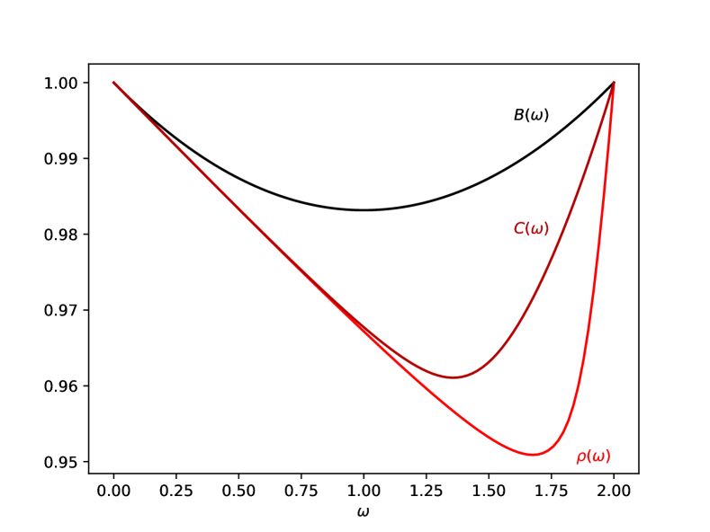
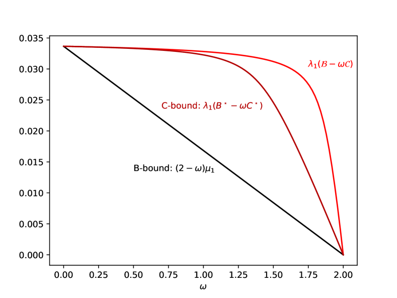
Figure 3: Upper bounds on the spectral radius of $\boldsymbol{\mathcal{A}}$ (left) correspond to lower bounds on the spectral gap of $\boldsymbol{\mathcal{B}}-\omega\boldsymbol{\mathcal{C}}$ (right).

Lemma 3 (The B-bound).

$\lambda_{i}(\boldsymbol{\mathcal{B}}-\omega\boldsymbol{\mathcal{C}})\geq(1-\omega/2)\lambda_{i}(\boldsymbol{\mathcal{B}})$

Proof.

Since $\boldsymbol{\mathcal{B}}\succcurlyeq 2\boldsymbol{\mathcal{C}}$, we have $\boldsymbol{\mathcal{B}}-\omega\boldsymbol{\mathcal{C}}\succcurlyeq\boldsymbol{\mathcal{B}}-\omega/2\boldsymbol{\mathcal{B}}=(1-\omega/2)\boldsymbol{\mathcal{B}}$. The Loewner order implies the order on the corresponding eigenvalues. ∎

This lemma re-establishes the B-bound in (5) since $\lambda_{\max}(\boldsymbol{\mathcal{A}}(\omega))=1-\omega\lambda_{1}(\boldsymbol{\mathcal{B}}-\omega\boldsymbol{\mathcal{C}})\geq 1-\omega(1-\omega/2)\lambda_{1}(\boldsymbol{\mathcal{B}})=1-\omega(1-\omega/2)2\mu_{1}$.

Lemma 4 (Concavity and Convexity).

$\lambda_{1}(\boldsymbol{\mathcal{B}}-\omega\boldsymbol{\mathcal{C}})$ is a concave, and equivalently, $\lambda_{\max}(\boldsymbol{\mathcal{A}}(\omega))$ is a convex function of $\omega$.

Proof.

$\boldsymbol{\mathcal{B}}-\omega\boldsymbol{\mathcal{C}}$ is an affine function of $\omega$ and the smallest eigenvalue is a concave function of its input due to the min-max theorem. Hence the composition is concave. ∎

These lemmas establish that $\lambda_{\max}(\boldsymbol{\mathcal{A}}(\omega))$ is generally a hockey stick as depicted in Figure 2.

4.2 Spectral Gap

Our approach for an upper bound on the spectral radius of $\boldsymbol{\mathcal{A}}(\omega)$ is to derive a lower bound for the spectral gap (i.e., smallest eigenvalue) of $\boldsymbol{\mathcal{B}}-\omega\boldsymbol{\mathcal{C}}$. The standard approach for analyzing and bounding eigenvalues is based on perturbation theory. One can bound the deviation of eigenvalues of $\boldsymbol{\mathcal{B}}-\omega\boldsymbol{\mathcal{C}}$ from those of $\boldsymbol{\mathcal{B}}$ based on bounds on derivatives of this eigenvalue with regards to $\omega$. Bounds on derivatives can be obtained from analyzing Hadamard variation formulae as shown in (Tao and Vu, 2011). However, being a general approach, the resulting perturbation bounds lead to negligible improvements over the B-bound. We leverage the interaction between $\boldsymbol{\mathcal{B}}$ and $\boldsymbol{\mathcal{C}}$ to develop a geometric approach for the smallest eigenvalue problem. Using this geometric view we build a surrogate $\boldsymbol{\mathcal{C}}^{\star}$ to $\boldsymbol{\mathcal{C}}$ that allows for bounding $\lambda_{1}(\boldsymbol{\mathcal{B}}-\omega\boldsymbol{\mathcal{C}})$ by the C-bound as in (9).

Irreducibility of ${\boldsymbol{A}}$ guarantees that spectral radius of $\boldsymbol{\mathcal{A}}(\omega)$ is a simple eigenvalue due to the Perron-Frobenius theorem for positive linear maps (see Section 4.4). This means $\lambda_{1}(\boldsymbol{\mathcal{B}}-\omega\boldsymbol{\mathcal{C}})$ is also a simple eigenvalue and hence differentiable with respect to $\omega$. Since we will be focusing on the smallest eigenvalue and the corresponding eigenvector of $\boldsymbol{\mathcal{B}}-\omega\boldsymbol{\mathcal{C}}$, for convenience of notation, we define each as a function of $\omega$:

$$\lambda(\omega):=\lambda_{1}(\boldsymbol{\mathcal{B}}-\omega\boldsymbol{\mathcal{C}}),\quad{\rm and}\quad\boldsymbol{V}(\omega):=\boldsymbol{V}_{1}(\boldsymbol{\mathcal{B}}-\omega\boldsymbol{\mathcal{C}}).$$ (15)

In particular, we have $\lambda(0)=\lambda_{1}(\boldsymbol{\mathcal{B}})=2\mu_{1}$ and $\lambda(2)=\lambda_{1}(\boldsymbol{\mathcal{B}}-2\boldsymbol{\mathcal{C}})=0$ according to Lemma 1.

Here is where $\xi$, the last ingredient in (8), enters the picture:

Lemma 5 (Derivatives with respect to $\omega$).

$$\dot{\lambda}(0)=-\langle\boldsymbol{V}_{1}(\boldsymbol{\mathcal{B}}),\boldsymbol{\mathcal{C}}(\boldsymbol{V}_{1}(\boldsymbol{\mathcal{B}}))\rangle=-\xi\quad{\rm and}\quad\dot{\lambda}(2)=-\frac{1}{n}\operatorname{tr}{\operatorname{\mathbb{E}}\left[\boldsymbol{P}\right]}$$ (16)

Proof.

Hadamard’s first variation formula together with the definition of $\boldsymbol{\mathcal{C}}$ in (12) provide:

$$\dot{\lambda}(\omega) =-\langle\boldsymbol{V}(\omega),\boldsymbol{\mathcal{C}}(\boldsymbol{V}(\omega))\rangle=-\langle\boldsymbol{V}(\omega),\operatorname{\mathbb{E}}\left[\boldsymbol{P}\boldsymbol{V}(\omega)\boldsymbol{P}\right]\rangle=-\operatorname{\mathbb{E}}\left[\langle\boldsymbol{V}(\omega),\boldsymbol{P}\boldsymbol{V}(\omega)\boldsymbol{P}\rangle\right]$$

$$=-\operatorname{\mathbb{E}}\left[\operatorname{tr}{\left(\boldsymbol{V}(\omega)^{T}\boldsymbol{P}\boldsymbol{V}(\omega)\boldsymbol{P}\right)}\right]=-\operatorname{\mathbb{E}}\left[\operatorname{tr}{\left(\boldsymbol{V}(\omega)\boldsymbol{P}\boldsymbol{V}(\omega)\boldsymbol{P}\right)}\right]$$

As we are interested in $\omega\in[0,2]$ we consider the right derivative at $\omega=0$ and the left derivative at $\omega=2$. Since $\boldsymbol{V}(0)=\boldsymbol{V}_{1}(\boldsymbol{\mathcal{B}})={\bf u}_{1}{\bf u}_{1}^{T}$ we have

$$\dot{\lambda}(0) =-\operatorname{\mathbb{E}}\left[\operatorname{tr}{\left({\bf u}_{1}{\bf u}_{1}^{T}\boldsymbol{P}{\bf u}_{1}{\bf u}_{1}^{T}\boldsymbol{P}\right)}\right]=-\operatorname{\mathbb{E}}\left[\operatorname{tr}{\left({\bf u}_{1}^{T}\boldsymbol{P}{\bf u}_{1}{\bf u}_{1}^{T}\boldsymbol{P}{\bf u}_{1}\right)}\right]=-\operatorname{\mathbb{E}}\left[\left({\bf u}_{1}^{T}\boldsymbol{P}{\bf u}_{1}\right)^{2}\right]=-\xi$$

as defined in (8). Moreover, Lemma 1 shows that $\boldsymbol{V}(2)=\frac{1}{\sqrt{n}}\boldsymbol{I}$ that readily implies $\dot{\lambda}(2)=-\frac{1}{n}\operatorname{tr}{\operatorname{\mathbb{E}}\left[\boldsymbol{P}\right]}$. ∎

As a result, based on (14), we have $\dot{\lambda}_{\max}(\boldsymbol{\mathcal{A}}(\omega))|_{\omega=0}=-2\mu_{1}$, $\dot{\lambda}_{\max}(\boldsymbol{\mathcal{A}}(\omega))|_{\omega=2}=\frac{2}{n}\operatorname{tr}{\operatorname{\mathbb{E}}\left[\boldsymbol{P}\right]}$ and $\ddot{\lambda}_{\max}(\boldsymbol{\mathcal{A}}(\omega))|_{\omega=0}=\xi$. These provide lower bounds for $\lambda_{\max}(\boldsymbol{\mathcal{A}}(\omega))$ due to its convexity and upper bounds for $\lambda_{1}(\boldsymbol{\mathcal{B}}-\omega\boldsymbol{\mathcal{C}})=\lambda(\omega)$ due to its concavity. These can be observed in Figure 3.

Lemma 6 (Ingredients in (8) satisfy $\mu_{1}^{2}\leq\xi\leq\mu_{1}$).

Proof.

According to Lemma 1: $\boldsymbol{\mathcal{C}}\preccurlyeq\frac{1}{2}\boldsymbol{\mathcal{B}}$, which implies:

$$\xi=\langle\boldsymbol{V}_{1}(\boldsymbol{\mathcal{B}}),\boldsymbol{\mathcal{C}}(\boldsymbol{V}_{1}(\boldsymbol{\mathcal{B}}))\rangle\leq\langle\boldsymbol{V}_{1}(\boldsymbol{\mathcal{B}}),\frac{1}{2}\boldsymbol{\mathcal{B}}(\boldsymbol{V}_{1}(\boldsymbol{\mathcal{B}}))\rangle=\lambda_{2}(\boldsymbol{\mathcal{B}})/2=\mu_{1}.$$

Since $\xi=\operatorname{\mathbb{E}}\left[\left({\bf u}_{1}^{T}\boldsymbol{P}{\bf u}_{1}\right)^{2}\right]$ and $\mu_{1}=\operatorname{\mathbb{E}}\left[\left({\bf u}_{1}^{T}\boldsymbol{P}{\bf u}_{1}\right)\right]$, the Jensen’s inequality shows $\xi\geq\mu_{1}^{2}$. ∎

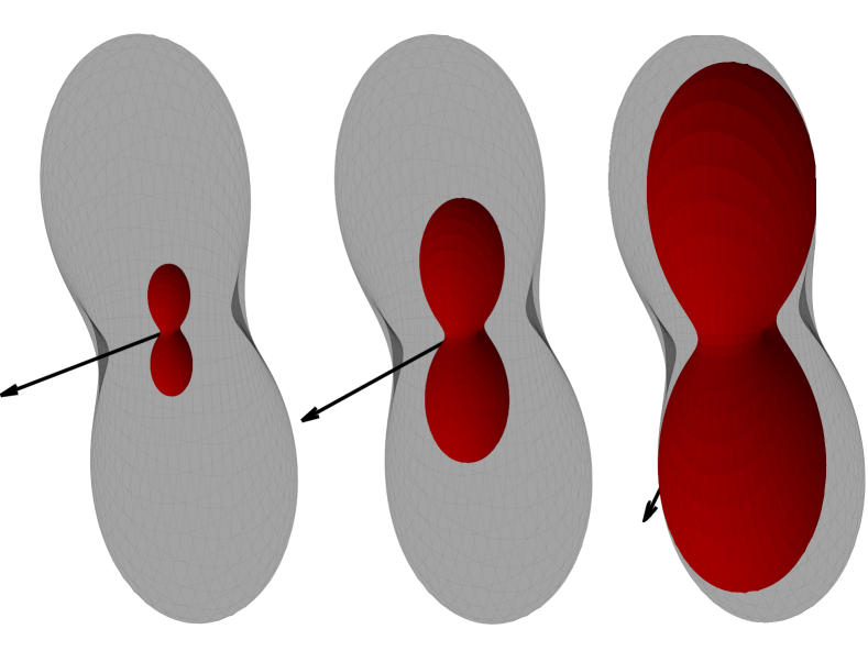
Figure 4: Geometric view of the smallest eigenvalue $\lambda_{1}(\boldsymbol{\mathcal{B}}-\omega\boldsymbol{\mathcal{C}})$ and the associated eigenvector $\boldsymbol{V}_{1}(\boldsymbol{\mathcal{B}}-\omega\boldsymbol{\mathcal{C}})$ along which the distance between $\boldsymbol{\mathcal{B}}$ and $\omega\boldsymbol{\mathcal{C}}$ is minimized. The eigenvector is shown for $\omega=1/2$ (left), $\omega=1$ (middle) and $\omega=2$ (right).

A geometric view

To build intuition, we visualize the quadratic forms for $\boldsymbol{\mathcal{B}}$ and $\omega\boldsymbol{\mathcal{C}}$ corresponding to a matrix ${\boldsymbol{A}}$ with $n=2$. Here the set of $2\times 2$ symmetric matrices, $\boldsymbol{V}$, can be visualized in 3 dimensions. Figure 4 shows height-fields over the sphere, probing $\boldsymbol{\mathcal{B}}$ and $\omega\boldsymbol{\mathcal{C}}$ along directions $\boldsymbol{V}$. Specifically the sphere $\lVert\boldsymbol{V}\rVert=1$ is transformed radially using the value $\langle\boldsymbol{V},\boldsymbol{\mathcal{B}}(\boldsymbol{V})\rangle:=\operatorname{tr}{\left(\boldsymbol{V}^{T}\boldsymbol{\mathcal{B}}(\boldsymbol{V})\right)}$ resulting in the (semi-transparent) black surface for $\boldsymbol{\mathcal{B}}$, and the red surface for $\omega\boldsymbol{\mathcal{C}}$. As $\omega$ increases from $0$ to $2$, the surface of $\omega\boldsymbol{\mathcal{C}}$ grows from the origin to a surface that touches $\boldsymbol{\mathcal{B}}$ at $\omega=2$. Lemma 1 shows $\boldsymbol{\mathcal{B}}\succcurlyeq 2\boldsymbol{\mathcal{C}}$ and the two surfaces actually meet at a single point along $\boldsymbol{I}$ making $\boldsymbol{\mathcal{B}}-2\boldsymbol{\mathcal{C}}$ semi-definite.

For every $\omega$, the smallest eigenvalue:

$$\lambda(\omega)=\min_{\langle\boldsymbol{V},\boldsymbol{V}\rangle=1}{\langle\boldsymbol{V},(\boldsymbol{\mathcal{B}}-\omega\boldsymbol{\mathcal{C}})(\boldsymbol{V})\rangle},$$ (17)

corresponds to an eigenvector $\boldsymbol{V}(\omega)$ along which the distance between the two surfaces is minimized. When $\omega=0$, $\boldsymbol{V}(0)=\boldsymbol{V}_{1}(\boldsymbol{\mathcal{B}})={\bf u}_{1}{\bf u}_{1}^{T}$ is the minimizer along with the minimum distance given by eigenvalue $\lambda(0)=\lambda_{1}(\boldsymbol{\mathcal{B}})=2\mu_{1}$ from the quantities discussed in (8). As $\omega$ increases, $\omega\boldsymbol{\mathcal{C}}$ grows inside $\boldsymbol{\mathcal{B}}$ and the eigenvector moves from $\boldsymbol{V}_{1}(\boldsymbol{\mathcal{B}})$ towards $\boldsymbol{V}_{1}(\boldsymbol{\mathcal{B}}-2\boldsymbol{\mathcal{C}})=\frac{1}{\sqrt{n}}\boldsymbol{I}$ while the eigenvalue drops from $2\mu_{1}$ to $0$. Figure 4 shows the eigenvector for $\omega=1/2$ (left), $\omega=1$ (middle) and $\omega=2$ (right).

4.3 The C-Bound

We remind the reader that we shall build a surrogate $\boldsymbol{\mathcal{C}}^{\star}$ to $\boldsymbol{\mathcal{C}}$ that allows for bounding $\lambda(\omega)=\lambda_{1}(\boldsymbol{\mathcal{B}}-\omega\boldsymbol{\mathcal{C}})$ by the C-bound as in (9). To do so we gather the properties that has been established about $\boldsymbol{\mathcal{C}}$:

Properties 2.

[Facts about $\boldsymbol{\mathcal{C}}$]

• Is positive semi-definite, $\boldsymbol{\mathcal{C}}\succcurlyeq\boldsymbol{0}$.

• Obeys the Loewner ordering with respect to $\boldsymbol{\mathcal{B}}$ specified as ${\boldsymbol{\mathcal{C}}}\preccurlyeq\boldsymbol{\mathcal{B}}/2$.

• Kisses $\boldsymbol{\mathcal{B}}/2$, i.e., $\boldsymbol{\mathcal{B}}/2-{\boldsymbol{\mathcal{C}}}$ is semi-definite.

• Satisfies $\langle\boldsymbol{V}_{1}(\boldsymbol{\mathcal{B}}),{\boldsymbol{\mathcal{C}}}(\boldsymbol{V}_{1}(\boldsymbol{\mathcal{B}}))\rangle=\xi$ as seen in Lemma 16.

We consider the set $\mathfrak{C}$ of all superoperators that satisfy these properties and define a partial ordering of its elements, denoted by $\uparrow$, with respect to $\boldsymbol{\mathcal{B}}$. For $\boldsymbol{\mathcal{C}}^{\prime},\boldsymbol{\mathcal{C}}^{\prime\prime}\in\mathfrak{C}$ we say $\boldsymbol{\mathcal{C}}^{\prime}$ eclipses $\boldsymbol{\mathcal{C}}^{\prime\prime}$ with respect to $\boldsymbol{\mathcal{B}}$:

$${\boldsymbol{\mathcal{C}}}^{\prime}\uparrow{\boldsymbol{\mathcal{C}}}^{\prime\prime}\iff\lambda_{1}(\boldsymbol{\mathcal{B}}-\omega{\boldsymbol{\mathcal{C}}}^{\prime})\leq\lambda_{1}(\boldsymbol{\mathcal{B}}-\omega{\boldsymbol{\mathcal{C}}}^{\prime\prime}),\forall\omega\in[0,2].$$ (18)

The importance of the eclipse relationship is that it is weaker than the Loewner order: ${\boldsymbol{\mathcal{C}}}^{\prime}\succcurlyeq{\boldsymbol{\mathcal{C}}}^{\prime\prime}$ implies ${\boldsymbol{\mathcal{C}}}^{\prime}\uparrow{\boldsymbol{\mathcal{C}}}^{\prime\prime}$, but not the other way around. The proof for the main theorem will identify a member $\boldsymbol{\mathcal{C}}^{\star}\in\mathfrak{C}$ that eclipses all elements of $\mathfrak{C}$, and therefore eclipses $\boldsymbol{\mathcal{C}}$.

For any $n\times n$ matrix $\boldsymbol{V}$ (unit length) orthogonal to $\boldsymbol{V}_{1}(\boldsymbol{\mathcal{B}})$ (i.e.,$\langle\boldsymbol{V}_{1}(\boldsymbol{\mathcal{B}}),\boldsymbol{V}\rangle=0$), we consider the two dimensional subspace spanned by $\boldsymbol{V}_{1}(\boldsymbol{\mathcal{B}})$ and $\boldsymbol{V}$ and define the superoperators:

$$\begin{split}\boldsymbol{\mathcal{C}}^{\star}_{\boldsymbol{V}}&:=\left(\sqrt{\gamma}\boldsymbol{V}+\sqrt{\xi}\boldsymbol{V}_{1}(\boldsymbol{\mathcal{B}})\right)\otimes\left(\sqrt{\gamma}\boldsymbol{V}+\sqrt{\xi}\boldsymbol{V}_{1}(\boldsymbol{\mathcal{B}})\right)\quad{\rm where}\quad\gamma:=\frac{\langle\boldsymbol{V},\boldsymbol{\mathcal{B}}(\boldsymbol{V})\rangle}{2}\left(1-\frac{\xi}{\mu_{1}}\right)\\ \boldsymbol{\mathcal{B}}_{\boldsymbol{V}}&:=\langle\boldsymbol{V},\boldsymbol{\mathcal{B}}(\boldsymbol{V})\rangle\boldsymbol{V}\otimes\boldsymbol{V}+2\mu_{1}\boldsymbol{V}_{1}(\boldsymbol{\mathcal{B}})\otimes\boldsymbol{V}_{1}(\boldsymbol{\mathcal{B}}).\end{split}$$ (19)

$\boldsymbol{\mathcal{B}}_{\boldsymbol{V}}$ is the restriction of $\boldsymbol{\mathcal{B}}$ to this subspace and as we will see below $\boldsymbol{\mathcal{C}}^{\star}_{\boldsymbol{V}}$ is the unique rank-1 superoperator in $\mathfrak{C}$ restricted to this subspace. Note that Lemma 6 implies $\gamma\geq 0$ since $\boldsymbol{\mathcal{B}}\succcurlyeq\boldsymbol{0}$. The introduced linear maps can be represented by these $2\times 2$ matrices:

$$\boldsymbol{B}_{\boldsymbol{V}}:=\begin{bmatrix}\langle\boldsymbol{V},\boldsymbol{\mathcal{B}}(\boldsymbol{V})\rangle&0\\ 0&2\mu_{1}\end{bmatrix}\quad{\rm and}\quad\boldsymbol{C}^{\star}_{\boldsymbol{V}}:=\begin{bmatrix}\sqrt{\gamma}\\ \sqrt{\xi}\end{bmatrix}\begin{bmatrix}\sqrt{\gamma}&\sqrt{\xi}\end{bmatrix}=\begin{bmatrix}\gamma&\sqrt{\gamma\xi}\\ \sqrt{\gamma\xi}&\xi\end{bmatrix}$$

in the basis of $\boldsymbol{V}$ and $\boldsymbol{V}_{1}(\boldsymbol{\mathcal{B}})$ and live in this subspace; formally, for any $n\times n$ matrix $\boldsymbol{V}^{\prime}$ orthogonal to $\boldsymbol{V}_{1}(\boldsymbol{\mathcal{B}})$ and $\boldsymbol{V}$, we have $\boldsymbol{\mathcal{C}}^{\star}_{\boldsymbol{V}}(\boldsymbol{V}^{\prime})=\boldsymbol{\mathcal{B}}_{\boldsymbol{V}}(\boldsymbol{V}^{\prime})=\boldsymbol{0}$.

Proposition 1 ($\boldsymbol{\mathcal{C}}^{\star}_{\boldsymbol{V}}\in\mathfrak{C}$).

Proof.

Positivity of $\boldsymbol{\mathcal{C}}^{\star}_{\boldsymbol{V}}$ follows from the definition (19). We have: $\langle\boldsymbol{V}_{1}(\boldsymbol{\mathcal{B}}),\boldsymbol{\mathcal{C}}^{\star}_{\boldsymbol{V}}(\boldsymbol{V}_{1}(\boldsymbol{\mathcal{B}}))\rangle=\xi$, since $\langle\boldsymbol{V},\boldsymbol{V}_{1}(\boldsymbol{\mathcal{B}})\rangle=0$. To show that $\boldsymbol{\mathcal{C}}^{\star}_{\boldsymbol{V}}$ kisses $\boldsymbol{\mathcal{B}}/2$, we use the restriction of $\boldsymbol{\mathcal{B}}$ to the subspace, namely $\boldsymbol{\mathcal{B}}_{\boldsymbol{V}}$. Then, we examine the matrix representations and, noting from (19) that $\langle\boldsymbol{V},\boldsymbol{\mathcal{B}}(\boldsymbol{V})\rangle=\frac{2\gamma\mu_{1}}{\mu_{1}-\xi}$ that:

$$\det\left(\boldsymbol{B}_{\boldsymbol{V}}/2-\boldsymbol{C}^{\star}_{\boldsymbol{V}}\right)=\begin{vmatrix}\frac{\gamma\mu_{1}}{\mu_{1}-\xi}-\gamma&-\sqrt{\gamma\xi}\\ -\sqrt{\gamma\xi}&\mu_{1}-\xi\end{vmatrix}=\begin{vmatrix}\frac{\gamma\xi}{\mu_{1}-\xi}&-\sqrt{\gamma\xi}\\ -\sqrt{\gamma\xi}&\mu_{1}-\xi\end{vmatrix}=0.$$

Showing one of the two eigenvalues is 0. The other eigenvalue can be obtained from the trace:

$$\operatorname{tr}{\left(\boldsymbol{B}_{\boldsymbol{V}}/2-\boldsymbol{C}^{\star}_{\boldsymbol{V}}\right)}=\frac{\gamma\xi}{\mu_{1}-\xi}+(\mu_{1}-\xi)\geq 0,$$

due to Lemma 6. This means $\boldsymbol{C}^{\star}_{\boldsymbol{V}}\preccurlyeq\boldsymbol{B}_{\boldsymbol{V}}/2$ implying $\boldsymbol{\mathcal{C}}^{\star}_{\boldsymbol{V}}\preccurlyeq\boldsymbol{\mathcal{B}}_{\boldsymbol{V}}/2$. ∎

Recall from Properties 1 that $\lambda_{2}(\boldsymbol{\mathcal{B}})=\mu_{1}+\mu_{2}$ is a repeated eigenvalue with the corresponding eigenspace we denote by $\boldsymbol{V}_{2}(\boldsymbol{\mathcal{B}})$. The surrogate $\boldsymbol{\mathcal{C}}^{\star}$ is defined by picking $\boldsymbol{V}$ from this subspace:

$$\boldsymbol{\mathcal{C}}^{\star}:=\boldsymbol{\mathcal{C}}^{\star}_{\boldsymbol{V}^{\star}}\quad{\rm with}\quad\boldsymbol{V}^{\star}\in\boldsymbol{V}_{2}(\boldsymbol{\mathcal{B}}),\quad{\rm and}\quad\gamma^{\star}:=\frac{\mu_{1}+\mu_{2}}{2}\left(1-\frac{\xi}{\mu_{1}}\right).$$ (20)

This choice of surrogate corresponds to the C-bound with the $2\times 2$ matrices $\boldsymbol{B}^{\star}$ and $\boldsymbol{C}^{\star}$ described in (9). The strategy to prove the main result is to establish $\boldsymbol{\mathcal{C}}^{\star}\uparrow{\boldsymbol{\mathcal{C}}}$ by showing that it eclipses all elements of $\mathfrak{C}$. To that end:

1. We first show that for any two dimensional subspace spanned by $\boldsymbol{V}_{1}(\boldsymbol{\mathcal{B}})$ and an $n\times n$ matrix $\boldsymbol{V}$ orthogonal to it (i.e.,$\langle\boldsymbol{V}_{1}(\boldsymbol{\mathcal{B}}),\boldsymbol{V}\rangle=0$), $\boldsymbol{\mathcal{C}}^{\star}_{\boldsymbol{V}}$ eclipses any other element of $\mathfrak{C}$ living in that subspace.

2. We then show that $\boldsymbol{\mathcal{C}}^{\star}\uparrow\boldsymbol{\mathcal{C}}^{\star}_{\boldsymbol{V}}$ for any $\boldsymbol{V}$ that is orthogonal to $\boldsymbol{V}_{1}(\boldsymbol{\mathcal{B}})$.

3. The proof is completed by showing that if an element of $\mathfrak{C}$ were to violate the C-bound, there has to exist a $\boldsymbol{V}$ orthogonal to $\boldsymbol{V}_{1}(\boldsymbol{\mathcal{B}})$ and an element of $\mathfrak{C}$ that lives in the two dimensional subspace spanned by $\boldsymbol{V}_{1}(\boldsymbol{\mathcal{B}})$ and $\boldsymbol{V}$ that violates the eclipse relationship in part 1 and 2 above.

Proposition 2.

For any two dimensional subspace spanned by $\boldsymbol{V}_{1}(\boldsymbol{\mathcal{B}})$ and some $\boldsymbol{V}$ orthogonal to $\boldsymbol{V}_{1}(\boldsymbol{\mathcal{B}})$, the rank-1 superoperator $\boldsymbol{\mathcal{C}}^{\star}_{\boldsymbol{V}}$, defined in (19), eclipses any $\boldsymbol{\mathcal{C}}_{\boldsymbol{V}}\in\mathfrak{C}$ living in this subspace.

Proof.

In this subspace, $\boldsymbol{\mathcal{C}}_{\boldsymbol{V}}\in\mathfrak{C}$ is a general superoperator and $\boldsymbol{\mathcal{C}}^{\star}_{\boldsymbol{V}}$ is the unique rank-1 superoperator satisfying Properties 2. Let $\pi:=\frac{1}{2}\langle\boldsymbol{V},\boldsymbol{\mathcal{B}}(\boldsymbol{V})\rangle$. For a $\sigma\geq 0$, the corresponding superoperator, $\boldsymbol{\mathcal{C}}_{\boldsymbol{V}}$, can be viewed in the $2\times 2$ representations, as:

$$\boldsymbol{B}_{\boldsymbol{V}}=\begin{bmatrix}2\pi&0\\ 0&2\mu_{1}\end{bmatrix}\quad{\rm and}\quad\boldsymbol{C}_{\boldsymbol{V}}=\begin{bmatrix}\sqrt{\alpha}\\ \sqrt{\xi}\end{bmatrix}\begin{bmatrix}\sqrt{\alpha}&\sqrt{\xi}\end{bmatrix}+\begin{bmatrix}\sigma&0\\ 0&0\end{bmatrix}=\begin{bmatrix}\alpha+\sigma&\sqrt{\alpha\xi}\\ \sqrt{\alpha\xi}&\xi\end{bmatrix}.$$

We note that when $\sigma=0$, $\boldsymbol{\mathcal{C}}_{\boldsymbol{V}}=\boldsymbol{\mathcal{C}}^{\star}_{\boldsymbol{V}}$; furthermore, any rank-2 symmetric positive semi-definite matrix, $\boldsymbol{C}_{\boldsymbol{V}}$, representing a $\boldsymbol{\mathcal{C}}_{\boldsymbol{V}}$ that satisfies $\langle\boldsymbol{V}_{1}(\boldsymbol{\mathcal{B}}),\boldsymbol{\mathcal{C}}_{\boldsymbol{V}}(\boldsymbol{V}_{1}(\boldsymbol{\mathcal{B}}))\rangle=\boldsymbol{C}_{\boldsymbol{V}}[1,1]=\xi$ can be represented in this form. We show that for any fixed $\omega$, the smaller eigenvalue of $\boldsymbol{B}_{\boldsymbol{V}}-\omega\boldsymbol{C}_{\boldsymbol{V}}$, as a function of $\sigma$, increases as $\sigma$ increases by showing that its derivative with respect to $\sigma$ is non-negative.

Since $\boldsymbol{\mathcal{C}}_{\boldsymbol{V}}\in\mathfrak{C}$, we have $\det\left(\boldsymbol{B}_{\boldsymbol{V}}/2-\boldsymbol{C}_{\boldsymbol{V}}\right)=0$. Just like in Proposition 1:

$$\det\left(\boldsymbol{B}_{\boldsymbol{V}}/2-\boldsymbol{C}_{\boldsymbol{V}}\right)=\begin{vmatrix}\pi-\alpha-\sigma&-\sqrt{\alpha\xi}\\ -\sqrt{\alpha\xi}&\mu_{1}-\xi\end{vmatrix}=(\pi-\alpha-\sigma)(\mu_{1}-\xi)-\alpha\xi=0.$$

This poses the first constraint relating $\sigma$ and $\alpha$:

$$\alpha=(\pi-\sigma)\left(1-\frac{\xi}{\mu_{1}}\right).$$ (21)

For any relaxation value $\omega$, we consider the smaller eigenvalue of $\boldsymbol{B}_{\boldsymbol{V}}-\omega\boldsymbol{C}_{\boldsymbol{V}}$:

$$\lambda_{1}(\boldsymbol{B}_{\boldsymbol{V}}-\omega\boldsymbol{C}_{\boldsymbol{V}})=\lambda_{1}\left(\begin{bmatrix}2\pi-\omega(\alpha+\sigma)&-\omega\sqrt{\alpha\xi}\\ -\omega\sqrt{\alpha\xi}&2\mu_{1}-\omega\xi\end{bmatrix}\right).$$

Since eigenvalues of a $2\times 2$ symmetric matrix $\boldsymbol{M}$ are given by $\left(\operatorname{tr}\boldsymbol{M}/2\right)\pm\sqrt{\left(\operatorname{tr}\boldsymbol{M}/2\right)^{2}-\det\boldsymbol{M}}$, we introduce these quantities as:

$$X :=\operatorname{tr}{\left(\boldsymbol{B}_{\boldsymbol{V}}-\omega\boldsymbol{C}_{\boldsymbol{V}}\right)}/2=\pi+\mu_{1}-\frac{1}{2}\omega(\alpha+\sigma+\xi)$$

$$Y :=\det{\left(\boldsymbol{B}_{\boldsymbol{V}}-\omega\boldsymbol{C}_{\boldsymbol{V}}\right)}=2\pi\mu_{1}(2-\omega)-\omega(2-\omega)\sigma\xi.$$

The last equality follows from the constraint (21). The smaller eigenvalue of $\boldsymbol{B}_{\boldsymbol{V}}-\omega\boldsymbol{C}_{\boldsymbol{V}}$ is given by $\lambda_{1}(\boldsymbol{B}_{\boldsymbol{V}}-\omega\boldsymbol{C}_{\boldsymbol{V}})=X-\sqrt{X^{2}-Y}$.

Recall that when $\sigma=0$, $\boldsymbol{\mathcal{C}}^{\star}_{\boldsymbol{V}}=\boldsymbol{\mathcal{C}}_{\boldsymbol{V}}$. In order to prove $\boldsymbol{\mathcal{C}}^{\star}_{\boldsymbol{V}}\uparrow\boldsymbol{\mathcal{C}}_{\boldsymbol{V}}$ we establish that this smaller eigenvalue, for any $\omega\in[0,2]$, increases with $\sigma$. We show this by taking the derivative with respect to $\sigma$:

$$\frac{\partial\lambda_{1}(\boldsymbol{B}_{\boldsymbol{V}}-\omega\boldsymbol{C}_{\boldsymbol{V}})}{\partial\sigma}=\frac{\partial X}{\partial\sigma}-\frac{1}{2\sqrt{X^{2}-Y}}\left(2X\frac{\partial X}{\partial\sigma}-\frac{\partial Y}{\partial\sigma}\right).$$

By using the constraint in (21), we have $\frac{\partial X}{\partial\sigma}=-\frac{\omega\xi}{2\mu_{1}}$. Similarly, $\frac{\partial Y}{\partial\sigma}=\omega(\omega-2)\xi$ that yields:

$$\frac{\partial\lambda_{1}(\boldsymbol{B}_{\boldsymbol{V}}-\omega\boldsymbol{C}_{\boldsymbol{V}})}{\partial\sigma}=-\frac{\omega\xi}{2\mu_{1}}-\frac{1}{2\sqrt{X^{2}-Y}}\left(-2X\frac{\omega\xi}{2\mu_{1}}-\omega(\omega-2)\xi\right)=\frac{\omega\xi}{2\mu_{1}}\left(\frac{X-(2-\omega)\mu_{1}}{\sqrt{X^{2}-Y}}-1\right).$$

Since $\boldsymbol{\mathcal{C}}_{\boldsymbol{V}}\in\mathfrak{C}$, we have $\boldsymbol{C}_{\boldsymbol{V}}\preccurlyeq\boldsymbol{B}_{\boldsymbol{V}}/2$ and $\lambda_{1}(\boldsymbol{B}_{\boldsymbol{V}}-\omega\boldsymbol{C}_{\boldsymbol{V}})\geq\lambda_{1}(\boldsymbol{B}_{\boldsymbol{V}}-\omega\boldsymbol{B}_{\boldsymbol{V}}/2)=(2-\omega)\mu_{1}$. Since $X=\operatorname{tr}{\left(\boldsymbol{B}_{\boldsymbol{V}}-\omega\boldsymbol{C}_{\boldsymbol{V}}\right)}/2$ is the average of its two eigenvalues and $(2-\omega)\mu_{1}$ is a lower bound for the smaller eigenvalue, we have $X-(2-\omega)\mu_{1}\geq 0$. To show $X-(2-\omega)\mu_{1}\geq\sqrt{X^{2}-Y}$ we take the square and consider the difference:

$$(X-(2-\omega)\mu_{1})^{2}-X^{2}+Y =(2-\omega)^{2}\mu_{1}^{2}-2(2-\omega)\mu_{1}X+Y$$

$$=(2-\omega)\mu_{1}\left[(2-\omega)\mu_{1}-2\pi-2\mu_{1}+\omega(\alpha+\sigma+\xi)+2\pi-\omega\sigma\frac{\xi}{\mu_{1}}\right]$$

$$=\omega(2-\omega)\mu_{1}\left[\alpha-(\mu_{1}-\xi)+\sigma\left(1-\frac{\xi}{\mu_{1}}\right)\right]$$

$$=\omega(2-\omega)\mu_{1}\left[(\pi-\sigma)\left(1-\frac{\xi}{\mu_{1}}\right)-(\mu_{1}-\xi)+\sigma\left(1-\frac{\xi}{\mu_{1}}\right)\right]$$

$$=\omega(2-\omega)\mu_{1}\left[\pi\left(1-\frac{\xi}{\mu_{1}}\right)-(\mu_{1}-\xi)\right]$$

$$=\omega(2-\omega)(\mu_{1}-\xi)(\pi-\mu_{1})\geq 0.$$

Lemma 6 shows $\xi\leq\mu_{1}$ and $\mu_{1}\leq\pi$ since $2\mu_{1}=\langle\boldsymbol{V}_{1}(\boldsymbol{\mathcal{B}}),\boldsymbol{\mathcal{B}}(\boldsymbol{V}_{1}(\boldsymbol{\mathcal{B}}))\rangle\leq\langle\boldsymbol{V},\boldsymbol{\mathcal{B}}(\boldsymbol{V})\rangle=2\pi$ as $\boldsymbol{V}$ is orthogonal to $\boldsymbol{V}_{1}(\boldsymbol{\mathcal{B}})$. This shows that for any $\omega$ the derivative ${\partial\lambda_{1}(\boldsymbol{B}_{\boldsymbol{V}}-\omega\boldsymbol{C}_{\boldsymbol{V}})}/{\partial\sigma}\geq 0$. Since $\boldsymbol{\mathcal{C}}_{\boldsymbol{V}}=\boldsymbol{\mathcal{C}}^{\star}_{\boldsymbol{V}}$ when $\sigma=0$, $\boldsymbol{\mathcal{C}}^{\star}_{\boldsymbol{V}}\uparrow\boldsymbol{\mathcal{C}}_{\boldsymbol{V}}$ for $\sigma\geq 0$. ∎

This proposition establishes that the rank-1 superoperator $\boldsymbol{\mathcal{C}}^{\star}_{\boldsymbol{V}}$, corresponding to $\sigma=0$, is to be studied.

Proposition 3.

The surrogate $\boldsymbol{\mathcal{C}}^{\star}$ defined in (20), eclipses any other surrogate $\boldsymbol{\mathcal{C}}^{\star}_{\boldsymbol{V}}$ defined in (19) for a $\boldsymbol{V}$ that is orthogonal to $\boldsymbol{V}_{1}(\boldsymbol{\mathcal{B}})$.

Proof.

We recall the $2\times 2$ matrix representations $\boldsymbol{B}_{\boldsymbol{V}}$ and $\boldsymbol{C}^{\star}_{\boldsymbol{V}}$ from (19) and denote $\pi:=\frac{1}{2}\langle\boldsymbol{V},\boldsymbol{\mathcal{B}}(\boldsymbol{V})\rangle$. We note that if $\boldsymbol{V}\in\boldsymbol{V}_{2}(\boldsymbol{\mathcal{B}})$ then $\boldsymbol{\mathcal{C}}^{\star}_{\boldsymbol{V}}=\boldsymbol{\mathcal{C}}^{\star}$ where $\pi=\frac{1}{2}\lambda_{2}(\boldsymbol{\mathcal{B}})$ is minimized due to the min-max theorem. To show $\boldsymbol{\mathcal{C}}^{\star}\uparrow\boldsymbol{\mathcal{C}}^{\star}_{\boldsymbol{V}}$ we once again show that for any fixed $\omega$, the smaller eigenvalue of $\boldsymbol{B}_{\boldsymbol{V}}-\omega\boldsymbol{C}^{\star}_{\boldsymbol{V}}$ increases when $\pi$ increases away from its minimum for a changing $\boldsymbol{V}$ that is orthogonal to $\boldsymbol{V}_{1}(\boldsymbol{\mathcal{B}})$. We take the same approach, as in the previous Proposition, by showing that the derivative with respect to $\pi$ is non-negative. The smaller eigenvalue of $\boldsymbol{B}_{\boldsymbol{V}}-\omega\boldsymbol{C}_{\boldsymbol{V}}$ as a function of $\pi$ is:

$$\lambda_{1}(\boldsymbol{B}_{\boldsymbol{V}}-\omega\boldsymbol{C}_{\boldsymbol{V}})=\lambda_{1}\left(\begin{bmatrix}2\pi&0\\ 0&2\mu_{1}\end{bmatrix}-\omega\begin{bmatrix}\gamma&\sqrt{\gamma\xi}\\ \sqrt{\gamma\xi}&\xi\end{bmatrix}\right)=\lambda_{1}\left(\begin{bmatrix}2\pi-\omega\gamma&-\omega\sqrt{\gamma\xi}\\ -\omega\sqrt{\gamma\xi}&2\mu_{1}-\omega\xi\end{bmatrix}\right),$$

recalling from (21) and (19) that $\gamma=\pi\left(1-\xi/\mu_{1}\right)$. As before, eigenvalues of this $2\times 2$ symmetric matrix can be derived from its trace and determinant:

$$X :=\operatorname{tr}{\left(\boldsymbol{B}_{\boldsymbol{V}}-\omega\boldsymbol{C}_{\boldsymbol{V}}\right)}/2=\pi+\mu_{1}-\frac{1}{2}\omega(\gamma+\xi)=\pi\left(1-\frac{1}{2}\omega\left(1-\frac{\xi}{\mu_{1}}\right)\right)+\mu_{1}-\frac{\omega\xi}{2}$$

$$Y :=\det{\left(\boldsymbol{B}_{\boldsymbol{V}}-\omega\boldsymbol{C}_{\boldsymbol{V}}\right)}=2\pi\mu_{1}(2-\omega).$$

The smaller eigenvalue of $\boldsymbol{B}_{\boldsymbol{V}}-\omega\boldsymbol{C}_{\boldsymbol{V}}$ is given by $\lambda_{1}(\boldsymbol{B}_{\boldsymbol{V}}-\omega\boldsymbol{C}_{\boldsymbol{V}})=X-\sqrt{X^{2}-Y}$ whose derivative with respect to $\pi$, using $Z:=\partial X/\partial\pi=1-\frac{1}{2}\omega(1-\xi/\mu_{1})$ and $\partial Y/\partial\pi=2\mu_{1}(2-\omega)$ is:

$$\frac{\partial\lambda_{1}(\boldsymbol{B}_{\boldsymbol{V}}-\omega\boldsymbol{C}_{\boldsymbol{V}})}{\partial\pi}=Z-\frac{XZ-\mu_{1}(2-\omega)}{\sqrt{X^{2}-Y}}.$$

We need to prove that $\partial\lambda_{1}(\boldsymbol{B}_{\boldsymbol{V}}-\omega\boldsymbol{C}_{\boldsymbol{V}})/{\partial\pi}\geq 0$, alternatively: $Z\sqrt{X^{2}-Y}\geq XZ-\mu_{1}(2-\omega)$. Note that from $\omega\in[0,2]$ and Lemma 6, we have $Z\geq 0$ and if $XZ-\mu_{1}(2-\omega)\leq 0$ the positivity is trivially established. With the assumption that the latter is positive, we square both sides:

$$Z^{2}(X^{2}-Y) \geq X^{2}Z^{2}+\mu_{1}^{2}(2-\omega)^{2}-2\mu_{1}(2-\omega)XZ\quad{\rm or}$$

$$2\mu_{1}(2-\omega)XZ \geq\mu_{1}^{2}(2-\omega)^{2}+Z^{2}Y.$$

Plugging in the value of $Y$, we need to show:

$$2XZ\geq\mu_{1}(2-\omega)+2\pi Z^{2}.$$

Noting that $X=\pi Z+\mu_{1}-\omega\xi/2$, the inequality becomes:

$$2\mu_{1}Z-\omega\xi Z\geq\mu_{1}(2-\omega).$$

Bringing in $Z$ results in the inequality:

$$\frac{\omega^{2}\xi}{2}\left(1-\frac{\xi}{\mu_{1}}\right)\geq 0,$$

which holds because of Lemma 6. ∎

This proposition establishes that the rank-1 superoperator $\boldsymbol{\mathcal{C}}^{\star}$, corresponding to $\pi=\frac{1}{2}\lambda_{2}(\boldsymbol{\mathcal{B}})=\frac{1}{2}(\mu_{1}+\mu_{2})$, eclipses elements of $\mathfrak{C}$ that live in any two dimensional subspace spanned by $\boldsymbol{V}_{1}(\boldsymbol{\mathcal{B}})$ and any matrix $\boldsymbol{V}$ orthogonal to it.

Theorem 2 ($\boldsymbol{\mathcal{C}}^{\star}\uparrow\boldsymbol{\mathcal{C}}$).

The $\boldsymbol{\mathcal{C}}^{\star}$, defined in (20), eclipses all elements of $\mathfrak{C}$, hence eclipsing $\boldsymbol{\mathcal{C}}$ defined in (12) for the problem ${\boldsymbol{A}}{{\bf x}}={{\bf b}}$.

Proof.

The proof is by contradiction. Let $\boldsymbol{\mathcal{C}}^{\prime}\in\mathfrak{C}$ that violates the eclipse relationship with $\boldsymbol{\mathcal{C}}^{\star}$. Then according to (18), there exists an $\omega_{0}\in[0,2]$ for which we have the strict inequality:

$$\lambda_{1}(\boldsymbol{\mathcal{B}}-\omega_{0}{\boldsymbol{\mathcal{C}}}^{\prime})<\lambda_{1}(\boldsymbol{\mathcal{B}}-\omega_{0}{\boldsymbol{\mathcal{C}}}^{\star}).$$

For this particular $\omega_{0}$, we consider the corresponding eigenvector: $\boldsymbol{V}_{1}(\boldsymbol{\mathcal{B}}-\omega_{0}\boldsymbol{\mathcal{C}}^{\prime})$, and denote its component orthogonal to $\boldsymbol{V}_{1}(\boldsymbol{\mathcal{B}})$ by $\boldsymbol{V}$. Note that $\boldsymbol{V}$ can not be zero. Otherwise, $\boldsymbol{V}_{1}(\boldsymbol{\mathcal{B}}-\omega_{0}\boldsymbol{\mathcal{C}}^{\prime})=\boldsymbol{V}_{1}(\boldsymbol{\mathcal{B}})$; therefore, $\lambda_{1}(\boldsymbol{\mathcal{B}}-\omega_{0}\boldsymbol{\mathcal{C}}^{\prime})=\langle\boldsymbol{V}_{1}(\boldsymbol{\mathcal{B}}),\left(\boldsymbol{\mathcal{B}}-\omega_{0}\boldsymbol{\mathcal{C}}^{\prime}\right)(\boldsymbol{V}_{1}(\boldsymbol{\mathcal{B}}))\rangle=2\mu_{1}-\omega_{0}\xi$ since $\boldsymbol{\mathcal{C}}^{\prime}\in\mathfrak{C}$. So the strict inequality is asserting that $2\mu_{1}-\omega_{0}\xi<\lambda_{1}(\boldsymbol{\mathcal{B}}-\omega_{0}\boldsymbol{\mathcal{C}}^{\star})$. However, the arguments in Lemmas 4 and 16, that apply to $\boldsymbol{\mathcal{C}}^{\star}$ (since $\boldsymbol{\mathcal{C}}^{\star}\in\mathfrak{C}$), show that $\lambda_{1}(\boldsymbol{\mathcal{B}}-\omega\boldsymbol{\mathcal{C}}^{\star})$ is a concave function of $\omega$ and that the linear function $2\mu_{1}-\omega\xi$ is an upper bound for it. This violates the strict inequality in: $\lambda_{1}(\boldsymbol{\mathcal{B}}-\omega_{0}\boldsymbol{\mathcal{C}}^{\prime})=2\mu_{1}-\omega_{0}\xi<\lambda_{1}(\boldsymbol{\mathcal{B}}-\omega_{0}\boldsymbol{\mathcal{C}}^{\star})\leq 2\mu_{1}-\omega_{0}\xi$.

Let $S$ denote the two dimensional subspace spanned by $\boldsymbol{V}_{1}(\boldsymbol{\mathcal{B}})$ and $\boldsymbol{V}$ and $\boldsymbol{\mathcal{C}}^{\prime}_{S}$ denote the restriction of $\boldsymbol{\mathcal{C}}^{\prime}$ to this subspace (i.e., $\boldsymbol{\mathcal{C}}^{\prime}_{S}$ agrees with $\boldsymbol{\mathcal{C}}^{\prime}$ for any vector in this subspace and assigns $\boldsymbol{0}$ to any element outside). Also $\boldsymbol{V}_{1}(\boldsymbol{\mathcal{B}}-\omega_{0}\boldsymbol{\mathcal{C}}^{\prime})\in S$ by the definition of $\boldsymbol{V}$ and $\lambda_{1}(\boldsymbol{\mathcal{B}}-\omega_{0}\boldsymbol{\mathcal{C}}^{\prime}_{S})=\lambda_{1}(\boldsymbol{\mathcal{B}}-\omega_{0}\boldsymbol{\mathcal{C}}^{\prime})$.

Since $\boldsymbol{\mathcal{C}}^{\prime}\in\mathfrak{C}$, its restriction to $S$ satisfies $\langle\boldsymbol{V}_{1}(\boldsymbol{\mathcal{B}}),\boldsymbol{\mathcal{C}}^{\prime}_{S}(\boldsymbol{V}_{1}(\boldsymbol{\mathcal{B}}))\rangle=\xi$. Also, $\boldsymbol{\mathcal{C}}^{\prime}_{S}\preccurlyeq\boldsymbol{\mathcal{B}}/2$ since $\boldsymbol{\mathcal{C}}^{\prime}\preccurlyeq\boldsymbol{\mathcal{B}}/2$. To satisfy the kissing constraint in Properties 2, we can add a component along $\boldsymbol{V}$: $\boldsymbol{\mathcal{C}}^{\prime\prime}_{S}:=\boldsymbol{\mathcal{C}}^{\prime}_{S}+\delta\boldsymbol{V}\otimes\boldsymbol{V}\in\mathfrak{C}$ for some $\delta\geq 0$. Since $\boldsymbol{\mathcal{C}}^{\prime\prime}_{S}\succcurlyeq\boldsymbol{\mathcal{C}}^{\prime}_{S}$ we have $\lambda_{1}(\boldsymbol{\mathcal{B}}-\omega_{0}\boldsymbol{\mathcal{C}}^{\prime\prime}_{S})\leq\lambda_{1}(\boldsymbol{\mathcal{B}}-\omega_{0}\boldsymbol{\mathcal{C}}^{\prime}_{S})$. Proposition 3 establishes $\boldsymbol{\mathcal{C}}^{\star}\uparrow\boldsymbol{\mathcal{C}}^{\prime\prime}_{S}$, a relationship that applies to all $\omega\in[0,2]$, that guarantees:

$$\lambda_{1}(\boldsymbol{\mathcal{B}}-\omega_{0}\boldsymbol{\mathcal{C}}^{\star})\leq\lambda_{1}(\boldsymbol{\mathcal{B}}-\omega_{0}\boldsymbol{\mathcal{C}}^{\prime\prime}_{S})\leq\lambda_{1}(\boldsymbol{\mathcal{B}}-\omega_{0}\boldsymbol{\mathcal{C}}^{\prime}_{S}).$$

This is in contradiction with the strict inequality $\lambda_{1}(\boldsymbol{\mathcal{B}}-\omega_{0}\boldsymbol{\mathcal{C}}^{\star})>\lambda_{1}(\boldsymbol{\mathcal{B}}-\omega_{0}\boldsymbol{\mathcal{C}}^{\prime})$. ∎

Proof of Theorem 1.

Theorem 2 implies $\lambda_{1}(\boldsymbol{B}^{\star}-\omega\boldsymbol{C}^{\star})=\lambda_{1}(\boldsymbol{\mathcal{B}}-\omega\boldsymbol{\mathcal{C}}^{\star})\leq\lambda_{1}(\boldsymbol{\mathcal{B}}-\omega\boldsymbol{\mathcal{C}})$ for $\omega\in[0,2]$ that establishes $C(\omega)\geq\lambda_{\max}(\boldsymbol{\mathcal{A}}(\omega))$ based on (14). The covariance $\boldsymbol{\Sigma}_{k}$ converges to $\boldsymbol{0}$ according to the rate given by $\lambda_{\max}(\boldsymbol{\mathcal{A}}(\omega))$ and the expected error at each step is the trace of $\boldsymbol{\Sigma}_{k}$: $\operatorname{\mathbb{E}}\left[\lVert\boldsymbol{\varepsilon}_{k}\rVert^{2}\right]=\operatorname{tr}{\boldsymbol{\Sigma}_{k}}$. When $i$ is drawn independently and identically distributed at each step of (1), the geometric rate of convergence is bound by $C(\omega)$ for every $\omega\in[0,2]$. ∎

4.4 Perron-Frobenius Theory For Positive Linear Maps

The superoperator $\boldsymbol{\mathcal{A}}$ defined in (7) plays the role of the iteration matrix — whose spectrum provides convergence analysis in classical iterative methods (Saad, 2003) — for randomized iterations. In this section we discuss the theoretical foundations that provide necessary properties on the spectrum of $\boldsymbol{\mathcal{A}}$ in the covariance analysis we have seen.

Recall the superoperator $\boldsymbol{\mathcal{A}}$, for a fixed $\omega$, denotes a linear map over the space of $n\times n$ matrices as:

$$\boldsymbol{\mathcal{A}}(\boldsymbol{X})=\frac{1}{m}\sum_{i=1}^{m}{(\boldsymbol{I}-\omega\boldsymbol{P}_{i})\boldsymbol{X}(\boldsymbol{I}-\omega\boldsymbol{P}_{i})}.$$

Since orthogonal projection is a symmetric operator, for any symmetric positive semi-definite matrix $\boldsymbol{X}$ the operation $(\boldsymbol{I}-\omega\boldsymbol{P}_{i})\boldsymbol{X}(\boldsymbol{I}-\omega\boldsymbol{P}_{i})$ preserves its positivity (Bhatia, 2009). Hence the superoperator $\boldsymbol{\mathcal{A}}$ is a positive linear map, leaving the cone of symmetric positive semi-definite matrices invariant.

The spectra of positive linear maps on general (noncommutative) matrix algebras was studied in (Evans and Høegh-Krohn, 1978) that generalized the Perron-Frobenius theorem to this context. The spectral radius of a positive linear map is attained by an eigenvalue for which there exists an eigenvector that is positive semi-definite (see Theorem 6.5 in (Wolf, 2012)). The notion of irreducibility for positive linear maps guarantees that the eigenvalue is simple and the corresponding eigenvector is well-defined (up to a sign). What is more is that the eigenvector can be chosen to be a positive definite matrix. This guarantees that the power iterations in (7) converge along this positive definite matrix with the corresponding simple eigenvalue giving the rate of convergence.

For a system of equations in ${\boldsymbol{A}}{{\bf x}}={{\bf b}}$, we examine the irreducibility of its corresponding superoperator $\boldsymbol{\mathcal{A}}$ for any given relaxation value $\omega$. The criteria for irreducibility of positive linear maps was developed in (Farenick, 1996) and involve invariant subspaces. A collection $S$ of (closed) subspaces of the vector space of $n\times n$ matrices is called trivial if it only contains $\{\boldsymbol{0}\}$ and the space itself. Given a bounded linear operator $\boldsymbol{M}$, let ${\rm Lat}(\boldsymbol{M})$ denote the invariant subspace lattice of $\boldsymbol{M}$. The following theorem is a specialization of a more general result in (Farenick, 1996) (see Theorem 2) to our superoperator.

Theorem 3 (Irreducibility of the superoperator $\boldsymbol{\mathcal{A}}$).

The positive linear map $\boldsymbol{\mathcal{A}}$ is irreducible if and only if, $\bigcap_{i=1}^{m}{{\rm Lat}(\boldsymbol{I}-\omega\boldsymbol{P}_{i}})$ is trivial.

Based on this theorem, we establish the equivalence of the irreducibility of $\boldsymbol{\mathcal{A}}$, in the sense of positive linear maps, to a geometric notion of irreducibility defined for alternating projections (2) that is inherently a geometric approach to solving a system of equations ${\boldsymbol{A}}{{\bf x}}={{\bf b}}$. We recall the Frobenius notion of irreducibility for symmetric matrices. Such a matrix $\boldsymbol{M}$ is called irreducible if it can not be transformed to block diagonal form by a permutation matrix $\boldsymbol{\Pi}$:

$$\boldsymbol{M}=\boldsymbol{\Pi}\begin{bmatrix}\boldsymbol{M}^{\prime}&\boldsymbol{0}\\ \boldsymbol{0}&\boldsymbol{M}^{\prime\prime}\end{bmatrix}\boldsymbol{\Pi}^{-1},$$

for some symmetric matrices $\boldsymbol{M}^{\prime}$ and $\boldsymbol{M}^{\prime\prime}$. For ${\boldsymbol{A}}{{\bf x}}={{\bf b}}$ the Frobenius reducibility of ${\boldsymbol{A}}$ implies a nontrivial partition of variables in ${{\bf x}}$ and a corresponding permutation that transforms ${\boldsymbol{A}}$ into a block diagonal form. In plain terms the system of equations is formed by uncoupled sub-systems. Our geometric notion of irreducibility generalizes this to a coordinate independent concept. Specifically, we call a set of projections $U:=\{\boldsymbol{P}_{i}\}$ irreducible if there does not exist a nontrivial partition of $U=U^{\prime}\cup U^{\prime\prime}$ such that for any $\boldsymbol{P}^{\prime}\in U^{\prime}$ and $\boldsymbol{P}^{\prime\prime}\in U^{\prime\prime}$, we have $\langle\boldsymbol{P}^{\prime},\boldsymbol{P}^{\prime\prime}\rangle=0$ which implies $\boldsymbol{P}^{\prime}\boldsymbol{P}^{\prime\prime}=\boldsymbol{P}^{\prime\prime}\boldsymbol{P}^{\prime}=\boldsymbol{0}$. Note that for rank-1 projections defined by individual rows of ${\boldsymbol{A}}$ for Kaczmarz (or that of ${\boldsymbol{A}}^{1/2}$ for Gauss-Seidel), this corresponds to a nontrivial partition of rows such that any row in the first set is orthogonal to all rows in the second set and vice versa. For the set of $m$ rank-1 projections corresponding to a full-rank problem ${\boldsymbol{A}}{{\bf x}}={{\bf b}}$ (which is a convenient but not necessary assumption as discussed in (5)), this geometric notion of irreducibility coincides with Frobenius irreducibility of ${\boldsymbol{A}}{\boldsymbol{A}}^{T}$, for Kaczmarz, and ${\boldsymbol{A}}$ for Gauss-Seidel.

Lemma 7.

If the set of projections for the system of equations ${\boldsymbol{A}}{{\bf x}}={{\bf b}}$ is irreducible in the geometric sense, the superoperator $\boldsymbol{\mathcal{A}}$ is irreducible in the sense of positive linear maps for any relaxation value $\omega$.

Proof.

Since the operators $\boldsymbol{I}-\omega\boldsymbol{P}_{i}$ and $\boldsymbol{P}_{i}$ share their invariant subspaces (as scaling by $\omega$ and subtraction from identity does not alter invariant subspaces), the irreducibility of $\boldsymbol{\mathcal{A}}$ is equivalent to $\bigcap_{i=1}^{m}{{\rm Lat}(\boldsymbol{P}_{i}})$ being trivial.

Let $K\in\bigcap_{i=1}^{m}{{\rm Lat}(\boldsymbol{P}_{i}})$ be an invariant subspace and we show it corresponds to a partition of $U=\{\boldsymbol{P}_{i}\}_{i=1}^{m}$. Since $K$ is an invariant subspace for each $\boldsymbol{P}_{i}$, it contains at least one eigenvector from $\boldsymbol{P}_{i}$. We denote $U^{\prime}$ as the set of projectors whose eigenvector in $K$ corresponds to an eigenvalue of $1$ (i.e., range) and $U^{\prime\prime}$ the set of projectors that only have kernel elements in $K$. If this partition is nontrivial, the set of projectors $U$ is reducible since ${\rm ker}\boldsymbol{P}^{\prime}\supseteq K^{\perp}\supseteq{\rm range}\boldsymbol{P}^{\prime\prime}$ and ${\rm range}\boldsymbol{P}^{\prime}\subseteq K\subseteq{\rm ker}\boldsymbol{P}^{\prime\prime}$ for any pair of projectors $\boldsymbol{P}^{\prime}\in U^{\prime}$ and $\boldsymbol{P}^{\prime\prime}\in U^{\prime\prime}$ showing orthogonality. If the partition is trivial, ${\boldsymbol{A}}$ cannot be full rank.

∎

5 Discussion

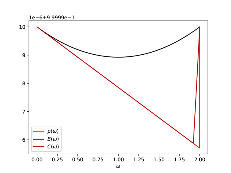
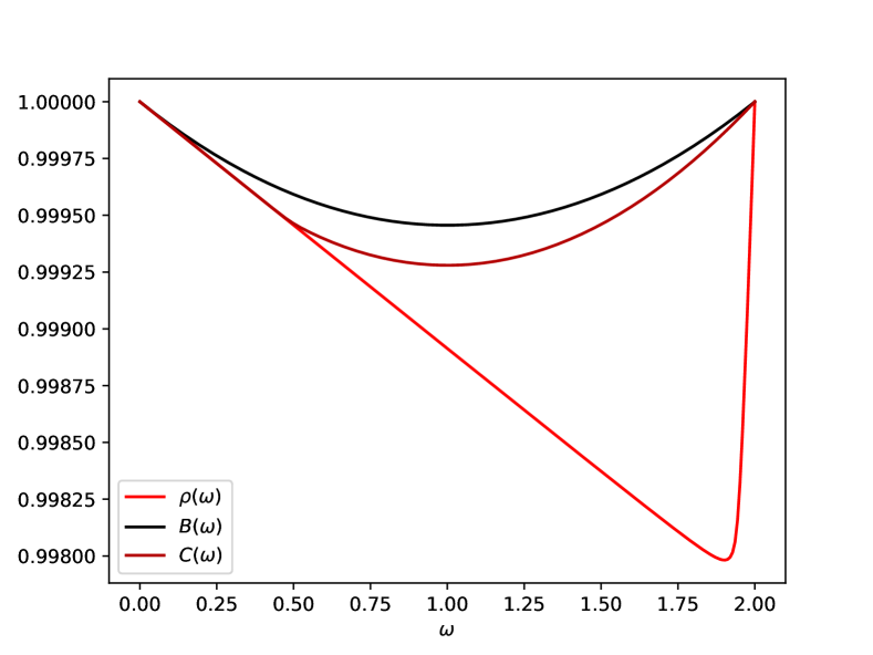
Figure 5: The C-bound’s effectiveness, and the resulting over-relaxation, is more significant for ill-conditioned problems. Random matrices: $50\times 50$ on the left with condition number $\kappa({\boldsymbol{A}})=61705.3$ and $75\times 50$ on the right with condition number $\kappa({\boldsymbol{A}})=110.2$.

For ease of exposition we have presented the analysis for when a single row is chosen at each step of the iteration in (1). For block methods, a subset of rows are chosen at each step (e.g., subsets uniformly chosen), and each $\boldsymbol{P}_{i}$ is a projector into the span of the chosen subset. The analysis can be directly extended as the expected projector $\operatorname{\mathbb{E}}\left[\boldsymbol{P}\right]=\frac{1}{M}\sum_{i}\boldsymbol{P}_{i}$ and $\operatorname{\mathbb{E}}\left[\boldsymbol{P}\otimes\boldsymbol{P}\right]=\frac{1}{M}\sum_{i}\boldsymbol{P}_{i}\otimes\boldsymbol{P}_{i}$ (here $M$ denotes the total number of choices for each step) are similarly defined for block schemes where Lemma 1 applies. Furthermore, the ingredients in (8) can be calculated online during iterations.

The presented approach for bounding the spectral radius is a specialization of Weyl’s inequality and hence is applicable to other applications of eigenvalue perturbation theory. As mentioned earlier, the effectiveness of over-relaxation produced by the C-bound depends on the gap between the two eigenvalues $\mu_{2}$ and $\mu_{1}$ and the gap between $\mu_{1}$ and $\xi$. In particular, for well-conditioned problems the optimal over-relaxation values $\omega$ provided by the C-bound are close to $1$ and ill-conditioned problems push the over-relaxation value towards $2$.

Figure 5 shows the spectral radius of $\boldsymbol{\mathcal{A}}$ for a pair of random matrices subjected to the Kaczmarz algorithm. The left plot shows the performance of the C-bound, and the resulting over-relaxation, on a $50\times 50$ matrix with a relatively large condition number and the right plot shows an overdetermined system $75\times 50$ that has a relatively small condition number and a small gap between the two smallest singular values. Figure 6, first row, shows the performance of the C-bound on the Hilbert matrix for the Gauss-Seidel algorithm since it is symmetric positive definite. As the condition number grows rapidly the figure shows the performance for $n=2,3,4$; the trend continues with larger $n$. The second row shows the performance on a non-symmetric cousin of the Hilbert matrix, called the Parter matrix (Moler, 2025) with the Kaczmarz algorithm for $n=5,20$ and $50$.

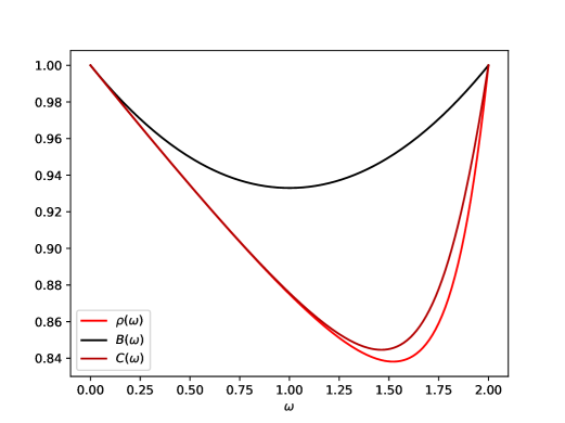
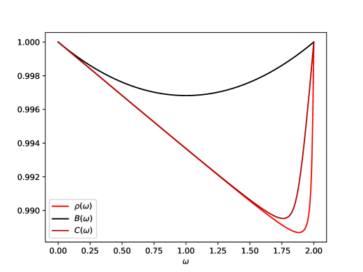
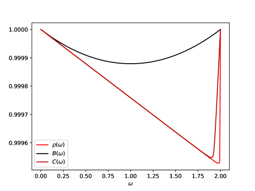
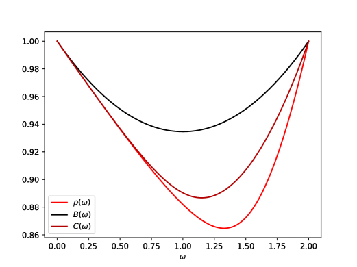
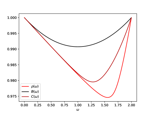
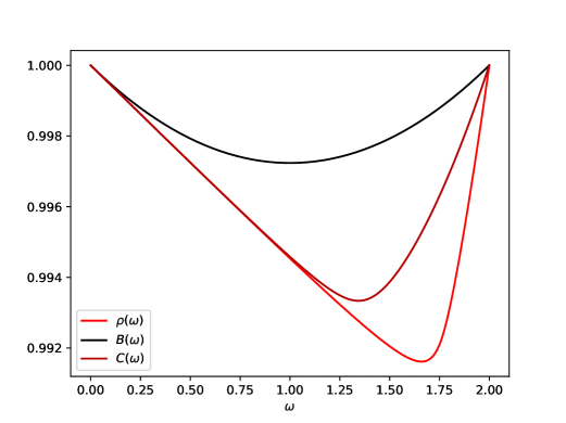
Figure 6: The top row shows the performance of the C-bound for the Hilbert matrix for $n=2$ (left), $n=3$ (middle) and $n=4$ (right) with the Gauss-Seidel algorithm. The trend continues for larger $n$. The bottom row shows the performance on the non-symmetric Parter matrix for $n=5$ (left), $n=20$ (middle) and $n=50$ (right) with the Kaczmarz algorithm.

The specific C-bound presented in (9) can be generalized in several directions. When $\mu_{1}=\mu_{2}$ the C-bound coincides with the B-bound providing no over-relaxation. In this case or when $\mu_{2}$ and $\mu_{1}$ are close or when several eigenvalues are close to $\mu_{1}$, one can build a bound by clustering those eigenvalues and using the next eigenvalue of $\operatorname{\mathbb{E}}\left[\boldsymbol{P}\right]$ that has a substantial gap for building the C-bound. As Lemma 16 suggests, $\xi$ is the result of restriction of $\boldsymbol{\mathcal{C}}$ to the smallest eigenspace, $\boldsymbol{V}_{1}(\boldsymbol{\mathcal{B}})$, and in this generalized setting $\xi$ will be defined to be the spectral radius of $\boldsymbol{\mathcal{C}}$ restricted to the eigenspace corresponding to the eigenvalues that are clustered with $\mu_{1}$. Another direction is to build C-bounds by designing surrogate $\boldsymbol{\mathcal{C}}^{\star}$ in subspaces larger than two. A challenge, from a practical viewpoint, is to derive bounds based on minimal ingredients.

A consequence of Lemma 7 is that irreducibility is a convenient but not necessary assumption for the validity of the C-bound. Irreducibility guarantees that the spectral radius of $\boldsymbol{\mathcal{A}}$ is unique for any relaxation value $\omega$ and therefore at $\omega=0$ it implies that $\mu_{1}$ is simple and ${\bf v}_{1}(\operatorname{\mathbb{E}}\left[\boldsymbol{P}\right])$ is one dimensional in (8). In the absence of irreducibility one needs $\mu_{1}$ to be a simple eigenvalue so that ${\bf u}_{1}$ is unique (up to sign). When $\mu_{1}$ is a repeated eigenvalue, $\xi$ needs to be defined based on a ${\bf u}_{1}$ in the eigenspace ${\bf v}_{1}(\operatorname{\mathbb{E}}\left[\boldsymbol{P}\right])$ that attains the maximum value in (8). Finally, irreducible problems are dense in the sense that any reducible problem ${\boldsymbol{A}}{{\bf x}}={{\bf b}}$ can be infinitesimally perturbed to an irreducible problem. Lemma 7 shows that this fact translates to irreducibility of superoperator $\boldsymbol{\mathcal{A}}$. Since the spectral radius (and the rate of convergence) is a continuous function of the parameters of the system (e.g., ${\boldsymbol{A}}$, $\omega$), the bounds remain valid regardless of irreducibility.

References

- Agaskar et al. (2014) Ameya Agaskar, Chuang Wang, and Yue M Lu. Randomized Kaczmarz algorithms: Exact MSE analysis and optimal sampling probabilities. In 2014 IEEE Global Conference on Signal and Information Processing (GlobalSIP), pages 389–393. IEEE, 2014.
- Aguech et al. (2000) Rafik Aguech, Eric Moulines, and Pierre Priouret. On a perturbation approach for the analysis of stochastic tracking algorithms. SIAM Journal on Control and Optimization, 39(3):872–899, 2000.
- Bach and Moulines (2013) Francis Bach and Eric Moulines. Non-strongly-convex smooth stochastic approximation with convergence rate . Advances in neural information processing systems, 26, 2013.
- Bertsekas (2011) Dimitri P Bertsekas. Incremental proximal methods for large scale convex optimization. Mathematical programming, 129(2):163–195, 2011.
- Bhatia (2009) Rajendra Bhatia. Positive definite matrices. Princeton university press, 2009.
- Censor et al. (2009) Yair Censor, Gabor T Herman, and Ming Jiang. A note on the behavior of the randomized Kaczmarz algorithm of Strohmer and Vershynin. Journal of Fourier Analysis and Applications, 15:431–436, 2009.
- Défossez and Bach (2015) Alexandre Défossez and Francis Bach. Averaged least-mean-squares: Bias-variance trade-offs and optimal sampling distributions. In Artificial Intelligence and Statistics, pages 205–213. PMLR, 2015.
- Deutsch (1995) Frank Deutsch. The angle between subspaces of a Hilbert space. In Approximation theory, wavelets and applications, pages 107–130. Springer, 1995.
- Deutsch and Hundal (1997) Frank Deutsch and Hein Hundal. The rate of convergence for the method of alternating projections, II. Journal of Mathematical Analysis and Applications, 205(2):381–405, 1997.
- Evans and Høegh-Krohn (1978) David E Evans and Raphael Høegh-Krohn. Spectral Properties of Positive Maps on -Algebras. Journal of the London Mathematical Society, 2(2):345–355, 1978.
- Farenick (1996) Douglas Farenick. Irreducible positive linear maps on operator algebras. Proceedings of the American Mathematical Society, 124(11):3381–3390, 1996.
- Galántai (2005) Aurél Galántai. On the rate of convergence of the alternating projection method in finite dimensional spaces. Journal of mathematical analysis and applications, 310(1):30–44, 2005.
- Gordon (2018) Dan Gordon. A derandomization approach to recovering bandlimited signals across a wide range of random sampling rates. Numerical Algorithms, 77(4):1141–1157, 2018.
- Gower and Richtárik (2015) Robert M Gower and Peter Richtárik. Randomized iterative methods for linear systems. SIAM Journal on Matrix Analysis and Applications, 36(4):1660–1690, 2015.
- Hackbusch (2016) Wolfgang Hackbusch. Iterative solution of large sparse systems of equations, volume 95. Springer Cham, 2016. doi: https://doi.org/10.1007/978-3-319-28483-5.
- Hairer (2006) Martin Hairer. Ergodic properties of Markov processes. Lecture notes, 2006.
- Halperin (1962) Israel Halperin. The product of projection operators. Acta Sci. Math.(Szeged), 23(1):96–99, 1962.
- Herman et al. (1978) Gabor T Herman, Arnold Lent, and Peter H Lutz. Relaxation methods for image reconstruction. Communications of the ACM, 21(2):152–158, 1978.
- Jain et al. (2018) Prateek Jain, Sham M Kakade, Rahul Kidambi, Praneeth Netrapalli, and Aaron Sidford. Parallelizing stochastic gradient descent for least squares regression: mini-batching, averaging, and model misspecification. Journal of machine learning research, 18(223):1–42, 2018.
- Kayalar and Weinert (1988) Selahattin Kayalar and Howard L Weinert. Error bounds for the method of alternating projections. Mathematics of Control, Signals and Systems, 1(1):43–59, 1988.
- Leventhal and Lewis (2010) Dennis Leventhal and Adrian S Lewis. Randomized methods for linear constraints: convergence rates and conditioning. Mathematics of Operations Research, 35(3):641–654, 2010.
- Liu and Wright (2016) Ji Liu and Stephen Wright. An accelerated randomized Kaczmarz algorithm. Mathematics of Computation, 85(297):153–178, 2016.
- Moler (2025) Cleve Moler. Matrices at an Exposition, 2025. URL https://blogs.mathworks.com/cleve/2025/03/07/matrices-at-an-exposition/.
- Murata (1999) Noboru Murata. A Statistical Study of On-line Learning, page 63–92. Publications of the Newton Institute. Cambridge University Press, 1999.
- Nedić and Bertsekas (2001) Angelia Nedić and Dimitri Bertsekas. Convergence rate of incremental subgradient algorithms. Stochastic optimization: algorithms and applications, pages 223–264, 2001.
- Nemirovski et al. (2009) Arkadi Nemirovski, Anatoli Juditsky, Guanghui Lan, and Alexander Shapiro. Robust stochastic approximation approach to stochastic programming. SIAM Journal on optimization, 19(4):1574–1609, 2009.
- Nesterov (2012) Yurii Nesterov. Efficiency of coordinate descent methods on huge-scale optimization problems. SIAM Journal on Optimization, 22(2):341–362, 2012.
- Nesterov and Stich (2017) Yurii Nesterov and Sebastian U Stich. Efficiency of the accelerated coordinate descent method on structured optimization problems. SIAM Journal on Optimization, 27(1):110–123, 2017.
- Nutini et al. (2009) Julie Nutini, Mark Schmidt, Behrooz Sepehry, Hoyt Koepke, Issam Laradji, and Alim Virani. Convergence Rates for Greedy Kaczmarz Algorithms, and Faster Randomized Kaczmarz Rules Using the Orthogonality Graph. J. Fourier Anal. Appl, 15(2):262–278, 2009.
- Polyak and Juditsky (1992) Boris T Polyak and Anatoli B Juditsky. Acceleration of stochastic approximation by averaging. SIAM journal on control and optimization, 30(4):838–855, 1992.
- Recht and Ré (2012) Benjamin Recht and Christopher Ré. Toward a noncommutative arithmetic-geometric mean inequality: Conjectures, case-studies, and consequences. In Conference on Learning Theory, pages 11–1. JMLR Workshop and Conference Proceedings, 2012.
- Saad (2003) Yousef Saad. Iterative methods for sparse linear systems. SIAM, 2003.
- Smith et al. (1977) Kennan T. Smith, Donald C. Solmon, and Sheldon L. Wagner. Practical and mathematical aspects of the problem of reconstructing objects from radiographs. Bulletin of the American Mathematical Society, 83(6):1227 – 1270, 1977.
- Solo (1989) Victor Solo. The limiting behavior of LMS. IEEE Transactions on Acoustics, Speech, and Signal Processing, 37(12):1909–1922, 1989.
- Strohmer and Vershynin (2009) Thomas Strohmer and Roman Vershynin. A randomized Kaczmarz algorithm with exponential convergence. Journal of Fourier Analysis and Applications, 15(2):262–278, 2009.
- Tao and Vu (2011) Terence Tao and Van Vu. Random matrices: Universality of local eigenvalue statistics. Acta Mathematica, 206(1):127 – 204, 2011. doi: 10.1007/s11511-011-0061-3. URL https://doi.org/10.1007/s11511-011-0061-3.
- Tu et al. (2017) Stephen Tu, Shivaram Venkataraman, Ashia C Wilson, Alex Gittens, Michael I Jordan, and Benjamin Recht. Breaking locality accelerates block Gauss-Seidel. In International Conference on Machine Learning, pages 3482–3491. PMLR, 2017.
- Widrow and Hoff (1988) Bernard Widrow and Marcian E Hoff. Adaptive switching circuits. In Neurocomputing: foundations of research, pages 123–134. 1988.
- Wilson et al. (2021) Ashia C Wilson, Ben Recht, and Michael I Jordan. A Lyapunov analysis of accelerated methods in optimization. Journal of Machine Learning Research, 22(113):1–34, 2021.
- Wolf (2012) Michael M Wolf. Quantum channels and operations-guided tour. 2012. URL https://mediatum.ub.tum.de/doc/1701036/document.pdf.
- Young (1954) David Young. Iterative methods for solving partial difference equations of elliptic type. Transactions of the American Mathematical Society, 76(1):92–111, 1954.