Entanglement and purity can help to detect systematic experimental errors

Abstract

Measurements are central in all quantitative sciences and a fundamental challenge is to make observations without systematic measurement errors. This holds in particular for quantum information processing, where other error sources like noise and decoherence are unavoidable. Consequently, methods for detecting systematic errors have been developed, but the required quantum state properties are yet unexplored. We develop theoretically a direct and efficient method to detect systematic errors in quantum experiments and demonstrate it experimentally using quantum state tomography of photon pairs emitted from a semiconductor quantum dot. Our results show that entanglement as well as quantum states with a high purity can help to identify systematic errors.

Introduction.—

The results of the past 30 years in quantum information science [1, 2, 3] promise an exciting future for applications such as quantum communication [4, 5, 6], the efficient solving of challenging problems that are hard to tackle for classical computers [7, 8], or the simulation of complex many-body systems with quantum computers [9, 10, 11, 12]. All these applications strongly rely on the correct readout of quantum information via measurements of a quantum system. For instance, quantum state tomography [13] and shadow tomography [14, 15] are typical examples of an information readout procedure, where a finite number of measurements on equally prepared state copies is carried out. In state tomography, however, measurement errors can lead to nonphysical estimates of the quantum state. In practice, statistical and systematic errors are the most prominent types of measurement errors, and they are relevant not only in quantum state tomography, but also in other tools for analysing quantum systems [16, 17, 18, 19, 20, 21].

Statistical errors in measurements arise from finite statistics: Every experiment is repeated only a finite number of times, and the observed frequencies of outcomes do not necessarily correspond to the outcome probabilities. In quantum state tomography this can lead to nonphysical state estimates. Current literature addresses statistical errors by discussing confidence regions of estimators [22, 23, 24, 25, 26, 27] or by using statistical tools [28] to find the necessary number of measurement repetitions to recover a physical state estimate [29].

In contrast to statistical errors, systematic errors originate from various environmental influences as well as imperfections and various works discussed the impact of errors like misalignment of the measurement basis. This concerns determining the state fidelity and entanglement witnesses [30], systematic errors due to bias in quantum state estimators [31, 32], robustness of tomography schemes [33, 34, 35] and the characterization of photon-detectors [36, 37]. All these results emphasize the variety and relevance of statistical and systematic errors in the field of quantum information.

This naturally leads to the question of how to distinguish statistical from systematic errors. Both types of errors can have similar effects, but statistical errors can be suppressed by more repetitions of an experiment, while systematic errors may point at fundamental flaws in the design of an experiment. In Ref. [38] methods to construct from the measurement data witnesses to certify systematic errors have been proposed. Moreover, Ref. [39] discussed the chi-squared goodness-of-fit test to assess the quality of the reconstructed state with respect to a previously chosen model and how to modify the test appropriately for states close to the border of the physical state space.

In this work we first develop theoretically a direct and efficient method to detect systematic errors. Then, we experimentally implement the scheme using entangled photon pairs emitted by a semiconductor quantum dot [40]. We employ strain tuning on the source [41, 42] to generate two-photon polarization states with a varying degree of entanglement and purity. We use quantum state tomography as an example for an involved quantum information task, but one can adjust the ideas for other quantum tasks and experimental platforms as well. Our findings demonstrate that even quantum states with a low purity can be sensitive enough to signal the presence of systematic errors. Moreover, if two or more particles are considered, entanglement of the probe states can be essential in our scheme to detect the error.

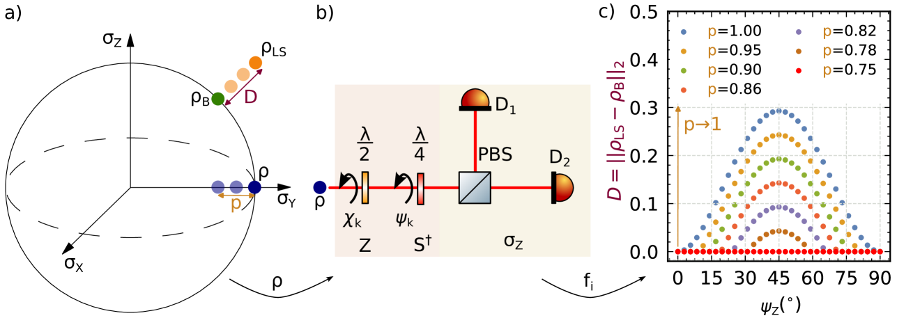
Figure 1: Illustration of the detection scheme for systematic errors in a simple setting. a) The Bloch sphere is the physical state space of a single qubit. The blue dot denotes a quantum state $\rho$, which should be determined from Pauli measurements. A severe systematic or statistical error can lead to a least-squares estimate ${\rho_{\text{LS}}}$ (orange dot) outside of the state space, and thus the distance $D$ (purple arrow) between a physical (but biased) estimate ${\rho_{\text{B}}}$ of Eq. (2) (green dot) is finite. If this distance $D$ persists for large statistical samples, this is a signature of a systematic error. Note that the distance $D$ decreases when the underlying state $\rho$ has lower purity $p={\operatorname{Tr}}(\rho^{2})$, as suggested by the purple and yellow arrows. b) Single-qubit Pauli measurements for polarized photons: In the pink area the $k$-th Pauli measurement setting for obtaining the two frequencies $f_{i}$ and $f_{j}$, corresponding to the eigenvalues, is adjusted by the rotations $\chi_{k}$ and $\psi_{k}$ of the half-wave plate ($Z$ gate) and the quarter-wave plate ($S^{\dagger}$ gate), respectively. The polarizing beam splitter (PBS) together with single-photon detectors (D1) and (D2) implement the ${\sigma_{\text{Z}}}$ basis measurement, and they are depicted in the yellow area. c) The calculated distance $D$ depends on the adjustment angle $\psi_{Z}$ of the Pauli $Z$ basis, and its magnitude decreases with the purity of the true, underlying state $\rho=\ket{\mathrm{i}}\bra{\mathrm{i}}$, with the state $\ket{\mathrm{i}}$ chosen to be the eigenstate of ${\sigma_{\text{Y}}}$. The maximum $D$ at $\psi_{\text{Z}}=$45\text{\,}\mathrm{\SIUnitSymbolDegree}$$ occurs when ${\sigma_{\text{Y}}}$ is measured instead of ${\sigma_{\text{Z}}}$, and for a purity $p=0.75$ the error cannot be detected anymore.

Measurement schemes for tomography.—

In order to determine the quantum state, one measures a set of tomographically complete measurement operators $\operatorname{P}_{i}$ on $N$ copies of the quantum state, described by the density operator $\rho$. The operators $\operatorname{P}_{i}$ are Hermitian and constitute a basis to the space of all observables where $i$ denotes a specific measurement outcome. Local Pauli measurements [43] are a frequently used tomographically complete set of measurements for qubits, which consists of all $3^{n}$ strings of Pauli measurements acting on $n$ qubits. From now on, we focus on these, albeit our idea works for other measurement schemes [44, 45, 46, 47, 48] as well. Quantum state tomography determines $\rho$ from the experimentally observed frequencies $f_{i}$, which are an approximation of the outcome probabilities, and are defined as the number of times the outcome of a tomographically complete set of observables $\operatorname{P}_{i}$ occurs relative to $N$. In the limit of $N\to\infty$ one recovers the ”true” underlying outcome probabilities as predicted by Born’s rule.

Biased and unbiased state estimators.—

Once the outcome frequencies are obtained from the measurement procedure, an estimate for the quantum state can be determined. For that, different kinds of estimators exist, which may be unbiased or biased. By definition, unbiased estimators have the property that the expectation value of the estimator equals the true value. From the fact that the set of allowed density matrices is constrained by the positivity of their eigenvalues, one can show that unbiased estimators deliver necessarily nonphysical states [31], meaning that the predicted state ${\rho_{\text{U}}}$ may be not positive semidefinite.

The least-squares estimator is an unbiased estimator on which we focus from now on. It is defined for single qubits as follows:

$${\rho_{\text{LS}}}=\frac{1}{2}\Big{(}\openone+\sum^{3\cdot 2}_{i=1}f_{i}P_{i}\Big{)},$$ (1)

where $f_{i}$ are the experimentally observed frequencies. For $n$-qubit states the sum in Eq. (1) iterates over all $4^{n}-1$ non-trivial tensor products of Pauli measurements, each having two possible outcome frequencies. Clearly, it can occur that frequencies $f_{i}$ are observed where the resulting estimate ${\rho_{\text{LS}}}$ has negative eigenvalues. This is more likely, if the underlying quantum state $\rho$ has a high purity and lies close to the surface of the Bloch sphere, see also Fig. 1a.

On the other hand, in order to ensure valid quantum states, one may impose additional positivity constraints. This necessarily leads to biased state estimators. For example one may take as an estimate ${\rho_{\text{B}}}$ the closest positive semidefinite state to the least-squares estimate ${\rho_{\text{LS}}}$ with respect to the squared Hilbert-Schmidt norm [26], which can be expressed as the following optimization problem,

$${\rho_{\text{B}}}=\operatorname*{arg\,min}_{\begin{subarray}{c}\operatorname{Tr}(\varphi)=1\\ \varphi\succcurlyeq 0\end{subarray}}||{\rho_{\text{LS}}}-\varphi||^{2}_{2}.$$ (2)

Clearly, if only statistical fluctuations are present, the unbiased estimator ${\rho_{\text{LS}}}$ converges to a physical state in the limit of many repetitions of the experiment, $N\rightarrow\infty.$ If, however, a severe systematic error occurs this is not necessarily the case. One may end up with very different estimates ${\rho_{\text{LS}}}$ and ${\rho_{\text{B}}}$, which results in a non-negligible distance $D$ between the estimates,

$$D=||{\rho_{\text{LS}}}-{\rho_{\text{B}}}||_{2}=\operatorname{Tr}\Big{[}({\rho_{\text{LS}}}-{\rho_{\text{B}}})^{2}\Big{]}^{1/2},$$ (3)

which utilizes the Hilbert-Schmidt norm as a metric. So, if $D>0$ even for large $N$, this is a signature of systematic errors. This is the core idea of our method to recognize systematic errors.

In Fig. 1 we illustrate the concept of our systematic error detection method on a single-qubit system. In Fig. 1a we see the Bloch sphere, the physical state space of a single qubit, and as blue dots the state $\rho$. We assume that a (for demonstration purposes) severe systematic or statistical error occurs, which leads to a least-squares estimate ${\rho_{\text{LS}}}$ (orange dot) far outside of the Bloch sphere. Consequently, the distance $D$, purple arrow, between the biased estimate ${\rho_{\text{B}}}$, green dot, is non-negligible. If we apply a depolarization channel to $\rho$, the purity $p$ of $\rho$ reduces, indicated by the yellow arrow between the blue dot and the transparent blue dots. With the decrease of the state purity $p$ the distance $D$ decreases as well (see transparent orange dots).

Fig. 1b shows the single-qubit Pauli measurement setting for qubits implemented by the polarization of photons. The $k$-th basis measurement setting allows to determine the two frequencies $f_{i}$ and $f_{j}$ that correspond to its eigenvalues, and is adjusted in the pink area by the rotations $\chi_{k}$ and $\psi_{k}$ of the phase gates $Z$ and $S^{\dagger}$. The phase gates $Z$ and $S^{\dagger}$ correspond to a half- ($\lambda/2$) and quarter-wave ($\lambda/4$) plate, respectively. Subsequently, the basis measurement ${\sigma_{\text{Z}}}$ is performed in the yellow area, which is implemented by a polarizing-beam splitter (PBS) followed by two photon detectors (D1, D2). Fig. 1c shows the calculated results for the distance $D$ of Eq. (3) as function of the basis adjustment angle $\psi_{\text{Z}}$ for the true, underlying state, which we have chosen to be $\rho=\ket{\mathrm{i}}\bra{\mathrm{i}}$, i.e. the $+1$ eigenstate of the Pauli $\mathrm{Y}$ matrix, on which we have applied a depolarizing channel to obtain purity values from $0.75$ to $1$. Note that we simulate that all Pauli measurements are correctly observed except for the ${\sigma_{\text{Z}}}$ basis, for which we vary the alignment angle $\psi_{\text{Z}}$, where $0\text{\,}\mathrm{\SIUnitSymbolDegree}$ corresponds to a perfectly adjusted ${\sigma_{\text{Z}}}$ basis. The maximum of the distance $D$ is obtained for $\psi_{\text{Z}}=$45\text{\,}\mathrm{\SIUnitSymbolDegree}$$, where the ${\sigma_{\text{Y}}}$ basis is measured instead. Furthermore, we see that the distance $D$ decreases with the state purity, and it vanishes for a purity value of $p_{\text{min}}=0.75$. We provide more details on this example in Appendix B.1.1.

Rigorous formulation of the method.—

The mere definition of $D$ is not sufficient to certify systematic errors because it does not allow to distinguish between statistical and systematic errors. Concentration bounds have proven to be useful statistical tools to find the probability that a quantity obtained by finite experimental repetitions deviates from its true mean. We follow the spirit of Ref. [27], and interpret quantum state tomography as sum of independent, zero-mean, random vectors such that we can utilize the vector Bernstein inequality to derive the following proposition, see Appendix C for details.

Proposition 1.

Let ${\rho_{\text{LS}}}$ and ${\rho_{\text{B}}}$ be the least-square and biased estimate ${\rho_{\text{B}}}$ from Eq. (1) and Eq. (2), respectively. The least-squares estimate ${\rho_{\text{LS}}}$ is determined from the observed frequencies $f_{i}$, which are obtained from measuring $N$ identical state copies of the true underlying quantum state $\rho$. Then, the probability $\delta_{\text{sta}}$ that the distance $D$ of Eq. (3) between ${\rho_{\text{LS}}}$ and ${\rho_{\text{B}}}$ is greater equal than $\tau$ obeys:

$$\delta_{\text{sta}}=\mathbb{P}\left[D\geqslant\tau\right]\leq 8\exp\left[-\frac{{N}\,\tau^{2}}{2\times 5^{n}}\frac{3}{3+\sqrt{2}\tau/\sqrt{5^{n}}}\right],$$ (4)

where $n$ is the number of qubits on which local Pauli measurements are measured.

This bounds the probability $\delta_{\text{sta}}$ that only statistical errors are causing a distance $D>\tau$ between ${\rho_{\text{LS}}}$ and ${\rho_{\text{B}}}$, and if this is smaller than a threshold fixed beforehand, one can reject the hypothesis that only statistical errors occur. Consequently, if the distance $D$ of Eq. (3) is significantly larger than the corresponding $\tau$, the systematic error test successfully detects a systematic error with confidence level $1-\delta_{\text{sta}}$.

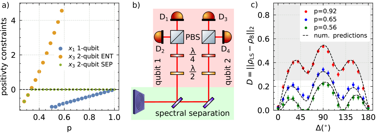
Figure 2: a) Capability of single-qubit states (blue) as well as entangled (orange) and separable (green) two-qubit states to detect the error of exchanging ${\sigma_{\text{Y}}}$ and ${\sigma_{\text{Z}}}$ on qubit one. We show the results of the maximization problem of Eq. (6) as a function of the purity $p$ of the true underlying state $\rho$, and we see that only entangled states return values $x_{3}$ beyond the dashed line, which means they can detect this error. b) Experimental setup used for single-qubit Pauli measurements of an entangled, two-qubit quantum state from a quantum dot [49, 41]. State preparation and separation of the two qubits takes part in the green area, and in the red area the individual single-qubit Pauli measurements are performed. c) We add the same offset $\Delta$ on qubit one for each measurement setting $k$, i.e. $\psi_{k}=\psi_{k}^{\mathrm{theo}}+\Delta$. The experimental results for the distance $D$ between least-squares $({\rho_{\text{LS}}})$ and the biased estimate $({\rho_{\text{B}}})$ are shown depending on $\Delta$ as red, blue and green dots for a purity ranging from $0.56$ to $0.92$. The measured data points are in accordance with the lines from the simulated predictions for all three quantum states. The confidence level to detect a systematic error begins with $90\%$ for a distance $D\geq 0.25$ (grey area), which allows detection of almost all errors for highly entangled states (red points).

Necessary State Properties for Error Detection.—

The single-qubit example from above highlights that the purity of the state is relevant to detect the errors. So, we investigate the minimal purity, for which there exists a one- or two-qubit state $\rho$, which allows to detect a local single-qubit error on qubit one. We assume that the systematic error on qubit one is such that the corrupted Pauli measurements $\tilde{\sigma}_{\mu}$ are linear combinations of all three, true Pauli measurements:

$$\tilde{\sigma}_{\mu}=\sum^{3}_{\nu=1}\operatorname{M}_{\mu\nu}\sigma_{\nu},$$ (5)

where the rows of the misalignment matrix $\operatorname{M}$ have to be normalized to ensure that the expectation values of the Pauli observables are restricted to $\pm 1$. The error $\operatorname{M}$ influences all observed frequencies on qubit one and, as a consequence from Eq. (1), we obtain a corrupted least-squares estimate $\tilde{\rho}_{\text{LS}}$.

To check whether this estimate corresponds to a valid state, we use results on the positivity constraints of multi-qubit states [50, 51]. Any quantum state $\rho$ has to have positive eigenvalues, and consequently, it obeys a set of inequalities which can be formulated as $\zeta_{l}(\rho)\leq 0$ [50, 51]. The number of inequalities $l$ is the total number of eigenvalues minus one, and scales with the number of qubits $n$ as $l=2^{n}-1$. If any of the parameters $\zeta_{l}(\tilde{\rho}_{\text{LS}})$ is greater than zero, then $\tilde{\rho}_{\text{LS}}$ has a negative eigenvalue, and one can use our method to detect the error. To find the minimal necessary purity of $\rho$, we start with the minimal purity $\wp={\operatorname{Tr}}(\rho^{2})=1/4$ of a maximally mixed two-qubit state $\rho=\openone/4.$ Then, we increase the variable purity $\wp$ of the underlying state and ask whether for the estimate $\tilde{\rho}_{\text{LS}}$ one of the positivity constraints is violated,

$$x_{l}=\max_{\rho\;\rm{:}\;{\operatorname{Tr}}(\rho^{2})\leq\wp\;\rm{and}\;\zeta_{k}(\rho)\leq 0}\zeta_{l}(\tilde{\rho}_{\text{LS}}).$$ (6)

This depends on the misalignment matrix $\operatorname{M}$, of course, but interestingly one can directly solve this, see Appendix B.1 for details. To distinguish entangled from separable probe states, one may add a constraint for the partial transposition of $\rho$ to be positive semidefinite. This restricts the optimization to separable states only, and allows to study whether quantum entanglement can help in analysing systematic errors.

Concretely, we determined analytically the minimal necessary state purity $p_{\text{min}}$ in dependence on the adjustment error in the ${\sigma_{\text{Y}}}$ and ${\sigma_{\text{Z}}}$ basis, which we model by the misalignment matrix on the first qubit,

$$\operatorname{M}_{1}=\left(\begin{array}[]{lll}1&0&0\\ \sin{(\beta)}\sin{(\alpha)}&\cos{(\alpha)}&\cos{(\beta)}\sin{(\alpha)}\\ \sin{(\delta)}\sin{(\gamma)}&\cos{(\delta)}\sin{(\gamma)}&\cos{(\gamma)}\end{array}\right).$$ (10)

Note that this is indeed already the most general error on a single qubit in the formalism of misalignment matrices, since rotations of the ${\sigma_{\text{X}}}$ measurement can be counteracted by a local unitary transformation. We check systematically for all combinations $\alpha,\beta,\gamma,\delta$ of $\{0,\frac{\pi}{8},\frac{\pi}{4},\frac{3\pi}{8},\frac{\pi}{2}\}$. For each setting of angles we determined $p_{\text{min}}$ of single-qubit states as well as for separable two-qubit states and general (potentially entangled) two-qubit states.

First, we find without any exception that for two-qubit quantum states less purity is sufficient for the detection of systematic errors compared to single-qubit systems. The values of $p_{\text{min}}$ for two-qubit systems are between $0.29$ and $0.34$ which is significantly below the smallest possible purity of the maximally mixed single-qubit state $0.5$. Still, this result has to be handled with care, as purities of states with a different number of qubits are difficult to compare.

Furthermore, we find that the error of exchanging ${\sigma_{\text{Y}}}$ and ${\sigma_{\text{Z}}}$ (that is, $\alpha=\gamma=\pi/2$ and $\beta=\delta=0$), which corresponds to a partial transposition on the first qubit, gives different results for entangled entangled and product states. In particular, only entangled states are suitable to detect this error, see also Appendix B.3 for a detailed discussion. In Fig. 2a we show the results for the positivity constraints of Eq. (6) depending on the state purity $p$ where the error is the described exchange on the first qubit. The orange and green dots are the $x_{3}$ values for entangled and separable states, respectively, and the values $x_{1}$ for single qubits are represented by the blue dots. Only the values of the entangled state exceed the black dashed line at $x_{l}=0$ at $p_{\text{min}}=0.33$, which means that there exist a state that is suitable to detect the error. We stress that an unintentional exchange of the wave plates in Fig. 1b is an example for a partial transposition error and thus it can only be detected by entangled states.

Experimental Demonstration.—

We demonstrate that our method is practically feasible by using entangled two-qubit photonic states emitted by a GaAs quantum dot [52]. More specifically, we use a recently developed device [41] in which the quantum dot is embedded in a circular Bragg resonator and integrated on a micromachined piezoelectric substrate, offering two specific advantages. The optical microcavity enhances photon collection. The achieved coincidence rate allows to perform quantum tomography as a function of a measurement variable and collect enough data to properly estimate the statistical uncertainty while ensuring stability of the experimental conditions during acquisition. The piezoelectric substrate allows strain tuning of the excitonic fine structure of the emitter, which is an effective approach to modify the purity of the photon pair at the source level [52, 41, 42]. Fig. 2b shows a simplified sketch of the experimental setup, which includes the light emission from the quantum dot followed by spectral filters to split the state into two single-qubit measurement paths. We consider the case in which all measurement settings $k$ on qubit one are exposed to constant angular offset $\Delta$ in the quarter-wave plate adjustment angle $\psi_{k}=\psi_{k}^{\mathrm{theo}}+\Delta$. This systematic error is relevant in laboratory practice because it corresponds to an error in the alignment of the wave plates.

Fig. 2c shows the experimental results for the distance $D$ as function of the offset $\Delta$ for quantum states with three different purity values from $0.56$ to $0.92$, which have been obtained from a single quantum dot [42, 52, 41] under different conditions of induced strain. The distance $D$ increases as function of the purity, which is in agreement with our previous discussion. The black line is the simulation of the expected distance $D$ as function of $\Delta$ by using the correctly measured quantum states at $\Delta=0$. We see that the simulation agrees with the measurement result. We underline that our method detects systematic errors with a confidence level of $90\%$ and above for distances $D\geq 0.25$. These distances can be reached for nearly all errors $\Delta$ for highly entangled states. We refer to Appendix D for details on the statistical evaluation and the confidence level of the experimental results.

The present experimental results underline that our method is a valuable tool for detecting possible systematic errors in the measurement. Moreover, the results demonstrate that the purity of the quantum state affects the error detection capabilities, as previously shown. We provide a non-exhaustive discussion on the detection of other common systematic errors on qubits implemented by the photon’s polarization in the Appendix F.

Discussion.—

Systematic errors in the readout of quantum information may be severe and hard to recognize. We have introduced a user-friendly method to detect systematic errors, which bases on comparing the estimates from an unbiased and biased estimator on the same measurement data, and we have determined the probability that the deviation between the estimates is caused by a systematic error in dependence of the number of measurement repetitions. Furthermore, we have analytically determined the smallest necessary state purity such that there exists a state that is suitable to detect a given single-qubit error. We have reported that entangled states can be the most useful states for detecting local single-qubit errors. Finally, we have experimentally demonstrated the applicability of our error detection method for Pauli measurements of a two-qubit photonic state.

An experimentally relevant extension of this work is to analyze the role of correlated errors. In this scenario, it is especially interesting to study the performance of entangled states. Future studies regarding the role of multiple single-qubit errors are also highly desirable. In fact, one can show that two errors may cancel each other such that not even an entangled state would be sufficient to detect it, (see Appendix B.3.3 for an example). Closely related to this aspect is the search for a suitable modification of our method that enables to localize the qubit on which the error occurs. We predict that this work and its future developments will help researchers design their experiments and offer a valuable tool for the faithful implementation of quantum information processing and quantum communication protocols.

Acknowledgments.—

JF is grateful to W. Dür for supporting this project and thanks T. Kraft, C. de Gois, T. Fromherz, C. Schimpf, and J. Neuwirth for fruitful discussions. JF’s research is funded in whole or in part by the Austrian Science Fund (FWF) 10.55776/P36010. For open access purposes, the author has applied a CC BY public copyright license to any author accepted manuscript version arising from this submission. OG was supported by the Deutsche Forschungsgemeinschaft (DFG, German Research Foundation, project numbers 447948357 and 440958198), the Sino-German Center for Research Promotion (Project M-0294), and the German Ministry of Education and Research (Project QuKuK, BMBF Grant No. 16KIS1618K). The project is funded within the QuantERA II Programme that has received funding from the EU H2020 research and innovation programme under GA No. 101017733 via the project QD-E-QKD. The authors also acknowledge support from MUR (Ministero dell’Università e della Ricerca) through the PNRR MUR project PE0000023-NQSTI and the European Union’s Horizon Europe research and innovation program under EPIQUE Project GA No. 101135288, Ascent+ project GA No. 871130, the FWF via the Research Group FG5, and the cluster of excellence quantA [10.55776/COE1] as well as the Linz Institute of Technology (LIT) and the LIT Secure and Correct Systems Lab, supported by the State of Upper Austria. THL acknowledges funding from the BMBF through the Project Qecs (FKZ: 13N16272).

Author contributions.—

JF and OG developed the theory. JF implemented the source code and performed the calculations. JF, FBB, TMK, MBR, QB, SFCdS, SS, SH, THL, AR and RT worked at the design and fabrication of the QD sample. The measurements were conducted by FBB, AL, and MB, and RT coordinated the measurements. JF analyzed the results with the help of FBB. JF and OG coordinated the project. RK provided conceptual guidance/assistance throughout the early stages of this project. JF and OG wrote the manuscript with the help of FBB, TMK, and RT. All authors provided fruitful suggestions for improving the manuscript.

Availability of data and source code.—

The measurement data and source code that support the results of this work are provided upon reasonable request to FBB and JF, respectively.

Appendix A Quantum State Estimators

In this section we review briefly the definition of a tomographically complete set of measurements. We continue with a summary on biased and unbiased quantum state estimators. In particular, we focus on the least-squares estimator and the convex optimization problem returning the closest physical estimate to the linear inversion estimate, as we have introduced in the main text. To provide the reader with alternatives for state estimators, we briefly explain the maximum-likelihood estimators.

A.1 Tomographically Complete Set of Measurements

A tomographically complete set of measurements is a set of hermitian operators that constitutes a basis to the operator space $\mathcal{L}(\mathbb{H}_{d})$, and allows to fully reconstruct the pre-measurement state from its expectation values. For instance the set of Pauli observables $\{\sigma_{\operatorname{X}},\sigma_{\operatorname{Y}},\sigma_{\operatorname{Z}}\}$ is an example for a tomographically complete set of measurements on a single qubit. One can write a tomographically complete set of operators as an informationally complete positive operator-valued measure (IC POVM), which is a set of hermitian, positive semidefinite operators $\operatorname{P}_{i}\in\mathbb{H}_{d}$, which return unique probability distributions for two different states $\rho\neq\sigma$. In order to normalize the returned probability distributions we demand that $\sum^{m}_{i=1}\operatorname{P}_{i}=\openone$ holds. The measurement of a quantum state $\rho\in\mathcal{L}(\mathbb{H}_{d})$ results in one of the outcomes $i\in\left\{1,\dots m\right\}$ and the probability $[p]_{i}$ that outcome $i$ is observed is given by Born’s rule:

$$[p]_{i}={\operatorname{Tr}}(\operatorname{P}_{i}\rho),$$ (11)

where $[p]_{i}$ denotes the $i$-th component of the probability vector $p\in\mathbb{R}^{m}$. It is impossible to directly access the probabilities, Eq. (11), from a single copy of $\rho$, but by performing a sequence of measurements on $N$ identically prepared copies of $\rho$ one can estimate outcome frequencies $f_{N}$ for the probabilities given by Born’s rule:

$$[f_{N}]_{i}=\frac{n_{i}}{N},$$ (12)

where $n_{i}$ is the number of times the outcome $i$ is observed and in the limit of $N\rightarrow\infty$ the observed frequencies correspond to the true probabilities.

A.1.1 Single-Qubit Pauli Basis Measurements

A widely used tomographically complete set of measurements are local single-qubit Pauli basis measurements. The set of operators $\operatorname{P}_{i}$ for Pauli basis measurements written as an IC POVM on a single-qubit system is as follows:

$$\operatorname{P}_{i}=\left\{\frac{1}{3}\ket{\sigma^{+}_{\mathrm{X}}}\bra{\sigma^{+}_{\mathrm{X}}},\frac{1}{3}\ket{\sigma^{-}_{\mathrm{X}}}\bra{\sigma^{-}_{\mathrm{X}}},\dots\frac{1}{3}\ket{\sigma^{-}_{\mathrm{Z}}}\bra{\sigma^{-}_{\mathrm{Z}}}\right\},$$ (13)

which corresponds to the projections on the eigenstates of the Pauli matrices. Note that the normalization factor $3$ corresponds to the total number of different Pauli basis measurement settings. If we implement single-qubit Pauli basis measurements on larger systems, the set of tomographically complete measurements contains all tensor products of the states in Eq. (13). For the two-qubit system we investigate the main text, we obtain the following $36$ operators

$$\operatorname{P}_{i}=\Bigg{\{} \frac{1}{9}\ket{\sigma^{+}_{\mathrm{X}}}\bra{\sigma^{+}_{\mathrm{X}}}\otimes\ket{\sigma^{+}_{\mathrm{X}}}\bra{\sigma^{+}_{\mathrm{X}}},\dots,$$

$$\frac{1}{9}\ket{\sigma^{-}_{\mathrm{Z}}}\bra{\sigma^{-}_{\mathrm{Z}}}\otimes\ket{\sigma^{-}_{\mathrm{Z}}}\bra{\sigma^{-}_{\mathrm{Z}}}\Bigg{\}},$$ (14)

where the prefactor of $9$ corresponds again to the number of distinct Pauli basis measurement settings.

A.2 Unbiased Estimators

In general, the least-squares estimator ${\rho_{\text{LS}}}$ is obtained from the inversion of the linear map $\mathcal{A}:\mathcal{L}(\mathbb{H}_{d})\mapsto\mathbb{R}^{m}$, which has been induced by Born’s rule Eq. (11). If the map $\mathcal{A}$ is injective, it can be inverted as follows:

$${\rho_{\text{LS}}}=\left(\mathcal{A}^{\dagger}\mathcal{A}\right)^{-1}\left(\mathcal{A}^{\dagger}\left(f_{N}\right)\right),$$ (15)

where $f_{N}$ are the observed frequencies. The actual expression for Eq. (15) depends on the operators $P_{i}$, and in the following we discuss the case of single-qubit Pauli basis measurements.

A.2.1 Linear Inversion for Single-Qubit Pauli Measurements

In this subsection we use the convention $(1,\operatorname{Tr(\sigma_{\operatorname{X}}\rho)},\operatorname{Tr(\sigma_{\operatorname{Y}}\rho)},\operatorname{Tr(\sigma_{\operatorname{Z}}\rho)})$ to parameterize the Bloch vector as vector in $\mathbb{R}^{4}$. By this convention we mean to express states as linear combination of the identity and the Pauli matrices, whereby for the latter their expectation values serve as coefficients. We represent the linear map $\mathcal{A}$ as matrix $\operatorname{A}$ by taking into account our convention for vectors:

$$\operatorname{A}=\frac{1}{6}\left(\begin{array}[]{cccc}1&1&0&0\\ 1&-1&0&0\\ 1&0&1&0\\ 1&0&-1&0\\ 1&0&0&+1\\ 1&0&0&-1\end{array}\right).$$ (22)

We use the Moore-Penrose pseudo inverse [53, 54] to invert the linear map induced by Born’s rule, and thus, the least-squares estimator for local Pauli measurements of a single-qubit is given as follows

$${\rho_{\text{LS}}} =\left(\operatorname{A}^{T}\operatorname{A}\right)^{-1}\operatorname{A}^{T}f$$

$$=\frac{1}{2}\left(\begin{array}[]{cccccc}1/3&1/3&1/3&1/3&1/3&1/3\\ 1&-1&0&0&0&0\\ 0&0&1&-1&0&0\\ 0&0&0&0&1&-1\end{array}\right)\left(\begin{array}[]{c}f_{0}\\ f_{1}\\ f_{2}\\ f_{3}\\ f_{4}\\ f_{5}\end{array}\right)$$ (33)

$$=\frac{1}{2}\left(\begin{array}[]{cccc}1,&f_{1}-f_{2},&f_{3}-f_{4},&f_{5}-f_{6}\end{array}\right)^{T},$$ (35)

where the vector contains the observed frequencies $f_{i}$ corresponding to the set of measurements in Eq. (13). In the last line we use the fact that the individual probabilities for each Pauli basis setting sum up to one, e.g. $(f_{1}+f_{2}=1)$. Thus, if we rewrite the vector in Eq. (35) in terms of the Pauli matrices, we find that the least-squares estimator for local, single-qubit Pauli basis measurements corresponds to a linear combination of the all Pauli matrices:

$${\rho_{\text{LS}}}=\frac{1}{2}\left(\openone+(f_{1}-f_{2})\sigma_{\operatorname{X}}+(f_{3}-f_{4})\sigma_{\operatorname{Y}}+(f_{5}-f_{6})\sigma_{\operatorname{Z}}\right),$$ (36)

where we identity the differences in the probabilities as the components of the Bloch vector. Note that the estimated state ${\rho_{\text{LIN}}}$ has unit trace due to construction of the measurement set $P_{i}$, but it is not guaranteed to be positive semidefinite for every configuration of the outcome frequencies $f_{N}$. The $n$-qubit least-square matrix $A_{\mathrm{n}}$ is obtained from the $n$-fold tensor product of the single-qubit matrix $A$ in Eq. (35).

A.3 Biased Estimators

If one wishes to ensure that the estimated quantum state ${\rho_{\text{B}}}$ is positive semidefinite and has unit trace, then the used estimator is necessarily biased [31]. Here, we discuss our convex optimization approach of the main text, which is related to the work of Smolin et al. [55] and Guta et al. [26], because they introduce physical state estimators as optimization problems and we follow their spirit. Furthermore, we briefly review the maximum-likelihood estimator, because it is a commonly used method.

A.3.1 Convex Optimization Estimator

As we have proposed in the main text, the state ${\rho_{\text{B}}}$ is obtained from the convex optimization problem of finding the closest physical state ${\rho_{\text{B}}}$ to the least-squares estimate ${\rho_{\text{LS}}}$ in the terms of the squared Frobenius norm:

$${\rho_{\text{B}}} =\operatorname*{arg\,min}_{\begin{subarray}{c}\operatorname{Tr}(\varphi)=1\\ \varphi\succcurlyeq 0\end{subarray}}||{\rho_{\text{LS}}}-\varphi||^{2}_{2}=\operatorname*{arg\,min}_{\begin{subarray}{c}\operatorname{Tr}(\varphi)=1\\ \varphi\succcurlyeq 0\end{subarray}}{\operatorname{Tr}}\left(\left({\rho_{\text{LS}}}-\varphi\right)^{2}\right),$$

where we used the fact that we are considering Hermitian matrices to simplify the expression given by the Frobenius norm.

Here, we shortly discuss the analytical solution to the convex optimization problem, Eq. (LABEL:eq:app:convOptimProblem), for a single qubit. Let ${\rho_{\text{LS}}}$ and ${\rho_{\text{B}}}$ be the unbiased and biased single-qubit estimate to a single-qubit quantum tomography experiment, respectively. The positivity constraints in Eq. (LABEL:eq:app:convOptimProblem) reduce to a single constraint for the single-qubit case, which is that the purity of the quantum state has to be smaller equal than one to be a physical state. If the unbiased estimate lies beyond the Bloch sphere, the closest biased estimate lies on the surface of the Bloch sphere, and is obtained by projecting the unbiased estimate on the surface of the Bloch sphere. Thus, the analytical solution for the single-qubit biased estimate is:

$${\rho_{\text{B}}}=\left\{\begin{array}[]{ll}{\rho_{\text{LS}}}&\text{ if }{\operatorname{Tr}}\left({\rho_{\text{LS}}}^{2}\right)\leq 1\\ \frac{1}{2}\left(\openone+\frac{1}{u}\sum^{3}_{i=1}u_{i}\sigma_{i}\right)&\text{ else }\end{array}\right.,$$ (40)

where $u_{i}={\operatorname{Tr}}\left(\sigma_{i}\,{\hat{\rho}_{\text{NP}}}\right)$ is the is experimentally obtained Bloch vector component corresponding to the $i$-th Pauli basis measurement, and the normalization coefficient $u=\sqrt{u^{2}_{\operatorname{X}}+u^{2}_{\operatorname{Y}}+u^{2}_{\operatorname{Z}}}$ is the length of the Bloch vector of the unbiased estimate.

We are solving Eq. (LABEL:eq:app:convOptimProblem) for more than one qubit numerically by using the convex optimization tool ’cvxpy’ [56, 57], the source code used to determine all results presented in this work can be obtained from JF on reasonable request.

A.3.2 Maximum-Likelihood Estimator

Here, we want to review another prominent biased estimator, the maximum-likelihood estimator (MLE) [58], which estimates the quantum state $\rho_{\text{MLE}}$ maximizing the probability of observing the measurement outcome frequencies:

$$\rho_{\text{MLE}}=\operatorname*{arg\,max}_{\begin{subarray}{c}\operatorname{Tr}(\rho)=1\\ \rho\succcurlyeq 0\end{subarray}}\mathcal{L}(\rho)=\operatorname*{arg\,max}_{\begin{subarray}{c}\operatorname{Tr}(\rho)=1\\ \rho\succcurlyeq 0\end{subarray}}\prod_{i}^{m}{\operatorname{Tr}}\left(\operatorname{P}_{i}\rho\right),$$ (41)

where $\mathcal{L}$ is a non-linear functional in $\rho$ modelling the probability distribution underlying the measurement, we assume for the explicit implementation of $\mathcal{L}$ that the outcomes corresponding to ${\operatorname{Tr}}\left(\operatorname{P}_{i}\rho\right)$ are independently and identically distributed random variables. We refer the reader to the Ref. [59] or Ref. [60] for a detailed discussion on the difference between least-squares estimator and the MLE.

A critical issue of our proposed estimator and MLE is that it predicts quantum states with zero eigenvalues as pointed out in Ref. [59], and this causes an incompatibility with error bars. Furthermore, the conclusion that an estimated outcome will never appear for future measurement execution is a very strong claim, in particular if the reasoning is based on finite measurement statistics. To circumvent this Refs. [58, 61] suggest to compute many estimates $\rho_{\text{MLE}}$ by simulating measurement frequency data by sampling from a Poissonian distribution with the mean values being the observed frequencies, which has been criticized in Ref. [59].

Appendix B Necessary Purity to Detect Systematic Errors

In this section we discuss how to determine the smallest necessary purity of the true, underlying quantum state, such that our method is capable to detect the systematic errors in the measurement basis implementation. Firstly, we introduce our error model for local systematic errors. Afterwards we introduce our idea to determine the smallest necessary state purity in dependence of the specific single qubit error for the single-qubit case. Subsequently we extend our method to the two-qubit case. After we have laid the theoretical foundation we discuss the difference between two-qubit and single-qubit states in terms of the systematic error detection capability, and we show that combining an erroneous single-qubit state to a larger product state does not enable to detect the error. Finally, we show for which errors entanglement is necessary to detect single-qubit systematic error, and we comment on how to approach the $n$-qubit case.

We assume to have local systematic errors in the implementation of the measurement basis as we have assumed in the main text. Therefore, we introduce a model for a systematic error based on the assumption that the experimentally implemented Pauli matrices $\tilde{\sigma}_{i}$ are actually a linear combination of Pauli matrices $\sigma_{j}$:

$$\tilde{\sigma}_{i}=\sum^{3}_{j=1}\operatorname{M}_{ij}\sigma_{j},$$ (42)

where the matrix $\operatorname{M}$ is the misalignment matrix, which has to have normalized normalized rows in order to represent a physical measurement. In particular, the normalization of the rows has to be such that the eigenvalues of each misaligned matrix $\tilde{\sigma}_{i}$ are $\pm 1$. For example, if the misaligned Pauli Z basis is $\tilde{\sigma}_{\operatorname{Z}}=\alpha\,\sigma_{\operatorname{Y}}+(1-\alpha)\,\sigma_{\operatorname{Z}}$, the normalization $\mathcal{N}$ is determined from $(\alpha^{2}+(1-\alpha)^{2})/\mathcal{N}=1$. The misalignment of the Pauli matrices impacts the observed Bloch vector, and in the case of the two-qubits the correlations.

B.1 Single-Qubit System

We begin with the single-qubit case, which is instructive, because it can be solved analytically. If we assume to have a single-qubit error as in Eq. (42), the erroneous Bloch vector is given by $\tilde{\mathbb{u}}=\operatorname{M}\mathbb{u}$, because each Bloch vector component $u_{i}$ transforms as follows:

$$\tilde{u}_{i}= {\operatorname{Tr}}\left(\tilde{\sigma}_{i}\rho\right)={\operatorname{Tr}}\left(\sum_{j}\operatorname{M}_{ij}\sigma_{j}\rho\right)=\sum_{j}\operatorname{M}_{ij}{\operatorname{Tr}}\left(\sigma_{j}\rho\right)$$

$$= \sum_{j}\operatorname{M}_{ij}u_{j}.$$ (43)

We explicitly use the least-squares estimator as unbiased estimator from now on, but note that our method for finding the smallest necessary state purity can be implemented with any other unbiased estimator. The erroneous Bloch vector components $\tilde{u}_{k}$ determine the erroneous least-squares estimator $\tilde{\rho}_{\text{LS}}$:

$$\tilde{\rho}_{\text{LS}}=\frac{1}{2}\left(\openone+\sum_{k,l}{\operatorname{Tr}}(\sigma_{l}\rho)\operatorname{M}_{kl}\sigma_{k}\right)=\frac{1}{2}\left(\openone+\sum_{k}\tilde{u}_{k}\sigma_{k}\right).$$ (44)

The only positivity constraint $\zeta_{1}$ in the single-qubit case is given by:

$$\zeta_{1}(\rho)={\operatorname{Tr}}{\rho^{2}}-1\leq 0,$$ (45)

and corresponds to the fact that the purity has a maximal value of one. In order to determine the minimal, necessary state purity for detecting a systematic error we need the purity of the erroneous least-square estimator:

$${\operatorname{Tr}}\left(\tilde{\rho}_{\text{LS}}^{2}\right)= \frac{1}{4}\left(2+{\operatorname{Tr}}\left(\sum_{k,k^{\prime}}{\operatorname{Tr}}(\tilde{\sigma}_{k}\rho)\sigma_{k}{\operatorname{Tr}}(\tilde{\sigma}_{{k^{\prime}}}\rho)\sigma_{k^{\prime}}\right)\right)$$

$$= \frac{1}{2}\left(1+\sum_{k}\left({\operatorname{Tr}}(\tilde{\sigma}_{k}\rho)\right)^{2}\right)$$

$$= \frac{1}{2}\left(1+\sum_{k}\tilde{u}_{k}^{2}\right)=\frac{1}{2}\left(1+||\tilde{\mathbb{u}}||^{2}\right).$$ (46)

Note that the single-qubit purity for the case of no errors corresponds to Eq. (46), if we exchange the erroneous Bloch vector $\tilde{\mathbb{u}}$ by the correct one $\mathbb{u}$.

Now, we determine the smallest necessary purity $p_{\text{min}}$ which the true, underlying state has to have in order that we are able to detect the specific, systematic error $\operatorname{M}$ with our method from the main text. We begin with binding the purity of the true, underlying quantum state $\rho$ to the value $\wp$, which we iteratively increase until we find an erroneous unbiased estimate $\tilde{\rho}_{\text{LS}}$ that violates the positivity constraint given by Eq. (45). This means that we are iteratively solving the following optimization problem:

$$\max_{\begin{subarray}{c}\operatorname{Tr}(\rho^{2})\leq\wp\end{subarray}}\zeta_{1}(\tilde{\rho}_{\text{LS}}(\operatorname{M})),$$ (47)

where we begin with a purity of the maximally mixed state $\wp=0.5$ until we obtain the first positive value for $\zeta_{1}(\tilde{\rho}_{\text{LS}})$. We define the minimal, necessary purity $p_{\text{min}}$ as the first purity $\wp$ that violates the positivity condition given by Eq. (45).

If we plug in the single-qubit Bloch vector of the true, underlying and the erroneous quantum state, $\mathbb{u}$ and $\mathbb{\tilde{u}}=\operatorname{M}\mathbb{u}$, respectively, we can simplify Eq. (47) as follows:

$$x_{1}= \max_{\begin{subarray}{c}(1+\sum_{i}u^{2}_{i})/2\leq\wp\end{subarray}}-\frac{1}{2}+\frac{1}{2}||\tilde{\mathbb{u}}||^{2}$$

$$= \max_{\begin{subarray}{c}\sum_{i}u^{2}_{i}\leq\bar{u}\end{subarray}}||\operatorname{M}^{T}\mathbb{u}||^{2}$$

$$= ~\bar{u}\,\sigma^{2}_{\text{max}}(\operatorname{M}^{T}),$$ (48)

where $\sigma_{\text{max}}$ denotes the largest singular value of the misalignment matrix $\operatorname{M}$ and $\bar{u}$ is the absolute value of the Bloch vector from the true, underlying Bloch vector $\mathbb{u}$. Note that we reduce the problem from line one to two to an optimization problem over the Bloch components only. Thus, we find the maximal absolute value of the Bloch vector for the true, underlying state $u_{\text{max}}$ for the case where Eq. (48) is equal to one, $1=u_{\text{max}}\,\sigma^{2}_{\text{max}}(\operatorname{M}^{T})$. From this we determine the lowest necessary purity $p_{\text{min}}$ as follows:

$$p_{\text{min}} =\frac{1}{2}\left(1+u_{\text{max}}\right)=\frac{1}{2}\left(1+\frac{1}{\sigma^{2}_{\text{max}}(\operatorname{M}^{T})}\right).$$ (49)

B.1.1 Single-Qubit Example: Necessary Purity for Systematic Error in $\sigma_{\operatorname{Z}}$ Measurement

In this section we demonstrate numerically the impact of the state purity on the error detection capabilities of our method. We determine the probabilities directly from the true, underlying quantum state $\rho=\ket{\mathrm{i}}\bra{\mathrm{i}}$, i.e. the positive eigenstate of the Pauli $\operatorname{Y}$ matrix, and thus, we can neglect statistical errors due to finite measurement repetitions. We perform single-qubit Pauli measurements, which we implemented having the optical setup of Fig. 1b in the main text in mind, and in particular, we introduce a systematic error in rotation angle $\psi_{\operatorname{Z}}$ for the Pauli ${\sigma_{\text{Z}}}$ measurement. Furthermore, we decrease the purity of the state $\rho$ by applying a single-qubit depolarizing channel,

$$\mathcal{D}(\rho)=\frac{1-p}{2}\rho+\frac{p}{2}\openone,$$ (50)

to demonstrate the impact of the purity on the error detection. In Fig. 1c we demonstrate the dependence of the distance $D$ on the adjustment angle $\psi_{\operatorname{Z}}$ for the ${\sigma_{\text{Z}}}$ basis measurement on the mentioned quantum state with purity values ranging from $0.75$ to $1$. An angle of $0\text{\,}\mathrm{\SIUnitSymbolDegree}$ corresponds to a perfectly adjusted ${\sigma_{\text{Z}}}$ basis, which is reflected by the vanishing distance between biased and unbiased estimator. The maximum of the distance $D$ is obtained for $\psi_{\text{Z}}=$45\text{\,}\mathrm{\SIUnitSymbolDegree}$$, where the ${\sigma_{\text{Y}}}$ is measured instead of ${\sigma_{\text{Z}}}$, which corresponds to the following misalignment matrix $\operatorname{M_{Z}}$:

$$\operatorname{M_{Z}}=\left(\begin{array}[]{lll}1&0&0\\ 0&1&0\\ 0&1&0\end{array}\right).$$ (51)

We determine the minimal necessary purity $p_{\text{min}}=0.75$ from Eq. (49) by plugging in $\operatorname{M_{Z}}$. We observe that the distance $D$ between the biased and unbiased estimator vanish for a purity of $0.75$, which is in perfect agreement with our predicted value of $p_{\text{min}}=0.75$.

B.2 Two-Qubit System

Here, we extend our discussion on the necessary state purity to detect systematic errors with our method to two-qubit quantum states. We assume again that the errors are local, systematic errors, which means that no coupling between the individual qubits is present. Now, not only the Bloch vectors of the first qubit, $\mathbb{u}$, and second qubit, $\mathbb{v}$, are subject to the local errors $\operatorname{M}_{1}$ and $\operatorname{M}_{2}$, respectively, but also the correlations are subject to the errors. We follow the notation in Ref. [51] and introduce the Bloch matrix $\stackrel{{\scriptstyle\leftrightarrow}}{{r}}$ as follows:

$$\stackrel{{\scriptstyle\leftrightarrow}}{{r}}=\left[\begin{array}[]{c|lll}1&r_{01}&r_{02}&r_{03}\\ \hline\cr r_{10}&r_{11}&r_{12}&r_{13}\\ r_{20}&r_{21}&r_{22}&r_{23}\\ r_{30}&r_{31}&r_{32}&r_{33}\end{array}\right]\equiv\left[\begin{array}[]{cc}1&\mathbb{v}^{\dagger}\\ \mathbb{u}&\operatorname{R}\end{array}\right],$$ (52)

where the vectors $\mathbb{u}$ and $\mathbb{v}$ correspond to the local Bloch vectors of the first and second qubit, respectively, and $\operatorname{R}$ is the correlation matrix. Note that each element $r_{\mu\nu}$ is the coefficient to the tensor product $\operatorname{D}^{D}_{\mu\nu}$ of two Pauli matrices $\mu$ and $\nu$ given by:

$$\operatorname{D}^{D}_{\mu\nu}=\sigma_{\mu}\otimes\sigma_{\nu}.$$ (53)

From these misalignment matrices we obtain the erroneous local Bloch vectors, $\tilde{\mathbb{u}}=\operatorname{M}_{1}\mathbb{u}$ and $\tilde{\mathbb{v}}=\operatorname{M}_{2}\mathbb{v}$, and the erroneous correlation matrix is given as $\tilde{\operatorname{R}}=\operatorname{M}_{1}\operatorname{R}\operatorname{\,M}^{T}_{2}$, because its components transform as follows:

$$\tilde{r}_{ij} ={\operatorname{Tr}}\left(\tilde{\sigma_{i}}\otimes\tilde{\sigma}_{j}\,\rho\right)={\operatorname{Tr}}\left(\left(\sum_{l,m}\operatorname{M}_{1,il}\sigma_{l}\otimes\operatorname{M}_{2,jm}\sigma_{m}\right)\rho\right)$$

$$={\operatorname{Tr}}\left(\left(\sum_{l,m}\operatorname{M}_{1,il}\sigma_{l}\otimes\sigma_{m}\operatorname{M}^{T}_{2,jm}\right)\rho\right)$$

$$=\sum_{l,m}\operatorname{M}_{1,il}{\operatorname{Tr}}\left(\left(\sigma_{l}\otimes\sigma_{m}\right)\rho\right)\operatorname{M}^{T}_{2,jm}$$

$$=\sum_{l,m}\operatorname{M}_{1,il}r_{lm}\operatorname{M}^{T}_{2,jm}.$$ (54)

We again use the erroneous least-squares estimator as unbiased estimator, and we can express the estimator as a linear combination of Dirac matrices $\operatorname{\mathcal{D}}_{\mu v}$ and the erroneous coefficients $\tilde{r}$:

$$\tilde{\rho}_{\text{LS}}=\frac{1}{4}\tilde{r}_{\mu v}\operatorname{\mathcal{D}}_{\mu v},$$ (55)

which is the two qubit analog to Eq. (44), and it shows how to express the quantum state in terms of the local Bloch vectors and correlation matrix.

For the two-qubit case the total number of positivity constraints is three, and the positivity constraints $\zeta_{i}$ get more involved, because the number of eigenvalues scales exponentially, $2^{n}-1$, in the number of qubits $n$. The three positivity constraints as function of the correlation matrix and the local Bloch vectors are given as follows [51]:

$$\zeta_{1}(\rho)=\|\stackrel{{\scriptstyle\leftrightarrow}}{{r}}\|^{2}-4\leq 0$$ (56)

$$\zeta_{2}(\rho)=\left(\|\stackrel{{\scriptstyle\leftrightarrow}}{{r}}\|^{2}-2\right)-2\left(\mathbb{u}^{\dagger}\operatorname{R}\mathbb{v}-\operatorname{det}\operatorname{R}\right)\leq 0$$ (57)

$$\zeta_{3}(\rho)=$$

$$-8\left(\mathbb{u}^{\dagger}\operatorname{R}\mathbb{v}-\operatorname{det}\operatorname{R}\right)-\left(\|\stackrel{{\scriptstyle\leftrightarrow}}{{r}}\|^{2}-2\right)^{2}-8\mathbb{u}^{\dagger}\operatorname{R}_{\text{cof}}\mathbb{v}$$

$$+4\left(\|\mathbb{u}\|^{2}\,\|\mathbb{v}\|^{2}+\left\|\mathbb{u}^{\dagger}\operatorname{R}\right\|^{2}+\|\operatorname{R}\mathbb{v}\|^{2}+\|\operatorname{R}_{\text{cof}}\|^{2}\right)\leq 0,$$ (58)

where $\operatorname{R}_{\text{cof}}$ is the cofactor matrix of $\operatorname{R}$. The entries of the cofactor matrix $\operatorname{R}_{\text{cof,\,}i,j}$ are obtained from the first minor (determinant for square matrices) of the matrix obtained from $\operatorname{R}$ by deleting $i$-th row and $j$-th column, which are, in addition, multiplied by $(-1)^{i+j}$. The term ${\|\stackrel{{\scriptstyle\leftrightarrow}}{{r}}\|^{2}}=1+\|\mathbb{u}\|^{2}+\|\mathbb{v}\|^{2}+\|\operatorname{R}\|^{2}$ is proportional to the purity of the state, and the norms of the Bloch vector and the correlation matrix are the Euclidean and Hilbert-Schmidt inner product $\|\operatorname{R}\|^{2}=\operatorname{Tr}\left(\operatorname{R}^{\dagger}\operatorname{R}\right)$, respectively.

Now we discuss how to determine the lowest necessary state purity $p_{\text{min}}$ of the true, underlying quantum state $\rho$ to detect local systematic errors, $\operatorname{M}_{1}$ and $\operatorname{M}_{2}$, on a two-qubit state. The idea in subsection B.1 of iteratively increasing the bound on the state purity $\wp$ until any of the three positivity constraint $\zeta_{i}$ are violated also works for two-qubit states. For each iteration step of the state purity we numerically solve the following three optimization problems:

$$x_{l}=\max_{\begin{subarray}{c}\rho\;{\rm with}\;{\operatorname{Tr}}{(\rho^{2})}\leq\wp,\\ \{\zeta_{i}(\rho)\leq 0\}\;{\rm for}\;i=1,2,3\end{subarray}}\zeta_{l}(\tilde{\rho}_{\text{LS}})\quad\forall l\in\{1,2,3\},$$ (59)

where the set of all postivity conditions on a true, underlying two-qubit state $\rho$ are used as optimization conditions. We start from a state purity of $\wp=0.25$ until the first time any of the results $x_{l}$ is positive, and then we define the minimum necessary state purity $p_{\text{min}}$ as this purity $\wp$.

B.2.1 Systematic Errors Detection with Separable States

In this subsection we discuss how we modified the optimization problems of Eq. (59) in order to investigate the difference between entangled and product states in their capability to detect specific errors. For qubit systems the PPT criterion [62, 63] allows to entirely distinguish entangled from separable mixed states, and it bases on the partial transpose on a bipartite qubit systems, which is defined as follows:

$$\rho^{\operatorname{T}_{2}}:=(\openone\otimes\operatorname{T})(\rho),$$ (60)

where $\operatorname{T}_{2}$ denotes the map corresponding to the transposition of the sub-space of qubit two. The PPT theorem states that if $\rho$ is separable, then its partial transpose $\rho^{\operatorname{T}_{2}}\geq 0$ has to be positive semidefinite. Equivalently, the partial transposition on the first system is has no negative eigenvalues, $\rho^{\operatorname{T}_{1}}\geq 0$.

We can directly insert $\rho^{\operatorname{T}_{2}}$ into the positivity conditions of Eq. (58) to ensure the positivity of the partial transpose of $\rho^{\operatorname{T}_{2}}$. In order to reduce the number of positivity constraints of the partial transposed state, $\zeta(\rho^{\operatorname{T}_{2}})$, we investigate the how the terms in Eq. (58) change if one applies the partial transpose on the second qubit. Firstly, a transposition of the Pauli matrices changes only the sign of the Pauli $\operatorname{Y}$ matrix as $\operatorname{T}(\sigma_{\operatorname{Y}})\mapsto-\sigma_{\operatorname{Y}}$. Then, separable states remain separable (and keep their purity) under local unitary transformations. Since one can flip the sign of two Paulis (like $\sigma_{\operatorname{X}}$ and $\sigma_{\operatorname{Z}}$) simultaneously by a local unitary transformation, one may interpret the partial transposition (assisted by a local unitary transformation) in a way that the entire local Bloch vector of the second qubit $\mathbb{v}$ changes the overall sign, $\operatorname{T}(\mathbb{v})\mapsto-\mathbb{v}$. In this way, transposition changes the sign of all terms $r_{i,j}$ in the correlation matrix $\operatorname{R}$,

$$\operatorname{T}_{2}(\operatorname{R})=\left[\begin{array}[]{lll}-r_{11}&-r_{12}&-r_{13}\\ -r_{21}&-r_{22}&-r_{23}\\ -r_{31}&-r_{32}&-r_{33}\end{array}\right].$$ (61)

The changes of the local Bloch vector of qubit two, $\mathbb{v}$, and the correlation matrix $\operatorname{R}$ under partial transposition on the system of the second qubit affects only the sign in three terms of the positivity conditions of $\zeta_{2}$ and $\zeta_{3}$, which we highlight in following equation in red. We denote the two conditions for the positivity of the partial transpose $\varepsilon_{2}$ and $\varepsilon_{3}$:

$$\varepsilon_{2}(\rho)=\left(\|\stackrel{{\scriptstyle\leftrightarrow}}{{r}}\|^{2}-2\right)-2\left(\mathbb{u}^{\dagger}\operatorname{R}\mathbb{v}+\hbox{\pagecolor{red!40}$\operatorname{det}\operatorname{R}$}\right)\leq 0$$ (62)

$${\varepsilon}_{3}(\rho)=-8\left(\mathbb{u}^{\dagger}\operatorname{R}\mathbb{v}+\hbox{\pagecolor{red!40}$\operatorname{det}\operatorname{R}$}\right)-\left(\|\stackrel{{\scriptstyle\leftrightarrow}}{{r}}\|^{2}-2\right)^{2}$$

$$\phantom{A}+4\left(\|\mathbb{u}\|^{2}\,\|\mathbb{v}\|^{2}+\left\|\mathbb{u}^{\dagger}\operatorname{R}\right\|^{2}+\|\operatorname{R}\mathbb{v}\|^{2}+\|\operatorname{R}_{\text{cof}}\|^{2}\right)$$

$$\phantom{A}+\hbox{\pagecolor{red!40}$8\mathbb{u}^{\dagger}\operatorname{R}_{\text{cof}}\mathbb{v}$}\leq 0.$$ (63)

This two inequalities enable us to restrict the search space of our optimization problems to separable states as follows:

$$x_{l}=\max_{\begin{subarray}{c}{\operatorname{Tr}}{(\rho^{2})}\leq\wp,\\ \{\zeta_{1}(\rho)\leq 0,\zeta_{2}(\rho)\leq 0,\zeta_{3}(\rho)\leq 0\}\\ \{\varepsilon_{2}(\rho)\leq 0,\,\varepsilon_{3}(\rho)\leq 0\}\end{subarray}}\zeta_{l}(\tilde{\rho}_{\text{LS}})\quad\forall l\in\{1,2,3\},$$ (64)

where we have all three positivity as well as the two positive partial transpose conditions for the true, underlying state $\rho$ as constraints.

B.3 Two-Qubit Results for Necessary Purity to Detect Systematic Errors

In this subsection we present the results supporting the key statements of the main text. We show that the minimum necessary state purity differs for two- and single-qubit states when having the same local systematic error on the first qubit. Finally, we discuss and show results for local single-qubit errors which can only be detected with entangled states.

B.3.1 Single-Qubit vs. Two-Qubit States

Here, we consider again the single-qubit example as from section B.1.1, where we assume to have the error of measuring $\sigma_{\operatorname{Y}}$ instead of $\sigma_{\operatorname{Z}}$ on the first qubit. We compare the error detection capabilities of single- and two-qubit states. In the two-qubit case we determine numerically the values $x_{l}$ by optimizing the three problems stated in Eq. (59) for purity values of the true, underlying state ranging from $0.25$ to $1$. For the single-qubit results we optimize Eq. (48) for purity values of the true, underlying state from $0.5$ to $1$. The purity of the maximally mixed state determines the smallest purity to start with the optimization, which is $0.5$ and $0.25$ for single- and two-qubit states, respectively. We present in Fig. 3 the results for the single- and two-qubit optimization $x_{l}$ as function of the state purity $p$, where the blue dots are the results from the single-qubit optimization $x_{1}$, and the the orange, green and red dots correspond to the two-qubit results of $x_{1}$, $x_{2}$ and $x_{3}$, respectively. Note that we determine the single-qubit value of $x_{1}$ for the lowest single-qubit purity $0.5$ analytically to circumvent numerical issues with the optimization, and the results for the single-qubit optimization begin from the maximally mixed single-qubit purity of $0.5$.

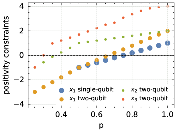
Figure 3: The maximal reachable positivity constraints $x_{l}$, corresponding to Eq. (48) and (59) of the erroneous state are presented as a function of the single- and two-qubit quantum state purity $p$. We assume that we have a systematic error of measuring ${\sigma_{\text{Y}}}$ instead of ${\sigma_{\text{Z}}}$ on one qubit. The black dashed line is located at a value of zero, and if a condition is $x_{l}$ is beyond that line, it means that there exists a quantum state with the respective purity which can detect the error. The minimal necessary state purity is $0.75$ and $0.3$ for single- and two-qubit states, respectively. The results for the single-qubit $x_{1}$ value begin from $0.5$, the purity of the maximally mixed state.

These results show that the minimum necessary purity for two-qubit states is significantly smaller than the one for single-qubit states. In particular, the results show that two-qubit quantum states are more sensitive to detect an error on a single-qubit Pauli measurement, due to the additional $\zeta_{2}$ and $\zeta_{3}$ positivity constraints of Eq. (58), which are violated already at a purity of $0.3$ and $0.4$, respectively. The single- and two-qubit $\zeta_{1}$ inequalities of Eq. (45) and (58) are violated at similar purity values around $0.7$, and this numerical values of the minimal necessary state purity agree with the results of presented in Fig. 1c, where the distance $D$ vanishes for states of having a purity below $0.75$. Of course, one has to keep in mind that purities of quantum states with a different number of qubits are sometimes difficult to compare.

B.3.2 Tensor Products with Single-Qubit State Copies

We have also studied if one can enhance the the single-qubit error detection capabilities by adding uncorrelated ancillas. We consider again the error of measuring $\sigma_{\operatorname{Y}}$ instead of $\sigma_{\operatorname{Z}}$ on the first qubit, and we use the true, underlying single-qubit state $\rho^{s}_{0.7}$ with purity of $0.7$, which maximizes the problem of Eq. (47). In particular, we consider three cases of tensor products. Firstly, we find that the tensor product of an erroneous state copy $\tilde{\rho}^{s}_{0.7}$ with a correct copy $\rho^{s}_{0.7}$ does not violate any positivity condition. Secondly, the same holds true for a tensor product of two copies of the erroneous state $\tilde{\rho}^{s}_{0.7}$. Finally, if we consider $\tilde{\rho}^{s}_{0.7}$ together with any eigenvector corresponding to the positive eigenvalue of $\sigma_{i}$, we only get a value of $0$ for the conditions $\zeta_{2}$ and $\zeta_{3}$. Table 1 summarizes the results for the $\zeta_{i}$ inequalities depending on the product state type. To sum up, these attempts to enhance the detection of a single qubit error merely by employing some tensor products in different cases have not been successful.

Table 1: Single-qubit error (${\sigma_{\text{Y}}}$ measurement for ${\sigma_{\text{Z}}}$) detection with several product states containing the erroneous single-qubit state $\tilde{\rho}^{s}_{0.7}$ with purity $0.7$.

product states	$\zeta_{1}$	$\zeta_{2}$	$\zeta_{3}$
$\tilde{\rho}^{s}_{0.7}\otimes\openone$	-0.20	-	-
$\tilde{\rho}^{s}_{0.7}\otimes\rho^{s}_{0.7}$	-1.480	-0.120	-0.014
$\tilde{\rho}^{s}_{0.7}\otimes\tilde{\rho}^{s}_{0.7}$	-0.760	-0.040	-0.002
$\tilde{\rho}^{s}_{0.7}\otimes(1,0,0)^{\operatorname{T}}$	-0.400	0	0

B.3.3 Entangled vs. Separable States in Error Detection Capability

In this subsection we address the question if there is a difference between product and entangled two-qubit states in the capability to detect local systematic errors on the first qubit. To have a severe systematic error on just one qubit is the most likely case, and thus we focus on this error. Our approach to this problem is to perform a brute force search over different angular configurations of the misalignment matrix $\operatorname{M}_{1}$. In particular, we vary both the Pauli $\operatorname{Y}$ and $\operatorname{Z}$ basis alignment of the first qubit in dependence of four angles $\alpha,\beta,\gamma,\delta$ as follows:

$$\operatorname{M}_{1}=\left(\begin{array}[]{lll}1&0&0\\ \sin{(\beta)}\sin{(\alpha)}&\cos{(\alpha)}&\cos{(\beta)}\sin{(\alpha)}\\ \sin{(\delta)}\sin{(\gamma)}&\cos{(\delta)}\sin{(\gamma)}&\cos{(\gamma)}\end{array}\right),$$ (68)

and we assume that there is no systematic error present on the second qubit, i.e., $\operatorname{M}_{2}=\openone$. It is straightforward to check that each row of the misalignment matrix above is normalized.

We check all permutations of the four angles for the interval $\{0,\frac{\pi}{8},\frac{\pi}{4},\frac{3\pi}{8},\frac{\pi}{2}\}$. For each angular setting we determine the values $x_{l}$ for the whole state space as given by Eq. (59) and for separable states as given by Eq. (64), where we vary the purity values beginning from $0.32$ to $0.38$. The optimization over the whole state space includes both entangled and separable states, whereas the optimization over the separable states includes only those, which enables us to compare entangled and separable states in their error detection capability.

We provide the Mathematica file from which we obtained the following results together with the numerical results and the plots generated from these results on reasonable request to JF. We have checked $625$ different angular settings, where $25$ of those angular settings correspond to having no error, because $\sin{(0)}$ terms in Eq. (68) ensure that we get the identity matrix. In summary, we have $600$ erroneous angular settings.

We find that the optimization problem returning the value $x_{3}$ is the most stringent condition, because it returns at smaller purity values already a positive value. We observe property of $x_{3}$ for all erroneous settings and for both entangled and separable states. Furthermore, we find that the first positive value of the conditions $x_{1}$ and $x_{2}$ strongly depends on the angular setting $\operatorname{M}_{1}$. However, the first positive value of $x_{3}$ is almost the same for all angular settings, which we find in the interval of the purity from $0.29$ to $0.34$, and $54\%$ of all erroneous settings return the smallest necessary state purity of $0.31$.

For most of the cases we find that the minimal necessary state purity is the same for entangled and separable states, just in some of these cases entangled states return larger values for $x_{l}$ than separable states for purity values beyond the minimal necessary state purity, which has been the same for both state types.

The only error setting for which entangled and product states differ drastically, is the one with the angular setting of $\alpha=\gamma=\frac{\pi}{2},\beta=\delta=0$, and this error corresponds to the permutation of the Pauli basis where the $\operatorname{Y}$ and $\operatorname{Z}$ are interpreted as $\operatorname{Z}$ and $\operatorname{Y}$, respectively, i.e.: $\operatorname{X}\mapsto\operatorname{X},\operatorname{Y}\mapsto\operatorname{Z},\operatorname{Z}\mapsto\operatorname{Y}$. In Fig. 4a-c we show the results $x_{l}$ of the optimization problems in Eq. (59) and Eq. (64) for entangled and separable states as blue and orange dots, respectively. The black dashed line is at $x_{l}=0$, and if a points above the line, it means that there exist a state that can detect the error. We find that only entangled states are able to detect this error, in particular, the blue dots in Fig. 4b and Fig. 4c are above the dashed line for purities beyond $0.45$ and $0.35$, respectively. On the other hand, the $x_{l}$ values for product states stay below or at the dashed line, which means that those are not able to detect the error.

The above mentioned error of permuting two bases corresponds to the partial transpose map together with an appropriate local unitary transformation. Thus, it is understandable that separable states are not able to detect those errors. From the above discussion the following question arises naturally: what happens if the adjustment angles are close to (but not exactly equal to) the partial transpose error? Is there still a difference between the entangled and separable states? To address this question, we have studied a partial transposition misalignment $M_{1}$ given by Eq. (68) with angles $\alpha=\gamma=\frac{\pi}{2}+\eta$ and $\beta=\delta=\eta$. Note that this error corresponds to exchanging the $Y$ and $Z$ basis, with a small angular offset of $\eta$ on each of the angles. We find for a value of $\eta=$0.05\text{\,}\mathrm{rad}$=$2.9\text{\,}\mathrm{\SIUnitSymbolDegree}$$ that again only entangled states violate the conditions $x_{2}$ and $x_{3}$ significantly as one can see in Fig. 5b-c. For separable states there is a violation, but it is much smaller and difficult to characterize experimentally. In this sense, entangled states can help to detect systematic errors.

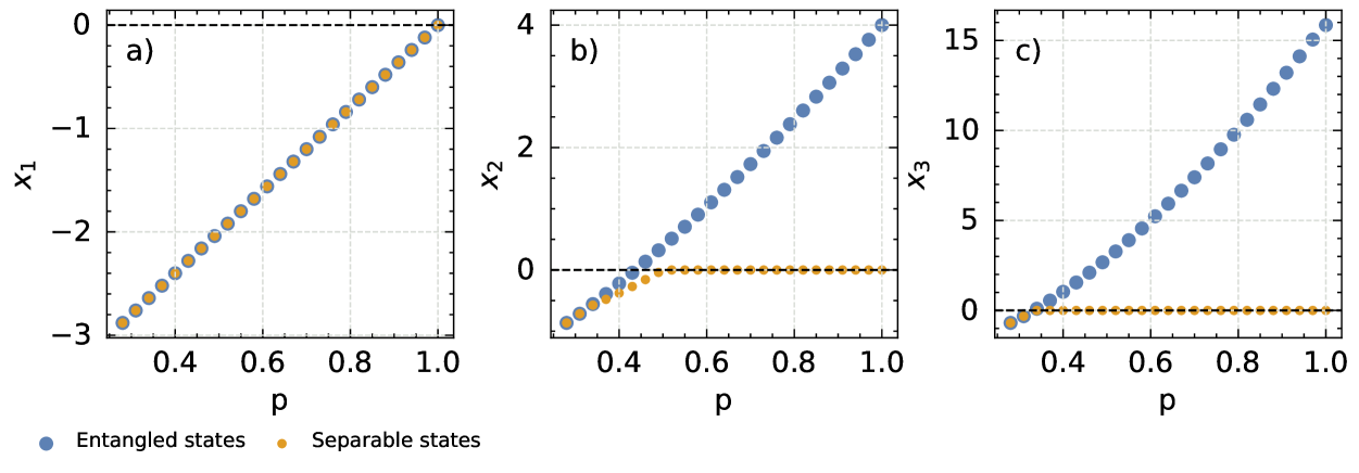
Figure 4: Numerical results for the maximal values of $x_{1}$ in a), $x_{2}$ in b) and $x_{3}$ in c) depending on the purity of the true, underlying two-qubit state $\rho$ for the error of interpreting the $\operatorname{Y}$ and $\operatorname{Z}$ as $\operatorname{Z}$ and $\operatorname{Y}$ Pauli measurement, respectively. The blue and orange dots represent the $x_{l}$ values for entangled and separable states from Eq. (59) and Eq. (64), respectively. If a point is above the black line at $x_{l}=0$, it means that one of the positivity constraints is violated, and thus, there exists at least one state that can detect the error. Only entangled states are able to detect this error by considering either the condition of $x_{2}$ or $x_{3}$, which returns values above the dashed line for purities beyond $0.45$ and $0.35$, respectively. The difference between the entangled and separable states comes from the fact that the considered measurement error is related to the partial transposition.

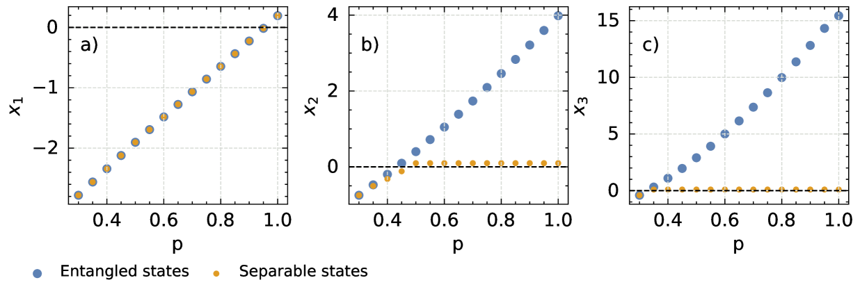
Figure 5: Numerical results for the maximal values of $x_{1}$ in a), $x_{2}$ in b) and $x_{3}$ in c) depending on the purity $p$ of the true, underlying two-qubit state $\rho$ for the misalignment $M_{1}$, Eq. (68), with angles $\alpha=\gamma=\frac{\pi}{2}+\eta$ and $\beta=\delta=\eta$. This error corresponds to exchanging the $\operatorname{Y}$ and $\operatorname{Z}$ basis, but with a small angular offset of $\eta=$0.05\text{\,}\mathrm{rad}$=$2.9\text{\,}\mathrm{\SIUnitSymbolDegree}$$. Again, the blue and orange dots represent the $x_{l}$ values for entangled and separable states from Eq. (59) and Eq. (64), respectively. The black dashed line is at values $x_{l}=0$, and it marks the threshold value for which the positivity constraint is violated and at least one state exists, which can detect the systematic error. The violations that can be reached with separable states are much smaller than the ones for entangled states, therefore entangled states can help in detecting this kind of error.

To conclude this section, we find that entangled states are able to detect more single-qubit errors than separable states, and we have discussed several example errors where this is the case. Furthermore, we find that for many error configurations entangled and separable states have the same minimal necessary state purity, and in some cases the actual numerical values of $x_{l}$ for entangled states are larger then those of separable states, but this happens only for state purities beyond the smallest necessary state purity.

B.4 n-Qubit Systems

Formally, our approach for determining the smallest necessary state purity to detect local errors, can be extended to a n-qubit system. The only fact one has to keep in mind is that the number of positivity conditions scales exponentially with the number of eigenvalues. At this point we leave the investigation of n-qubits for future work.

Appendix C Statistical and Systematic Error Distinction

In this section we utilize the vector Bernstein inequality from Ref. [27] to state a probability $\delta_{\text{sta}}$ that the distance $D$ between the least-squares and biased estimate, Eq. (3), is caused by statistical errors. In order to be able to use the vector Bernstein inequality, we have to reformulate the distance $D$ such that it contains the true, underlying quantum state $\rho$. The distance $D$ is the smallest distance between the least-squares estimator ${\rho_{\text{LS}}}$ and the physical state space, and thus, it is strictly smaller than the distance between the least-squares estimate and the true, underlying quantum state $\rho$: $D=\left\|{\rho_{\text{LS}}}-{\rho_{\text{B}}}\right\|_{2}\leq\left\|{\rho_{\text{LS}}}-\rho\right\|_{2}$. Furthermore, we interpret quantum state tomography as sum of independent, zero-mean, vector-valued random variables, where we define $\sigma$ as the average of the variances of the random variables. With this assumptions we utilize Eq. (A16) from Ref. [27], which makes us of the pseudo inverse map induced by Born’s rule ($\mathcal{A}:\rho\mapsto f$). Summarizing, we obtain the following bound on the probability $\delta_{\text{sta}}$ to observe statistical errors:

$$\delta_{\text{sta}} =\,\mathbb{P}\left[\left\|{\rho_{\text{LS}}}-{\rho_{\text{B}}}\right\|_{2}\geqslant\tau\right]\leq\mathbb{P}\left[\left\|{\rho_{\text{LS}}}-\rho\right\|_{2}\geqslant\tau\right]$$

$$\leq 8\exp\left[-\frac{N\tau^{2}}{2\sigma^{2}}\frac{3}{3+\sqrt{2}\tau/\sigma}\right],$$ (69)

where $\tau$ is a finite distance. For local Pauli measurements on $n$ qubits $\sigma$ is equal to $5^{n/2}$.

Appendix D Experimental Methods

D.1 Photon Source and Experimental Setup

A single GaAs/AlGaAs quantum dot (QD) embedded in a circular Bragg resonator cavity, also known as a bullseye cavity, serves as the source of entangled photons. The QD is a semiconductor nanostructure formed by tens of thousands of atoms, whose electronic structure features discrete energy levels due to quantum confinement. This is a distinctive feature of quantum emitters, namely light sources that rely on deterministic emission mechanisms and can produce photonic states with small multiphoton components [64]. The QD is fabricated by Al-droplet etching epitaxy, a technique that creates symmetric conical nanoholes in an $\text{Al}_{0.33}\text{Ga}_{0.67}\text{As}$ matrix, here about $7\text{\,}\mathrm{nm}$ in height and $50\text{\,}\mathrm{nm}$ in base diameter [65], that are filled with GaAs. The quantum dot is embedded in a photonic microcavity, here a circular Bragg resonator, that enhances photon extraction. The whole structure is sketched in Fig. 6a. More details on source fabrication and further micro-processing steps, in addition to the full sample design and optical performance, are described in reference [41].

Pairs of polarization-entangled photons are generated by the physical mechanism of the biexciton-exciton cascade, which is depicted in Fig. 6b. If two electron-hole pairs are confined in the quantum dot, a so-called biexciton state with total angular momentum $J=0$ along the quantization axis defined by the growth direction, is created. This excited state decays via spontaneous emission, a process that can follow two radiative paths based on the presence of two possible intermediate states, namely bright exciton states with different projections of the total angular momentum along the main confinement axis (superposition of $M_{z}=\pm 1$ states). The energy of the first optical transition (biexciton to exciton) is lower than the energy of the second transition (exciton to ground state) due to differences in Coulomb interaction in the excitonic states. Following the relevant optical selection rules, when the two decay paths are indistinguishable, that is when the two intermediate bright exciton states are degenerate, the two photons of the radiative cascade are emitted in the $\ket{\phi^{+}}=1/\sqrt{2}(\ket{HH}+\ket{VV})$ state of polarization [66].

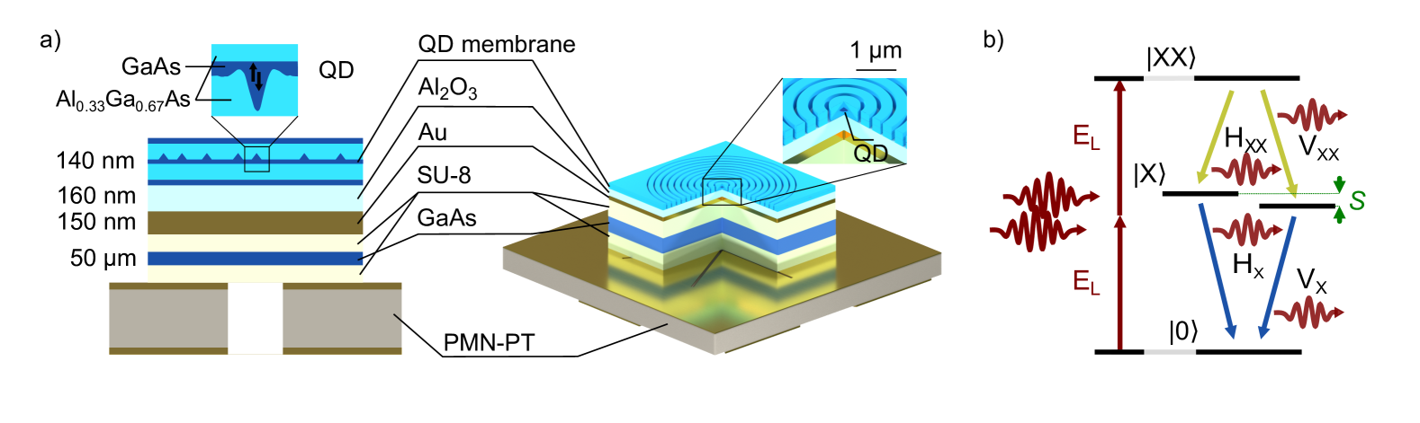
Figure 6: a) Sketch of the entangled photon source. A layer with GaAs QDs is fabricated via droplet etching epitaxy at the middle of a $140\,\text{nm}$ thick $\text{Al}_{0.33}\text{Ga}_{0.67}\text{As}$ membrane. The membrane is integrated on top of a micromachined piezoelectric substrate to induce controlled strain in the material. A circular Bragg grating microstructure is etched around a single QD to improve photon collection from above. b) Energy level picture of the biexciton-exciton radiative cascade that generates polarization-entangled photons. A fine structure splitting $S$ separates the two bright exciton states. A resonant two-photon absorption process directly populates the biexciton state.

Including non-idealities, the two-qubit density matrix that describes the polarization state of the two correlated photons depends on a few parameters (see also Appendix F.1). The main factor that influences the density matrix is the fine structure splitting, that is the energy splitting between the two intermediate bright-exciton states of the radiative cascade.

Fine-structure splitting introduces a phase in the entangled state that depends on the randomly distributed emission time of the exciton-to-ground state transition [67, 68]. Under the assumption of no spin dephasing processes, the state follows the following form: $\ket{\psi}=\frac{1}{\sqrt{2}}\left(\ket{HH}+e^{iE_{\text{FSS}}t/\hbar}\ket{VV}\right)$, where $E_{\text{FSS}}$ is the fine structure splitting and $t$ is the emission time of the exciton, where zero is the emission time of the biexciton. If the emission is time gated and the detector resolution is fast enough, this phase might be resolved, however, otherwise the phase evolution results in a mixed density matrix, which deviates from the dominant term $\ket{\phi^{+}}=\frac{1}{\sqrt{2}}\left(\ket{HH}+\ket{VV}\right)$. The amount of mixedness depends on the ratio between fine structure splitting and exciton recombination lifetime. Without the assumption of no spin dephasing, the state evolution can be found in matrix form in Appendix F. Here we control the fine structure splitting to modify the density matrix of the emitted two-photon states at a source level. Our entangled photon source is integrated on top of a micromachined piezoelectric substrate which allows us to induce a controlled strain and finely tune the value of fine structure splitting. In this experiment, the QD source is operated at three different levels of fine structure splitting, namely $0.6\text{\,}\mathrm{\SIUnitSymbolMicro eV}$ (negligible effect on the entanglement), $7.9\text{\,}\mathrm{\SIUnitSymbolMicro eV}$, and $13.9\text{\,}\mathrm{\SIUnitSymbolMicro eV}$. These three values of fine structure splitting correspond to a state purity of $0.92$, $0.65$, and $0.56$, in order. The lifetime is $93\text{\,}\mathrm{ps}$ and $42\text{\,}\mathrm{ps}$ for the exciton-to-ground-state and biexciton-to-exciton transition, respectively.

The photon source is cooled to $5\text{\,}\mathrm{K}$ inside a low-vibration closed-cycle He cryostat, where a single QD is optically excited by focusing laser light through a $0.81$ NA objective positioned within the cryostat in a confocal arrangement. The radiative cascade is prompted by populating the biexciton state of the QD via two-photon resonant excitation [69, 70]. The optical excitation is performed with a Ti:Sapphire pulsed laser with $80\text{\,}\mathrm{MHz}$ repetition rate. A 4f pulse shaper with an adjustable slit on its Fourier plane is used to select the laser energy at half the ground-to-biexciton state transition energy, enabling two-photon absorption, and at a bandwidth of $1060\text{\,}\mathrm{\SIUnitSymbolMicro eV}$, to minimize state mixing induced by laser-induced level shifts [71]. The power of the laser pulses is set at $\pi$-pulse of the Rabi oscillations, that is in the condition which maximizes brightness. To mitigate blinking, the QD charge environment is stabilized using an uncollimated halogen lamp with a blackbody spectrum [72]. The QD emits polarization-entangled photon pairs via the biexciton-exciton cascade. The two-qubit density matrix that describes the polarization state of the two correlated photons depends on a few parameters (see also Appendix F.1), including the fine structure splitting, that is the energy splitting between the two intermediate bright-exciton states of the radiative cascade. The effect of the fine structure splitting is to introduce a phase in the entangled state that depends on the randomly distributed emission time of the exciton-to-ground state transition [67, 68]. If the acquisition is not time gated, this results in a mixed density matrix with a dominant term due to the $\ket{\phi^{+}}=1/\sqrt{2}(\ket{HH}+\ket{VV})$ state and an additional contribution from the $\ket{\phi^{-}}=1/\sqrt{2}(\ket{HH}-\ket{VV})$ state, whose relative weight depends on the ratio between fine structure splitting and exciton recombination lifetime.

The light emitted by the QD is collected by the same objective used for optical excitation and separated from the excitation path using a 90:10 beam splitter. The backscattered laser light is suppressed using tunable volume Bragg gratings with a spectral bandwidth of $0.4\text{\,}\mathrm{nm}$. A second set of volume Bragg gratings, operated in reflection mode, is employed to spectrally separate the emission from the two optical transitions that are at $793.55\text{\,}\mathrm{nm}$ and $795.39\text{\,}\mathrm{nm}$. The quantum tomography setup consists of two sets of a half-wave plate and a quarter wave plate (for state rotation), a polarizing beam splitter (for state projection), and two silicon avalanche photodiodes. The quarter wave plate rotated by the additional angular offset $\Delta$ is in the analyzer of the photons from the biexciton-to-exciton transition. The detectors have a time jitter of approximately $400\text{\,}\mathrm{ps}$ (FWHM) and a detection efficiency of 46% including receptacle losses. The single-photon events are recorded using a time-to-digital converter from Swabian Instruments with a resolution of $10\text{\,}\mathrm{ps}$ (rms). Each two-qubit quantum state tomography is performed with two detectors per qubit in 9 different polarization settings, amounting to a total of 36 coincidence measurements [73]. The acquisition time for each polarization setting is $30\text{\,}\mathrm{s}$ at a coincidence rate of approximately 27 kcps.

D.2 Measurement Data Evaluation

We provide details on the evaluation of the measurement data shown in the main text to allow the interested reader to reconstruct the results from the given measurement data. We use two source codes, one to determine an array of coincidence events from the raw detector clicks and the other one to evaluate the estimators and their distance.

Table 2: Statistical properties for non-Gaussian histograms

$\Delta($\text{\,}\mathrm{\SIUnitSymbolDegree}$)$	mean $\mu$ in $10^{-3}$	standard deviation $\sigma$ in $10^{-3}$
50	0	1.5
60	5	5
130	0	0.5

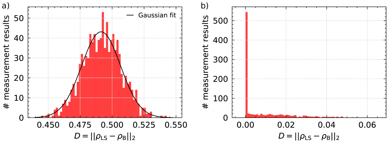
Figure 7: a) The histogram summarizes the determined distance $D(\Delta=$100\text{\,}\mathrm{\SIUnitSymbolDegree}$)$ for $1000$ sub-experiments for the state with the largest underlying state purity value ($0.6\text{\,}\mathrm{\SIUnitSymbolMicro eV}$ fine structure splitting). b) We observe for the state with the lowest purity that the resulting histogram for the distance $D(\Delta=$60\text{\,}\mathrm{\SIUnitSymbolDegree}$)$ exhibits a non-Gaussian statistical behavior. The reason for the enhancement of zero-distance bin is that the nonphysical state lies inside the physical state space, because the purity is so low that even with systematic error the nonphysical estimator is a physical state.

For the evaluation of the estimator distance, we divide the total measured coincidence counts for each basis setting in $N_{e}=1000$ sub experiments consisting of $N_{bs}=400$ coincidence events each. We split the array of measurement data in $N_{bs}=400$ blocks of size $N_{e}=1000$, whereas we assign each index in one block to one coincidence event of a sub-experiment. Subsequently, we evaluate for each sub-experiment the quantities of interest and bin the outcomes in a histogram.

Fig. 7a and Fig. 7b show the histograms with the results for the $D(\Delta=$100\text{\,}\mathrm{\SIUnitSymbolDegree}$)$ and $D(\Delta=$60\text{\,}\mathrm{\SIUnitSymbolDegree}$)$ measurement points of the states with the largest and smallest underlying purity, respectively. The resulting histogram of the high purity quantum state exhibits a Gaussian statistics as seen in Fig. 7a, and thus, we fit a Gaussian distribution over the histogram. We use the mean value and the standard deviation of the Gaussian distribution as the measurement result and its error in Fig. 2c of the main text, respectively.

For the low purity results we observe for some angles $\Delta$ an outcome distribution, which differs clearly from the Gaussian distribution, see Fig. 7b. We observe this outcome distributions because the purity is so low that most of the, though erroneous, unbiased estimates still result in a physical state, and thus, the zero distance bin is filled up with most of the measurement results. For these specific cases we do not fit a Gaussian distribution over the histogram. In particular, we sum over all histogram values beginning from $D=0$ until we reach a cumulative value of $68.2\%$ of the total measurement outcomes, and we define the mean value and its standard deviation as the central bin and half of the width of the interval containing $68.2\%$ of the data. The reason for taking $68.2\%$ is that it corresponds with the definition of the standard deviation for the Gaussian function. Table 2 contains all mean and standard deviation values for the low purity state with the offsets $\Delta$ for which the histogram is non-Gaussian.

D.2.1 Confidence regions for measurement data

In this section, we analyze the confidence region for the experiment described in the main text. The confidence level is defined as $1-\delta_{\text{sta}}$, where $\delta_{\text{sta}}$ represents the probability that the distance $D$ between the biased and unbiased estimators exceeds $\tau$ due to a systematic error. This probability is provided by Eq. 4 in the main text. In our experiment, we focus on a two-qubit state, meaning $n=2$, and we perform a total of $N=9\cdot 400$ measurements. Fig. 8 illustrates the confidence region as a function of $\tau$ from which we see that for a distance $\tau=0.25$ we get already a confidence level of $90\%$. Note that the bounds coming from the Bernstein inequality can get larger than $1$, which results in probabilities out of the interval $[0,1]$ and has been reported in the literature [74, 75]. Therefore, we adjust the probabilities in Fig. 8 when we observe values of $\tau$ below $0$.

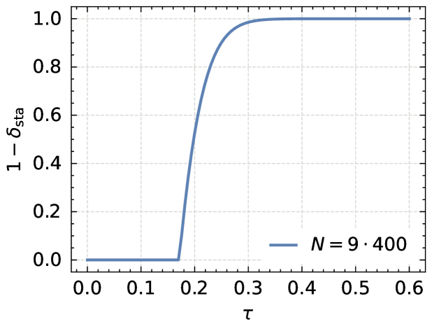
Figure 8: The confidence level $1-\delta_{\text{sta}}$ gives the probability that the distance between the estimators $D$ exceeds $\tau$ due to a systematic error for the experiment in the main text. We use Eq. 4 from the main text with the parameters $n=2$ and $N=9\cdot 400$ to obtain the confidence level as a function of $\tau$. We reach a confidence level of $90\%$ for a value of $\tau=0.25$.

Appendix E Quantum State Tomography of Qubits Implemented as the Polarization of Photons

Here, we review concisely how to implement local, single-qubit Pauli measurements of qubits, which are realized by the polarization of a photon. In particular, we discuss the how to implement single-qubit unitary operations with wave plates, and further, we discuss how Pauli measurements are implemented in those photonic systems.

E.1 Single-Qubit Unitary Operations

The implementation of unitary rotations of the photon’s polarization is crucial for the realization of local, single-qubit Pauli measurements. In our work we use quarter- and half-wave plates to perform unitary rotations on the photon’s polarization, thus we summarize briefly the matrix formalism to treat wave plates, following the book of Pedrotti et al. [76]. A wave plate is an optical component (often cutout from a birefringent crystal), which causes an additional phase shifts for both the horizontal $\ket{H}$ and vertical $\ket{V}$ component of the photon’s polarisation. The most general form of a wave plate $\operatorname{W}$ is given by the following matrix,

$$\operatorname{W}=\left(\begin{array}[]{ll}e^{\mathrm{i}\varepsilon_{x}}&0\\ 0&e^{\mathrm{i}\varepsilon_{y}}\end{array}\right)=e^{\mathrm{i}\varepsilon_{H}}\left(\begin{array}[]{ll}1&0\\ 0&e^{\mathrm{i}(\varepsilon_{V}-\varepsilon_{H})}\end{array}\right),$$ (70)

where $\varepsilon_{H}$ and $\varepsilon_{V}$ represent the phase change shift of the $H$ and $V$ component of the polarization. A quarter wave plate with fast axis vertically aligned, i.e. perpendicular to both the optical table and the photon’s propagation direction, is obtained from Eq. (70) for phase shift of $\pi/4$ and $-\pi/4$ for the horizontal and vertical polarization component:

$$\operatorname{U}_{\mathrm{QWP,FAV}}=e^{\mathrm{i}\pi/4}\left(\begin{array}[]{cc}1&0\\ 0&-\mathrm{i}\end{array}\right).$$ (73)

Note that the matrix in Eq. (73) is the $\operatorname{S}^{\dagger}$ gate. If the fast axis of the quarter wave plate is oriented horizontally, i.e., parallel to the optical table, the representing matrix differs from Eq. (73) in terms of the sign of the relative and absolute phase,

$$\operatorname{U}_{\mathrm{QWP,FAH}}=e^{-\mathrm{i}\pi/4}\left(\begin{array}[]{ll}1&0\\ 0&\mathrm{i}\end{array}\right).$$ (74)

The matrix representation of a half-wave plate with fast axis oriented vertical is given as follows,

$$\operatorname{U}_{\mathrm{HWP,FAV}}=e^{\mathrm{i}\pi/2}\left(\begin{array}[]{cc}1&0\\ 0&-1\end{array}\right).$$ (77)

A half-wave plate with fast axis oriented horizontal is described by the same matrix as in Eq. (77), merely the sign of the absolute phase term is opposite. Note that the matrix, Eq. (77), corresponds to the $\operatorname{Z}$ gate.

E.2 Single-Qubit Pauli Basis Measurements

The photonic system we consider utilizes the polarization of a photon to implement the basis states of a qubit. Therefore, a computational basis measurement (${\sigma_{\text{Z}}}$ measurement) is implemented by observing clicks on a single-photon detector on each exit of a polarizing beam splitter (PBS). The remaining Pauli measurements are performed by inserting a quarter and half-wave plate prior to the PBS, see Fig. 2b in the main text for a visualization of the measurement setup. The fast axis rotation angles $\psi_{k}$ and $\chi_{k}$ for the quarter and half-wave plate are determined from the expectation values of the $k$-th Pauli measurement setting as follows:

$${\operatorname{Tr}}\left(\sigma_{k}\rho\right)={\operatorname{Tr}}\left(\operatorname{R^{\text{rot}}}\left(\chi_{k}\right){\sigma_{\text{Z}}}\operatorname{R^{\text{rot}}}\left(-\chi_{k}\right)\operatorname{R^{\text{rot}}}\left(\psi_{k}\right)\operatorname{S}\operatorname{R^{\text{rot}}}\left(-\psi_{k}\right){\sigma_{\text{Z}}}\operatorname{R^{\text{rot}}}\left(\psi_{k}\right)\operatorname{S}^{\dagger}\operatorname{R^{\text{rot}}}\left(-\psi_{k}\right)\operatorname{R^{\text{rot}}}\left(\chi_{k}\right){\sigma_{\text{Z}}}^{\dagger}\operatorname{R^{\text{rot}}}\left(-\chi_{k}\right)\rho\right),$$ (78)

where $k\in\{1,\dots N_{\text{b}}\}$ is one of the $N_{\text{b}}$ measurement basis settings, and $\operatorname{R^{\text{rot}}}$ is the rotation matrix:

$$\operatorname{R^{\text{rot}}}(\theta)=\left(\begin{array}[]{cc}\cos(\theta)&-\sin(\theta)\\ \sin(\theta)&\cos(\theta)\\ \end{array}\right).$$ (81)

We summarize the rotation angles for the Pauli basis measurements in Table 3.

Table 3: Pauli measurement angles

Pauli basis	$\psi$	$\chi$
${\sigma_{\text{X}}}$	$0$	$\frac{\pi}{8}$
${\sigma_{\text{Y}}}$	$\frac{\pi}{4}$	$0$
${\sigma_{\text{Z}}}$	$0$	$0$

Appendix F Experimental Errors With Polarization-Entangled Photon Pairs

In this section we provide a non-exhaustive list of possible errors in a quantum optics lab, where the photon’s polarization defines the qubit and local, single-qubit Pauli basis measurements are performed with wave plates and beam splitters. For other qubit implementations [77] and optical components, as for example electro-optic modulators [78], other error settings may occur.

F.1 Rotation of a Single Pauli Basis

In the main text, we present the single-qubit case with a misalignment of a single Pauli basis. Here, we simulate two-qubit quantum states of varying purity emitted by quantum dots. Ideally, the emitted quantum state from a quantum dot is the Bell state $\ket{\phi^{+}}$, but fine structure splitting and the finite lifetimes of the exciton lead to a state deviating from $|\phi^{+}\rangle$. We use the model proposed by Hudson et al. [79] to describe a plausible quantum state $\rho$ generated by a quantum dot:

$$\rho=\frac{1}{4}\left(\begin{array}[]{cccc}1+\kappa g_{H,V}^{\prime(1)}&0&0&2\kappa g_{H,V}^{(1)}z^{*}\\ 0&1-\kappa g_{H,V}^{\prime(1)}&0&0\\ 0&0&1-\kappa g_{H,V}^{\prime(1)}&0\\ 2\kappa g_{H,V}^{(1)}z&0&0&1+\kappa g_{H,V}^{\prime(1)}\end{array}\right)$$ (82)

with

$$g_{H,V}^{\prime(1)}=1/\left(1+\tau_{1}/\tau_{SS}\right),$$

$$g_{H,V}^{(1)}=1/\left(1+\tau_{1}/\tau_{SS}+\tau_{1}/\tau_{HV}\right),$$

$$z=\frac{1+\mathrm{i}\iota}{1+\iota^{2}}\quad\text{and}\quad\iota=\frac{g_{H,V}^{(1)}S\tau_{1}}{\hbar}.$$ (83)

In this simulation we set the lifetime of the exciton $\tau_{1}=$150\text{\,}\mathrm{ps}$$, and the fraction of photon pairs originating exclusively from the quantum dot $\kappa=0.02$. We consider spin scattering and cross dephasing negligible by setting $\tau_{\mathrm{SS}}=$1\text{\,}\mathrm{\SIUnitSymbolMicro s}$$ and $\tau_{\text{HV}}=$1\text{\,}\mathrm{\SIUnitSymbolMicro s}$$. We vary the fine structure splitting from $0$ to $10\text{\,}\mathrm{\SIUnitSymbolMicro eV}$, which results in quantum states with purity ranging from $0.92$ to $0.58$, as in the experiment reported in the main text.

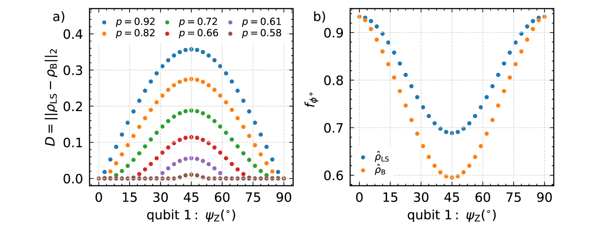
Figure 9: a) Distance $D$ as a function of rotation angle $\psi_{\text{Z}}$ of the quarter wave plate on qubit 1 for six different two-qubit state purities, ranging from $0.58$ to $0.92$. The rotation effects the basis terms: ${\sigma_{\text{Z}}}\otimes{\sigma_{\text{X}}}$, ${\sigma_{\text{Z}}}\otimes{\sigma_{\text{Y}}}$ and ${\sigma_{\text{Z}}}\otimes{\sigma_{\text{Z}}}$. The maximum $D$ is found for an angle $\psi_{\text{Z}}=$45\text{\,}\mathrm{\SIUnitSymbolDegree}$$, where ${\sigma_{\text{Y}}}$ is measured for ${\sigma_{\text{Z}}}$. The distance $D$ decreases for decreasing state purities. b) Fidelity w.r.t $|\phi^{+}\rangle$ evaluated for the least-squares estimator ${\rho_{\text{LS}}}$ (blue) and biased estimator ${\rho_{\text{B}}}$ (orange) depending on the rotation $\psi^{\text{Z}}$ of the quarter wave plate at qubit 1. The estimators are obtained from the measurement of the state with purity $0.92$. The fidelity values differ as function of the rotation angle and have a maximum at $\psi^{\text{Z}}=$45\text{\,}\mathrm{\SIUnitSymbolDegree}$$ where ${\sigma_{\text{Y}}}$ is measured instead of ${\sigma_{\text{Z}}}$.

We perform local, single-qubit Pauli measurements $\operatorname{P}_{\mathrm{qb1}}\otimes\operatorname{P}_{\mathrm{qb0}}$ with a fixed sequence of basis measurements: ${\sigma_{\text{X}}}\otimes{\sigma_{\text{X}}}$, ${\sigma_{\text{X}}}\otimes{\sigma_{\text{Y}}}$,…${\sigma_{\text{Z}}}\otimes{\sigma_{\text{Y}}}$,${\sigma_{\text{Z}}}\otimes{\sigma_{\text{Z}}}$ applied to qubit 1 and 0, respectively, such that the number of wave plate rotations is minimal. We assume that an error occurs during the adjustment of the ${\sigma_{\text{Z}}}$ basis on qubit 1, which implies effects on the three basis measurements: ${\sigma_{\text{Z}}}\otimes{\sigma_{\text{X}}}$,${\sigma_{\text{Z}}}\otimes{\sigma_{\text{Y}}}$ and ${\sigma_{\text{Z}}}\otimes{\sigma_{\text{Z}}}$. Fig. 9a shows the distance $D$ as function of the angle $\psi_{\text{Z}}$ on qubit 1 for quantum states with a purity ranging from $0.58$ to $0.92$. The maximum of the distance $D$ is found for the angle $\psi_{\text{Z}}=$45\text{\,}\mathrm{\SIUnitSymbolDegree}$$, this corresponds to the case of measuring ${\sigma_{\text{Y}}}$ instead of ${\sigma_{\text{Z}}}$. Furthermore, we see that the magnitude of the distance $D$ decreases for decreasing values of the state purity, as discussed in the main text.

Fig. 9b shows the fidelity with respect to the Bell state $\ket{\phi^{+}}$ for the estimators ${\rho_{\text{LS}}}$ (blue) and ${\rho_{\text{B}}}$ (orange) as function of the angle $\psi_{\text{Z}}$ on qubit 1. Both types of estimators have been obtained from the measured quantum state with purity $0.92$. The resulting fidelity for the physical and nonphysical estimator differs from each other as function of $\psi_{\text{Z}}$. The maximal difference in fidelity is obtained for $\psi_{\text{Z}}=$45\text{\,}\mathrm{\SIUnitSymbolDegree}$$, where ${\sigma_{\text{Y}}}$ is measured instead of ${\sigma_{\text{Z}}}$.

F.2 Exchange of wave plate Sequence

Here, we consider the unintended exchange of the quarter and half-wave plate in the measurement setup of Fig. 2b. We assume that the wave plates are perfectly aligned and the angles are adjusted as given in Table 3. Mathematically, this error corresponds to exchanging the ${\sigma_{\text{Z}}}({\sigma_{\text{Z}}}^{\dagger})$ and $\operatorname{S}^{\dagger}(\operatorname{S})$ between the rotation matrices $\operatorname{R}(\psi_{i})$ and $\operatorname{R}(\chi_{i})$ in Eq. (78), respectively. This error case has an effect on the implementation of the ${\sigma_{\text{X}}}$ and ${\sigma_{\text{Y}}}$ basis,

$$\sigma_{\mathrm{X,error}}=\frac{1}{2}\left(\begin{array}[]{cc}1&1+\mathrm{i}\\ 1-\mathrm{i}&-1\\ \end{array}\right)={\sigma_{\text{X}}}-{\sigma_{\text{Y}}}+{\sigma_{\text{Z}}}$$ (86)

$$\sigma_{\mathrm{Y,error}}=-{\sigma_{\text{Z}}}=-\left(\begin{array}[]{cc}1&0\\ 0&-1\\ \end{array}\right).$$ (89)

These errors caused on the ${\sigma_{\text{X}}}$ and ${\sigma_{\text{Y}}}$ measurement are detectable under as discussed in Appendix B.

F.3 Misalignment of the Quarter Wave Plate’s Fast Axis

Here, we discuss the cases of the unintended horizontal instead of vertical alignment of the quarter wave plate’s fast axis, this exchange corresponds to the use of matrix Eq. (74) instead of Eq. (73) for the Pauli measurements. The same misalignment of the half-wave plate’s fast axis causes no problems, because the resulting matrix Eq. (77) is up to a global phase factor the same for vertical and horizontal orientation of the fast axis. Mathematically, the horizontal orientation of the quarter wave plate corresponds to exchanging the $\operatorname{S}^{\dagger}$ and $(\operatorname{S})$ gate in Eq. (78), which effects the ${\sigma_{\text{Y}}}$ basis measurement as follows,

$$\sigma_{\mathrm{Y,error}}=-{\sigma_{\text{Y}}},$$ (90)

and this error corresponds performing a transposition of the single-qubit or a partial transpositon of the two-qubit quantum state, respectively. This error is not detectable, if we only have a single-qubit state or a two-qubit state product state. But as soon as the two-qubit state is entangled, we are able to detect this error as we have demonstrated in the main text and in Appendix B.3.3.

F.4 Further Errors

For the sake of completeness, we mention briefly other possibilities for errors and provide references to works considering these errors in detail.

The wave plates used in the Pauli basis measurement, can lead to errors effecting the matrices in Eqs. (73, 74, 77) of the quarter and half-wave plates, which may result in nonphysical quantum state estimates. West and Smith [80] discuss polarization errors for zero-order wave plates caused by thickness mismatch, optical axis tilt and fast axis misalignment of the two crystals used in the wave plate. The polarization error caused by the light’s incidence angle is discussed as well by West and Smith. Boulbry et al. [81] discuss the emerging of elliptical eigenpolarization modes caused by the misalignment of the optical axis a double crystal, achromatic, zero-order quarter wave plate.

Altepeter et al. [61] provide an extensive discussion on errors of photonic polarization qubit measurements and how to correct them. They discuss errors caused by the crosstalk and absorption of the polarizing beam splitter as well as the effect of the efficiency mismatches of the two single-photon detectors used at the two beam splitter exits.

References

- Nielsen and Chuang [2010] M. A. Nielsen and I. L. Chuang, Quantum Computation and Quantum Information: 10th Anniversary Edition (Cambridge University Press, 2010).
- Horodecki [2021] R. Horodecki, Quantum information, Acta Physica Polonica A 139, 197 (2021).
- Zoller et al. [2005] P. Zoller, T. Beth, D. Binosi, R. Blatt, H. Briegel, D. Bruss, T. Calarco, J. I. Cirac, D. Deutsch, J. Eisert, et al., Quantum information processing and communication, The European Physical Journal D - Atomic, Molecular, Optical and Plasma Physics 36, 203 (2005).
- Chen [2021] J. Chen, Review on quantum communication and quantum computation, Journal of Physics: Conference Series 1865, 022008 (2021).
- Wehner et al. [2018] S. Wehner, D. Elkouss, and R. Hanson, Quantum internet: A vision for the road ahead, Science 362, eaam9288 (2018).
- Foreman et al. [2023] C. Foreman, S. Wright, A. Edgington, M. Berta, and F. J. Curchod, Practical randomness amplification and privatisation with implementations on quantum computers, Quantum 7, 969 (2023).
- Dalzell et al. [2023] A. M. Dalzell, S. McArdle, M. Berta, P. Bienias, C.-F. Chen, A. Gilyén, C. T. Hann, M. J. Kastoryano, E. T. Khabiboulline, A. Kubica, G. Salton, S. Wang, and F. G. S. L. Brandão, Quantum algorithms: A survey of applications and end-to-end complexities (2023), arXiv:2310.03011 [quant-ph] .
- Harrow and Montanaro [2017] A. W. Harrow and A. Montanaro, Quantum computational supremacy, Nature 549, 203 (2017).
- Fauseweh [2024] B. Fauseweh, Quantum many-body simulations on digital quantum computers: State-of-the-art and future challenges, Nature Communications 15, 2123 (2024).
- Buluta and Nori [2009] I. Buluta and F. Nori, Quantum simulators, Science 326, 108 (2009).
- Houck et al. [2012] A. A. Houck, H. E. Türeci, and J. Koch, On-chip quantum simulation with superconducting circuits, Nature Physics 8, 292 (2012).
- Aspuru-Guzik and Walther [2012] A. Aspuru-Guzik and P. Walther, Photonic quantum simulators, Nature Physics 8, 285 (2012).
- Paris and Rehacek [2004] M. Paris and J. Rehacek, Quantum state estimation, Vol. 649 (Springer Science & Business Media, 2004).
- Huang et al. [2020] H.-Y. Huang, R. Kueng, and J. Preskill, Predicting many properties of a quantum system from very few measurements, Nature Physics 16, 1050 (2020).
- Nguyen et al. [2022] H. C. Nguyen, J. L. Bönsel, J. Steinberg, and O. Gühne, Optimizing shadow tomography with generalized measurements, Physical Review Letters 129, 220502 (2022).
- Moroder and Gittsovich [2012] T. Moroder and O. Gittsovich, Calibration-robust entanglement detection beyond Bell inequalities, Physical Review A 85, 032301 (2012).
- Tavakoli [2021] A. Tavakoli, Semi-device-independent framework based on restricted distrust in prepare-and-measure experiments, Physical Review Letters 126, 210503 (2021).
- Cao et al. [2024] H. Cao, S. Morelli, L. A. Rozema, C. Zhang, A. Tavakoli, and P. Walther, Genuine multipartite entanglement detection with imperfect measurements: Concept and experiment, Phys. Rev. Lett. 133, 150201 (2024).
- Svegborn et al. [2025] E. Svegborn, N. d’Alessandro, O. Gühne, and A. Tavakoli, Imprecision plateaus in quantum steering, Phys. Rev. A 111, L020404 (2025).
- Cieśliński et al. [2024] P. Cieśliński, J. Dziewior, L. Knips, W. Kłobus, J. Meinecke, T. Paterek, H. Weinfurter, and W. Laskowski, Valid and efficient entanglement verification with finite copies of a quantum state, npj Quantum Information 10, 14 (2024).
- Wölk et al. [2019] S. Wölk, T. Sriarunothai, G. S. Giri, and C. Wunderlich, Distinguishing between statistical and systematic errors in quantum process tomography, New Journal of Physics 21, 013015 (2019).
- Christandl and Renner [2012] M. Christandl and R. Renner, Reliable quantum state tomography, Physical Review Letters 109, 120403 (2012).
- Sugiyama et al. [2012] T. Sugiyama, P. S. Turner, and M. Murao, Effect of non-negativity on estimation errors in one-qubit state tomography with finite data, New Journal of Physics 14, 085005 (2012).
- Wang et al. [2019] J. Wang, V. B. Scholz, and R. Renner, Confidence polytopes in quantum state tomography, Physical Review Letters 122, 190401 (2019).
- Faist and Renner [2016] P. Faist and R. Renner, Practical and reliable error bars in quantum tomography, Physical Review Letters 117, 010404 (2016).
- Guţă et al. [2020] M. Guţă, J. Kahn, R. Kueng, and J. A. Tropp, Fast state tomography with optimal error bounds, Journal of Physics A: Mathematical and Theoretical 53, 204001 (2020).
- de Gois and Kleinmann [2024] C. de Gois and M. Kleinmann, User-friendly confidence regions for quantum state tomography, Physical Review A 109, 062417 (2024).
- Yu et al. [2022] X. Yu, J. Shang, and O. Gühne, Statistical methods for quantum state verification and fidelity estimation, Advanced Quantum Technologies 5, 2100126 (2022).
- Knips et al. [2015] L. Knips, C. Schwemmer, N. Klein, J. Reuter, G. Tóth, and H. Weinfurter, How long does it take to obtain a physical density matrix? (2015), arXiv:1512.06866 [quant-ph] .
- Rosset et al. [2012] D. Rosset, R. Ferretti-Schöbitz, J.-D. Bancal, N. Gisin, and Y.-C. Liang, Imperfect measurement settings: Implications for quantum state tomography and entanglement witnesses, Physical Review A 86, 062325 (2012).
- Schwemmer et al. [2015] C. Schwemmer, L. Knips, D. Richart, H. Weinfurter, T. Moroder, M. Kleinmann, and O. Gühne, Systematic errors in current quantum state tomography tools, Physical Review Letters 114, 080403 (2015).
- Silva et al. [2017] G. B. Silva, S. Glancy, and H. M. Vasconcelos, Investigating bias in maximum-likelihood quantum-state tomography, Physical Review A 95, 022107 (2017).
- Miranowicz et al. [2014] A. Miranowicz, K. Bartkiewicz, J. Peřina, M. Koashi, N. Imoto, and F. Nori, Optimal two-qubit tomography based on local and global measurements: Maximal robustness against errors as described by condition numbers, Physical Review A 90, 062123 (2014).
- Wang et al. [2023] J. Wang, S. Zhang, J. Cai, Z. Liao, C. Arenz, and R. Betzholz, Robustness of random-control quantum-state tomography, Physical Review A 108, 022408 (2023).
- Ivanova-Rohling et al. [2023] V. N. Ivanova-Rohling, N. Rohling, and G. Burkard, Optimal quantum state tomography with noisy gates, EPJ Quantum Technology 10, 25 (2023).
- Feito et al. [2009] A. Feito, J. S. Lundeen, H. Coldenstrodt-Ronge, J. Eisert, M. B. Plenio, and I. A. Walmsley, Measuring measurement: theory and practice, New Journal of Physics 11, 093038 (2009).
- Novik [2019] P. I. Novik, Diagnostics of systematic errors during single-photon detector operation, Journal of Applied Spectroscopy 86, 802 (2019).
- Moroder et al. [2013] T. Moroder, M. Kleinmann, P. Schindler, T. Monz, O. Gühne, and R. Blatt, Certifying systematic errors in quantum experiments, Physical Review Letters 110, 180401 (2013).
- Langford [2013] N. K. Langford, Errors in quantum tomography: diagnosing systematic versus statistical errors, New Journal of Physics 15, 035003 (2013).
- Schimpf et al. [2021] C. Schimpf, M. Reindl, F. Basso Basset, K. D. Jöns, R. Trotta, and A. Rastelli, Quantum dots as potential sources of strongly entangled photons: Perspectives and challenges for applications in quantum networks, Applied Physics Letters 118, 100502 (2021).
- Rota et al. [2024] M. B. Rota, T. M. Krieger, Q. Buchinger, M. Beccaceci, J. Neuwirth, H. Huet, N. Horová, G. Lovicu, G. Ronco, S. F. Covre da Silva, et al., A source of entangled photons based on a cavity-enhanced and strain-tuned GaAs quantum dot, eLight 4, 13 (2024).
- Trotta et al. [2015] R. Trotta, J. Martín-Sánchez, I. Daruka, C. Ortix, and A. Rastelli, Energy-tunable sources of entangled photons: A viable concept for solid-state-based quantum relays, Physical Review Letters 114, 150502 (2015).
- James et al. [2001] D. F. V. James, P. G. Kwiat, W. J. Munro, and A. G. White, Measurement of qubits, Physical Review A 64, 052312 (2001).
- Řeháček et al. [2004] J. Řeháček, B.-G. Englert, and D. Kaszlikowski, Minimal qubit tomography, Physical Review A 70, 052321 (2004).
- Teo et al. [2010] Y. S. Teo, H. Zhu, and B.-G. Englert, Product measurements and fully symmetric measurements in qubit-pair tomography: A numerical study, Optics Communications 283, 724–729 (2010).
- Zhu and Englert [2011] H. Zhu and B.-G. Englert, Quantum state tomography with fully symmetric measurements and product measurements, Physical Review A 84, 022327 (2011).
- Stricker et al. [2022] R. Stricker, M. Meth, L. Postler, C. Edmunds, C. Ferrie, R. Blatt, P. Schindler, T. Monz, R. Kueng, and M. Ringbauer, Experimental single-setting quantum state tomography, PRX Quantum 3, 040310 (2022).
- Jung et al. [2024] D. Jung, Y.-W. Cho, Y. Kim, and J. Lee, Coarse-grained quantum state tomography with optimal POVM construction (2024), arXiv:2404.06285 [quant-ph] .
- Neuwirth et al. [2022] J. Neuwirth, F. Basso Basset, M. B. Rota, J.-G. Hartel, M. Sartison, S. F. Covre da Silva, K. D. Jöns, A. Rastelli, and R. Trotta, Multipair-free source of entangled photons in the solid state, Physical Review B 106, L241402 (2022).
- Kimura [2003] G. Kimura, The Bloch vector for n-level systems, Physics Letters A 314, 339 (2003).
- Gamel [2016] O. Gamel, Entangled Bloch spheres: Bloch matrix and two-qubit state space, Physical Review A 93, 062320 (2016).
- da Silva et al. [2021] S. F. C. da Silva, G. Undeutsch, B. Lehner, S. Manna, T. M. Krieger, M. Reindl, C. Schimpf, R. Trotta, and A. Rastelli, GaAs quantum dots grown by droplet etching epitaxy as quantum light sources, Applied Physics Letters 119, 120502 (2021).
- Moore [1920] E. H. Moore, On the reciprocal of the general algebraic matrix, Bulletin of American Mathematical Society 26, 394 (1920).
- Penrose [1955] R. Penrose, A generalized inverse for matrices, Mathematical Proceedings of the Cambridge Philosophical Society 51, 406–413 (1955).
- Smolin et al. [2012] J. A. Smolin, J. M. Gambetta, and G. Smith, Efficient method for computing the maximum-likelihood quantum state from measurements with additive Gaussian noise, Physical Review Letters 108, 070502 (2012).
- Diamond and Boyd [2016] S. Diamond and S. Boyd, CVXPY: A Python-embedded modeling language for convex optimization, Journal of Machine Learning Research 17, 1 (2016).
- Agrawal et al. [2018] A. Agrawal, R. Verschueren, S. Diamond, and S. Boyd, A rewriting system for convex optimization problems, Journal of Control and Decision 5, 42 (2018).
- Hradil [1997] Z. Hradil, Quantum-state estimation, Physical Review A 55, R1561 (1997).
- Blume-Kohout [2010] R. Blume-Kohout, Optimal, reliable estimation of quantum states, New Journal of Physics 12, 043034 (2010).
- Press et al. [1988] W. H. Press, W. T. Vetterling, S. A. Teukolsky, and B. P. Flannery, Numerical recipes (Citeseer, 1988).
- Altepeter et al. [2005a] J. Altepeter, E. Jeffrey, and P. Kwiat, Photonic state tomography (Academic Press, 2005) pp. 105–159.
- Peres [1996] A. Peres, Separability criterion for density matrices, Physical Review Letters 77, 1413 (1996).
- Horodecki et al. [1996] M. Horodecki, P. Horodecki, and R. Horodecki, Separability of mixed states: necessary and sufficient conditions, Physics Letters A 223, 1 (1996).
- Hanschke et al. [2018] L. Hanschke, K. A. Fischer, S. Appel, D. Lukin, J. Wierzbowski, S. Sun, R. Trivedi, J. Vučković, J. J. Finley, and K. Müller, Quantum dot single-photon sources with ultra-low multi-photon probability, npj Quantum Information 4, 43 (2018).
- Huo et al. [2013] Y. Huo, A. Rastelli, and O. Schmidt, Ultra-small excitonic fine structure splitting in highly symmetric quantum dots on GaAs (001) substrate, Applied Physics Letters 102, 10.1063/1.4802088 (2013).
- Benson et al. [2000] O. Benson, C. Santori, M. Pelton, and Y. Yamamoto, Regulated and entangled photons from a single quantum dot, Phys. Rev. Lett. 84, 2513 (2000).
- Hudson et al. [2007a] A. J. Hudson, R. M. Stevenson, A. J. Bennett, R. J. Young, C. A. Nicoll, P. Atkinson, K. Cooper, D. A. Ritchie, and A. J. Shields, Coherence of an entangled exciton-photon state, Phys. Rev. Lett. 99, 266802 (2007a).
- Rota et al. [2020] M. B. Rota, F. B. Basset, D. Tedeschi, and R. Trotta, Entanglement teleportation with photons from quantum dots: Toward a solid-state based quantum network, IEEE Journal of Selected Topics in Quantum Electronics 26, 1 (2020).
- Jayakumar et al. [2013] H. Jayakumar, A. Predojević, T. Huber, T. Kauten, G. S. Solomon, and G. Weihs, Deterministic photon pairs and coherent optical control of a single quantum dot, Phys. Rev. Lett. 110, 135505 (2013).
- Müller et al. [2014] M. Müller, S. Bounouar, K. D. Jöns, M. Glässl, and P. Michler, On-demand generation of indistinguishable polarization-entangled photon pairs, Nature Photonics 8, 224 (2014).
- Basso Basset et al. [2023] F. Basso Basset, M. B. Rota, M. Beccaceci, T. M. Krieger, Q. Buchinger, J. Neuwirth, H. Huet, S. Stroj, S. F. Covre da Silva, G. Ronco, C. Schimpf, S. Höfling, T. Huber-Loyola, A. Rastelli, and R. Trotta, Signatures of the optical stark effect on entangled photon pairs from resonantly pumped quantum dots, Phys. Rev. Lett. 131, 166901 (2023).
- Nguyen et al. [2013] H. S. Nguyen, G. Sallen, M. Abbarchi, R. Ferreira, C. Voisin, P. Roussignol, G. Cassabois, and C. Diederichs, Photoneutralization and slow capture of carriers in quantum dots probed by resonant excitation spectroscopy, Phys. Rev. B 87, 115305 (2013).
- Altepeter et al. [2005b] J. B. Altepeter, E. R. Jeffrey, P. G. Kwiat, S. Tanzilli, N. Gisin, and A. Acín, Experimental methods for detecting entanglement, Phys. Rev. Lett. 95, 033601 (2005b).
- Tropp [2015] J. A. Tropp, An introduction to matrix concentration inequalities, Foundations and Trends® in Machine Learning 8, 1 (2015).
- Gross et al. [2010] D. Gross, Y.-K. Liu, S. T. Flammia, S. Becker, and J. Eisert, Quantum state tomography via compressed sensing, Phys. Rev. Lett. 105, 150401 (2010).
- Pedrotti et al. [2007] F. L. Pedrotti, L. M. Pedrotti, and L. S. Pedrotti, Introduction to Optics, 3rd ed. (Pearson Addison Wesley, San Francisco, 2007) Chap. 14.
- Brendel et al. [1999] J. Brendel, N. Gisin, W. Tittel, and H. Zbinden, Pulsed energy-time entangled twin-photon source for quantum communication, Physical Review Letters 82, 2594 (1999).
- Lo et al. [2019] H.-P. Lo, T. Ikuta, N. Matsuda, T. Honjo, and H. Takesue, Electro-optic modulators for photonic quantum information processing, in Quantum and Nonlinear Optics VI, Vol. 11195, edited by Q. Gong, G.-C. Guo, and B. S. Ham, International Society for Optics and Photonics (SPIE, 2019) p. 111950P.
- Hudson et al. [2007b] A. J. Hudson, R. M. Stevenson, A. J. Bennett, R. J. Young, C. A. Nicoll, P. Atkinson, K. Cooper, D. A. Ritchie, and A. J. Shields, Coherence of an entangled exciton-photon state, Physical Review Letters 99, 266802 (2007b).
- West and Smith [1994] E. A. West and M. H. Smith, Polarization errors associated with birefringent waveplates, in Polarization Analysis and Measurement II, Vol. 2265, edited by D. H. Goldstein and D. B. Chenault, International Society for Optics and Photonics (SPIE, 1994) pp. 260 – 271.
- Boulbry et al. [2001] B. Boulbry, B. Bousquet, B. L. Jeune, Y. Guern, and J. Lotrian, Polarization errors associated with zero-order achromatic quarter-wave plates in the whole visible spectral range, Opt. Express 9, 225 (2001).