Simulation of Two-Qubit Grover’s Algorithm in MBQC with Universal Blind Quantum Computation
^*This work was supported by Electronics and Telecommunications Research Institute(ETRI)
grant funded by the Korean government [24ZS1320, Research on Quantum-Based New Cryptographic System for Ensuring Perfect Data Privacy]

Abstract

The advancement of quantum computing technology has led to the emergence of early-stage quantum cloud computing services. To fully realize the potential of quantum cloud computing, it is essential to develop techniques that ensure the privacy of both data and functions. Quantum computations often leverage superposition to evaluate a function on all possible inputs simultaneously, making function privacy a critical requirement. In 2009, Broadbent et al. introduced the Universal Blind Quantum Computation (UBQC) protocol, which is based on Measurement-Based Quantum Computation (MBQC) and provides a framework for ensuring both function and data privacy in quantum computing. Although theoretical results indicate an equivalence between MBQC and circuit-based quantum computation, translating MBQC into circuit-based implementations remains challenging due to higher qubit requirements and the complexity of the transformation process. Consequently, current quantum cloud computing platforms are limited in their ability to simulate MBQC efficiently. This paper presents an efficient method to simulate MBQC on circuit-based quantum computing platforms. We validate this approach by implementing the two-qubit Grover’s algorithm in the MBQC framework and further demonstrate blindness by applying the UBQC protocol. This work verifies the simulation of a blind quantum computation using the two-qubit Grover’s algorithm on a circuit-based quantum computing platform.

I Introduction

Quantum computation has demonstrated the potential to solve problems intractable for classical computers, such as factorization and search, with algorithms such as Shor’s and Grover’s achieving significant reductions in computational complexity [27, 4, 5, 16]. With the increasing availability of quantum computing resources through cloud platforms, it has become crucial to ensure that these computations remain confidential, even when offloaded to third-party quantum servers [10]. Early-stage quantum cloud computing services are now available, providing remote access to quantum hardware for users with limited resources. For quantum cloud computing to reach its full potential, it must support technologies that ensure the privacy of both data and function—particularly in cases where quantum computations exploit superposition to compute function outputs across multiple inputs simultaneously, increasing the importance of protecting information about the function itself. Function privacy is essential in this context, as it allows clients to securely offload quantum computations without revealing sensitive computational details.

A pioneering approach for securing function privacy in quantum computations was introduced by Broadbent et al. in 2009 with their Universal Blind Quantum Computation (UBQC) protocol[7]. UBQC is based on Measurement-Based Quantum Computation (MBQC).

MBQC is a promising alternative to the traditional gate-based model, offering unique computational advantages by utilizing entanglement in cluster states and adaptive measurements as fundamental operations [25, 6, 11]. In MBQC, the computational process is achieved by a sequence of single-qubit measurements on a highly entangled resource state, referred to as a cluster state, which effectively consumes the state as the computation progresses.

By leveraging entangled states and randomized measurement angles, UBQC based on MBQC enables secure delegation of quantum computations while keeping the function private from the server. Since its introduction, the UBQC protocol has become a foundational framework for privacy-preserving quantum computing, with numerous studies extending its application to various quantum protocols [22, 3, 13, 15, 28, 19, 14].

Theoretical results establish that MBQC is computationally equivalent to circuit-based quantum computation; however, implementing it on current quantum computing platforms poses significant challenges [26, 20]. MBQC protocols often demand additional qubits and complex transformations, capabilities that many existing quantum cloud services do not inherently support. As a result, these platforms are generally limited in simulating MBQC-based protocols, such as UBQC, which provide robust privacy assurances for both functions and data. Attempts have been made to simulate MBQC on circuit-based quantum computing platforms [20]; however, these simulations were incomplete due to the absence of the essential correction process in MBQC.

This paper addresses this gap by introducing a method to simulate MBQC completely and effectively on circuit-based quantum platforms. We present a method to simulate universal gates in MBQC on a circuit-based platform using an adaptive program, which efficiently handles $X$ and $Z$ corrections necessary for the simulation. We apply this method to the two-qubit Grover’s algorithm, a widely studied algorithm that benefits from quantum speedup in search problems [16, 5, 23], to demonstrate the feasibility and correctness of our approach. Additionally, we integrate the UBQC protocol with the two-qubit Grover’s algorithm to validate the privacy-preserving capabilities of the simulation. By implementing the two-qubit Grover’s algorithm within the MBQC framework and applying the UBQC protocol, we demonstrate that circuit-based platforms can indeed support privacy-preserving quantum computations, thereby paving the way for broader use of secure quantum cloud computing services.

The rest of this paper is organized as follows: Section 2 provides the background for this work, including an overview of MBQC, the UBQC protocol, and the circuit-based quantum computing platform. Section 3 outlines the simulation methodology for implementing MBQC on a circuit-based quantum computing platform. Section 4 focuses on simulating the two-qubit Grover’s algorithm within the MBQC framework, while Section 5 explores its application in a privacy-preserving protocol. Finally, Section 6 presents the conclusions.

II Background

II-A Notation

In this paper, we adopt the following notations:

• The integer interval from $n$ to $m$ is denoted by $[n,m]=\{k\in\mathbb{Z}\mid n\leq k\leq m\}$.

• The Pauli operators $X$, $Y$, and $Z$ act on a single qubit as follows:

  $$X=\begin{pmatrix}0&1\\ 1&0\end{pmatrix},\quad Y=\begin{pmatrix}0&-i\\ i&0\end{pmatrix},\quad Z=\begin{pmatrix}1&0\\ 0&-1\end{pmatrix}.$$

  These operators represent bit-flip, combined bit-phase-flip, and phase-flip operations, respectively.

• The Controlled-Z (CZ) gate is a symmetric two-qubit gate frequently used in MBQC to create entanglement between qubits in a cluster state. It is represented by the matrix:

  $$\text{CZ}=\begin{pmatrix}1&0&0&0\\ 0&1&0&0\\ 0&0&1&0\\ 0&0&0&-1\end{pmatrix}.$$

• A general rotation on the $i$-th qubit around the Pauli axis $\sigma\in\{X,Y,Z\}$ by an angle $\theta$ is represented by $R_{\sigma}(\theta)_{i}$.

• The tensor product of operators acting on different qubits is denoted by $\otimes$. For a set of operators $O_{1},O_{2},\dots,O_{n}$ acting on qubits $1,2,\dots,n$, the combined operation on the multi-qubit system is represented by:

  $$O_{1}\otimes O_{2}\otimes\dots\otimes O_{n}.$$

• The computational basis states for a single qubit are denoted by $\ket{0}$ and $\ket{1}$, where $\ket{0}$ and $\ket{1}$ represent the eigenstates of the Pauli-Z operator $Z$.

• The basis $\{\ket{+_{\theta}},\ket{-_{\theta}}\}$, where

  $$\ket{+_{\theta}}=\frac{1}{\sqrt{2}}(\ket{0}+e^{i\theta}\ket{1}),\quad\ket{-_{\theta}}=\frac{1}{\sqrt{2}}(\ket{0}-e^{i\theta}\ket{1}),$$

  is referred to as the $\ket{\pm_{\theta}}$ basis.

• We denote the measurement of the $i$-th qubit along the $Z$-axis by $M^{Z}_{i}$. Similarly, $M^{\theta}_{i}$ represents the measurement of the $i$-th qubit along an axis rotated by an angle $\theta$ from the $X$-axis, that is, in the $\ket{\pm_{\theta}}$-basis.

• Measurement outcomes of qubit $i$ are denoted by $s_{i}\in\{0,1\}$, representing the binary result of each measurement.

• For readability, we may omit normalization constants in the expressions of quantum states.

II-B MBQC: Measurement-Based Quantum Computation

Quantum computation in MBQC is realized through measurements on individual qubits in the resource state. The measurement basis and the order of measurements are chosen based on the quantum algorithm to be implemented. Importantly, the outcomes of each qubit’s measurement determine the measurement bases for subsequent qubits. This requirement for measurements to adapt to previous outcomes implies that MBQC operates in an adaptive manner [26, 9].

Once all measurements on the qubits in the cluster state are completed, the computation concludes, and the cluster state is consumed, making it non-reusable. For this reason, MBQC is often referred to as one-way quantum computation [25]. This one-way characteristic is a distinctive feature of MBQC and differentiates it from traditional reversible quantum circuits, adding unique advantages and challenges [18].

MBQC represents a novel approach to understanding and harnessing quantum computation. Its unique structure has led to explorations of its applications in diverse fields, including cryptography, optimization, and simulation [7, 6]. The ability to manipulate entangled resource states through measurements rather than gates provides new insights and possibilities for quantum algorithms that leverage MBQC’s distinct framework [6, 8].

II-C Qiskit

Qiskit is an open-source, circuit-based quantum computing framework developed by IBM, which enables users to design quantum circuits and execute them on both quantum hardware and simulators [17, 24, 21]. Using the QuantumCircuit class, users can apply quantum gates such as $X$, $H$, and $CX$ to manipulate qubits and construct quantum algorithms, ranging from simple operations to complex entangling gates. This flexibility facilitates the exploration of diverse quantum phenomena within a controlled simulation environment, allowing researchers to refine algorithms without the constraints of hardware availability.

Qiskit’s support for adaptive programming is particularly advantageous for MBQC, as it enables measurements on a highly entangled resource state to be adapted based on prior measurement outcomes. This is achieved through the use of classical registers and conditional gates, which allow for real-time adjustments in measurement bases and operational sequences [29, 24]. Such adaptive functionality is essential in MBQC, where subsequent operations are contingent on previous results, making Qiskit an effective platform for simulating one-way quantum computation and advancing research in MBQC-based protocols.

II-D Blind Quantum Computation

Blind Quantum Computation (BQC) is a cryptographic protocol that enables a client with limited quantum computational capabilities to delegate computations to a more powerful quantum server while preserving the privacy of the client’s data and algorithm [10, 7, 15]. This privacy-preserving model is essential in quantum cloud computing, where sensitive information must remain secure even when processed on external quantum hardware.

The concept of Blind Quantum Computation (BQC) was first introduced by Childs in 2005 with a protocol for secure assisted quantum computation [10]. However, this protocol ensures only data privacy, not function privacy. In 2009, Broadbent et al. further advanced BQC by developing the Universal Blind Quantum Computation (UBQC) protocol [7], which allows a client, commonly referred to as Alice, to delegate universal quantum computations to a remote quantum server (Bob) without disclosing her input, computation details, or output. Building on MBQC, the UBQC protocol uses entangled resource states and adaptive measurements to protect both data and function privacy throughout the computational process.

In the UBQC protocol, Alice generates a quantum state composed of qubits with random secret parameters (random rotation angles), which are then entangled by Bob into a larger cluster state. As Bob performs measurements dictated by Alice, the encoded secret parameters effectively mask Alice’s computational instructions, ensuring that the computation remains ”blind” to Bob. This approach provides both universal computation capability and robust security against server-side information leakage [7].

Since the introduction of UBQC, research in BQC has progressed in several key directions, with efforts aimed at enhancing the security, efficiency, and practicality of the protocol. One notable advancement is in the area of verifiable blind quantum computation (VBQC) [15, 3, 1], which allows the client to verify the correctness of computations performed by the server. VBQC techniques introduce methods for detecting potential malicious behavior by the server, thereby strengthening the reliability of delegated quantum computations.

Moreover, researchers have experimentally demonstrated the feasibility of UBQC, confirming that clients with minimal quantum capabilities can securely delegate computations to a remote quantum server without revealing their data. For instance, Barz et al. validated the practicality of UBQC in a controlled experimental setting, providing strong support for secure, privacy-preserving quantum computation [2].

Overall, the UBQC protocol laid the foundation for privacy-preserving quantum computing, and ongoing research continues to expand its applications and improve its security, aiming toward practical, large-scale BQC implementations in the era of quantum cloud computing.

III Simulation Methodology

In this section, we outline the methodology for simulating MBQC on circuit-based quantum platforms. Starting with the fundamental concept of MBQC, gate teleportation, we then explore the flow and correction mechanisms in MBQC, focusing on translating MBQC gate operations, measurement methods, and correction procedures into the Qiskit framework. This approach provides a foundation for constructing a universal gate set for MBQC within Qiskit.

III-A Gate Teleportation

Gate teleportation is a foundational concept in MBQC [25, 23, 30]. To illustrate this concept, we consider two qubits: the first qubit, initialized in an arbitrary state $\ket{\psi}_{1}$, serves as the input qubit, while the second qubit is prepared in the $\ket{+}_{2}$ state. To establish entanglement between these qubits, we apply a Controlled-Z ($CZ$) gate, resulting in the fully prepared initial state. The entangled quantum state of this system can then be expressed as:

$$\ket{\psi^{\prime}}_{12} =CZ(\ket{\psi}_{1}\otimes\ket{+}_{2})$$ (1)

$$=\ket{+_{\theta}}_{1}\otimes J(-\theta)_{2}\ket{\psi}_{2}+\ket{-_{\theta}}_{1}\otimes X_{2}J(-\theta)_{2}\ket{\psi}_{2},$$

where $J(\theta)=HR_{Z}(\theta)$.

Thus, when the first qubit is measured in the $\ket{\pm_{\theta}}$ basis, the resulting state depends on the measurement outcome. The system collapses to either $\ket{+_{\theta}}_{1}\otimes H_{2}R_{Z}(-\theta)_{2}\ket{\psi}_{2}$ or $\ket{-_{\theta}}_{1}\otimes X_{2}H_{2}R_{Z}(-\theta)_{2}\ket{\psi}_{2}$, depending on the measurement result. Measuring the first qubit in the $\ket{\pm_{\theta}}$ basis collapses it to one of the basis states, while the second qubit is transformed by the application of $J(-\theta)$ to the original input state [23]. Depending on the measurement outcome, an unintended $X$ gate may also be applied to the second qubit. This measurement-dependent effect can be corrected by applying error correction techniques.

We note that any single qubit unitary gate $U$ can be decomposing using $J$ gates, $U=J(0)J(\theta_{1})J(\theta_{2})J(\theta_{3})$ for some $\theta_{1},\theta_{2},\theta_{3}$ [12, 30]. Using this approach, a universal gate set $\{H,X,Z,T,CZ\}$ can be efficiently constructed, enabling universal computation in MBQC. Detailed methods for this construction will be discussed in subsequent subsections.

III-B Flow and Correction in MBQC

The flow is a key concept that defines the measurement and correction order in MBQC. We start with an open graph state $(G,I,O)$, where $G$ is an undirected graph, and $I$ and $O$ are subsets of nodes representing inputs and outputs, with $I^{c}$ and $O^{c}$ as their complements. A flow exists if there is a map $f:O^{c}\to I^{c}$ and a partial order $\preceq$ over the qubits [31],[11].

• $x\sim f(x)$ : $x$ and $f(x)$ are neighbours on the graph

• $x\preceq f(x)$ : ($f(x)$ is to the future of $x$)

• For all $y\sim f(x)$, we have $x\preceq y$ : (any other neighbours of $f(x)$ are to the future of $x$)

In MBQC, corrections using the $X$ and $Z$ gates are essential to ensure the correct computational outcome. The $X$ and $Z$ Pauli gates have the following properties:

$$M_{i}^{\phi_{i}}X=M_{i}^{-\phi_{i}}$$ (2)

$$M_{i}^{\phi_{i}}Z=M_{i}^{\phi_{i}+\phi}$$ (3)

Thus, in the MBQC process, $X$ and $Z$ corrections can be implemented by adjusting the measurement angle instead of applying the gates directly to the qubits. Specifically, the actual measurement angle $\phi^{\prime}_{i}$ used for qubit $i$ is derived from the initially planned measurement angle $\phi_{i}$, modified by the outcomes of prior measurements as follows:

$$\phi^{\prime}_{i}=(-1)^{s_{f^{-1}(i)}}\phi_{i}+\pi\left(\sum_{\begin{subarray}{c}j:i\in N_{G}(f(j))\\ j\neq i\end{subarray}}s_{j}\right),$$ (4)

where $s_{j}$ represents the outcome of the measurement on qubit $j$ [12, 30].

Alternatively, this correction can be expressed by defining $S_{X}(i)$ and $S_{Z}(i)$ as the sets of qubits whose measurement outcomes contribute to $X$- and $Z$-type corrections on qubit $i$, respectively:

$$\phi^{\prime}_{i}=(-1)^{\sum_{j\in S_{X}(i)}s_{j}}\phi_{i}+\pi\left(\sum_{j\in S_{Z}(i)}s_{j}\right).$$ (5)

Implementing corrections during MBQC simulation requires incorporating outcomes of prior measurements adaptively. Qiskit’s adaptive programming capabilities enable circuits to adjust based on previous measurement results, which facilitates applying these corrections in MBQC simulations.

III-C MBQC Measurement Simulation using Qiskit

In MBQC, key measurements include the $Z$-axis measurement ($\{\ket{0},\ket{1}\}$-basis) and the $X(\theta)$-axis measurement ($\{\ket{+_{\theta}},\ket{-_{\theta}}\}$-basis), which is obtained by rotating the $X$-axis in the $XY$-plane by an angle $\theta$ around the $Z$-axis [25]. Circuit-based quantum computing platforms, such as Qiskit, typically support only $Z$-axis measurements, denoted by $M_{i}^{Z}$. To perform the essential $X(\theta)$-axis measurements for MBQC on these platforms, we can simulate $X(\theta)$-axis measurements by applying an $R_{Z}(-\theta)$ and an $H$ gate to the qubit before performing a standard $Z$-axis measurement. This method makes the $X(\theta)$-axis measurement equivalent to applying $R_{Z}(-\theta)$ and $H$ sequentially on the target qubit, followed by a $Z$-axis measurement. Thus, $X(\phi_{i})$-axis measurements can be simulated as follows:

$$M_{i}^{\phi_{i}}=M_{i}^{Z}HR_{Z}(-\phi_{i}).$$ (6)

For example, an $X$-measurement corresponds to $M_{i}^{Z}H$, an $X(\pi)$-measurement corresponds to $M_{i}^{Z}HZ$, and an $X(\pi/4)$-measurement corresponds to $M_{i}^{Z}HR_{Z}(-\pi/4)$.

In MBQC simulations in Qiskit, referring to equations (5) and (6), measurement angles modified by corrections (denoted as $\phi^{\prime}$) can be determined as follows:

$$M_{i}^{\phi_{i}^{\prime}} =M_{i}^{\phi_{i}}X^{\sum_{j\in S_{X}(i)}s_{j}}Z^{\sum_{j\in S_{Z}(i)}s_{j}}$$ (7)

$$=M_{i}^{Z}HR_{Z}(-\phi_{i})X^{\sum_{j\in S_{X}(i)}s_{j}}Z^{\sum_{j\in S_{Z}(i)}s_{j}},$$

This expression shows that arbitrary measurements $M_{i}^{\phi^{\prime}_{i}}$ can be simulated in Qiskit using available gates. Specifically, to measure qubit $i$, conditional gate applications based on prior measurement outcomes ($\sum_{j\in S_{X}(i)}s_{j}$ and $\sum_{j\in S_{Z}(i)}s_{j}$) are required. This can be implemented using Qiskit’s adaptive programming functions, which enable the conditional application of circuits based on previous measurement results.

III-D Simulating Universality of MBQC with Qiskit

In this subsection, we describe how to simulate each gate in the universal gate set $\{H,X,Z,T,CZ\}$ within the MBQC framework using the circuit-based platform Qiskit.

III-D1 Hadamard Gate in MBQC

To implement the Hadamard ($H$) gate in MBQC, we require two qubits in a entangled state: an input qubit prepared in an arbitrary state $\ket{\psi}$ and a second qubit prepared in the $\ket{+}$ state. By measuring the first qubit in the $\ket{\pm}$-basis, i.e., along the $X(0)$-axis, we effectively apply the $H$-gate to the input state, which is transferred to the second qubit.

The process can be described as follows. After measuring the first qubit, the resulting state of the two-qubit system is $\ket{s_{1}}_{1}\otimes X_{2}^{s_{1}}H_{2}\ket{\psi}_{2}$, where $s_{1}$ is the measurement outcome. Based on the measurement result $s_{1}$, we can apply a correction to obtain the desired state with the $H$-gate applied to the input qubit.

Fig. 1 shows a simple test using Qiskit to simulate this process. Fig. 1a represents the $H$-gate as implemented in MBQC, Fig. 1b shows the circuit used to simulate this $H$-gate, and Fig. 1c presents the results from 1024 executions of the circuit-based simulation.

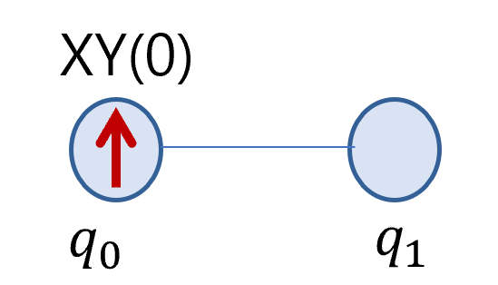
(a)

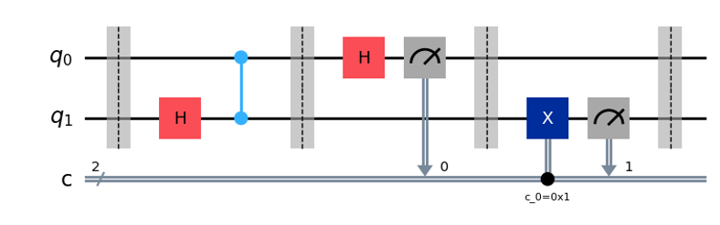
(b)

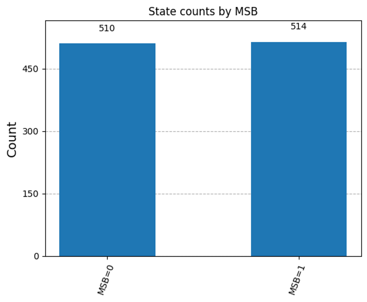
(c)

Figure 1: MBQC simulation based on Qiskit: $H$-gate. (a) The $H$-gate implementation in MBQC, where the qubit $q_{0}$ is the input and $q_{1}$ is the output; the arrow indicates the measurement angle in the $XY$ plane. (b) Test scenario: the input qubit $q_{0}$ is initialized in the $\ket{0}$ state. (c) After applying the $H$-gate, the state of $q_{1}$ collapses to either $\ket{0}$ or $\ket{1}$ with probability 0.5 upon measurement in the $Z$-basis.

III-D2 X Gate in MBQC

To implement the $X$-gate in MBQC, we require three qubits in a entangled state: an input qubit prepared in an arbitrary state $\ket{\psi}$ and two additional qubits prepared in the $\ket{+}$ state. By measuring the first qubit along the $X(0)$-axis and the second qubit along the $X(\pi)$-axis (i.e., the $X$-axis rotated by $\pi$ around the $Z$-axis), we can effectively apply an $X$-gate.

The process can be described as follows. After measuring the first qubit, the two-qubit system’s state becomes $\ket{s_{1}}_{1}\otimes X_{2}^{s_{1}}H_{2}\ket{\psi}_{2}$, where $s_{1}$ is the measurement outcome of the first qubit. Measuring the second qubit along the $X(\pi)$-axis results in the state $\ket{s_{1}}_{1}\otimes\ket{s_{2}}_{2}\otimes X_{3}^{s_{2}}H_{3}Z_{3}X_{3}^{s_{1}}H_{3}\ket{\psi}_{3}$. Using the equations $HZ=XH$, this state simplifies to $\ket{s_{1}}_{1}\otimes\ket{s_{2}}_{2}\otimes X_{3}^{s_{2}}X_{3}Z_{3}^{s_{1}}\ket{\psi}_{3}$. Further simplifying with the identity $XZ=(-1)ZX$, the state becomes $\ket{s_{1}}_{1}\otimes\ket{s_{2}}_{2}\otimes X_{3}^{s_{2}}Z_{3}^{s_{1}}(-1)X_{3}\ket{\psi}_{3}$. Thus, by applying corrections based on $s_{1}$ and $s_{2}$, we achieve the desired $X$-gate on the input qubit with a global phase factor of $(-1)$.

Fig. 2 shows a simple test using Qiskit to simulate this process. Fig. 2a represents the $X$-gate as implemented in MBQC, Fig. 2b shows the circuit used to simulate this $X$-gate, and Fig. 2c presents the results from 1024 executions of the circuit-based simulation.

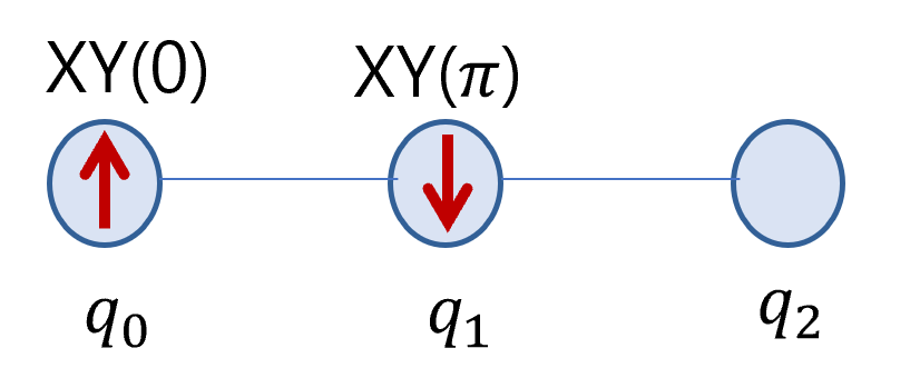
(a)

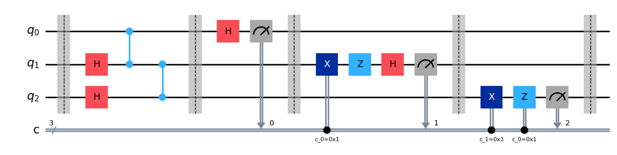
(b)

(c)

Figure 2: MBQC simulation based on Qiskit: $X$-gate. (a) The $X$-gate in MBQC, where the qubit $q_{0}$ is the input and $q_{2}$ is the output; the arrow indicates the measurement angle on the $XY$ plane. (b) Test scenario: the input qubit $q_{0}$ is initialized in the $\ket{0}$ state. (c) After applying the $X$-gate, the state of $q_{2}$ becomes $\ket{1}$ upon measurement in the $Z$-basis.

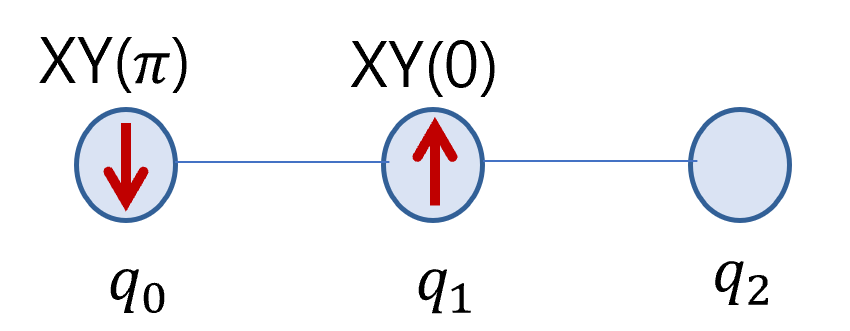
(a)

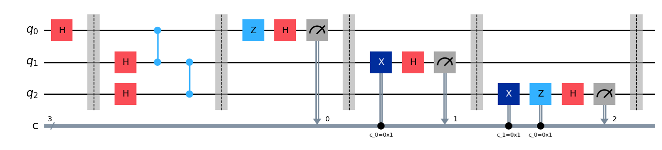
(b)

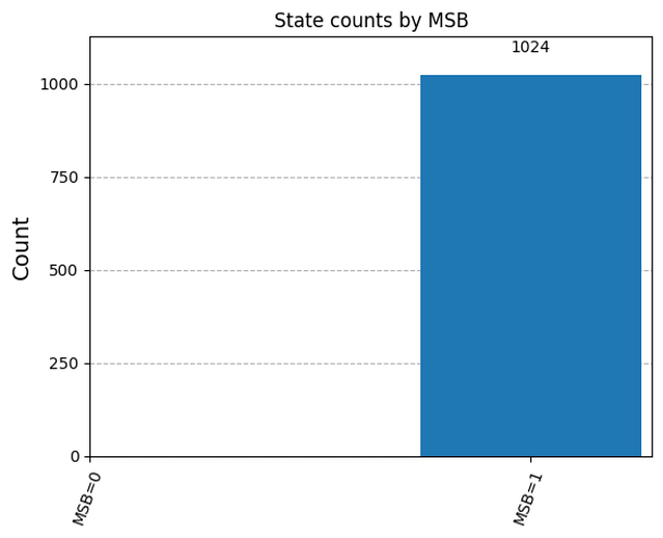
(c)

Figure 3: MBQC simulation using Qiskit: $Z$-gate. (a) The $Z$-gate in MBQC, where qubit $q_{0}$ is the input and $q_{2}$ is the output; the arrow indicates the measurement angle in the $XY$ plane. (b) Test scenario: the input qubit $q_{0}$ is initialized in the $\ket{+}$ state. (c) After applying the $Z$-gate, the state of $q_{2}$ becomes $\ket{-}$, then collapses to $\ket{1}$ upon measurement in the $X$-basis.

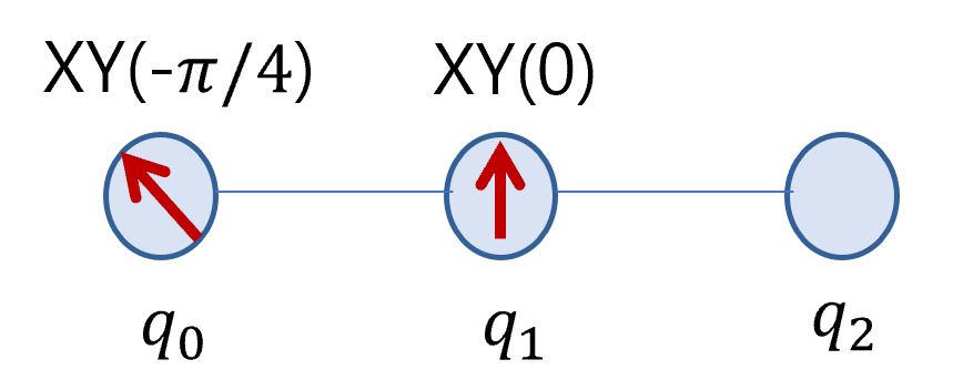
(a)

(b)

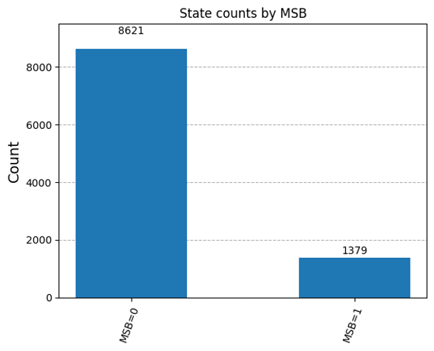
(c)

Figure 4: MBQC simulation using Qiskit: $T$-gate. (a) The $T$-gate in MBQC, where qubit $q_{0}$ is the input and $q_{2}$ is the output; the arrow indicates the measurement angle in the $XY$ plane. (b) Test scenario: the input qubit $q_{0}$ is initialized in the $\ket{+}$ state. (c) After applying the $T$-gate, the state of $q_{2}$ becomes $\ket{+_{\pi/4}}=\frac{1}{\sqrt{2}}(\ket{0}+e^{i\pi/4}\ket{1})$, which collapses to $\ket{0}$ with probability $\cos^{2}(\pi/8)\approx 0.8536$ upon $X$-basis measurement.

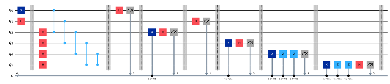
(a)

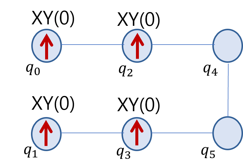
(b)

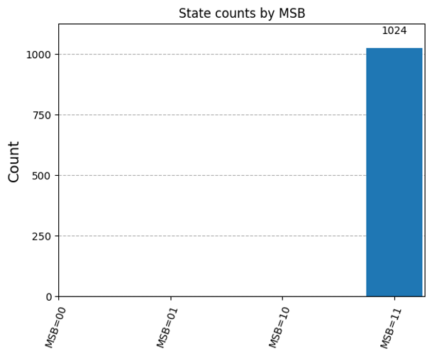
(c)

Figure 5: MBQC simulation using Qiskit: $CZ$-gate. (a) The $CZ$-gate in MBQC, where qubits $q_{0}$ and $q_{1}$ are the inputs, and $q_{4}$ and $q_{5}$ are the outputs; the arrow indicates the measurement angle in the $XY$ plane. (b) Test scenario: the input state is $q_{0},q_{1}=\ket{1}\otimes\ket{+}$. After applying the $CZ$-gate, (c) the output state becomes $\ket{1}\otimes\ket{-}$. Both qubits then collapse to $\ket{1}$ upon $Z$-basis measurement on $q_{4}$ and $X$-basis measurement on $q_{5}$.

III-D3 $R_{Z}(\theta)$-Gate in MBQC

To implement the $R_{Z}(\theta)$-gate in MBQC, we require three qubits in an entangled state: an input qubit initialized in an arbitrary state $\ket{\psi}$ and two additional qubits prepared in the $\ket{+}$ state. To apply the $R_{Z}(\theta)$-gate, we first measure the first qubit along the $X(-\theta)$-axis and then measure the second qubit along the $X(0)$-axis.

The process can be described as follows. After measuring the first qubit, the resulting state of the two-qubit system is $\ket{s_{1}}_{1}\otimes X_{2}^{s_{1}}H_{2}R_{Z}(\theta)_{2}\ket{\psi}_{2}$, where $s_{1}$ is the measurement outcome of the first qubit. Measuring the second qubit along the $X(0)$-axis yields the state $\ket{s_{1}}_{1}\otimes\ket{s_{2}}_{2}\otimes X_{3}^{s_{2}}H_{3}X_{3}^{s_{1}}H_{3}R_{Z}(\theta)_{3}\ket{\psi}_{3}$. Using the equation $HX=ZH$, this state simplifies to $\ket{s_{1}}_{1}\otimes\ket{s_{2}}_{2}\otimes X_{3}^{s_{2}}Z_{3}^{s_{1}}R_{Z}(\theta)_{3}\ket{\psi}_{3}$. By applying corrections based on $s_{1}$ and $s_{2}$, we obtain the desired result of an $R_{Z}(\theta)$-gate applied to the input qubit.

Figs. 3 and 4 show simple tests using Qiskit to simulate this process with $\theta=\pi$ for the $Z$-gate and $\theta=\pi/4$ for the $T$-gate, respectively.

III-D4 CZ Gate in MBQC

To implement the $CZ$-gate in MBQC, we require six qubits in an entangled state: two input qubits $\ket{\psi}$ and $\ket{\phi}$, along with four additional qubits prepared in the $\ket{+}$ state. The six qubits are arranged in a $2\times 3$ grid, with the first row containing qubits $q_{0}$ (input: $\ket{\psi}$), $q_{2}$, and $q_{4}$, and the second row containing qubits $q_{1}$ (input: $\ket{\phi}$), $q_{3}$, and $q_{5}$. When the qubits are entangled as shown in Fig. 5(b), the $CZ$-gate can be applied to the two input qubits by measuring $q_{0}$, $q_{1}$, $q_{2}$, and $q_{3}$ sequentially along the $X(0)$-axis.

This process can be described as follows. After measuring the first row, the resulting state is $\ket{s_{0}}_{0}\otimes\ket{s_{2}}_{2}\otimes X_{4}^{s_{2}}Z_{4}^{s_{0}}\ket{\psi}_{4}$. Similarly, after measuring the second row, the state is $\ket{s_{1}}_{1}\otimes\ket{s_{3}}_{3}\otimes X_{5}^{s_{3}}Z_{5}^{s_{1}}\ket{\phi}_{5}$. Considering the $CZ$-gate interaction between $q_{4}$ and $q_{5}$, the state can be written as:

$$CZ(X_{4}^{s_{2}}Z_{4}^{s_{0}}\ket{\psi}_{4}\otimes X_{5}^{s_{3}}Z_{5}^{s_{1}}\ket{\phi}_{5}).$$

Using the equations $CZ(X\otimes I)=(X\otimes Z)CZ$ and $CZ(I\otimes X)=(Z\otimes X)CZ$, this expression can be further simplified to:

$$(X_{4}^{s_{2}}Z_{4}^{s_{3}}\otimes X_{5}^{s_{3}}Z_{5}^{s_{2}})CZ(Z_{4}^{s_{0}}\ket{\psi}_{4}\otimes Z_{5}^{s_{1}}\ket{\phi}_{5}).$$

Applying the identities $CZ(Z\otimes I)=(Z\otimes I)CZ$ and $CZ(I\otimes Z)=(I\otimes Z)CZ$, we obtain:

$$(X_{4}^{s_{2}}Z_{4}^{s_{3}}Z_{4}^{s_{0}}\otimes X_{5}^{s_{3}}Z_{5}^{s_{2}}Z_{5}^{s_{1}})CZ(\ket{\psi}_{4}\otimes\ket{\phi}_{5}).$$

Using the measurement outcomes $s_{0}$, $s_{1}$, $s_{2}$, and $s_{3}$, we can apply the necessary corrections to achieve the desired $CZ$-gate on the two input qubits.

Fig. 5 shows a simple test using Qiskit to simulate this process. Fig. 5a represents the $CZ$-gate as implemented in MBQC, Fig. 5b shows the circuit used to simulate this $CZ$-gate, and Fig. 5c presents the results from 1024 executions of the circuit-based simulation.

IV Two-Qubit Grover’s Algorithm in MBQC using Qiskit

In this section, we implement and execute a two-qubit Grover’s algorithm using Qiskit to verify the correctness of the MBQC gates discussed in the previous sections.

IV-A Circuit-Based Two-Qubit Grover’s Algorithm

This section provides an explanation of the code-based implementation for the two-qubit Grover’s algorithm, which is the focus of our simulation. To implement this algorithm within a circuit-based framework, we require two logical qubits, as shown in Fig. 6. This implementation uses four gates: $H$, $X$, $Z$, and $CZ$, along with $Z$-axis measurements. The $CZ$-gate with surrounding $X$-gates serves to implement the oracle in Grover’s algorithm, shown here for the case where the oracle marks the state “00.” To implement an oracle for the “11” state, simply omit the $X$-gates around the $CZ$-gate for both qubits $q_{0}$ and $q_{1}$. For the “01” and “10” cases, apply the $X$-gate only to the qubit that does not match the oracle’s target state. Notably, the output qubits in the two-qubit Grover’s algorithm above are measured in the bitstring matching the oracle with a probability of 1.

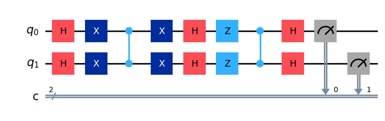
Figure 6: Circuit-based implementation of the two-qubit Grover’s algorithm.

IV-B Initial State Setup for MBQC Simulation

In this simulation, we use a total of 18 qubits to implement the two-qubit Grover’s algorithm within the MBQC framework. We arrange the qubits in a 2-row by 9-column grid, as shown in Fig. 7. Since Qiskit does not support two-dimensional indexing, we assign indices using the notation $q_{x,y}=q_{2y+x}$, where $x\in\{0,1\}$ and $y\in\{0,\dots,8\}$, for consistency.

For the initial MBQC setup, we prepare all qubits in the $\ket{+}$ state. Then, we apply the $CZ$-gate between all adjacent horizontal pairs and, as required by the algorithm (explained in the following subsection), between the vertical pairs $q_{4},q_{5}$ and $q_{14},q_{15}$. In this setup, we designate $q_{0}$ and $q_{1}$ as the input qubits and obtain the final computed outputs on $q_{16}$ and $q_{17}$. See Fig. 7 for reference.

IV-C Measurement Angle $\phi_{i}$

To perform the MBQC computation, we proceed with sequential measurements of the qubits in order from $q_{i}$ for $i\in\{0,\dots,15\}$. The measurement basis determines the MBQC algorithm, so in this section, we define the measurement basis angle $\phi_{i}$ for each qubit $q_{i}$.

Since the MBQC initial setting is in the $\ket{+}$ state, we omit the initial $H$-gates used in the circuit-based two-qubit Grover algorithm. To implement the $X$-gate on each input qubit $q_{0}$ and $q_{1}$, we use the qubit chains $q_{0}-q_{2}-q_{4}$ and $q_{1}-q_{3}-q_{5}$. The measurement procedure is as follows: measure $q_{0}$ and $q_{1}$ with $M^{0}_{i}$. If an $X$-gate is required for qubit $q_{0}$(or $q_{1}$) based on the oracle, measure $q_{2}$(or $q_{3}$) with $M^{\pi}_{i}$; otherwise, measure with $M^{0}_{i}$. To apply the $CZ$-gate, six qubits are needed. However, these qubits can overlap with those used for the $X$-gates, so we just initialize the $CZ$-gate on $q_{4}$ and $q_{5}$. For the next $X$-gate application after the $CZ$-gate, we use the chains $q_{4}-q_{6}-q_{8}$ and $q_{5}-q_{7}-q_{9}$. The measurement procedure is the same as for the first $X$-gate: measure $q_{4}$ and $q_{5}$ with $M^{0}_{i}$, and if the $X$-gate is required, measure $q_{6}$(or $q_{7}$) with $M^{\pi}_{i}$; otherwise, measure with $M^{0}_{i}$. Next, to apply the $H$-gate, we use qubits $q_{8}-q_{10}$ and $q_{9}-q_{11}$, measuring $q_{8}$ and $q_{9}$ with $M^{0}_{i}$. For the $Z$-gate followed by a $CZ$-gate, we use the chains $q_{10}-q_{12}-q_{14}$ and $q_{11}-q_{13}-q_{15}$, with $CZ$ initialized on $q_{14}$ and $q_{15}$. Measure $q_{10}$ and $q_{11}$ with $M^{\pi}_{i}$ and $q_{12}$ and $q_{13}$ with $M^{0}_{i}$. Finally, to apply the last $H$-gate, we use qubits $q_{14}-q_{16}$ and $q_{15}-q_{17}$. Measure $q_{14}$ and $q_{15}$ with $M^{0}_{i}$ to compute the final output qubits $q_{16}$ and $q_{17}$. The final output qubits are measured along the $Z$-axis to obtain the results after applying corrections.

To summarize, for a two-qubit Grover oracle set to “00,” the measurement angles without correction are $\phi_{i}=\pi$ for $i\in\{2,3,6,7,10,11\}$ and $\phi_{i}=0$ for the remaining indices. For an oracle set to “11,” neither of the input qubits requires an $X$-gate, so $\phi_{i}=\pi$ for $i\in\{10,11\}$ and $\phi_{i}=0$ for the remaining indices. See Fig. 7, which illustrates the two-qubit Grover’s algorithm in MBQC with the oracle set to “00.”

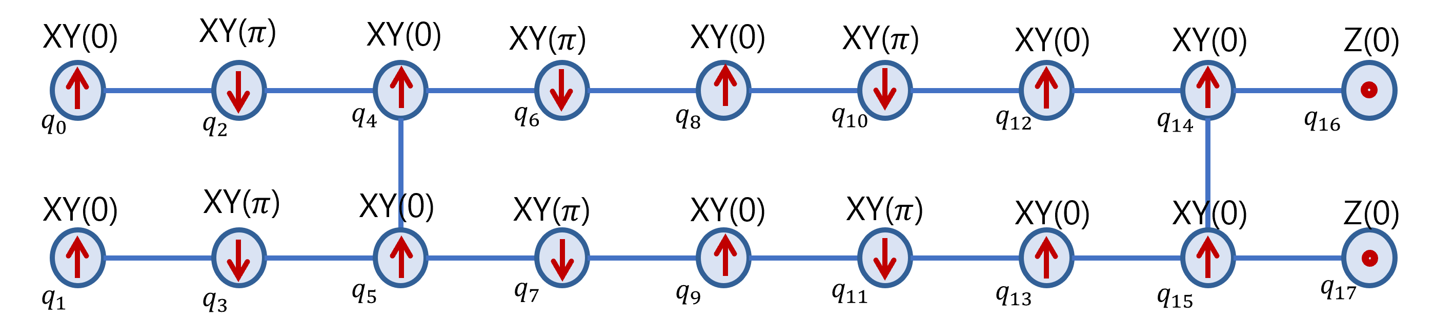
Figure 7: Two-Qubit Grover’s Algorithm in MBQC

IV-D Actual Measurement Angle $\phi_{i}^{\prime}$ with $X$ and $Z$ Corrections

The previously calculated angles $\phi_{i}$ for $i\in\{0,\dots,15\}$ do not include the necessary corrections for the measurement process. To obtain accurate MBQC computation results, we need to apply the actual measurement angles $\phi^{\prime}_{i}$, incorporating the corrections discussed in Section 3$B$.

In this simulation, we define the flow as follows: $I=\{0,1\}$, $O=\{16,17\}$, and $f(i)=i+2$. Thus, $S_{X}(i)=\{i-2\}$ for $i\in[2,17]$. For $S_{Z}$, the calculation method varies depending on the number of qubits connected to each qubit by $CZ$-gates. To account for all cases in this simulation, we define the set $VCZ$ as the indices of qubits connected by vertical $CZ$-gates, specifically where $i$ and $i+1$ (or $i$ and $i-1$) are linked by a $CZ$-gate. If $i\in VCZ$ and the qubit $i$ is even, then $S_{Z}(i)=\{i-4,i-1\}$. If $i$ is odd, then $S_{Z}(i)=\{i-4,i-3\}$. For qubits without vertical $CZ$-gate connections, $S_{Z}(i)=\{i-4\}$. Referring to Fig. 7, in this simulation, $VCZ=\{4,5,14,15\}$. Summarizing, we have:

$$S_{X}(i) =\emptyset, i\in[0,1]$$ (8)

$$S_{X}(i) =\{i-2\}, i\in[2,17]$$

$$S_{Z}(i) =\emptyset, i\in[0,3]$$

$$S_{Z}(i) =\{i-4\}, i\in[4,17]\setminus(VCZ=\{4,5,14,15\})$$

$$S_{Z}(i) =\{i-4,i-1\}, i\in\text{even}VCZ=\{4,14\}$$

$$S_{Z}(i) =\{i-4,i-3\}, i\in\text{odd}VCZ=\{5,15\}$$

By using (7) and (8), we can simulate the actual measurement angles $\phi^{\prime}_{i}$ for the two-qubit Grover’s algorithm in MBQC, including necessary corrections.

IV-E Implementation and Results

Algorithm 1 presents the initial setup for the MBQC two-qubit Grover’s algorithm. Referring to Fig. 7, we prepare all qubits in the $\ket{+}$ state, the initial setting for MBQC, by setting each qubit (representing a vertex) to $\ket{+}$. In Qiskit, qubits are initialized in the $\ket{0}$ state by default, so we apply an $H$-gate to prepare them in the $\ket{+}$ state. Next, we apply $CZ$-gates to establish the initial MBQC state by adding $CZ$ operations between all horizontally adjacent qubits, as well as between vertically adjacent qubits at indices specified by the $VCZ$ set.

Algorithm 1 MBQC Two-Qubit Grover Simulation: MBQC Initial State Setting

 Input: circuit, the number of qubits $n$, $VCZ$

 Output: circuit

 for $i$ in $[0,n-1]$ do

  circuit.h($i$)

 end for

 $j=n/2$

 for $i$ in $[0,j-2]$ do

  circuit.cz($2i,2i+2$)

  circuit.cz($2i+1,2i+3$)

 end for

 for $i$ in $VCZ$ do

  if $i\mod 2=0$ then

   circuit.cz($i,i+1$)

  end if

 end for

 return  circuit

Algorithm 2 presents the simulation of $M^{\phi^{\prime}}$ (referring to (7)) using Qiskit. Conditional gate applications based on prior measurement outcomes are implemented with Qiskit’s circuit.gate($i$).c_if($j,1$) function, which applies a gate to qubit $i$ if the measurement outcome of qubit $j$ is 1. We perform $Z$ and $X$ corrections using this function, apply gates corresponding to $M^{\phi}$, and finally use a $Z$-measurement to simulate $M^{\phi^{\prime}}$ on a circuit-based platform.

Algorithm 2 MBQC Two-Qubit Grover Simulation: Measurement with correction, $M^{\phi^{\prime}}$

 Input: circuit, qubit index $i$, initial angle $\phi$, $VCZ$

 Output: circuit {Z-correction}

 if $i-4\geq 0$ then

  circuit.z($i$).c_if($i-4,1$)

 end if

 if $i\in VCZ$ and $i\mod 2=0$ and $i-1\geq 0$ then

  circuit.z($i$).c_if($i-1,1$)

 end if

 if $i\in VCZ$ and $i\mod 2=1$ and $i-3\geq 0$ then

  circuit.z($i$).c_if($i-3,1$)

 end if{X-correction}

 if $i-2\geq 0$ then

  circuit.x($i$).c_if($i-2,1$)

 end if{$M_{i}^{\phi_{i}}$ measurement}

 circuit.rz($-\phi,i$)

 circuit.h($i$)

 circuit.measure($i,i$)

 return  circuit

Algorithm 3 presents the main MBQC simulation of the two-qubit Grover’s algorithm using Qiskit. By employing Algorithms 1 and 2, we implemented the entire two-qubit Grover’s algorithm.

First, we set up the MBQC initial state with $n=18$ qubits and a vertical $CZ$-gate index set $VCZ=\{4,5,14,15\}$, as required by the algorithm. Then, based on the MBQC layout and the two-bit oracle value for Grover’s algorithm, we assign the measurement angles $\phi_{i}$. And we perform measurements $M_{i}^{\phi^{\prime}}$ sequentially on all qubits except for the output qubits, in ascending index order. Finally, we apply $X$-corrections on the two output qubits to determine the result of the MBQC-based two-qubit Grover’s algorithm. Note that Grover’s algorithm verifies the computed result with a final $Z$-measurement, so $Z$-corrections on the output qubits are omitted as they do not influence the final outcome. However, if $Z$-corrections were significant for the output qubits, they should be included.

The result of Algorithm 3 (for oracle: “00”) is shown in Fig. 8, which illustrates the circuit used to simulate the MBQC two-qubit Grover’s algorithm. We performed quantum circuit simulation on a classical computing simulator provided by Qiskit. Fig. 9 displays the results of this simulation for each oracle value in Grover’s algorithm. For each oracle case of the two-qubit Grover’s algorithm (“00”, “01”, “10”, “11”), we verified the algorithm’s accuracy by executing 1024 shots for each circuit, confirming correct results in all cases.

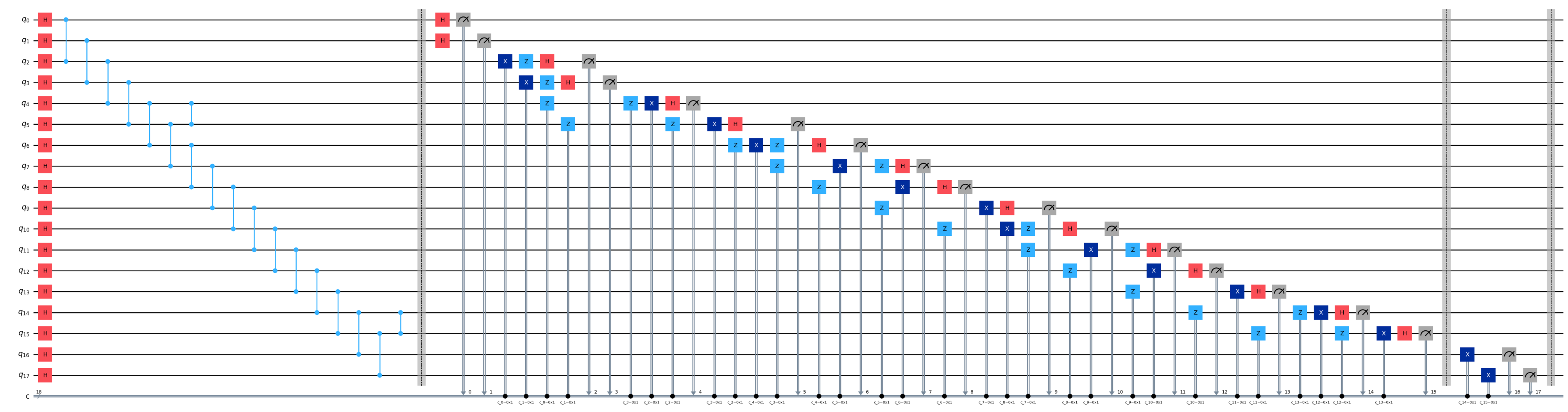
Figure 8: Circuit-Based Simulation of MBQC Two-Qubit Grover’s Algorithm

Algorithm 3 MBQC Two-Qubit Grover Simulation

 Input: the number of qubits $n=18$, $VCZ=\{4,5,14,15\}$, oracle

 Output: circuit {initial setting}

 circuit = Initialize_quantum_circuit(n,n)

 MBQC_Initial_State_Set(circuit,$n,VCZ$)          (Alg. 1) {set $\{\phi_{i}\}$}

 $\phi_{i}=0$ for $i\in[0,n-1]\setminus[10,11]$

 $\phi_{i}=\pi$ for $[10,11]$

 if oracle = “00” or “10” then

  $\phi_{i}=\pi$ for $i\in\{2,6\}$

 end if

 if oracle = “00” or “01” then

  $\phi_{i}=\pi$ for $i\in\{3,7\}$

 end if{inputs and intermediate qubits measurement}

 for $i$ in $[0,n-3]$ do

  $M^{\phi^{\prime}}(circuit,i,\phi_{i},VCZ)$                          (Alg. 2)

 end for{output qubits measurement with corrction}

 for $i$ in $[n-2,n-1]$ do

  if $i-2\geq 0$ then

   circuit.x($i$).c_if($i-2,1$)

  end if

  circuit.measure($i,i$)

 end for

 return  circuit

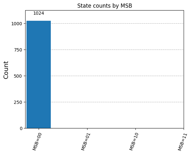
(a)

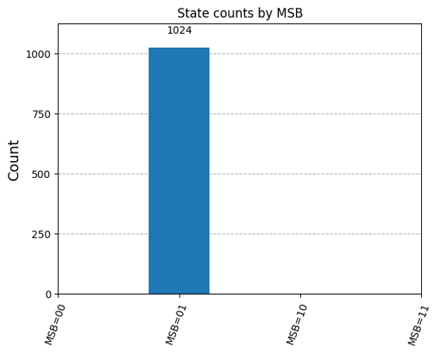
(b)

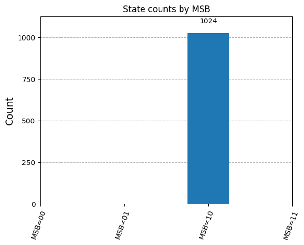
(c)

(d)

Figure 9: Results of circuit simulation when (a) Oracle: 00, (b) Oracle: 01, (c) Oracle: 10, (d) Oracle: 11

V UBQC Protocol on MBQC Two-Qubit Grover Simulation

In this section, we discuss the application of UBQC protocol to the MBQC-based two-qubit Grover’s algorithm, as implemented in the previous section, and present the results of our experiment.

V-A UBQC Protocol

The UBQC[7], is a quantum secure computation protocol between a quantum computing server, Bob, and a client, Alice. It allows Alice to delegate a desired quantum computation to Bob while preserving the privacy of her data and the computation details.

The protocol requires that Alice, as the client, can generate random quantum states in the set $\{\Ket{+_{\theta}}\,|\,\theta=0,\frac{\pi}{4},\dots,\frac{7\pi}{4}\}$, where $\Ket{+_{\theta}}=\frac{1}{\sqrt{2}}(\Ket{0}+e^{i\theta}\Ket{1})$, and send them to the server. The protocol operates as follows: Alice prepares the quantum computation she wants to delegate using an MBQC-based brickwork state, $\mathcal{G}_{n,m}$. Each qubit $\Ket{\psi_{x,y}}\in\mathcal{G}_{n,m}$ has a measurement angle $\phi_{x,y}$ determined by Alice, along with $X$-dependencies $D_{x,y}$ and $Z$-dependencies $D^{\prime}_{x,y}$ for error correction. Let $X_{x,y}$ and $Z_{x,y}$ denote these dependency sets. As the MBQC computation proceeds, the actual measurement angle $\phi^{\prime}_{x,y}$, incorporating error corrections, is calculated as follows. Let $s^{X}_{x,y}=\oplus_{i\in D_{x,y}}s_{i}$ be the parity of all measurement outcomes for qubits in $X_{x,y}$, and $s^{Z}_{x,y}=\oplus_{i\in D^{\prime}_{x,y}}s_{i}$ the parity of all outcomes for qubits in $Z_{x,y}$. Then the corrected angle is $\phi^{\prime}_{x,y}=(-1)^{s^{X}_{x,y}}\phi_{x,y}+s^{Z}_{x,y}\pi$.

Protocol 1 Universal Blind Quantum Computation[7]

1. Alice’s Preparation

For each column $x=1,\dots,n$:

For each row $y=1,\dots,m$:

Alice prepares $\Ket{\psi_{x,y}}\in_{R}\{\Ket{+_{\theta}}\,|\,\theta=0,\frac{\pi}{4},\dots,\frac{7\pi}{4}\}$,

and sends the qubits to Bob.

2. Bob’s Preparation

Bob entangles all received qubits according to their indices by applying $CZ$ gates between them to create the brickwork state $\mathcal{G}_{n\times m}$.

3. Interaction and Measurement

For each column $x=1,\dots,n$:

For each row $y=1,\dots,m$:

3.1 Alice computes $\phi^{\prime}_{x,y}$ with $s_{0,y}^{X}=s_{0,y}^{Z}=0$.

3.2 Alice selects $r_{x,y}\in_{R}\{0,1\}$ and

computes $\delta_{x,y}=\phi^{\prime}_{x,y}+\theta_{x,y}+\pi r_{x,y}$.

3.3 Alice transmits $\delta_{x,y}$ to Bob.

Bob measures in the basis $\{\Ket{+_{\delta_{x,y}}},\Ket{-_{\delta_{x,y}}}\}$. 3.4 Bob sends the result $s_{x,y}\in\{0,1\}$ to Alice.

3.5 If $r_{x,y}=1$, Alice flips $s_{x,y}$;

otherwise, she does nothing.

The UBQC protocol comprises three main phases, detailed in Protocol 1. These steps ensure that Bob cannot access the actual computational details or its outcome, as Alice’s randomization obscures the true measurement basis at every step.

V-B Two-Qubit Grover with UBQC Protocol

In this simulation, we apply the UBQC protocol to the MBQC-based two-qubit Grover’s algorithm. Since our objective is to validate the quantum computation itself, we omit the actual quantum states and classical bit transmission between Alice and Bob. Although using a brickwork state could obscure the shape of the MBQC circuit, this experiment assumes that the server (Bob) is aware of the shape of MBQC but does not know measurement angles $\phi_{i}$, which is essential for concealing the oracle information in MBQC Grover’s algorithm. Specifically, in this case, the protocol aims to hide the measurement angles for qubits $q_{2},q_{3},q_{6},q_{7}$, which contain the oracle information. Consequently, unlike the UBQC protocol’s use of a brickwork state, we apply the protocol directly to the $2\times 9$ qubit configuration introduced in the previous chapter.

To implement this protocol within the simulation discussed in Section 4, some modifications are required:

• First, unlike the initial setup where all qubits were in the $\Ket{+}$ state, Alice’s preparation is now adjusted according to her random key.

• Second, instead of simulating measurements with only $\phi^{\prime}$ values from Protocol 1 in Section 4, this protocol requires measurements based on $\delta_{x,y}=\phi^{\prime}+\theta_{x,y}+\pi r_{x,y}$.

Apart from these two changes, other steps involve classical computation processing. We will focus on explaining these two points.

V-B1 Alice’s Preparation in Qiskit

To prepare states in $\{\Ket{+_{\theta}}\,|\,\theta=0,\frac{\pi}{4},\dots,\frac{7\pi}{4}\}$ in Qiskit, we can rotate the $\Ket{+}$ state around the $Z$-axis by angles $0,\frac{\pi}{4},\dots,\frac{7\pi}{4}$. This can be achieved by using Qiskit’s rotation gates or by combining the $Z=R_{Z}(\pi)$ and $T=R_{Z}(\pi/4)$ gates. For this simulation, instead of Alice sending these states to the server, we generate them directly on the server as mentioned before.

V-B2 Measurement Method for UBQC, $M^{\delta}$

To simulate measurements in the basis $\{\Ket{+_{\delta_{x,y}}},\Ket{-_{\delta_{x,y}}}\}$ where $\delta_{x,y}=\phi^{\prime}_{x,y}+\theta_{x,y}+\pi r_{x,y}$ and $\theta_{x,y}\in\{0,\frac{\pi}{4},\dots,\frac{7\pi}{4}\}$ in Qiskit, we use the property that $M_{i}^{\phi+\theta}=M_{i}^{\phi}R_{Z}(-\theta)$ for any $\theta$. Thus, the measurement can be expressed as follows:

$$M_{x,y}^{\delta_{x,y}}=M_{x,y}^{\phi^{\prime}_{x,y}}R_{Z}(-\theta_{x,y})R_{Z}(\pi r_{x,y})$$ (9)

To simulate $M_{x,y}^{\delta_{x,y}}$ in Qiskit, we apply the gates $R_{Z}(-\theta_{x,y})R_{Z}(\pi r_{x,y})$ before performing the measurement $M_{x,y}^{\phi^{\prime}_{x,y}}$ as described in Section 4.

V-C Implementation and Results

Algorithm 4 shows the initial setup for the privacy-preserving version of the MBQC two-qubit Grover’s algorithm. Unlike Algorithm 1, where each state is set to $\ket{+}$, here we initialize each qubit in a random state $\ket{+_{\theta}}$, where $\theta\in_{R}\{0,\pi/4,\dots,7\pi/4\}$. Thus, we initialize each qubit in the $\ket{+}$ state and apply a random rotation $R_{Z}(\theta_{i})$ for a randomly chosen $\theta_{i}$ from the set $\{0,\pi/4,\dots,7\pi/4\}$ to each qubit $q_{i}$, resulting in the $\ket{+_{\theta_{i}}}$ state. The rest of the process remains the same as in Algorithm 1.

Algorithm 4 Blind MBQC Two-Qubit Grover Simulation:
Blind Initial State Setting

 Input: circuit, $n$, $\{\theta_{i}\}_{i\in[0,n-1]}$, $VCZ$

 Output: circuit

 for $i$ in $[0,n-1]$ do

  circuit.h($i$)

  circuit.rz($\theta_{i},i$)

 end for

 $j=n/2$

 for $i$ in $[0,j-2]$ do

  circuit.cz($2i,2i+2$)

  circuit.cz($2i+1,2i+3$)

 end for

 for $i$ in $VCZ$ do

  if $i\mod 2=0$ then

   circuit.cz($i,i+1$)

  end if

 end for

 return  circuit

Algorithm 5 presents how to simulate $M^{\delta}$ (as defined in (9)) using Qiskit. Depending on the random value $r_{i}\in_{R}\{0,1\}$, apply a $Z$-gate if $r_{i}=1$; otherwise, do nothing. Then, apply a rotation about the $Z$-axis by $-\theta$ on qubit $i$. By using Algorithm 2, complete the measurement for $M^{\delta}$.

Algorithm 5 Blind MBQC Two-Qubit Grover Simulation:
Blind Measurement with correction $M^{\delta}$

 Input: circuit, qubit index $i$, $\theta_{i}$, $r_{i}$, $\phi_{i}$, $VCZ$

 Output: circuit {$\pi r_{i}$-Rotation}

 if $r_{i}=1$ then

  circuit.z($i$)

 end if{$(-\theta_{i})$-Rotation}

 circuit.rz($-\theta_{i},i$) {$M_{i}^{\phi^{\prime}}$ measurement}

 $M^{\phi^{\prime}}(circuit,i,\phi_{i},VCZ)$                         (Alg. 2)

 return  circuit

Algorithm 6 presents the main simulation of the blind two-qubit Grover’s algorithm using Qiskit. We implemented the complete blind two-qubit Grover’s algorithm using Algorithms 4 and 5.

First, we set the number of qubits to $n=18$, specify the indices of qubits connected by vertical $CZ$-gates as $VCZ=\{4,5,14,15\}$, and use the MBQC measurement angles $\{\phi_{i}\}$ as in Algorithm 3. We then generate random arrays $\{\theta_{i}\}$ and $\{r_{i}\}$ for the blind protocol and use Algorithm 4 for the initial setup. Subsequently, we conduct measurements $M_{i}^{\delta}$ on all qubits in ascending index order, excluding the output qubits.

In the blind protocol, if $r_{i}=1$, we need to flip the measurement outcome $s_{i}$. However, since Qiskit does not allow direct modification of the classical register storing the measurement result, we implement the flip process by applying an $X$-gate to the qubit $q_{i}$ after its measurement, followed by a second measurement. The final measurement of the output qubits follows the same procedure as in Algorithm 3.

The result of Algorithm 6 (with the oracle set to “00”) is shown in Fig. 10, which shows the circuit used to simulate the blind MBQC two-qubit Grover’s algorithm.

In the blind two-qubit Grover’s algorithm simulation, Bob cannot obtain information about the output qubits due to the masking of $s_{14}$ and $s_{15}$ by the random values $r_{14}$ and $r_{15}$. Similarly, Bob cannot infer any information about the oracle, as the $\phi_{i}$ values are masked by the hidden angles $\theta_{i}$.

To demonstrate the confidentiality of the blind protocol, we conducted two simulations for comparison by adding simple exception handling: one from Bob’s perspective, where the $s_{14}$ and $s_{15}$ flips were not performed, and one from Alice’s perspective (Algorithm 6), where each $s_{i}$ was flipped based on Alice’s random values $r_{i}$.

In Bob’s view, where the $s_{14}$ and $s_{15}$ flips were omitted, we observed a uniformly distributed measurement outcome, as shown in Fig. 11. Conversely, in Alice’s view, where the $s_{14}$ and $s_{15}$ flips were applied, the results were correct and matched those in Fig. 9. This simulation experimentally confirms the correctness of the blind protocol in the quantum circuit simulation.

Algorithm 6 Blind MBQC Two-Qubit Grover Simulation

 Input: the number of qubits $n=18$, $VCZ=\{4,5,14,15\}$, oracle

 Output: circuit {generate random array}

 $\theta_{i}\in_{R}\{0,\pi/4...,7\pi/4\}$ for $i\in[0,n-1]$

 $r_{i}\in_{R}\{0,1\}$ for $i\in[0,n-1]$ {initial setting}

 circuit = Initialize_quantum_circuit(n,n)

 Blind_Initial_State_Set(circuit,$n,\{\theta_{i}\},VCZ$)      (Alg. 4) {set $\{\phi_{i}\}$}

 $\phi_{i}=0$ for $i\in[0,n-1]\setminus[10,11]$

 $\phi_{i}=\pi$ for $[10,11]$

 if oracle = “00” or “10” then

  $\phi_{i}=\pi$ for $i\in\{2,6\}$

 end if

 if oracle = “00” or “01” then

  $\phi_{i}=\pi$ for $i\in\{3,7\}$

 end if{inputs and intermediate qubits measurement}

 for $i$ in $[0,n-3]$ do

  $M^{\delta}(circuit,i,\theta_{i},r_{i},\phi_{i},VCZ)$                     (Alg. 5)

  if $r_{i}=1$ then

   circuit.x($i$)

   circuit.measure($i,i$)

  end if

 end for{output qubits measurement with corrction}

 for $i$ in $[n-2,n-1]$ do

  if $i-2\geq 0$ then

   circuit.x($i$).c_if($i-2,1$)

  end if

  circuit.measure($i,i$)

 end for

 return  circuit

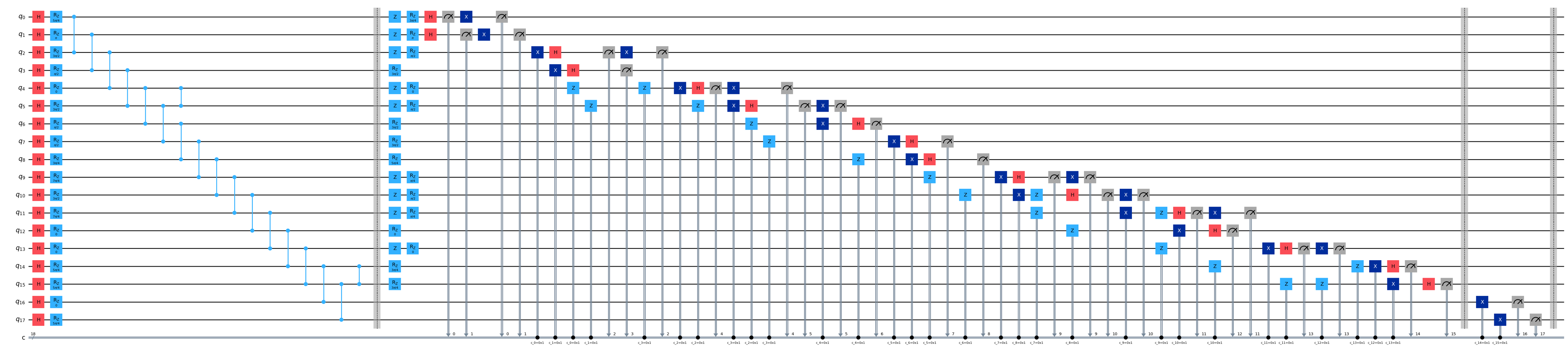
Figure 10: Circuit-Based Simulation of Blind MBQC Two-Qubit Grover’s Algorithm

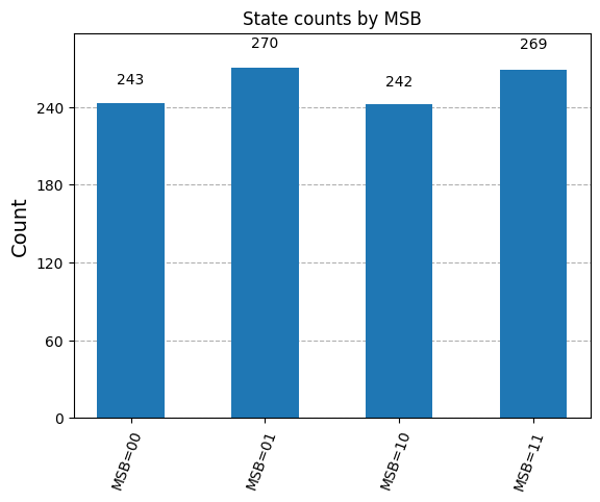
(a)

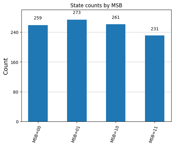
(b)

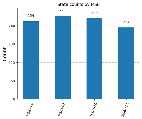
(c)

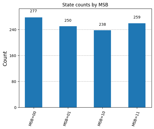
(d)

Figure 11: Results of circuit simulation with Bob’s view when (a) Oracle: 00, (b) Oracle: 01, (c) Oracle: 10, (d) Oracle: 11

VI Conclusion

This study successfully demonstrates a method for simulating MBQC on circuit-based quantum platforms, with specific emphasis on privacy-preserving protocols. Leveraging the two-qubit Grover’s algorithm as a test case, we validated our MBQC simulation approach and further demonstrated its capability to maintain function privacy by integrating the UBQC protocol proposed by Broadbent et al [7]. This work presents the first complete simulation of the two-qubit Grover’s algorithm based on MBQC, with the implementation of UBQC for secure quantum computation.

The results highlight that MBQC, although theoretically equivalent to circuit-based quantum computation, requires specific considerations for efficient simulation on available quantum computing platform. By carefully managing the transformation of MBQC algorithm to circuit-based representations, our approach enables current quantum cloud platforms to support secure, privacy-preserving computations without excessive qubit overhead or unmanageable complexity. This capability could be instrumental in advancing practical quantum cloud computing by allowing clients to delegate computations securely and confidently.

Future research will focus on expanding this simulation framework to support more complex algorithms, improving efficiency, and minimizing resource requirements. Additionally, there is significant potential for further refinement of the privacy-preserving mechanisms within MBQC to meet the security demands of larger-scale quantum cloud services. This work lays foundational groundwork, bridging theoretical protocols and practical quantum computations, and presents an effective pathway for realizing secure quantum computing in cloud environments.

References

- [1] 2017.
- [2] Stefanie Barz, Elham Kashefi, Anne Broadbent, Joseph F. Fitzsimons, Anton Zeilinger, and Philip Walther. Demonstration of blind quantum computing. Science, 335(6066):303–308, 2012.
- [3] Stefanie Barz, Elham Kashefi, Anne Broadbent, Joseph F. Fitzsimons, Anton Zeilinger, and Philip Walther. Experimental verification of quantum computation. Nature Physics, 9:727–731, 2013.
- [4] Charles H. Bennett, Ethan Bernstein, Gilles Brassard, and Umesh Vazirani. Strengths and weaknesses of quantum computing. SIAM Journal on Computing, 26(5):1510–1523, 1997.
- [5] Michel Boyer, Gilles Brassard, Peter Høyer, and Alain Tapp. Tight bounds on quantum searching. Fortschritte der Physik, 46(4–5):493–505, June 1998.
- [6] H. J. Briegel, D. E. Browne, W. Dür, R. Raussendorf, and M. Van den Nest. Measurement-based quantum computation. Nature Physics, 5(1):19–26, 2009.
- [7] Anne Broadbent, Joseph Fitzsimons, and Elham Kashefi. Universal blind quantum computation. In 2009 50th Annual IEEE Symposium on Foundations of Computer Science, pages 517–526, 2009.
- [8] Dan E. Browne and Hans J. Briegel. One-way quantum computation: A tutorial introduction. arXiv preprint quant-ph/0603226, 2006.
- [9] Daniel E. Browne and Terry Rudolph. Resource-efficient linear optical quantum computation. Phys. Rev. Lett., 95:010501, Jun 2005.
- [10] Andrew M. Childs. Secure assisted quantum computation. Quantum Info. Comput., 5(6):456–466, September 2005.
- [11] Vincent Danos and Elham Kashefi. Determinism in the one-way model. Phys. Rev. A, 74:052310, Nov 2006.
- [12] Vincent Danos, Elham Kashefi, and Prakash Panangaden. Parsimonious and robust realizations of unitary maps in the one-way model. Phys. Rev. A, 72:064301, Dec 2005.
- [13] Vedran Dunjko, Joseph F. Fitzsimons, Christopher Portmann, and Renato Renner. Composable security of delegated quantum computation. In Palash Sarkar and Tetsu Iwata, editors, Advances in Cryptology – ASIACRYPT 2014, pages 406–425, Berlin, Heidelberg, 2014. Springer Berlin Heidelberg.
- [14] Vedran Dunjko, Elham Kashefi, and Anthony Leverrier. Blind quantum computing with weak coherent pulses. Phys. Rev. Lett., 108:200502, May 2012.
- [15] Joseph F. Fitzsimons and Elham Kashefi. Unconditionally verifiable blind quantum computation. Phys. Rev. A, 96:012303, Jul 2017.
- [16] Lov K. Grover. A fast quantum mechanical algorithm for database search. In Proceedings of the Twenty-Eighth Annual ACM Symposium on Theory of Computing, STOC ’96, page 212–219, New York, NY, USA, 1996. Association for Computing Machinery.
- [17] Ali Javadi-Abhari, Matthew Treinish, Kevin Krsulich, Christopher J. Wood, Jake Lishman, Julien Gacon, Simon Martiel, Paul D. Nation, Lev S. Bishop, Andrew W. Cross, Blake R. Johnson, and Jay M. Gambetta. Quantum computing with qiskit, 2024.
- [18] Richard Jozsa. An introduction to measurement based quantum computation, 2005.
- [19] Elham Kashefi and Anna Pappa. Multiparty delegated quantum computing. Cryptography, 1(2):12, July 2017.
- [20] Muhammad Kashif and Saif Al-Kuwari. Qiskit as a simulation platform for measurement-based quantum computation. In 2022 IEEE 19th International Conference on Software Architecture Companion (ICSA-C), pages 152–159, 2022.
- [21] David C. McKay, Thomas Alexander, Luciano Bello, Michael J. Biercuk, Lev Bishop, Jiayin Chen, Jerry M. Chow, Antonio D. Córcoles, Daniel Egger, Stefan Filipp, Juan Gomez, Michael Hush, Ali Javadi-Abhari, Diego Moreda, Paul Nation, Brent Paulovicks, Erick Winston, Christopher J. Wood, James Wootton, and Jay M. Gambetta. Qiskit backend specifications for openqasm and openpulse experiments, 2018.
- [22] Tomoyuki Morimae and Keisuke Fujii. Blind quantum computation protocol in which alice only makes measurements. Phys. Rev. A, 87:050301, May 2013.
- [23] Michael A. Nielsen and Isaac L. Chuang. Quantum Computation and Quantum Information. Cambridge University Press, 2010.
- [24] Qiskit Development Team. Qiskit: An open-source quantum computing software development framework, 2023.
- [25] Robert Raussendorf and Hans J. Briegel. A one-way quantum computer. Phys. Rev. Lett., 86:5188–5191, May 2001.
- [26] Robert Raussendorf, Daniel E. Browne, and Hans J. Briegel. Measurement-based quantum computation on cluster states. Phys. Rev. A, 68:022312, Aug 2003.
- [27] Peter W. Shor. Polynomial-time algorithms for prime factorization and discrete logarithms on a quantum computer. SIAM Journal on Computing, 26(5):1484–1509, 1997.
- [28] Yuki Takeuchi and Tomoyuki Morimae. Verification of many-qubit states. Phys. Rev. X, 8:021060, Jun 2018.
- [29] various authors. Qiskit Textbook. Github, 2023.
- [30] Petros Wallden. Introduction to quantum computing. University Lectures, 2018.
- [31] Ieva Čepaitė. Simulation of networked quantum computing on encrypted data, 2022.