Network Calculus-based Deadline-Adaptive
Online Admission Control for ET Traffic in TSN

Abstract

Time-Sensitive Networking (TSN) has been a promising standard for deterministic communication in Internet of Things (IoT) applications. Recent developments have necessitated dynamic reconfigurations during system operations. Current research on admission control in TSN mainly focuses on time-triggered (TT) traffic, but the more flexible event-triggered (ET) traffic with latency guarantee requirements also needs attention. The challenge in the admission control method for time-critical ET traffic is to quickly admit incremental flow while ensuring deadline guarantees for both incremental and existing flows. However, conventional configuration methods, which require ex-post schedulability feedback verification during solution space searches to ensure real-time requirements, are inappropriate for online admission control due to their high time consumption. Therefore, we propose a fast and high-utilization deadline-adaptive online admission control method for ET traffic based on a network calculus approach, leveraging the TSN/ATS+CBS (asynchronous traffic shaper and credit-based shaper) architecture and a novel prior performance analysis model. This method benefits from ATS in reducing the impact on existing flows and avoids the need for ex-post verification during the iterative optimization process used by conventional methods. Moreover, it adaptively balances residual resources with deadline awareness during the admission process to enhance network resource utilization. Evaluations on synthetic test cases demonstrate that, compared to the state-of-the-art, our method achieves an average 59% increase in admitted flows and an average 95% reduction in admission time. Additionally, evaluations on realistic test cases reveal that our method postpones the occurrence of bottleneck egress ports and first rejection during the admission process, thereby enhancing adaptability.

I Introduction

The integration of Internet of Things (IoT) technology into the automotive, aerospace, and industrial automation domains has accelerated advancements in intelligence and connectivity across these sectors. As IoT applications in these domains increasingly require high determinism and dynamic adaptability, the demand for deterministic communication networks that enable flexible reconfiguration has grown significantly. Time-Sensitive Networking (TSN), which supports deterministic communication, integrates the Centralized Network Configuration (CNC) element and the Centralized User Configuration (CUC) element through IEEE 802.1 Qcc[1] to enable dynamic configuration. However, while 802.1 Qcc standardizes interfaces and protocols, the specific configuration methods remain an area with numerous open questions. The challenge of reconfiguration for real-time networks is to enhance online admission utility, such as maximizing the number of admitted flows and resource utilization, while ensuring the real-time requirements of both incremental and existing flows and reducing the reconfiguration time.

For time-triggered (TT) traffic implemented by scheduling mechanisms such as time-aware shaper (TAS) [2] and cyclic queuing forwarding (CQF) [3], configuration involves designing scheduling tables, with schedulability ensured by incorporating deadline constraints into the scheduling table design. In order to reduce the computational complexity of static configuration methods, several online admission control methods for TT traffic have been developed for dynamic scenarios [4, 5, 6, 7, 8, 9, 10], enabling the addition and removal of traffic. For event-triggered (ET) traffic implemented by scheduling mechanisms such as strict priority (SP) [11], credit-based shaper (CBS) [12], and asynchronous traffic shaper (ATS) [13], the configuration just involves setting critical parameters. This offers more flexibility than designing scheduling tables for TT traffic, making ET traffic essential to supporting real-time communications. Nevertheless, unlike TT traffic, ET traffic requires dedicated performance analysis [14, 15, 16] to ensure deadline guarantees, serving as feedback verification during configuration optimization. The study [17] has shown that performance analysis takes up more than 90% of the total configuration time, which may be unacceptable in dynamic reconfiguration scenarios. Although recent incremental performance analysis [18] for small configuration changes eliminates the need for global analysis with every configuration iteration and greatly reduces evaluation complexity, it still cannot eliminate the need for feedback verification. When there are massive flows varying simultaneously, the complexity of incremental analysis may approach that of global performance analysis of the network. Guck et al.[19] and Maile et al.[20] have provided admission control methods for networks using SP and CBS, respectively. They ensure real-time requirements by setting delay budgets on queues and implementing delay-constrained least-cost (DCLC) routing across the network at runtime. However, this online DCLC routing increases admission time, and the fixed, unchangeable delay budgets established to handle burst cascades reduce the adaptability to dynamic flows, thereby impacting admission capacity. To address these issues, we propose a fast and high-utilization deadline-adaptive online admission control method based on a novel prior performance analysis model [21], leveraging the TSN/ATS+CBS architecture. Our main contributions are summarized as follows:

• We develop an online admission control framework that, assisted by ATS to reduce the reconfiguration domain, achieves dynamic minimum bandwidth allocation and reclamation with prior performance guarantees. This approach avoids iterative optimization with feedback verification and online routing, thereby providing a faster solution.

• We propose a deadline-adaptive adjustment strategy based on network-calculus (NC) theory to guarantee real-time requirements. This strategy dynamically balances residual resources with deadline awareness during the online admission control process, thus improving network resource utilization.

• We evaluate our method compared to the state-of-the-art in various large-scale cases. The results from synthetic test cases show that our method increases the number of admitted flows by an average of 59% and reduces the admission time by an average of 95%. Evaluations across three realistic test cases demonstrate that our method postpones the occurrence of bottleneck egress ports and the first rejection during the admission process, thereby improving adaptability.

The rest of this article is organized as follows. Section II provides the background of the study. Section III introduces the online admission control framework, and Section 4 proposes the deadline-adaptive local deadline adjustment strategy. Experimental evaluations are conducted in Section V. Finally, Section VI concludes.

Figure 1: (a) a TSN network example, (b) TSN/ATS+CBS egress port architecture.

II Background

II-A TSN/ATS+CBS Network and Flow Model

In a TSN network, the network graph $\mathcal{G}=(\mathcal{N},\mathcal{L})$ consists of a set of nodes $\mathcal{N}$, including end-systems (ESs) and switches (SWs), and a set of physical links $\mathcal{L}$, as shown in Fig. 1(a). We define $(u,v)\in\mathcal{L}$ as the physical link from node $u$ to node $v$, also representing the corresponding egress port, with a transmission rate of $C$. For each egress port, this paper considers a hybrid architecture of ATS [13, 22] and CBS[12], referred to as TSN/ATS+CBS [23], as shown in Fig. 1(b). This hybrid architecture employs CBS to provide flexible shaping services through bandwidth reservation and utilizes ATS to implement per-flow reshaping to prevent burst cascades. It performs per-class scheduling with eight classes: $N_{\rm AVB}\ (1\leq N_{\rm AVB}\leq 8)$ for time-critical Audio Video Bridging (AVB) traffic class $i\ (i\in[1,N_{\rm AVB}])$, and the remaining for non-time-critical Best Effort (BE) traffic. An AVB class $i$ is assumed to have a higher priority than class $i+1$. For each AVB class $i$ at egress port $(u,v)$, a reserved bandwidth $idSl_{i}^{(u,v)}$, known as the idle slope, is allocated. $idSl^{\max}$ represents the upper limit of bandwidth allocated to all AVB classes at the egress port, determined by the designer, but cannot exceed $C$. For example, $idSl^{\max}=0.75C$. An AVB flow $f\in\mathcal{F}$ is defined by the tuple $<s_{f},d_{f},l_{f},p_{f},D^{\rm E2E}_{f}>$, where $s_{f}$ represents the source ES, $d_{f}$ the destination ES, $l_{f}$ the frame size, $p_{f}$ the frame interval, and $D_{f}^{\rm E2E}$ the end-to-end deadline. The maximum frame size for BE traffic is defined as $l_{\rm BE}^{\max}$. A summary of the notations is provided in TABLE I.

TABLE I: Summary of notations

Symbol	Meaning
$\mathcal{G}$	Network graph
$\mathcal{N}$	Set of nodes
$\mathcal{L}$	Set of physical links
$(u,v)$	Physical link from node $u$ to node $v$, also representing the corresponding egress port
$C$	Transmission rate of physical link
$f$	A flow
$s_{f}$	Source ES of flow $f$
$d_{f}$	Destination ES of flow $f$
$l_{f}$	Frame size of flow $f$
$p_{f}$	Frame interval of flow $f$
$D^{\rm E2E}_{f}$	End-to-end deadline of flow $f$
$b_{f}$	Burst of flow $f$
$\rho_{f}$	Rate of flow $f$
$r_{f}$	Route of flow $f$
$N_{\rm AVB}$	Number of AVB classes supported by each egress port
$\mathcal{F}$	Set of AVB flows
$\mathcal{F}_{i}^{(u,v)}$	Set of AVB flows of class $i$ at egress port $(u,v)$
$idSl^{\max}$	Upper limit of bandwidth allocated to all AVB classes at the egress port
$\alpha_{i}^{(u,v)}$	Arrival curve of the aggregate flows of AVB class $i$ before the egress port $(u,v)$
$\beta_{i}^{(u,v)}$	Service curve for AVB class $i$ at the egress port $(u,v)$
$l_{i}^{\max}$	Maximum frame size of AVB class $i$
$l_{>i}^{\max}$	Maximum frame size of traffic with lower priorities than $i$
$l^{\max}$	Maximum frame size in the network
$l_{\rm BE}^{\max}$	Maximum frame size of BE traffic
$D_{i}^{(u,v)}$	Initial local deadline for AVB class $i$ at egress port $(u,v)$ in the initial configuration
$\hat{D}_{i}^{(u,v)}$	Adjusted local deadline for AVB class $i$ at egress port $(u,v)$ in the flow addition process
$\check{D}_{i}^{(u,v)}$	Adjusted local deadline for AVB class $i$ at egress port $(u,v)$ in the flow removal process
$idSl_{i}^{(u,v)}$	Initial idle slope, i.e. bandwidth for AVB class $i$ at egress port $(u,v)$ in the initial configuration
$\hat{idSl}_{i}^{(u,v)}$	Adjusted idle slope, i.e. bandwidth for AVB class $i$ at egress port $(u,v)$ in the flow addition process
$\check{idSl}_{i}^{(u,v)}$	Adjusted idle slope, i.e. bandwidth for AVB class $i$ at egress port $(u,v)$ in the flow removal process
$D_{f}^{(u,v)}$	Local deadline for flow $f$ at egress port $(u,v)\in r_{f}$
$\mathcal{R}(s,d)$	Candidate route set for source-destination pair, where $s$ and $d$ are end-systems
$R^{(u,v)}$	Available residual bandwidth for AVB traffic at the egress port $(u,v)$
$\Phi_{i}$	Extra bandwidth allocated to AVB class $i$

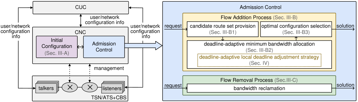
Figure 2: Online admission control framework in a fully centralized model.

II-B NC-based Worst-Case Delay Analysis for TAS/ATS+CBS

The network calculus (NC)-based worst-case delay analysis for TSN/ATS+CBS has been provided [23]. In network calculus theory [24], the arrival curve $\alpha(t)$ constrains the data bits accumulated from incoming flows over any time interval, while the service curve $\beta(t)$ represents the minimum processing capacity of the service element over any time interval. The maximum horizontal distance between the two curves is the worst-case delay bound at the egress port. With the assistance of ATS reshaping, each AVB flow $f$ conforms to a committed burst $b_{f}=l_{f}$ and a committed rate $\rho_{f}=l_{f}/p_{f}$ at each egress port along its route. Then, the arrival curve of the aggregate flows of AVB class $i$ before the egress port $(u,v)$ is

$$\alpha_{i}^{(u,v)}(t)=\sum_{f\in\mathcal{F}_{i}^{(u,v)}}(\rho_{f}\cdot t+b_{f}),$$ (1)

where $\mathcal{F}_{i}^{(u,v)}$ is the subset of AVB flows $\mathcal{F}$ of class $i$ at egress port $(u,v)$. The CBS service curve [14] for AVB class $i$ at egress port $(u,v)$ is

$$\beta_{i}^{(u,v)}(t)=idSl_{i}^{(u,v)}\left[t-\frac{\sum_{j=1}^{i-1}(sdSl_{j}^{(u,v)}\cdot\frac{l_{j}^{\max}}{C})-l_{>i}^{\max}}{\sum_{j=1}^{i-1}idSl_{j}^{(u,v)}-C}\right]^{+},$$ (2)

where $sdSl_{i}^{(u,v)}=idSl_{i}^{(u,v)}-C$ is the send slope for AVB class $i$ at egress port $(u,v)$, $l_{i}^{\max}$ is the maximum frame size of AVB class $i$, and $l_{>i}^{\max}=\max_{j>i}\{l_{j}^{\max},l_{\rm BE}^{\max}\}$ is the maximum frame size of traffic with lower priorities than $i$. The upper bound of the worst-case delay for any flow $f\in\mathcal{F}_{i}^{(u,v)}$ queuing at egress port $(u,v)$ is the maximum horizontal distance between the arrival curve $\alpha_{i}^{(u,v)}(t)$ and the service curve $\beta_{i}^{(u,v)}(t)$. Furthermore, it is proven in [25] that ATS shaping after a first-in, first-out (FIFO) system does not add extra delays to the worst-case delay of the combination. Therefore, AVB flows do not experience extra worst-case delays in the reshaping queues before ATS. The worst-case delay bound $H_{i}^{(u,v)}$ for AVB class $i$ queuing at egress port $(u,v)$ can ultimately be expressed as

$$H_{i}^{(u,v)}=\frac{\sum_{f\in\mathcal{F}_{i}^{(u,v)}}b_{f}}{idSl_{i}^{(u,v)}}+\frac{l^{\max}}{C}+\frac{(i-1)l^{\max}}{C-\sum_{j=1}^{i-1}idSl_{j}^{(u,v)}},$$ (3)

where $l_{i}^{\max}$ is simplified to $l^{\max}$, representing the maximum frame size in the network, to reduce the complexity caused by updating $l_{i}^{\max}$ during online processing.

III Online Admission Control Framework

Online admission control is a procedure that, based on available resources, determines whether to admit a flow addition request and configures resources if admitted; it also reclaims resources for future traffic access once a flow is removed. In the online admission control method for time-critical ET traffic, the main challenge is rapidly providing configurations that meet the end-to-end delay requirements while optimizing the utilization of leftover network resources for future access needs. Since cascading bursts among flows can cause the addition of a new flow to impact the real-time performance of all existing flows throughout the network, avoiding such cascades can greatly reduce the reconfiguration domain. Therefore, we recommend the TSN/ATS+CBS architecture, which employs ATS to prevent burst cascades. It also uses CBS to enable flexible bandwidth $(idSl)$ allocation for different AVB traffic classes. Moreover, it is revealed that with increasing traffic loads, the combined use of ATS and CBS outperforms CBS alone in terms of worst-case delay [26].

The online admission control framework, implemented in a fully centralized model that includes Centralized User Configuration (CUC) and Centralized Network Configuration (CNC), is shown in Fig. 2. The CUC is responsible for obtaining application requests from end systems (ES) and forwarding them to the CNC. The CNC manages the initial network configuration and performs admission control operations, including the flow addition process and the flow removal process. For a new flow addition request, the flow addition process determines whether there is an optimal configuration, including routing and bandwidth allocation, that meets the deadlines of both new and existing flows. Our proposed admission control framework, leveraging a novel prior performance analysis model [21], enables the process to not only reduce admission time by avoiding iterative optimization and ex-post verification but also improve network bandwidth utilization by effectively balancing the residual bandwidth. For a flow removal request, the flow removal process provides the configuration to reclaim bandwidth for future flow access. The configurations modified during the admission control operations will replace the initial configuration in the CNC and be distributed to all switches via protocols such as NETCONF [27].

III-A Initial Configuration Before Admission Control

To improve the utilization of residual bandwidth resources for future access needs while ensuring the deadlines of time-critical ET traffic, we employ the latest QoS-based minimum bandwidth allocation analytical method [21] to provide the initial network configuration. The configuration process is divided into two stages. The first stage is to determine the local deadlines for each class at every egress port using a decomposition method, such as the one described in [21]. This stage is represented as

$$Stage\ 1:\forall(u,v)\in\mathcal{L},i\in[1,N_{\rm AVB}]:\quad\quad\quad\quad\quad\quad\quad\quad\quad\quad\quad\quad$$ (4)

$$\quad\quad\quad\quad\quad\quad\qquad D_{i}^{(u,v)}=\min_{f\in\mathcal{F}_{i}^{(u,v)}}\Big{\{}D_{f}^{(u,v)}\Big{\}},$$

where

$$\sum_{(u,v)\in r_{f}}D_{f}^{(u,v)}\leq D_{f}^{\rm E2E}.$$ (5)

$D_{i}^{(u,v)}$ denotes the local deadline for class $i$ at egress port $(u,v)$, $r_{f}$ denotes the route of flow $f$, and $D_{f}^{(u,v)}$ denotes the local deadline for flow $f$ at egress port $(u,v)\in r_{f}$, as obtained by the decomposition method in [21]. The local deadlines for each flow ensure that the worst-case delay along the route does not exceed its end-to-end deadline. In order to meet the strictest deadlines, the local deadline for each class at every egress port is set to the minimum of the local deadlines for all flows within that class at that port. The second stage is to allocate the minimum bandwidth for each class at every egress port to satisfy the local deadlines. This stage is defined as

$$Stage\ 2:\forall(u,v)\in\mathcal{L},i\in[1,N_{\rm AVB}]:$$ (6)

$$idSl_{i}^{(u,v)}=$$

$$\max\Bigg{\{}\underbrace{\frac{\sum_{f\in\mathcal{F}_{i}^{(u,v)}}b_{f}}{D_{i}^{(u,v)}-\frac{l^{\max}}{C}-\frac{(i-1)l^{\max}}{C-\sum_{j=1}^{i-1}idSl_{j}^{(u,v)}}}}_{first},\underbrace{\sum_{f\in\mathcal{F}_{i}^{(u,v)}}\rho_{f}}_{second}\Bigg{\}},$$

where the first term determines the minimum bandwidth required to satisfy the local deadline $D_{i}^{(u,v)}$ for each class $i\in[1,N_{\rm AVB}]$ at every egress port $(u,v)\in\mathcal{L}$, as proven in [21], the second term maintains network stability. Note that since we leverage ATS in the admission control architecture to avoid burst cascades, the burst size $b_{f}$ and long-term rate $\rho_{f}$ of flow $f$ on the egress port $(u,v)$ in Eq. (LABEL:MiniBand) remain the same as they were when sent from the source ES. Additionally, Eq. (LABEL:MiniBand) reveals that the minimum bandwidth allocation to lower priority classes depends on the allocation results of higher priority classes. Therefore, the minimum bandwidth is allocated from high priority to low priority.

For the initial configuration in the CNC, we store the tuple, route $r_{f}$, and local deadlines $D_{f}^{(u,v)}$ along the $r_{f}$ for each flow $f$. Additionally, we need to store the local deadline $D_{i}^{(u,v)}$ and bandwidth allocation $idSl_{i}^{(u,v)}$ for each class $i$ at every egress port $(u,v)$. Subsequently, we will explore how to perform online admission control relying on the initial configuration, using the prior performance analysis model [21]. We aim to maximize the number of admitted flows with minimized bandwidth usage while ensuring that the deadline requirements of both new and initial flows are met, by quickly and dynamically allocating and reclaiming bandwidth resources.

III-B Flow Addition Process

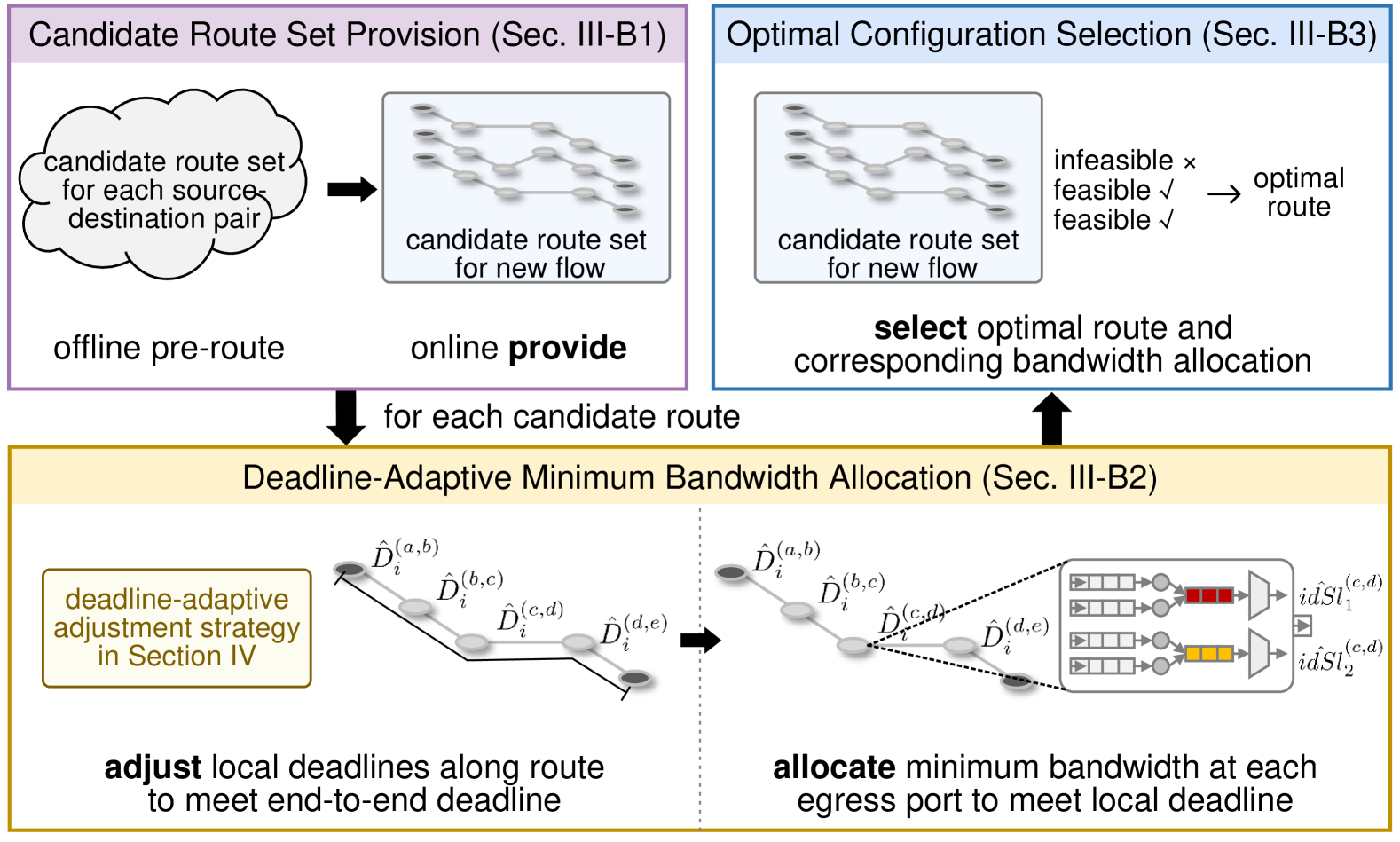
Figure 3: Flow Addition Process.

When a new flow $f^{+}$ requests to be added, the flow addition process in our admission control framework evaluates, based on the available bandwidth, whether to admit the request and how to provide configuration if admitted. The configuration, including the route and allocated bandwidth, should satisfy the end-to-end deadline requirements of both the new and existing flows while maximizing the utilization of remaining network resources. The specific procedure of the flow addition process is shown in Fig. 3. Given that online routing is time-consuming, the candidate route set for each source-destination pair is generated offline through pre-routing. During the online phase, a new flow is assigned the corresponding candidate route set based on its source ES and destination ES (Section III-B1). Subsequently, the process provides a deadline-adaptive minimum bandwidth allocation scheme for each route within the candidate set of the new flow (Section III-B2). This scheme aims to quickly meet end-to-end deadline requirements while adaptively balancing the residual bandwidth (as outlined in Section 4). Finally, this process evaluates all the routes within the candidate set of the new flow along with their corresponding bandwidth allocation schemes and selects the optimal configuration (Section III-B3). Detailed discussions will be provided as follows.

III-B1 Candidate Route Set Provision

When a flow requests to be added, we first need to provide it with a route. To avoid the complexity of online routing, we pre-route a set of candidate routes for each source-destination pair, enabling efficient online retrieval. We use the k-shortest path algorithm [28] to generate the candidate route set ${\mathcal{R}(s,d)}$ for each source-destination pair, where $s$ and $d$ are end-systems. We choose the k-shortest path algorithm for two main reasons. On the one hand, we aim to select shorter routes to achieve larger local deadlines for each egress port along the route. This ensures that more residual bandwidth is reserved according to Eq. (4), providing greater flexibility in bandwidth allocation while maintaining end-to-end deadline performance (Section III-B2). On the other hand, providing k routes offers greater flexibility in route selection, thereby better balancing the remaining network bandwidth (Section III-B3). During the online phase, a new flow $f^{+}$ is assigned the corresponding candidate route set $\mathcal{R}(s_{f^{+}},d_{f^{+}})$ based on its source ES $s_{f^{+}}$ and destination ES $d_{f^{+}}$.

III-B2 Deadline-Adaptive Minimum Bandwidth Allocation

When a new flow $f^{+}$ is assigned to a route $r_{f^{+}}\in\mathcal{R}(s_{f^{+}},d_{f^{+}})$, we need to find a bandwidth allocation scheme ($\hat{idSl}$) that meets the end-to-end deadline requirements. We perform the analysis based on the prior performance analysis model [21], which includes Stage 1 with Eqs. (4) and (5) and Stage 2 with Eq. (LABEL:MiniBand). Our main focus is to adjust the local deadlines in Stage 1 to meet the deadline of the new flow. In order to minimize changes to the initial configuration, we adjust the local deadlines only at the egress ports along the route $r_{f^{+}}$ of the new flow with the assistance of ATS rather than reallocating local deadlines for all egress ports in the network. Once the local deadlines are set, we can directly apply the method from Stage 2 to calculate the bandwidth allocation scheme for adding flow $f^{+}$ along route $r_{f^{+}}$.

Theorem 1.

To meet the end-to-end deadline $D_{f^{+}}^{\rm E2E}$ of the new flow $f^{+}$ of class $i$, the adjusted local deadline $\hat{D}_{i}^{(u,v)}$ for class $i$ at egress port $(u,v)$ along the route $r_{f^{+}}$ is

$$\hat{D}_{i}^{(u,v)}=\begin{cases}D_{i}^{(u,v)},&\sum\limits_{(u,v)\in r_{f^{+}}}D_{i}^{(u,v)}\leq D_{f^{+}}^{\rm E2E}\\ \hat{D}_{i}^{(u,v)}\ \rm from\ Alg.1,&\sum\limits_{(u,v)\in r_{f^{+}}}D_{i}^{(u,v)}>D_{f^{+}}^{\rm E2E}\\ \end{cases},$$ (7)

where $D^{(u,v)}_{i}$ is the initial local deadline for class $i$ at egress port $(u,v)$ as defined in Eq. (4), and $D^{\rm E2E}_{f^{+}}$ is the end-to-end deadline of the new flow $f^{+}$.

Proof.

There are two cases for adjusting the local deadlines. When the sum of the initial local deadlines $D^{(u,v)}_{i}$ along the route $r_{f^{+}}$ meets the end-to-end deadline of the new flow $f^{+}$, i.e., $\sum_{(u,v)\in r_{f^{+}}}D_{i}^{(u,v)}\leq D_{f^{+}}^{\rm E2E}$, there is no need for further adjustments to the local deadlines to meet the end-to-end deadline requirements. As a result, the local deadline $D_{i}^{(u,v)}$ remains unchanged, i.e., $\hat{D}^{(u,v)}_{i}=D^{(u,v)}_{i}$. When the sum of the initial local deadlines $D^{(u,v)}_{i}$ along the route $r_{f^{+}}$ exceeds the end-to-end deadline of the new flow $f^{+}$, i.e., $\sum_{(u,v)\in r_{f^{+}}}D_{i}^{(u,v)}>D_{f^{+}}^{\rm E2E}$, $D^{(u,v)}_{i}$ at each egress port along the route $r_{f^{+}}$ needs to be reduced to meet the end-to-end deadline of new flow $f^{+}$. However, adjusting $D^{(u,v)}_{i}$ is not straightforward, as reducing these local deadlines will affect the distribution of the remaining bandwidth across different egress ports in the network, requiring careful balancing to optimize resource utilization. We determine $\hat{D}_{i}^{(u,v)}$ using Algorithm 1, specifically discussed in Section 4, by employing a deadline-adaptive local deadline adjustment strategy to balance the remaining bandwidth resources. $\hfill\blacksquare$

After obtaining the adjusted local deadlines $\hat{D}^{(u,v)}_{i}$ for class $i$ at egress port $(u,v)$ along the route $r_{f^{+}}$ in Theorem 1, the corresponding bandwidth allocation $\hat{idSl}_{j}^{(u,v)}\ (j\in[1,N_{\rm AVB}],(u,v)\in\mathcal{L})$ for adding flow $f^{+}$ on route $r_{f^{+}}$ is determined by substituting $\mathcal{F}$ with $\mathcal{F}\cup{f^{+}}$ and $D_{i}^{(u,v)}$ with $\hat{D}_{i}^{(u,v)}$ in Eq. (LABEL:MiniBand). According to Eq. (LABEL:MiniBand), the addition of flow $f^{+}$ only affects the bandwidth allocation for classes with priorities equal to or lower than that of flow $f^{+}$ on route $r_{f^{+}}$, without causing large-scale reconfiguration. Additionally, the local deadline $D_{f^{+}}^{(u,v)}$ for new flow $f^{+}$ along the route $r_{f^{+}}$ is assigned the value of $\hat{D}_{i}^{(u,v)}$, ensuring that $\sum_{(u,v)\in r_{f^{+}}}D_{f^{+}}^{(u,v)}\leq D_{f^{+}}^{\rm E2E}$ is satisfied in accordance with Eq. (5) from Stage 1.

III-B3 Optimal Configuration Selection

Finally, we obtain the optimal configuration by selecting the optimal route $r_{f^{+}}^{\rm opt}$ from the $k$ candidate routes $r_{f^{+}}\in\mathcal{R}(s_{f^{+}},d_{f^{+}})$ based on the corresponding bandwidth allocation ($\hat{idSl}$) obtained from Section III-B2. Initially, we need to evaluate the feasibility of each candidate route, which is determined by two conditions. The first condition is that feasible local deadlines can be provided by Eq. (7). The second condition is that the sum of bandwidth allocations at each egress port does not exceed the upper limit $idSl^{\max}$, i.e., $\sum_{i=1}^{N_{\rm AVB}}\hat{idSl}_{i}^{(u,v)}\leq idSl^{\max}$. If at least one feasible route exists, we will select the optimal one to admit the new flow $f^{+}$ using the following method. If no feasible route exists, it is impossible to find a route that meets the end-to-end deadline requirement of the new flow, and the request to add the new flow will be rejected.

The optimal route $r_{f^{+}}^{\rm opt}$ is defined as

$$r_{f^{+}}^{\rm opt}=\arg\min_{r_{f^{+}}\in\mathcal{R}(s_{f^{+}},d_{f^{+}})\land\rm feasible}\{cost(r_{f^{+}})\},$$ (8)

and

$$cost(r_{f^{+}})=$$ (9)

$$\sum_{(u,v)\in\mathcal{L}}\left(\frac{1}{idSl^{\max}-\sum_{i=1}^{N_{\rm AVB}}\hat{idSl}_{i}^{(u,v)}}-\frac{1}{idSl^{\max}}\right)^{2},$$

where $cost(r_{f^{+}})$ represents the network cost associated with the bandwidth allocation scheme for adding flow $f^{+}$ along route $r_{f^{+}}$, $1/(idSl^{\max}-\sum_{i=1}^{N_{\rm AVB}}\hat{idSl}_{i}^{(u,v)})$ is the actual egress port cost considering the residual bandwidth, and $1/idSl^{\max}$ is the minimum possible egress port cost when no bandwidth is utilized. The network cost $cost(r_{f^{+}})$ is determined by calculating the difference between the actual egress port cost and the minimum possible egress port cost, squaring this difference, and summing the results of all egress ports. When the residual bandwidth of an egress port is low, the network cost $cost(r_{f^{+}})$ rises sharply, indicating bottleneck egress ports nearing resource exhaustion, potentially hindering future flow admissions. Consequently, we can select the optimal route $r_{f^{+}}^{\rm opt}$ by minimizing the network cost as defined in Eq. (9), which balances the residual bandwidth. This helps avoid bottleneck egress ports caused by resource exhaustion, thereby enhancing the capacity of the network to accommodate future traffic.

III-C Flow Removal Process

After removing flow $f^{-}$, the flow removal process needs to provide a bandwidth allocation scheme ($\check{idSl}$) to reclaim bandwidth resources for future traffic access. First, we remove the local deadlines related to flow $f^{-}$ of class $i$. The adjusted local deadline $\check{D}_{i}^{(u,v)}$ for class $i$ at egress port $(u,v)\in r_{f^{-}}$ is

$$\check{D}_{i}^{(u,v)}=\min_{f\in(\mathcal{F}\setminus\{f^{-}\})_{i}^{(u,v)}}\Big{\{}D_{f}^{(u,v)}\Big{\}}.$$ (10)

Subsequently, the adjusted bandwidth allocation $\check{idSl}_{j}^{(u,v)}\ (j\in[1,N_{\rm AVB}],(u,v)\in\mathcal{L})$ for removing flow $f^{-}$ is determined by substituting $\mathcal{F}$ with $\mathcal{F}\setminus\{f^{-}\}$ and $D_{i}^{(u,v)}$ with $\check{D}_{i}^{(u,v)}$ in Eq. (LABEL:MiniBand). Similar to flow addition, the bandwidth reclamation after removing flow $f^{-}$ affects only the bandwidth allocation for classes with priorities equal to or lower than that of flow $f^{-}$ on route $r_{f^{-}}$, without the need for large-scale reconfiguration.

IV Deadline-Adaptive Local Deadline Adjustment Strategy

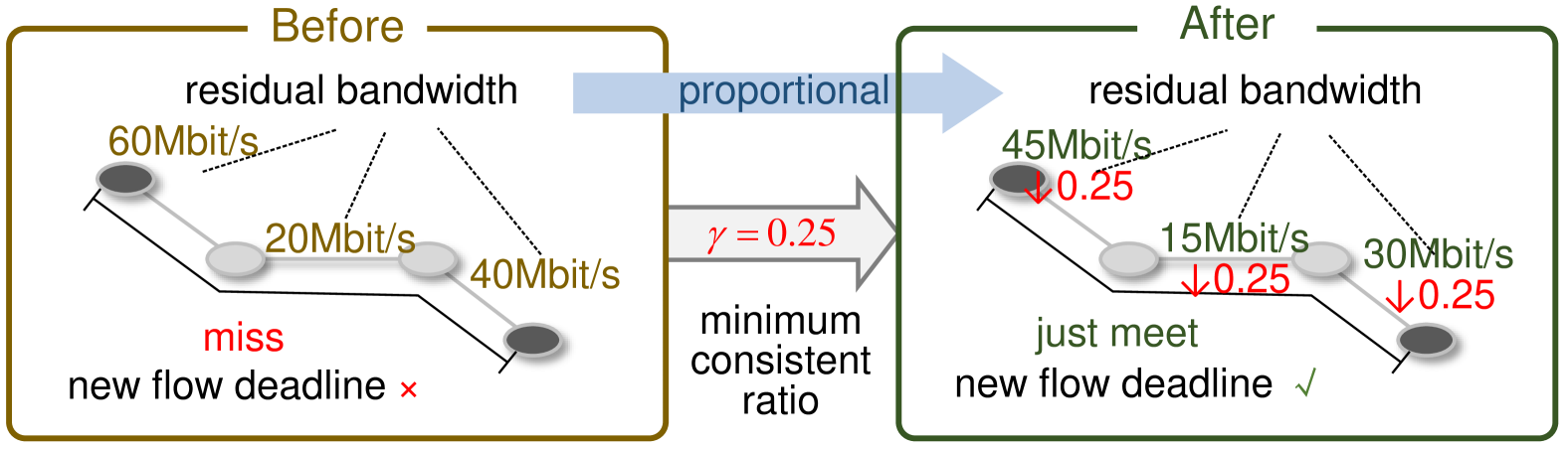
Figure 4: An example of local deadlines adjusted by minimum consistent ratio $\gamma=0.25$ to just meet the new flow deadline.

In Section III-B2, if the sum of the initial local deadlines $D_{i}^{(u,v)}$ in Eq. (4) along route $r_{f^{+}}$ exceeds the end-to-end deadline $D_{f^{+}}^{\rm E2E}$ of the new flow $f^{+}$ of class $i$, $D_{i}^{(u,v)}$ should be reduced to meet the end-to-end deadline. Some studies [29] have directly modified local deadlines $D_{i}^{(u,v)}$ by adjusting them either equally or proportionally, ensuring that the adjusted local deadlines $\hat{D}_{i}^{(u,v)}$ meet the end-to-end deadline. Although these methods are relatively simple, they do not address residual bandwidth balancing, which can lead to early resource exhaustion at bottleneck egress ports. Therefore, we propose a deadline-adaptive strategy that adjusts local deadlines in a way that balances residual bandwidth at the egress ports. It ensures that the extra bandwidth needed at each egress port to meet the newly adjusted local deadline is allocated in proportion to the available residual bandwidth at each port, thereby balancing residual bandwidth across all egress ports. Furthermore, the strategy intends to minimize the extra bandwidth needed to meet the newly adjusted local deadline, ensuring that more residual bandwidth remains available for future traffic access. According to Eq. (LABEL:MiniBand), a larger bandwidth allocation is required to achieve a smaller adjusted local deadline. Therefore, the strategy aims to determine the minimum ratio of extra bandwidth to available residual bandwidth, represented by a minimum consistent ratio $\gamma$ across all ports, in cases where the end-to-end deadline of the new flow is just met. Fig. 4 shows an example where the local deadlines along the route of the new flow are adjusted by the minimum consistent ratio $\gamma=0.25$ to just meet the end-to-end deadline of the new flow. The determination of the minimum consistent ratio $\gamma$ and the calculation of adjusted local deadlines $\hat{D}_{i}^{(u,v)}$ are provided by the following algorithm.

Algorithm 1 Local Deadline Adjustment Algorithm

1: Input: $f^{+}$: flow for addition, $r_{f^{+}}$: candidate route;

2: Output: $\{\hat{D}_{i}^{(u,v)}\}_{(u,v)\in r_{f^{+}}}$: adjusted local deadlines for class

3:$i$ along route $r_{f^{+}}$;

4:for $(u,v)\in r_{f^{+}}$ do

5:  $R^{(u,v)}\leftarrow\texttt{CalResBand}()$

6:end for

7:for $(u,v)\in r_{f^{+}}$ do

8:  $\hat{D}_{i}^{(u,v),\min}\leftarrow\texttt{MapBand2D}(R^{(u,v)})$

9:end for

10:if $\sum_{(u,v)\in r_{f^{+}}}\hat{D}_{i}^{(u,v),\min}\leq D_{f^{+}}^{\rm E2E}$ then

11:  $\gamma\leftarrow 1$, $\delta\leftarrow 1$, $slack\leftarrow-1$

12:  while $slack\neq 0$ do

13:   for $(u,v)\in r_{f^{+}}$ do

14:     $\hat{D}_{i}^{(u,v)}\leftarrow\texttt{MapBand2D}(\gamma\cdot R^{(u,v)})$

15:   end for

16:   $slack\leftarrow D_{f^{+}}^{\rm E2E}-\sum_{(u,v)\in r_{f^{+}}}\hat{D}_{i}^{(u,v)}$

17:   $\delta\leftarrow\delta/2$

18:   $\gamma\leftarrow(slack>0)?\gamma-\delta:\gamma+\delta$

19:  end while

20:else

21:  $\{\hat{D}_{i}^{(u,v)}\}_{(u,v)\in r_{f^{+}}}\leftarrow\texttt{infeasible}$

22:end if

Algorithm: We propose a local deadline adjustment algorithm, with its pseudo-code presented in Algorithm 1. The algorithm first calculates the available residual bandwidth $R^{(u,v)}$ for each egress port $(u,v)\in r_{f^{+}}$ using the CalResBand function described in Section IV-A (lines 1-3). Then, the algorithm calculates the extra bandwidth $\gamma\cdot R^{(u,v)}$ needed to meet the end-to-end deadline of the new flow, thereby reducing the local deadlines $D_{i}^{(u,v)}$ along the route $r_{f^{+}}$ by allocating this extra bandwidth. As indicated in Eq. (LABEL:MiniBand), achieving a smaller adjusted local deadline requires a larger bandwidth allocation. Initially, assuming all available residual bandwidth $R^{(u,v)}$ is used as extra bandwidth, the algorithm calculates the minimum possible adjusted local deadlines $\hat{D}_{i}^{(u,v),\rm min}$ for each egress port $(u,v)\in r_{f^{+}}$ using the MapBand2D function described in Section IV-B (lines 4-6). If the sum of the minimum possible adjusted local deadlines $\hat{D}_{i}^{(u,v),\rm min}$ along the route $r_{f^{+}}$ cannot meet the end-to-end deadline $D_{f^{+}}^{\rm E2E}$ of the new flow $f^{+}$, it indicates that no feasible local deadline adjustment can exist (lines 18). Conversely, if the sum is smaller than the end-to-end deadline $D_{f^{+}}^{\rm E2E}$ of the new flow $f^{+}$, it means that a smaller extra bandwidth than $R^{(u,v)}$ can be found to meet $D_{f^{+}}^{\rm E2E}$. The algorithm seeks to find the minimum extra bandwidth needed to adjust the local deadlines to meet $D_{f^{+}}^{\rm E2E}$ (lines 8-16). Since Eq. (LABEL:MiniBand) indicates that a smaller adjusted local deadline requires a larger bandwidth allocation, the minimum extra bandwidth is achieved by maximizing the adjusted local deadlines so that their sum just meets $D_{f^{+}}^{\rm E2E}$. In order to achieve this, the algorithm performs a binary search to determine the minimum consistent ratio $\gamma$ $(0<\gamma\leq 1)$ such that the sum of the adjusted local deadlines equals $D_{f^{+}}^{\rm E2E}$. In the binary search process, $\gamma$ represents the consistent ratio of extra bandwidth to available residual bandwidth, $\delta$ indicates the adjustment to $\gamma$, and $slack$, initialized to -1, denotes the difference between the end-to-end deadline of the new flow and the sum of the adjusted local deadlines. In each iteration, the MapBand2D function calculates the adjusted local deadlines $\hat{D}_{i}^{(u,v)}$ based on the extra bandwidth $\gamma\cdot R^{(u,v)}$. The $slack$ is then computed, and $\gamma$ is adjusted by $\delta$ based on whether $slack$ is positive or negative, bringing it closer to 0. The binary search process ends when $slack=0$, at which point the adjusted local deadlines $\{\hat{D}_{i}^{(u,v)}\}_{(u,v)\in r_{f^{+}}}$ are obtained. The detailed implementations of the CalResBand and MapBand2D functions are as follows.

IV-A Port-Level Calculating Residual Bandwidth

In line 2 of Algorithm 1, the CalResBand function calculates the available residual bandwidth $R^{(u,v)}$ at each egress port $(u,v)$ along the route $r_{f^{+}}$ of the new flow $f^{+}$, represented as

$$R^{(u,v)}=idSl^{\max}-\sum_{j=1}^{N_{\rm AVB}}\bar{idSl}_{j}^{(u,v)},$$ (11)

where $\bar{idSl}_{j}^{(u,v)}$ represents the already allocated bandwidth that satisfies the initial local deadlines $D_{i}^{(u,v)}$ in Eq. (4). Compared to $idSl_{j}^{(u,v)}$ in Eq. (LABEL:MiniBand), which only considers the already admitted flow set $\mathcal{F}$, $\bar{idSl}_{j}^{(u,v)}\ (j\in[1,N_{\rm AVB}])$ additionally includes the new flow $f^{+}$, and is expressed as

$$\bar{idSl}_{j}^{(u,v)}=\frac{\sum_{f\in(\mathcal{F}\cup\{f^{+}\})_{j}^{(u,v)}}b_{f}}{D_{j}^{(u,v)}-\frac{l^{\max}}{C}-\frac{(j-1)l^{\max}}{C-\sum_{k=1}^{j-1}\bar{idSl}_{k}^{(u,v)}}},$$ (12)

by replacing $\mathcal{F}$ with $\mathcal{F}\cup{f^{+}}$ in the first term of Eq. (LABEL:MiniBand). As described in Algorithm 1, in order to balance the residual bandwidth across egress ports, the available residual bandwidth $R^{(u,v)}$ is used to determine the extra bandwidth needed at each egress port to adjust the local deadline $D_{i}^{(u,v)}$.

IV-B Port-Level Mapping Extra Bandwidth to Deadline

In lines 5 and 11 of Algorithm 1, the MapBand2D function computes the adjusted local deadlines $\hat{D}_{i}^{(u,v)}$ when the extra bandwidth is $\gamma\cdot R^{(u,v)}\ (0<\gamma\leq 1)$. The implementation of the MapBand2D function is detailed in Theorem 2.

Theorem 2.

For each egress port $(u,v)\in r_{f^{+}}$, the adjusted local deadline $\hat{D}_{i}^{(u,v)}$ for class $i$, corresponding to the extra bandwidth $\gamma\cdot R^{(u,v)}\ (0<\gamma\leq 1)$, is given by

$$\hat{D}_{i}^{(u,v)}=\frac{\sum_{f\in(\mathcal{F}\cup\{f^{+}\})_{i}^{(u,v)}}b_{f}}{\bar{idSl}_{i}^{(u,v)}+\Phi_{i}}+\frac{l^{\max}}{C}+\frac{(i-1)l^{\max}}{C-\sum_{j=1}^{i-1}\bar{idSl}_{j}^{(u,v)}},$$ (13)

where $\bar{idSl}_{i}^{(u,v)}$ represents the already allocated bandwidth for class $i$ at egress port $(u,v)$ in Eq. (12), and $\Phi_{i}$ denotes the extra bandwidth allocated to class $i$. The extra bandwidth $\gamma\cdot R^{(u,v)}$ equals the sum of the extra bandwidth $\Phi_{k}\ (k\in[i,N_{\rm AVB}])$ allocated from class $i$ to class $N_{\rm AVB}$, given by

$$\sum_{k=i}^{N_{\rm AVB}}\Phi_{k}=\gamma\cdot R^{(u,v)}.$$ (14)

The value of $\Phi_{i}$ in Eq. (13) is determined by the recursive relationship $\sum_{k=i}^{j-1}\Phi_{k}=g(\sum_{k=i}^{j}\Phi_{k})$, as stated in Lemma 1, with the initial term being Eq. (14).

Proof.

For each egress port $(u,v)\in r_{f^{+}}$, the extra bandwidth $\gamma\cdot R^{(u,v)}$, which is based on the already allocated bandwidth $(\bar{idSl})$ in Eq. (12), is used to adjust the local deadline $D_{i}^{(u,v)}$ for class $i$ to a lower value. According to Eq. (12), reducing the local deadline $D_{i}^{(u,v)}$ for class $i$ not only requires allocating extra bandwidth $\Phi_{i}$ to the target class $i$ but also necessitates allocating extra bandwidth $\Phi_{j}$ to all lower-priority classes $j\ (j\in[i+1,N_{\rm AVB}])$ to ensure that their initial local deadlines $D_{j}^{(u,v)}$ remain unaffected by the extra bandwidth allocated to higher-priority classes. Therefore, the extra bandwidth $\gamma\cdot R^{(u,v)}$ is divided among the classes from $i$ to $N_{\rm AVB}$, i.e., $\sum_{k=i}^{N_{\rm AVB}}\Phi_{k}=\gamma\cdot R^{(u,v)}$. The extra bandwidth $\Phi_{i}$ for class $i$ is obtained through a recursive relationship, which derives $\sum_{k=i}^{j-1}\Phi_{k}$ from $\sum_{k=i}^{j}\Phi_{k}\ (j\in[i+1,N_{\rm AVB}])$, using the known sum $\sum_{k=i}^{N_{\rm AVB}}\Phi_{k}$. To ensure that the initial local deadline $D_{j}^{(u,v)}$ for class $j$ is met, the recursive relationship should satisfy $\sum_{k=i}^{j-1}\Phi_{k}=g(\sum_{k=i}^{j}\Phi_{k})$, as proved in Lemma 1. Therefore, based on the extra bandwidth $\Phi_{i}$ for class $i$ obtained from the recursive relationship, the adjusted local deadline $\hat{D}_{i}^{(u,v)}$ is give in Eq. (13), by replacing $\bar{idSl}_{i}^{(u,v)}$ with $\bar{idSl}_{i}^{(u,v)}+\Phi_{i}$ and solving for $\hat{D}_{i}^{(u,v)}$ in Eq. (12). $\hfill\blacksquare$

Lemma 1.

To ensure that the initial local deadline $D_{j}^{(u,v)}$ for the low-priority class $j\ (j\in[i+1,N_{\rm AVB}])$ is met when adjusting the local deadline $D_{i}^{(u,v)}$ for class $i$, the recursive relationship to obtain $\sum_{k=i}^{j-1}\Phi_{k}$ from the known $\sum_{k=i}^{j}\Phi_{k}$ should satisfy

$$\sum_{k=i}^{j-1}\Phi_{k}=g(\sum_{k=i}^{j}\Phi_{k})=\frac{-\xi-\sqrt{\xi^{2}-4\cdot\eta\cdot\zeta}}{2\cdot\eta},$$ (15)

where

$$\eta=1+\frac{(C-\sum_{k=1}^{j-1}\bar{idSl}_{k}^{(u,v)})\sum_{f\in(\mathcal{F}\cup\{f^{+}\})_{j}^{(u,v)}}b_{f}}{(j-1)l^{\max}\cdot\bar{idSl}_{j}^{(u,v)}},$$ (16)

$$\xi=-\eta\sum_{k=i}^{j}\Phi_{k}-(\eta-1)(C-\sum_{k=i}^{j-1}\bar{idSl}_{k}^{(u,v)})-\bar{idSl}_{j}^{(u,v)},$$ (17)

$$\zeta=(\eta-1)(C-\sum_{k=1}^{j-1}\bar{idSl}_{k}^{(u,v)})\sum_{k=i}^{j}\Phi_{k},$$ (18)

where $\bar{idSl}_{k}^{(u,v)}$ is the already allocated bandwidth for class $k$ at egress port $(u,v)$ in Eq. (12).

Proof.

The known $\sum_{k=i}^{j}\Phi_{k}$ can be split into two parts, $\sum_{k=i}^{j-1}\Phi_{k}$ and $\Phi_{j}$, with $\sum_{k=i}^{j}\Phi_{k}=\sum_{k=i}^{j-1}\Phi_{k}+\Phi_{j}$. We first determine the relationship between $\sum_{k=i}^{j-1}\Phi_{k}$ and $\Phi_{j}$ to meet the initial local deadline $D_{j}^{(u,v)}$ for low-prority class $j$. According to Theorem 2, to ensure the initial local deadline $D_{j}^{(u,v)}$, extra bandwidth $\Phi_{j}$ for class $j$ is needed. The new bandwidth allocation for class $j$ to meet its initial local deadline $D_{j}^{(u,v)}$, when the extra bandwidth $\sum_{k=i}^{j-1}\Phi_{k}$ is allocated to classes from $i$ to $j-1$, is obtained by replacing $\sum_{k=1}^{j-1}\bar{idSl}_{k}^{(u,v)}$ with $\sum_{k=1}^{j-1}\bar{idSl}_{k}^{(u,v)}+\sum_{k=i}^{j-1}\Phi_{k}$ in Eq. (12). The difference between the new bandwidth allocation and the already allocated bandwidth $\bar{idSl}_{j}$ is the extra bandwidth $\Phi_{j}$ needed for class $j$. Thus, the relationship between $\sum_{k=i}^{j-1}\Phi_{k}$ and $\Phi_{j}$ to meet the initial local deadline $D_{j}^{(u,v)}$ is

$$\Phi_{j}=\frac{\sum_{f\in(\mathcal{F}\cup\{f^{+}\})_{j}^{(u,v)}}b_{f}}{D_{j}^{(u,v)}-\frac{l^{\max}}{C}-\frac{(j-1)l^{\max}}{C-(\sum_{k=1}^{j-1}\bar{idSl}_{k}^{(u,v)}+\sum_{k=i}^{j-1}\Phi_{k})}}-\bar{idSl}_{j}^{(u,v)}.$$ (19)

We then derive the relationship between $\sum_{k=i}^{j-1}\Phi_{k}$ and $\sum_{k=i}^{j}\Phi_{k}$. We use $\sum_{k=i}^{j}\Phi_{k}=\sum_{k=i}^{j-1}\Phi_{k}+\Phi_{j}$ and combine it with the relationship between $\sum_{k=i}^{j-1}\Phi_{k}$ and $\Phi_{j}$ from Eq. (19) to eliminate $\Phi_{j}$. Additionally, to reduce the number of symbols used, we eliminate $D_{j}^{(u,v)}$ by solving for it using Eq. (12) and substituting it accordingly. Thus, the relationship between $\sum_{k=i}^{j-1}\Phi_{k}$ and $\sum_{k=i}^{j}\Phi_{k}$ to meet the initial local deadline $D_{j}^{(u,v)}$ for low-priority class $j$ is

$$\eta(\sum_{k=i}^{j-1}\Phi_{k})^{2}+\xi(\sum_{k=i}^{j-1}\Phi_{k})+\zeta=0,$$ (20)

where the coefficients $\eta$, $\xi$, and $\zeta$ associated with $\sum_{k=i}^{j}\Phi_{k}$ are given in Eqs. (16), (17) and (18), respectively. Then, we attempt to find the solution for $\sum_{k=i}^{j-1}\Phi_{k}$ in Eq. (20) within the feasible interval $[0,\sum_{k=i}^{j}\Phi_{k}]$, since $\sum_{k=i}^{j-1}\Phi_{k}$ cannot exceed $\sum_{k=i}^{j}\Phi_{k}$. We let $f(x)=\eta x^{2}+\xi x+\zeta$, and observe that $\eta>0$, $f(0)=\zeta\geq 0$, and $f(\sum_{k=i}^{j}\Phi_{k})=-\bar{idSl}_{j}^{(u,v)}\cdot\sum_{k=i}^{j}\Phi_{k}\leq 0$. Therefore, of the two solutions to Eq. (20), one lies within the interval $[0,\sum_{k=i}^{j}\Phi_{k}]$ and the other within $[\sum_{k=i}^{j}\Phi_{k},\infty)$. Thus, Eq. (20) yields a unique solution within the feasible interval $[0,\sum_{k=i}^{j}\Phi_{k}]$, representing the unique recursive relationship to obtain $\sum_{k=i}^{j-1}\Phi_{k}$ from the known $\sum_{k=i}^{j}\Phi_{k}$, as given by Eq. (15). $\hfill\blacksquare$

V Experimental Comparison and Analysis

In this section, we evaluate the performance of our method in synthetic test cases and realistic test cases. The experiments are implemented in C++ and run on an Intel(R) Core(TM) i5-1240P 64bit CPU @1.7GHz with 16GB of RAM.

V-A Synthetic Test Cases

V-A1 Experiment Case Setup

The synthetic test cases are generated using different network topologies and request flow sets. Network topologies are created using the Erdős-Rényi (ER) model through NetworkX [30], a Python library dedicated to creating complex networks. The ER model independently includes each possible link connection between pairs of switches with a probability $p$. We adopt link connection probabilities $p$ of $\{0.4,0.5,0.6,0.7,0.8\}$. Additionally, we use various topology scales of $\{$10SW50ES, 14SW70ES, 18SW90ES, 22SW110ES$\}$. An example of the 22SW110ES topology, which includes 22 switches (SWs) and 110 end systems (ESs), with a link connection probability of $p=0.6$, is shown in Fig. 5. The transmission rate of physical links is set to 100Mbit/s. Requested flow sets are generated in quantities of $\{400,500,600,700,800\}$. Packet sizes for these flows range from 64 to 1518 bytes. To express the adaptability of the method across different periods and deadlines, flow periods and deadlines are set independently, ranging from 2ms to 9ms for each. Source and destination nodes are randomly selected from the end-systems, ensuring that the source and destination of a flow are not connected to the same switch. The number of AVB classes $N_{\rm AVB}$ is chosen from $\{1,2,4,8\}$, with flows distributed evenly across different classes according to their deadlines. The upper limit of bandwidth allocated to all AVB classes at the egress port, denoted as $idSl^{\max}$, is set to $0.75C$. The maximum frame length for BE traffic is set to 1518 bytes. The parameter $k$ for the k-shortest candidate paths is set to 3. In order to evaluate the performance of the admission control method, we set the initial flows to zero so that all flows are dynamically admitted by the method. For each class level, the initial local deadline is uniformly set as the ratio of the maximum end-to-end deadline to the minimum route length within the class. For example, when there are two AVB classes, the initial local deadlines are 5/2 = 2.5 ms and 9/2 = 4.5 ms, respectively, where 5 ms and 9 ms are the maximum end-to-end deadlines for class 1 and class 2, and 2 is the minimum route length. The initial bandwidth allocations are uniformly set to zero.

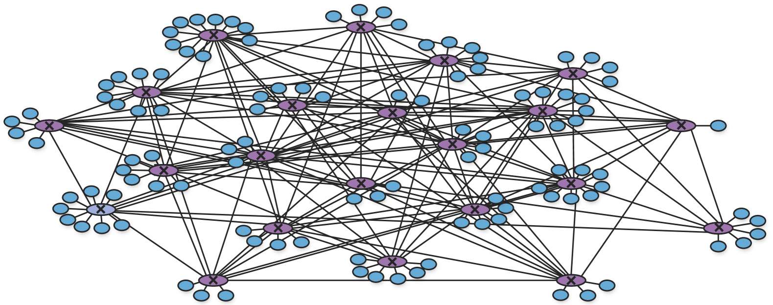
Figure 5: An example of an Erdős-Rényi (ER) network with 22 switches, 110 end-systems, and a link connection probability of 0.6.

V-A2 Comparison with the State-of-the-Art

To verify the high utilization, we compare our method with the state-of-the-art, namely MDM-len and MDM-rem[20], which are the online admission control methods in TSN/CBS architecture. These methods ensure real-time requirements by setting fixed delay budgets on queues and employing DCLC routing at runtime, with MDM-len using a cost function based on path length and MDM-rem relying on the remaining link rate. The evaluations compare the number of admitted flows across experiment cases varying in link connection probabilities, topology scales, requested flows, and AVB class number. Fig. 6(a)-(d) show the comparative results. Fig. 6(a) shows the results for different link connection probabilities $p$. Our method exhibits greater improvement over the MDM method when the link connection probability $p$ is smaller. This is because, at a smaller link connection probability $p$, the availability of network resources is lower. Our method can better overcome these limitations compared to fixed delay budgets by adaptively assigning and adjusting local deadlines, thus effectively increasing the flow admission capacity. Fig. 6(b) indicates that as the topology scale expands, the number of admitted flows increases for all methods. This growth is due to expanding available network resources with increased physical links. Fig. 6(c) shows that as the number of requested flows increases, the admission ratio, which represents the percentage of admitted flows to requested flows, decreases for all methods due to the limited available network resources. Fig. 6(d) illustrates that as the number of AVB classes increases, the number of admitted flows first increases and then decreases. This trend suggests that assigning too many or too few classes might not be optimal, making class assignments an interesting topic for future discussion. In summary, across the discussed cases, our method shows an average improvement of 59.4% over the MDM-len method and 95.2% over the MDM-rem method in terms of admitted flows.

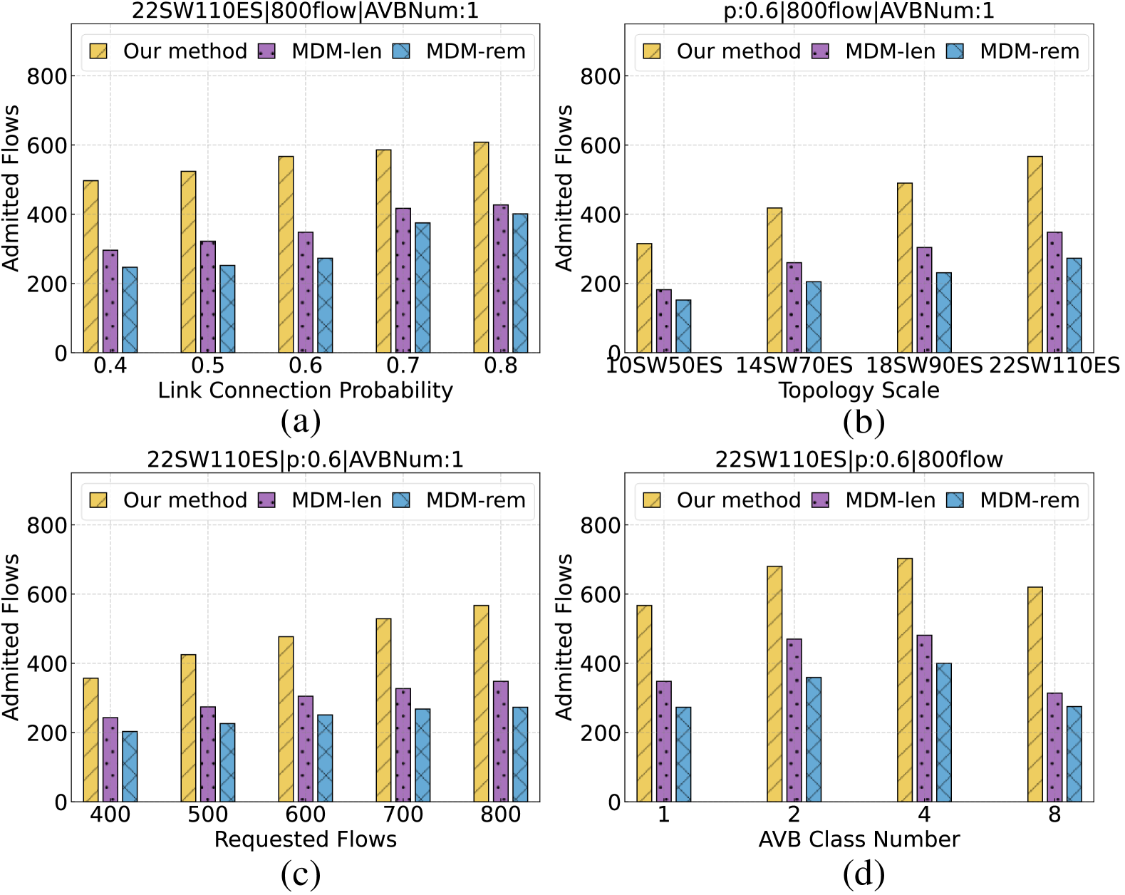
Figure 6: Comparison of our method with the state-of-the-art in terms of admitted flows.

V-A3 Comparison of Local Deadline Adjustment Strategies

To validate the effectiveness of our local deadline adjustment strategy proposed in Section 4, we compare it with three baseline strategies from [29]: equal partition (EP), load-based partition (LP), and available bandwidth-based Partition (ABP). The coefficients $\kappa^{(u,v)}$ for $(u,v)\in r_{f^{+}}$ in these strategies are listed in Table II. For the comparison, we adopt the adjusted local deadline $\hat{D}^{(u,v)}_{i}=D^{(u,v)}_{i}-(\sum_{(u^{\prime},v^{\prime})\in r_{f^{+}}}D^{(u^{\prime},v^{\prime})}_{i}-D_{f^{+}}^{\rm E2E})\cdot\kappa^{(u,v)}$ for the baseline strategies in place of the output from Algorithm 1, while the other parts follow the online admission control framework outlined in Section III. The evaluations compare the number of admitted flows across experiment cases, which are consistent with those used in Section V-A2. Fig. 7(a)-(d) displays the experimental results, indicating that our strategy achieves an average increase in the number of admitted flows by 40.0%, 32.0%, and 34.7% compared to the EP, LP, and ABP strategies, respectively. The EP strategy leads to the lowest number of admitted flows because it uniformly reduces local deadlines to meet the new flow deadline without considering the specific characteristics of the existing network configuration. The LP and ABP outperform EP because they indirectly incorporate residual bandwidth balancing into their strategies by utilizing the proportions of traffic load and available residual bandwidth, respectively. Our strategy outperforms others because it iteratively finds an adjustment that ensures the extra bandwidths are allocated according to the proportion of available residual bandwidths between egress ports. This approach directly balances the residual bandwidth across egress ports, preventing some egress ports from becoming bottlenecks too early due to resource exhaustion.

TABLE II: Coefficients of Baseline Strategies

Strategy	EP	LP	ABP
${{\kappa^{(u,v)}}}^{1}$	${\frac{1}{|r_{f^{+}}|}}^{2}$	${\frac{\sum_{(u^{\prime},v^{\prime})\in r_{f^{+}}}B^{(u^{\prime},v^{\prime})}-B^{(u,v)}}{\left(|r_{f^{+}}|-1\right)\sum_{(u^{\prime},v^{\prime})\in r_{f^{+}}}B^{(u^{\prime},v^{\prime})}}}^{3}$	${\frac{R^{(u,v)}}{\sum_{(u^{\prime},v^{\prime})\in r_{f^{+}}}R^{(u^{\prime},v^{\prime})}}}^{4}$

• $\kappa^{(u,v)}$ denotes the proportion of the reduction in initial local deadline at egress port $(u,v)$ relative to the entire route $r_{f^{+}}$

• $|r_{f^{+}}|$ denotes the length of route $r_{f^{+}}$.

• $B^{(u,v)}=\sum_{f\in(\mathcal{F}\cup\{f^{+}\})^{(u,v)}}\rho_{f}$ denotes the load at egress port $(u,v)$.

• $R^{(u,v)}$ denotes the residual bandwidth at egress port $(u,v)$ as Eq. (11).

Figure 7: Comparison of our local deadline adjustment strategy in Section 4 with the baseline strategies in terms of admitted flows.

V-A4 Execution Time

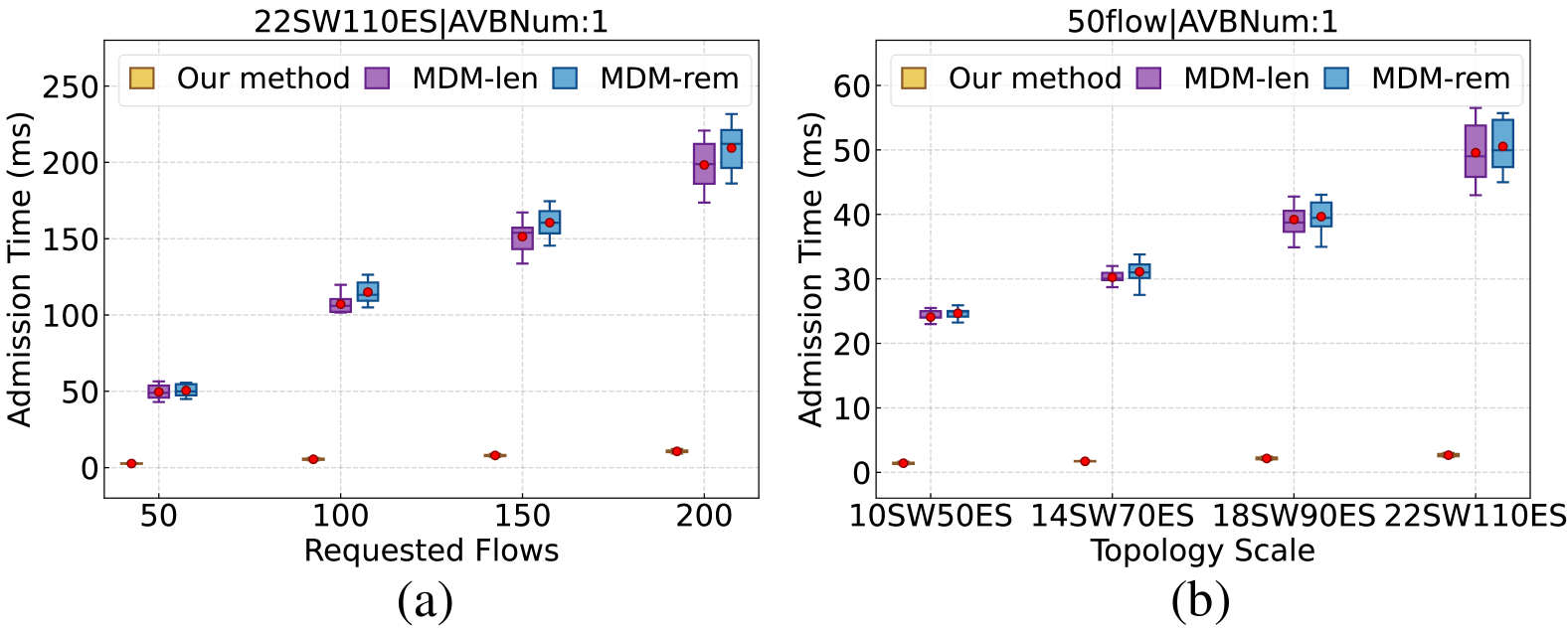
Figure 8: Comparison of our method with the state-of-the-art in terms of admission time.

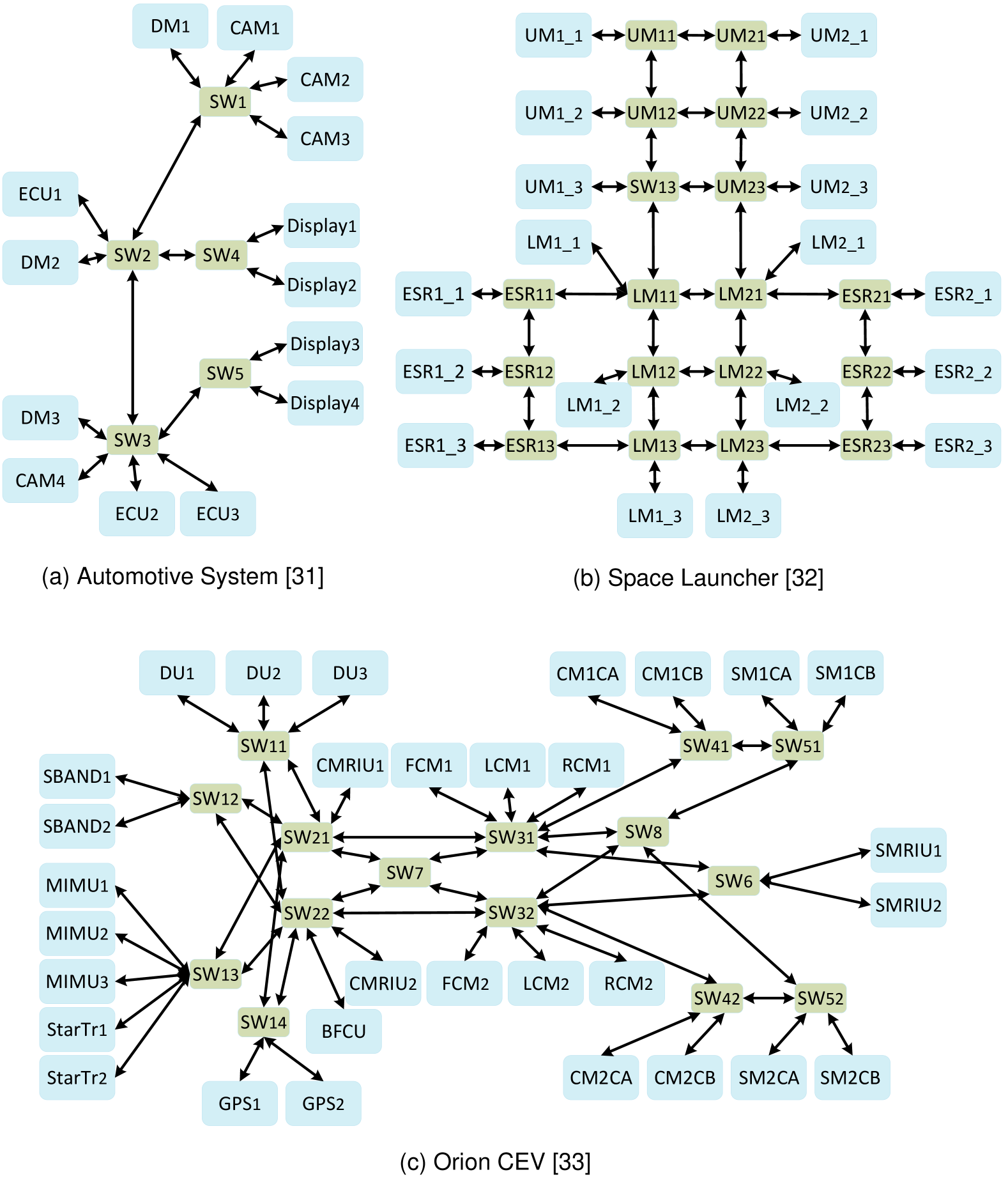
Figure 9: Topologies of three realistic test cases.

To confirm the efficiency and scalability, we compare our method with the state-of-the-art MDM-len and MDM-rem[20]. The evaluations focus on the admission time across experimental cases with varying requested flows and topology sizes. Fig. 8(a)-(b) demonstrate the experimental results using box plots, where each box corresponds to 10 cases and the red marker represents the mean value. Fig. 8(a) illustrates that the admission time for each method increases linearly with the number of requested flows. Specifically, for our method, the average admission times for admitting 50, 100, 150, and 200 flows are 2.7ms, 5.4ms, 8.0ms, and 10.6ms, respectively. Compared to the MDM methods, our method exhibits a markedly slower growth rate, indicating a significant decrease in the per-flow admission time. Fig. 8(b) displays the admission time for three methods across various topology scales. For our method, the average admission times for admitting 50 flows are 1.4ms, 1.7ms, 2.2ms, and 2.7ms, respectively. Compared to the MDM methods, our method demonstrates a smaller rise in admission time as the topology scale grows. In summary, for the presented cases, our method achieves an average reduction in admission time of 94.5% and 94.7% when compared to the MDM-len and MDM-rem methods, respectively. The per-flow admission time for large-scale scenarios involving 22SW110ES achieves less than 100$\mu$s. Our method significantly reduces admission time primarily for two reasons: Firstly, we shift the complexity of online routing to the offline phase. Secondly, our TSN/ATS+CBS architecture does not require calculating and shaping the arrival curve for preceding links. These improvements significantly reduce the admission time.

V-B Realistic Test Cases

TABLE III: Overview of Network Configuration Characteristics

Case	Nodes	Switches	Links	Link Speeds
Automotive System [31]	14	5	18	1Gbit/s (DM3$\leftrightarrow$ SW3) 100Mbit/s(others)
Space Launcher [32]	18	18	24	100Mbit/s
Orion CEV [33]	31	15	55	1Gbit/s

V-B1 Comparison in Realistic Test Cases

TABLE IV: Flows in the Automotive System Case

Class	Size (B)	Period (us)	Deadline (us)	Src	Dst	Proportion
A	256-1024	10000	10000	ECU	DM	40.8%
B	128or256	10000	10000	CAM	DM	29.6%
C	1446	1100	30000	CAM1	DM1	3.7%
	1446	1100	30000	CAM2	DM1	3.7%
	1446	1100	30000	CAM3	DM2	3.7%
	1446	1100	30000	CAM4	DM2	3.7%
	1446	1100	30000	CAM4	Display1	3.7%
	1446	1100	30000	CAM4	Display2	3.7%
D	1446	1100	30000	CAM4	DM3	7.4%

TABLE V: Flows in the Space Launcher Case

Class	Size(B)	Period(us)	Deadline(us)	Proportion
A	256-1024	10000	10000	21%
B	128or256	10000	10000	78%
C	1446	1100	30000	1%

TABLE VI: Flows in the Orion CEV Case

Class	Size(B)	Period (us)	Deadline (us)	Proportion
A	64-1518	4000	6800-7300	6%
	64-1518	8000	8700-15000	14%
	64-1518	16000	16000-30000	9%
B	64-1518	16000	17000-32000	13%
	64-1518	32000	34000-62000	14%
	64-1518	64000	67000-68000	2%
C	64-1518	64000	70000-130000	24%
	64-1518	128000	170000-190000	3%
D	64-1518	128000	170000-370000	15%

TABLE VII: Comparison in Three Realistic Test Cases

Case	Metric	Our Method	MDM-len	MDM-rem	EP	LP	ABP
Automotive System [31]	Admission Capacity1	217 (+28%)4	170 (0%)	170 (0%)	170 (0%)	194 (+14%)	126 (-26%)
	First Rejection2	48 (+2%)	47 (0%)	47 (0%)	48 (+2%)	48 (+2%)	6 (-87%)
	Per-Flow Admission Time3	13.3$\mu s$ (-90%)	137.7$\mu s$ (0%)	90.4$\mu s$ (-34%)	11.1$\mu s$ (-92%)	9.67$\mu s$ (-93%)	11.1$\mu s$ (-92%)
Space Launcher [32]	Admission Capacity	701 (+70%)	412 (0%)	418 (+1%)	557 (+35%)	540 (+31%)	383 (-7%)
	First Rejection	218 (+37%)	159 (0%)	121 (-24%)	9 (-94%)	9 (-94%)	9 (-94%)
	Per-Flow Admission Time	70.0 $\mu s$ (-88%)	565.4$\mu s$ (0%)	581.6$\mu s$ (+2%)	30.1$\mu s$ (-95%)	56.7$\mu s$ (-90%)	69.5$\mu s$ (-88%)
Orion CEV [33]	Admission Capacity	5653 (+18%)	4789 (0%)	4293 (-10%)	2000 (-58%)	2126 (-56%)	1969 (-59%)
	First Rejection	3588 (+75%)	2047 (0%)	1449 (-29%)	21 (-99%)	21 (-99%)	21 (-99%)
	Per-Flow Admission Time	78.3$\mu s$ (-79%)	370.1$\mu s$ (0%)	420.2$\mu s$ (+14%)	24.5$\mu s$ (-93%)	25.7$\mu s$ (-93%)	32.2$\mu s$ (-91%)

• Admission capacity is evaluated using a request flow set of 10000 flows, representing a large number of admission requests.

• First rejection refers to the index of the first flow rejected during the admission process.

• Per-flow admission time is measured using a request flow set of 100 flows, representing a high admission rate, which helps avoid underestimated results caused by frequent rejections.

• The baseline for comparison is the state-of-the-art MDM-len method.

We compare different methods across three realistic test cases. The methods consist of our method, MDM-len and MDM-rem (described in Section V-A2), and EP, LP, and ABP (described in Section V-A3). The three realistic test cases are the Automotive System [31], Space Launcher [32], and Orion CEV [33]. Their topologies and network configuration characteristics are presented in Fig. 9 and Table III. The attributes of the flow sets used for admission control are listed in Tables IV, V, and VI, which are derived from real-world cases. The comparison metrics include admission capacity, first rejection, and per-flow admission time. Admission capacity refers to the number of flows successfully admitted when processing a large set of request flows, reflecting the maximum admission capacity of the method. The first rejection indicates the index of the first flow rejected during the admission process, with a higher value suggesting that the method can better adapt to varying traffic requirements. Per-flow admission time refers to the average computation time required to admit each flow, reflecting the responsiveness to admission requests. The comparison results are summarized in Table VII.

First, our method is compared with MDM-len and MDM-rem methods. In terms of admission capacity, our method shows improvements across all three test cases, with a remarkable increase of 70% observed in the Space Launcher case. For the first rejection, our method also demonstrates improvement, with performance increasing by up to 75% in the Orion CEV case. Regarding per-flow admission time, our method reduces the time by over 79% compared to MDM-len. Additionally, even in large-scale scenarios, the per-flow admission time of our method is less than 100 $\mu s$. These results indicate that, with ATS support, our method dynamically adjusts local deadlines to balance residual bandwidth, thereby optimizing resource utilization and enhancing adaptability. Furthermore, our method avoids online routing and the calculation and shaping of arrival curves for preceding links, significantly reducing admission time.

Next, our method is compared with EP, LP, and ABP, which use different local deadline adjustment strategies. For admission capacity, our method shows an increase in the number of admitted flows across all three test cases, with an improvement of over 165% in the Orion CEV case. In terms of first rejection, our method performs similarly to the EP and LP methods in the Automotive System case, but shows significant improvements in the large-scale scenarios of Space Launcher and Orion CEV. In the Space Launcher case, the first rejection for EP, LP, and ABP occurs at the 9th flow, while our method postpones it until the 218th flow. In the Orion CEV case, the first rejection for EP, LP, and ABP happens at the 21st flow, while our method postpones it until the 3588th flow. Regarding per-flow admission time, our method shows an increase compared to EP, LP, and ABP, but the admission times remain within the same order of magnitude (e.g., tens of microseconds). In summary, compared to the EP, LP, and ABP methods that directly adjust local deadlines, our method adjusts local deadlines by balancing the remaining bandwidth. Although this introduces some additional admission time overhead, it significantly improves admission capacity and postpones the occurrence of the first rejection. Particularly in large-scale scenarios, our method significantly increases the number of consecutive admissions, demonstrating enhanced adaptability.

V-B2 In-Depth Comparison in the Orion CEV Case

We conduct an in-depth comparison of different methods in the Orion CEV case, focusing on the distribution of successful admitted flows and bottleneck egress port counts during the admission process. The experiment uses a request flow set comprising 6000 flows, which are divided into 120 flow groups, each containing 50 flows. For each flow group, two metrics are recorded when the admission decision for the last flow in the group is completed: the number of successful admitted flows within the group and the number of bottleneck egress ports in the network. A bottleneck egress port is defined as an egress port where the available residual bandwidth is less than 10% of $idSl_{\max}$, where $idSl_{\max}$ is the upper bandwidth limit allocated to all AVB classes at the egress port. The comparison results are shown in Fig. 10, where each subplot corresponds to a different method. In each subplot, the x-axis represents the index of the flow groups requesting admission. The blue points indicate the number of successful admitted flows in the corresponding flow group (ranging from 0 to 50), and the red points represent the number of bottleneck egress ports.

From the comparison results in Fig. 10, it is observed that our method postpones the appearance of bottleneck egress ports until the 65th flow group. In comparison, MDM-len reaches this point in the 26th group, MDM-rem in the 24th group, EP in the 13th group, LP in the 9th group, and ABP in the 8th group. Further observation of the admitted flows reveals that, after the appearance of bottleneck egress ports, our method, MDM-len, and MDM-rem begin to fail to admit all 50 flows as the egress ports gradually become unavailable. Additionally, as the number of bottleneck egress ports increases, the admission ratio within each flow group decreases. Overall, our method enhances admission capacity and delays the first rejection by effectively postponing the occurrence of bottleneck egress ports. The EP, LP, and ABP methods are unable to admit all 50 flows even before bottleneck egress ports appear. This is because the local deadlines determined by their direct deadline adjustment strategies cannot be guaranteed within the available residual bandwidth, leading to the rejection of some flows. In contrast, our method avoids this issue by using a local deadline adjustment strategy that balances the residual bandwidth, thereby postponing the first rejection and achieving higher admission capacity.

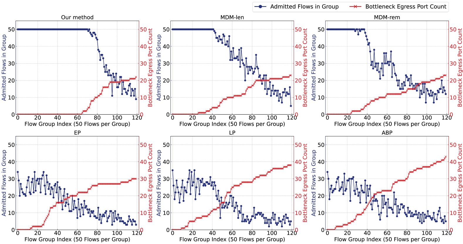
Figure 10: Comparison of distribution in successful admission flows and bottleneck egress port count in Orion CEV case.

VI Conclusion

In this work, we propose a fast and high-utilization online admission control method that ensures real-time requirements for time-critical ET traffic. The experimental results from synthetic test cases show that, compared to the state-of-the-art, our method increases the number of admitted flows by an average of 59% and saves the admission time by an average of 95%. Evaluations across three realistic test cases reveal that our method postpones the occurrence of bottleneck egress ports and the first rejection during the admission process, thereby enhancing adaptability. In the future, we will explore dynamically adjusting local deadlines beyond the route to mitigate flow rejection caused by resource-exhausted bottlenecks.

References

- [1] Stream Reservation Protocol (SRP) Enhancements and Performance Improvements, IEEE Std. 802.1Qcc, 2018. [Online]. Available: https://1.ieee802.org/tsn/802-1qcc/.
- [2] Enhancements for Scheduled Traffic, IEEE Std. 802.1Qbv, 2016. [Online]. Available: http://www.ieee802.org/1/pages/802.1bv.html.
- [3] Cyclic Queuing and Forwarding, IEEE Std. 802.1Qch, 2015. [Online]. Available: https://1.ieee802.org/tsn/802-1qch/.
- [4] N. G. Nayak, F. Durr, and K. Rothermel, “Incremental Flow Scheduling and Routing in Time-Sensitive Software-Defined Networks,” IEEE Trans. Ind. Inf., vol. 14, no. 5, pp. 2066–2075, May 2018.
- [5] A. Alnajim, S. Salehi, and C.-C. Shen, “Incremental Path-Selection and Scheduling for Time-Sensitive Networks,” in Proc. Glob. Commun. Conf., Dec. 2019, pp. 1–6.
- [6] Y. Huang, S. Wang, T. Huang, B. Wu, Y. Wu, and Y. Liu, “Online Routing and Scheduling for Time-Sensitive Networks,” in Proc. 41st Int. Conf. Distrib. Comput. Syst., Jul. 2021, pp. 272–281.
- [7] Z. Feng, Z. Gu, H. Yu, Q. Deng, and L. Niu, “Online Rerouting and Rescheduling of Time-Triggered Flows for Fault Tolerance in Time-Sensitive Networking,” IEEE Trans. Comput.-Aided Des. Integr. Circuits Syst., vol. 41, no. 11, pp. 4253–4264, Nov. 2022.
- [8] C. Gärtner, A. Rizk, B. Koldehofe, R. Guillaume, R. Kundel, and R. Steinmetz, “Fast incremental reconfiguration of dynamic time-sensitive networks at runtime,” Comput. Netw., vol. 224, p. 109606, Apr. 2023.
- [9] Y. Huang, S. Wang, X. Zhang, T. Huang, and Y. Liu, “Flexible Cyclic Queuing and Forwarding for Time-Sensitive Software-Defined Networks,” IEEE Trans. Netw. Serv. Manage., vol. 20, no. 1, pp. 533–546, Mar. 2023.
- [10] K. Cao and F. Yang, “PRIS: Online Routing and Scheduling Making CQF Flexible in Dynamic Time-Sensitive Networks,” in Proc. 9th Int. Conf. Comput. Commun., 2023, pp. 22–28.
- [11] IEEE Standard for Local and Metropolitan Area Networks - Bridges and Bridged Networks, IEEE Std. 802.1Q, 2018. [Online]. Available: https://standards.ieee.org/ieee/802.1Q/6844/.
- [12] Forwarding and Queuing Enhancements for Time-Sensitive Streams, IEEE Std. 802.1Qav, 2009. [Online]. Available: https://www.ieee802.org/1/pages/802.1av.html.
- [13] IEEE Standard for Local and Metropolitan Area Networks - Bridges and Bridged Networks Amendment: Asynchronous Traffic Shaping, IEEE Std. 802.1Qcr, 2018. [Online]. Available: https://1.ieee802.org/tsn/802-1qcr/.
- [14] J. A. R. De Azua and M. Boyer, “Complete modelling of AVB in Network Calculus Framework,” in Proc. 22nd Int. Conf. Real-Time Netw. Syst., 2014, pp. 55–64.
- [15] M. Ashjaei, G. Patti, M. Behnam, T. Nolte, G. Alderisi, and L. Lo Bello, “Schedulability analysis of Ethernet Audio Video Bridging networks with scheduled traffic support,” Real-Time Syst, vol. 53, no. 4, pp. 526–577, Jul. 2017.
- [16] L. Zhao, P. Pop, Z. Zheng, H. Daigmorte, and M. Boyer, “Latency Analysis of Multiple Classes of AVB Traffic in TSN With Standard Credit Behavior Using Network Calculus,” IEEE Trans. Ind. Electron., vol. 68, no. 10, pp. 10 291–10 302, Oct. 2021.
- [17] N. Reusch, L. Zhao, S. S. Craciunas, and P. Pop, “Window-Based Schedule Synthesis for Industrial IEEE 802.1Qbv TSN Networks,” in Proc. 16th IEEE Int. Conf. Factory Commun. Syst., Apr. 2020, pp. 1–4.
- [18] L. Zhao, X. Zhang, H. Feng, and Z. Li, “Incremental Performance Analysis for Accelerating Verification of TSN Network Reconfigurations,” IEEE Trans. Netw. Serv. Manage., pp. 1–16, 2024.
- [19] J. W. Guck, M. Reisslein, and W. Kellerer, “Function Split Between Delay-Constrained Routing and Resource Allocation for Centrally Managed QoS in Industrial Networks,” IEEE Trans. Ind. Inf., vol. 12, no. 6, pp. 2050–2061, Dec. 2016.
- [20] L. Maile, K.-S. J. Hielscher, and R. German, “Delay-Guaranteeing Admission Control for Time-Sensitive Networking Using the Credit-Based Shaper,” IEEE Open J. Commun. Soc., vol. 3, pp. 1834–1852, Oct. 2022.
- [21] L. Zhao, Y. Yan, and X. Zhou, “Minimum Bandwidth Reservation for CBS in TSN With Real-Time QoS Guarantees,” IEEE Trans. Ind. Inf., vol. 20, no. 4, pp. 6187–6198, Apr. 2024.
- [22] J. Specht and S. Samii, “Urgency-Based Scheduler for Time-Sensitive Switched Ethernet Networks,” in Proc. 28th Euromicro Conf. Real-Time Syst., Jul. 2016, p. 11.
- [23] E. Mohammadpour, E. Stai, M. Mohiuddin, and J.-Y. Le Boudec, “Latency and Backlog Bounds in Time-Sensitive Networking with Credit Based Shapers and Asynchronous Traffic Shaping,” in Proc. 30th Int. Teletraffic Congr., Sep. 2018, pp. 1–6.
- [24] J.-Y. Le Boudec and P. Thiran, Network Calculus: A Theory of Deterministic Queuing Systems for the Internet, ser. Springer-Verlag Lecture Notes on Computer Science. New York: Springer, 2001, no. 2050.
- [25] J.-Y. Le Boudec, “A Theory of Traffic Regulators for Deterministic Networks With Application to Interleaved Regulators,” IEEE/ACM Trans. Networking, vol. 26, no. 6, pp. 2721–2733, Dec. 2018.
- [26] L. Zhao, P. Pop, and S. Steinhorst, “Quantitative Performance Comparison of Various Traffic Shapers in Time-Sensitive Networking,” IEEE Trans. Netw. Serv. Manage., vol. 19, no. 3, pp. 2899–2928, Sep. 2022.
- [27] R. Enns, M. Bjorklund, J. Schoenwaelder et al., “Network configuration protocol (netconf),” Internet Engineering Task Force, RFC 6241, 2011. [Online]. Available: https://tools.ietf.org/html/rfc6241
- [28] J. Y. Yen, “Finding the K Shortest Loopless Paths in a Network,” Management Science, vol. 17, no. 11, pp. 712–716, 1971.
- [29] A. Sahoo, Z. Wei, and J. Weijia, “Partition-based admission control in heterogeneous networks for hard real-time connections,” in Proc. 10th Int. Conf. Parallel. Distrib. Comput., 1997.
- [30] A. A. Hagberg, D. A. Schult, and P. J. Swart, “Exploring network structure, dynamics, and function using NetworkX,” in Proc. Python Sci. Conf., 2008.
- [31] J. Migge, J. Villanueva, N. Navet, and M. Boyer, “Insights on the Performance and Configuration of AVB and TSN in Automotive Ethernet Networks,” in Proc. 9th Eur. Congr. Embed. Real Time Softw. Syst., 2018.
- [32] P. Keller and N. Navet, “Approximating WCRT through the aggregation of short simulations with different initial conditions: Application to TSN,” in Proc. 30th Int. Conf. on Real-Time Netw. and Syst., 2022.
- [33] D. Tamas–Selicean, “Design of Mixed-Criticality Applications on Distributed Real-Time Systems,” Ph.D. dissertation, Dept. Appl. Math. and Comp. Sci., Technical Univ. of Denmark, Kongens Lyngby, DK, 2014.