Differentiable Folding for Nearest Neighbor Model Optimization

Abstract

The Nearest Neighbor model is the de facto thermodynamic model of RNA secondary structure formation and is a cornerstone of RNA structure prediction and sequence design. The current functional form (Turner 2004) contains $\approx 13,000$ underlying thermodynamic parameters, and fitting these to both experimental and structural data is computationally challenging. Here, we leverage recent advances in differentiable folding, a method for directly computing gradients of the RNA folding algorithms, to devise an efficient, scalable, and flexible means of parameter optimization that uses known RNA structures and thermodynamic experiments. Our method yields a significantly improved parameter set that outperforms existing baselines on all metrics, including an increase in the average predicted probability of ground-truth sequence-structure pairs for a single RNA family by over 23 orders of magnitude. Our framework provides a path towards drastically improved RNA models, enabling the flexible incorporation of new experimental data, definition of novel loss terms, large training sets, and even treatment as a module in larger deep learning pipelines. We make available a new database, RNAometer, with experimentally-determined stabilities for small RNA model systems.

1 Introduction

The Nearest Neighbor model (NN model), a.k.a. the Turner rules, is the gold standard thermodynamic model of RNA secondary structure formation. The model assigns a free energy by decomposing a seqeunce-structure pair into a non-overlapping set of “loops” and ascribing a free energy change to each loop. This is amenable to dynamic programming, enabling the efficient calculation of the partition function [1]. The model and corresponding suite of algorithms undergird popular software packages such as mfold [2], NUPACK [3], ViennaRNA [4], and RNAstructure [5].

The NN model consists of $\approx 13,000$ thermodynamic parameters [6]. The standard fitting procedure involves linearly interpolating $\approx 300$ parameters to experimentally measured free energy changes [7, 8]. The complete parameter set is then extrapolated from this set of base parameters. This procedure is complicated; though tractable, it is challenging to reproduce, requires substantial domain expertise, cannot include known sequence-structure data, and is a noisy fit given the loss in information by assuming linear dependencies.

Prior methods attempt to improve RNA structure prediction, either with advanced NN parameter fitting schemes or via alternative modeling techniques. In Ref. [9], the authors developed two approaches to optimize parameters for the NN model. The first was gradient descent to optimize the “Boltzmann Likelihood” of known RNA structures. This is similar to prior probabilistic methods like CONTRAfold [10], but incorporates thermodynamic constraints into the optimization. This method proved too slow to optimize parameters. Instead, an iterative constrained optimization heuristic was deployed. A key feature of Ref. [9] is that the parameters are fit both to known thermodynamic experiments and to a data set of known RNA structures. This helps to prevent over-fitting and ensures the parameters are interpretable. Alternative modeling techniques include (i) deep learning and (ii) generative probabilistic models via stochastic context free grammars (SCFGs), which learn the parameters of the model rather than replacing the model. Deep learning methods have generally struggled to generalize outside their training data [11, 12], a property clear in the RNA results for CASP15 [13] and CASP16. SCFGs similarly suffer from over-fitting [14] but can achieve robust performance with careful validation [15, 16].

This work is an evolution of Ref. [9] in which we demonstrate how differentiable folding can be adapted for efficient, flexible, and transparent NN parameter fitting. Differentiable folding is a recently developed method for RNA design in which gradients of McCaskill’s recursions [1] for computing the RNA partition function can be directly computed via automatic differentiation. Here, rather than optimizing a sequence distribution with respect to a fixed model of RNA thermodynamics, we optimize the parameters of the underlying thermodynamic model using ground truth structural and thermodynamic information defined for fixed input sequences. The flexibility of our method also lets us incorporate thermodynamic data, like Ref. [9], but also to use even more complex loss functions. In essence, any continuous and differentiable loss function can be optimized. Our method is fast enough to enable us to probe various objective functions and to do extensive cross validation.

As a demonstration, we fit parameters to minimize diverse objective functions. First, we define individual objective functions over different data sources (i.e. structural and thermodynamic). Given the flexibility in the choice of objective function, we can (i) control over-fitting to individual RNA families and (ii) evaluate the trade-offs imposed by each data source by performing optimizations with varying relative weights assigned to each objective. We also explore the role of parameter inter-dependencies by performing optimizations using both the highly constrained rules of Ref. [8] as well as a minimal set of symmetries across parameters. Lastly, we perform optimizations with respect to different versions of the recursions varying in their treatment of coaxial stacks, terminal mismatches, and dangling ends, the subject of previous work [17, 18].

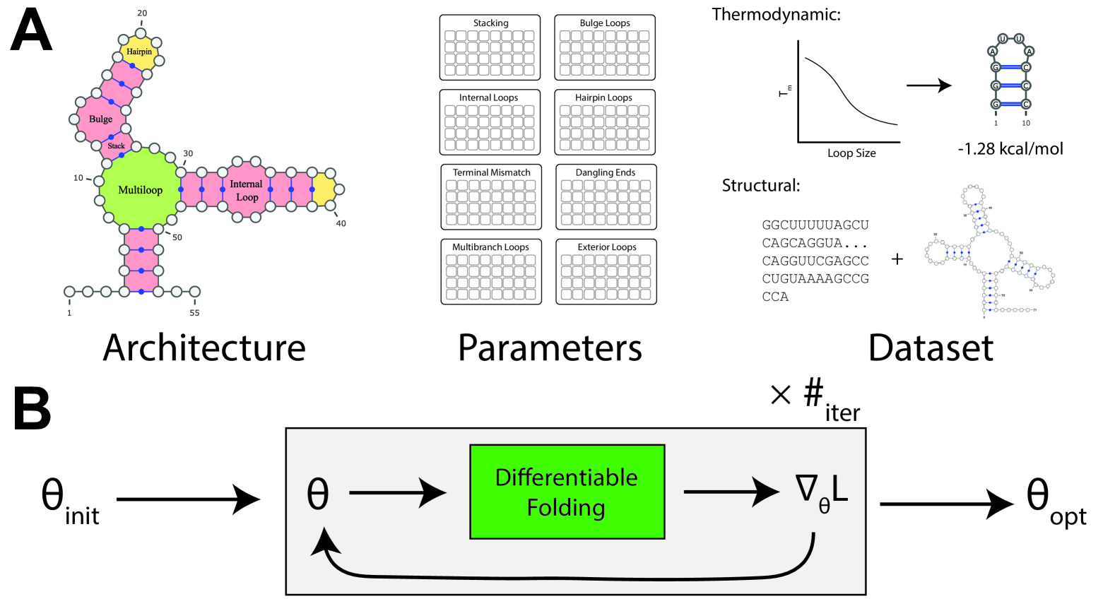
Figure 1: An overview of our method for NN Model parameter optimization. A. NN model parameter fitting can be formulated as an optimization problem akin to training a neural network. The architecture is defined by the RNA folding grammar, the free parameters are (a subset of) the corresponding thermodynamic values, and the dataset comprises of (i) experimental optical melting experiments, which ascribe free energies to sequence-structure pairs, and (ii) structural data comprising of sequences and their most likely structures. B. Our method for parameter optimization via differentiable folding, in which a loss function is defined over thermodynamic quantities and its gradient is computed via differentiable folding for gradient descent.

Our method yields drastically improved NN parameters for both structure prediction and agreement with thermodynamic experiments. This is despite strict family-fold validation to prevent over-fitting. Our optimized parameters will be available in the next version of RNAstructure.

2 Methods

Here we describe our general framework for optimizing nearest neighbor parameters via differentiable folding, as well as the specific objective functions used in this work.

2.1 General Purpose Framework

In Ref. [19], a generalization of McCaskill’s algorithm is given that is well-defined over a continuous (i.e. probabilistic) sequence representation. When implemented in an automatic differentiation framework, gradients of the partition function can be computed with respect to the sequence for inverse folding. This paradigm is known as differentiable folding. Crucially, RNA design requires a fixed parameterization of the NN model. Formally, the partition function $Z_{q,\theta}$ is parameterized by two independent parameter sets: the (continuous or discrete) sequence $q$, and the NN parameters $\theta$. Matthies et al. originally developed differentiable folding to enable the automatic calculation of $\nabla_{q}Z_{q,\theta}$ where $q$ is represented as a continuous variable. Note that we explicitly refer to the partition function as the primary thermodynamic quantity of interest, but in practice differentiable folding can be applied to secondary thermodynamic quantities of interest, e.g. the free energy and probability of a sequence-structure pair.

Figure 2: Optimizing Nearest Neighbor parameters via gradient descent under our default settings (i.e. $\alpha=0.5$, no terminal mismatches, dangling ends, or coaxial stacks (equivalent to d0 in ViennaRNA), and the extrapolation rules of Ref. [8]). A. The change in the average log-probability for all sequences of length $n\leq 512$ for each family within the ArchiveII dataset. Since optimization is performed via stochastic gradient descent, points depict periodic evaluations of the entire dataset. 23S ribosomal RNAs are excluded from the training set. Dashed lines depict baseline values computed via ViennaRNA with the default Turner 2004 parameters. B. The change in normalized mean squared error (MSE) between the ground truth free energy values from the thermodynamic dataset of optical melting experiments and the computed values. Dashed lines depict this value evaluated using ViennaRNA with the Turner 2004 parameters under d0.

In this work, we adapt differentiable folding for an entirely different optimization problem: fitting the underlying NN parameters $\theta$. Given ground-truth structural and thermodynamic data, we can define an arbitrary (continuous and differentiable) objective function $O(\theta)$ expressing the degree to which a model parameterized by $\theta$ fits the data. We can directly compute $\nabla_{\theta}O(\theta)$ via differentiable folding and update $\theta$ via gradient descent. This application of differentiable folding naturally scales to longer sequences than for RNA design as the RNA sequences are discrete rather than continuous, omitting the need to differentiate the memory-intensive recursions defined in Ref. [19]. In addition, our implementation is in JAX and can therefore compile to a range of targets (e.g. CPU, GPU, and TPU), rendering our method extremely efficient compared to existing work. All optimizations were performed on a single NVIDIA 80 GB A100 GPU in less than 2 days.

2.2 Objective Functions and Optimization Details

We consider two types of data: thermodynamic and structural. Thermodynamic data consist of sequence-structure pairs with known free energy changes determined via optical melting experiments. These thermodynamic data serve as the basis for standard NN parameter fitting schemes. Formally, we have a library of optical melting data $M$ with $(q,s,\Delta G,\sigma^{2})\in M$ where $q$ is an RNA sequence, $s$ is a valid secondary structure for $q$, $\Delta G$ is the experimentally-derived free energy change for $q$ folding into $s$, and $\sigma^{2}$ is the variance of $\Delta G$. Define the thermodynamic loss $\mathcal{L}_{\text{thermo}}$ of a given model parameterization $\theta$ as

$$\mathcal{L}_{\text{thermo}}(\theta)=\frac{1}{|M|}\sum_{(q,s,\Delta G,\sigma^{2})\in M}\frac{(\Delta G-F_{\theta}(q,s))^{2}}{\sigma^{2}}$$ (1)

where $F_{\theta}(q,s)$ is the computed free energy of the sequence structure pair $(q,s)$ given model parameters, $\theta$. We constructed $M$ by compiling $2,280$ optical melting experiments from $>100$ independent publications, which we filtered to $1,817$ experiments for optimization. We refer to this dataset as “RNAometer” (see Supplementary Information).

Structural data consist of sequence-structure pairs where secondary structures are determined by comparative sequence analysis. Formally, a library of structural data $S$ consists of pairs $(q,s^{*})\in S$ where $s^{*}$ is the known secondary structure for sequence $q$. In this work, we define $S$ as the ArchiveII dataset of $3,847$ RNA sequences with known secondary structures [20]. ArchiveII is a standard benchmark for secondary structure prediction accuracy [21, 12, 22] and contains sequences spanning RNA families, including 16S, 23S, and 5S ribosomal RNA, group I self-splicing introns, signal recognition particle RNA, RNase P, tRNA, tmRNA, and telomerase RNA. We preprocess all secondary structures by removing pseudoknots to leave the largest set of pseudoknot-free pairs via RemovePseudoknots in RNAstructure [23, 5].

Following recent work on fitness functions in RNA design algorithms [24], we design a structural objective function based on maximizing the probability of the structure in equilibrium,

$$p_{\theta}(s^{*}|q)=\frac{1}{Z_{q,\theta}}\exp(-\beta F_{\theta}(q,s^{*}))$$ (2)

where $\beta$ is the inverse of the product of temperature (set to $37\text{ C}^{\circ}$) and the Boltzmann constant. This is equivalent to the “Boltzmann Likelihood” method of Ref. [9] and is similar to how probabilistic models are often trained [15, 14, 10].

Care must be taken to prevent over-fitting an RNA secondary structure model to a subset of RNA families as (i) RNA families are not represented equally in structural databases and (ii) RNA families vary significantly in average sequence length and therefore in absolute scale of $p_{\theta}(s^{*}|q)$ [11, 14]. To mitigate over-fitting, we define our structural objective function as the average of expected log-probabilities across families,

$$\mathcal{L}_{\text{struct}}(\theta)=\frac{1}{|\mathcal{F}|}\sum_{f\in\mathcal{F}}\frac{1}{|S_{f}|}\sum_{(s^{*},q)\in S_{f}}\log\left(p_{\theta}\left(s^{*}|q\right)\right)$$ (3)

where $\mathcal{F}$ denotes the set of RNA families and $S_{f}\subseteq S$ is the subset of the structural dataset corresponding to family $f$. This is equivalent to the average logarithmic geometric mean across families, as the geometric mean is equivalent to the exponential of the arithmetic mean of logarithms. We chose this loss function because the geometric mean is robust to differences of scale between averaged quantities. In this way, the optimization will not be biased towards increasing the probability of shorter sequence-structure pairs (e.g. tRNA) compared to longer ones (e.g. 16S ribosomal RNA).

Given objective functions for each data source, we express a joint objective function

$$\mathcal{L}(\theta)=(1-\alpha)\mathcal{L}_{\text{struct}}(\theta)+\alpha\mathcal{L}_{\text{thermo}}(\theta)$$ (4)

where $0\leq\alpha\leq 1$ is a mixing factor which we introduce to control the relative importance of $\mathcal{L}_{\text{struct}}$ and $\mathcal{L}_{\text{thermo}}$. Crucially, we can compute $\nabla_{\theta}\mathcal{L}(\theta)$ automatically via differentiable folding.

In practice, one does not directly optimize $\theta$ but instead a base set of parameters $\theta_{\text{base}}$ that is deterministically extrapolated to $\theta$. This is both to preserve necessary symmetries between parameters and to mitigate over-fitting. We consider two distinct extrapolation schemes. First, we consider the simplest extrapolation that applies the minimal set of symmetries required to preserve thermodynamic interpretability (e.g. enforcing equal stacking parameters for stacking motifs that are identical up to $5^{\prime}\to 3^{\prime}$ and $3^{\prime}\to 5^{\prime}$ orientation). In total, there are $12,291$ values in $\theta_{\text{base}}$ when applying these symmetries (excluding coaxial stacks). Second, we consider a slightly modified version of the extrapolation rules introduced by Ref. [8] that map a set of $293$ base parameters to the full set of NN parameters. Our modified rule set considers a set of $284$ base parameters, which excludes coaxial stacking parameters.

The final detail of the optimization problem is the treatment of terminal mismatches, dangling ends, and coaxial stacks. These three accoutrements apply to multi-loops and exterior-loops. The first and simplest model we consider does not include any of these contributions. The second model we optimize allows a single nucleotide to contribute with all its possible favorable interactions, and is the default in ViennaRNA [4]. Following ViennaRNA naming conventions, we refer to these models as d0 and d2, respectively. We do not consider coaxial stacks in this work.

The direct calculation of $\nabla_{\theta}\mathcal{L}_{\text{struct}}(\theta)$ far exceeds the memory constraints of state-of-the-art GPUs given the large number of data points in the ArchiveII dataset. This constraint can be alleviated via gradient accumulation, by which gradients from multiple smaller mini-batches are collected before updating model weights, effectively simulating a larger batch size without increasing memory usage. Furthermore, we employ a form of stochastic gradient descent by which we randomly sample 32 sequence-structure pairs from each family to estimate the average intra-family log probability at each iteration. We also restrict the training set to sequences of length $n\leq 512$. This includes independent folding domains for 16S and 23S rRNA, which are included in ArchiveII as complete structures and as structures divided into domains [25]. We omit the 23S rRNA and group II intron families from the calculation of $\mathcal{L}_{\text{struct}}(\theta)$ as each family has fewer than 32 sequences with $n\leq 512$. This optimization yields an efficient calculation of $\nabla_{\theta}\mathcal{L}_{\text{struct}}(\theta)$, with each gradient update requiring $\sim 17.5$ minutes on a single NVIDIA A100 80 GB GPU. By default, we perform 150 iterations of gradient descent with an Adam optimizer and a learning rate of $\eta=0.1$.

	Thermodynamic Loss (Normalized MSE)		Structural Loss (average log-probability)
Parmeters	Single Stranded	Duplex	16S	5S	grp1	RNaseP	srp	telomerase	tmRNA	tRNA
Optimized	12.0	25.5	-46.6	-12.3	-44.1	-44.4	-24.5	-86.8	-43.8	-6.5
Family-Fold Val.	12.0	25.8	-48.0	-12.9	-44.9	-46.3	-25.0	-94.9	-46.0	-6.9
Optimized (no rules)	11.6	22.3	-44.4	-11.4	-42.3	-43.4	-23.4	-82.6	-42.2	-6.6
Family-Fold Val. (no rules)	11.5	22.4	-49.1	-13.0	-46.6	-47.6	-27.3	-95.5	-47.4	-7.1
Turner 2004	17.2	61.9	-69.3	-16.5	-73.4	-62.1	-34.3	-162.3	-72.6	-11.3
Andronescu 2007	25.5	104.0	-61.5	-17.6	-69.7	-60.4	-31.9	-147.8	-77.6	-9.6
Turner 1999	59.8	122.1	-65.0	-17.4	-73.4	-62.3	-34.5	-166.1	-78.1	-11.6

Table 1: Performance on thermodynamic and structural datasets with our optimized parameters vs. baselines for d0 recursions with $\alpha=0.5$. The structural loss is reported for all sequences of length $n\leq 512$ for each family within ArchiveII. All log-probabilities are reported in base $e$ (natural logarithm). Parameters labeled “Optimized” were trained on all families, with and without the extrapolation rules of Ref. [8]. For rows labeled “Family-Fold Validation,” structural losses represent the value obtained via optimization with the corresponding family excluded and thermodynamic losses represent the average value over all such optimizations (see Supplementary Information). “Turner 2004,” “Andronescu 2007,” and “Turner 1999” refer to the parameters from Ref. [7], Ref. [9], and Ref. [26], respectively. 16S and 5S refer to 16S and 5S ribosomal RNA, respectively. grp1 refers to group I introns.

3 Results

We first optimized the NN parameters under our default settings: no terminal mismatches, dangling ends, or coaxial stacks (ViennaRNA d0 in ), $\alpha=0.5$ (equal weight of structural and thermodynamic losses), and the extrapolation rules of Ref. [8] (to conservatively control over-fitting). We achieved substantially better performance on all objectives than any existing parameter set in ViennaRNA (Table 1, Figure 2). Optimized parameters improved the average probability of all sequence-structure pairs for 6 of 8 families in the training set by a factor of $1.9$ to $8.9\times 10^{23}$ (Table S2). Additionally, the normalized MSE between free energies obtained via optical melting experiments and computed values is $59.4\%$ and $74.7\%$ lower using our optimized parameters than using the default parameters in ViennaRNA for single-stranded and duplex RNAs, respectively. Note that the initial loss values in our optimization do not equal the baseline values as we initialize with the default parameters in RNAstructure rather than those in ViennaRNA.

We evaluate our parameters on all sequence-structure pairs with $n>512$ as well as on all 23S ribosomal RNA sequence-structure pairs with $n<512$, revealing an average improvement in probability by a factor of $7.9\times 10^{4}$ to $1.3\times 10^{53}$ across all unseen datasets (Table S6). For example, despite not including any group2-family sequences in our training set, our parameters improve the average probability by a factor of $2.8\times 10^{7}$. As an additional measure against over-fitting, we performed family-fold validation. Family-fold validation is a form of cross validation where each family is held out as the validation set [11]. We found that each family improves similarly when excluded from the training set (Table 1 and Supplementary Information).

Next, we performed optimizations with variants of the objective function and the recursions, i.e., the relative importance of structural and thermodynamic data, the method of extrapolation to a full set of NN parameters, and the treatment of terminal mismatches and dangling ends. We first repeated the optimization under our default settings but with a range of $\alpha$ values to explore the relative tradeoff between thermodynamic and structural loss terms. As expected, lower/higher values of $\alpha$ yield parameters with decreased/increased agreement with structural data and increased/decreased agreement with thermodynamic data (Figure S2A). This highlights the flexibility of our method in accommodating a desired trade-off between data sources.

We next repeated the default optimization using the extrapolation scheme that only applies the minimal set of symmetries to preserve thermodynamic interpretability, increasing $|\theta_{\text{base}}|$ (and therefore the degrees of freedom) from $284$ to $12,291$. As expected, the increased degrees of freedom yielded slightly improved performance but were not as robust to family-fold validation (see Table 1).

Lastly, we repeated the optimization for each choice of parameter extrapolation but with the more sophisticated treatment of terminal mismatches and dangling ends as per the d2 option in ViennaRNA. We achieve similar improvement as with d0, significantly outperforming all tested parameter sets in ViennaRNA on all objectives (see Table S1) and generalizing to the evaluation set (see Table S5). In general, our optimized d2 parameters slightly outperform their d0 counterparts, likely due to d2 being a more expressive grammar. For example, when extrapolating via the rules of Ref. [8], the optimized d2 parameters provide the most accurate structure predictions for 7 of 8 families (Tables S2 and S3) included in the training set and 6 of 7 unseen datasets (Tables S6 and S7).

4 Discussion

Our primary contribution is an efficient, flexible, and extensible means of fitting NN parameters via differentiable folding. We apply this to obtain several substantially improved parameter sets. The strength of our method is highlighted by the optimized parameters under our default settings. Our optimized parameters improve structure prediction across families while also improving agreement with optical melting experiments. Our method’s ability to improve tRNA structure prediction, which is prone to over fitting, alongside all other metrics highlights the power of gradient-based optimization. Similarly, our optimized d0 parameters significantly outperform existing parameters on all objectives, including those for the d2 option in ViennaRNA and from Ref. [9].

Our method enables a host of future directions in model development. Rather than using the same parameter set (e.g. Turner 2004) for both d0 and d2, our method can be applied to infer optimal parameters for each grammar. We have yet to fit parameters that fully incorporate coaxial stacks, dangling ends, and terminal mismatches (i.e., d3). Also, by permitting the optimization of an arbitrary (continuous and differentiable) objective function, our method can accommodate additional data sources (e.g., chemical probing data [27]).

There is also opportunity for continued methodological development. First, our method could be extended to fit enthalpy and entropy parameters rather than fitting free energies directly. This could improve the model’s thermodynamic interpretability and accuracy at a wider temperature range [28]. Second, the vanilla form of stochastic gradient descent employed in this work could be supplemented with standard optimization tools from machine learning such as overparameterization with a neural network, and conflict-free gradient updates for multi-task objectives. Third, our method may similarly serve as a module in larger deep learning methods for RNA structure prediction. For example, outputs of differentiable folding may serve as input to a larger neural network, and effective NN parameters may be learned simultaneously with network weights.

Appendix A RNAometer Thermodynamic Dataset

One contribution of this work that enables our formulation of the optimization problem is a database of optical melting experiments for the determination of nearest neighbor parameters. Optical melting experiments are a standard means of measuring thermodynamic parameters for nucleic acids by monitoring the absorbance of a nucleic acid sample as it is heated, allowing the determination of the temperature at which the nucleic acid transitions from a one structural state to another schroeder2009optical. This data commonly serves the basis of nearest neighbor parameter fitting.

We compiled 2280 optical melting experiments from $>100$ independent publications. We then filtered this set to 1817 experiments that were used in this work as the experimental dataset. These were the subset of experiments that were performed in 1 M Na⁺ and were consistent with two-state transitions by comparison of curve fit methods andronescu2014determination. These experiments were specifically curated to include a diverse representation of nearest neighbor loop motifs, including both single-stranded ($n=383$) and duplex ($n=1,434$) RNAs.

We refer to this database as RNAometer and make it publicly available via Zenodo: https://doi.org/10.5281/zenodo.15009795. We explicitly tabulate the publications from which each experiment originates. The set of publications considered is as follows:  shu1999isolation, proctor2002isolation, kierzek1986polymer, carter2008thermodynamic, strom2015thermodynamic, laing1996model, ziomek2002thermal, diamond2001thermodynamics, hall1991thermodynamic, clanton20083, nguyen2010consecutive, phan2017advancing, giese1998stability, dale2000test, znosko2002thermodynamic, vecenie2004stability, o2005stability, vecenie2006sequence, o2006comprehensive, blose2007non, miller2008thermodynamic, mccann2011non, chen2012testing, lim2012stability, kent2014non, serra1997improved, nelson1981dna, antao1991thermodynamic, antao1992thermodynamic, petersheim1983base, hickey1985effects, freier1985improved, freier1986free, freier1986improved, sugimoto1987sequence, longfellow1990thermodynamic, he1991nearest, santalucia1991functional, serra1993rna, walter1994stability, wu1995periodic, mcdowell1996investigation, xia1997thermodynamics, xia1998thermodynamic, kierzek1999thermodynamics, schroeder2000factors, schroeder2001thermodynamic, mathews2002experimentally, schroeder2003thermodynamic, chen2004factors, chen2006consecutive, chen2009ca+, liu2011fluorescence, berger2018surprising, groebe1988characterization, groebe1989thermal, serra2002effects, serra2004pronouced, davis2007thermodynamic, davis2008thermodynamic, christiansen2009thermodynamic, davis2010positional, sheehy2010thermodynamic, vanegas2012effects, murray2014improved, tomcho2015improved,hausmann2012,christiansen2008,badhwar2007,chen2006purine,chen2005sheared,bourdelat2005,burkard2001GG,schroeder1996three,santalucia1991biochem,peritz1991,santalucia1990ga,fink1972,porschke1973,tinoco1973,borer1974,breslauer1975,martin1980,albergo1981gc3,albergo1981solvent,freier1983ggcc,hickey1985a7u7,freier1985dangle,freier1986hbond,sugimoto1986,sugimoto1987mm,tuerk1988,turner1988,walter1994pnas,walter1994coax,serra1994model,molinaro1995,williams1986,kim1996,mcdowell1997nmr,nakano1999,testa1999,ohmichi2002,znosko2002pa,shankar2007,thulasi2010,gu2013,crowther2017

Appendix B Optimization Details

In Section 3, we present optimized parameters for the d0 recursions under the both the extrapolation rules of Ref. zuber2018analysis_supp as well as the base set of extrapolations described in Section 2.2. We present the absolute parameter changes grouped by parameter type for the optimization with the extrapolation rules of Ref. zuber2018analysis_supp in Figure S1.

Figure S1: Absolute changes in parameter values, grouped by parameter type, for the optimization depicted in Figure 2.

We also optimized parameters for different formulations of the objective function, i.e. with an extrapolation scheme applying the minimal set of symmetries, with a range of $\alpha$ values, and with the d2 recursions (see Section 3). We depict the tradeoff between structural and thermodynamic losses resulting from different $\alpha$ values in Figure S2A. We depict the total loss over time for all optimization variants with $\alpha=0.5$ in Figure S2B. Lastly, we present the performance on structural and thermodynamic datasets of the optimized parameters using d2 in Table S1.

Figure S2: Flexibly changing the formulation of the optimization problem. A. The final unscaled structural and thermodynamic loss values for optimizations with the same parameters as in Figure 2 but with varying values of $\alpha$, which controls the relative importance of the two terms. B. The total loss over time for four variants of the optimization problem in which we (i) follow either the d0 or d2 convention, and (ii) apply either the minimal set of parameter extrapolations or the more stringent extrapolation rules of Zuber et al.

	Thermodynamic Loss (Normalized MSE)		Structural Loss (average log-probability)
Parmeters	Single Stranded	Duplex	16S	5S	grp1	RNaseP	srp	telomerase	tmRNA	tRNA
Optimized	11.2	22.2	-46.1	-12.0	-42.6	-42.3	-24.2	-82.4	-38.2	-6.2
Family-Fold Val.	11.3	22.4	-48.5	-12.5	-43.4	-44.9	-24.5	-92.6	-40.3	-6.5
Optimized (no rules)	10.5	17.5	-44.2	-10.9	-40.2	-41.6	-23.3	-78.9	-37.1	-6.1
Family-Fold Val. (no rules)	11.0	18.3	-50.5	-12.7	-46.5	-46.8	-27.5	-94.8	-42.3	-6.6
Turner 2004	27.6	87.8	-64.8	-16.3	-74.3	-60.0	-34.5	-167.3	-75.7	-8.2
Andronescu 2007	34.5	135.5	-60.7	-17.7	-76.0	-63.9	-34.4	-164.3	-85.6	-7.8
Turner 1999	72.4	185.5	-66.1	-19.2	-80.4	-68.3	-36.2	-181.5	-88.5	-9.2

Table S1: Performance on thermodynamic and structural datasets with our optimized parameters vs. baselines for d2 recursions. Hyperparameters, parameter set and value definitions, and family descriptions are the same as in Table 1.

	Average Probability
Parameters	16S	5S	grp1	RNaseP	srp	telomerase	tmRNA	tRNA
Initial	$0.000\,14\text{\,}$	$0.000\,11\text{\,}$	$7.7\text{\times}{10}^{-13}\text{\,}$	$6.0\text{\times}{10}^{-11}\text{\,}$	$0.016\text{\,}$	$1.8\text{\times}{10}^{-50}\text{\,}$	$0.0013\text{\,}$	$0.0012\text{\,}$
Optimized	$0.000\,27\text{\,}$	$0.000\,55\text{\,}$	$1.0\text{\times}{10}^{-8}\text{\,}$	$4.2\text{\times}{10}^{-8}\text{\,}$	$0.0095\text{\,}$	$1.6\text{\times}{10}^{-26}\text{\,}$	$0.000\,57\text{\,}$	$0.030\text{\,}$
Family-Fold Val.	$0.000\,28\text{\,}$	$0.000\,37\text{\,}$	$8.8\text{\times}{10}^{-9}\text{\,}$	$3.0\text{\times}{10}^{-8}\text{\,}$	$0.0085\text{\,}$	$4.7\text{\times}{10}^{-29}\text{\,}$	$0.000\,51\text{\,}$	$0.024\text{\,}$
Initial (no rules)	$0.000\,16\text{\,}$	$0.000\,16\text{\,}$	$2.8\text{\times}{10}^{-12}\text{\,}$	$1.5\text{\times}{10}^{-10}\text{\,}$	$0.018\text{\,}$	$7.0\text{\times}{10}^{-50}\text{\,}$	$0.0014\text{\,}$	$0.0018\text{\,}$
Optimized (no rules)	$0.000\,66\text{\,}$	$0.000\,82\text{\,}$	$1.4\text{\times}{10}^{-8}\text{\,}$	$4.5\text{\times}{10}^{-8}\text{\,}$	$0.010\text{\,}$	$1.4\text{\times}{10}^{-25}\text{\,}$	$0.000\,63\text{\,}$	$0.032\text{\,}$
Family-Fold Val. (no rules)	$0.000\,57\text{\,}$	$0.000\,39\text{\,}$	$1.2\text{\times}{10}^{-8}\text{\,}$	$3.0\text{\times}{10}^{-8}\text{\,}$	$0.0087\text{\,}$	$1.1\text{\times}{10}^{-29}\text{\,}$	$0.000\,56\text{\,}$	$0.022\text{\,}$
Turner 2004	$0.000\,15\text{\,}$	$0.000\,21\text{\,}$	$8.5\text{\times}{10}^{-13}\text{\,}$	$1.3\text{\times}{10}^{-10}\text{\,}$	$0.018\text{\,}$	$8.4\text{\times}{10}^{-49}\text{\,}$	$0.0014\text{\,}$	$0.0059\text{\,}$
Andronescu 2007	$5.8\text{\times}{10}^{-6}\text{\,}$	$3.7\text{\times}{10}^{-5}\text{\,}$	$1.4\text{\times}{10}^{-11}\text{\,}$	$9.2\text{\times}{10}^{-12}\text{\,}$	$0.011\text{\,}$	$2.1\text{\times}{10}^{-45}\text{\,}$	$0.000\,22\text{\,}$	$0.0085\text{\,}$
Turner 1999	$0.000\,10\text{\,}$	$0.000\,089\text{\,}$	$2.2\text{\times}{10}^{-12}\text{\,}$	$1.1\text{\times}{10}^{-11}\text{\,}$	$0.018\text{\,}$	$4.6\text{\times}{10}^{-50}\text{\,}$	$0.000\,86\text{\,}$	$0.0030\text{\,}$

Table S2: Average probabilities per family for the d0 optimization depicted in Figure 2. Hyperparameters, parameter set and value definitions, and family descriptions are the same as in Table 1.

	Average Probability
Parameters	16S	5S	grp1	RNaseP	srp	telomerase	tmRNA	tRNA
Initial	$8.6\text{\times}{10}^{-5}\text{\,}$	$0.000\,16\text{\,}$	$1.2\text{\times}{10}^{-12}\text{\,}$	$2.2\text{\times}{10}^{-11}\text{\,}$	$0.014\text{\,}$	$6.2\text{\times}{10}^{-49}\text{\,}$	$0.0014\text{\,}$	$0.017\text{\,}$
Optimized	$0.000\,31\text{\,}$	$0.000\,81\text{\,}$	$7.2\text{\times}{10}^{-9}\text{\,}$	$6.0\text{\times}{10}^{-7}\text{\,}$	$0.011\text{\,}$	$8.5\text{\times}{10}^{-25}\text{\,}$	$0.000\,66\text{\,}$	$0.036\text{\,}$
Family-Fold Val.	$0.000\,30\text{\,}$	$0.000\,61\text{\,}$	$4.9\text{\times}{10}^{-9}\text{\,}$	$5.7\text{\times}{10}^{-7}\text{\,}$	$0.0098\text{\,}$	$6.0\text{\times}{10}^{-28}\text{\,}$	$0.000\,63\text{\,}$	$0.027\text{\,}$
Initial (no rules)	$0.000\,10\text{\,}$	$0.000\,21\text{\,}$	$2.6\text{\times}{10}^{-12}\text{\,}$	$6.5\text{\times}{10}^{-11}\text{\,}$	$0.016\text{\,}$	$2.6\text{\times}{10}^{-48}\text{\,}$	$0.0014\text{\,}$	$0.021\text{\,}$
Optimized (no rules)	$0.0011\text{\,}$	$0.0016\text{\,}$	$1.1\text{\times}{10}^{-8}\text{\,}$	$1.1\text{\times}{10}^{-6}\text{\,}$	$0.013\text{\,}$	$6.8\text{\times}{10}^{-24}\text{\,}$	$0.000\,67\text{\,}$	$0.042\text{\,}$
Family-Fold Val. (no rules)	$0.000\,60\text{\,}$	$0.000\,67\text{\,}$	$4.5\text{\times}{10}^{-10}\text{\,}$	$9.5\text{\times}{10}^{-7}\text{\,}$	$0.011\text{\,}$	$2.3\text{\times}{10}^{-29}\text{\,}$	$0.000\,63\text{\,}$	$0.031\text{\,}$
Turner 2004	$9.6\text{\times}{10}^{-5}\text{\,}$	$0.000\,22\text{\,}$	$5.4\text{\times}{10}^{-13}\text{\,}$	$8.4\text{\times}{10}^{-12}\text{\,}$	$0.017\text{\,}$	$8.3\text{\times}{10}^{-50}\text{\,}$	$0.0013\text{\,}$	$0.031\text{\,}$
Andronescu 2007	$9.8\text{\times}{10}^{-6}\text{\,}$	$2.3\text{\times}{10}^{-5}\text{\,}$	$5.2\text{\times}{10}^{-13}\text{\,}$	$1.8\text{\times}{10}^{-13}\text{\,}$	$0.012\text{\,}$	$2.0\text{\times}{10}^{-50}\text{\,}$	$0.000\,12\text{\,}$	$0.026\text{\,}$
Turner 1999	$3.0\text{\times}{10}^{-5}\text{\,}$	$1.8\text{\times}{10}^{-5}\text{\,}$	$5.5\text{\times}{10}^{-14}\text{\,}$	$1.0\text{\times}{10}^{-12}\text{\,}$	$0.017\text{\,}$	$2.0\text{\times}{10}^{-56}\text{\,}$	$0.000\,88\text{\,}$	$0.016\text{\,}$

Table S3: Average probabilities per family for the d2 optimization described in Table S1. Hyperparameters, parameter set and value definitions, and family descriptions are the same as in Table 1.

Appendix C Model Evaluation

During training, the model was fit to the full thermodynamic dataset but to only a subset of the structural dataset including sequence-structure pairs of length $n\leq 512$. Evaluation was performed on all excluded sequence-structure pairs, including all data points with $n>512$ and all 23S ribosomal RNA data points with $n<512$, as the latter were too scarce to be included in training. We report the structural prediction performance for the evaluation set for both d0 and d2 optimizations in Tables S4 and S5, respectively.

In addition to this default evaluation, we also performed family-fold validation in which we excluded additional families from the training set. For example, an optimization in which we excluded tRNA’s would not include any tRNA sequence-structure pair with $n\leq 512$ in the training set, in addition to the default exclusion criteria. As a generic evaluation of the generalizability of our fitting procedure, we perform a series of family-fold validation experiments in which we individually exclude each family that is otherwise included in the training set. We repeat the optimization for each family in the training set so that we can evaluate the effect to which inclusion of a family in the training set results in overfitting to that family. We report the results of these experiments in Tables 1 and S1 where the value for a given family is calculated from a parameter set fit to a training set that excludes that family. For example, when tRNA’s are excluded from the training set in the d0 optimization that extrapolates via the rules of Ref. zuber2018analysis_supp, our optimized parameters yield an average predicted log-probability of $-6.9$ across all tRNA’s compared to $-6.5$ when the same sequence-structure pairs are included in the training set (see “Optimized” and “Family-Fold Val.” in Table 1).

	Average Log. Probability
Parameters	16S	23S ($n\leq 512$)	23S	grp1	grp2	srp	telomerase
Optimized	-167.5	-34.3	-133.4	-76.4	-108.6	-82.6	-127.8
Optimized (no rules)	-166.4	-33.9	-143.4	-75.8	-110.5	-82.2	-132.6
Turner 2004	-260.0	-45.0	-199.1	-140.0	-195.8	-113.1	-249.7
Andronescu 2007	-232.4	-43.2	-201.6	-132.0	-190.2	-118.3	-231.8
Turner 1999	-249.2	-45.6	-213.3	-142.3	-202.7	-121.9	-261.7

Table S4: Performance on structural dataset with our optimized parameters vs. baselines for d0 recursions. Parameters were optimized via the protocol described in Table 1. All families are restricted to sequences of length $n>512$ unless otherwise specified. 16S and 23S refer to 16S and 23S ribosomal RNA, respectively.

	Average Log. Probability
Parameters	16S	23S ($n\leq 512$)	23S	grp1	grp2	srp	telomerase
Optimized	-162.6	-34.3	-127.8	-71.5	-103.3	-81.0	-120.2
Optimized (no rules)	-162.5	-34.0	-138.2	-72.0	-105.7	-81.8	-127.7
Turner 2004	-248.4	-41.8	-185.5	-148.5	-205.1	-112.4	-256.5
Andronescu 2007	-235.0	-44.9	-203.9	-148.1	-212.1	-127.0	-249.9
Turner 1999	-259.3	-47.4	-224.1	-161.7	-224.3	-129.7	-273.9

Table S5: Performance on structural dataset with our optimized parameters vs. baselines for d2 recursions. Parameters were optimized via the protocol described in Table S1. All families are restricted to sequences of length $n>512$ unless otherwise specified. 16S and 23S refer to 16S and 23S ribosomal RNA, respectively.

	Average Probability
Parameters	16S	23S ($n\leq 512$)	23S	grp1	grp2	srp	telomerase
Initial	$4.4\text{\times}{10}^{-37}\text{\,}$	$1.4\text{\times}{10}^{-15}\text{\,}$	$6.4\text{\times}{10}^{-31}\text{\,}$	$8.9\text{\times}{10}^{-30}\text{\,}$	$5.7\text{\times}{10}^{-33}\text{\,}$	$8.9\text{\times}{10}^{-45}\text{\,}$	$1.0\text{\times}{10}^{-108}\text{\,}$
Optimized	$7.4\text{\times}{10}^{-26}\text{\,}$	$1.1\text{\times}{10}^{-10}\text{\,}$	$1.4\text{\times}{10}^{-20}\text{\,}$	$1.5\text{\times}{10}^{-21}\text{\,}$	$1.6\text{\times}{10}^{-25}\text{\,}$	$1.7\text{\times}{10}^{-30}\text{\,}$	$1.3\text{\times}{10}^{-55}\text{\,}$
Initial (no rules)	$9.0\text{\times}{10}^{-36}\text{\,}$	$9.5\text{\times}{10}^{-15}\text{\,}$	$5.6\text{\times}{10}^{-29}\text{\,}$	$4.9\text{\times}{10}^{-28}\text{\,}$	$1.0\text{\times}{10}^{-30}\text{\,}$	$1.5\text{\times}{10}^{-43}\text{\,}$	$4.8\text{\times}{10}^{-109}\text{\,}$
Optimized (no rules)	$6.3\text{\times}{10}^{-26}\text{\,}$	$3.7\text{\times}{10}^{-10}\text{\,}$	$2.7\text{\times}{10}^{-21}\text{\,}$	$1.7\text{\times}{10}^{-22}\text{\,}$	$3.4\text{\times}{10}^{-27}\text{\,}$	$7.4\text{\times}{10}^{-30}\text{\,}$	$3.4\text{\times}{10}^{-57}\text{\,}$
Turner 2004	$9.8\text{\times}{10}^{-35}\text{\,}$	$3.6\text{\times}{10}^{-14}\text{\,}$	$2.6\text{\times}{10}^{-27}\text{\,}$	$1.3\text{\times}{10}^{-29}\text{\,}$	$1.1\text{\times}{10}^{-31}\text{\,}$	$1.3\text{\times}{10}^{-42}\text{\,}$	$7.1\text{\times}{10}^{-107}\text{\,}$
Andronescu 2007	$1.9\text{\times}{10}^{-29}\text{\,}$	$3.0\text{\times}{10}^{-12}\text{\,}$	$2.3\text{\times}{10}^{-29}\text{\,}$	$6.8\text{\times}{10}^{-30}\text{\,}$	$2.6\text{\times}{10}^{-32}\text{\,}$	$2.5\text{\times}{10}^{-45}\text{\,}$	$1.1\text{\times}{10}^{-100}\text{\,}$
Turner 1999	$5.7\text{\times}{10}^{-33}\text{\,}$	$9.2\text{\times}{10}^{-14}\text{\,}$	$2.0\text{\times}{10}^{-29}\text{\,}$	$1.6\text{\times}{10}^{-28}\text{\,}$	$8.8\text{\times}{10}^{-30}\text{\,}$	$4.6\text{\times}{10}^{-47}\text{\,}$	$5.5\text{\times}{10}^{-114}\text{\,}$

Table S6: Average probabilities per family for the d0 optimization depicted in Figure 2. Families are defined as in Table S4.

	Average Probability
Parameters	16S	23S ($n\leq 512$)	23S	grp1	grp2	srp	telomerase
Initial	$6.0\text{\times}{10}^{-33}\text{\,}$	$9.3\text{\times}{10}^{-14}\text{\,}$	$8.5\text{\times}{10}^{-27}\text{\,}$	$7.7\text{\times}{10}^{-31}\text{\,}$	$5.5\text{\times}{10}^{-30}\text{\,}$	$8.2\text{\times}{10}^{-42}\text{\,}$	$3.8\text{\times}{10}^{-110}\text{\,}$
Optimized	$5.3\text{\times}{10}^{-23}\text{\,}$	$1.5\text{\times}{10}^{-11}\text{\,}$	$4.8\text{\times}{10}^{-20}\text{\,}$	$1.9\text{\times}{10}^{-21}\text{\,}$	$3.4\text{\times}{10}^{-25}\text{\,}$	$2.1\text{\times}{10}^{-30}\text{\,}$	$2.5\text{\times}{10}^{-52}\text{\,}$
Initial (no rules)	$9.2\text{\times}{10}^{-32}\text{\,}$	$3.1\text{\times}{10}^{-13}\text{\,}$	$3.2\text{\times}{10}^{-25}\text{\,}$	$1.7\text{\times}{10}^{-29}\text{\,}$	$5.0\text{\times}{10}^{-28}\text{\,}$	$3.3\text{\times}{10}^{-41}\text{\,}$	$1.0\text{\times}{10}^{-109}\text{\,}$
Optimized (no rules)	$2.5\text{\times}{10}^{-22}\text{\,}$	$1.0\text{\times}{10}^{-10}\text{\,}$	$7.1\text{\times}{10}^{-20}\text{\,}$	$1.0\text{\times}{10}^{-21}\text{\,}$	$5.6\text{\times}{10}^{-26}\text{\,}$	$4.6\text{\times}{10}^{-30}\text{\,}$	$2.4\text{\times}{10}^{-55}\text{\,}$
Turner 2004	$2.3\text{\times}{10}^{-31}\text{\,}$	$8.8\text{\times}{10}^{-13}\text{\,}$	$8.3\text{\times}{10}^{-25}\text{\,}$	$3.9\text{\times}{10}^{-32}\text{\,}$	$6.7\text{\times}{10}^{-31}\text{\,}$	$1.0\text{\times}{10}^{-41}\text{\,}$	$4.8\text{\times}{10}^{-111}\text{\,}$
Andronescu 2007	$2.7\text{\times}{10}^{-28}\text{\,}$	$1.0\text{\times}{10}^{-12}\text{\,}$	$1.0\text{\times}{10}^{-30}\text{\,}$	$8.9\text{\times}{10}^{-31}\text{\,}$	$3.4\text{\times}{10}^{-36}\text{\,}$	$6.6\text{\times}{10}^{-48}\text{\,}$	$5.3\text{\times}{10}^{-109}\text{\,}$
Turner 1999	$5.3\text{\times}{10}^{-33}\text{\,}$	$3.7\text{\times}{10}^{-13}\text{\,}$	$1.3\text{\times}{10}^{-30}\text{\,}$	$5.9\text{\times}{10}^{-33}\text{\,}$	$2.6\text{\times}{10}^{-34}\text{\,}$	$7.0\text{\times}{10}^{-48}\text{\,}$	$1.7\text{\times}{10}^{-119}\text{\,}$

Table S7: Average probabilities per family for the d2 optimization described in Table S1. Families are defined as in Table S4.

unsrt main

References

- [1] John S McCaskill. The equilibrium partition function and base pair binding probabilities for RNA secondary structure. Biopolymers: Original Research on Biomolecules, 29(6-7):1105–1119, 1990.
- [2] Michael Zuker. Mfold web server for nucleic acid folding and hybridization prediction. Nucleic acids research, 31(13):3406–3415, 2003.
- [3] Joseph N Zadeh, Conrad D Steenberg, Justin S Bois, Brian R Wolfe, Marshall B Pierce, Asif R Khan, Robert M Dirks, and Niles A Pierce. Nupack: Analysis and design of nucleic acid systems. Journal of computational chemistry, 32(1):170–173, 2011.
- [4] Ronny Lorenz, Stephan H Bernhart, Christian Höner zu Siederdissen, Hakim Tafer, Christoph Flamm, Peter F Stadler, and Ivo L Hofacker. ViennaRNA package 2.0. Algorithms for molecular biology, 6(1):1–14, 2011.
- [5] Jessica S Reuter and David H Mathews. RNAstructure: software for RNA secondary structure prediction and analysis. BMC bioinformatics, 11(1):1–9, 2010.
- [6] J. Zuber, H. Sun, X. Zhang, I. McFadyen, and D. H. Mathews. A sensitivity analysis of rna folding nearest neighbor parameters identifies a subset of free energy parameters with the greatest impact on rna secondary structure prediction. Nucleic Acids Res, 45(10):6168–6176, 2017.
- [7] David H Mathews, Matthew D Disney, Jessica L Childs, Susan J Schroeder, Michael Zuker, and Douglas H Turner. Incorporating chemical modification constraints into a dynamic programming algorithm for prediction of RNA secondary structure. Proceedings of the National Academy of Sciences, 101(19):7287–7292, 2004.
- [8] Jeffrey Zuber, B Joseph Cabral, Iain McFadyen, David M Mauger, and David H Mathews. Analysis of rna nearest neighbor parameters reveals interdependencies and quantifies the uncertainty in rna secondary structure prediction. Rna, 24(11):1568–1582, 2018.
- [9] Mirela Andronescu, Anne Condon, Holger H Hoos, David H Mathews, and Kevin P Murphy. Efficient parameter estimation for rna secondary structure prediction. Bioinformatics, 23(13):i19–i28, 2007.
- [10] Chuong B Do, Daniel A Woods, and Serafim Batzoglou. CONTRAfold: RNA secondary structure prediction without physics-based models. Bioinformatics, 22(14):e90–e98, 2006.
- [11] Marcell Szikszai, Michael Wise, Amitava Datta, Max Ward, and David H Mathews. Deep learning models for rna secondary structure prediction (probably) do not generalize across families. Bioinformatics, 38(16):3892–3899, 2022.
- [12] Kengo Sato and Michiaki Hamada. Recent trends in rna informatics: a review of machine learning and deep learning for rna secondary structure prediction and rna drug discovery. Briefings in Bioinformatics, page bbad186, 2023.
- [13] Rhiju Das, Rachael C Kretsch, Adam J Simpkin, Thomas Mulvaney, Phillip Pham, Ramya Rangan, Fan Bu, Ronan M Keegan, Maya Topf, Daniel J Rigden, et al. Assessment of three-dimensional rna structure prediction in casp15. Proteins: Structure, Function, and Bioinformatics, 91(12):1747–1770, 2023.
- [14] Elena Rivas, Raymond Lang, and Sean R Eddy. A range of complex probabilistic models for RNA secondary structure prediction that includes the nearest-neighbor model and more. RNA, 18(2):193–212, 2012.
- [15] Elena Rivas. The four ingredients of single-sequence rna secondary structure prediction. a unifying perspective. RNA biology, 10(7):1185–1196, 2013.
- [16] Z. J. Lu, J. W. Gloor, and D. H. Mathews. Improved rna secondary structure prediction by maximizing expected pair accuracy. RNA, 15(10):1805–13, 2009.
- [17] M. Ward, A. Datta, M. Wise, and D. H. Mathews. Advanced multi-loop algorithms for rna secondary structure prediction reveal that the simplest model is best. Nucleic Acids Res, 45(14):8541–8550, 2017.
- [18] M. Ward, H. Sun, A. Datta, M. Wise, and D. H. Mathews. Determining parameters for non-linear models of multi-loop free energy change. Bioinformatics, 35(21):4298–4306, 2019.
- [19] Marco C Matthies, Ryan Krueger, Andrew E Torda, and Max Ward. Differentiable partition function calculation for RNA. Nucleic Acids Research, page gkad1168, 12 2023.
- [20] Michael F Sloma and David H Mathews. Exact calculation of loop formation probability identifies folding motifs in rna secondary structures. RNA, 22(12):1808–1818, 2016.
- [21] David H Mathews. How to benchmark rna secondary structure prediction accuracy. Methods, 162:60–67, 2019.
- [22] Mehdi Saman Booy, Alexander Ilin, and Pekka Orponen. Rna secondary structure prediction with convolutional neural networks. BMC bioinformatics, 23(1):58, 2022.
- [23] Sandra Smit, Kristian Rother, Jaap Heringa, and Rob Knight. From knotted to nested rna structures: a variety of computational methods for pseudoknot removal. RNA, 14(3):410–416, 2008.
- [24] Max Ward, Eliot Courtney, and Elena Rivas. Fitness functions for rna structure design. Nucleic Acids Research, 51(7):e40–e40, 2023.
- [25] David H Mathews, Jeffrey Sabina, Michael Zuker, and Douglas H Turner. Expanded sequence dependence of thermodynamic parameters improves prediction of RNA secondary structure. Journal of molecular biology, 288(5):911–940, 1999.
- [26] DH Mathews, J Sabina, M Zuker, and DH Turner. Expanded sequence dependence of thermodynamic parameters provides improved prediction of rna secondary structure. J Mol Biol 1999b, 288, 1999.
- [27] Hannah K Wayment-Steele, Wipapat Kladwang, Alexandra I Strom, Jeehyung Lee, Adrien Treuille, Alex Becka, Eterna Participants, and Rhiju Das. RNA secondary structure packages evaluated and improved by high-throughput experiments. Nature methods, 19(10):1234–1242, 2022.
- [28] Z.J. Lu, D. H. Turner, and D. H. Mathews. A set of nearest neighbor parameters for predicting the enthalpy change of rna secondary structure formation. Nucleic Acids Res, 34(17):4912 – 4924, 2006.