On the dispersive estimates for the discrete Schrödinger equation on a honeycomb lattice

Abstract.

The discrete Schrödinger equation on a two-dimensional honeycomb lattice is a fundamental tight-binding approximation model that describes the propagation of waves on graphene. For free evolution, we first show that the degenerate frequencies of the dispersion relation are completely characterized by three symmetric periodic curves (Theorem 2.1), and that the three curves meet at Dirac points where conical singularities appear (see Figure 2.1). Based on this observation, we prove the $L^{1}\to L^{\infty}$ dispersion estimates for the linear flow depending on the frequency localization (Theorem 2.3). Collecting all, we obtain the dispersion estimate with $O(|t|^{-2/3})$ decay as well as Strichartz estimates. As an application, we prove small data scattering for a nonlinear model (Theorem 2.10). The proof of the key dispersion estimates is based on the associated oscillatory integral estimates with degenerate phases and conical singularities at Dirac points. Our proof is direct and uses only elementary methods.

1. Introduction

The discrete Schrödinger equation is a prototypical quantum lattice model that arises in various fields of theoretical and experimental physics. In condensed matter physics, the discrete Schrödinger operator is a model of tight-binding Hamiltonians of electrons in a crystalline solid. It also describes the effective dynamics of Bose-Einstein condensates trapped in a periodic optical lattice; by Bloch-Floquet theory, the discrete equation is derived from a formal tight-binding limit of the continuum equation with a periodic potential [45, Section 1.2]. In optics, discrete models are used to analyze wave propagation in optical waveguide arrays and photorefractive crystals. For more details on this topic, we refer to the book of Kevrekidis [45].

In particular, the two-dimensional honeycomb lattice case has attracted intense attention, because graphene, a single-layered sheet of carbon atoms located on the sites of a honeycomb lattice, is a fascinating material with many extraordinary properties; extremely high electron mobility [49], room-temperature integer quantum Hall effect [50], chiral tunneling [43]. The above-mentioned papers and subsequent research demonstrate that graphene has enormous potential applications in various areas.

It is known that many of the features of graphene are due to the vicinity of the Dirac points, where the first two lowest energy bands touch each other at conical singularities. The dynamics of wave-packets localized near the Dirac points is governed by the massless Dirac equation, which explains the unique electronic properties of graphene. In the field of mathematical studies, the dynamics of quantum particles on a graphene sheet is mainly described by the Schrödinger equation on $\mathbb{R}^{2}$ with a honeycomb periodic potential. In the seminal work of Fefferman and Weinstein [26], it is rigorously shown that the discrete Schrödinger operator can be derived from the tight-binding limit of the continuum Schrödinger operator with a honeycomb periodic potential. In [28], the same authors showed that in the vicinity of the Dirac points, wave-packets behave like those satisfying the massless Dirac equation. See also [6, 23, 24, 25, 27, 29, 47] for mathematical references and [1, 8, 12, 18, 19, 22] for those in applied mathematics and physics. In a similar context, the continuum Schrödinger equation is reduced to the discrete Schrödinger equation on a honeycomb lattice via the tight-binding approximation [2], and then the Dirac equation is derived taking the continuum limit [3].

1.1. Tight-binding model for graphene

In this article, we are concerned with the fundamental tight-binding approximation model for graphene [64]. For its mathematical formulation, let

$$\mathbf{\Lambda}=\mathbf{\Lambda}_{\bullet}:=\mathbb{Z}\mathbf{v}_{1}\oplus\mathbb{Z}\mathbf{v}_{2}$$

be the black-dotted lattice generated by the two linearly independent vectors

$$\mathbf{v}_{1}=\begin{bmatrix}\cos\frac{\pi}{6}\\ \sin\frac{\pi}{6}\end{bmatrix}=\begin{bmatrix}\frac{\sqrt{3}}{2}\\ \frac{1}{2}\end{bmatrix}\quad\textup{and}\quad\mathbf{v}_{2}=\begin{bmatrix}\cos(-\frac{\pi}{6})\\ \sin(-\frac{\pi}{6})\end{bmatrix}=\begin{bmatrix}\frac{\sqrt{3}}{2}\\ -\frac{1}{2}\end{bmatrix},$$

and for the unit vector $\mathbf{e}_{1}=[1\ 0]^{\textup{T}}$, let

$$\mathbf{\Lambda}_{\circ}:=\mathbf{\Lambda}_{\bullet}+\frac{1}{\sqrt{3}}\mathbf{e}_{1},$$

denote the translated white-dotted lattice. Then, the union of the two lattices composes the honeycomb lattice

$$\mathbf{H}=\mathbf{\Lambda}_{\bullet}\cup\mathbf{\Lambda}_{\circ}$$

(see Figure 1.1 (A)). By construction, a scalar-valued function on the honeycomb lattice $\mathbf{H}$ can be realized as a $\mathbb{C}^{2}$-valued function on the periodic sub-lattice $\mathbf{\Lambda}$ via the relation

$$\mathbf{u}(\mathbf{x})=\begin{bmatrix}u_{\bullet}(\mathbf{x})\\ u_{\circ}(\mathbf{x})\end{bmatrix}=\begin{bmatrix}u(\mathbf{x})\\ u(\mathbf{x}+\frac{1}{\sqrt{3}}\mathbf{e}_{1})\end{bmatrix},\quad\mathbf{x}\in\mathbf{\Lambda}.$$ (1.1)

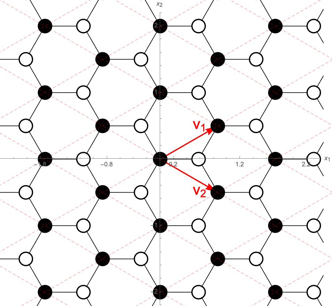
(a) Hexagonal lattice

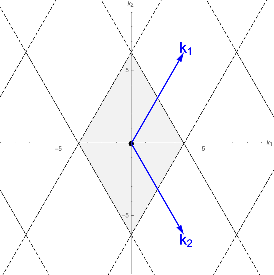
(b) Frequency domain

Figure 1.1. Periodic structure of the honeycomb lattice $\mathbf{H}$

For such a $\mathbb{C}^{2}$-valued function, its Lebesgue norm is defined as

$$\|\mathbf{u}\|_{L_{\mathbf{x}}^{r}}=\|\mathbf{u}\|_{L_{\mathbf{x}}^{r}(\mathbf{\Lambda};\mathbb{C}^{2})}=\begin{cases}\Big{(}\frac{\sqrt{3}}{2}\sum_{\mathbf{x}\in\mathbf{\Lambda}}|\mathbf{u}(\mathbf{x})|^{r}\Big{)}^{\frac{1}{r}}\quad&\text{ if }1\leq r<\infty,\\ \sup_{\mathbf{x}\in\mathbf{\Lambda}}|\mathbf{u}(\mathbf{x})|\quad&\text{ if }r=\infty,\end{cases}$$ (1.2)

where $|\mathbf{u}|=\sqrt{|u_{\bullet}|^{2}+|u_{\circ}|^{2}}$. The Fourier transform on the honeycomb lattice $\mathbf{H}$ is defined based on the group structure of the sub-lattice $\mathbf{\Lambda}$ as follows. Let

$$\mathbf{k}_{1}=\frac{4\pi}{\sqrt{3}}\begin{bmatrix}\cos\frac{\pi}{3}\\ \sin\frac{\pi}{3}\end{bmatrix}=\begin{bmatrix}\frac{2\pi}{\sqrt{3}}\\ 2\pi\end{bmatrix}\quad\textup{and}\quad\mathbf{k}_{2}=\frac{4\pi}{\sqrt{3}}\begin{bmatrix}\cos(-\frac{\pi}{3})\\ \sin(-\frac{\pi}{3})\end{bmatrix}=\begin{bmatrix}\frac{2\pi}{\sqrt{3}}\\ -2\pi\end{bmatrix}$$

be the reciprocal lattice vectors such that $\mathbf{v}_{i}\cdot\mathbf{k}_{j}=2\pi\delta_{ij}$, and define the dual periodic lattice by

$$\mathbf{\Lambda}^{*}:=\mathbb{Z}\mathbf{k}_{1}\oplus\mathbb{Z}\mathbf{k}_{2}.$$

Definition 1.1 (Fourier transform on the sub-lattice $\mathbf{\Lambda}$).

$(i)$ For a scalar-valued function $f:\mathbf{\Lambda}\to\mathbb{C}$, the Fourier transform is defined by

$$\hat{f}(\mathbf{k})=\frac{\sqrt{3}}{2}\sum_{\mathbf{x}\in\mathbf{\Lambda}}f(\mathbf{x})e^{-i\mathbf{k}\cdot\mathbf{x}}:\mathbb{R}^{2}/\mathbf{\Lambda}^{*}\to\mathbb{C},$$

and the inverse Fourier transform of $g:\mathbb{R}^{2}/\mathbf{\Lambda}^{*}\to\mathbb{C}$ is defined by

$$\check{g}(\mathbf{x})=\frac{1}{(2\pi)^{2}}\int_{\mathbb{R}^{2}/\mathbf{\Lambda}^{*}}g(\mathbf{k})e^{i\mathbf{k}\cdot\mathbf{x}}d\mathbf{k}:\mathbf{\Lambda}\to\mathbb{C}.$$

$(ii)$ For a $\mathbb{C}^{2}$-valued function $\mathbf{f}=(f_{\bullet},f_{\circ}):\mathbf{\Lambda}\to\mathbb{C}^{2}$ (resp., $\mathbf{g}=(g_{\bullet},g_{\circ}):\mathbb{R}^{2}/\mathbf{\Lambda}^{*}\to\mathbb{C}^{2}$), the Fourier transform (resp., the inverse Fourier transform) is defined by

$$\hat{\mathbf{f}}=(\hat{f}_{\bullet},\hat{f}_{\circ})\quad\Big{(}\textup{resp., }\check{\mathbf{g}}=(\check{g}_{\bullet},\check{g}_{\circ})\Big{)}.$$

Remark 1.2.

$(i)$ The frequency domain $\mathbb{R}^{2}/\mathbf{\Lambda}^{*}$ can be identified with the primitive rhombic cell, the gray region in Figure 1.1 (B) with the periodic boundary condition

$$\mathcal{B}_{\textup{rhom}}=\bigg{\{}s_{1}\mathbf{k}_{1}+s_{2}\mathbf{k}_{2}:-\frac{1}{2}<s_{1},s_{2}\leq\frac{1}{2}\bigg{\}}.$$ (1.3)

$(ii)$ In Definition 1.1, with a slight abuse of notation, we use the same symbols $\hat{\ }$ and $\check{\ }$ for both scalar-valued and $\mathbb{C}^{2}$-valued functions, but we distinguish them expressing $\mathbb{C}^{2}$-valued functions in bold, e.g. $\hat{\mathbf{f}}$ and $\check{\mathbf{g}}$.

On the honeycomb lattice $\mathbf{H}$, the dynamics of free waves is governed by the Schrödinger equation

$$i\partial_{t}u=-\Delta_{\mathbf{H}}u,$$

where $u:\mathbb{R}\times\mathbf{H}\to\mathbb{C}$ and $\Delta_{\mathbf{H}}$ denotes the standard discrete Laplacian for nearest neighbors. By (1.1), this scalar-valued equation can be identified with the $\mathbb{C}^{2}$-valued linear Schrödinger equation on the reduced periodic lattice $\mathbf{\Lambda}$, that is,

$$i\partial_{t}\mathbf{u}=-\mathbf{\Delta}\mathbf{u},$$ (1.4)

where

$$\mathbf{u}=\mathbf{u}(t,\mathbf{x}):\mathbb{R}\times\mathbf{\Lambda}\to\mathbb{C}^{2}$$

and $\mathbf{\Delta}$ is the vector-valued discrete Laplacian given by

$$(\mathbf{\Delta}\mathbf{u})(\mathbf{x})=4\begin{bmatrix}u_{\circ}(\mathbf{x})+u_{\circ}(\mathbf{x}-\mathbf{v}_{1})+u_{\circ}(\mathbf{x}-\mathbf{v}_{2})-3u_{\bullet}(\mathbf{x})\\ u_{\bullet}(\mathbf{x})+u_{\bullet}(\mathbf{x}+\mathbf{v}_{1})+u_{\bullet}(\mathbf{x}+\mathbf{v}_{2})-3u_{\circ}(\mathbf{x})\end{bmatrix},\quad\mathbf{u}=\begin{bmatrix}u_{\bullet}\\ u_{\circ}\end{bmatrix}:\mathbf{\Lambda}\to\mathbb{C}^{2}.$$ (1.5)

Then, the solution to the equation (1.4) with initial data $\mathbf{u}_{0}$ can be expressed as

$$\boxed{\quad e^{it\mathbf{\Delta}}\mathbf{u}_{0}=e^{-12it}\mathbf{O}(i\nabla_{\mathbf{x}})\begin{bmatrix}e^{-4it\varphi(i\nabla_{\mathbf{x}})}&0\\ 0&e^{4it\varphi(i\nabla_{\mathbf{x}})}\end{bmatrix}\mathbf{O}(i\nabla_{\mathbf{x}})^{*}\mathbf{u}_{0},\quad}$$ (1.6)

where $\varphi(i\nabla_{\mathbf{x}})$ is the scalar-valued Fourier multiplier with symbol

$$\varphi(\mathbf{k})=|z(\mathbf{k})|=\sqrt{3+2\cos(\mathbf{k}\cdot\mathbf{v}_{1})+2\cos(\mathbf{k}\cdot\mathbf{v}_{2})+2\cos(\mathbf{k}\cdot(\mathbf{v}_{1}-\mathbf{v}_{2}))}$$

with

$$z(\mathbf{k})=1+e^{i\mathbf{k}\cdot\mathbf{v}_{1}}+e^{i\mathbf{k}\cdot\mathbf{v}_{2}}$$

and $\mathbf{O}(i\nabla_{\mathbf{x}})$ is the vector-valued Fourier multiplier with symbol with

$$\mathbf{O}(\mathbf{k})=\begin{bmatrix}\ \frac{1}{\sqrt{2}}&\frac{\overline{z(\mathbf{k})}}{\sqrt{2}|z(\mathbf{k})|}\\ -\frac{z(\mathbf{k})}{\sqrt{2}|z(\mathbf{k})|}&\frac{1}{\sqrt{2}}\end{bmatrix}$$

(see Appendix A for the derivation of the formula (1.6)).

Remark 1.3.

By Parseval’s theorem, $\mathbf{O}(i\nabla_{\mathbf{x}})$ is unitary on $L^{2}(\mathbf{\Lambda};\mathbb{C}^{2})$. Moreover, it is bounded on $L^{p}(\mathbf{\Lambda};\mathbb{C}^{2})$ with $1<p<\infty$ (see Lemma B.1).

By the representation (1.6), the dynamics of the Schrödinger flow $e^{it\mathbf{\Delta}}\mathbf{u}_{0}$ is completely determined by the geometric stucture of the frequency surfaces

$$\mathcal{S}_{\pm}=\Big{\{}\big{(}\mathbf{k},\pm\varphi(\mathbf{k})\big{)}:\mathbf{k}\in\mathbb{R}^{2}/\mathbf{\Lambda}^{*}\Big{\}}.$$ (1.7)

Note that the two surfaces meet, or $\varphi(\mathbf{k})=0$, called Dirac points. In fact, the Dirac points are the two points $[0\ \pm\frac{4\pi}{3}]^{\textup{T}}+\mathbf{\Lambda}^{*}$ in the primitive rhombic zone $\mathcal{B}_{\textup{rhom}}$ (see (1.3) and Figure 2.1). It is well known that the frequency surfaces $\mathcal{S}_{\pm}$ have a conical singularity at a Dirac point $\mathbf{K}_{\star}$. By Fefferman, Lee-Thorp and Weinstein [25], it is shown that in the tight-binding regime, the first two lowest energy bands for the continuum model converge to $\pm\varphi(\mathbf{k})$ uniformly in $\mathbf{k}$.

2. Main results

The purpose of this article is to investigate the detailed dispersive properties of wave propagation in a honeycomb lattice, depending on frequency localization. In a cubic lattice, $L^{1}\to L^{\infty}$ dispersion bounds have been established for discrete Schrödinger, Klein-Gordon and wave equations; [21, 48, 53] for a one-dimensional lattice, and [9, 10, 11, 31, 16, 56, 57] for multi-dimensional lattices. Such time decay estimates are a fundamental tool for studying discrete dispersive equations in various aspects. For example, they have been used to nonlinear problems, including the continuum limit of discrete models [14, 15, 32, 33, 34, 35, 36, 37, 38, 39, 46, 65]. We also note that in a similar context, uniform resolvent estimates of discrete Schrödinger operators on a cubic lattice are proved [17, 60, 61, 62], but the spectral and scattering properties of discrete Schrödinger operators on honeycomb (and general) lattices are also considered in [4, 5, 52, 59]. However, to the best of the authors’ knowledge, the dispersion estimate on a honeycomb lattice has not yet been known, despite its physical importance.

2.1. Characterization of degenerate frequencies

By the representation (1.6), the time-decay of the Schrödinger flow $e^{it\mathbf{\Delta}}\mathbf{u}_{0}$ is determined by the phase function

$$\boxed{\quad\varphi(\mathbf{k})=\sqrt{3+2\cos(\mathbf{k}\cdot\mathbf{v}_{1})+2\cos(\mathbf{k}\cdot\mathbf{v}_{2})+2\cos(\mathbf{k}\cdot(\mathbf{v}_{1}-\mathbf{v}_{2}))}\quad}$$ (2.1)

where $\mathbf{v}_{1}=(\frac{\sqrt{3}}{2},\frac{1}{2})$ and $\mathbf{v}_{2}=(\frac{\sqrt{3}}{2},-\frac{1}{2})$. In order to find the precise dispersion rate, a crucial step is to compute the local series expansions of the phase.

Our first main result provides the explicit formulae for the Hessian of the phase $\varphi(\mathbf{k})$ and its determinant, given by the three periodic functions

$$\left\{\begin{aligned} \alpha_{1}(\mathbf{k})&:=1+\cos(\mathbf{k}\cdot\mathbf{v}_{2})+\cos(\mathbf{k}\cdot(\mathbf{v}_{1}-\mathbf{v}_{2})),\\ \alpha_{2}(\mathbf{k})&:=1+\cos(\mathbf{k}\cdot\mathbf{v}_{1})+\cos(\mathbf{k}\cdot(\mathbf{v}_{1}-\mathbf{v}_{2})),\\ \alpha_{12}(\mathbf{k})&:=1+\cos(\mathbf{k}\cdot\mathbf{v}_{1})+\cos(\mathbf{k}\cdot\mathbf{v}_{2}),\end{aligned}\right.$$ (2.2)

from which degenerate frequencies are completely characterized by the three periodic curves.

Theorem 2.1 (Characterization of degenerate frequencies).

For any frequency $\mathbf{k}\in\mathbb{R}^{2}/\mathbf{\Lambda}^{*}$ such that $\varphi(\mathbf{k})\neq 0$, i.e, $\mathbf{k}$ is not a Dirac point, we have

$$(\nabla^{2}\varphi)(\mathbf{k})=\frac{1}{\varphi(\mathbf{k})^{3}}\mathbf{V}\begin{bmatrix}-\alpha_{2}(\mathbf{k})(\alpha_{1}(\mathbf{k})+\alpha_{12}(\mathbf{k}))&\alpha_{1}(\mathbf{k})\alpha_{2}(\mathbf{k})\\ \alpha_{1}(\mathbf{k})\alpha_{2}(\mathbf{k})&-\alpha_{1}(\mathbf{k})(\alpha_{2}(\mathbf{k})+\alpha_{12}(\mathbf{k}))\end{bmatrix}\mathbf{V}^{\textup{T}},$$

where $\mathbf{V}=[\mathbf{v}_{1}\ \mathbf{v}_{2}]$, and

$$\textup{det}(\nabla^{2}\varphi)(\mathbf{k})=\frac{3\alpha_{1}(\mathbf{k})\alpha_{2}(\mathbf{k})\alpha_{12}(\mathbf{k})}{4\varphi(\mathbf{k})^{4}}.$$ (2.3)

As a consequence, $\textup{det}(\nabla^{2}\varphi)(\mathbf{k})=0$ if and only if

$$\alpha_{1}(\mathbf{k})=0,\quad\alpha_{2}(\mathbf{k})=0\quad\textup{or}\quad\alpha_{12}(\mathbf{k})=0.$$

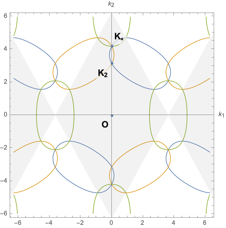
Figure 2.1. Degenerate frequency curves.

Remark 2.2.

$(i)$ Theorem 2.1 provides more detailed geometric information of the well-known frequency surfaces $\mathcal{S}_{\pm}$ for the tight-binding model of graphene. To the best of authors’ knowledge, this is the first result for the classification of degenerate frequencies of the phase $\varphi(\mathbf{k})$.
$(ii)$ Notably, the determinant of the Hessian (2.3) is factorizable. From Figure 2.1, we observe that the degenerate frequencies are located on the three simple periodic curves $\alpha_{1}(\mathbf{k})=0$, $\alpha_{2}(\mathbf{k})=0$ and $\alpha_{12}(\mathbf{k})=0$ with symmetry; the three degenerate frequency curves are symmetric under 60 degree rotation. Moreover, all three curves intersect only at Dirac points. These facts are completely non-trivial, and relies heavily on the symmetric algebraic structure of the graphene lattice model. Indeed, it is not easy to expect factorization of $\textup{det}(\nabla^{2}\varphi)(\mathbf{k})$ a priori-ly, because the direct expansion of $\textup{det}(\nabla^{2}\varphi)(\mathbf{k})$ has many rational functions of trigonometric functions, and it is too difficult to reorganize them using the trigonometric identities by hands. The “magical” formula (2.3) was obtained unexpectedly by Mathematica-aided computations. Note also that for non-symmetric hexagonal latice models, for example, that for boron nitrides [55], the phase function does not have a similar factorization property.
$(iii)$ The notation (2.2) has symmetry in that $\alpha_{j}(\mathbf{k})=\frac{\varphi(\mathbf{k})^{2}-1}{2}-\cos(\mathbf{k}\cdot\mathbf{v}_{j})$ for $j=1,2$, and $\alpha_{12}(\mathbf{k})=\frac{\varphi(\mathbf{k})^{2}-1}{2}-\cos(\mathbf{k}\cdot(\mathbf{v}_{1}-\mathbf{v}_{2}))$.

By Theorem 2.1, the periodic frequency domain is decomposed as

$$\mathbb{R}^{2}/\mathbf{\Lambda}^{*}=\bigsqcup_{j=0}^{3}\mathcal{K}_{j},$$

where $\mathcal{K}_{j}$ denotes the set of intersections of $j$-many frequency curves, precisely,

$$\mathcal{K}_{0} =\Big{\{}\mathbf{k}\in(\mathbb{R}^{2}/\mathbf{\Lambda}^{*})\setminus\mathcal{K}_{3}:\textup{det}(\nabla^{2}\varphi)(\mathbf{k})\neq 0\Big{\}},$$ (2.4)

$$\mathcal{K}_{1} =\Big{\{}\mathbf{k}\in\mathbb{R}^{2}/\mathbf{\Lambda}^{*}:\textup{det}(\nabla^{2}\varphi)(\mathbf{k})=0\Big{\}}\setminus(\mathcal{K}_{2}\cup\mathcal{K}_{3}),$$

$$\mathcal{K}_{2} =\bigg{\{}\bigg{(}\frac{\sqrt{3}\pi}{2},\pm\frac{\pi}{2}\bigg{)},\bigg{(}\frac{\sqrt{3}\pi}{6},\pm\frac{3\pi}{2}\bigg{)},(0,\pm\pi)\bigg{\}}+\mathbf{\Lambda}^{*},$$

$$\mathcal{K}_{3} =\bigg{(}0,\pm\frac{4\pi}{3}\bigg{)}+\mathbf{\Lambda}^{*}\quad\textup{(Dirac points)}.$$

2.2. Dispersion and Strichartz estimates

Based on the characterization of degenerate frequencies (Theorem 2.1), we establish our second main result, that is, the dispersion estimates for the Schrödinger flow on the honeycomb lattice $\mathbf{H}$, whose decay rate depends on frequency localization.

Theorem 2.3 (Frequency localized dispersion estimates).

For each $\mathbf{K}\in\mathcal{K}_{j}$ with $j=0,1,2,3$, there exist $C_{j}=C_{j}(\mathbf{K})>0$ and a smooth cut-off $\chi_{\approx\mathbf{K}}$ such that $\chi_{\approx\mathbf{K}}$ is supported in a sufficiently small neighborhood of $\mathbf{K}$, $\chi_{\approx\mathbf{K}}=1$ near $\mathbf{K}$, and

$$\|\mathbf{O}(i\nabla_{\mathbf{x}})^{*}e^{it\mathbf{\Delta}}\mathbf{O}(i\nabla_{\mathbf{x}})P_{\approx\mathbf{K}}\mathbf{u}_{0}\|_{L_{\mathbf{x}}^{\infty}(\mathbf{\Lambda};\mathbb{C}^{2})}\leq\frac{C_{j}}{(1+|t|)^{a_{j}}}\|\mathbf{u}_{0}\|_{L_{\mathbf{x}}^{1}(\mathbf{\Lambda};\mathbb{C}^{2})},$$ (2.5)

where $\mathbf{O}(i\nabla_{\mathbf{x}})$ is given by (1.6), $P_{\approx\mathbf{K}}$ is the Fourier multiplier with symbol $\chi_{\approx\mathbf{K}}$, that is, $\widehat{P_{\approx\mathbf{K}}u}(\mathbf{k})=\chi_{\approx\mathbf{K}}(\mathbf{k})\hat{u}(\mathbf{k})$, and

$$a_{j}=\left\{\begin{aligned} &1&&\textup{if }j=0,\\ &\tfrac{5}{6}&&\textup{if }j=1,\\ &\tfrac{2}{3}&&\textup{if }j=2,\\ &\tfrac{5}{6}&&\textup{if }j=3.\end{aligned}\right.$$ (2.6)

Remark 2.4 (Decay rate).

$(i)$ The slowest $O(|t|^{-2/3})$-decay rate is obtained at the intersections of two degenerate frequency curves, not at Dirac points.
$(ii)$ Near Dirac points, even though the frequency surfaces $\mathcal{S}_{\pm}$ (see (1.7)) are asymptotically conic, the faster $O(|t|^{-5/6})$-dispersion rate is obtained compare to the $O(|t|^{-1/2})$-decay rate for the standard linear wave equation on $\mathbb{R}^{2}$. Indeed, the phase $\varphi(\mathbf{k})$ behaves like that for the wave equation, precisely, $\varphi(\mathbf{k})\approx\frac{\sqrt{3}}{2}|\mathbf{K}+\mathbf{k}|$ but only in the leading order. The faster decay can be captured from the additional oscillation by higher-order terms (see Lemma 5.6 and 5.11). For the discrete wave equation, a similar faster decay has already been discovered in Schultz [56].
$(iii)$ The inequality (2.5) is not scaling-invariant, because the lattice spacing of the domain $\mathbf{\Lambda}$ is fixed. Indeed, in the physically important scaling limit regime with strong localization at a Dirac point, we do not expect a uniform decay rate faster than $O(|t|^{-1/2})$, because the inequality (2.5) must also be scaled to have coefficients that blow up in the limit.

Remark 2.5 (Non-degenerate frequency case $j=0$).

For each $\mathbf{K}\in\mathcal{K}_{0}$, one can choose a smooth cut-off $\chi_{\approx\mathbf{K}}$ with sufficiently small support where the phase is non-degenerate. Thus, the standard oscillatory integral estimate yields Theorem 2.3 with $j=0$.

Remark 2.6 (Degenerate frequency case $j=1,2,3$; direct proof).

$(i)$ If $\mathbf{K}$ is located on a degenerate frequency curve, then a more delicate analysis is required. Indeed, when $\mathbf{K}\in\mathcal{K}_{1}\cup\mathcal{K}_{2}$, one may employ the theory of oscillatory integrals with degenerate phases such as celebrated Varchenko’s theorem [63] relating Newton polygons and asymptotics of the oscillatory integrals, and Karpushkin’s theorem [41, 42] for stability of oscillatory integrals (see also [20, 40, 54]). However, the known theories sometimes refer to other known theories, e.g., resolution of singularities [30], or unfoldings of singularities [7], with which many researchers are not familiar. For this reason, in this article, a direct proof is provided involving elementary integration by parts and changes of variables.
$(ii)$ Another benefit of a direct proof is that the physically most interesting case $\mathbf{K}\in\mathcal{K}_{3}$ can also be treated in a similar way. Note that near a Dirac point, the phase function is not only degenerate but also non-differentiable as the frequency surface is asymptotically conic. However, most known oscillatory integral theories require some regularity of phases.
$(iii)$ Our direct proof is based on the robust technique to show dispersion estimates for the wave-type equations [51, 58].

By compactness of the frequency domain $\mathbb{R}^{2}/\mathbf{\Lambda}^{*}$, collecting all and interpolating with the unitarity of the flow $e^{it\mathbf{\Delta}}$, we obtain the dispersion estimate without frequency localization.

Corollary 2.7 (Dispersion estimate).

For $r\geq 2$, we have

$$\|\mathbf{O}(i\nabla_{\mathbf{x}})^{*}e^{it\mathbf{\Delta}}\mathbf{u}_{0}\|_{L_{\mathbf{x}}^{r}(\mathbf{\Lambda};\mathbb{C}^{2})}\lesssim\frac{1}{(1+|t|)^{\frac{4}{3}(\frac{1}{2}-\frac{1}{r})}}\|\mathbf{O}(i\nabla_{\mathbf{x}})^{*}\mathbf{u}_{0}\|_{L_{\mathbf{x}}^{r^{\prime}}(\mathbf{\Lambda};\mathbb{C}^{2})}.$$

As a consequence, employing the standard interpolation argument [44], we deduce Strichartz estimates. We call $(q,r)$ an admissible pair if

$$\frac{3}{q}+\frac{2}{r}=1\quad\textup{and}\quad 2\leq q,r\leq\infty.$$

Corollary 2.8 (Strichartz estimates).

For admissible pairs $(q,r)$ and $(\tilde{q},\tilde{r})$, we have

$$\|\mathbf{O}(i\nabla_{\mathbf{x}})^{*}e^{it\mathbf{\Delta}}\mathbf{u}_{0}\|_{L_{t}^{q}(\mathbb{R};L_{\mathbf{x}}^{r}(\mathbf{\Lambda};\mathbb{C}^{2}))}\lesssim\|\mathbf{u}_{0}\|_{L_{\mathbf{x}}^{2}(\mathbf{\Lambda};\mathbb{C}^{2})}$$ (2.7)

and

$$\bigg{\|}\mathbf{O}(i\nabla_{\mathbf{x}})^{*}\int_{0}^{t}e^{i(t-t^{\prime})\mathbf{\Delta}}\mathbf{F}(t^{\prime})dt^{\prime}\bigg{\|}_{L_{t}^{q}(\mathbb{R};L_{\mathbf{x}}^{r}(\mathbf{\Lambda};\mathbb{C}^{2}))}\lesssim\|\mathbf{O}(i\nabla_{\mathbf{x}})^{*}\mathbf{F}\|_{L_{t}^{\tilde{q}^{\prime}}(\mathbb{R};L_{\mathbf{x}}^{\tilde{r}^{\prime}}(\mathbf{\Lambda};\mathbb{C}^{2}))}.$$ (2.8)

Remark 2.9.

In Corollary 2.7 and 2.8, we may drop $\mathbf{O}(i\nabla_{\mathbf{x}})^{*}$ provided that $r,\tilde{r}\neq\infty$, because $\mathbf{O}(i\nabla_{\mathbf{x}})^{*}$ is bounded on $L^{r}(\mathbf{\Lambda};\mathbb{C}^{2}))$ for $1<r<\infty$ (see Lemma B.1).

2.3. Nonlinear application

As a simple application of our main linear estimates, we establish the small data scattering for the nonlinear Schrödinger equation on the reduced periodic lattice $\mathbf{\Lambda}$ with a power-type nonlinearity

$$i\partial_{t}\mathbf{u}=-\mathbf{\Delta}\mathbf{u}+\mathcal{N}(\mathbf{u}),$$ (2.9)

where

$$\mathbf{u}=\mathbf{u}(t,\mathbf{x})=\begin{bmatrix}u_{\bullet}(t,\mathbf{x})\\ u_{\circ}(t,\mathbf{x})\end{bmatrix}:\mathbb{R}\times\mathbf{\Lambda}\to\mathbb{C}^{2}$$

and the nonlinear term is given by

$$\mathcal{N}(\mathbf{u})=\pm\begin{bmatrix}|u_{\bullet}|^{p-1}u_{\bullet}\\ |u_{\circ}|^{p-1}u_{\circ}\end{bmatrix}=\pm\begin{bmatrix}|u_{\bullet}|^{p-1}&0\\ 0&|u_{\circ}|^{p-1}\end{bmatrix}\mathbf{u}.$$

Theorem 2.10 (Small data scattering).

Suppose that $r>2$, $p>3+\max(\frac{3}{r-2}-\frac{3}{2},\frac{1}{2}-\frac{2}{r})$ and $\|\mathbf{u}_{0}\|_{L_{\mathbf{x}}^{r^{\prime}}(\mathbf{\Lambda};\mathbb{C}^{2})}\leq\epsilon_{0}$ for sufficiently small $\epsilon_{0}>0$. Then, the Cauchy problem with initial data $\mathbf{u}_{0}$ has a unique global solution satisfying

$$\sup_{t\in\mathbb{R}}\Big{\{}(1+|t|)^{\frac{4}{3}(\frac{1}{2}-\frac{1}{r})}\|\mathbf{u}(t)\|_{L_{\mathbf{x}}^{r}(\mathbf{\Lambda};\mathbb{C}^{2})}\Big{\}}\lesssim\|\mathbf{u}_{0}\|_{L_{\mathbf{x}}^{r^{\prime}}(\mathbf{\Lambda};\mathbb{C}^{2})}.$$ (2.10)

Furthermore, there exists a forward-in-time (resp., backward-in-time) scattering states $\mathbf{u}_{+}\in L_{\mathbf{x}}^{2}(\mathbf{\Lambda};\mathbb{C}^{2})$ (resp., $\mathbf{u}_{-}\in L_{\mathbf{x}}^{2}(\mathbf{\Lambda};\mathbb{C}^{2})$) such that for $t\geq 1$ (resp., $t\leq-1$), then

$$\|e^{-it\mathbf{\Delta}}\mathbf{u}(t)-\mathbf{u}_{\pm}\|_{L_{\mathbf{x}}^{2}(\mathbf{\Lambda};\mathbb{C}^{2})}\lesssim\frac{\|\mathbf{u}_{0}\|_{L_{\mathbf{x}}^{r^{\prime}}(\mathbf{\Lambda};\mathbb{C}^{2})}^{p}}{(1+|t|)^{\sigma_{r,p}-1}},$$ (2.11)

where

$$\sigma_{r,p}:=\left\{\begin{aligned} &\frac{4}{3}\bigg{(}\frac{1}{2}-\frac{1}{r}\bigg{)}p&&\text{if }p\geq r-1,\\ &\frac{4}{3}\bigg{(}\frac{1}{2}-\frac{1}{r^{\prime}p}\bigg{)}p&&\text{if }p<r-1.\end{aligned}\right.$$ (2.12)

Remark 2.11.

$(i)$ Theorem 2.10 includes super-cubic nonlinearities, i.e., $p>3$. Note that for the assumption on $p$, the minimum value of $3+\max(\frac{3}{r-2}-\frac{3}{2},\frac{1}{2}-\frac{2}{r})$ is attained when $r=4$, and it is $3$. Indeed, by the time decay rate (Corollary 2.7), it is natural to conjecture that small data scattering holds if $p>\frac{5}{2}=1+\frac{3}{2}$. The gap is due to the lack of the vector-field identity in the discrete setting.
$(ii)$ If one employs a weaker $O(|t|^{-1/2})$ wave-like $L^{1}\to L^{\infty}$ dispersion bound from the crude estimate (Proposition 5.8), a similar small data scattering can be obtained, but the range of nonlinearities is restricted to $p>\max(2+\frac{4}{r-2},4-\frac{2}{r})$, with $p>\frac{3+\sqrt{17}}{2}$.

2.4. Notations

Throughout this article, we denote $A\lesssim B$ (resp., $A\gtrsim B$, or $A\sim B$) if there exists $C\geq 1$ such that $A\leq CB$ (resp., $A\geq CB$, or $\frac{1}{C}A\leq B\leq CA$). If the implicit constant $C\geq 1$ depends on some other parameter $a$, then we denote by $A\lesssim_{a}B$, $A\gtrsim_{a}B$, or $A\sim_{a}B$. However, if such dependence is not essential in analysis, the subscript $a$ is omitted. It is important to note that in any case, the implicit constants do not depend on $t\in\mathbb{R}$ and the specific choice of $\mathbf{x}$.

Let $\chi_{0}:\mathbb{R}\to[0,\infty)$ be a smooth cut-off such that

$$\chi_{0}(s)=\left\{\begin{aligned} &1&&\textup{if }|s|\leq\tfrac{1}{2},\\ &0&&\textup{if }|s|\geq 1,\end{aligned}\right.$$ (2.13)

and define

$$\chi_{1}:=1-\chi_{0}.$$ (2.14)

For the Littlewood-Paley theory, we choose a standard smooth cut-off

$$\eta:\mathbb{R}\to[0,1]$$ (2.15)

such that $\eta\equiv 1$ on $[\frac{6}{5},\frac{9}{5}]$, $\eta\equiv 0$ outside $[\frac{4}{5},\frac{11}{5}]$ and $\sum_{N\in 2^{\mathbb{Z}}}\eta(\frac{\cdot}{N})\equiv 1$. Replacing $\chi_{0}(\frac{\cdot}{\delta})$ by $\sum_{N\leq\delta}\eta(\frac{\cdot}{N})$ if necessary, we may assume that $\chi_{0}(\frac{\cdot}{\delta})=\sum_{N\leq\delta}\eta(\frac{\cdot}{N})$.

For a non-negative integer $m$, let $\mathcal{O}_{m}(\mathbf{k})$ denote an analytic function near the origin such that $|\mathcal{O}_{m}(\mathbf{k})|\lesssim|\mathbf{k}|^{m}$ and is of the form

$$\mathcal{O}_{m}(\mathbf{k})=\sum_{m_{1}+m_{2}\geq m}c_{m_{1},m_{2}}k_{1}^{m_{1}}k_{2}^{m_{2}}.$$ (2.16)

In most situations, the specific choice of the coefficients in (2.16) is not essential, but only their bounds are important. If this is the case, abusing notations, we express any such analytic functions by $\mathcal{O}_{m}(\mathbf{k})$ rather than introducing more notations like $\tilde{\mathcal{O}}_{m}(\mathbf{k})$, $\tilde{\tilde{\mathcal{O}}}_{m}(\mathbf{k})$, …

2.5. Organization of the paper

The rest of the paper is organized as follows. In Section 3, we give a proof of the first main result (Theorem 2.1). The next four sections are devoted to the proof of the dispersion estimate (Theorem 2.3). In Section 4, we reduce the proof of the dispersion estimate to that of the degenerate phase oscillatory integral estimate. Then, in Sections 5, 6 and 7, we prove the oscillatory integral bound corresponding to the case $\mathbf{K}\in\mathcal{K}_{j}$ with $j=3,2,1$, respectively. In Section 8, we prove small data scattering (Theorem 2.10). In Appendix A and B, we provide the proof of the factorization formula of the linear flow (1.6) and that of the boundedness of the operator $\mathbf{O}(i\nabla_{\mathbf{x}})$ (Lemma B.1).

2.6. Acknowledgment

Y. Hong was supported by National Research Foundation of Korea (NRF) grant funded by the Korean government (MSIT) (No. RS-2023-00208824, No. RS-2023-00219980). Y. Tadano was supported by by JSPS KAKENHI Grant Number JP23K12991. C. Yang was supported by the National Research Foundation of Korea (NRF) grant funded by the Korea government (MSIT) (No. 2021R1C1C1005700). The authors would like to thank Professor Sung-Jin Oh for explaining the integration by parts trick crucially used throughout this article.

3. Characterization of degenerate frequencies: Proof of Theorem 2.1

Introducing the new variable $\tilde{\mathbf{k}}=(\mathbf{k}\cdot\mathbf{v}_{1},\mathbf{k}\cdot\mathbf{v}_{2})=\mathbf{V}^{\textup{T}}\mathbf{k}$, we write the phase function in a simpler form as

$$\varphi(\mathbf{k})=\tilde{\varphi}(\tilde{\mathbf{k}}):=\sqrt{3+2\cos\tilde{k}_{1}+2\cos\tilde{k}_{2}+2\cos(\tilde{k}_{1}-\tilde{k}_{2})}.$$

Then, it suffices to show that

$$\nabla_{\tilde{\mathbf{k}}}^{2}\tilde{\varphi}=\frac{1}{\tilde{\varphi}^{3}}\begin{bmatrix}-\tilde{\alpha}_{2}(\tilde{\alpha}_{1}+\tilde{\alpha}_{12})&\tilde{\alpha}_{1}\tilde{\alpha}_{2}\\ \tilde{\alpha}_{1}\tilde{\alpha}_{2}&-\tilde{\alpha}_{1}(\tilde{\alpha}_{2}+\tilde{\alpha}_{12}),\end{bmatrix}$$ (3.1)

where $\tilde{\alpha}_{1}=1+\cos\tilde{k}_{2}+\cos(\tilde{k}_{1}-\tilde{k}_{2})$, $\tilde{\alpha}_{2}=1+\cos\tilde{k}_{1}+\cos(\tilde{k}_{1}-\tilde{k}_{2})$ and $\tilde{\alpha}_{12}=1+\cos\tilde{k}_{1}+\cos\tilde{k}_{2}$, because together with the identity $\tilde{\varphi}^{2}=\tilde{\alpha}_{1}+\tilde{\alpha}_{2}+\tilde{\alpha}_{12}$, it implies that

$$\textup{det}(\nabla_{\tilde{\mathbf{k}}}^{2}\tilde{\varphi})=\frac{\tilde{\alpha}_{1}\tilde{\alpha}_{2}}{\tilde{\varphi}^{6}}\tilde{\alpha}_{12}(\tilde{\alpha}_{1}+\tilde{\alpha}_{2}+\tilde{\alpha}_{12})=\frac{\tilde{\alpha}_{1}\tilde{\alpha}_{2}\tilde{\alpha}_{12}}{\tilde{\varphi}^{4}}.$$

For the proof of (3.1), we compute

$$\nabla_{\tilde{\mathbf{k}}}\tilde{\varphi}=\bigg{(}-\frac{\sin\tilde{k}_{1}+\sin(\tilde{k}_{1}-\tilde{k}_{2})}{\tilde{\varphi}},-\frac{\sin\tilde{k}_{2}-\sin(\tilde{k}_{1}-\tilde{k}_{2})}{\tilde{\varphi}}\bigg{)}.$$

For the Hessian matrix, we calculate the second derivatives. Indeed, differentiating $\partial_{\tilde{k}_{1}}\tilde{\varphi}$, we obtain

$$\partial_{\tilde{k}_{1}}^{2}\tilde{\varphi}=-\frac{(\cos\tilde{k}_{1}+\cos(\tilde{k}_{1}-\tilde{k}_{2}))\tilde{\varphi}^{2}+(\sin\tilde{k}_{1}+\sin(\tilde{k}_{1}-\tilde{k}_{2}))^{2}}{\tilde{\varphi}^{3}}.$$ (3.2)

In (3.2), we simplify the numerator replacing all sine functions by cosines, but we also rearrange the terms in order of $c_{12}=\cos(\tilde{k}_{1}-\tilde{k}_{2})$. Indeed, the first term in the numerator can be written as

$$\big{(}\cos\tilde{k}_{1}+\cos(\tilde{k}_{1}-\tilde{k}_{2})\big{)}\tilde{\varphi}^{2} =(\cos\tilde{k}_{1}+c_{12})(3+2\cos\tilde{k}_{1}+2\cos\tilde{k}_{2}+2c_{12})$$

$$=2(c_{12})^{2}+(3+4\cos\tilde{k}_{1}+2\cos\tilde{k}_{2})c_{12}$$

$$\quad+2\cos^{2}\tilde{k}_{1}+(3+2\cos\tilde{k}_{2})\cos\tilde{k}_{1}.$$

For the second term, applying the angle-sum formula in the form

$$\sin\theta_{1}\sin\theta_{2}=\cos(\theta_{1}-\theta_{2})-\cos\theta_{1}\cos\theta_{2},$$ (3.3)

we obtain

$$\big{(}\sin\tilde{k}_{1}+\sin(\tilde{k}_{1}-\tilde{k}_{2})\big{)}^{2} =\sin^{2}\tilde{k}_{1}+\sin^{2}(\tilde{k}_{1}-\tilde{k}_{2})+2\sin\tilde{k}_{1}\sin(\tilde{k}_{1}-\tilde{k}_{2})$$

$$=(1-\cos^{2}\tilde{k}_{1})+(1-(c_{12})^{2})+2\big{(}\cos\tilde{k}_{2}-(\cos\tilde{k}_{1})c_{12}\big{)}$$

$$=-(c_{12})^{2}-2(\cos\tilde{k}_{1})c_{12}+(-\cos^{2}\tilde{k}_{1}+2\cos\tilde{k}_{2}+2).$$

Hence, summing them in (3.2), we obtain that

$$\partial_{\tilde{k}_{1}}^{2}\tilde{\varphi} =-\frac{(c_{12})^{2}+(3+2\cos\tilde{k}_{1}+2\cos\tilde{k}_{2})c_{12}+(\cos\tilde{k}_{1}+1)(\cos\tilde{k}_{1}+2\cos\tilde{k}_{2}+2)}{\tilde{\varphi}^{3}}$$

$$=-\frac{(c_{12}+\cos\tilde{k}_{1}+1)(c_{12}+\cos\tilde{k}_{1}+2\cos\tilde{k}_{2}+2)}{\tilde{\varphi}^{3}}=-\frac{\tilde{\alpha}_{2}(\tilde{\alpha}_{1}+\tilde{\alpha}_{12})}{\tilde{\varphi}^{3}}.$$

By symmetry, switching the roles of $\tilde{k}_{1}$ and $\tilde{k}_{2}$, we prove that $\partial_{\tilde{k}_{2}}^{2}\tilde{\varphi}=-\frac{\tilde{\alpha}_{1}(\tilde{\alpha}_{2}+\tilde{\alpha}_{12})}{\tilde{\varphi}^{3}}$.

It remains to compute $\partial_{\tilde{k}_{1}}\partial_{\tilde{k}_{2}}\tilde{\varphi}$. Indeed, we have

$$\partial_{\tilde{k}_{1}}\partial_{\tilde{k}_{2}}\tilde{\varphi}=\frac{\cos(\tilde{k}_{1}-\tilde{k}_{2})\tilde{\varphi}^{2}-(\sin\tilde{k}_{1}+\sin(\tilde{k}_{1}-\tilde{k}_{2}))(\sin\tilde{k}_{2}-\sin(\tilde{k}_{1}-\tilde{k}_{2}))}{\tilde{\varphi}^{3}}.$$

We again replace sines by cosines in the numerator using (3.3),

$$\cos(\tilde{k}_{1}-\tilde{k}_{2})\tilde{\varphi}^{2}-(\sin\tilde{k}_{1}+\sin(\tilde{k}_{1}-\tilde{k}_{2}))(\sin\tilde{k}_{2}-\sin(\tilde{k}_{1}-\tilde{k}_{2}))$$

$$=\cos(\tilde{k}_{1}-\tilde{k}_{2})\tilde{\varphi}^{2}-\sin\tilde{k}_{1}\sin\tilde{k}_{2}+\sin\tilde{k}_{1}\sin(\tilde{k}_{1}-\tilde{k}_{2})+\sin(\tilde{k}_{2}-\tilde{k}_{1})\sin\tilde{k}_{2}+\sin^{2}(\tilde{k}_{1}-\tilde{k}_{2})$$

$$=c_{12}(3+2\cos\tilde{k}_{1}+2\cos\tilde{k}_{2}+2c_{12})-(c_{12}-\cos\tilde{k}_{1}\cos\tilde{k}_{2})+(\cos\tilde{k}_{2}-(\cos\tilde{k}_{1})c_{12})$$

$$\quad+(\cos\tilde{k}_{1}-c_{12}\cos\tilde{k}_{2})+1-(c_{12})^{2},$$

where $c_{12}=\cos(\tilde{k}_{1}-\tilde{k}_{2})$. Then, we arrange terms in order of $c_{12}$ as follows,

$$\partial_{\tilde{k}_{1}}\partial_{\tilde{k}_{2}}\tilde{\varphi} =\frac{(c_{12})^{2}+(2+\cos\tilde{k}_{1}+\cos\tilde{k}_{2})c_{12}+(1+\cos\tilde{k}_{1})(1+\cos\tilde{k}_{2})}{\tilde{\varphi}^{3}}$$

$$=\frac{(c_{12}+1+\cos\tilde{k}_{1})(c_{12}+1+\cos\tilde{k}_{2})}{\tilde{\varphi}^{3}}=\frac{\tilde{\alpha}_{1}\tilde{\alpha}_{2}}{\tilde{\varphi}^{3}}.$$

Therefore, collecting all, we prove (3.1).

4. Reduction to the oscillatory integral estimate

By the factorization structure (1.6), the core part of the frequency localized Schrödinger flow $e^{it\mathbf{\Delta}}P_{\approx\mathbf{K}}\mathbf{u_{0}}$ is given by the scalar-valued flow $e^{it\varphi(-i\mathbf{\nabla}_{\mathbf{x}})}P_{\approx\mathbf{K}}u_{0}$, that is, the Fourier multiplier such that

$$(e^{-it\varphi(-i\mathbf{\nabla}_{\mathbf{x}})}P_{\approx\mathbf{K}}u_{0})^{\wedge}(\mathbf{k})=e^{-it\varphi(\mathbf{k})}\chi_{\approx\mathbf{K}}(\mathbf{k})\hat{u}_{0}(\mathbf{k}),$$

where $\varphi(\mathbf{k})$ is the phase function given in (2.1) and $u_{0}:\mathbf{\Lambda}\to\mathbb{C}$ is scalar. Thus, by the Fourier transform (see Definition 1.1), the scalar flow has the integral representation

$$(e^{-it\varphi(-i\mathbf{\nabla}_{\mathbf{x}})}u_{0})(\mathbf{x})=\frac{\sqrt{3}}{8\pi^{2}}\sum_{\mathbf{y}\in\mathbf{\Lambda}}\mathbb{I}_{\mathbf{k}\approx\mathbf{K}}\bigg{(}t;\frac{\mathbf{x}-\mathbf{y}}{t}\bigg{)}u_{0}(\mathbf{y}),$$

where

$$\boxed{\quad\mathbb{I}_{\mathbf{k}\approx\mathbf{K}}(t;\mathbf{v}):=\int_{-\infty}^{\infty}\int_{-\infty}^{\infty}e^{-it(\varphi(\mathbf{k})-\mathbf{v}\cdot\mathbf{k})}\chi_{\approx\mathbf{K}}(\mathbf{k})d\mathbf{k}\quad}$$ (4.1)

for $\mathbf{v}\in\mathbb{R}^{2}$. Note that in (4.1), the domain $\mathbb{R}^{2}/\mathbf{\Lambda}^{*}$ of integration can be replaced by $\mathbb{R}^{2}$ extending the cut-off $\chi_{\approx\mathbf{K}}$ trivially. Thus, it suffices to consider the oscillatory integral $\mathbb{I}_{\mathbf{k}\approx\mathbf{K}}(t;\mathbf{v})$.

In addition, by symmetries, Theorem 2.3 can be further reduced as follows. First, we may assume that $\mathbf{K}$ is contained in the primitive rhombic cell $\mathcal{B}_{\textup{rhom}}$ (see (1.3) and the gray region in Figure 1.1 (B)). Recalling the definition of the phase $\varphi(\mathbf{k})$ (see (2.1)), we observe that for the integral $\mathbb{I}_{\mathbf{k}\approx\mathbf{K}}(t;\mathbf{v})$, the change of the variables $\mathbf{k}\mapsto\tilde{\mathbf{k}}$ by

$$\begin{bmatrix}\mathbf{k}\cdot\mathbf{v}_{1}\\ \mathbf{k}\cdot\mathbf{v}_{2}\end{bmatrix}=\begin{bmatrix}\tilde{\mathbf{k}}\cdot\mathbf{v}_{2}\\ \tilde{\mathbf{k}}\cdot\mathbf{v}_{1}\end{bmatrix}\quad\textup{or}\quad\begin{bmatrix}\mathbf{k}\cdot\mathbf{v}_{1}\\ \mathbf{k}\cdot\mathbf{v}_{2}\end{bmatrix}=-\begin{bmatrix}\tilde{\mathbf{k}}\cdot\mathbf{v}_{1}\\ \tilde{\mathbf{k}}\cdot\mathbf{v}_{2}\end{bmatrix}$$

does not change the structure of the integral except that $\mathbf{K}$ and $\mathbf{v}$ are relocated. Therefore, $\mathbf{K}$ can be moved to the first quadrant $\mathbb{R}_{\geq 0}^{2}$. Similarly, by the change of the variables by

$$\begin{bmatrix}\mathbf{k}\cdot\mathbf{v}_{1}\\ \mathbf{k}\cdot\mathbf{v}_{2}\end{bmatrix}=\begin{bmatrix}\tilde{\mathbf{k}}\cdot\mathbf{v}_{2}\\ \tilde{\mathbf{k}}\cdot\mathbf{v}_{1}\end{bmatrix}\quad\textup{or}\quad\begin{bmatrix}\mathbf{k}\cdot(\mathbf{v}_{1}-\mathbf{v}_{2})\\ \mathbf{k}\cdot\mathbf{v}_{2}\end{bmatrix}=\begin{bmatrix}\tilde{\mathbf{k}}\cdot\mathbf{v}_{1}\\ -\tilde{\mathbf{k}}\cdot\mathbf{v}_{2}\end{bmatrix},$$

we may switch the roles of $\alpha_{1}(\mathbf{k})$, $\alpha_{2}(\mathbf{k})$ and $\alpha_{12}(\mathbf{k})$. Therefore, for degenerate frequencies (see (2.4)), it is enough to consider the reduced cases;

$$\boxed{\quad\begin{aligned} \mathcal{K}_{1}^{\prime}:&=\big{\{}\mathbf{K}\in\mathcal{B}_{\textup{rhom}}\cap\mathbb{R}_{\geq 0}^{2}:\alpha_{1}(\mathbf{K})=0\big{\}}\setminus(\mathcal{K}_{2}\cup\mathcal{K}_{3})\\ \mathcal{K}_{2}^{\prime}:&=\big{\{}\mathbf{K}_{2}=(0,\pi)\big{\}}\quad\textup{(intersection of two curves)}\\ \mathcal{K}_{3}^{\prime}:&=\big{\{}\mathbf{K}_{\star}=(0,\tfrac{4\pi}{3})\big{\}}\quad\textup{(Dirac point)}.\end{aligned}\quad}$$ (4.2)

In conclusion, the proof of the main theorem (Theorem 2.3) is reduced to that of the following oscillatory integral estimate.

Theorem 4.1 (Oscillatory integral estimate).

For each $\mathbf{K}\in\mathcal{K}_{j}^{\prime}$ with $j=1,2,3$, there exists a compactly supported smooth function $\chi_{\approx\mathbf{K}}$ such that $\chi_{\approx\mathbf{K}}=1$ in a sufficiently small neighborhood of $\mathbf{K}$ and

$$\sup_{\mathbf{v}\in\mathbb{R}^{2}}|\mathbb{I}_{\mathbf{k}\approx\mathbf{K}}(t;\mathbf{v})|\lesssim\frac{1}{(1+|t|)^{a_{j}}},$$

where $a_{j}$ is given by (2.6).

The non-degenerate case $j=0$ can be excluded (see Remark 2.5). The next three sections are devoted to the proof of Theorem 4.1 for $j=1,2,3$.

5. Oscillatory integral localized at a Dirac point

In this section, we prove Theorem 4.1 for $\mathbf{K}=\mathbf{K}_{\star}=(0,\frac{4\pi}{3})\in\mathcal{K}_{3}^{\prime}$ (see Figure 2.1). Even more than that, we show that the integral $\mathbb{I}_{\mathbf{k}\approx\mathbf{K}}(t;\mathbf{v})$ decays faster away from certain directions.

Theorem 5.1 (Oscillatory integral estimate; $\mathbf{K}=\mathbf{K}_{\star}$).

Suppose that $\mathbf{K}_{\star}=(0,\frac{4\pi}{3})$, and let $\chi_{\approx\mathbf{K}_{\star}}(\mathbf{k}):=\chi_{0}(\frac{|\mathbf{k}-\mathbf{K}_{\star}|}{\delta})$ in the integral (4.1), where $\delta>0$ is a sufficiently small number and $\chi_{0}$ is defined in (2.13). Then, there exists $C_{3}>0$ such that

$$\sup_{\mathbf{v}\in\mathbb{R}^{2}}|\mathbb{I}_{\mathbf{k}\approx\mathbf{K}_{\star}}(t;\mathbf{v})|\leq\frac{C_{3}}{(1+|t|)^{5/6}}.$$ (5.1)

Moreover, for any small $\epsilon>0$, there exists $C_{3}^{\prime}(\epsilon)>0$, with $C_{3}^{\prime}(\epsilon)\to\infty$ as $\epsilon\to 0$, such that if $\mathbf{v}=v(\cos\theta,\sin\theta)$, $v>0$ and $|\theta-\frac{\pi n}{3}|\geq\epsilon$ for all $n\in\mathbb{Z}$, then

$$|\mathbb{I}_{\mathbf{k}\approx\mathbf{K}_{\star}}(t;\mathbf{v})|\leq\frac{C_{3}^{\prime}(\epsilon)}{1+|t|}.$$ (5.2)

Remark 5.2.

$(i)$ By the reduction in Section 4, the oscillatory integral estimate (5.1) implies the desired dispersion estimate (2.5) for all $\mathbf{K}\in\mathcal{K}_{3}$.
$(ii)$ By (5.2), if $\mathbf{u}_{0}$ has nonzero value only at one point $\mathbf{x}_{0}\in\mathbf{\Lambda}$, then the flow decays faster

$$|\mathbf{O}(i\nabla_{\mathbf{x}})^{*}e^{it\mathbf{\Delta}}\mathbf{O}(i\nabla_{\mathbf{x}})P_{\approx\mathbf{K}_{\star}}\mathbf{u}_{0}(\mathbf{x})|\lesssim\frac{1}{1+|t|}|\mathbf{u}_{0}(\mathbf{x}_{0})|$$

when $\mathbf{x}$ is away from the three straight lines $\mathbf{x}=\mathbf{x}_{0}+(v\cos\frac{\pi n}{3},v\sin\frac{\pi n}{3})$ with $v\in\mathbb{R}$.

5.1. Reduction to the degenerate oscillatory integral estimate

For the integral (4.1) with $\chi_{\approx\mathbf{K}}=\chi_{0}(\frac{|\cdot-\mathbf{K}_{\star}|}{\delta})$, by a simple change of variables by translation, we have

$$\mathbb{I}_{\mathbf{k}\approx\mathbf{K}_{\star}}(t;\mathbf{v})=\mathbb{I}_{\mathbf{k}\approx\mathbf{K}_{\star}}(t;v,\theta),$$

where $\mathbf{v}=v(\cos\theta,\sin\theta)$ with $v>0$ and $\theta\in[0,2\pi)$, and

$$\mathbb{I}_{\mathbf{k}\approx\mathbf{K}_{\star}}(t;v,\theta):=e^{i\mathbf{K}_{\star}\cdot\mathbf{v}}\int_{-\infty}^{\infty}\int_{-\infty}^{\infty}e^{-it(\varphi(\mathbf{K}_{\star}+\mathbf{k})-v(\cos\theta,\sin\theta)\cdot\mathbf{k})}\chi_{0}\bigg{(}\frac{|\mathbf{k}|}{\delta}\bigg{)}d\mathbf{k}.$$

Thus, Theorem 5.1 can be reformulated as follows.

Proposition 5.3 (Reformulation of Theorem 5.1).

$$\sup_{v>0\textup{ and }\theta\in[0,2\pi)}|\mathbb{I}_{\mathbf{k}\approx\mathbf{K}_{\star}}(t;v,\theta)| \leq C_{3}(1+|t|)^{-\frac{5}{6}},$$

$$\sup_{v>0\textup{ and }|\theta-\frac{\pi n}{3}|\geq\epsilon}|\mathbb{I}_{\mathbf{k}\approx\mathbf{K}_{\star}}\big{(}t;v,\theta)| \leq C_{3}^{\prime}(1+|t|)^{-1}.$$

For the integral $\mathbb{I}_{\mathbf{k}\approx\mathbf{K}_{\star}}(t;v,\theta)$, we change the variable by the rotation $\mathbf{R}_{\theta}\mathbf{k}=(k_{1}\cos\theta-k_{2}\sin\theta,k_{1}\sin\theta+k_{2}\cos\theta)$ to convert $v(\cos\theta,\sin\theta)\cdot\mathbf{k}$ into $vk_{1}$, removing the linear term in the $k_{2}$-direction.

Remark 5.4.

In our analysis, the linear component $\mathbf{v}\cdot\mathbf{k}=v_{1}k_{1}+v_{2}k_{2}$ in the phase is the most problematic, because even when $\mathbf{v}$ is small, the linear term still dominates higher order terms for small $\mathbf{k}$. By rotation, one of the linear terms, $v_{2}k_{2}$, is removed. Then, the $k_{2}$-direction becomes the good direction for integration by parts, while the $k_{1}$-direction is the bad one.

Subsequently, we decompose the integral as

$$\mathbb{I}_{\mathbf{k}\approx\mathbf{K}_{\star}}(t;v,\theta) =e^{i\mathbf{K}_{\star}\cdot\mathbf{v}}\int_{-\infty}^{\infty}\int_{-\infty}^{\infty}e^{-it(\varphi(\mathbf{K}_{\star}+\mathbf{R}_{\theta}\mathbf{k})-vk_{1})}\chi_{0}\bigg{(}\frac{|\mathbf{k}|}{\delta}\bigg{)}\chi_{1}\bigg{(}\frac{k_{2}}{\delta k_{1}}\bigg{)}dk_{1}dk_{2}$$ (5.3)

$$\quad+e^{i\mathbf{K}_{\star}\cdot\mathbf{v}}\int_{-\infty}^{\infty}\int_{-\infty}^{0}e^{-it(\varphi(\mathbf{K}_{\star}+\mathbf{R}_{\theta}\mathbf{k})-vk_{1})}\chi_{0}\bigg{(}\frac{|\mathbf{k}|}{\delta}\bigg{)}\chi_{0}\bigg{(}\frac{k_{2}}{\delta k_{1}}\bigg{)}dk_{1}dk_{2}$$

$$\quad+e^{i\mathbf{K}_{\star}\cdot\mathbf{v}}\int_{-\infty}^{\infty}\int_{0}^{\infty}e^{-it(\varphi(\mathbf{K}_{\star}+\mathbf{R}_{\theta}\mathbf{k})-vk_{1})}\chi_{0}\bigg{(}\frac{|\mathbf{k}|}{\delta}\bigg{)}\chi_{0}\bigg{(}\frac{k_{2}}{\delta k_{1}}\bigg{)}dk_{1}dk_{2}$$

$$=:\mathbb{A}_{\mathbf{k}\approx\mathbf{K}_{\star}}(t;v,\theta)+\mathbb{B}_{\mathbf{k}\approx\mathbf{K}_{\star}}(t;v,\theta)+\mathbb{C}_{\mathbf{k}\approx\mathbf{K}_{\star}}(t;v,\theta),$$

where $\chi_{0}$ and $\chi_{1}$ are the smooth cut-offs given by (2.13) and (2.14).

For the first two components in the decomposition, the desired bounds can be shown by the non-stationary phase estimate, in other words, by integration by parts (Lemma 5.5). Subsequently, the proof of Proposition 5.3 is reduced to show the bound for the integral $\mathbb{C}_{\mathbf{k}\approx\mathbf{K}_{\star}}(t;v,\theta)$ (see Proposition 5.12).

Lemma 5.5 (Bounds for $\mathbb{A}_{\mathbf{k}\approx\mathbf{K}_{\star}}(t;v,\theta)$ and $\mathbb{B}_{\mathbf{k}\approx\mathbf{K}_{\star}}(t;v,\theta)$).

$$|\mathbb{A}_{\mathbf{k}\approx\mathbf{K}_{\star}}(t;v,\theta)|+|\mathbb{B}_{\mathbf{k}\approx\mathbf{K}_{\star}}(t;v,\theta)|\lesssim(1+|t|)^{-1}.$$

For the proof, we employ the asymptotic expansion of $\varphi(\mathbf{K}_{\star}+\mathbf{R}_{\theta}\mathbf{k})^{2}$.

Lemma 5.6 (Phase function asymptotic).

For $\mathbf{k}\approx\mathbf{0}$, we have

$$\varphi(\mathbf{K}_{\star}+\mathbf{R}_{\theta}\mathbf{k})^{2}=\frac{3}{4}\bigg{(}|\mathbf{k}|^{2}+a_{\theta}k_{1}^{3}-3b_{\theta}k_{1}^{2}k_{2}-3a_{\theta}k_{1}k_{2}^{2}+b_{\theta}k_{2}^{3}-\frac{1}{16}|\mathbf{k}|^{4}+\mathcal{O}_{5}(\mathbf{k})\bigg{)},$$ (5.4)

where $a_{\theta}=\frac{\sin\theta(3\cos^{2}\theta-\sin^{2}\theta)}{2\sqrt{3}}$, $b_{\theta}=\frac{\cos\theta(3\sin^{2}\theta-\cos^{2}\theta)}{2\sqrt{3}}$ and $\mathcal{O}_{5}(\mathbf{k})$ denotes an analytic function such that $|\mathcal{O}_{5}(\mathbf{k})|\lesssim|\mathbf{k}|^{5}$ near the origin (see (2.16)). Moreover, the coefficients $a_{\theta}$ and $b_{\theta}$ satisfy

$$a_{\theta}^{2}+b_{\theta}^{2}=\frac{1}{12}.$$ (5.5)

Proof.

Recalling $\mathbf{K}_{\star}=(0,\tfrac{4\pi}{3})$, $\mathbf{v}_{1}=(\frac{\sqrt{3}}{2},\frac{1}{2})$ and $\mathbf{v}_{2}=(\frac{\sqrt{3}}{2},-\frac{1}{2})$, by the angle sum formula, we expand

$$\varphi(\mathbf{K}_{\star}+\mathbf{k})^{2}$$

$$=3+2\cos((\mathbf{K}_{\star}+\mathbf{k})\cdot\mathbf{v}_{1})+2\cos((\mathbf{K}_{\star}+\mathbf{k})\cdot\mathbf{v}_{2})+2\cos((\mathbf{K}_{\star}+\mathbf{k})\cdot(\mathbf{v}_{1}-\mathbf{v}_{2}))$$

$$=3+2\cos\bigg{(}\frac{\sqrt{3}k_{1}+k_{2}}{2}+\frac{2\pi}{3}\bigg{)}+2\cos\bigg{(}\frac{\sqrt{3}k_{1}-k_{2}}{2}-\frac{2\pi}{3}\bigg{)}+2\cos\bigg{(}k_{2}+\frac{4\pi}{3}\bigg{)}$$

$$=3-\cos\bigg{(}\frac{\sqrt{3}k_{1}+k_{2}}{2}\bigg{)}-\cos\bigg{(}\frac{\sqrt{3}k_{1}-k_{2}}{2}\bigg{)}-\cos k_{2}$$

$$\quad-\sqrt{3}\bigg{\{}\sin\bigg{(}\frac{\sqrt{3}k_{1}+k_{2}}{2}\bigg{)}-\sin\bigg{(}\frac{\sqrt{3}k_{1}-k_{2}}{2}\bigg{)}-\sin k_{2}\bigg{\}}.$$

Then, the Taylor series for the sine and the cosine functions yield

$$\varphi(\mathbf{K}_{\star}+\mathbf{k})^{2} =\frac{(\frac{\sqrt{3}k_{1}+k_{2}}{2})^{2}}{2}+\frac{(\frac{\sqrt{3}k_{1}-k_{2}}{2})^{2}}{2}+\frac{k_{2}^{2}}{2}-\frac{(\frac{\sqrt{3}k_{1}+k_{2}}{2})^{4}}{24}-\frac{(\frac{\sqrt{3}k_{1}-k_{2}}{2})^{4}}{24}-\frac{k_{2}^{4}}{24}+\cdots$$

$$\quad-\sqrt{3}\bigg{\{}-\frac{(\frac{\sqrt{3}k_{1}+k_{2}}{2})^{3}}{6}+\frac{(\frac{\sqrt{3}k_{1}-k_{2}}{2})^{3}}{6}+\frac{k_{2}^{3}}{6}+\cdots\bigg{\}}$$

$$=\cdots=\frac{3|\mathbf{k}|^{2}}{4}+\frac{3\sqrt{3}}{8}k_{1}^{2}k_{2}-\frac{\sqrt{3}}{8}k_{2}^{3}-\frac{3}{64}|\mathbf{k}|^{4}+\mathcal{O}_{5}(\mathbf{k}).$$

Thus, it follows that

$$\varphi(\mathbf{K}_{\star}+\mathbf{R}_{\theta}\mathbf{k})^{2} =\frac{3|\mathbf{k}|^{2}}{4}+\frac{3\sqrt{3}}{8}(k_{1}\cos\theta-k_{2}\sin\theta)^{2}(k_{1}\sin\theta+k_{2}\cos\theta)$$

$$\quad-\frac{\sqrt{3}}{8}(k_{1}\sin\theta+k_{2}\cos\theta)^{3}-\frac{3}{64}|\mathbf{k}|^{4}+\mathcal{O}_{5}(\mathbf{k}),$$

where $\mathcal{O}_{5}(\mathbf{R}_{\theta}\mathbf{k})$ is still denoted by $\mathcal{O}_{5}(\mathbf{k})$ with an abuse of notation. Subsequently, expanding the products and rearranging terms in order, we prove the desired asymptotic formula (5.4). Moreover, by direct calculations, one can show that $a_{\theta}^{2}+b_{\theta}^{2}=\frac{\sin^{2}\theta(3\cos^{2}\theta-\sin^{2}\theta)^{2}}{12}+\frac{\cos^{2}\theta(3\sin^{2}\theta-\cos^{2}\theta)^{2}}{12}=\cdots=\frac{(\cos^{2}\theta+\sin^{2}\theta)^{3}}{12}=\frac{1}{12}$. ∎

Remark 5.7.

For $\mathbb{A}_{\mathbf{k}\approx\mathbf{K}_{\star}}(t;v,\theta)$ and $\mathbb{B}_{\mathbf{k}\approx\mathbf{K}_{\star}}(t;v,\theta)$, Lemma 5.6 is good enough, because we can estimate them by integration by parts. Indeed, in the integral $\mathbb{A}_{\mathbf{k}\approx\mathbf{K}_{\star}}(t;v,\theta)$, the leading-order term of the $k_{2}$-directional derivative of the phase $\varphi(\mathbf{K}_{\star}+\mathbf{R}_{\theta}\mathbf{k})-vk_{1}$, i.e., $\frac{\sqrt{3}k_{2}}{2|\mathbf{k}|}$, dominates the other higher order terms. On the other hand, for $\mathbb{B}_{\mathbf{k}\approx\mathbf{K}_{\star}}(t;v,\theta)$, the leading-order term of the $k_{1}$-directional derivative is given by $\frac{\sqrt{3}k_{1}}{2|\mathbf{k}|}-v_{1}$, and $-v_{1}$ has a favorable sign near the negative $k_{1}$-axis.

Proof of Lemma 5.5.

It suffices to show that $|\mathbb{A}_{\mathbf{k}\approx\mathbf{K}_{\star}}(t;v,\theta)|+|\mathbb{B}_{\mathbf{k}\approx\mathbf{K}_{\star}}(t;v,\theta)|\lesssim_{\delta}|t|^{-1}$, because it is obvious that $|\mathbb{A}_{\mathbf{k}\approx\mathbf{K}_{\star}}(t;v,\theta)|+|\mathbb{B}_{\mathbf{k}\approx\mathbf{K}_{\star}}(t;v,\theta)|\lesssim_{\delta}1$. For $\mathbb{A}_{\mathbf{k}\approx\mathbf{K}_{\star}}(t;v,\theta)$, we observe from Lemma 5.6 that in the integral $\mathbb{A}_{\mathbf{k}\approx\mathbf{K}_{\star}}(t;v,\theta)$,

$$\big{|}\partial_{k_{2}}\big{\{}\varphi(\mathbf{K}_{\star}+\mathbf{R}_{\theta}\mathbf{k})\big{\}}\big{|}=\frac{|\partial_{k_{2}}\{\varphi(\mathbf{K}_{\star}+\mathbf{R}_{\theta}\mathbf{k})^{2}\}|}{2\varphi(\mathbf{K}_{\star}+\mathbf{R}_{\theta}\mathbf{k})}=\frac{|\frac{3}{2}k_{2}+\mathcal{O}_{2}(\mathbf{k})|}{\sqrt{3|\mathbf{k}|^{2}+\mathcal{O}_{3}(\mathbf{k})}}\sim_{\delta}1,$$ (5.6)

because we have $|k_{2}|\sim_{\delta}|\mathbf{k}|$ due to the cut-off $\chi_{1}(\frac{k_{2}}{\delta k_{1}})$. Hence, by integration by parts, it follows that

$$\mathbb{A}_{\mathbf{k}\approx\mathbf{K}_{\star}}(t;v,\theta)=\frac{1}{it}\int_{-\infty}^{\infty}\int_{-\infty}^{\infty}e^{-it(\varphi(\mathbf{K}_{\star}+\mathbf{R}_{\theta}\mathbf{k})-vk_{1})}\partial_{k_{2}}\Bigg{\{}\frac{\chi_{0}(\frac{|\mathbf{k}|}{\delta})\chi_{1}(\frac{k_{2}}{\delta k_{1}})}{\partial_{k_{2}}(\varphi(\mathbf{K}_{\star}+\mathbf{R}_{\theta}\mathbf{k}))}\Bigg{\}}dk_{2}dk_{1}.$$

Note that in the integral, by the identity $f^{\prime\prime}=\frac{(f^{2})^{\prime\prime}-2(f^{\prime})^{2}}{2f}$, Lemma 5.6 and (5.6),

$$\big{|}\partial_{k_{2}}^{2}\big{\{}\varphi(\mathbf{K}_{\star}+\mathbf{R}_{\theta}\mathbf{k})\big{\}}\big{|} =\frac{|\partial_{k_{2}}^{2}\{\varphi(\mathbf{K}_{\star}+\mathbf{R}_{\theta}\mathbf{k})^{2}\}-2\{\partial_{k_{2}}(\varphi(\mathbf{K}_{\star}+\mathbf{R}_{\theta}\mathbf{k}))\}^{2}|}{2\varphi(\mathbf{K}_{\star}+\mathbf{R}_{\theta}\mathbf{k})}$$ (5.7)

$$=\frac{|\frac{3}{2}+\mathcal{O}_{1}(\mathbf{k})-2\{\partial_{k_{2}}(\varphi(\mathbf{K}_{\star}+\mathbf{R}_{\theta}\mathbf{k}))\}^{2}|}{\sqrt{3|\mathbf{k}|^{2}+\mathcal{O}_{3}(\mathbf{k})}}\lesssim_{\delta}\frac{1}{|\mathbf{k}|},$$

and thus, by (5.6) and (5.7),

$$\bigg{|}\partial_{k_{2}}\bigg{\{}\frac{\chi_{0}(\frac{|\mathbf{k}|}{\delta})\chi_{1}(\frac{k_{2}}{\delta k_{1}})}{\partial_{k_{2}}(\varphi(\mathbf{K}_{\star}+\mathbf{R}_{\theta}\mathbf{k}))}\bigg{\}}\bigg{|} \leq\frac{\frac{1}{\delta}|\chi_{0}^{\prime}(\frac{|\mathbf{k}|}{\delta})|}{|\partial_{k_{2}}(\varphi(\mathbf{K}_{\star}+\mathbf{R}_{\theta}\mathbf{k}))|}+\frac{|\chi_{0}^{\prime}(\frac{k_{2}}{\delta k_{1}})|\frac{1}{\delta|k_{1}|}}{|\partial_{k_{2}}(\varphi(\mathbf{K}_{\star}+\mathbf{R}_{\theta}\mathbf{k}))|}$$

$$\quad+\frac{|\partial_{k_{2}}^{2}(\varphi(\mathbf{K}_{\star}+\mathbf{R}_{\theta}\mathbf{k}))|}{|\partial_{k_{2}}(\varphi(\mathbf{K}_{\star}+\mathbf{R}_{\theta}\mathbf{k}))|^{2}}$$

$$\lesssim_{\delta}1+\frac{1}{|\mathbf{k}|}\lesssim\frac{1}{|k_{2}|},$$

since $\chi_{1}^{\prime}=-\chi_{0}^{\prime}$ and $\frac{1}{\delta|k_{1}|}\sim_{\delta}\frac{1}{|\mathbf{k}|}$ in the support of $\chi_{0}^{\prime}(\frac{k_{2}}{\delta k_{1}})$. Note also that $\chi_{0}(\frac{|\mathbf{k}|}{\delta})\chi_{1}(\frac{k_{2}}{\delta k_{1}})$ is supported in $\{(k_{1},k_{2}):|k_{2}|\leq 2\delta\textup{ and }|k_{2}|\geq\frac{\delta}{2}|k_{1}|\}$. Therefore, we prove that

$$|\mathbb{A}_{\mathbf{k}\approx\mathbf{K}_{\star}}(t;v,\theta)|\lesssim_{\delta}\frac{1}{|t|}\int_{-2\delta}^{2\delta}\int_{-\frac{2}{\delta}|k_{2}|}^{\frac{2}{\delta}|k_{2}|}\frac{1}{|k_{2}|}dk_{1}dk_{2}\sim\frac{1}{|t|}.$$

Similarly, for $\mathbb{B}_{\mathbf{k}\approx\mathbf{K}_{\star}}(t;v,\theta)$, by integration by parts with

$$\big{|}\partial_{k_{1}}\big{\{}\varphi(\mathbf{K}_{\star}+\mathbf{R}_{\theta}\mathbf{k})-vk_{1}\big{\}}\big{|}=\cdots=\bigg{|}\frac{\frac{3}{2}k_{1}+\mathcal{O}_{2}(\mathbf{k})}{\sqrt{3|\mathbf{k}|^{2}+\mathcal{O}_{3}(\mathbf{k})}}-v\bigg{|}\gtrsim 1$$

(since $(-k_{1})\sim|\mathbf{k}|$, $k_{1}<0$ and $v>0$ in the integral), we write

$$\mathbb{B}_{\mathbf{k}\approx\mathbf{K}_{\star}}(t;v,\theta)=\frac{1}{it}\int_{-\infty}^{0}\int_{-\infty}^{\infty}e^{-it(\varphi(\mathbf{K}_{\star}+\mathbf{R}_{\theta}\mathbf{k})-vk_{1})}\partial_{k_{1}}\bigg{\{}\frac{\chi_{0}(\frac{|\mathbf{k}|}{\delta})\chi_{0}(\frac{k_{2}}{\delta k_{1}})}{\partial_{k_{1}}(\varphi(\mathbf{K}_{\star}+\mathbf{R}_{\theta}\mathbf{k})-vk_{1})}\bigg{\}}dk_{2}dk_{1}.$$

Repeating (5.7), one can show that $|\partial_{k_{1}}^{2}\{\varphi(\mathbf{K}_{\star}+\mathbf{R}_{\theta}\mathbf{k})\}|\lesssim_{\delta}\frac{1}{|\mathbf{k}|}$. Then, estimating as before but switching the roles of $k_{1}$ and $k_{2}$, one can show that $|\mathbb{B}_{\mathbf{k}\approx\mathbf{K}_{\star}}(t;v,\theta)|\lesssim_{\delta}|t|^{-1}$. ∎

5.2. Preliminary degenerate oscillatory integral estimate

For Proposition 5.3, by Lemma 5.5 and (5.3), it suffices to consider the integral $\mathbb{C}_{\mathbf{k}\approx\mathbf{K}_{\star}}(t;v,\theta)$. In this subsection, for the reader’s convenience, we provide a primitive weaker decay estimate for $\mathbb{C}_{\mathbf{k}\approx\mathbf{K}_{\star}}(t;v,\theta)$ motivated by the argument for the dispersion estimate for wave type equations [51, 58].

Proposition 5.8 (Preliminary degenerate oscillatory integral estimate).

$$|\mathbb{C}_{\mathbf{k}\approx\mathbf{K}_{\star}}(t;v,\theta)|\lesssim_{\delta}(1+|t|)^{-\frac{1}{2}}.$$ (5.8)

Remark 5.9.

The proof of the proposition is much simpler than the refined bound (Proposition 5.12). This simpler 2D-wave-like $O(|t|^{-1/2})$ decay bound would be good enough to investigate the connection between the Schrödinger equation on a honeycomb lattice and the Dirac equation via the continuum limit.

First, we note that the phase function in $\mathbb{C}_{\mathbf{k}\approx\mathbf{K}_{\star}}(t;v,\theta)$ is not analytic at the origin. Thus, changing the variables by $(k_{1},\frac{k_{2}}{k_{1}})\mapsto(k_{1},k_{2})$, we modify the integral as

$$\mathbb{C}_{\mathbf{k}\approx\mathbf{K}_{\star}}(t;v,\theta)=e^{i\mathbf{K}_{\star}\cdot\mathbf{v}}\int_{-\infty}^{\infty}\int_{0}^{\infty}e^{-it\tilde{\varphi}(\mathbf{k};v,\theta)}\tilde{\chi}_{\delta}(\mathbf{k})k_{1}dk_{1}dk_{2},$$ (5.9)

where

$$\tilde{\varphi}(\mathbf{k};v,\theta):=\varphi(\mathbf{K}_{\star}+\mathbf{R}_{\theta}[k_{1},k_{1}k_{2}]^{\textup{T}})-vk_{1}$$ (5.10)

and

$$\tilde{\chi}_{\delta}(\mathbf{k})=\chi_{0}\bigg{(}\frac{k_{1}\sqrt{1+k_{2}^{2}}}{\delta}\bigg{)}\chi_{0}\bigg{(}\frac{k_{2}}{\delta}\bigg{)}.$$

Remark 5.10.

$\tilde{\chi}_{\delta}$ is smooth, and it is supported in $[-10\delta,10\delta]^{2}$, since $\sqrt{1+k_{2}^{2}}\approx 1$ in the support of $\chi(\frac{k_{2}}{\delta})$.

By his modification, the integral in (5.9) has an analytic phase function. Its expansion is given as follows.

Lemma 5.11 (Modified phase function near the origin).

$\tilde{\varphi}(\mathbf{k};v,\theta)$ is analytic near the origin, and

$$\tilde{\varphi}(\mathbf{k};v,\theta) =\frac{\sqrt{3}k_{1}}{2}\bigg{\{}1-\frac{2}{\sqrt{3}}v+\frac{1}{2}k_{2}^{2}+\bigg{(}\frac{a_{\theta}}{2}-\frac{3b_{\theta}}{2}k_{2}-\frac{7a_{\theta}}{4}k_{2}^{2}+\frac{5b_{\theta}}{4}k_{2}^{3}\bigg{)}k_{1}$$

$$\qquad\qquad+\bigg{(}-\frac{1}{32}-\frac{a_{\theta}^{2}}{8}+\frac{3a_{\theta}b_{\theta}}{4}k_{2}+\frac{3(44a_{\theta}^{2}-3)}{64}k_{2}^{2}-\frac{29}{8}a_{\theta}b_{\theta}k_{2}^{3}\bigg{)}k_{1}^{2}$$

$$\qquad\qquad+k_{1}^{3}\mathcal{O}_{0}(\mathbf{k})+k_{2}^{4}\tilde{\mathcal{O}}_{0}(\mathbf{k})\bigg{\}},$$

where $a_{\theta}$ and $b_{\theta}$ are the coefficients given in Lemma 5.6, and $\mathcal{O}_{0}(\mathbf{k})$ and $\tilde{\mathcal{O}}_{0}(\mathbf{k})$ denotes some analytic function near the origin such that $|\mathcal{O}_{0}(\mathbf{k})|,|\tilde{\mathcal{O}}_{0}(\mathbf{k})|\lesssim 1$ (see (2.16)).

Proof.

By Lemma 5.6, we write

$$\varphi(\mathbf{K}_{\star}+\mathbf{R}_{\theta}[k_{1},k_{1}k_{2}]^{\textup{T}})^{2}$$

$$=\frac{3k_{1}^{2}}{4}\bigg{\{}1+k_{2}^{2}+a_{\theta}k_{1}-3b_{\theta}k_{1}k_{2}-3a_{\theta}k_{1}k_{2}^{2}+b_{\theta}k_{1}k_{2}^{3}-\frac{1}{16}k_{1}^{2}(1+k_{2}^{2})^{2}+\frac{\mathcal{O}_{5}(k_{1},k_{1}k_{2})}{k_{1}^{2}}\bigg{\}}$$

$$=\frac{3k_{1}^{2}}{4}\big{(}1+k_{2}^{2}+A_{1}k_{1}+A_{2}k_{1}^{2}+k_{1}^{3}\mathcal{O}_{0}(\mathbf{k})\big{)},$$

where

$$A_{1}=a_{\theta}-3b_{\theta}k_{2}-3a_{\theta}k_{2}^{2}+b_{\theta}k_{2}^{3}\quad\textup{and}\quad A_{2}=-\frac{1}{16}(1+k_{2}^{2})^{2}.$$

In the above identity, we used that $\frac{\mathcal{O}_{5}(k_{1},k_{1}k_{2})}{k_{1}^{5}}=\sum_{\alpha+\beta\geq 5}c_{\alpha\beta}k_{1}^{\alpha+\beta-5}k_{2}^{\beta}$ is analytic function near the origin, so it can be written as $\mathcal{O}_{0}(\mathbf{k})$ (recall our notation in (2.16)). Hence, by the Taylor series

$$\sqrt{1+x}=1+\frac{1}{2}x-\frac{1}{8}x^{2}+\frac{1}{16}x^{3}-\frac{5}{128}x^{4}+\frac{7}{256}x^{5}+\cdots,$$ (5.11)

it follows that

$$\varphi(\mathbf{K}_{\star}+\mathbf{R}_{\theta}[k_{1},k_{1}k_{2}]^{\textup{T}})$$

$$=\frac{\sqrt{3}k_{1}}{2}\bigg{\{}1+\frac{1}{2}\big{(}k_{2}^{2}+A_{1}k_{1}+A_{2}k_{1}^{2}+k_{1}^{3}\mathcal{O}_{0}(\mathbf{k})\big{)}-\frac{1}{8}\big{(}k_{2}^{2}+A_{1}k_{1}+A_{2}k_{1}^{2}+k_{1}^{3}\mathcal{O}_{0}(\mathbf{k})\Big{)}^{2}$$

$$\qquad\qquad\quad+\frac{1}{16}\big{(}k_{2}^{2}+A_{1}k_{1}+A_{2}k_{1}^{2}+k_{1}^{3}\mathcal{O}_{0}(\mathbf{k})\big{)}^{3}-\frac{5}{128}\Big{(}k_{2}^{2}+A_{1}k_{1}+A_{2}k_{1}^{2}+k_{1}^{3}\mathcal{O}_{0}(\mathbf{k})\big{)}^{4}$$

$$\qquad\qquad\quad+\frac{7}{256}\big{(}k_{2}^{2}+A_{1}k_{1}+A_{2}k_{1}^{2}+k_{1}^{3}\mathcal{O}_{0}(\mathbf{k})\big{)}^{5}+\cdots\bigg{\}}.$$

Recalling the notation (2.16), in $\{\cdots\}$, we can move all cubic and higher-order terms with respect to $k_{1}$ in $k_{1}^{3}\mathcal{O}_{0}(\mathbf{k})$ and all quartic and higher-order terms with respect to $k_{2}$ in $k_{2}^{4}\mathcal{O}_{0}(\mathbf{k})$ as follows. First, we observe that by the binomial theorem,

$$\big{(}k_{2}^{2}+A_{1}k_{1}+A_{2}k_{1}^{2}+k_{1}^{3}\mathcal{O}_{0}(\mathbf{k})\big{)}^{4} =\sum_{\alpha=0}^{4}\frac{4!}{\alpha!(4-\alpha)!}k_{2}^{2\alpha}\big{(}A_{1}k_{1}+A_{2}k_{1}^{2}+k_{1}^{3}\mathcal{O}_{0}(\mathbf{k})\big{)}^{4-\alpha}$$

$$=k_{1}^{3}\mathcal{O}_{0}(\mathbf{k})+k_{2}^{4}\tilde{\mathcal{O}}_{0}(\mathbf{k})$$

and $|k_{2}^{2}+A_{1}k_{1}+A_{2}k_{1}^{2}+k_{1}^{3}\mathcal{O}_{0}(\mathbf{k})|\ll 1$ near the origin. Hence, we may include

$$-\frac{5}{128}\big{(}k_{2}^{2}+A_{1}k_{1}+A_{2}k_{1}^{2}+k_{1}^{3}\mathcal{O}_{0}(\mathbf{k})\big{)}^{4}+\frac{7}{256}\big{(}k_{2}^{2}+A_{1}k_{1}+A_{2}k_{1}^{2}+k_{1}^{3}\mathcal{O}_{0}(\mathbf{k})\big{)}^{5}+\cdots$$

in $(k_{1}^{3}+k_{2}^{4})\mathcal{O}_{0}(\mathbf{k})$, and subsequently,

$$\varphi(\mathbf{K}_{\star}+\mathbf{R}_{\theta}[k_{1},k_{1}k_{2}]^{\textup{T}}) =\frac{\sqrt{3}k_{1}}{2}\bigg{\{}1+\frac{1}{2}\big{(}k_{2}^{2}+A_{1}k_{1}+A_{2}k_{1}^{2}\big{)}-\frac{1}{8}\big{(}k_{2}^{2}+A_{1}k_{1}+A_{2}k_{1}^{2}\big{)}^{2}$$

$$\qquad\qquad\quad+\frac{1}{16}\big{(}k_{2}^{2}+A_{1}k_{1}+A_{2}k_{1}^{2}\big{)}^{3}+k_{1}^{3}\mathcal{O}_{0}(\mathbf{k})+k_{2}^{4}\tilde{\mathcal{O}}_{0}(\mathbf{k})\bigg{\}}$$

$$=\frac{\sqrt{3}k_{1}}{2}\bigg{\{}1+\frac{1}{2}k_{2}^{2}+\bigg{(}\frac{1}{2}-\frac{1}{4}k_{2}^{2}\bigg{)}A_{1}k_{1}+\bigg{(}-\frac{1}{8}+\frac{3}{16}k_{2}^{2}\bigg{)}A_{1}^{2}k_{1}^{2}$$

$$\qquad\qquad\quad+\bigg{(}\frac{1}{2}-\frac{1}{4}k_{2}^{2}\bigg{)}A_{2}k_{1}^{2}+k_{1}^{3}\mathcal{O}_{0}(\mathbf{k})+k_{2}^{4}\tilde{\mathcal{O}}_{0}(\mathbf{k})\bigg{\}}.$$

In the above expression, expanding the products, more higher-order terms are generated, and they also can be included in $k_{1}^{3}\mathcal{O}_{0}(\mathbf{k})+k_{2}^{4}\tilde{\mathcal{O}}_{0}(\mathbf{k})$. Precisely, we have

$$\bigg{(}\frac{1}{2}-\frac{1}{4}k_{2}^{2}\bigg{)}A_{1} =\frac{1}{2}(a_{\theta}-3b_{\theta}k_{2}-3a_{\theta}k_{2}^{2}+b_{\theta}k_{2}^{3})-\frac{1}{4}k_{2}^{2}(a_{\theta}-3b_{\theta}k_{2})+k_{2}^{4}\tilde{\mathcal{O}}_{0}(\mathbf{k})$$

$$=\frac{a_{\theta}}{2}-\frac{3b_{\theta}}{2}k_{2}-\frac{7a_{\theta}}{4}k_{2}^{2}+\frac{5b_{\theta}}{4}k_{2}^{3}+k_{2}^{4}\tilde{\mathcal{O}}_{0}(\mathbf{k})$$

and

$$\bigg{(}-\frac{1}{8}+\frac{3}{16}k_{2}^{2}\bigg{)}A_{1}^{2}+\bigg{(}\frac{1}{2}-\frac{1}{4}k_{2}^{2}\bigg{)}A_{2}$$

$$=-\frac{1}{8}\big{\{}a_{\theta}^{2}-6a_{\theta}b_{\theta}k_{2}+3(3b_{\theta}^{2}-2a_{\theta}^{2})k_{2}^{2}+20a_{\theta}b_{\theta}k_{2}^{3}\big{\}}+\frac{3}{16}(a_{\theta}^{2}k_{2}^{2}-6a_{\theta}b_{\theta}k_{2}^{3})$$

$$\quad-\frac{1}{32}(1+2k_{2}^{2})+\frac{1}{64}k_{2}^{2}+k_{2}^{4}\tilde{\mathcal{O}}_{0}(\mathbf{k})$$

$$=-\frac{1}{32}-\frac{a_{\theta}^{2}}{8}+\frac{3a_{\theta}b_{\theta}}{4}k_{2}+\frac{3(20a_{\theta}^{2}-24b_{\theta}^{2}-1)}{64}k_{2}^{2}-\frac{29}{8}a_{\theta}b_{\theta}k_{2}^{3}+k_{2}^{4}\tilde{\mathcal{O}}_{0}(\mathbf{k}),$$

but by (5.5), we have $20a_{\theta}^{2}-24b_{\theta}^{2}-1=44a_{\theta}^{2}-3$. Therefore, plugging these, we prove the lemma. ∎

As a direct consequence, we obtain a preliminary decay estimate for $\mathbb{C}_{\mathbf{k}\approx\mathbf{K}_{\star}}(t;v,\theta)$.

Proof of Proposition 5.8.

By the trivial bound $|\mathbb{C}_{\mathbf{k}\approx\mathbf{K}_{\star}}(t;v,\theta)|\lesssim_{\delta}1$, it suffices to show that $|\mathbb{C}_{\mathbf{k}\approx\mathbf{K}_{\star}}(t;v,\theta)|\lesssim_{\delta}|t|^{-1/2}$. Indeed, by Lemma 5.11, we have

$$|\partial_{k_{2}}^{2}\tilde{\varphi}(\mathbf{k};v,\theta)|=\frac{\sqrt{3}|k_{1}|}{2}|1+\mathcal{O}_{1}(\mathbf{k})|\sim|k_{1}|$$

in the support of $\tilde{\chi}_{\delta}$. Thus, by Fubini’s theorem and the van der Corput lemma [58] for the $k_{2}$-integral, it follows from (5.9) that

$$|\mathbb{C}_{\mathbf{k}\approx\mathbf{K}_{\star}}(t;v,\theta)| =\bigg{|}\int_{0}^{\infty}\bigg{\{}\int_{-\infty}^{\infty}e^{-it\tilde{\varphi}(\mathbf{k};v,\theta)}\tilde{\chi}_{\delta}(\mathbf{k})dk_{2}\bigg{\}}k_{1}dk_{1}\bigg{|}$$

$$\lesssim\int_{0}^{2\delta}\frac{1}{(|t|k_{1})^{1/2}}k_{1}dk_{1}\sim_{\delta}|t|^{-1/2},$$

because the support of $\tilde{\chi}_{\delta}$ is contained in $[-2\delta,2\delta]^{2}$ (see Remark 5.10). ∎

5.3. Refined degenerate oscillatory integral estimate

In the previous subsection, the $O(|t|^{-1/2})$-decay is obtained only from the oscillation of the modified phase function in the $k_{2}$-direction. In this subsection, by capturing the additional oscillation in the $k_{1}$-direction, we prove the following improved bound.

Proposition 5.12 (Refined degenerate oscillatory integral near the Dirac point $\mathbf{K}_{\star}$).

$$\sup_{v>0\textup{ and }\theta\in[0,2\pi)}|\mathbb{C}_{\mathbf{k}\approx\mathbf{K}_{\star}}(t;v,\theta)| \lesssim(1+|t|)^{-\frac{5}{6}},$$

$$\sup_{v>0\textup{ and }|\theta-\frac{\pi n}{3}|\geq\epsilon}|\mathbb{C}_{\mathbf{k}\approx\mathbf{K}_{\star}}(t;v,\theta)| \lesssim_{\epsilon}(1+|t|)^{-1}.$$

Remark 5.13.

$(i)$ Since $a_{\theta}=\frac{\sin\theta(3\cos^{2}\theta-\sin^{2}\theta)}{2\sqrt{3}}=0$ if and only if $\theta=\frac{\pi n}{3}$, the condition for the faster $O(|t|^{-1})$-decay in Proposition 5.12 is equivalent to $|a_{\theta}|\gtrsim 1$.
$(ii)$ Proposition 5.3 and the main result (Theorem 5.1) follow from Lemma 5.5 and Proposition 5.12 in the decomposition (5.3).

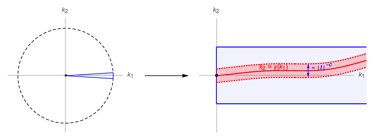
Figure 5.1. Frequency domain for $\mathbb{C}_{\mathbf{k}\approx\mathbf{K}_{\star}}(t;v,\theta)$

For the proof, we recall that changing the variable, the sectorial domain of integration for $\mathbb{C}_{\mathbf{k}\approx\mathbf{K}_{\star}}(t;v,\theta)$ is transformed into the rectangular one (see Figure 5.1). To refine the bound in the previous section, we find the curve $k_{2}=\gamma(k_{1})$ where the modified phase function $\tilde{\varphi}(\mathbf{k};v,\theta)$ is stationary in the $k_{2}$-direction at the frequency $\mathbf{k}=(k_{1},\gamma(k_{1}))$. Then, near the curve (the red region), we only consider the oscillation in the $k_{1}$-direction, but the additional decay is obtained from the small measure. On the other hand, away from the curve (the blue region), we take the additional decay by integration by parts in the $k_{2}$-direction. The $O(|t|^{-c})$-width of the red region will be chosen later to optimize the sum of the two bounds.

For this, using Lemma 5.11, we differentiate the phase in the $k_{2}$-direction and write

$$\partial_{k_{2}}\tilde{\varphi}(\mathbf{k};v,\theta)=\frac{\sqrt{3}k_{1}}{2}G(\mathbf{k}),$$ (5.12)

where

$$G(\mathbf{k}): =k_{2}+\bigg{(}-\frac{3b_{\theta}}{2}-\frac{7a_{\theta}}{2}k_{2}+\frac{15b_{\theta}}{4}k_{2}^{2}\bigg{)}k_{1}$$ (5.13)

$$\quad+\bigg{(}\frac{3a_{\theta}b_{\theta}}{4}+\frac{3(44a_{\theta}^{2}-3)}{32}k_{2}-\frac{87}{8}a_{\theta}b_{\theta}k_{2}^{2}\bigg{)}k_{1}^{2}+k_{1}^{3}\mathcal{O}_{0}(\mathbf{k})+k_{2}^{3}\tilde{\mathcal{O}}_{0}(\mathbf{k}).$$

By the implicit function theorem, we determine the frequencies where $G(\mathbf{k})$ vanishes, which is equivalent to $\partial_{k_{2}}\tilde{\varphi}(\mathbf{k};v,\theta)=0$ when $k_{1}>0$.

Lemma 5.14.

There exist small $\delta_{0}>0$ and an analytic curve $\gamma:(-\delta_{0},\delta_{0})\to\mathbb{R}$ such that if $|k_{1}|<\delta_{0}$, then $G(k_{1},\gamma(k_{1}))=0$ and

$$\gamma(k_{1})=\frac{3b_{\theta}}{2}k_{1}+\frac{9a_{\theta}b_{\theta}}{2}k_{1}^{2}+\mathcal{O}_{3}(k_{1}),$$

where $\mathcal{O}_{3}(k_{1})$ is an analytic function of $k_{1}$ near the origin such that $|\mathcal{O}_{3}(k_{1})|\lesssim|k_{1}|^{3}$ (see (2.16)).

Proof.

Note that $G(\mathbf{0})=0$ and $\partial_{k_{2}}G(\mathbf{k})\geq\frac{1}{2}$ near the origin, because

$$\partial_{k_{2}}G(\mathbf{k}) =1+\bigg{(}-\frac{7a_{\theta}}{2}+\frac{15b_{\theta}}{2}k_{2}\bigg{)}k_{1}+\bigg{(}\frac{3(44a_{\theta}^{2}-3)}{32}-\frac{87}{4}a_{\theta}b_{\theta}k_{2}\bigg{)}k_{1}^{2}$$ (5.14)

$$\quad+k_{1}^{3}\mathcal{O}_{0}(\mathbf{k})+k_{2}^{2}\tilde{\mathcal{O}}_{0}(\mathbf{k}).$$

Therefore, by the implicit function theorem, there exist small $\delta_{0}>0$ and $\gamma:(-\delta_{0},\delta_{0})\to\mathbb{R}$ such that $G(k_{1},\gamma(k_{1}))=0$ and $\gamma^{\prime}(k_{1})=-\frac{(\partial_{k_{1}}G)(k_{1},\gamma(k_{1}))}{(\partial_{k_{2}}G)(k_{1},\gamma(k_{1}))}$. Note that $|\gamma^{\prime}(k_{1})|\lesssim 1$, because $|\partial_{k_{1}}G(\mathbf{k})|\lesssim 1$ and $\partial_{k_{2}}G(\mathbf{k})\geq\frac{1}{2}$ near the origin. Subsequently, since $\partial_{k_{1}}G(\mathbf{k})$ is analytic and $\partial_{k_{2}}G(\mathbf{k})\geq\frac{1}{2}$, differentiating $\gamma^{\prime}(k_{1})=-\frac{(\partial_{k_{1}}G)(k_{1},\gamma(k_{1}))}{(\partial_{k_{2}}G)(k_{1},\gamma(k_{1}))}$, we obtain $|\gamma^{\prime\prime}(k_{1})|\lesssim 1$. Repeating one can show that $|\gamma^{(j)}(k_{1})|\lesssim_{j}1$ whose implicit constant grows at most polynomially. Hence, $\gamma(k_{1})$ is analytic near the origin. Subsequently, in principle, plugging the series expansion for $\gamma(k_{1})=\sum_{m=1}^{\infty}d_{m}k_{1}^{m}$ into the equation

$$0 =G(k_{1},\gamma(k_{1}))$$

$$=\gamma(k_{1})+\bigg{(}-\frac{3b_{\theta}}{2}-\frac{7a_{\theta}}{2}\gamma(k_{1})+\frac{15b_{\theta}}{4}\gamma(k_{1})^{2}\bigg{)}k_{1}$$

$$\quad+\bigg{(}\frac{3a_{\theta}b_{\theta}}{4}+\frac{3(44a_{\theta}^{2}-3)}{32}\gamma(k_{1})-\frac{87}{8}a_{\theta}b_{\theta}\gamma(k_{1})^{2}\bigg{)}k_{1}^{2}+k_{1}^{3}\mathcal{O}_{0}(\mathbf{k})+\gamma(k_{1})^{3}\tilde{\mathcal{O}}_{0}(\mathbf{k}),$$

one can determine the coefficients $d_{m}$. Indeed, collecting all cubic and higher-order terms in $\mathcal{O}_{3}(k_{1})$, the above equation can be written as

$$0 =d_{1}k_{1}+d_{2}k_{1}^{2}+\bigg{(}-\frac{3b_{\theta}}{2}-\frac{7a_{\theta}}{2}d_{1}k_{1}\bigg{)}k_{1}+\frac{3a_{\theta}b_{\theta}}{4}k_{1}^{2}+\mathcal{O}_{3}(k_{1})$$

$$=\bigg{(}d_{1}-\frac{3b_{\theta}}{2}\bigg{)}k_{1}+\bigg{(}d_{2}-\frac{7a_{\theta}}{2}d_{1}+\frac{3a_{\theta}b_{\theta}}{4}\bigg{)}k_{1}^{2}+\mathcal{O}_{3}(k_{1}).$$

Therefore, it follows that $d_{1}=\frac{3b_{\theta}}{2}$ and $d_{2}=\frac{9a_{\theta}b_{\theta}}{2}$. ∎

Next, truncating around the curve $k_{2}=\gamma(k_{1})$ (see Figure 5.1), we decompose

$$\mathbb{C}_{\mathbf{k}\approx\mathbf{K}_{\star}}(t;v,\theta) =\sum_{j=0,1}e^{i\mathbf{K}_{\star}\cdot\mathbf{v}}\int_{0}^{\infty}\int_{-\infty}^{\infty}e^{-it\tilde{\varphi}(\mathbf{k};v,\theta)}\tilde{\chi}_{\delta}(\mathbf{k})\chi_{j}\bigg{(}\frac{k_{2}-\gamma(k_{1})}{|t|^{-c}}\bigg{)}k_{1}dk_{2}dk_{1}$$ (5.15)

$$=:\sum_{j=0,1}\mathbb{C}^{j}_{\mathbf{k}\approx\mathbf{K}_{\star}}(t;v,\theta)$$

where $\chi_{0}$ and $\chi_{1}$ are given in (2.13) and (2.14) and $c>0$ will be chosen later. For $\mathbb{C}^{0}_{\mathbf{k}\approx\mathbf{K}_{\star}}(t;v,\theta)$, a decay bound is obtained only from the oscillation for the $k_{1}$-variable.

Lemma 5.15 (Bound for $\mathbb{C}^{0}_{\mathbf{k}\approx\mathbf{K}_{\star}}(t;v,\theta)$).

$$\sup_{v>0\textup{ and }\theta\in[0,2\pi)}|\mathbb{C}^{0}_{\mathbf{k}\approx\mathbf{K}_{\star}}(t;v,\theta)| \lesssim(1+|t|)^{-\frac{1}{3}-c},$$

$$\sup_{v>0\textup{ and }|\theta-\frac{\pi n}{3}|\geq\epsilon}|\mathbb{C}^{0}_{\mathbf{k}\approx\mathbf{K}_{\star}}(t;v,\theta)| \lesssim_{\epsilon}(1+|t|)^{-\frac{1}{2}-c}.$$

Proof.

We may assume that $|t|\geq 1$, since $\textup{C}_{\leq\delta,(0)}^{\textup{Dirac}}(t,v,\theta)$ is bounded. For the proof, by Fubini’s theorem, we write

$$\mathbb{C}^{0}_{\mathbf{k}\approx\mathbf{K}_{\star}}(t;v,\theta)=e^{i\mathbf{K}_{\star}\cdot\mathbf{v}}\int_{-\infty}^{\infty}\bigg{\{}\int_{0}^{\infty}e^{-it\tilde{\tilde{\varphi}}(\mathbf{k})}\tilde{\tilde{\chi}}_{\delta}(\mathbf{k})k_{1}dk_{1}\bigg{\}}\chi_{0}\bigg{(}\frac{k_{2}}{|t|^{-c}}\bigg{)}dk_{2},$$ (5.16)

where

$$\tilde{\tilde{\varphi}}(\mathbf{k}):=\tilde{\varphi}(k_{1},k_{2}+\gamma(k_{1});v,\theta)$$ (5.17)

and

$$\tilde{\tilde{\chi}}_{\delta}(\mathbf{k}):=\tilde{\chi}_{\delta}(k_{1},k_{2}+\gamma(k_{1})).$$ (5.18)

Note here that by Remark 5.10 and Lemma 5.14, $\tilde{\tilde{\chi}}_{\delta}$ is smooth and is supported in $[-20\delta,20\delta]^{2}$. For the phase function, plugging $(k_{1},k_{2}+\gamma(k_{1}))$ in Lemma 5.11, we obtain that

$$\tilde{\tilde{\varphi}}(\mathbf{k}) =\frac{\sqrt{3}k_{1}}{2}\bigg{\{}1-\frac{2}{\sqrt{3}}v+\frac{1}{2}(k_{2}+\gamma(k_{1}))^{2}$$

$$\qquad\qquad+\bigg{(}\frac{a_{\theta}}{2}-\frac{3b_{\theta}}{2}(k_{2}+\gamma(k_{1}))-\frac{7a_{\theta}}{4}(k_{2}+\gamma(k_{1}))^{2}+\frac{5b_{\theta}}{4}(k_{2}+\gamma(k_{1}))^{3}\bigg{)}k_{1}$$

$$\qquad\qquad+\bigg{(}-\frac{1}{32}-\frac{a_{\theta}^{2}}{8}+\frac{3a_{\theta}b_{\theta}}{4}(k_{2}+\gamma(k_{1}))+\frac{3(44a_{\theta}^{2}-3)}{64}(k_{2}+\gamma(k_{1}))^{2}$$

$$\qquad\qquad\qquad-\frac{29}{8}a_{\theta}b_{\theta}(k_{2}+\gamma(k_{1}))^{3}\bigg{)}k_{1}^{2}+(k_{1}^{3}+(k_{2}+\gamma(k_{1}))^{4})\mathcal{O}_{0}(k_{1},k_{2}+\gamma(k_{1}))\bigg{\}}.$$

In the parentheses $\{\cdots\}$, we insert $\gamma(k_{1})=\frac{3b_{\theta}}{2}k_{1}+\frac{9a_{\theta}b_{\theta}}{2}k_{1}^{2}+\mathcal{O}_{3}(k_{1})$ (see Lemma 5.14), and collect all higher-order terms in $\mathcal{O}_{3}(k_{1})+k_{2}^{2}\mathcal{O}_{0}(\mathbf{k})$. Then, it follows that

$$\tilde{\tilde{\varphi}}(\mathbf{k}) =\frac{\sqrt{3}k_{1}}{2}\bigg{\{}1-\frac{2}{\sqrt{3}}v+k_{2}\gamma(k_{1})+\frac{\gamma(k_{1})^{2}}{2}$$ (5.19)

$$\qquad\qquad+\bigg{(}\frac{a_{\theta}}{2}-\frac{3b_{\theta}}{2}(k_{2}+\gamma(k_{1}))-\frac{7a_{\theta}}{2}k_{2}\gamma(k_{1})\bigg{)}k_{1}$$

$$\qquad\qquad+\bigg{(}-\frac{1}{32}-\frac{a_{\theta}^{2}}{8}+\frac{3a_{\theta}b_{\theta}}{4}k_{2}\bigg{)}k_{1}^{2}+O_{3}(k_{1})+k_{2}^{2}\mathcal{O}_{0}(\mathbf{k})\bigg{\}}$$

$$=\frac{\sqrt{3}k_{1}}{2}\bigg{\{}1-\frac{2}{\sqrt{3}}v+\frac{a_{\theta}}{2}k_{1}-\bigg{(}\frac{1}{8}-a_{\theta}^{2}\bigg{)}k_{1}^{2}+\mathcal{O}_{3}(k_{1})+k_{2}^{2}\mathcal{O}_{0}(\mathbf{k})\bigg{\}}$$

$$=\bigg{(}\frac{\sqrt{3}}{2}-v\bigg{)}k_{1}+\frac{\sqrt{3}a_{\theta}}{4}k_{1}^{2}-\frac{\sqrt{3}}{2}\bigg{(}\frac{1}{8}-a_{\theta}^{2}\bigg{)}k_{1}^{3}+k_{1}\mathcal{O}_{3}(k_{1})+k_{1}k_{2}^{2}\mathcal{O}_{0}(\mathbf{k}),$$

where (5.5) is used to remove $b_{\theta}$ in the last step. Note from (5.19) that if $k_{1}>0$ is small enough, then

$$|\partial_{k_{1}}^{2}\tilde{\tilde{\varphi}}(\mathbf{k})|=\bigg{|}\frac{\sqrt{3}a_{\theta}}{2}-3\sqrt{3}\bigg{(}\frac{1}{8}-a_{\theta}^{2}\bigg{)}k_{1}+\mathcal{O}_{2}(\mathbf{k})\bigg{|}\sim 1,$$ (5.20)

provided that $|a_{\theta}|\gtrsim 1$. Moreover, for any $\theta\in[0,2\pi)$, we have

$$|\partial_{k_{1}}^{3}\tilde{\tilde{\varphi}}(\mathbf{k})|=\bigg{|}-3\sqrt{3}\bigg{(}\frac{1}{8}-a_{\theta}^{2}\bigg{)}+\mathcal{O}_{1}(\mathbf{k})\bigg{|}\sim 1,$$ (5.21)

since $a_{\theta}^{2}\leq\frac{1}{12}$ (see (5.5)). Hence, applying the van der Corput lemma [58] to the inner integral (5.16), we obtain

$$\bigg{|}\int_{0}^{\infty}e^{-it\tilde{\tilde{\varphi}}(\mathbf{k})}\tilde{\tilde{\chi}}_{\delta}(\mathbf{k})k_{1}dk_{1}\bigg{|}\lesssim\left\{\begin{aligned} &|t|^{-\frac{1}{2}}&&\textup{if }|a_{\theta}|\gtrsim 1\\ &|t|^{-\frac{1}{3}}&&\textup{otherwise}.\end{aligned}\right.$$

Therefore, applying this bound to the inner integral in (5.16) with $|k_{2}|\lesssim|t|^{-c}$, we prove the lemma. ∎

In the integral $\mathbb{C}^{1}_{\mathbf{k}\approx\mathbf{K}_{\star}}(t;v,\theta)$, the frequencies such that $\partial_{k_{2}}\tilde{\varphi}(\mathbf{k};v,\theta)$ is small are truncated out. Thus, the additional decay is obtained by integration by parts for the $k_{2}$-variable as in the proof of the preliminary bound (Proposition 5.8), but we also capture the oscillation in the $k_{1}$-direction.

Lemma 5.16 (Bound for $\mathbb{C}^{1}_{\mathbf{k}\approx\mathbf{K}_{\star}}(t;v,\theta)$).

$$\sup_{v>0\textup{ and }\theta\in[0,2\pi)}|\mathbb{C}^{1}_{\mathbf{k}\approx\mathbf{K}_{\star}}(t;v,\theta)| \lesssim(1+|t|)^{-(\frac{4}{3}-c)},$$

$$\sup_{v>0\textup{ and }|\theta-\frac{\pi n}{3}|\geq\epsilon}|\mathbb{C}^{1}_{\mathbf{k}\approx\mathbf{K}_{\star}}(t;v,\theta)| \lesssim_{\epsilon}(1+|t|)^{-(\frac{3}{2}-c)}.$$

Proof.

Again, we may assume that $|t|\geq 1$. By integration by parts with $\partial_{k_{2}}\tilde{\varphi}(\mathbf{k};v,\theta)=\frac{\sqrt{3}k_{1}}{2}G(\mathbf{k})$ (see (5.12)) and distributing the derivative, $\mathbb{C}^{1}_{\mathbf{k}\approx\mathbf{K}_{\star}}(t;v,\theta)$ can be written as

$$\mathbb{C}^{1}_{\mathbf{k}\approx\mathbf{K}_{\star}}(t;v,\theta) =-\frac{e^{i\mathbf{K}_{\star}\cdot\mathbf{v}}}{it}\int_{0}^{\infty}\int_{-\infty}^{\infty}\partial_{k_{2}}(e^{-it\tilde{\varphi}(\mathbf{k};v,\theta)})\Bigg{\{}\frac{\tilde{\chi}_{\delta}(\mathbf{k})\chi_{1}(\frac{k_{2}-\gamma(k_{1})}{|t|^{-c}})}{\frac{\sqrt{3}k_{1}}{2}G(\mathbf{k})}\Bigg{\}}k_{1}dk_{2}dk_{1}$$

$$=\frac{2e^{i\mathbf{K}_{\star}\cdot\mathbf{v}}}{i\sqrt{3}t}\int_{0}^{\infty}\int_{-\infty}^{\infty}e^{-it\tilde{\varphi}(\mathbf{k};v,\theta)}\partial_{k_{2}}\Bigg{\{}\frac{\tilde{\chi}_{\delta}(\mathbf{k})\chi_{1}(\frac{k_{2}-\gamma(k_{1})}{|t|^{-c}})}{G(\mathbf{k})}\Bigg{\}}dk_{2}dk_{1}$$

$$=\frac{2e^{i\mathbf{K}_{\star}\cdot\mathbf{v}}}{i\sqrt{3}t}\int_{-\infty}^{\infty}\Bigg{[}\int_{0}^{\infty}e^{-it\tilde{\tilde{\varphi}}(\mathbf{k};v,\theta)}\partial_{k_{2}}\Bigg{\{}\frac{\tilde{\tilde{\chi}}_{\delta}(\mathbf{k})\chi_{1}(\frac{k_{2}}{|t|^{-c}})}{G(k_{1},\gamma(k_{1})+k_{2})}\Bigg{\}}dk_{1}\Bigg{]}dk_{2},$$

where $\tilde{\tilde{\varphi}}(\mathbf{k})$ and $\tilde{\tilde{\chi}}_{\delta}(\mathbf{k})$ are defined in (5.17) and (5.18). Hence, using the lower bounds for the second and the third derivatives of $\tilde{\varphi}(k_{1},k_{2}+\gamma(k_{1}))$ depending on $\theta$ (see (5.20) and (5.21)) and employing the van der Corput lemma [58] for the inner $k_{1}$-integral as in the proof of Lemma 5.15, we obtain

$$|\mathbb{C}^{1}_{\mathbf{k}\approx\mathbf{K}_{\star}}(t;v,\theta)|\lesssim\left\{\begin{aligned} &\mathcal{R}(t)|t|^{-\frac{3}{2}}&&\textup{if }|\theta-\tfrac{\pi n}{3}|\geq\epsilon\\ &\mathcal{R}(t)|t|^{-\frac{4}{3}}&&\textup{otherwise},\end{aligned}\right.$$

where

$$\mathcal{R}(t):=\int_{-\infty}^{\infty}\int_{0}^{\infty}\bigg{|}\partial_{k_{1}}\partial_{k_{2}}\bigg{\{}\frac{\tilde{\tilde{\chi}}_{\delta}(\mathbf{k})\chi_{1}(\frac{k_{2}}{|t|^{-c}})}{G(k_{1},\gamma(k_{1})+k_{2})}\bigg{\}}\bigg{|}dk_{1}dk_{2}.$$

Therefore, it is enough to show that

$$\mathcal{R}(t)\lesssim|t|^{c}.$$ (5.22)

Indeed, we observe that $\tilde{\tilde{\chi}}_{\delta}(\mathbf{k})$ is smooth and is supported in the area $[-3\delta,3\delta]^{2}$. Thus, it follows that

$$|\mathcal{R}(t)| \lesssim\int_{-3\delta}^{3\delta}\int_{0}^{3\delta}\bigg{|}\frac{\chi_{1}(\frac{k_{2}}{|t|^{-c}})}{G(k_{1},\gamma(k_{1})+k_{2})}\bigg{|}+\bigg{|}\nabla_{\mathbf{k}}\bigg{(}\frac{\chi_{1}(\frac{k_{2}}{|t|^{-c}})}{G(k_{1},\gamma(k_{1})+k_{2})}\bigg{)}\bigg{|}$$

$$\qquad\qquad\qquad\qquad\qquad\qquad\quad\ \ +\bigg{|}\partial_{k_{1}}\partial_{k_{2}}\bigg{(}\frac{\chi_{1}(\frac{k_{2}}{|t|^{-c}})}{G(k_{1},\gamma(k_{1})+k_{2})}\bigg{)}\bigg{|}dk_{1}dk_{2}.$$

Note that by the fact that

$$\partial_{k_{2}}G(\mathbf{k})\sim 1$$ (5.23)

(see (5.14)), the fundamental theorem of calculus with $G(k_{1},\gamma(k_{1}))=0$ yields

$$\big{|}G(k_{1},\gamma(k_{1})+k_{2})\big{|}=\bigg{|}\int_{0}^{k_{2}}\partial_{k_{2}}G(k_{1},\gamma(k_{1})+s)ds\bigg{|}\sim|k_{2}|.$$ (5.24)

Moreover, repeating the calculations in (5.19) (see (5.12) for the definition of $G(\mathbf{k})$), one can show that

$$\partial_{k_{1}}\big{(}G(k_{1},\gamma(k_{1})+k_{2})\big{)}$$ (5.25)

$$=\partial_{k_{1}}\partial_{k_{2}}\bigg{\{}1-\frac{2}{\sqrt{3}}v+\frac{a_{\theta}}{2}k_{1}-\bigg{(}\frac{1}{8}-a_{\theta}^{2}\bigg{)}k_{1}^{2}+\mathcal{O}_{3}(k_{1})+k_{2}^{2}\mathcal{O}_{0}(\mathbf{k})\bigg{\}}=k_{2}\mathcal{O}_{0}(\mathbf{k})$$

and

$$\partial_{k_{1}}\partial_{k_{2}}\big{(}G(k_{1},\gamma(k_{1})+k_{2})\big{)}=\mathcal{O}_{0}(\mathbf{k}).$$ (5.26)

Therefore, by (5.23), (5.24) and (5.25), we have

$$\bigg{|}\frac{\chi_{1}(\frac{k_{2}}{|t|^{-c}})}{G(k_{1},\gamma(k_{1})+k_{2})}\bigg{|}+\bigg{|}\nabla_{\mathbf{k}}\bigg{(}\frac{\chi_{1}(\frac{k_{2}}{|t|^{-c}})}{G(k_{1},\gamma(k_{1})+k_{2})}\bigg{)}\bigg{|}$$

$$\leq\chi_{1}\bigg{(}\frac{k_{2}}{|t|^{-c}}\bigg{)}\bigg{\{}\frac{1}{|G(k_{1},\gamma(k_{1})+k_{2})|}+\frac{|\nabla_{\mathbf{k}}(G(k_{1},\gamma(k_{1})+k_{2}))|}{G(k_{1},\gamma(k_{1})+k_{2})^{2}}\bigg{\}}+\frac{|\frac{1}{|t|^{-c}}\chi_{0}^{\prime}(\frac{k_{2}}{|t|^{-c}})|}{G(k_{1},\gamma(k_{1})+k_{2})}$$

$$\lesssim\frac{\chi_{1}(\frac{k_{2}}{|t|^{-c}})}{|k_{2}|}+\frac{\chi_{1}(\frac{k_{2}}{|t|^{-c}})}{k_{2}^{2}}+\frac{|\frac{1}{|t|^{-c}}\chi_{0}^{\prime}(\frac{k_{2}}{|t|^{-c}})|}{|k_{2}|}\lesssim|t|^{c}+\frac{\mathbbm{1}_{|k_{2}|\gtrsim|t|^{-c}}}{k_{2}^{2}}+|t|^{2c}\mathbbm{1}_{|k_{2}|\sim|t|^{-c}}.$$

On the other hand, applying (5.23), (5.24), (5.25) and (5.26) to

$$\partial_{k_{1}}\partial_{k_{2}}\bigg{(}\frac{\chi_{1}(\frac{k_{2}}{|t|^{-c}})}{G(k_{1},\gamma(k_{1})+k_{2})}\bigg{)} =\chi_{1}\bigg{(}\frac{k_{2}}{|t|^{-c}}\bigg{)}\bigg{\{}-\frac{\partial_{k_{1}}\partial_{k_{2}}(G(k_{1},\gamma(k_{1})+k_{2}))}{G(k_{1},\gamma(k_{1})+k_{2})^{2}}$$

$$\qquad\qquad\qquad+\frac{\partial_{k_{1}}(G(k_{1},\gamma(k_{1})+k_{2}))\partial_{k_{2}}(G(k_{1},\gamma(k_{1})+k_{2}))}{G(k_{1},\gamma(k_{1})+k_{2})^{3}}\bigg{\}}$$

$$\quad-\frac{\partial_{k_{1}}(G(k_{1},\gamma(k_{1})+k_{2}))\frac{1}{|t|^{-c}}\chi_{0}^{\prime}(\frac{k_{2}}{|t|^{-c}})}{G(k_{1},\gamma(k_{1})+k_{2})^{2}},$$

we obtain that

$$\bigg{|}\partial_{k_{1}}\partial_{k_{2}}\bigg{(}\frac{\chi_{1}(\frac{k_{2}}{|t|^{-c}})}{G(k_{1},\gamma(k_{1})+k_{2})}\bigg{)}\bigg{|}\lesssim\frac{\mathbbm{1}_{|k_{2}|\gtrsim|t|^{-c}}}{k_{2}^{2}}+|t|^{2c}\mathbbm{1}_{|k_{2}|\sim|t|^{-c}},$$

where for the second upper bound, we used that $\partial_{k_{2}}G(\mathbf{k})>0$ (see (5.23)). Therefore, collecting all, we prove that

$$|\mathcal{R}(t)|\lesssim\int_{-3\delta}^{3\delta}\int_{0}^{3\delta}\bigg{\{}|t|^{c}+\frac{\mathbbm{1}_{|k_{2}|\gtrsim|t|^{-c}}}{k_{2}^{2}}+|t|^{2c}\mathbbm{1}_{|k_{2}|\sim|t|^{-c}}\bigg{\}}dk_{2}dk_{1}\sim|t|^{c},$$

where in the last step, we used that by the mean value theorem, $G(k_{1},\gamma(k_{1})\pm C|t|^{-c})=G(k_{1},\gamma(k_{1}))\pm\partial_{k_{2}}G(k_{1},k_{2}^{*})C|t|^{-c}\sim\pm|t|^{-c}$ as well as $G(k_{1},\gamma(k_{1}))=0$ and $\partial_{k_{2}}G(\mathbf{k})\sim 1$. This completes the proof of (5.22). ∎

Finally, we are ready to prove the main result of this section.

Proof of Proposition 5.12.

We apply Lemma 5.15 and 5.16 to the decomposition (5.15). Then, choosing $c>0$ optimizing the bound, we prove Proposition 5.12. ∎

6. Oscillatory integral localized at a Dirac point at an intersection of two degenerate frequency curves

Next, we show Theorem 4.1 for $\mathbf{K}_{2}\in\mathcal{K}_{2}^{\prime}$, that is, one of the intersections of two degenerate frequency curves (see Figure 2.1).

Theorem 6.1 (Oscillatory integral estimate; $\mathbf{K}=\mathbf{K}_{2}$).

For $\mathbf{K}_{2}=(0,\pi)$, there exist $C_{2}>0$ and a smooth cut-off $\chi_{\leq\delta}$, whose support is contained in a sufficiently small disk of radius $\delta>0$, such that for any $\mathbf{v}\in\mathbb{R}^{2}$,

$$|\mathbb{I}_{\mathbf{k}\approx\mathbf{K}_{2}}(t;\mathbf{v})|\leq\frac{C_{2}}{(1+|t|)^{2/3}}.$$

Remark 6.2.

By the reduction in Section 4, Theorem 6.1 implies Theorem 4.1 for $\mathbf{K}\in\mathcal{K}_{2}$.

6.1. Reduction to the degenerate oscillatory integral

For the oscillatory integral

$$\mathbb{I}_{\mathbf{k}\approx\mathbf{K}_{2}}(t;\mathbf{v}):=e^{it\mathbf{K}_{2}\cdot\mathbf{v}}\int_{-\infty}^{\infty}\int_{-\infty}^{\infty}e^{-it(\varphi(\mathbf{K}_{2}+\mathbf{k})-\mathbf{k}\cdot\mathbf{v})}\chi_{\leq\delta}(\mathbf{k})d\mathbf{k},$$

we change the variables by $\tilde{\mathbf{k}}=(\mathbf{k}\cdot\mathbf{v}_{1},\mathbf{k}\cdot\mathbf{v}_{2})$ with $\mathbf{v}_{1}=(\frac{\sqrt{3}}{2},\frac{1}{2})$ and $\mathbf{v}_{2}=(\frac{\sqrt{3}}{2},-\frac{1}{2})$. Then, it is important to observe from direct calculations for the phase formula (2.1) with the expansion $\sqrt{1+x}=1+\frac{1}{2}x-\frac{1}{8}x^{2}+\frac{1}{16}x^{3}+\cdots$ that in the new coordinates, the phase function is expanded as

$$\varphi(\mathbf{K}_{2}+\mathbf{k}) =\sqrt{3-2\sin(\mathbf{k}\cdot\mathbf{v}_{1})+2\sin(\mathbf{k}\cdot\mathbf{v}_{2})-2\cos(\mathbf{k}\cdot(\mathbf{v}_{1}-\mathbf{v}_{2}))}$$

$$=\sqrt{3-2\sin\tilde{k}_{1}+2\sin\tilde{k}_{2}-2\cos(\tilde{k}_{1}-\tilde{k}_{2})}$$

$$=\bigg{\{}1-2(\tilde{k}_{1}-\tilde{k}_{2})+(\tilde{k}_{1}-\tilde{k}_{2})^{2}+\frac{(\tilde{k}_{1})^{3}-(\tilde{k}_{2})^{3}}{3}+\mathcal{O}_{4}(\tilde{\mathbf{k}})\bigg{\}}^{\frac{1}{2}}$$

$$=1-\tilde{k}_{1}+\tilde{k}_{2}+\frac{1}{6}(\tilde{k}_{1})^{3}-\frac{1}{6}(\tilde{k}_{2})^{3}+\mathcal{O}_{4}(\tilde{\mathbf{k}}),$$

where $\mathcal{O}_{4}(\tilde{\mathbf{k}})$ is an analytic function such that $|\mathcal{O}_{4}(\tilde{\mathbf{k}})|\lesssim|\mathbf{k}|^{4}$ (see (2.16)). Subsequently, the integral becomes

$$\mathbb{I}_{\mathbf{k}\approx\mathbf{K}_{2}}(t;\mathbf{v})=\frac{2}{\sqrt{3}}e^{it(\mathbf{K}_{2}\cdot\mathbf{v}-1)}\int_{-\infty}^{\infty}\int_{-\infty}^{\infty}e^{-it(\frac{1}{6}(\tilde{k}_{1})^{3}-\frac{1}{6}(\tilde{k}_{2})^{3}+\mathcal{O}_{4}(\tilde{\mathbf{k}})-\tilde{v}_{1}\tilde{k}_{1}-\tilde{v}_{2}\tilde{k}_{2})}\chi_{0}\bigg{(}\frac{|\tilde{\mathbf{k}}|}{\delta}\bigg{)}d\tilde{\mathbf{k}},$$ (6.1)

where $(\tilde{v}_{1},\tilde{v}_{2})=(1+\frac{1}{\sqrt{3}}v_{1}+v_{2},-1+\frac{1}{\sqrt{3}}v_{1}-v_{2})$, and the cut-off $\chi_{\leq\delta}$ is chosen so that $\chi_{\leq\delta}(\frac{\tilde{k}_{1}+\tilde{k}_{2}}{\sqrt{3}},\tilde{k}_{1}-\tilde{k}_{2})=\chi_{0}(\frac{|\tilde{\mathbf{k}}|}{\delta})$.

Now, generalizing the right hand side of (6.1) up to trivial changes of variables, we define the oscillatory integral

$$\mathbb{I}_{2}(t;\mathbf{v}):=\int_{-\infty}^{\infty}\int_{-\infty}^{\infty}e^{-it(\phi_{2}(\mathbf{k})-\mathbf{k}\cdot\mathbf{v})}\chi_{0}\bigg{(}\frac{|\mathbf{k}|}{\delta_{0}\delta}\bigg{)}d\mathbf{k},$$

where $0<\delta\ll\delta_{0}\ll 1$ and $\chi_{0}(\frac{\cdot}{\delta_{0}\delta})=\sum_{N\leq\delta}\eta(\frac{\cdot}{\delta_{0}N})$ and

$$\phi_{2}(\mathbf{k}):=\pm k_{1}^{3}+k_{2}^{3}+\mathcal{O}_{4}(\mathbf{k}).$$

Remark 6.3.

For numerical simplicity in the proof below, the smooth cut-off $\chi_{0}(\frac{|\cdot|}{\delta})$ in $\mathbb{I}_{\mathbf{k}\approx\mathbf{K}_{2}}(t;\mathbf{v})$ replaced by $\chi_{0}(\frac{|\cdot|}{\delta_{0}\delta})$ in $\mathbb{I}_{2}(t;\mathbf{v})$. Indeed, this change does not affect the result, because small $\delta>0$ is not specified in Theorem 6.1.

Subsequently, the proof of Theorem 6.1 is reduced to the following proposition.

Proposition 6.4.

$$\sup_{\mathbf{v}\in\mathbb{R}^{2}}|\mathbb{I}_{2}(t;\mathbf{v})|\lesssim(1+|t|)^{-\frac{2}{3}}.$$

Remark 6.5.

By reduction, one can associate the phase $\phi_{2}(\mathbf{k}):=\pm k_{1}^{3}+k_{2}^{3}+\mathcal{O}_{4}(\mathbf{k})$ with a Newton polygon in Varchenko’s theorem [63]. Then, Proposition 6.4 follows together with Karpushkin’s stability theorem [41, 42].

6.2. Direct proof of Proposition 6.4

By the dyadic decomposition and rescaling, we decompose

$$\mathbb{I}_{2}(t;\mathbf{v})=\sum_{N\leq\delta}\int_{-\infty}^{\infty}\int_{-\infty}^{\infty}e^{-it(\phi_{2}(\mathbf{k})-\mathbf{k}\cdot\mathbf{v})}\eta\bigg{(}\frac{|\mathbf{k}|}{\delta_{0}N}\bigg{)}d\mathbf{k}=\sum_{N\leq\delta}N^{2}\mathbb{I}_{2;N}\bigg{(}N^{3}t;\frac{\mathbf{v}}{N^{2}}\bigg{)},$$

where $N=2^{m}\in 2^{\mathbb{Z}}$ denotes a dyadic number, $\eta$ is chosen in (2.15) and

$$\mathbb{I}_{2;N}(t;\mathbf{v}):=\int_{-\infty}^{\infty}\int_{-\infty}^{\infty}e^{-it(\phi_{2;N}(\mathbf{k})-\mathbf{k}\cdot\mathbf{v})}\eta\bigg{(}\frac{|\mathbf{k}|}{\delta_{0}}\bigg{)}d\mathbf{k}$$

with the phase

$$\phi_{2;N}(\mathbf{k}):=\frac{1}{N^{3}}\phi_{2}(N\mathbf{k})=\pm k_{1}^{3}+k_{2}^{3}+\frac{1}{N^{3}}\mathcal{O}_{4}(N\mathbf{k}).$$ (6.2)

In a sequel, we assume that $N\leq\delta$. Then, it is enough to show that

$$\sup_{\mathbf{v}\in\mathbb{R}^{2}}|\mathbb{I}_{2;N}(t;\mathbf{v})|\lesssim|t|^{-a}$$ (6.3)

for some $a>\frac{2}{3}$, because together with the trivial bound $|\mathbb{I}_{2;N}(t;\mathbf{v})|\lesssim 1$, (6.3) implies that $|\mathbb{I}_{2}(t;\mathbf{v})|\lesssim\sum_{N\leq\delta}N^{2}\min\{1,(N^{3}|t|)^{-a}\}\lesssim|t|^{-\frac{2}{3}}$. Indeed, for each $\mathbb{I}_{2;N}(t;\mathbf{v})$, we observe that for the contribution of the integral away from the $k_{1}$- and the $k_{2}$-axes, given by

$$\mathbb{I}_{2;N}^{\textup{away}}(t;\mathbf{v}):=\int_{-\infty}^{\infty}\int_{-\infty}^{\infty}e^{-it(\phi_{2;N}(\mathbf{k})-\mathbf{k}\cdot\mathbf{v})}\eta\bigg{(}\frac{|\mathbf{k}|}{\delta_{0}}\bigg{)}\bigg{\{}1-\chi_{0}\bigg{(}\frac{k_{2}}{\delta|k_{1}|}\bigg{)}-\chi_{0}\bigg{(}\frac{k_{1}}{\delta|k_{2}|}\bigg{)}\bigg{\}}d\mathbf{k},$$

the phase function satisfies $|\textup{det}(\nabla^{2}\phi_{2;N}(\mathbf{k}))|\sim|k_{1}||k_{2}|\sim_{\delta,\delta_{0}}1$ (see (6.2)). Thus, the standard non-degenerate phase oscillatory integral estimate immediately yields $|\mathbb{I}_{2;N}^{\textup{away}}(t;\mathbf{v})|\lesssim_{\delta,\delta_{0}}|t|^{-1}$. For (6.3), by symmetry, it remains to consider the contribution near the $k_{1}$-axis. Moreover, changing the variable $k_{1}$ by $-k_{1}$ for $k_{1}<0$ and by symmetry, it is enough to consider the integral near the positive part of the $k_{1}$-axis, that is,

$$\mathbb{I}_{2;N}^{\textup{near}}(t;\mathbf{v}):=\int_{-\infty}^{\infty}\int_{0}^{\infty}e^{-it(\phi_{2;N}(\mathbf{k})-\mathbf{k}\cdot\mathbf{v})}\eta\bigg{(}\frac{|\mathbf{k}|}{\delta_{0}}\bigg{)}\chi_{0}\bigg{(}\frac{k_{2}}{\delta k_{1}}\bigg{)}dk_{1}dk_{2}.$$

Therefore, the proof of (6.3) can be reduced to show that there exists $a>\frac{2}{3}$ such that

$$\sup_{\mathbf{v}\in\mathbb{R}^{2}}|\mathbb{I}_{2;N}^{\textup{near}}(t;\mathbf{v})|\lesssim|t|^{-a}.$$ (6.4)

To analyze the integral $\mathbb{I}_{2;N}^{\textup{near}}(t;\mathbf{v})$, we note that $|k_{1}|\sim|\mathbf{k}|\sim\delta_{0}$ and $|k_{2}|\lesssim\delta|k_{1}|\sim\delta_{0}\delta$ in the support of $\eta(\frac{|\mathbf{k}|}{\delta_{0}})\chi_{0}(\frac{k_{2}}{\delta k_{1}})$. Then, replacing $k_{1}$ by $k_{1}\mp k_{2}$ to cancel the cubic term $k_{2}^{3}$ in (6.2), we write

$$\mathbb{I}_{2;N}^{\textup{near}}(t;\mathbf{v}):=\int_{-\infty}^{\infty}\int_{0}^{\infty}e^{-it\tilde{\phi}_{2;N}(\mathbf{k};\mathbf{v})}\tilde{\chi}(\mathbf{k})dk_{1}dk_{2},$$

where

$$\tilde{\phi}_{2;N}(\mathbf{k};\mathbf{v}): =\pm k_{1}^{3}-3k_{1}^{2}k_{2}\pm 3k_{1}k_{2}^{2}+\frac{1}{N^{3}}\mathcal{O}_{4}(N\mathbf{k})-v_{1}k_{1}-(v_{2}\mp v_{1})k_{2}$$ (6.5)

and $\tilde{\chi}(\mathbf{k}):=\eta(\frac{|(k_{1}\mp k_{2},k_{2})|}{\delta_{0}})\chi_{0}(\frac{k_{2}}{\delta(k_{1}\mp k_{2})})$ is a smooth function supported in

$$k_{1}\sim\delta_{0}\quad\textup{and}\quad|k_{2}|\lesssim\delta_{0}\delta.$$ (6.6)

We observe that

$$\partial_{k_{2}}\tilde{\phi}_{2;N}(\mathbf{k};\mathbf{v})=\delta_{0}G_{N}(\mathbf{k})-3k_{1}^{2}-(v_{2}\mp v_{1}),$$ (6.7)

where

$$G_{N}(\mathbf{k}):=\frac{1}{\delta_{0}}\bigg{(}\pm 6k_{1}k_{2}+\frac{1}{N^{2}}\mathcal{O}_{3}(N\mathbf{k})\bigg{)}.$$ (6.8)

Since $|G_{N}(\mathbf{k})|\lesssim\delta_{0}\delta$ when $N\leq\delta$, it is natural to decompose further as

$$\mathbb{I}_{2;N}^{\textup{near}}(t;\mathbf{v})=\mathbb{I}_{2;N;(0)}^{\textup{near}}(t;\mathbf{v})+\mathbb{I}_{2;N;(1)}^{\textup{near}}(t;\mathbf{v}),$$

where

$$\mathbb{I}_{2;N;(j)}^{\textup{near}}(t;\mathbf{v}):=\int_{-\infty}^{\infty}\int_{0}^{\infty}e^{-it\tilde{\phi}_{2;N}(\mathbf{k};\mathbf{v})}\chi_{j}\bigg{(}\frac{3k_{1}^{2}+(v_{2}\mp v_{1})}{\delta_{0}\delta}\bigg{)}\tilde{\chi}(\mathbf{k})dk_{1}dk_{2}$$

(see (2.13) and (2.14) for the definition of $\chi_{0}$ and $\chi_{1}$). In the integral $\mathbb{I}_{2;N;(1)}^{\textup{near}}(t;\mathbf{v})$, we have $|\partial_{k_{2}}\tilde{\phi}_{2;N}(\cdot;\mathbf{v})|\geq|3k_{1}^{2}+(v_{2}\mp v_{1})|-\delta_{0}|G_{N}(\mathbf{k})|\gtrsim\delta_{0}\delta$. Hence, one can show that $|\mathbb{I}_{2;N;(1)}^{\textup{near}}(t;\mathbf{v})|\lesssim_{\delta_{0},\delta}|t|^{-1}$ by integration by parts for the $k_{2}$-variable.

It remains to consider $\mathbb{I}_{2;N;(0)}^{\textup{near}}(t;\mathbf{v})$. We will show that

$$|\mathbb{I}_{2;N;(0)}^{\textup{near}}(t;\mathbf{v})|\lesssim|t|^{-\frac{5}{6}},$$ (6.9)

which completes the proof of Proposition 6.4 (see (6.4)). Indeed, as we did in the proof of Lemma 5.14, we will prove (6.9) constructing the curve $k_{2}=\tilde{\gamma}_{N}(k_{1})$ such that $\tilde{\phi}_{2;N}(k_{1},\cdot;\mathbf{v})$ is stationary in the $k_{2}$-direction. Suppose that $\mathbf{k}$ is contained in the support of $\tilde{\chi}$ so that (6.6) holds. Then, by the definition (6.8), we have

$$\left\{\begin{aligned} G_{N}(\mathbf{0})&=0,\\ \partial_{k_{1}}G_{N}(\mathbf{k})&=\frac{1}{\delta_{0}}\bigg{(}\pm 6k_{2}+\frac{1}{N}\mathcal{O}_{2}(N\mathbf{k})\bigg{)},\\ \partial_{k_{2}}G_{N}(\mathbf{k})&=\frac{1}{\delta_{0}}\bigg{(}\pm 6k_{1}+\frac{1}{N}\mathcal{O}_{2}(N\mathbf{k})\bigg{)}\approx\pm\frac{6k_{1}}{\delta_{0}},\\ \partial_{k_{1}}^{j_{1}}\partial_{k_{2}}^{j_{2}}G_{N}(\mathbf{k})&=\frac{1}{\delta_{0}}N^{j_{1}+j_{2}-2}\mathcal{O}_{0}(N\mathbf{k})\quad\textup{for }j_{1}+j_{2}\geq 3,\end{aligned}\right.$$ (6.10)

where $N\leq\delta$. Hence, by the implicit function theorem together with $|\partial_{k_{2}}G_{N}(\mathbf{k})|\sim 1$ and (6.6), there exists a differentiable function $k_{2}=\gamma_{N}(k_{1})$ near the origin such that $G_{N}(k_{1},\gamma_{N}(k_{1}))=0$, $\gamma_{N}^{\prime}(k_{1})=-\frac{(\partial_{k_{1}}G_{N})(k_{1},\gamma_{N}(k_{1}))}{(\partial_{k_{2}}G_{N})(k_{1},\gamma_{N}(k_{1}))}$, $|\gamma_{N}(k_{1})|\lesssim\delta_{0}\delta$ and $|\gamma_{N}^{\prime}(k_{1})|\lesssim\delta$. Moreover, since differentiation of $G_{N}(\mathbf{k})$ generates only polynomially many terms with geometrically decreasing higher-order derivatives (see the last line of (6.10)), it follows that $\gamma_{N}(k_{1})$ is analytic near the origin.

Next, we claim that more than analyticity, $\gamma_{N}(k_{1})$ is of the form

$$\gamma_{N}(k_{1})=\frac{(Nk_{1})^{2}}{N}\mathcal{O}_{0}(Nk_{1}).$$ (6.11)

For the proof, we insert $k_{2}=\gamma_{N}(k_{1})=\frac{(Nk_{1})^{2}}{N}g(Nk_{1})$ for some unknown function $g$ in (6.8) with $\mathcal{O}_{3}(\mathbf{k})=\sum_{m_{1}+m_{2}\geq 3}c_{m_{1},m_{2}}k_{1}^{m_{1}}k_{2}^{m_{2}}$. Then, we obtain

$$G_{N}(k_{1},\gamma_{N}(k_{1}))=\frac{Nk_{1}^{3}}{\delta_{0}}H_{N}(Nk_{1},g(Nk_{1}))=0,$$

where

$$H_{N}(\mathbf{k})=\pm 6k_{2}+\sum_{m_{1}+m_{2}\geq 3}c_{m_{1},m_{2}}k_{1}^{m_{1}+2m_{2}-3}k_{2}^{m_{2}}=\pm 6k_{2}+\mathcal{O}_{0}(\mathbf{k}).$$

Hence, applying the implicit function theorem to $H_{N}(\mathbf{k})=0$ with $\partial_{k_{2}}H_{N}(\mathbf{k})\approx\pm 6$ as we did to construct $\gamma_{N}$, we can construct an analytic function $g(k_{1})$ near the origin. This proves the claim (6.11).

Subsequently, for each $k_{1}\sim\delta_{0}$, expanding the Taylor series around $k_{2}=\gamma_{N}(k_{1})$ with $G_{N}(k_{1},\gamma_{N}(k_{1}))=0$, the equation $\partial_{k_{2}}\tilde{\phi}_{2;N}(k_{1},\cdot;\mathbf{v})=0$ (see (6.7)) can be written as

$$0=-\frac{3k_{1}^{2}+(v_{2}\mp v_{1})}{\delta_{0}}+\sum_{m=1}^{\infty}\frac{\partial_{k_{2}}^{m}G_{N}(k_{1},\gamma_{N}(k_{1}))}{m!}(\cdot-\gamma_{N}(k_{1}))^{m}.$$

For this, we insert an ansatz $k_{2}=\tilde{\gamma}_{N}(k_{1})=\gamma_{N}(k_{1})+\sum_{m=1}^{\infty}d_{N,m}(k_{1})\big{(}\frac{3k_{1}^{2}+(v_{2}\mp v_{1})}{\delta_{0}}\big{)}^{m}$ and determine $d_{N,m}(k_{1})$. In fact, this is possible because $|\frac{3k_{1}^{2}+(v_{2}\mp v_{1})}{\delta_{0}}|\lesssim\delta\ll 1$, $|\partial_{k_{2}}G_{N}(\mathbf{k})|\sim 1$, $\partial_{k_{2}}^{2}G_{N}(\mathbf{k})=\frac{1}{\delta_{0}}\mathcal{O}_{1}(N\mathbf{k})$ and $\partial_{k_{2}}^{m}G_{N}(\mathbf{k})=\frac{N^{m-2}}{\delta_{0}}\mathcal{O}_{0}(N\mathbf{k})$ for $m\geq 3$ (see (6.10)). Then, determining coefficients $d_{N,m}(k_{1})$ together with (6.11), we obtain that

$$\tilde{\gamma}_{N}(k_{1})=\frac{(Nk_{1})^{2}}{N}\mathcal{O}_{0}(Nk_{1})+\frac{\frac{3k_{1}^{2}+v_{2}\mp v_{1}}{\delta_{0}}}{\partial_{k_{2}}G_{N}(k_{1},\gamma_{N}(k_{1}))}+N\mathcal{O}_{2}\bigg{(}\frac{3k_{1}^{2}+v_{2}\mp v_{1}}{\delta_{0}}\bigg{)}.$$ (6.12)

Now, for each $k_{1}$, expanding the series expansion of $\tilde{\phi}_{2;N}(k_{1},\cdot;\mathbf{v})$ around $k_{2}=\tilde{\gamma}_{N}(k_{1})$ with $\partial_{k_{2}}\tilde{\phi}_{2;N}(k_{1},\tilde{\gamma}_{N}(k_{1});\mathbf{v})=0$, we write

$$\tilde{\phi}_{2;N}(\mathbf{k};\mathbf{v})=\tilde{\phi}_{2;N}(k_{1},\tilde{\gamma}_{N}(k_{1});\mathbf{v})+\sum_{m=2}^{\infty}\frac{\partial_{k_{2}}^{m}\tilde{\phi}_{2;N}(k_{1},\tilde{\gamma}_{N}(k_{1});\mathbf{v})}{m!}(k_{2}-\tilde{\gamma}_{N}(k_{1}))^{m}.$$

Note that $\partial_{k_{2}}^{2}\tilde{\phi}_{2;N}(\mathbf{k};\mathbf{v})=\delta_{0}\partial_{k_{2}}G_{N}(\mathbf{k})\approx\pm\delta_{0}$ and $|\partial_{k_{2}}^{j}\tilde{\phi}_{2;N}(\mathbf{k};\mathbf{v})|=\delta_{0}|\partial_{k_{2}}^{j-1}G_{N}(\mathbf{k})|\lesssim N$ for $j\geq 3$ (see (6.7) and (6.10)). Thus, we can substitute the right hand sum by

$$\sum_{m=2}^{\infty}\frac{\partial_{k_{2}}^{m}\tilde{\phi}_{2;N}(k_{1},\tilde{\gamma}_{N}(k_{1});\mathbf{v})}{m!}(k_{2}-\tilde{\gamma}_{N}(k_{1}))^{m}=\pm\delta_{0}\tilde{k}_{2}^{2}.$$

For convenience, we denote $\tilde{k}_{2}$ by $k_{2}$. Then, the integral becomes

$$\mathbb{I}_{2;N;(0)}^{\textup{near}}(t;\mathbf{v}):=\int_{-\infty}^{\infty}\int_{0}^{\infty}e^{-it\tilde{\tilde{\phi}}_{2;N}(\mathbf{k};\mathbf{v})}\chi_{0}\bigg{(}\frac{3k_{1}^{2}+(v_{2}\mp v_{1})}{\delta_{0}\delta}\bigg{)}\tilde{\tilde{\chi}}(\mathbf{k})dk_{1}dk_{2},$$ (6.13)

where

$$\tilde{\tilde{\phi}}_{2;N}(\mathbf{k};\mathbf{v})=\tilde{\phi}_{2;N}\big{(}k_{1},\tilde{\gamma}_{N}(k_{1});\mathbf{v}\big{)}\pm\delta_{0}k_{2}^{2}.$$

We observe from (6.5), (6.10) (in particular, $\partial_{k_{2}}G_{N}(\mathbf{k})\approx\pm\frac{6k_{1}}{\delta_{0}}$)and (6.12) that

$$\tilde{\phi}_{2;N}(k_{1},\tilde{\gamma}_{N}(k_{1});\mathbf{v})$$

$$=\pm k_{1}^{3}-3k_{1}^{2}\tilde{\gamma}_{N}(k_{1})\pm 3k_{1}\tilde{\gamma}_{N}(k_{1})^{2}+\frac{1}{N^{3}}\mathcal{O}_{4}(Nk_{1},N\tilde{\gamma}_{N}(k_{1}))-v_{1}k_{1}-(v_{2}\mp v_{1})\tilde{\gamma}_{N}(k_{1})$$

$$=\pm k_{1}^{3}-3k_{1}^{2}\bigg{(}\frac{3k_{1}^{2}+(v_{2}\mp v_{1})}{\pm 6k_{1}}\bigg{)}\pm 3k_{1}\bigg{(}\frac{3k_{1}^{2}+(v_{2}\mp v_{1})}{\pm 6k_{1}}\bigg{)}^{2}$$

$$\quad-v_{1}k_{1}-(v_{2}\mp v_{1})\bigg{(}\frac{3k_{1}^{2}+(v_{2}\mp v_{1})}{\pm 6k_{1}}\bigg{)}+N\times(\textup{smooth function of }k_{1})$$

$$=\pm\frac{1}{4}k_{1}^{3}-\frac{v_{1}\pm v_{2}}{2}k_{1}\mp\frac{(v_{2}\mp v_{1})^{2}}{12k_{1}}+N\times(\textup{smooth function of }k_{1}).$$

Now, we further decompose the integral $\mathbb{I}_{2;N;(0)}^{\textup{near}}(t;\mathbf{v})$ in (6.13) using $\chi_{0}(\frac{k_{2}}{|t|^{-1/2}})+\chi_{1}(\frac{k_{2}}{|t|^{-1/2}})\equiv 1$ (see (2.13) and (2.14)). For the integral with the cut-off $\chi_{0}(\frac{k_{2}}{|t|^{-1/2}})$ near the $k_{1}$-axis, we apply the van der Corput lemma [58] for the inner $k_{1}$–integral with

$$\partial_{k_{1}}^{3}\tilde{\tilde{\phi}}_{2;N}(\mathbf{k};\mathbf{v})\approx\pm\frac{3}{2}\pm\frac{(v_{2}\mp v_{1})^{2}}{2k_{1}^{4}}\approx\pm 6$$

($|3k_{1}^{2}+(v_{2}\mp v_{1})|\lesssim\delta_{0}\delta\ll 1$ is used) to obtain the $O(|t|^{-1/3})$ bound. Then, using $|k_{2}|\lesssim|t|^{-1/2}$ for the outer integral, we obtain $O(|t|^{-\frac{5}{6}})$-decay. For the other integral away from the $k_{1}$-axis, by integration by parts with $\partial_{k_{2}}(\tilde{\tilde{\phi}}_{2;N}(\mathbf{k};\mathbf{v}))=\pm 2\delta_{0}k_{2}$, we write

$$\frac{1}{it}\int_{-\infty}^{\infty}\int_{0}^{\infty}e^{-it\tilde{\tilde{\phi}}_{2;N}(\mathbf{k};\mathbf{v})}\partial_{k_{2}}\bigg{\{}\frac{1}{\pm 2\delta_{0}k_{2}}\chi_{0}\bigg{(}\frac{3k_{1}^{2}+(v_{2}\mp v_{1})}{\delta_{0}\delta}\bigg{)}\chi_{1}\bigg{(}\frac{k_{2}}{|t|^{-1/2}}\bigg{)}\tilde{\tilde{\chi}}(\mathbf{k})\bigg{\}}dk_{1}dk_{2}.$$

Then, applying the van der Corput lemma [58] with $\partial_{k_{1}}^{3}\tilde{\tilde{\phi}}_{2;N}(\mathbf{k};\mathbf{v})\approx\pm 6$ for the $k_{1}$-integral, we prove that it satisfies $O(|t|^{-5/6})$ bound. Therefore, collecting all, one can show (6.4) with $a=\frac{5}{6}$.

7. Oscillatory integral localized at a non-intersection point

For Theorem 4.1 (as well as Theorem 2.3), it remains to show the following estimate.

Theorem 7.1 (Oscillatory integral estimate; $\mathbf{K}\in\mathcal{K}_{1}^{\prime}$).

Suppose that $\alpha_{1}(\mathbf{K})=0$ and $\mathbf{K}\in(\mathcal{B}_{\textup{rhom}}\cap\mathbb{R}_{\geq 0}^{2})\setminus(\mathcal{K}_{2}\cup\mathcal{K}_{3})$. Then, for sufficiently small $\delta>0$, there exist $C_{1}>0$ and a smooth cut-off $\chi_{\leq\delta}$, whose support is contained in the disk of radius $\delta>0$, such that for any $\mathbf{v}\in\mathbb{R}^{2}$,

$$|\mathbb{I}_{\mathbf{k}\approx\mathbf{K}}(t;\mathbf{v})|\leq\frac{C_{1}}{(1+|t|)^{5/6}}.$$

Remark 7.2.

$(i)$ By the reduction in Section 4, Theorem 4.1 for $\mathbf{K}\in\mathcal{K}_{1}$ follows from Theorem 7.1.
$(ii)$ In Theorem 7.1, we choose $\delta>0$ so that the distance from $\mathbf{K}$ to $\mathbf{K}_{2}$ and that to $\mathbf{K}_{\star}$ are larger than $2\delta$. Hence, the choice of $\delta>0$ may depend on $\mathbf{K}$.

7.1. Reduction to the degenerate oscillatory integral

We are concerned with the integral

$$\mathbb{I}_{\mathbf{k}\approx\mathbf{K}}(t;\mathbf{v}):=e^{i\mathbf{K}\cdot\mathbf{v}}\int_{-\infty}^{\infty}\int_{-\infty}^{\infty}e^{-it(\varphi(\mathbf{K}+\mathbf{k})-\mathbf{v}\cdot\mathbf{k})}\chi_{\leq\delta}(\mathbf{k})d\mathbf{k},$$

where $\chi_{\leq\delta}$ is a smooth cut-off to be chosen below. Here, taking sufficiently small $\delta>0$ so that the support of $\chi_{\leq\delta}$ does not contain any intersection of degenerate frequency curves, we may assume that

$$|\alpha_{2}(\mathbf{K})|,|\alpha_{12}(\mathbf{K})|\gtrsim_{\delta}1$$

(see Figure 2.1 and Remark 7.2). For this integral, we change the variables by $\tilde{\mathbf{k}}=(\mathbf{k}\cdot\mathbf{v}_{1},\mathbf{k}\cdot\mathbf{v}_{2})$ as we did in Section 6.1. Then, we obtain

$$\mathbb{I}_{\mathbf{k}\approx\mathbf{K}}(t;\mathbf{v})=\frac{2}{\sqrt{3}}e^{i\mathbf{K}\cdot\mathbf{v}}\int_{-\infty}^{\infty}\int_{-\infty}^{\infty}e^{-it(\tilde{\varphi}(\tilde{\mathbf{K}}+\tilde{\mathbf{k}})-\tilde{\mathbf{v}}\cdot\tilde{\mathbf{k}})}\tilde{\chi}_{\leq\delta}(\tilde{\mathbf{k}})d\tilde{\mathbf{k}},$$ (7.1)

where $\tilde{\mathbf{K}}=(\mathbf{K}\cdot\mathbf{v}_{1},\mathbf{K}\cdot\mathbf{v}_{2})$, $\tilde{\mathbf{v}}=(\frac{1}{\sqrt{3}}v_{1}+v_{2},\frac{1}{\sqrt{3}}v_{1}-v_{2})$ and

$$\tilde{\varphi}(\tilde{\mathbf{k}})=\sqrt{3+2\cos\tilde{k}_{1}+2\cos\tilde{k}_{2}+2\cos(\tilde{k}_{1}-\tilde{k}_{2})}.$$

Accordingly, $\tilde{\alpha}_{1}(\tilde{\mathbf{k}})=1+\cos\tilde{k}_{2}+\cos(\tilde{k}_{1}-\tilde{k}_{2})$, $\tilde{\alpha}_{2}(\tilde{\mathbf{k}})=1+\cos\tilde{k}_{1}+\cos(\tilde{k}_{1}-\tilde{k}_{2})$ and $\tilde{\alpha}_{12}(\tilde{\mathbf{k}})=1+\cos\tilde{k}_{1}+\cos\tilde{k}_{2}$ correspond to the three key functions $\alpha_{1}(\mathbf{k})$, $\alpha_{2}(\mathbf{k})$ and $\alpha_{12}(\mathbf{k})$ respectively. Thus, we have $\tilde{\alpha}_{1}(\tilde{\mathbf{K}})=0$ and $|\tilde{\alpha}_{2}(\tilde{\mathbf{K}})|,|\tilde{\alpha}_{12}(\tilde{\mathbf{K}})|\gtrsim_{\delta}1$.

For the integral $\mathbb{I}_{\mathbf{k}\approx\mathbf{K}}(t;\mathbf{v})$, it is important to know the asymptotic of the phase $\tilde{\varphi}(\tilde{\mathbf{K}}+\tilde{\mathbf{k}})$.

Lemma 7.3 (Asymptotic of $\tilde{\varphi}(\tilde{\mathbf{K}}+\tilde{\mathbf{k}})$).

If $\tilde{\alpha}_{1}(\tilde{\mathbf{K}})=0$ and $|\tilde{\alpha}_{2}(\tilde{\mathbf{K}})|,|\tilde{\alpha}_{12}(\tilde{\mathbf{K}})|\gtrsim 1$, then near $\tilde{\mathbf{k}}=\mathbf{0}$,

$$\tilde{\varphi}(\tilde{\mathbf{K}}+\tilde{\mathbf{k}}) =\tilde{\varphi}(\tilde{\mathbf{K}})+(\nabla\tilde{\varphi})(\tilde{\mathbf{K}})\cdot\tilde{\mathbf{k}}+\frac{(\partial_{\tilde{k}_{1}}^{2}\tilde{\varphi})(\tilde{\mathbf{K}})}{2}(\tilde{k}_{1})^{2}$$

$$\quad+\sum_{m_{1}+m_{2}\geq 3}\frac{(\partial_{\tilde{k}_{1}}^{m_{1}}\partial_{\tilde{k}_{2}}^{m_{2}}\tilde{\varphi})(\tilde{\mathbf{K}})}{(m_{1})!(m_{2})!}(\tilde{k}_{1})^{m_{1}}(\tilde{k}_{2})^{m_{2}}$$

with $|(\partial_{\tilde{k}_{1}}^{2}\tilde{\varphi})(\tilde{\mathbf{K}})|\gtrsim 1$ and $|(\partial_{\tilde{k}_{2}}^{3}\tilde{\varphi})(\tilde{\mathbf{K}})|\gtrsim 1$.

Proof.

By Theorem 2.1 and the assumptions, we observe that

$$\nabla_{\tilde{\mathbf{k}}}^{2}\tilde{\varphi}=\begin{bmatrix}-\frac{\tilde{\alpha}_{2}(\tilde{\alpha}_{1}+\tilde{\alpha}_{12})}{\tilde{\varphi}^{3}}&\frac{\tilde{\alpha}_{1}\tilde{\alpha}_{2}}{\tilde{\varphi}^{3}}\\ \frac{\tilde{\alpha}_{1}\tilde{\alpha}_{2}}{\tilde{\varphi}^{3}}&-\frac{\tilde{\alpha}_{1}(\tilde{\alpha}_{2}+\tilde{\alpha}_{12})}{\tilde{\varphi}^{3}}\end{bmatrix}\quad\Rightarrow\quad(\nabla_{\tilde{\mathbf{k}}}^{2}\tilde{\varphi})(\tilde{\mathbf{K}})=\begin{bmatrix}-\frac{\tilde{\alpha}_{2}(\tilde{\mathbf{K}})\tilde{\alpha}_{12}(\tilde{\mathbf{K}})}{\tilde{\varphi}(\tilde{\mathbf{K}})^{3}}&0\\ 0&0\end{bmatrix}$$

with $|(\partial_{\tilde{k}_{1}}^{2}\tilde{\varphi})(\tilde{\mathbf{K}})|=|\frac{\tilde{\alpha}_{2}(\tilde{\mathbf{K}})\tilde{\alpha}_{12}(\tilde{\mathbf{K}})}{\tilde{\varphi}(\tilde{\mathbf{K}})^{3}}|\gtrsim 1$. Hence, for the lemma, it suffices to show that $|(\partial_{\tilde{k}_{2}}^{3}\tilde{\varphi})(\tilde{\mathbf{K}})|\gtrsim 1$. Indeed, differentiating $\partial_{\tilde{k}_{2}}^{2}\tilde{\varphi}=-\frac{\tilde{\alpha}_{1}(\tilde{\alpha}_{2}+\tilde{\alpha}_{12})}{\tilde{\varphi}^{3}}$ and inserting $\tilde{\mathbf{k}}=\tilde{\mathbf{K}}$ with $\tilde{\alpha}_{1}(\tilde{\mathbf{K}})=0$, we obtain

$$(\partial_{\tilde{k}_{2}}^{3}\tilde{\varphi})(\tilde{\mathbf{K}})=-\frac{(\partial_{\tilde{k}_{2}}\tilde{\alpha}_{1})(\tilde{\mathbf{K}})(\tilde{\alpha}_{2}(\tilde{\mathbf{K}})+\tilde{\alpha}_{12}(\tilde{\mathbf{K}}))}{\tilde{\varphi}(\tilde{\mathbf{K}})^{3}}=-\frac{(\partial_{\tilde{k}_{2}}\tilde{\alpha}_{1})(\tilde{\mathbf{K}})}{\tilde{\varphi}(\tilde{\mathbf{K}})},$$

where in the last step, we used that $\tilde{\varphi}(\tilde{\mathbf{K}})^{2}=\tilde{\alpha}_{1}(\tilde{\mathbf{K}})+\tilde{\alpha}_{2}(\tilde{\mathbf{K}})+\tilde{\alpha}_{12}(\tilde{\mathbf{K}})=\tilde{\alpha}_{2}(\tilde{\mathbf{K}})+\tilde{\alpha}_{12}(\tilde{\mathbf{K}})$ by the definition of $\varphi(\mathbf{k})$. Note that $\tilde{\varphi}(\tilde{\mathbf{K}})\neq 0$, because by the change of variables, $\tilde{\varphi}(\tilde{\mathbf{K}})=0$ is equivalent to $\varphi(\mathbf{K})=0$ if and only if $\mathbf{K}$ is the intersection of the three degenerate frequency curves. Hence, for $|(\partial_{\tilde{k}_{2}}^{3}\tilde{\varphi})(\tilde{\mathbf{K}})|\gtrsim 1$, it remains to show that $(\partial_{\tilde{k}_{2}}\tilde{\alpha}_{1})(\tilde{\mathbf{K}})\neq 0$.

For contradiction, we assume that

$$(\partial_{\tilde{k}_{2}}\tilde{\alpha}_{1})(\tilde{\mathbf{K}})=\partial_{\tilde{k}_{2}}\big{(}1+\cos\tilde{k}_{2}+\cos(\tilde{k}_{1}-\tilde{k}_{2})\big{)}\big{|}_{\tilde{\mathbf{k}}=\tilde{\mathbf{K}}}=-\sin(\tilde{K}_{2})+\sin(\tilde{K}_{1}-\tilde{K}_{2})=0,$$ (7.2)

where $\tilde{\mathbf{K}}=(\tilde{K}_{1},\tilde{K}_{2})$. On the other hand, by the assumption, we have $\tilde{\alpha}_{1}(\tilde{\mathbf{K}})=1+\cos(\tilde{K}_{2})+\cos(\tilde{K}_{1}-\tilde{K}_{2})=0$. Hence, we obtain $1=\cos^{2}(\tilde{K}_{1}-\tilde{K}_{2})+\sin^{2}(\tilde{K}_{1}-\tilde{K}_{2})=(1+\cos(\tilde{K}_{2}))^{2}+\sin^{2}(\tilde{K}_{2})=2+2\cos(\tilde{K}_{2})$. Thus, it follows that $\cos(\tilde{K}_{2})=\cos(\tilde{K}_{1}-\tilde{K}_{2})=-\frac{1}{2}$ and $\sin(\tilde{K}_{2})=\sin(\tilde{K}_{1}-\tilde{K}_{2})=\pm\frac{\sqrt{3}}{2}$ (by (7.2), they have same sign). By the trigonometric identities, we have

$$\cos(\tilde{K}_{1}) =\cos((\tilde{K}_{1}-\tilde{K}_{2})+\tilde{K}_{2})$$

$$=\cos(\tilde{K}_{1}-\tilde{K}_{2})\cos\tilde{K}_{2}-\sin(\tilde{K}_{1}-\tilde{K}_{2})\sin\tilde{K}_{2}$$

$$=\bigg{(}-\frac{1}{2}\bigg{)}^{2}-\bigg{(}\frac{\sqrt{3}}{2}\bigg{)}^{2}=-\frac{1}{2}.$$

Consequently, $\tilde{\alpha}_{2}(\tilde{\mathbf{K}})=1+\cos\tilde{K}_{1}+\cos(\tilde{K}_{1}-\tilde{K}_{2})=0$, which leads to a contradiction. ∎

Generalizing the integral on the right hand side of (7.1) up to simple changes of variables, for sufficiently small $\delta>0$, we define

$$\mathbb{I}_{1}(t;\mathbf{v})=\int_{-\infty}^{\infty}\int_{-\infty}^{\infty}e^{-it(\phi_{1}(\mathbf{k})-\mathbf{v}\cdot\mathbf{k})}\chi_{0}\bigg{(}\frac{\sqrt{|k_{1}|^{2}+|k_{2}|^{3}}}{\delta}\bigg{)}d\mathbf{k},$$ (7.3)

where

$$\phi_{1}(\mathbf{k})=k_{1}^{2}+\sum_{m_{1}+m_{2}\geq 3}c_{m_{1},m_{2}}k_{1}^{m_{1}}k_{2}^{m_{2}}$$

and $c_{0,3}=\pm 1$, assuming that there exists $c>0$ such that

$$|c_{m_{1},m_{2}}|\leq c^{|m_{1}|+|m_{2}|}.$$ (7.4)

Indeed, if necessary, replacing $\delta$ by $\delta^{2}$ in $\mathbb{I}_{1}(t;\mathbf{v})$ and then rescaling by $(t,\mathbf{v},k_{1},k_{2})\mapsto(\delta^{2}t,\delta^{-1}\mathbf{v},\delta k_{1},\delta^{\frac{2}{3}}k_{2})$, we may assume that $c>0$ is sufficiently small in (7.4), provided that $\delta$ is much smaller, that is, $0<\delta^{\frac{2}{3}}\ll c\ll 1$. Then, Theorem 7.1 follows from the following proposition.

Proposition 7.4.

Under the assumption (7.4) with small $c>0$, we have

$$\sup_{\mathbf{v}\in\mathbb{R}^{2}}|\mathbb{I}_{1}(t;\mathbf{v})|\lesssim(1+|t|)^{-\frac{5}{6}}.$$

Remark 7.5.

By Lemma 7.3, one can associate the phase $\phi_{1}(\mathbf{k})$ with a Newton polygon in Varchenko’s theorem [63]. Then, Proposition 7.4 follows together with Karpushkin’s stability theorem [41, 42].

7.2. Direct proof of Proposition 7.4

We may assume that $|\mathbf{v}|\leq 10\delta$, because otherwise it is easy to show that $|\mathbb{I}_{1}(t;\mathbf{v})|\lesssim\min\{1,|t|^{-1}\}$ by integration by parts once. Under this assumption, we construct the curve $k_{1}=\gamma(k_{2})$ where the phase is stationary in $k_{1}$, that is,

$$(\partial_{k_{1}}\phi_{1})(\gamma(k_{2}),k_{2})=0,$$ (7.5)

as follows. First, by direct calculations, we note that

$$\left\{\begin{aligned} (\partial_{k_{1}}\phi_{1})(\mathbf{k})&=2k_{1}+\sum_{m_{1}+m_{2}\geq 2}(m_{1}+1)c_{m_{1}+1,m_{2}}k_{1}^{m_{1}}k_{2}^{m_{2}},\\ (\partial_{k_{1}}^{2}\phi_{1})(\mathbf{k})&=2+\sum_{m_{1}+m_{2}\geq 1}(m_{1}+2)(m_{1}+1)c_{m_{1}+2,m_{2}}k_{1}^{m_{1}}k_{2}^{m_{2}}\approx 2,\\ (\partial_{k_{1}}\partial_{k_{2}}\phi_{1})(\mathbf{k})&=\sum_{m_{1}+m_{2}\geq 1}(m_{1}+1)(m_{2}+1)c_{m_{1}+1,m_{2}+1}k_{1}^{m_{1}}k_{2}^{m_{2}}.\end{aligned}\right.$$ (7.6)

Hence, it follows from the implicit function theorem that for any $k_{2}$ sufficiently close to $0$, there exist small $\delta_{0}>0$ and a unique $C^{1}$-function $\gamma:(-\delta_{0},\delta_{0})\to\mathbb{R}$ such that $\gamma(0)=0$, $(\partial_{k_{1}}\phi_{1})(\gamma(k_{2}),k_{2})=0$, and $\gamma^{\prime}(k_{2})=-\frac{(\partial_{k_{1}}\partial_{k_{2}}\phi_{1})(\gamma(k_{2}),k_{2})}{(\partial_{k_{1}}^{2}\phi_{1})(\gamma(k_{2}),k_{2})}$. Note here that a small $\delta_{0}>0$ can be chosen independently of $c,\delta>0$, and so we may assume that $0<\delta\ll c\ll\delta_{0}\ll 1$, because $(\partial_{k_{1}}^{2}\phi_{1})(\mathbf{k})\approx 2$ when $|\mathbf{k}|\lesssim\delta^{\frac{2}{3}}\ll c\ll 1$. By construction and (7.6), we have $|\gamma(k_{2})|\lesssim\delta_{0}$ and $|\gamma^{\prime}(k_{2})|\lesssim\delta_{0}$. Moreover, one can show that $|\gamma^{(j)}(k_{2})|\lesssim(2c)^{j}\leq(\delta_{0})^{j}$ for $j\geq 2$, because $j$-times differentiation of $\gamma^{\prime}(k_{2})=-\frac{(\partial_{k_{1}}\partial_{k_{2}}\phi_{1})(\gamma(k_{2}),k_{2})}{(\partial_{k_{1}}^{2}\phi_{1})(\gamma(k_{2}),k_{2})}$ with the series expansion (7.6) generates at most polynomially increasing number of terms, but we also have (7.4) with small $c>0$.

Next, using (7.5), we construct the curve $k_{1}=\tilde{\gamma}(k_{2})$ where the phase including the linear term is stationary in $k_{1}$, i.e.,

$$\big{(}\partial_{k_{1}}(\phi_{1}-\mathbf{v}\cdot\mathbf{k})\big{)}(\tilde{\gamma}(k_{2}),k_{2})=0.$$ (7.7)

Indeed, for each $k_{2}$, expanding the Taylor series expansion around $k_{1}=\gamma(k_{2})$, we write the equation $(\partial_{k_{1}}(\phi_{1}-\mathbf{v}\cdot\mathbf{k}))(\cdot,k_{2})=0$ as

$$0 =\sum_{j=1}^{\infty}\frac{(\partial_{k_{1}}^{j+1}\phi_{1})(\gamma(k_{2}),k_{2})}{j!}(k_{1}-\gamma(k_{2}))^{j}-v_{1}$$ (7.8)

or equivalently,

$$(k_{1}-\gamma(k_{2}))\Bigg{\{}1+\sum_{j=1}^{\infty}\frac{(\partial_{k_{1}}^{j+2}\phi_{1})(\gamma(k_{2}),k_{2})}{(j+1)!(\partial_{k_{1}}^{2}\phi_{1})(\gamma(k_{2}),k_{2})}(k_{1}-\gamma(k_{2}))^{j}\Bigg{\}}=\frac{v_{1}}{(\partial_{k_{1}}^{2}\phi_{1})(\gamma(k_{2}),k_{2})}.$$

Indeed, since $|v_{1}|\leq 10\delta$, $\partial_{k_{1}}^{2}\phi_{1}\approx 2$ and $|(\partial_{k_{1}}^{j+2}\phi_{1})(\gamma(k_{2}),k_{2})|\lesssim c^{j+2}$, we can construct the solution $\tilde{\gamma}(k_{2})=\gamma(k_{2})+\sum_{m=1}^{\infty}d_{m}(k_{2})v_{1}^{m}$ to (7.8) such that $(\partial_{k_{1}}\phi_{1})(\tilde{\gamma}(k_{2}),k_{2})-v_{1}=0$, each $d_{m}(k_{2})$ is analytic and $|d_{m}^{(j)}(k_{2})|\lesssim_{j}(\delta_{0})^{m}$. Therefore, it follows that (7.7) holds as well as

$$|\tilde{\gamma}^{(j)}(k_{2})|\lesssim\delta_{0}\quad\textup{for all }j.$$ (7.9)

Now, fixing $k_{2}$, we expand the phase $\phi_{1}(\mathbf{k})-\mathbf{v}\cdot\mathbf{k}$ around $k_{1}=\tilde{\gamma}(k_{2})$ as

$$\phi_{1}(\mathbf{k})-\mathbf{v}\cdot\mathbf{k}=\phi_{1}(\tilde{\gamma}(k_{2}),k_{2})-v_{1}\tilde{\gamma}(k_{2})-v_{2}k_{2}+\sum_{j=2}^{\infty}\frac{(\partial_{k_{1}}^{j}\phi_{1})(\tilde{\gamma}(k_{2}),k_{2})}{j!}(k_{1}-\tilde{\gamma}(k_{2}))^{j}.$$

Note that the right-hand side series does not include a linear term in $k_{1}-\tilde{\gamma}(k_{2})$. Moreover, since $\partial_{k_{1}}^{2}\phi_{1}\approx 2$, we can change the variable in the integral $\mathbb{I}_{1}(t,\mathbf{v})$ by

$$\tilde{k}_{1}^{2} =\sum_{j=2}^{\infty}\frac{(\partial_{k_{1}}^{j}\phi_{1})(\tilde{\gamma}(k_{2}),k_{2})}{j!}(k_{1}-\tilde{\gamma}(k_{2}))^{j}$$

$$=\frac{(\partial_{k_{1}}^{2}\phi_{1})(\tilde{\gamma}(k_{2}),k_{2})}{2}(k_{1}-\tilde{\gamma}(k_{2}))^{2}\Bigg{\{}1+\sum_{j=3}^{\infty}\frac{2(\partial_{k_{1}}^{j}\phi_{1})(\tilde{\gamma}(k_{2}),k_{2})}{j!(\partial_{k_{1}}^{2}\phi_{1})(\tilde{\gamma}(k_{2}),k_{2})}(k_{1}-\tilde{\gamma}(k_{2}))^{j-2}\Bigg{\}}$$

but still denote $\tilde{k}_{1}$ by $k_{1}$. Then, coming back to the integral (7.3), it follows that

$$\mathbb{I}_{1}(t;\mathbf{v})=\int_{-\infty}^{\infty}\int_{-\infty}^{\infty}e^{-it\tilde{\phi}_{1}(\mathbf{k};\mathbf{v})}\tilde{\chi}_{\delta}(\mathbf{k})d\mathbf{k},$$

where $\tilde{\chi}_{\delta}(\mathbf{k})$ is a smooth function supported in $\{\mathbf{k}:|k_{1}|\lesssim\delta\textup{ and }|k_{2}|\lesssim\delta^{\frac{2}{3}}\}$ and

$$\tilde{\phi}_{1}(\mathbf{k};\mathbf{v})=\phi_{1}(\tilde{\gamma}(k_{2}),k_{2})-v_{1}\tilde{\gamma}(k_{2})-v_{2}k_{2}+k_{1}^{2}.$$

Note that $\tilde{\phi}_{1}(\mathbf{k};\mathbf{v})=k_{1}^{2}+c_{0,3}k_{2}^{3}+g(k_{2})$ for some analytic function $g(k_{2})$ such that $|g^{(j)}(k_{2})|\lesssim\delta_{0}$, because

$$\phi_{1}(\tilde{\gamma}(k_{2}),k_{2}) =\tilde{\gamma}(k_{2})^{2}+c_{0,3}k_{2}^{3}+\Bigg{\{}\sum_{m=0}^{\infty}c_{0,m+4}k_{2}^{m}\Bigg{\}}k_{2}^{4}$$

$$\quad+\tilde{\gamma}(k_{2})\sum_{m_{1}+m_{2}\geq 2}c_{m_{1}+1,m_{2}}\tilde{\gamma}(k_{2})^{m_{1}}k_{2}^{m_{2}}.$$

and $\tilde{\gamma}$ is a small analytic function (see (7.9)).

For the integral, we decompose

$$\mathbb{I}_{1}(t;\mathbf{v})=\sum_{j=0,1}\int_{-\infty}^{\infty}\int_{-\infty}^{\infty}e^{-it\tilde{\phi}_{1}(\mathbf{k};\mathbf{v})}\tilde{\chi}_{\delta}(\mathbf{k})\chi_{j}\bigg{(}\frac{k_{1}}{|t|^{-1/2}}\bigg{)}dk_{2}dk_{1}=:\sum_{j=0,1}\mathbb{I}_{1;(j)}(t;\mathbf{v}),$$

where $\chi_{0}$ and $\chi_{1}$ are the smooth cut-off given in Section 2.4. For $\mathbb{I}_{1;(0)}(t;\mathbf{v})$, we apply the van der Corput lemma [58] with $|\partial_{k_{2}}^{3}\tilde{\phi}_{1}(\mathbf{k};\mathbf{v})|\sim 1$ in the inner $k_{2}$-variable integral, and we obtain $|\mathbb{I}_{1;(0)}(t;\mathbf{v})|\lesssim|t|^{-\frac{5}{6}}$. On the other hand, for $\mathbb{I}_{1;(1)}(t;\mathbf{v})$, by integration by parts with $\partial_{k_{1}}\tilde{\phi}_{1}(\mathbf{k};\mathbf{v})=2k_{1}$, we write

$$\mathbb{I}_{1;(1)}(t;\mathbf{v}) =\frac{1}{it}\int_{-\infty}^{\infty}\bigg{[}\int_{-\infty}^{\infty}e^{-it\tilde{\phi}_{1}(\mathbf{k};\mathbf{v})}\nabla_{k_{1}}\bigg{\{}\frac{1}{\partial_{k_{1}}\tilde{\phi}_{1}(\mathbf{k};\mathbf{v})}\tilde{\chi}_{\delta}(\mathbf{k})\chi_{1}\bigg{(}\frac{k_{1}}{|t|^{-1/2}}\bigg{)}\bigg{\}}dk_{1}\bigg{]}dk_{2}$$

$$=\frac{1}{it}\int_{-\infty}^{\infty}\bigg{\{}\int_{-\infty}^{\infty}e^{-it\tilde{\phi}_{1}(\mathbf{k};\mathbf{v})}\tilde{\chi}_{\delta}(\mathbf{k})dk_{2}\bigg{\}}\nabla_{k_{1}}\bigg{\{}\frac{1}{2k_{1}}\chi_{1}\bigg{(}\frac{k_{1}}{|t|^{-1/2}}\bigg{)}\bigg{\}}dk_{1}$$

$$\quad+\frac{1}{it}\int_{-\infty}^{\infty}\bigg{\{}\int_{-\infty}^{\infty}e^{-it\tilde{\phi}_{1}(\mathbf{k};\mathbf{v})}\nabla_{k_{1}}\tilde{\chi}_{\delta}(\mathbf{k})dk_{2}\bigg{\}}\frac{1}{2k_{1}}\chi_{1}\bigg{(}\frac{k_{1}}{|t|^{-1/2}}\bigg{)}dk_{1}.$$

Then, applying the van der Corput lemma [58] in the $k_{2}$-variable integral, we prove that $|\mathbb{I}_{1;(1)}(t;\mathbf{v})|\lesssim|t|^{-\frac{5}{6}}$, since $|k_{1}|\gtrsim|t|^{-1/2}$ in the domain. Therefore, we complete the proof of Proposition 7.4.

8. Nonlinear applications: Proof of Theorem 2.10

8.1. Global well-posedness of the nonlinear model

As a preliminary, we establish the basic global well-posedness of the discrete NLS (2.9).

Proposition 8.1 (Global well-posedness of the discrete NLS).

Let $p>1$. For any $\mathbf{u}_{0}\in L_{\mathbf{x}}^{2}(\mathbf{\Lambda};\mathbb{C}^{2})$, there exists a unique global solution $\mathbf{u}(t)\in C_{t}(\mathbb{R};L_{\mathbf{x}}^{2}(\mathbf{\Lambda};\mathbb{C}^{2}))$ to the NLS (2.9) with initial data $\mathbf{u}_{0}$. Moreover, it obeys the mass conservation law, i.e., for all $t\in\mathbb{R}$,

$$\|\mathbf{u}(t)\|_{L_{\mathbf{x}}^{2}(\mathbf{\Lambda};\mathbb{C}^{2})}^{2}=\|\mathbf{u}_{0}\|_{L_{\mathbf{x}}^{2}(\mathbf{\Lambda};\mathbb{C}^{2})}^{2}.$$ (8.1)

In general, for discrete models, well-posedness can be proved easily by the standard contraction mapping argument, because the trivial inequality

$$\|\mathbf{u}\|_{L_{\mathbf{x}}^{r_{2}}(\mathbf{\Lambda};\mathbb{C}^{2})}\lesssim_{r_{1},r_{2}}\|\mathbf{u}\|_{L_{\mathbf{x}}^{r_{1}}(\mathbf{\Lambda};\mathbb{C}^{2})},$$ (8.2)

with $1\leq r_{1}\leq r_{2}\leq\infty$, makes the nonlinear term easier to deal with. Therefore, we only give a sketch of the proof. For more details, we refer to [31, Proposition 9]. In the following, for convenience, we denote $L_{\mathbf{x}}^{r}=L_{\mathbf{x}}^{r}(\mathbf{\Lambda};\mathbb{C}^{2})$.

Sketch of Proof.

By the Duhamel formula of the equation (2.9), it is natural to consider the nonlinear map

$$\Phi(\mathbf{u})(t)=e^{it\mathbf{\Delta}}\mathbf{u}_{0}-i\int_{0}^{t}e^{i(t-s)\mathbf{\Delta}}\mathcal{N}(\mathbf{u}(s))ds.$$

Indeed, one can show that there exists a small $T>0$, depending only on the size of initial data $\|\mathbf{u}_{0}\|_{L_{\mathbf{x}}^{2}}$, such that $\Phi(\mathbf{u})$ is contractive in $\{u:\|u\|_{C([-T,T];L_{\mathbf{x}}^{2}}\leq 2\|\mathbf{u}_{0}\|_{L_{\mathbf{x}}^{2}}\}$, because by (8.2), the nonlinear term can be estimated as

$$\bigg{\|}\int_{0}^{t}e^{i(t-s)\mathbf{\Delta}}\mathcal{N}(\mathbf{u}(s))ds\bigg{\|}_{C([-T,T];L_{\mathbf{x}}^{2})} \leq\|\mathcal{N}(\mathbf{u})\|_{L^{1}([-T,T];L_{\mathbf{x}}^{2})}=\|\mathbf{u}\|_{L^{p}([-T,T];L_{\mathbf{x}}^{2p})}^{p}$$

$$\lesssim T\|\mathbf{u}\|_{C([-T,T];L_{\mathbf{x}}^{2})}^{p}.$$

Subsequently, the equation (2.9) is locally well-posed in $C([-T,T];L_{\mathbf{x}}^{2})$. Moreover, for the solution $\mathbf{u}(t)\in C([-T,T];L_{\mathbf{x}}^{2})$, differentiating $\|\mathbf{u}(t)\|_{L_{\mathbf{x}}^{2}}^{2}$ and inserting the equation (2.9), one can show the conservation law (8.1). Then, iterating the local well-posedness procedure arbitrarily many times with $\|\mathbf{u}(kT)\|_{L_{\mathbf{x}}^{2}}^{2}=\|\mathbf{u}_{0}\|_{L_{\mathbf{x}}^{2}}^{2}$ for all $k\in\mathbb{N}$, we conclude that $\mathbf{u}(t)$ exists globally in time. ∎

8.2. Proof of Theorem 2.10

Next, we will show that the solution $\mathbf{u}(t)$, constructed in Proposition 8.1, scatters in time. Here, by time-reversal symmetry, we only consider the positive time direction $t>0$.

For the proof, we employ the dispersion estimate

$$\|e^{it\mathbf{\Delta}}\mathbf{u}_{0}\|_{L_{\mathbf{x}}^{r}}\leq\frac{c_{0}}{(1+|t|)^{\frac{4}{3}(\frac{1}{2}-\frac{1}{r})}}\|\mathbf{u}_{0}\|_{L_{\mathbf{x}}^{r^{\prime}}}$$ (8.3)

for $2\leq r<\infty$, which follows from Corollary 2.7 dropping $\mathbf{O}(i\nabla_{\mathbf{x}})^{*}$ by Lemma B.1. From now, we fix $p>3$ and assume that $2+\frac{6}{2p-3}<r$. For bootstrapping, we assume the a priori bound

$$\sup_{t\in[0,T_{\max})}(1+|t|)^{\frac{4}{3}(\frac{1}{2}-\frac{1}{r})}\|\mathbf{u}(t)\|_{L_{\mathbf{x}}^{r}}\leq 2c_{0}\|\mathbf{u}_{0}\|_{L_{\mathbf{x}}^{r^{\prime}}},$$ (8.4)

where $T_{\max}\in(0,\infty]$ is the maximal time such that (8.4) holds. Indeed, by (8.2) with $r_{2}=r\geq r_{1}=2$ and the conservation law (8.1), the bound $(1+|t|)^{\frac{4}{3}(\frac{1}{2}-\frac{1}{r})}\|\mathbf{u}(t)\|_{L_{\mathbf{x}}^{r}}\leq 2c_{0}\|\mathbf{u}_{0}\|_{L_{\mathbf{x}}^{r^{\prime}}}$ holds on $[0,T)$ at least for sufficiently small $T>0$.

For contradiction, we assume that $T_{\max}<\infty$. Then, applying the inequality (8.3) to the Duhamel representation

$$\mathbf{u}(t)=e^{it\mathbf{\Delta}}\mathbf{u}_{0}-i\int_{0}^{t}e^{i(t-s)\mathbf{\Delta}}\mathcal{N}(\mathbf{u}(s))ds,$$ (8.5)

we obtain that for all $0\leq t<T_{\max}$,

$$\|\mathbf{u}(t)\|_{L_{\mathbf{x}}^{r}} \leq\frac{c_{0}\|\mathbf{u}_{0}\|_{L_{\mathbf{x}}^{r^{\prime}}}}{(1+|t|)^{\frac{4}{3}(\frac{1}{2}-\frac{1}{r})}}+c_{0}\int_{0}^{T_{\max}}\frac{\|\mathcal{N}(\mathbf{u}(s))\|_{L_{\mathbf{x}}^{r^{\prime}}}}{(1+|t-s|)^{\frac{4}{3}(\frac{1}{2}-\frac{1}{r})}}ds$$ (8.6)

$$\leq\frac{c_{0}\|\mathbf{u}_{0}\|_{L_{\mathbf{x}}^{r^{\prime}}}}{(1+|t|)^{\frac{4}{3}(\frac{1}{2}-\frac{1}{r})}}+c_{0}^{\prime}\int_{0}^{T_{\max}}\frac{\|\mathbf{u}(s)\|_{L_{\mathbf{x}}^{r^{\prime}p}}^{p}}{(1+|t-s|)^{\frac{4}{3}(\frac{1}{2}-\frac{1}{r})}}ds.$$

We claim that if the a priori bound (8.4) holds on the interval $[0,T_{\max})$, then

$$\|\mathbf{u}(s)\|_{L_{\mathbf{x}}^{r^{\prime}p}}^{p}\lesssim_{r,p}\frac{1}{(1+|s|)^{\sigma_{r,p}}}\|\mathbf{u}_{0}\|_{L_{\mathbf{x}}^{r^{\prime}}}^{p}$$ (8.7)

for $s\in[0,T_{\max})$, where $\sigma_{r,p}$ is given by (2.12).
Case 1 ($p\geq r-1$) In this case, we have $r^{\prime}p\geq r$. Hence, by the embedding (8.2) and a priori bound (8.4), we have

$$\|\mathbf{u}(s)\|_{L_{\mathbf{x}}^{r^{\prime}p}}\lesssim\|\mathbf{u}(s)\big{\|}_{L_{\mathbf{x}}^{r}}\lesssim(1+|s|)^{-\frac{4}{3}(\frac{1}{2}-\frac{1}{r})}\|\mathbf{u}_{0}\|_{L_{\mathbf{x}}^{r^{\prime}}}.$$

Since $\sigma_{r,p}=\frac{4}{3}(\frac{1}{2}-\frac{1}{r})p$, (8.7) follows.
Case 2 ($p<r-1$) Now, we have $r^{\prime}p<r$ as well as $r^{\prime}p>r^{\prime}(\frac{7}{2}-\frac{2}{r})=r^{\prime}(\frac{3}{2}+\frac{2}{r^{\prime}})>2$ by the assumption on $p$ and $r$. Hence, using the interpolation inequality with $0<\theta<1$ such that $\frac{1}{r^{\prime}p}=\frac{1-\theta}{2}+\frac{\theta}{r}$ ( $\Leftrightarrow\theta=\frac{\frac{1}{2}-\frac{1}{r^{\prime}p}}{\frac{1}{2}-\frac{1}{r}}$), the mass conservation law and a priori bound (8.4), we obtain

$$\|\mathbf{u}(s)\|_{L_{\mathbf{x}}^{r^{\prime}p}}^{p}\lesssim\|\mathbf{u}(s)\|_{L_{\mathbf{x}}^{2}}^{(1-\theta)p}\|\mathbf{u}(s)\|_{L_{\mathbf{x}}^{r}}^{\theta p}\lesssim\|\mathbf{u}_{0}\|_{L_{\mathbf{x}}^{2}}^{(1-\theta)p}\Bigg{(}\frac{\|\mathbf{u}_{0}\|_{L_{\mathbf{x}}^{r^{\prime}}}}{(1+|s|)^{\frac{4}{3}(\frac{1}{2}-\frac{1}{r})}}\Bigg{)}^{\theta p}.$$

Subsequently, (8.7) follows from the trivial inequality (8.2) for $\|\mathbf{u}_{0}\|_{L_{\mathbf{x}}^{2}}$ with $r^{\prime}<2$, because $\sigma_{r,p}=\frac{4}{3}(\frac{1}{2}-\frac{1}{r})\theta p=\frac{4}{3}(\frac{1}{2}-\frac{1}{r^{\prime}p})p$.

It is important to note that $\sigma_{r,p}>1$ in the inequality (8.7). Indeed, for this, we assume $p>\max\{\frac{3}{2}+\frac{3}{r-2},\frac{7}{2}-\frac{2}{r}\}$ in Theorem 2.10. Hence, applying (8.7) to (8.6), we obtain

$$\|\mathbf{u}(t)\|_{L_{\mathbf{x}}^{r}} \leq\frac{c_{0}\|\mathbf{u}_{0}\|_{L_{\mathbf{x}}^{r^{\prime}}}}{(1+|t|)^{\frac{4}{3}(\frac{1}{2}-\frac{1}{r})}}+C\int_{0}^{T_{\max}}\frac{\|\mathbf{u}_{0}\|_{L_{\mathbf{x}}^{r^{\prime}}}^{p}}{(1+|t-s|)^{\frac{4}{3}(\frac{1}{2}-\frac{1}{r})}(1+|s|)^{\sigma_{r,p}}}ds$$

$$\leq\frac{c_{0}\|\mathbf{u}_{0}\|_{L_{\mathbf{x}}^{r^{\prime}}}}{(1+|t|)^{\frac{4}{3}(\frac{1}{2}-\frac{1}{r})}}+\frac{C\|\mathbf{u}_{0}\|_{L_{\mathbf{x}}^{r^{\prime}}}^{p}}{(1+|t|)^{\frac{4}{3}(\frac{1}{2}-\frac{1}{r})}}\leq\frac{\frac{3}{2}c_{0}\|\mathbf{u}_{0}\|_{L_{\mathbf{x}}^{r^{\prime}}}}{(1+|t|)^{\frac{4}{3}(\frac{1}{2}-\frac{1}{r})}}$$

for $t\in[0,T_{\max})$, provided that $\|\mathbf{u}_{0}\|_{L_{\mathbf{x}}^{r^{\prime}}}$ is small enough. Hence, the above inequality improves the a priori bound (8.4). It deduces a contradiction to the maximality of $T_{\max}$. Therefore, we conclude that $T_{\max}=\infty$ in (8.4) as well as (2.10) and (8.7) hold for all $t>0$.

It remains to show the nonlinear scattering (2.11). Indeed, for $t_{2}\geq t_{1}$, by Duhamel’s formula (8.5) and (8.7), we obtain that

$$\|e^{-it_{2}\mathbf{\Delta}}\mathbf{u}(t_{2})-e^{-it_{1}\mathbf{\Delta}}\mathbf{u}(t_{1})\|_{L_{\mathbf{x}}^{2}}$$

$$\leq\int_{t_{1}}^{t_{2}}\|\mathcal{N}(\mathbf{u}(s))\|_{L_{\mathbf{x}}^{2}}ds\lesssim\int_{t_{1}}^{t_{2}}\|\mathcal{N}(\mathbf{u}(s))\|_{L_{\mathbf{x}}^{r^{\prime}}}ds=\int_{t_{1}}^{t_{2}}\|\mathbf{u}(s)\|_{L_{\mathbf{x}}^{r^{\prime}p}}^{p}ds\lesssim\frac{\|\mathbf{u}_{0}\|_{L_{\mathbf{x}}^{r^{\prime}}}^{p}}{(1+|t_{1}|)^{\sigma_{r,p}-1}}.$$

Thus, we conclude that $e^{-it\mathbf{\Delta}}\mathbf{u}(t)$ has a limit $u_{+}$ in $L_{\mathbf{x}}^{2}$ as $t\to+\infty$, and

$$\|e^{-it\mathbf{\Delta}}\mathbf{u}(t)-\mathbf{u}_{+}\|_{L_{\mathbf{x}}^{2}}\lesssim\frac{\|\mathbf{u}_{0}\|_{L_{\mathbf{x}}^{r^{\prime}}}^{p}}{(1+|t|)^{\sigma_{r,p}-1}}.$$

Appendix A Factorization of the linear Schrödinger flow

In this appendix, we derive the factorized representation (1.6) of the linear Schrödinger flow $e^{it\mathbf{\Delta}}$. To this end, first, we observe that by the Fourier and the inverse Fourier transforms (see Definition 1.1), the Laplacian $(-\mathbf{\Delta})$ is the Fourier multiplier with symbol

$$\mathbf{P}(\mathbf{k})=4\begin{bmatrix}\ \ 3&-\overline{z(\mathbf{k})}\\ -z(\mathbf{k})&\ \ 3\end{bmatrix},$$

where $z=z(\mathbf{k})=1+e^{i\mathbf{k}\cdot\mathbf{v}_{1}}+e^{i\mathbf{k}\cdot\mathbf{v}_{2}}$ (see (1.5) for the definition of $\mathbf{\Delta}$). The multiplier is a hermitian matrix, and it can be diagonalized as

$$\mathbf{P}(\mathbf{k})=\mathbf{O}(\mathbf{k})\mathbf{D}(\mathbf{k})\mathbf{O}(\mathbf{k})^{*},$$

where

$$\mathbf{D}(\mathbf{k})=4\begin{bmatrix}3+|z(\mathbf{k})|&0\\ 0&3-|z(\mathbf{k})|\end{bmatrix}\quad\textup{and}\quad\mathbf{O}(\mathbf{k})=\begin{bmatrix}\ \frac{1}{\sqrt{2}}&\frac{\overline{z(\mathbf{k})}}{\sqrt{2}|z(\mathbf{k})|}\\ -\frac{z(\mathbf{k})}{\sqrt{2}|z(\mathbf{k})|}&\frac{1}{\sqrt{2}}\end{bmatrix}.$$

Thus, by the Fourier transform, the equation (1.4) with initial data $\mathbf{u}_{0}$ is equivalent to the equation

$$i\partial_{t}\big{(}\mathbf{O}(\mathbf{k})^{*}\hat{\mathbf{u}}\big{)}=\mathbf{O}(\mathbf{k})^{*}i\partial_{t}\hat{\mathbf{u}}=\mathbf{O}(\mathbf{k})^{*}\mathbf{P}(\mathbf{k})\hat{\mathbf{u}}=\mathbf{D}(\mathbf{k})\big{(}\mathbf{O}(\mathbf{k})^{*}\hat{\mathbf{u}}\big{)}$$

with initial data $\hat{\mathbf{u}}_{0}$, or

$$\big{(}\mathbf{O}(\mathbf{k})^{*}\hat{\mathbf{u}}\big{)}(t)=\begin{bmatrix}e^{-4it(3+|z(\mathbf{k})|)}&0\\ 0&e^{-4it(3-|z(\mathbf{k})|)}\end{bmatrix}\mathbf{O}(\mathbf{k})^{*}\hat{\mathbf{u}}_{0}.$$

Then, taking the inverse Fourier transform, we obtain

$$e^{it\mathbf{\Delta}}\mathbf{u}_{0}=\mathbf{u}(t)=e^{-12it}\mathbf{O}(i\nabla_{\mathbf{x}})\begin{bmatrix}e^{-4it\varphi(i\nabla_{\mathbf{x}})}&0\\ 0&e^{4it\varphi(i\nabla_{\mathbf{x}})}\end{bmatrix}\mathbf{O}(i\nabla_{\mathbf{x}})^{*}\mathbf{u}_{0}.$$

Appendix B Boundedness of the operator $\mathbf{O}(i\nabla_{\mathbf{x}})$

The operator $\mathbf{O}(i\nabla_{\mathbf{x}})$ and its adjoint $\mathbf{O}(i\nabla_{\mathbf{x}})^{*}$ appear naturally when the Schrödinger flow $e^{it\mathbf{\Delta}}$ is diagonalized (see (1.6)). The following lemma asserts that they are bounded on $L_{\mathbf{x}}^{p}(\mathbf{\Lambda};\mathbb{C}^{2})$.

Lemma B.1 (Boundedness of $\mathbf{O}(i\nabla_{\mathbf{x}})$).

For $1<p<\infty$, we have

$$\|\mathbf{O}(i\nabla_{\mathbf{x}})\mathbf{u}\|_{L_{\mathbf{x}}^{p}(\mathbf{\Lambda};\mathbb{C}^{2})},\|\mathbf{O}(i\nabla_{\mathbf{x}})^{*}\mathbf{u}\|_{L_{\mathbf{x}}^{p}(\mathbf{\Lambda};\mathbb{C}^{2})}\lesssim\|\mathbf{u}\|_{L_{\mathbf{x}}^{p}(\mathbf{\Lambda};\mathbb{C}^{2})}.$$ (B.1)

Remark B.2.

Our proof does not include the endpoint cases $p=1$ and $p=\infty$.

Proof.

The strategy is to utilize the Hörmander-Mikhlin theorem for functions in the square lattice domain $\mathbb{Z}^{2}$ from [31, Theorem 4.1]. To achieve this, we convert the operator on the lattice $\mathbf{\Lambda}$ into that on the square lattice $\mathbb{Z}^{2}$ by a simple change of variables.

By duality, we may prove the lemma only for $\mathbf{O}(i\nabla_{\mathbf{x}})$. By the Fourier transform (see Definition 1.1) and changing the variable by translation, we write

$$\mathbf{O}(i\nabla_{\mathbf{x}})\mathbf{u}(\mathbf{x}) =\sum_{\mathbf{y}\in\mathbf{\Lambda}}\bigg{\{}\frac{\sqrt{3}}{8\pi^{2}}\int_{\mathbb{R}^{2}/\mathbf{\Lambda}^{*}}e^{i(\mathbf{K}_{\star}+\mathbf{k})\cdot(\mathbf{x}-\mathbf{y})}\mathbf{O}(\mathbf{K}_{\star}+\mathbf{k})d\mathbf{k}\bigg{\}}\mathbf{u}(\mathbf{y}).$$

Then, changing the variables by $\mathbf{k}=\mathbf{A}\mathbf{\tilde{k}}$ for $\mathbf{\tilde{k}}=\tilde{k}_{1}\mathbf{e}_{1}+\tilde{k}_{2}\mathbf{e}_{2}\in\mathbb{R}^{2}/(2\pi\mathbb{Z}^{2})$, where $\mathbf{A}=[\mathbf{k}_{1}\ \mathbf{k}_{2}]$ is a $2\times 2$ matrix with $\mathbf{k}_{1}=[\frac{2\pi}{\sqrt{3}}\ 2\pi]^{\textup{T}}$ and $\mathbf{k}_{2}=[\frac{2\pi}{\sqrt{3}}\ -2\pi]^{\textup{T}}$, we obtain

$$\big{(}\mathbf{O}(i\nabla_{\mathbf{x}})\mathbf{u}\big{)}(\mathbf{x}) =e^{i\mathbf{K}_{\star}\cdot\mathbf{x}}\sum_{\mathbf{y}\in\mathbf{\Lambda}}\bigg{\{}\frac{1}{(2\pi)^{2}}\int_{\mathbb{R}^{2}/(2\pi\mathbb{Z}^{2})}e^{i(\mathbf{A}\mathbf{\tilde{k}})\cdot(\mathbf{x}-\mathbf{y})}\mathbf{O}(\mathbf{K}_{\star}+\mathbf{A}\mathbf{\tilde{k}})d\mathbf{\tilde{k}}\bigg{\}}e^{-i\mathbf{K}_{\star}\cdot\mathbf{y}}\mathbf{u}(\mathbf{y}).$$

Next, we introduce the change-of-variable operator $T_{\mathbf{V}}$ defined by

$$(T_{\mathbf{V}}\mathbf{u})(\mathbf{\tilde{x}}):=e^{-i\mathbf{K}_{\star}\cdot(\mathbf{V}\mathbf{\tilde{x}})}\mathbf{u}(\mathbf{V}\mathbf{\tilde{x}}),\quad\mathbf{\tilde{x}}=[\tilde{x}_{1}\ \tilde{x}_{2}]^{\textup{T}}\in\mathbb{Z}^{2},$$

where $\mathbf{V}=[\mathbf{v}_{1}\ \mathbf{v}_{2}]$, $\mathbf{v}_{1}=[\frac{\sqrt{3}}{2}\ \frac{1}{2}]^{\textup{T}}$ and $\mathbf{v}_{2}=[\frac{\sqrt{3}}{2}\ -\frac{1}{2}]^{\textup{T}}$. Then, replacing by $\mathbf{x}=\mathbf{V}\mathbf{\tilde{x}}$ and $\mathbf{y}=\mathbf{V}\mathbf{\tilde{y}}$, we write

$$\big{(}T_{\mathbf{V}}\mathbf{O}(i\nabla_{\mathbf{x}})\mathbf{u}\big{)}(\mathbf{\tilde{x}})=\sum_{\mathbf{\tilde{y}}\in\mathbb{Z}^{2}}\bigg{\{}\frac{1}{(2\pi)^{2}}\int_{\mathbb{R}^{2}/(2\pi\mathbb{Z}^{2})}e^{i\mathbf{\tilde{k}}\cdot(\mathbf{\tilde{x}}-\mathbf{\tilde{y}})}\mathbf{O}(\mathbf{K}_{\star}+\mathbf{A}\mathbf{\tilde{k}})d\mathbf{\tilde{k}}\bigg{\}}(T_{\mathbf{V}}\mathbf{u})(\mathbf{\tilde{y}}),$$ (B.2)

where $(\mathbf{A}^{\textup{T}})\mathbf{V}=\mathbf{I}$ is used to obtain $e^{i\mathbf{\tilde{k}}\cdot(\mathbf{\tilde{x}}-\mathbf{\tilde{y}})}$ from $e^{i(\mathbf{A}\mathbf{\tilde{k}})\cdot(\mathbf{x}-\mathbf{y})}$.

Now, we recall that on the square lattice $\mathbb{Z}^{2}$, the Fourier transform $\tilde{\mathcal{F}}$ (resp., its inversion $\tilde{\mathcal{F}}^{-1}$) is given by

$$(\tilde{\mathcal{F}}\mathbf{u})(\mathbf{\tilde{k}}):=\sum_{\mathbf{\tilde{k}}\in\mathbb{Z}^{2}}\mathbf{u}(\mathbf{\tilde{x}})e^{-i\mathbf{\tilde{k}}\cdot\mathbf{\tilde{x}}}\quad\bigg{(}\textup{resp., }(\tilde{\mathcal{F}}^{-1}\mathbf{u})(\mathbf{\tilde{x}}):=\frac{1}{(2\pi)^{2}}\int_{\mathbb{R}^{2}/(2\pi\mathbb{Z}^{2})}\mathbf{u}(\mathbf{\tilde{k}})e^{i\mathbf{\tilde{k}}\cdot\mathbf{\tilde{x}}}d\mathbf{\tilde{k}}\bigg{)},$$

and introduce the $\mathbb{Z}^{2}$-Fourier multiplier $\widetilde{\mathbf{O}}(i\nabla_{\mathbf{\tilde{x}}})$ by

$$\big{(}\tilde{\mathcal{F}}\widetilde{\mathbf{O}}(i\nabla_{\mathbf{\tilde{x}}})\mathbf{u}\big{)}(\mathbf{\tilde{k}})=\mathbf{O}(\mathbf{K}_{\star}+\mathbf{A}\mathbf{\tilde{k}})(\tilde{\mathcal{F}}\mathbf{u})(\mathbf{\tilde{k}}).$$

Then, (B.2) can be written as

$$\mathbf{O}(i\nabla_{\mathbf{x}})\mathbf{u}=(T_{\mathbf{V}})^{-1}\widetilde{\mathbf{O}}(i\nabla_{\mathbf{\tilde{x}}})T_{\mathbf{V}}\mathbf{u}.$$

By the definition, $T_{\mathbf{V}}$ is an isometric isomorphism from $L_{\mathbf{x}}^{p}(\mathbf{\Lambda};\mathbb{C}^{2})$ to $L_{\mathbf{\tilde{x}}}^{p}(\mathbb{Z}^{2};\mathbb{C}^{2})$. Hence, it follows that

$$\|\mathbf{O}(i\nabla_{\mathbf{x}})\|_{L_{\mathbf{x}}^{p}(\mathbf{\Lambda};\mathbb{C}^{2})\to L_{\mathbf{x}}^{p}(\mathbf{\Lambda};\mathbb{C}^{2})}=\|\widetilde{\mathbf{O}}(i\nabla_{\mathbf{\tilde{x}}})\|_{L_{\mathbf{\tilde{x}}}^{p}(\mathbb{Z}^{2};\mathbb{C}^{2})\to L_{\mathbf{\tilde{x}}}^{p}(\mathbb{Z}^{2};\mathbb{C}^{2})},$$

On the other hand, by a direct computation, we observe that for any multi-index $\alpha$,

$$\big{|}\nabla_{\mathbf{\tilde{k}}}^{\alpha}\mathbf{O}(\mathbf{K}_{\star}+\mathbf{A}\mathbf{\tilde{k}})\big{|}\lesssim|\mathbf{\tilde{k}}|^{-|\alpha|}\;\text{ for all }\;\mathbf{\tilde{k}}\in\mathbb{R}^{2}/(2\pi\mathbb{Z}^{2}).$$

Therefore, the Hörmander-Mikhlin theorem [31, Theorem 4.1] implies that $\widetilde{\mathbf{O}}(i\nabla_{\mathbf{\tilde{k}}})$ is bounded on $L_{\mathbf{\tilde{x}}}^{p}(\mathbb{Z}^{2};\mathbb{C}^{2})$, which completes the proof. ∎

References

- [1] M.J. Ablowitz and J.T. Cole, Generalized Haldane model in a magneto-optical honeycomb lattice, Phys. Rev. A 109 (2024), 033503.
- [2] M.J. Ablowitz, C.W. Curtis and Y. Zhu, On tight-binding approximations in optical lattices, Stud. Appl. Math. 129 (2012), no. 4, 362–388.
- [3] M.J. Ablowitz, S.D. Nixon and Y. Zhu, Conical diffraction in honeycomb lattices Phys. Rev. A, 79 (2009), 053830.
- [4] K. Ando, Inverse scattering theory for discrete Schrödinger operators on the hexagonal lattice, Ann. Henri Poincaré 14 (2013), no. 2, 347–383.
- [5] K. Ando, H. Isozaki and H. Morioka, Spectral properties of Schrödinger operators on perturbed lattices, Ann. Henri Poincaré 17 (2016), 2103–2171.
- [6] J. Arbunich and C. Sparber, Rigorous derivation of nonlinear Dirac equations for wave propagation in honeycomb structures, J. Math. Phys. 59 (2018), no. 1, 011509, 18 pp.
- [7] V.I. Arnold, S.M. Gusein-Zade and A.N. Varchenko, Singularities of differentiable maps. Volume 1, Mod. Birkhäuser Class. Birkhäuser/Springer, New York, 2012, xii+382 pp.
- [8] C. Besse, J. Coatleven, S. Fliss, I. Lacroix-Violet and K. Ramdani, Transparent boundary conditions for locally perturbed infinite hexagonal periodic media, Communications in Mathematical Sciences 11 (2013), no. 4, 907–938.
- [9] C. Bi, J. Cheng and B. Hua, The Wave Equation on Lattices and Oscillatory Integrals, Preprint (2023), arXiv:2312.04130.
- [10] C. Bi, J. Chen and B. Hua, Sharp dispersive estimates for the wave equation on the 5-dimensional lattice graph, Preprint (2024), arXiv:2406.00949.
- [11] V. Borovyk and M. Goldberg, The Klein-Gordon equation on and the quantum harmonic lattice, J. Math. Pures Appl. (9) 107 (2017), no. 6, 667–696.
- [12] M. Cassier and M.I. Weinstein, TE band structure for high contrast honeycomb media, International Congress on Artificial Materials for Novel Wave Phenomena - Metamaterials (2020), 479–481.
- [13] J. Cheng, The fourth-order Schrödinger equation on lattices, Preprint (2024), arXiv:2403.07445.
- [14] J. Cheng and B. Hua, Continuum limit of fourth-order Schrö dinger equations on the lattice, preprint (2025) arXiv:2501.11661.
- [15] B. Choi and A.B. Aceves, Continuum limit of 2D fractional nonlinear Schrödinger equatioxn, J. Evol. Equ. 23 (2023), no. 2, Paper No. 30, 35 pp.; MR4569047
- [16] J.-C. Cuenin and I.A. Ikromov, Sharp time decay estimates for the discrete Klein-Gordon equation, Nonlinearity 34 (2021), 7938–7962.
- [17] J.-C. Cuenin and R. Schippa, Fourier Transform of Surface-carried Measures of Two-dimensional Generic Surfaces and Applications, Comm. Pure Appl. Anal. 21 (2022), no. 9, 2873–2889.
- [18] C.W. Curtis and M.J. Ablowitz, On the existence of real spectra in -symmetric honeycomb optical lattices, J. Phys. A: Math. Theor. 47 (2014), 225205.
- [19] C.W. Curtis and Y. Zhu, Dynamics in -symmetric Honeycomb Lattices with Nonlinearity, Studies in Applied Mathematics 135 (2015), 139–170.
- [20] J.J. Duistermaat, Oscillatory integrals, Lagrange immersions and unfolding of singularities, Comm. Pure Appl. Math. 27 (1974), 207–281.
- [21] I. Egorova, E. Kopylova and G. Teschl, Dispersion estimates for one-dimensional discrete Schrödinger and wave equations, J. Spectr. Theory 5 (2015), 663–696.
- [22] C.L. Fefferman, S. Fliss and M.I. Weinstein, Edge states in rationally terminated honeycomb structures, Proc. Nat. Acad. Sci. 119 (2022), no. 47, e2212310119.
- [23] C.L. Fefferman, J.P. Lee-Thorp and M.I. Weinstein, Bifurcations of edge states—topologically protected and non-protected—in continuous 2D honeycomb structures, 2D Materials 3 (2016), no. 1, 014008.
- [24] C.L. Fefferman, J. Lee-Thorp and M.I. Weinstein, Edge states in honeycomb structures. Ann. PDE 2 (2016), no. 2, Art. 12, 80 pp.
- [25] C.L. Fefferman, J. Lee-Thorp and M.I. Weinstein, Honeycomb Schrödinger operators in the strong binding regime, Comm. Pure Appl. Math. 71 (2018), no. 6, 1178–1270.
- [26] C.L. Fefferman and M.I. Weinstein, Honeycomb lattice potentials and Dirac points, J. Amer. Math. Soc. 25 (2012), no. 4, 1169–1220.
- [27] C.L. Fefferman and M.I. Weinstein, Waves in Honeycomb Structures, Journées Équations aux dérivées partielles (2012), 1–12.
- [28] C.L. Fefferman and M.I. Weinstein, Wave packets in honeycomb structures and two-dimensional Dirac equations, Comm. Math. Phys. 326 (2014), no. 1, 251–286.
- [29] C.L. Fefferman and M.I. Weinstein, Edge States of continuum Schrödinger operators for sharply terminated honeycomb structures, Communications in Mathematical Physics 380 (2020), 853–945.
- [30] H. Hironaka, Resolution of singularities of an algebraic variety over a field of characteristic zero. I, II, Ann. of Math. (2) 79 (1964), 109–203; 79 (1964), 205–326.
- [31] Y. Hong and C. Yang, Uniform Strichartz estimates on the lattice, Discrete and Continuous Dynamical Systems. Series A 39 (2019), no. 6, 3239–3264. MR 3959428
- [32] Y. Hong and C. Yang, Strong convergence for discrete nonlinear Schrödinger equations in the continuum limit, SIAM J. Math. Anal. 51 (2019), no. 2, 1297–1320; MR3939333
- [33] Y. Hong, C. Kwak and C. Yang, On the Korteweg–de Vries limit for the Fermi-Pasta-Ulam system, Arch. Ration. Mech. Anal. 240 (2021), no. 2, 1091–1145; MR4244827
- [34] Y. Hong, C.Kwak, S.Nakamura and C.Yang, Finite difference scheme for two-dimensional periodic nonlinear Schrödinger equations, J. Evol. Equ. 21 (2021), no. 1, 391–418; MR4238211
- [35] Y. Hong, C. Kwak and C. Yang, On the continuum limit for the discrete nonlinear Schrödinger equation on a large finite cubic lattice, Nonlinear Anal. 227 (2023), Paper No. 113171, 26 pp.; MR4507656
- [36] L.I. Ignat and E. Zuazua, Dispersive properties of a viscous numerical scheme for the Schrödinger equation. C. R. Math. Acad. Sci. Paris 340 (2005), no. 7, 529–534.
- [37] L.I. Ignat and E. Zuazua, A two-grid approximation scheme for nonlinear Schrödinger equations: dispersive properties and convergence. C. R. Math. Acad. Sci. Paris 341 (2005), no. 6, 381–386.
- [38] L.I. Ignat and E. Zuazua, Numerical dispersive schemes for the nonlinear Schrödinger equation. SIAM J. Numer. Anal. 47 (2009), no. 2, 1366–1390.
- [39] L.I. Ignat and E. Zuazua, Convergence rates for dispersive approximation schemes to nonlinear Schrödinger equations, J. Math. Pures Appl. (9) 98 (2012), no. 5, 479–517.
- [40] I.A. Ikromov and E. Müller, Uniform estimates for the Fourier transform of surface carried measures in and an application to Fourier restriction, J. Fourier Anal. Appl. 17 (2011), no. 6, 1292–1332.
- [41] V.N. Karpushkin, A theorem on uniform estimates for oscillatory integrals with a phase depending on two variables, Trudy Sem. Petrovsk. No. 10 (1984), 150–169, 238; translation in J. Sov. Math. 35 (1986), 2809–2826.
- [42] V.N. Karpushkin, Uniform estimates for oscillatory integrals with a phase of the series , Mat. Zametki 64 (1998), no. 3, 468–469; translation in Math. Notes 64 (1998), no. 3-4, 404–406.
- [43] M.I. Katsnelson, Zitterbewegung, chirality, and minimal conductivity in graphene, The European Physical Journal B - Condensed Matter and Complex Systems 51 (2006), 157–160.
- [44] M. Keel and T. Tao, Endpoint Strichartz estimates, Amer. J. Math. 120 (1998), no. 5, 955–980.
- [45] P.G. Kevrekidis, The discrete nonlinear Schrödinger equation. Mathematical analysis, numerical computations and physical perspectives, Springer Tracts in Modern Physics, 232. Springer-Verlag, Berlin, 2009. xx+415 pp.
- [46] R. Killip ,Z. Ouyang, M. Visan and L. Wu, Continuum limit for the Ablowitz-Ladik system, Nonlinearity 36 (2023), no. 7, 3751–3775; MR4601302
- [47] J.P. Lee-Thorp, M.I. Weinstein and Y. Zhou, Elliptic operators with honeycomb symmetry: Dirac points, Edge States and Applications to Photonic Graphene, Archives for Rational Mechanics and Analysis 232 (2019), 1–63.
- [48] Y. Mi and Z. Zhao, Dispersive estimates for periodic discrete one-dimensional Schrödinger operators, Proc. Amer. Math. Soc. 150 (2022), 267–277.
- [49] K.S. Novoselov, A.K. Geim, S.V. Morozov, D. Jiang, Y. Zhang, S.V. Dubonos, I.V. Grigorieva and A.A. Firsov, Electric Field Effect in Atomically Thin Carbon Films, Science 306 (2004), iss. 5696, 666–669.
- [50] K.S. Novoselov, Z. Jiang, Y. Zhang, S.V. Morozov, H.L. Stormer, U. Zeitler, J.C. Maan, G.S. Boebinger, P. Kim and A.K. Geim, Room-Temperature Quantum Hall Effect in Graphene, Science 315 (2007), iss. 5817, 1379–1379.
- [51] S -J. Oh, personal communication.
- [52] D. Parra and S. Richard, Spectral and scattering theory for Schrödinger operators on perturbed topological crystals, Rev. Math. Phys. 30 (2018), 1850009-1 – 1850009-39.
- [53] D.E. Pelinovsky and A. Stefanov, On the spectral theory and dispersive estimates for a discrete Schrödinger equation in one dimension, J. Math. Phys. 49 (2008), 113501.
- [54] D.H. Phong, E.M. Stein and J.A. Sturm, On the growth and stability of real-analytic functions, Amer. J. Math. 121 (1999), no. 3, 519–554.
- [55] H. Ran, J. Yin and H. Li, Editorial for the Special Issue on “Boron Nitride-Based Nanomaterials”, Nanomaterials 13 (2023), iss. 13 no.584.
- [56] P. Schultz, The Wave Equation on the Lattice in Two and Three Dimensions, Comm. Pure Appl. Math. 51 (1998), no. 6, 663–695.
- [57] A. Stefanov and P.G. Kevrekidis, Asymptotic behaviour of small solutions for the discrete nonlinear Schrödinger and Klein-Gordon equations, Nonlinearity 18 (2005), 1841–1857.
- [58] E.M. Stein, Harmonic analysis: real-variable methods, orthogonality, and oscillatory integrals, Princeton Math. Ser., 43, Monogr. Harmon. Anal., III, Princeton University Press, Princeton, NJ, 1993, xiv+695 pp.
- [59] Y. Tadano: Long-range scattering theory for discrete Schrödinger operators on graphene. J. Math. Phys. 60 (2019), no. 5, 052107.
- [60] Y. Tadano and K. Taira, Uniform bounds of discrete Birman-Schwinger operators, Trans. Am. Math. Soc. 372 (2019), 5243–5262.
- [61] K. Taira, Limiting absorption principle on -spaces and scattering theory, J. Math. Phys. 61 (2020), 092106.
- [62] K. Taira, Uniform resolvent estimates for the discrete Schrödinger operator in dimension three, J. Spectr. Theory 11 (2021), 1831–1855.
- [63] A.N. Varčenko, Newton polyhedra and estimates of oscillatory integrals, Funkcional. Anal. i Priložen. 10 (1976), no. 3, 13–38; translation in Funct. Anal. Appl. 10 (3), 175–196 (1976).
- [64] P.R. Wallace, The band theory of graphite, Phys. Rev. 71 (1947), no. 9, 622. doi:10.1103/PhysRev.71.622
- [65] J. Wang, Continuum limit of 3D fractional nonlinear Schrödinger equation, Preprint (2025), arXiv:2501.10737.