DistJoin: A Decoupled Join Cardinality Estimator based on Adaptive Neural Predicate Modulation

Abstract

Research on learned cardinality estimation has achieved significant progress in recent years. However, existing methods still face distinct challenges that hinder their practical deployment in production environments. We conceptualize these challenges as the "Trilemma of Cardinality Estimation", where learned cardinality estimation methods struggle to balance generality, accuracy, and updatability. To address these challenges, we introduce DistJoin, a join cardinality estimator based on efficient distribution prediction using multi-autoregressive models. Our contributions are threefold: (1) We propose a method for estimating both equi and non-equi join cardinality by leveraging the probability distributions of individual tables in a decoupled manner. (2) To meet the requirements of efficient training and inference for DistJoin, we develop Adaptive Neural Predicate Modulation (ANPM), a high-throughput conditional probability distribution estimation model. (3) We formally analyze the variance of existing similar methods and demonstrate that such approaches suffer from variance accumulation issues. To mitigate this problem, DistJoin employs a selectivity-based approach rather than a count-based approach to infer join cardinality, effectively reducing variance. In summary, DistJoin not only represents the first data-driven method to effectively support both equi and non-equi joins but also demonstrates superior accuracy while enabling fast and flexible updates. We evaluate DistJoin on JOB-light and JOB-light-ranges, extending the evaluation to non-equi join conditions. The results demonstrate that our approach achieves the highest accuracy, robustness to data updates, generality, and comparable update and inference speed relative to existing methods.

Adaptive Neural Predicate Modulation: We propose the Adaptive Neural Predicate Modulation (ANPM) model, which addresses the challenge of efficiently predicting factorized column distributions and losslessly reconstructing the original column distributions under given predicates. This is achieved by employing HyperNetworks to dynamically predict low-rank decomposed vectors, which are then reconstructed into MLP weights, and utilizing the generated network to modulate the base distribution.

Decoupled Join Cardinality Estimation with Fast and Flexible Updates: We introduce a novel method for join cardinality estimation, which employs a selectivity-based join cardinality inference approach. This approach leverages the probability distributions of individual tables estimated by the ANPMs, enabling both decoupled estimation and efficient, flexible updates.

Error Analysis and Variance Accumulation Mitigation: We formalize the error analysis of existing approaches and demonstrate that they suffer from variance accumulation issues. To address this limitation, we propose a selectivity-based join cardinality inference approach, which effectively reduces variance accumulation and achieves higher accuracy.

Comprehensive Support for Both Equi and Non-Equi Join with Superior Performance: DistJoin represents the first data-driven cardinality estimator that supports non-equi joins, overcoming a significant limitation of previous methods. Extensive evaluation on both JOB-light and JOB-light-ranges benchmarks, including non-equi join scenarios, demonstrates superior accuracy, robustness to data updates, and improved generality compared to common baselines.

1 Introduction

Cardinality estimation is a critical task in DBMS, as its precision directly affects downstream tasks such as cost prediction [30, 53, 13, 27] and query optimization [29, 28]. Researchers have proposed numerous conventional histogram-based and sampling-based methods [22, 44, 21, 1, 7, 9, 24, 37, 2, 16, 26, 32, 36, 39, 40, 5]. However, due to the inherent complexity of the problem, conventional cardinality estimators have long suffered from significant estimation errors [11, 43].

In recent years, with the advancement of deep learning, numerous learned cardinality estimators [43] have been proposed, achieving substantially higher accuracy than conventional approaches. These learned estimators can be broadly categorized into three types: query-driven, data-driven, and hybrid methods. Query-driven methods [4, 19, 34, 23, 20, 35, 38, 45] are trained directly on pre-generated or collected workloads, using estimation error metrics (e.g., Q-Error) as the loss function. This approach offers flexibility and versatility, enabling adaptation to various query templates present in the training workload. Data-driven methods [14, 54, 50, 49, 52, 42, 17, 48, 47] learn directly from data rather than queries, making them more resilient to workload drift and generally achieving higher accuracy. Hybrid methods [46, 52] typically build upon data-driven approaches while incorporating both supervised and unsupervised learning techniques to further enhance estimation precision.

Table 1: Common methods comparison, ‘–’ represents that a part of corresponding methods can support the feature. There is a lack of a method that can support all three features. We discuss this in detail in  section 2 to point out each method’s weakness.

		Conventional Methods		Learned Methods			DistJoin (Ours)
		Histogram	Sampling	Query-Driven	Data-Driven	Hybrid
Generality	Support on Equi Joins	✓	✓	✓	✓	✗	✓
	Support on Non-Equi Joins	✓	✓	–	✗	✗	✓
Accuracy	Relative Low Estimation Error	✗	✗	–	–	✓	✓
	Scalability with Cardinality	✓	–	✗	–	✗	✓
	Scalability with #Joins	✗	–	✓	–	✗	✓
Updatability	Adapt to Workload Drift	✓	✓	✗	✓	✓	✓
	Fast Training and Update	✓	✓	✗	–	–	✓
	Flexible Update	✓	✓	✗	–	–	✓

With these advanced learned estimators, significant progress has been made in cardinality estimation. However, several unresolved issues continue to hinder the practical application of learned cardinality estimators, primarily concerning generality, accuracy, and updatability. As illustrated in Table 1, existing methods can address one or two of these features but often at the expense of the others. We conceptualize this challenge as the "Trilemma of Cardinality Estimation":

(i) Generality. Generality refers to the range of query templates supported by a cardinality estimation method. While recent advancements in learned estimators have extended support to join queries, existing methods primarily focus on equi joins and struggle to effectively support non-equi join queries.

(ii) Accuracy. Although learned estimators generally achieve higher accuracy than conventional methods, some approaches compromise accuracy to maintain efficiency or updatability. Beyond mean estimation error, the scalability of model accuracy is crucial, particularly in addressing long-tail error distributions and managing error growth rates across varying join sizes and cardinality ranges.

(iii) Updatability. Model updating remains a significant challenge for practical deployment of learned cardinality estimators. An ideal estimator should demonstrate low training costs and support flexible, on-demand updates while adapting to workload drift to minimize update frequency.

We provide a detailed analysis of existing methods’ support for these three factors in section 2. The fundamental limitation of query-driven methods lies in their reliance on supervised learning from workloads, which requires costly dataset collection and struggles with the i.i.d. assumption [52]. Given these inherent challenges, our work focuses on data-driven methods. While data-driven approaches avoid these limitations, existing implementations still face trade-offs due to their technical approaches, AI models, and overall designs. For instance, FactorJoin [47], one of the most advanced recent methods, introduced a novel approach to join cardinality estimation by predicting individual table distributions and computing cardinality through inner products. This method enables independent model updates for each table, addressing NeuroCard’s update limitations. However, constrained by its Bayesian Network model’s performance and scalability, FactorJoin relies on a binning strategy for join key columns, which compromises accuracy and limits effective support for non-equi joins.

Despite these limitations, we believe the technical approach of decoupling models from the full outer join view remains promising and can lead to a practical method supporting all three features simultaneously. To achieve this goal, we identify four key challenges:

1. Supporting join queries without accuracy compromise in a decoupled manner. Previous approaches like NeuroCard relied on learning from a full outer join view to support join queries. This coupled approach requires updating the entire full outer join view and corresponding model even when only a few tables experience data updates, resulting in limited flexibility. To enable flexible updates, our method must decouple from the full outer join view while avoiding accuracy loss through binning techniques, as seen in FactorJoin.

2. Developing a join cardinality inference method that supports non-equi joins. The field of learned cardinality estimators still lacks effective methods for non-equi joins. Data-driven methods typically do not consider non-equi joins in their design, while query-driven methods struggle with the numerical challenges posed by the extremely high cardinality results of non-equi joins, preventing effective predictions.

3. Enabling efficient and effective estimation of join key distribution under predicates. The decoupled approach requires estimating join key distributions with strict time and memory constraints. While methods like lossless column factorization [49] and autoregressive models with predicate conditions [52] have been proposed, they remain incompatible. Achieving accurate estimations while sufficiently reducing time and memory costs remains challenging, as evidenced by FactorJoin’s reliance on binning at the cost of accuracy and non-equi join support.

4. Addressing variance accumulation during join cardinality inference. Previous methods like FactorJoin compute join cardinality directly from individual table join key counts under given predicates. We term this process of deriving multi-table join cardinality from single-table estimations as join cardinality inference. In subsection 6.1, we demonstrate how this approach leads to variance accumulation from individual table estimators, ultimately compromising accuracy scalability for large, complex join queries.

To address these four challenges, we propose DistJoin, a novel cardinality estimator based on decoupled multi-autoregressive models. We now detail how DistJoin addresses each challenge:

Addressing Challenges 1 and 2: We employ a selectivity-based join cardinality inference process that operates on estimated complete join key distributions under given predicates. This distribution-based approach offers four key advantages:

1. The decoupled method relies solely on individual table distribution predictions from independently updatable models.

2. The join cardinality calculation process introduces no additional error sources beyond single-table distribution prediction errors and their corresponding accumulation, unlike techniques such as binning. Furthermore, it operates independently of any specific assumptions, unlike most conventional methods.

3. Unlike query-driven methods, our approach is unaffected by the numerical issue caused by the cardinality range since models predict column distributions rather than cardinalities directly, eliminating numerical challenges associated with large true cardinalities.

4. The method naturally supports diverse join conditions, including equi joins, non-equi joins, and outer joins.

Addressing Challenge 3: We introduce the Adaptive Neural Predicate Modulation (ANPM) model, extending our previous work in Duet [52]. ANPM employs HyperNetworks and low-rank techniques to generate MLP models that modulate sub-column information into the logits predicted by autoregressive models. The ANPM model addresses three critical aspects:

1. Adapting the lossless column factorization technique [49] to Duet’s framework.

2. Effectively reconstructing original column distributions.

3. Addressing MADE model limitations [6, 50], specifically: (1) insufficient fitting capability for the first column due to its input-independent nature, and (2) difficulty in adapting to skewed distributions.

These advancements enable fast and accurate single-table selectivity predictions, efficiently supporting selectivity-based join cardinality inference of DistJoin.

Addressing Challenge 4: We propose a selectivity-based join cardinality inference approach to mitigate variance accumulation. Instead of using join key counts, we utilize query selectivity on join schema results (e.g., $|T_{i}\Join T_{j}|$) and develop a fast, statistic-based method to compute true join schema cardinality $card_{J(\mathcal{T})}$. Experimental results demonstrate significant accuracy improvements with this approach.

Compared to existing methods, DistJoin demonstrates three key advantages: (i) Enhanced Generality. DistJoin represents the first data-driven method supporting cardinality estimation for both equi and non-equi join queries. (ii) Superior Accuracy. DistJoin achieves higher accuracy than all baselines on both equi and non-equi join workloads. (iii) Improved Update Flexibility. Unlike NeuroCard’s coupled approach, which requires frequent updates across all tables, DistJoin enables independent and fast on-demand model updates based on individual table data changes.

In summary, DistJoin not only surpasses previous methods but also achieves an optimal balance among generality, accuracy, and updatability that was unattainable by prior approaches. Our primary contributions include:

1. We present DistJoin, a novel join query cardinality estimator based on multiple decoupled individual table distribution estimators. To our knowledge, DistJoin is the first data-driven method capable of handling both equi and non-equi join queries, which benefits from independent join key distribution prediction and low-variance selectivity-based join cardinality inference. Furthermore, DistJoin successfully addresses all three aspects of the "Trilemma of Cardinality Estimation".

2. To ensure computational efficiency in training and inference, we introduce Adaptive Neural Predicate Modulation (ANPM), which utilizes HyperNetworks and low-rank techniques to generate MLP models for sub-column information modulation. ANPM enables efficient and accurate estimation of join key distributions under predicates while effectively scaling across tables with varying column counts and domain sizes. This approach eliminates the accuracy and generality trade-offs inherent in existing methods.

3. We conduct a comprehensive error analysis comparing FactorJoin’s and DistJoin’s join cardinality inference approaches. Our results validate FactorJoin’s variance accumulation issue and demonstrate that DistJoin’s selectivity-based join cardinality inference effectively mitigates this problem, as its variance increases more slowly than FactorJoin’s approach.

4. Extensive experimental evaluation demonstrates DistJoin’s superiority over common baselines in accuracy, robustness, and generality, while maintaining competitive training speed.

2 Background

This section analyzes existing methods’ support for the three aspects of the "Trilemma of Cardinality Estimation": generality, accuracy, and updatability.

Generality: Data-driven methods based on SPNs [14, 54] rely entirely on full outer join table fanout values to capture inter-table correlations. As full outer joins are inherently equi joins, these methods cannot handle non-equi joins. NeuroCard [49] supports join queries by learning from a comprehensive full outer join view, training on sampled tuples that include fanout information. While this enables equi join schema predictions, NeuroCard similarly cannot support non-equi joins. FactorJoin [47] employs a binning strategy with Bayesian Networks to estimate bin probabilities under given predicates for individual tables, using factor graphs for cardinality calculation. However, by ignoring intra-bin key distributions to maintain reasonable estimation times, FactorJoin cannot effectively support non-equi joins. Although query-driven methods technically support various join conditions, their accuracy significantly degrades with wide cardinality ranges due to numerical precision limitations, as demonstrated in subsection 7.2.

Accuracy: While all learned methods surpass conventional approaches, accuracy varies significantly. Query-driven methods like MSCN [19] typically exhibit lower accuracy than modern data-driven methods. The extreme cardinality ranges in workloads containing both equi and non-equi joins (from 1 to 1e33, as shown in Table 3) present substantial challenges. Even with logarithmic transformation and Min-Max normalization, such ranges demand exceptional model precision. Our experiments reveal that MSCN, as a representative query-driven method, produces unusable errors for non-equi joins. Among data-driven methods, autoregressive approaches like NeuroCard [49] generally outperform SPN-based methods but still face challenges with sampling coverage in large fully connected views [10] and invalid column value combinations. FactorJoin [47] suffers from relatively high errors due to its binning strategy and its join cardinality inference design.

Updatability: Query-driven methods, despite their generality, face significant update challenges due to their reliance on expensive query execution for training workload generation. Workload drift or data updates necessitate complete retraining with regenerated workloads. While data-driven methods avoid workload drift issues, they struggle to balance update flexibility with accuracy. SPN-based methods like DeepDB [14] and FLAT [54] offer easy updates but lag in accuracy. Autoregressive methods like NeuroCard [49] couple models with entire database full outer join views, requiring complete resampling and retraining even for single-table distribution changes. FactorJoin [47] improves upon this by decoupling models from the full database, achieving greater update flexibility at the cost of accuracy.

As summarized in Table 1, existing methods struggle to balance generality, accuracy, and updatability. Developing methods that simultaneously support these three characteristics remains a critical need for practical learned cardinality estimation.

3 Preliminary

3.1 Problem Definition

DistJoin addresses the cardinality estimation problem for queries of the form:

$$\text{SELECT COUNT(*) FROM }T_{1},\dots,T_{n}\text{ WHERE }T_{i}.key\ \diamond\ T_{j}.key\text{ AND }\ \dots\text{ AND }\mathcal{Q}(T_{k})\text{ AND }\ \dots;$$

where $T_{i}$ represents a relation, $\diamond\in\{=,>=,<=,>,<\}$ denotes the join condition, and $\mathcal{Q}(T_{i})$ specifies the predicate set. Here, $\mathcal{Q}=\{\mathcal{Q}(T_{i})|T_{i}\in\mathcal{T}\}$, with $\mathcal{T}$ being the set of join tables. Queries where all $\diamond$ operators are ‘$=$’ are classified as equi joins, which most existing methods support. Conversely, queries containing other comparison operators represent non-equi joins, which current methods have yet to support effectively.

3.2 Core Idea

We approach join cardinality estimation from a probability distribution perspective. Capturing inter-table correlations is crucial to avoid errors from independence assumptions. To naturally represent these correlations, we estimate the join key distribution $\hat{P}(T_{i}.C_{key},Q(T_{i}))$, where $C_{key}$ denotes the join key column. Although challenging for large domain sizes $|\mathcal{D}(T_{i}.C_{key})|$, we achieve precise and efficient estimation through our proposed Adaptive Neural Predicate Modulation (ANPM).

For two-table equi joins, our selectivity-based join cardinality inference operates as follows:

$$\hat{p}_{\{T_{l},T_{r}\}}(key=v,\mathcal{Q}) =\frac{\hat{p}_{T_{l}}(T_{l}.C_{key}=v,\mathcal{Q})*\hat{p}_{T_{r}}(T_{r}.C_{key}=v,\mathcal{Q})}{\sum_{v\in\{T_{l},T_{r}\}}{\hat{p}_{T_{l}}(T_{l}.C_{key}=v)*\hat{p}_{T_{r}}(T_{r}.C_{key}=v)}}$$ (1)

$$\hat{\text{card}} =\text{card}_{J(\{T_{l},T_{r}\})}*\sum_{v\in\{T_{l},T_{r}\}}\hat{p}_{\{T_{l},T_{r}\}}(\mathcal{Q})$$ (2)

where $\{T_{l},T_{r}\}$ represents the join tables and $card_{J(\{T_{l},T_{r}\})}$ denotes the join schema cardinality, derived from maintained table join key distributions.  Equation 1 demonstrates the predicate selectivity calculation on joined results. We provide a detailed discussion in  section 6. Intuitively, DistJoin repeats the process of  Equation 25 to implement a bottom-up join process simulation along the query plan tree, computing join selectivity in a vectorized, cache-efficient manner across layers.

Our approach differs fundamentally from FactorJoin’s join cardinality inference:

$$\hat{\text{card}} =\sum_{v\in bin(\mathcal{D}(T_{i}.C_{key}))}\prod_{i\in[1,N]}\hat{p}_{T_{i}}(T_{i}.C_{key}=bin(v),\mathcal{Q}(T_{i}))|T_{i}|$$ (3)

While similar in concept, FactorJoin’s time constraints limit it to binned join keys, introducing additional errors and preventing non-equi join support. Furthermore, we identify and address a variance accumulation problem in such approaches through recursive selectivity calculation based on query plan tree join order, using statistical information to compute join schema cardinality $card_{J(\mathcal{T})}$.

3.3 Autoregressive Model-Based Cardinality Estimator

Autoregressive models are probabilistic density models that predict $p(x_{i}|x_{<i})$ given an input sequence $X=(x_{1},\dots,x_{n})$. In cardinality estimation, methods like Naru [50] and NeuroCard [49] employ autoregressive models to predict column value distributions under given predicates, denoted as $P(\mathcal{D}(C_{i})|x_{<i})$, where $\mathcal{D}(C_{i})$ represents the domain (distinct value set) of column $C_{i}$, and $x_{<i}$ denotes predicate values on columns preceding $C_{i}$ in the autoregressive order (e.g., "3" in "$C_{i}>3$"). These methods use progressive sampling for range predicates, which increases computational cost and error rates.

Duet [52] improves upon this approach by incorporating complete predicates as input and estimating $P(\mathcal{D}(C_{i})|pred_{<i})$ to eliminate sampling during inference. This enhancement significantly accelerates prediction, reduces GPU memory requirements, and mitigates error accumulation. Duet’s selectivity estimation for query $\mathcal{Q}(T)$ is formally represented as:

$$\hat{p}(\mathcal{Q}(T)) =\prod_{i=1}^{n}\sum_{v\in\mathcal{D}(T.C_{i})}I(pred_{i},v)\hat{p}_{T}(T.C_{i}=v|pred_{<i})$$ (4)

$$I(pred_{i},v) =\begin{cases}1&\text{if $v$ satisfies $pred_{i}$}\\ 0&\text{otherwise}\end{cases}$$ (5)

where $n$ denotes the number of columns in $T$.

Autoregressive models in cardinality estimation typically utilize architectures like MADE [6] or Transformer [41], ensuring the $i$-th output depends only on the first $i-1$ inputs (in autoregressive order). Data-driven methods [50, 49, 52] train these models using Maximum Likelihood Estimation (MLE) with negative log-likelihood or cross-entropy loss. This approach requires training samples to match the real data distribution, avoiding the high cost of workload generation associated with query-driven methods.

Duet’s training process involves randomly sampling tuples from training data and generating predicate sets that constrain these tuples as model input. The model is trained using cross-entropy loss (equivalent to negative log-likelihood) targeting the sampled tuples.

4 Overview

The workflow of DistJoin is illustrated in Figure 1. DistJoin estimates cardinality through three main steps:

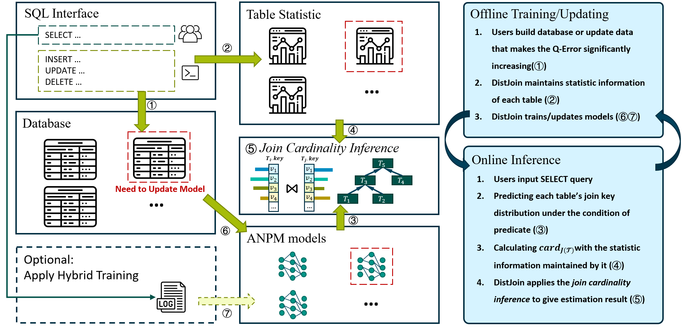
Figure 1: Overview of DistJoin. DistJoin maintains a lightweight autoregressive ANPM model and statistical information for each table, including each column’s NDV (Number of Distinct Values) and join key column distribution. Models are offline-trained (and updated) for online inference. Historical workloads can optionally enhance accuracy on small datasets through hybrid training.

1. Estimating Joint Distribution of the Join Key and Predicates: DistJoin first estimates each table’s join key distribution under predicate conditions $\mathcal{Q}(T_{i})$ (step ➂). This distribution, denoted by $\hat{P}_{T_{i}}(T_{i}.C_{key},\mathcal{Q}(T_{i}))$, identifies the selectivity per key participating in the join under condition of given predicates $\mathcal{Q}(T_{i})$.

2. Calculating Join Schema Cardinality. To mitigate variance accumulation, DistJoin calculates join schema cardinality $card_{J}(\mathcal{T})$ and multiplies it by the predicates-filtered join query’s selectivity (as in Equation 2), rather than simply applying the inner product on each table’s join key distribution like FactorJoin does (as in Equation 3). DistJoin efficiently computes $card_{J}(\mathcal{T})$ using maintained key column distributions through the process shown in Equation 28 (step ➃).

3. Selectivity-based Join Cardinality Inference. With join schema cardinality and joint distributions of key and predicates, DistJoin calculates selectivity bottom-up through the join tree (join order independent) and multiplies by join schema cardinality to obtain the final estimate.

DistJoin’s design differs fundamentally from existing methods:

Comparison with NeuroCard: While NeuroCard couples all tables and fanout values to estimate full outer join view probabilities, DistJoin preserves inter-table correlations through key distributions by maintaining lightweight autoregressive models and statistical information per table. This enables independent, on-demand model updates when individual tables’ data changes.

Comparison with FactorJoin: FactorJoin employs binning to handle large join key domains, sacrificing accuracy. In contrast, DistJoin’s efficient distribution estimation directly computes complete join key distributions, eliminating binning errors and supporting equi joins, non-equi joins, and outer joins with high accuracy. Additionally, DistJoin calculates join query selectivity using estimated distributions and multiplies by efficiently computed join schema cardinality $card_{J(\mathcal{T})}$, mitigating variance accumulation - a key improvement over FactorJoin’s direct calculation approach.

The remainder of this paper details DistJoin’s join key distribution estimation in section 5 and its selectivity-based join cardinality inference in section 6.

5 Individual Table’s Distribution Estimation

This section introduces our Adaptive Neural Predicate Modulation and its role in estimating each table’s key distribution $\hat{P}_{T_{i}}(T_{i}.C_{key},\mathcal{Q}(T_{i}))$.

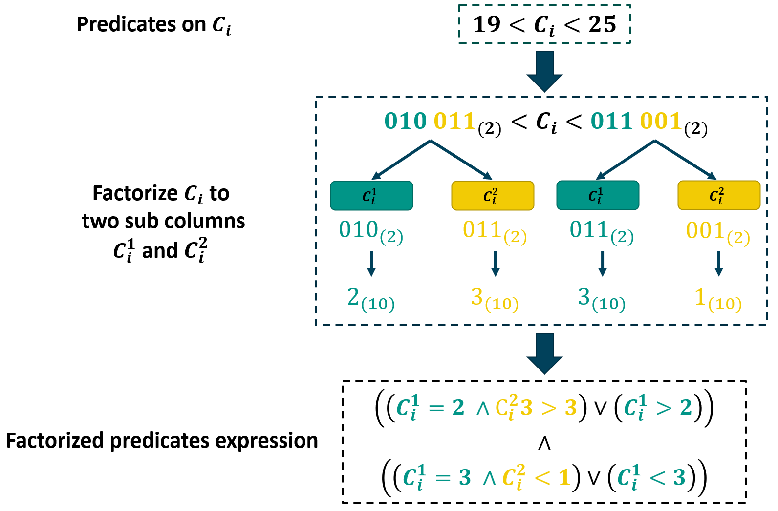
(a)

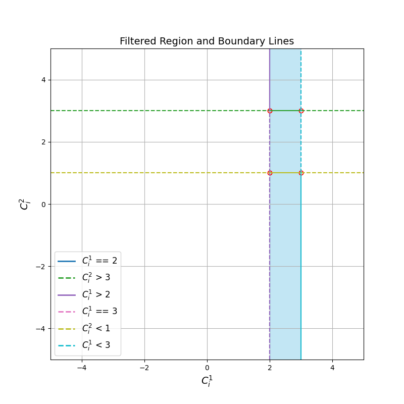
(b)

Figure 2: Example of factorized predicates’ filtered region and boundary. The filtered region on sub-columns forms a multi-dimensional cube with complex boundaries, where both predicate expression complexity and boundary complexity increase with sub-column count.

5.1 Predicates Lossless Factorization

Naru [50] introduced a significant advancement by formulating single-table cardinality estimation as an autoregressive process. However, its reliance on progressive sampling for range queries necessitates thousands of samples and multiple neural network forward passes per estimation. This approach becomes infeasible for join key columns where $|\mathcal{D}(T_{i}.C_{key})|$ can reach $10^{8}$, as estimating $\hat{P}_{T_{i}}(T_{i}.C_{key},\mathcal{Q}(T_{i}))$ would require storing and processing a multi-dimensional array exceeding $R^{2k\times 1e8}$ dimensions (with typical sampling size $k=2000$). BayesCard [48] similarly struggles with estimating probabilities for millions of distinct join key values within practical time constraints. These limitations force existing methods to adopt compromise techniques like binning and sampling, despite their drawbacks in accuracy, non-equi join support, and update flexibility.

DistJoin builds upon our previous single-table estimator Duet [52], detailed in subsection 3.3. While Duet eliminates sampling and predicts complete probability distributions in a single forward inference, its inference time and memory costs remain high for large domain sizes due to high-dimensional embedding layers and output distributions - a common challenge for join key columns.

NeuroCard’s lossless column factorization technique [49] addresses this by converting columns with large domains into binary representations and splitting them into sub-columns. This reduces domain size from $|\mathcal{D}(C)|$ to less than $m\times 2^{\lceil\frac{\lfloor log_{2}(|\mathcal{D}(C)|)\rfloor+1}{m}\rceil}$, where $m$ is the number of sub-columns. However, this technique is incompatible with Duet’s predicate-based input approach.

As shown in Figure 2, applying column factorization to predicate values significantly increases the complexity of the predicate expression. For instance, the predicate $19<C_{i}<25$ has a simple boundary when unfactorized but becomes a complex nested logical expression after factorization, as illustrated in 2(a). 2(b) demonstrates that while the filtered region remains a hypercube, its boundary becomes a complex piecewise hyperplane, with complexity growing with sub-column count.

For a predicate $C_{i}>v$, let $k_{i}$ denote the number of sub-columns from $C_{i}$’s factorization, and let $C_{i}^{j}$ and $v_{i}^{j}$ represent the $j$-th factorized column and predicate value respectively (with $j=0$ as the highest bit). The factorized predicate expression becomes:

$$(C_{i}^{0}>v_{i}^{0})\ \lor\ (C_{i}^{0}=v_{i}^{0}\land C_{i}^{1}>v_{i}^{1})\ \lor\ \dots\ \lor\ (C_{i}^{0}=v_{i}^{0}\land\dots\land C_{i}^{j}=v_{i}^{j}\land\dots\land C_{i}^{k_{i}}>v_{i}^{k_{i}})$$ (6)

To address this challenge, we embed both original and factorized predicate information into the input vector. As shown in Equation 6, predicate factorization follows a consistent pattern: $n_{i}$ conjunctive clauses connected by disjunctions, where only the final term’s predicate operator matches the original predicate, while preceding terms use equality operators. This pattern enables lossless value factorization without directly encoding complex logical expressions. For example, the predicate $C_{i}>v_{i}$ factorizes into $(C_{i}^{1}>v_{i}^{1},\dots,C_{i}^{k_{i}}>v_{i}^{k_{i}})$, where $v_{i}^{j}$ represents the factorized value corresponding to each sub-column.

For multiple predicates on the same original column, as illustrated in Figure 3, DistJoin first factorizes and embeds each column’s predicates independently. Following Duet’s approach, it then sums the predicate embedding vectors for each sub-column to form the input for our ANPM model, which we detail in the following subsection.

5.2 Adaptive Neural Predicate Modulation

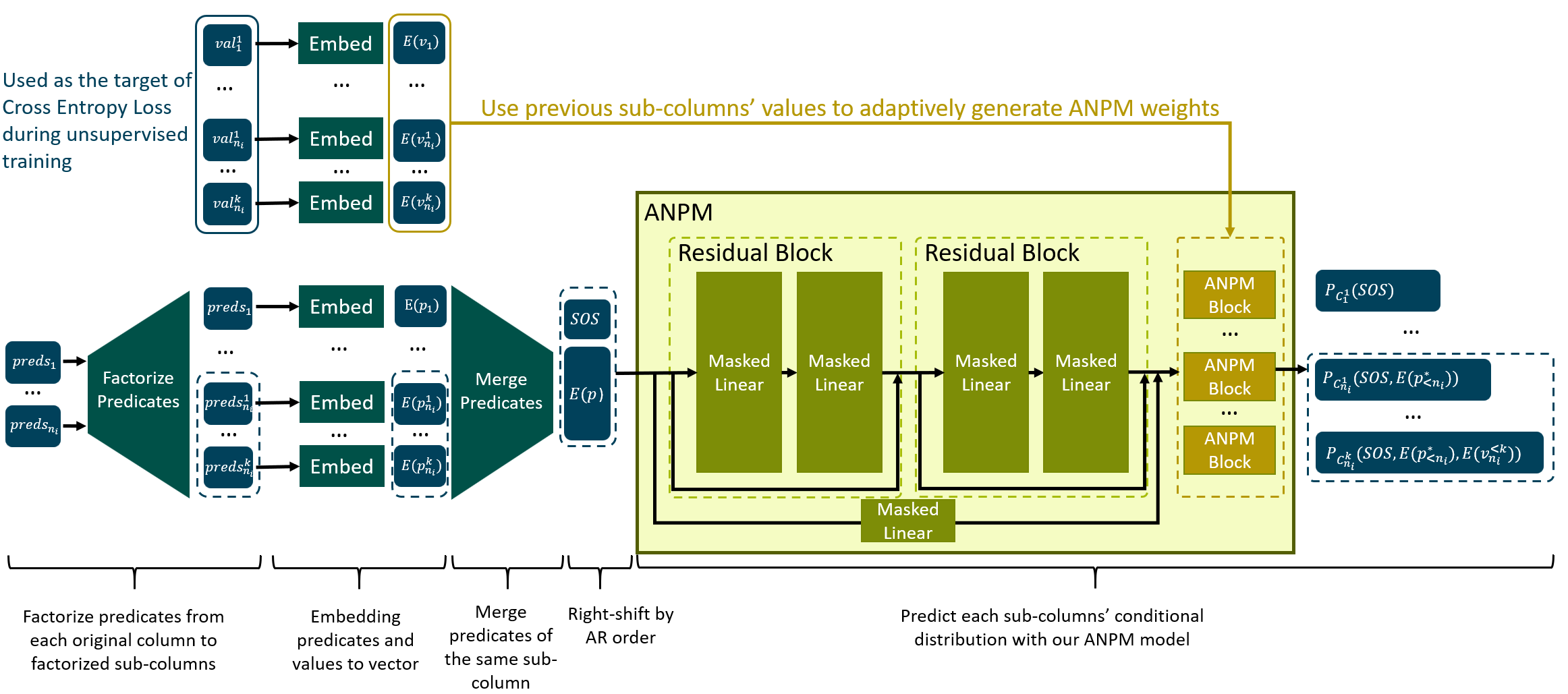
Figure 3: Architecture of Single Table’s Distribution Estimator. Predicates are first factorized using the method introduced in subsection 5.1. Each sub-column’s tuple values and factorized predicates are then embedded into vectors, with predicate vectors from the same column merged. Finally, an ANPM network predicts each sub-column’s conditional distribution under given factorized predicates and values. Note: We employ Naru’s wildcard-skipping technique [50, 49] for columns not constrained by predicates by replacing the original column predicates with learnable weights during training.

The predicate factorization method provides lossless predicate semantics for $C_{i}$ (or its sub-columns) based on preceding original columns $C_{<i}$. However, for $C_{i}^{j}$, this approach alone cannot handle factorized predicate constraints from preceding $j-1$ sub-columns.

From Equation 6 and 2(b), we observe that the $j$-th sub-column $C_{i}^{j}$’s probability distribution depends on factorized predicates from the first $j-1$ sub-columns of the same original column. Taking $C_{i}>v_{i}$ as an example, simply making the $j$-th sub-column’s distribution depend on these predicates would yield $\hat{P}(C_{i}^{j}|C_{i}^{1}>v_{i}^{1}\land\dots,\land C_{i}^{j-1}>v_{i}^{j-1})$, which is incorrect since conditions should follow Equation 6, leading to selectivity underestimation. The core issue lies in common autoregressive models (e.g., Transformer, MADE) only representing conjunctive relationships through autoregressive masks, unable to handle complex logical expressions involving disjunctions within one inference.

Another challenge is reconstructing original column distributions from sub-column distributions for selectivity estimation using Equation 4 and Equation 5. DistJoin reconstructs the original column’s distribution through Algorithm 1. Line 3 applies element-wise product between distribution $\mathbf{\hat{P}}(C_{i}^{<j}|preds_{<i})$ and estimated multi-dimensional distribution $\mathbf{\hat{P}}(C_{i}^{j}|C_{i}^{<j},preds_{<i})\in R^{\prod_{1}^{n}|\mathcal{D}(C_{i}^{j})|}$. Intuitively, since the sub-columns are arranged from high to low bits [49], the column dimension of the element-wise product result represents the distinct value combinations of lower-bit sub-columns, while the row dimension represents all possible permutations of distinct values from higher-bit sub-columns. By unfolding the result in row-major order, we obtain the probability distribution of all distinct values for the original column. This lossless reconstruction requires estimating $\hat{P}(C_{i}^{1},pred_{<i})\in R^{|\mathcal{D}(C_{i}^{1})|},\dots,\hat{P}(C_{i}^{n}|C_{i}^{<n},pred_{<i})\in R^{\prod_{1}^{n}{|\mathcal{D}(C_{i}^{j})|}}$, necessitating $n$ inference steps with up to $\prod_{1}^{n}{|\mathcal{D}(C_{i}^{j})|}$ inputs per inference for each original column. This approach proves infeasible due to excessive time and GPU memory requirements during training.

Input: Sub-columns’ predicate distributions:

$\mathbf{\hat{P}}(C_{i}^{1}|preds_{<i})\in R^{|\mathcal{D}(C_{i}^{1})|}$,

$\mathbf{\hat{P}}(C_{i}^{2}|C_{i}^{1},preds_{<i})\in R^{|\mathcal{D}(C_{i}^{1})|\times|\mathcal{D}(C_{i}^{2})|}$,

…,

$\mathbf{\hat{P}}(C_{i}^{n}|C_{i}^{<n},preds_{<i})\in R^{\prod_{1}^{n}|\mathcal{D}(C_{i}^{j})|}$,

where $preds_{<i}$ represents predicates on all columns or sub-columns preceding $C_{i}$ in the autoregressive order.

Output: Reconstructed original column’s distribution $\mathbf{\hat{P}}(C_{i}|preds_{<i})$

1 $\mathbf{Dist}\longleftarrow\mathbf{\hat{P}}(C_{i}^{1}|preds_{<i})$;

2 for $j\in[2,n]$ do

3    $\mathbf{Dist}\longleftarrow$ flatten($\mathbf{Dist}\text{.unsqueeze(1)}\odot\mathbf{\hat{P}}(C_{i}^{j}|C_{i}^{<j},preds_{<i})$);   // $\mathbf{Dist}=\mathbf{\hat{P}}(C_{i}^{\leq j}|preds_{<i})$ here

4   

5$\mathbf{Dist\_Slice}\longleftarrow\mathbf{Dist}[:|\mathcal{D}(C_{i})|]$;   // Drop non-existent combinations

6 $\mathbf{Dist}\longleftarrow\mathbf{Dist}\text{.sum()}/\mathbf{Dist\_Slice}\text{.sum()}$;   // Normalization

7 return $\mathbf{Dist}$;

Algorithm 1 Lossless Reconstruction for Original Column’s Distribution

To address these challenges, we designed the ANPM model, illustrated in Figure 3 and Figure 4. The ANPM comprises a ResMADE network [6, 33, 50], six ANPM HyperNetworks per factorized column, and a learned softmax temperature coefficient.

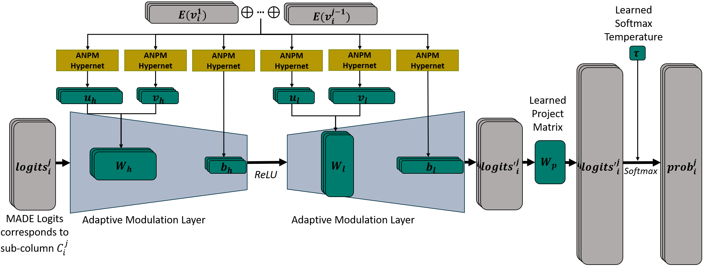
Figure 4: Architecture of the ANPM Block. DistJoin constructs an ANPM block for each factorized column, utilizing six lightweight MLPs (ANPM HyperNet) to predict low-rank decomposition results for adaptive modulation layer weight matrices and bias vectors. The two generated adaptive modulation layers form a bottleneck network, modulating $C_{i}^{j}$ values into MADE’s output logit corresponding to $C_{i}^{j}$, ultimately yielding the estimated probability distribution $P(C_{i}^{j}|E(p_{<i}^{*}),E(v_{i}^{<j}))$ through a projection matrix and learnable softmax temperature coefficient.

The ResMADE network’s autoregressive order and masks are carefully designed. From the perspective of original columns, the order is arbitrary, except the join key column must be last. From the perspective of factorized columns, sub-columns from the same original column are placed adjacently, ordered from higher to lower bits. We address a fitting capability limitation in previous works [50, 49] where the first distribution predicted by MADE (or ResMADE) [6, 33] was independent of inputs, relying solely on the last linear layer’s bias. Inspired by NLP techniques, we introduce an SOS (start of sequence) token at the beginning of the input sequence and right-shift the input sequence order to improve the accuracy of the first column distribution prediction. The SOS token remains at the autoregressive sequence’s start.

Autoregressive masks adhere to constraints where output corresponding to $C_{i}^{j}$ depends on any $E(p_{<i}^{*})$ predicate inputs but not $E(p_{\geq i}^{*})$, maintaining autoregressive dependency constraints from the original columns’ perspective. Thus, ResMADE’s output $logits_{i}^{j}$ is predicted based on preceding $i-1$ original columns’ predicates.

To balance complex non-linear inter-column correlations with model training and inference speed, we implement a learnable mixed activation layer. This layer applies different activation functions to ResMADE’s final layer output and outputs their weighted sum, enhancing model representational capacity. To further adapt the high skewness column, we employ a learned temperature coefficient for each sub-column’s softmax activation function.

For factorized predicates, we modify Duet’s approach: instead of predicate-based input for same-original-column sub-columns, we embed true values of first $j-1$ sub-columns and input them into the ANPM Block during training, similar to Naru. As shown in Figure 4, the ANPM Block employs six lightweight HyperNetworks (2-layer MLPs with 64-unit width) to predict low-rank decomposition results for weight matrices and bias vectors. Matrix multiplication reconstructs weights for two linear adaptive modulation layers, embedding first $j-1$ sub-columns’ true values into their weights and biases. By sizing these layers appropriately, they form a bottleneck MLP, further optimizing calculations. This MLP modulates information from the first $j-1$ sub-columns into $logits_{i}^{j}$ during transformation.

ANPM’s calculation for $C_{i}^{j}$ follows these formulas, with distinct embedding approaches for training and inference. As shown in Equation 7, ANPM concatenates factorized true value embedding vectors during training. During inference, ANPM generates combinations of the first $j-1$ sub-columns’ distinct values along the batch dimension, avoiding dimensional explosion as shown in Equation 8.

$$\overset{(B,F)}{x} =\overset{(B,E)}{E(v_{i}^{1})}\oplus\overset{(B,E)}{E(v_{i}^{2})}\oplus\cdots\oplus\overset{(B,E)}{E(v_{i}^{j-1})}$$ (7)

$$\overset{(B,F)}{x} =(\dots(\overset{(|\mathcal{D}(C_{i}^{1})|,1,E)}{E(v_{i}^{1}).\text{unsqueeze(1)}}\oplus\overset{(1,|\mathcal{D}(C_{i}^{1})|,E)}{E(v_{i}^{2}).unsqueeze(0)}).unsqueeze(1)\oplus\cdots)\oplus\overset{(|\mathcal{D}(1,C_{i}^{1})|,E)}{E(v_{i}^{j-1}).unsqueeze(0)}$$ (8)

, where $$F=(j-1)\times E B=\text{batch\_size} B=\prod_{1}^{j-1}|\mathcal{D}(C_{i}^{j})|$$ and during training and during inference. Then, the ANPM projects the logits by the following formulas:

$$\overset{(B,F,1)}{u_{h}} =\text{unsqueeze}(\text{HyperNet}_{h}^{u}(x),2),\quad\overset{(B,1,E)}{v_{h}}=\text{unsqueeze}(\text{HyperNet}_{h}^{v}(x),1),\quad\overset{(B,E)}{b_{h}}=\text{HyperNet}_{h}^{b}(x)$$ (9)

$$\overset{(B,E,1)}{u_{l}} =\text{unsqueeze}(\text{HyperNet}_{l}^{u}(x),2),\quad\overset{(B,1,F)}{v_{l}}=\text{unsqueeze}(\text{HyperNet}_{l}^{v}(x),1),\quad\overset{(B,F)}{b_{l}}=\text{HyperNet}_{l}^{b}(x)$$ (10)

$$\overset{(B,F,E)}{W_{h}} =u_{h}\times v_{h},\quad\overset{(B,E,F)}{W_{l}}=u_{l}\times v_{l}$$ (11)

$$\overset{(B,F)}{logits_{i}^{\prime j}} =ReLU(\overset{(B,F)}{logits_{i}^{j}}\times W_{h}+b_{h})\times W_{l}+b_{l}$$ (12)

Finally, ANPM calculates the distribution as $\hat{P}(C_{i}^{j}|C_{i}^{1}=val_{i}^{1},\dots,C_{i}^{j-1}=val_{i}^{j-1},preds_{<i})\in R^{(\text{batch\_size},|\mathcal{D}(C_{i}^{j})|)}$ during training and $\hat{P}(C_{i}^{j}|C_{i}^{1},\dots,C_{i}^{j-1},preds_{<i})\in R^{\prod_{1}^{j}|\mathcal{D}(C_{i}^{j})|}$ during inference.

The key advantage of ANPM lies in its ability to decouple predicate processing from factorized value combination handling. By employing dedicated ANPM blocks for each sub-column, the ResMADE component focuses exclusively on processing predicate information. The ANPM blocks efficiently handle all possible combinations of factorized values from $Col_{i}^{<j-1}$. This architecture enables ResMADE, the most computationally intensive component, to perform parallel inference across all sub-columns during the column distribution reconstruction phase, where the model must predict $\hat{P}(C_{i}^{j}|C_{i}^{1},\dots,C_{i}^{j-1},preds_{<i})$.

Without ANPM, ResMADE would be unable to simultaneously represent all sub-column values of $Col_{i}$ and the factorized predicates in a single input. This limitation would necessitate processing each original column’s sub-columns sequentially: feeding ResMADE with all factorized predicates from $Col_{<i}$ while iterating through all possible values of $Col_{i}^{<j-1}$. This approach, similar to NeuroCard’s method, would require multiple large-scale inference passes, significantly compromising estimation efficiency.

Scalability Analysis. Considering NeuroCard’s column factorization with 14-bit width as an example, for two factorized columns, the maximum batch dimension size during inference is $2^{14}=16384$, matching our experimental training batch size. This scale is efficiently supported since inference excludes backward propagation compared to training. Therefore, this method effectively supports original columns with up to $2^{28}$ distinct values, approaching the uint32 type limit commonly used for primary key IDs in DBMSs. Thus, our method accommodates most database scenarios. For extreme cases exceeding this limit, accuracy can be traded by bucketing columns with no more than $2^{4}$ elements per bucket. Compared to FactorJoin’s bucketing strategy, this approach yields shallower buckets and reduced accuracy loss.

Training. DistJoin employs Duet’s method for training sample generation. Specifically, it randomly samples original and factorized tuples from the table, using Duet’s predicate generation algorithm to create predicate inputs constraining these tuples. Factorized tuples serve dual purposes: as learning targets for cross-entropy loss (equivalent to NLL loss) and as inputs to the ANPM Block. Since the ANPM model trains through unsupervised learning, it’s not a label leakage. This training approach on factorized tables avoids calculations involving the original column’s large domain size.

Inference. During inference, ANPM Blocks utilize embedding weights containing all distinct values’ embedding vectors for each factorized column as inputs. The distinct values’ dimension serves as the batch dimension. Although this approach may appear resource-intensive, ANPM Blocks’ placement after ResMADE ensures ResMADE processes only a single sample during inference. Furthermore, ANPM Blocks employ lightweight MLP networks with low-rank decomposition, maintaining high efficiency even with thousands of sub-column distinct values. This method also prevents combinatorial explosion across different original columns. Experimental results confirm ANPM’s efficiency.

Finally, we reconstruct each original column’s distribution under proceeding predicates using algorithm 1. DistJoin then estimates individual table selectivity $\hat{p}(\mathcal{Q}(T))$ using Equation 4 and Equation 5, calculating $\hat{P}(C_{key},Q(T))=\hat{P}(C_{key}|Q(T))*\hat{p}(\mathcal{Q}(T))$.

6 Join Cardinality Inference Based On Single Tables’ Distribution

This section first analyzes the variance accumulation issue in FactorJoin’s join cardinality inference method Equation 3, then introduces DistJoin’s selectivity-based join cardinality inference approach.

6.1 Previous Method’s Variance Accumulation Problem

As discussed in subsection 3.2, FactorJoin pioneered join cardinality calculation using estimated join key distributions. While innovative and capable of providing unbiased results given unbiased probability estimates, the formula in Equation 3 suffers from severe variance accumulation, where variance scales with the square of the Cartesian product cardinality of joined tables (denoted by $\text{card}_{\mathcal{T}}=\prod_{i=1}^{n}|T_{i}|$).

Theorem 1.

Given the join cardinality inference method defined in Equation 3, let card be the true cardinality and $p_{i}(v,\mathcal{Q})$ be the true probability, the expectation and variance of the estimation result satisfy:

$$\mathbb{E}[\hat{\text{card}}] =\sum_{v}\prod_{i=1}^{N}|T_{i}|p_{i}(v,\mathcal{Q})=\text{card}$$ (13)

$$\text{Var}(\hat{\text{card}}) \propto\prod_{i=1}^{N}|T_{i}|^{2}$$ (14)

Before proving Theorem 1, we establish that neural network probability estimation errors follow an arbitrary distribution $\mathcal{G}$. This represents a relaxed constraint compared to typical assumptions of normal distribution in related works [8, 18, 12]. Since our analysis focuses on join cardinality inference accuracy, we also assume unbiased probability estimates for individual tables, implying $\mathbb{E}[\mathcal{G}]=0$.

Assumption 1.

For convenience and clarity, let the bin depth be 1, thus $bin(v)=v$ and $p_{i}(\cdot)$ is the true probability. We assume the error of predicted probability follows:

$$\hat{p}_{T_{i}}(T_{i}.C_{key} =v,\mathcal{Q}(T_{i}))=p_{i}(v,\mathcal{Q})+\epsilon_{i}(v,\mathcal{Q}),\quad\epsilon_{i}(v,\mathcal{Q})\sim\mathcal{G}(0,\sigma_{i}^{2}(v,\mathcal{Q}))$$ (15)

$$\hat{p}_{T_{i}}(T_{i}.C_{key} =v)=p_{i}(v)+\epsilon_{i}(v),\quad\epsilon_{i}(v)\sim\mathcal{G}(0,\sigma_{i}^{2}(v))$$ (16)

, where $\mathcal{G}(\mu,\sigma^{2})$ represents an arbitrary distribution with expectation $\mu$ and variance $\sigma^{2}$.

Proof of Theorem 1. Since each table has an independent estimator, the estimated probability of each table is independent. Thus ,  Equation 13 can be proved by:

$$\mathbb{E}[\hat{\text{card}}] =\mathbb{E}\left[\sum_{v}\prod_{i=1}^{N}\hat{p}_{T_{i}}(T_{i}.C_{key}=v,\mathcal{Q}(T_{i}))|T_{i}|\right]$$ (17)

$$=\sum_{v}\prod_{i=1}^{N}|T_{i}|\mathbb{E}\left[\hat{p}_{T_{i}}(T_{i}.C_{key}=v,\mathcal{Q}(T_{i}))\right]$$ by linearity of expectation (18)

$$=\sum_{v}\prod_{i=1}^{N}|T_{i}|p_{i}(v)$$ (19)

Next, we prove the variance is proportional to $\prod_{i=1}^{n}|T_{i}|^{2}$. Based on the designs that both FactorJoin and DistJoin employ independent models to estimate different tables, there are the following facts:

1. Since the prediction errors among different key values of the same table are related: $\text{Cov}(\epsilon(v,\mathcal{Q}),\epsilon(v^{\prime},\mathcal{Q}))=C_{i}^{Q}(v,v^{\prime})$

2. Since prediction errors among different tables are independent: $\text{Cov}(\epsilon_{i}(v,\mathcal{Q}),\epsilon_{j}(v^{\prime},\mathcal{Q}))=0,\quad(i\neq j)$

Expanding the  Equation 3 by:

$$\hat{\text{card}} =\prod_{i=1}^{n}|T_{i}|\sum_{v}\prod_{i=1}^{n}\hat{p}_{i}(v,\mathcal{Q})$$ (20)

$$=\prod_{i=1}^{n}|T_{i}|\sum_{v}\prod_{i=1}^{n}\left(p_{i}(v,\mathcal{Q})+\epsilon_{i}(v,\mathcal{Q})\right)$$ (21)

$$=\prod_{i=1}^{n}|T_{i}|\cdot X,\quad\quad X=\sum_{v}\prod_{i=1}^{n}\left(p_{i}(v,\mathcal{Q})+\epsilon_{i}(v,\mathcal{Q})\right)$$ (22)

The variance of estimated cardinality is:

$$\text{Var}(\hat{\text{card}}) =\left(\prod_{i=1}^{n}|T_{i}|\right)^{2}\text{Var}\left(X\right)$$ (23)

$$\propto\left(\prod_{i=1}^{n}|T_{i}|\right)^{2}\qquad\text{By $X$ is independent of $|T_{i}|$ since $p_{i}$ is normalized probability}$$ (24)

∎

6.2 DistJoin’s Equi Join Estimation Approach

As demonstrated, $\prod_{i=1}^{n}|T_{i}|^{2}$ and $\text{Var}(\hat{card})$ grow rapidly with increasing join tables and table cardinalities. To address this, we propose a novel selectivity-based join cardinality inference approach.

This method recursively computes, from the bottom up along the join plan tree, the proportion of each join key value under predicate filtering in the unfiltered join result $J(\mathcal{T})$. Summing these proportions yields the overall query selectivity. Combined with the maintained key column distribution information used to calculate the true cardinality $\text{card}_{J(\mathcal{T})}$ via Equation 28, multiplying selectivity by this cardinality produces the final estimate. The process is formalized as:

$$\hat{p}_{\{T_{l},T_{r}\}}(key=v,\mathcal{Q}) =\frac{\hat{p}_{T_{l}}(T_{l}.C_{key}=v,\mathcal{Q}(T_{l}))*\hat{p}_{T_{r}}(T_{r}.C_{key}=v,\mathcal{Q}(T_{r}))}{\sum_{v\in\mathcal{D}(T_{l}.C_{key})\cup\mathcal{D}(T_{r}.C_{key})}\hat{p}_{T_{l}}(T_{l}.C_{key}=v)*\hat{p}_{T_{r}}(T_{r}.C_{key}=v)}$$ (25)

$$\hat{p}_{\mathcal{T}}(key=v,\mathcal{Q}) =\frac{\hat{p}_{\mathcal{T}_{left}}(key=v,\mathcal{Q})*\hat{p}_{\mathcal{T}_{right}}(key=v,\mathcal{Q})}{\sum_{v\in\mathcal{D}(\mathcal{T})}{\hat{p}_{\mathcal{T}_{left}}(key=v)*\hat{p}_{\mathcal{T}_{right}}(key=v)}}$$ (26)

$$\mathcal{T}_{\text{left}} =\{T_{1},T_{2},\dots,T_{\lfloor N/2\rfloor}\},\mathcal{T}_{\text{right}}=\{T_{\lfloor N/2\rfloor+1},\dots,T_{N}\}$$ (27)

$$\text{card}_{J(\mathcal{T})} =\sum_{v\in\cup_{i=1}^{N}\mathcal{D}(T_{i}.C_{key})}\prod_{i\in[1,N]}p_{T_{i}}(T_{i}.C_{key}=v)|T_{i}|$$ (28)

$$\hat{\text{card}} =\text{card}_{J(\mathcal{T})}*\sum_{v\in\mathcal{D}(\mathcal{T})}\hat{p}_{\mathcal{T}}(\mathcal{Q})$$ (29)

Here, $\mathcal{T}$ denotes the join table set, $card_{J(\mathcal{T})}$ represents the join schema cardinality on $\mathcal{T}$, and $p_{T_{i}}(T_{i}.C_{key})$ indicates the true distribution probability of the join key column. Equation 25 presents the base case for two-table joins, while Equation 26 and Equation 27 define the recursive formulas. Equation 28 calculates the join schema cardinality, which DistJoin caches for reuse. Finally, Equation 29 computes the final estimate by multiplying the summed selectivity by $\text{card}_{J(\mathcal{T})}$.

Notably, DistJoin avoids conditional independence assumptions despite Equation 25 and Equation 26’s apparent similarity to such assumptions. This is demonstrated by:

$$\hat{p}_{\{T_{l},T_{r}\}}(key=v,\mathcal{Q}) =\frac{\left[\hat{p}_{T_{l}}(T_{l}.C_{key}=v,\mathcal{Q}(T_{l}))\cdot|T_{l}|\right]*\left[\hat{p}_{T_{r}}(T_{r}.C_{key}=v,\mathcal{Q}(T_{r}))\cdot|T_{r}|\right]}{\sum_{v\in\mathcal{D}(T_{l}.C_{key})\cup\mathcal{D}(T_{r}.C_{key})}\left[\hat{p}_{T_{l}}(T_{l}.C_{key}=v)\cdot|T_{l}|\right]*\left[\hat{p}_{T_{r}}(T_{r}.C_{key}=v)\cdot|T_{r}|\right]}$$ (30)

$$=\frac{\hat{p}_{T_{l}}(T_{l}.C_{key}=v,\mathcal{Q}(T_{l}))*\hat{p}_{T_{r}}(T_{r}.C_{key}=v,\mathcal{Q}(T_{r}))}{\sum_{v\in\mathcal{D}(T_{l}.C_{key})\cup\mathcal{D}(T_{r}.C_{key})}\hat{p}_{T_{l}}(T_{l}.C_{key}=v)*\hat{p}_{T_{r}}(T_{r}.C_{key}=v)}$$ (31)

The numerator of Equation 30 computes the cardinality under predicates $\mathcal{Q}(T_{l})$ and $\mathcal{Q}(T_{r})$ for join key $v$, while the denominator calculates the unconditional join cardinality. The $|T_{l}||T_{r}|$ terms cancel, eliminating independence assumptions.

Under the assumptions in Assumption 1 and  Assumption 2, this approach provides unbiased estimates with variance proportional to $\text{card}_{J(\mathcal{T})}^{2}$, as proven in subsection 6.3.

Inference Efficiency. Leveraging ANPM’s high estimation efficiency, this process avoids the computational expense suggested by the formulas. ANPM estimates complete join key column distributions, enabling full utilization of GPU parallel computation or CPU AVX instructions. For two-table joins, DistJoin employs vectorized calculation:

$$\hat{\mathbf{P}}_{\mathcal{T}}(KEY,\mathcal{Q}) =\frac{\hat{\mathbf{P}}_{\mathcal{T}_{left}}(KEY,\mathcal{Q})\odot\hat{\mathbf{P}}_{\mathcal{T}_{right}}(KEY,\mathcal{Q})}{\hat{\mathbf{P}}_{\mathcal{T}_{left}}(KEY)\cdot\hat{\mathbf{P}}_{\mathcal{T}_{right}}(KEY)}$$ (32)

Here, denominator vectors follow consistent distinct value encoding and are recursively calculated using the same formula with $\mathcal{Q}=\emptyset$. The algorithm appears in algorithm 2. DistJoin also supports outer joins by assigning probability 1 to non-existent join key values in corresponding tables before performing equi-joins.

6.3 Expectation and Variance Analysis with Comparative Insights

This subsection presents an expectation and variance analysis for equi joins, comparing DistJoin’s performance with FactorJoin’s approach.

Theorem 2.

Let $card$ denote the true cardinality and $p_{T}(\cdot)$ represent the true probability. The expectation and variance of DistJoin’s equi join cardinality inference process satisfy:

$$\mathbb{E}[\hat{\text{card}}] \approx\text{card}_{J(\mathcal{T})}\frac{\sum_{v}p_{T_{l}}(v,\mathcal{Q})p_{T_{r}}(v,\mathcal{Q})}{\sum_{v}p_{T_{l}}(v)p_{T_{r}}(v)}=\text{card}$$ (33)

$$\text{Var}(\hat{\text{card}}) \propto\text{card}_{J(\mathcal{T})}^{2}$$ (34)

Assumption 2.

For analytical convenience, we assume zero covariance between distribution estimates under different inputs:

$$\text{Cov}(f(X_{1}),f(X_{2}))=0,\ \text{where}\ f(\cdot)\ \text{is an estimator}$$ (35)

Proof of Theorem 2. We first analyze the expectation and variance of the two-table joins situation:

$$\hat{\text{card}} =\text{card}_{J(\mathcal{T})}\frac{\sum_{v}\hat{p}_{T_{l}}(v,\mathcal{Q})\hat{p}_{T_{r}}(v,\mathcal{Q})}{\sum_{v}\hat{p}_{T_{l}}(v)\hat{p}_{T_{r}}(v)}$$ (36)

By the  Assumption 1:

$$\mathbb{E}[\hat{p}_{T_{l}}(v,\mathcal{Q})] =p_{T_{l}}(v,\mathcal{Q}),\quad\mathbb{E}[\hat{p}_{T_{r}}(v,\mathcal{Q})]=p_{T_{r}}(v,\mathcal{Q}),\quad\mathbb{E}[\hat{p}_{T_{l}}(v)]=p_{T_{l}}(v),\quad\mathbb{E}[\hat{p}_{T_{r}}(v)]=p_{T_{r}}(v)$$ (37)

Let:

$$\hat{S_{\mathcal{Q}}} =\sum_{v}\hat{p}_{T_{l}}(v,\mathcal{Q})\hat{p}_{T_{r}}(v,\mathcal{Q}),\quad\hat{S}=\sum_{v}\hat{p}_{T_{l}}(v)\hat{p}_{T_{r}}(v)$$ (38)

$$S_{\mathcal{Q}} =\sum_{v}p_{T_{l}}(v,\mathcal{Q})p_{T_{r}}(v,\mathcal{Q}),\quad S=\sum_{v}p_{T_{l}}(v)p_{T_{r}}(v)$$ (39)

$$\Delta S_{\mathcal{Q}} =\hat{S_{\mathcal{Q}}}-S_{\mathcal{Q}},\quad\Delta S=\hat{S}-S$$ (40)

By using independent trained models for different tables and  Assumption 1:

$$\mathbb{E}[\hat{S_{\mathcal{Q}}}] =\sum_{v}p_{T_{l}}(v,\mathcal{Q})p_{T_{r}}(v,\mathcal{Q}),\quad\mathbb{E}[\hat{S}]=\sum_{v}p_{T_{l}}(v)p_{T_{r}}(v)$$ (41)

Taylor expansion of $$\frac{\hat{S_{\mathcal{Q}}}}{\hat{S}} \mathbb{E}[\hat{S}]$$ at :

$$\frac{\hat{S_{\mathcal{Q}}}}{\hat{S}} \approx\frac{\hat{S_{\mathcal{Q}}}}{\mathbb{E}[\hat{S}]}-\frac{\hat{S_{\mathcal{Q}}}(\hat{S}-\mathbb{E}[\hat{S}])}{\mathbb{E}[\hat{S}]^{2}}+\dots$$ (42)

$$\mathbb{E}\left[\frac{\hat{S_{\mathcal{Q}}}}{\hat{S}}\right] \approx\frac{\mathbb{E}[\hat{S_{\mathcal{Q}}}]}{\mathbb{E}[\hat{S}]}-\frac{\text{Cov}(\hat{S_{\mathcal{Q}}},\hat{S})}{\mathbb{E}[\hat{S}]^{2}}+\dots$$ (43)

By  Assumption 2, independent estimation for different tables and ignore the higher-order terms

$$\approx\frac{\mathbb{E}[\hat{S_{\mathcal{Q}}}]}{\mathbb{E}[\hat{S}]}$$ (44)

$$=\frac{\sum_{v}p_{T_{l}}(v,\mathcal{Q})p_{T_{r}}(v,\mathcal{Q})}{\sum_{v}p_{T_{l}}(v)p_{T_{r}}(v)}$$ (45)

$$\mathbb{E}[\hat{\text{card}}] =\text{card}_{J(\mathcal{T})}\mathbb{E}[\frac{\hat{S_{\mathcal{Q}}}}{\hat{S}}]\approx\text{card}_{J(\mathcal{T})}\frac{\sum_{v}p_{T_{l}}(v,\mathcal{Q})p_{T_{r}}(v,\mathcal{Q})}{\sum_{v}p_{T_{l}}(v)p_{T_{r}}(v)}=\text{card}$$ (46)

By $\text{card}_{J(\mathcal{T})}$ is a fixed value that is calculated based on true distribution, so it’s independent of either $\hat{S_{\mathcal{Q}}}$ or $S$:

$$\text{Var}(\hat{\text{card}}) =\text{Var}\left(\text{card}_{J(\mathcal{T})}\frac{\hat{S_{\mathcal{Q}}}}{\hat{S}}\right)=\text{card}_{J(\mathcal{T})}^{2}\text{Var}\left(\frac{\hat{S_{\mathcal{Q}}}}{\hat{S}}\right)$$ (47)

By Taylor expansion and ignoring higher-order terms:

$$\frac{\hat{S_{\mathcal{Q}}}}{\hat{S}} \approx\frac{S_{\mathcal{Q}}}{S}+\frac{\Delta S_{\mathcal{Q}}}{S}-\frac{S_{\mathcal{Q}}}{S^{2}}\Delta S$$ (48)

$$\text{Var}(\hat{\text{card}}) =\text{card}_{J(\mathcal{T})}^{2}\text{Var}\left(\frac{\hat{S_{\mathcal{Q}}}}{\hat{S}}\right)$$ (49)

$$\approx\text{card}_{J(\mathcal{T})}^{2}\left[\frac{\text{Var}(\Delta S_{\mathcal{Q}})}{S^{2}}+\frac{S_{\mathcal{Q}}^{2}}{S^{4}}\text{Var}(\Delta S)-2\frac{S_{\mathcal{Q}}}{S^{3}}\text{Cov}(\Delta S_{\mathcal{Q}},\Delta S)\right]$$ (50)

$$\propto\text{card}_{J(\mathcal{T})}^{2}$$ (51)

We can use induction to extend the conclusions above to n-table joins. For $k+1$ table joins situation: $T_{1}\Join\dots\Join T_{k+1}$, we regard it as $\mathcal{T}^{(k)}\Join T_{k+1}$, the cardinality can be calculated by:

$$\hat{\text{card}}^{(k+1)} =\text{card}_{J(\mathcal{T}^{(k+1)})}\frac{\sum_{v}\hat{p}_{\mathcal{T}^{(k)}}\left(v,\mathcal{Q}\left(\mathcal{T}^{(k)}\right)\right)\cdot\hat{p}_{T_{k+1}}\left(v,\mathcal{Q}\left(T_{k+1}\right)\right)}{\sum_{v}\hat{p}_{\mathcal{T}^{(k)}}(v)\hat{p}_{T_{k+1}}(v)}$$ (52)

$$\text{card}_{J(\mathcal{T}^{(k+1)})} =\sum_{v}\left[\text{card}_{J(\mathcal{T}^{(k)})}\cdot p_{\mathcal{T}^{(k)}}(v)\right]\cdot\left[|T_{k+1}|\cdot p_{T_{k+1}}(v)\right]$$ (53)

Since $\text{card}_{J(\mathcal{T}^{(k+1)})}$ is a fixed true value, we only need to prove that $\hat{p}_{\mathcal{T}^{(k)}}$ follows  Assumption 1. We proceed by mathematical induction:

Base Case ($k=1$): Based on  Assumption 1:

$$\hat{p}_{\mathcal{T}^{(1)}}(v,\mathcal{Q}) =p_{\mathcal{T}^{(1)}}(v,\mathcal{Q})+\epsilon_{\mathcal{T}^{(1)}}(v,\mathcal{Q}),\qquad\epsilon_{\mathcal{T}^{(1)}}(v,\mathcal{Q})\sim\mathcal{G}^{(1)}(0,\sigma_{1}^{2}(v,\mathcal{Q}))$$ (54)

$$\hat{p}_{\mathcal{T}^{(1)}}(v) =p_{\mathcal{T}^{(1)}}(v)+\epsilon_{\mathcal{T}^{(1)}}(v),\qquad\epsilon_{\mathcal{T}^{(1)}}(v)\sim\mathcal{G}^{(1)}(0,\sigma_{1}^{2}(v))$$ (55)

Inductive Hypothesis: Assuming the $k-1$-th join holds:

$$\hat{p}_{\mathcal{T}^{(k-1)}}(v,\mathcal{Q}) =p_{\mathcal{T}^{(k-1)}}(v,\mathcal{Q})+\epsilon_{\mathcal{T}^{(k-1)}}(v,\mathcal{Q}),\qquad\epsilon_{\mathcal{T}^{(k-1)}}(v,\mathcal{Q})\sim\mathcal{G}^{(k-1)}(0,\sigma_{k-1}^{2}(v,\mathcal{Q}))$$ (56)

$$\hat{p}_{\mathcal{T}^{(k-1)}}(v) =p_{\mathcal{T}^{(k-1)}}(v)+\epsilon_{\mathcal{T}^{(k-1)}}(v),\qquad\epsilon_{\mathcal{T}^{(k-1)}}(v)\sim\mathcal{G}^{(k-1)}(0,\sigma_{k-1}^{2}(v))$$ (57)

Inductive Step: We need to prove that for the $k$-th join, it holds:

$$\hat{p}_{\mathcal{T}^{(k)}}(v,\mathcal{Q}) =p_{\mathcal{T}^{(k)}}(v,\mathcal{Q})+\epsilon_{\mathcal{T}^{(k)}}(v,\mathcal{Q}),\qquad\epsilon_{\mathcal{T}^{(k)}}(v,\mathcal{Q})\sim\mathcal{G}^{(k)}(0,\sigma_{k}^{2}(v,\mathcal{Q}))$$ (58)

$$\hat{p}_{\mathcal{T}^{(k)}}(v) =p_{\mathcal{T}^{(k)}}(v)+\epsilon_{\mathcal{T}^{(k)}}(v),\qquad\epsilon_{\mathcal{T}^{(k)}}(v)\sim\mathcal{G}^{(k)}(0,\sigma_{k}^{2}(v))$$ (59)

Since in  Assumption 1, $\mathcal{G}^{(k)}$ is an arbitrary distribution and $\sigma_{k}^{2}$ is an arbitrary variance, we only need to prove that the expectation of the error $\epsilon_{\mathcal{T}^{(k)}}$ is zero.
By  Equation 26, we have:

$$\hat{p}_{\mathcal{T}^{(k)}}(v,\mathcal{Q}) =\frac{\hat{p}_{\mathcal{T}^{(k-1)}}\left(v,\mathcal{Q}\left(\mathcal{T}^{(k-1)}\right)\right)\cdot\hat{p}_{T_{k}}\left(v,\mathcal{Q}\left(T_{k}\right)\right)}{\sum_{v}\hat{p}_{\mathcal{T}^{(k-1)}}(v)\hat{p}_{T_{k}}(v)}$$ (60)

Let:

$$\hat{S}_{Q}^{(k)} =\hat{p}_{\mathcal{T}^{(k-1)}}\left(v,\mathcal{Q}\left(\mathcal{T}^{(k-1)}\right)\right)\cdot\hat{p}_{T_{k}}\left(v,\mathcal{Q}\left(T_{k}\right)\right),\quad\hat{S}^{(k)}=\sum_{v}\hat{p}_{\mathcal{T}^{(k-1)}}(v)\hat{p}_{T_{k}}(v)$$ (61)

$$S_{\mathcal{Q}}^{(k)} =p_{\mathcal{T}^{(k-1)}}\left(v,\mathcal{Q}\left(\mathcal{T}^{(k-1)}\right)\right)\cdot p_{T_{k}}\left(v,\mathcal{Q}\left(T_{k}\right)\right),\quad S^{(k)}=\sum_{v}p_{\mathcal{T}^{(k-1)}}(v)p_{T_{k}}(v)$$ (62)

$$\Delta S_{\mathcal{Q}}^{(k)} =\hat{S}_{Q}^{(k)}-S_{\mathcal{Q}}^{(k)},\qquad\Delta S^{(k)}=\hat{S}^{(k)}-S^{(k)}$$ (63)

Similar to the formula Equation 43, by Taylor expansion, we can be obtained:

$$\mathbb{E}\left[\hat{p}_{\mathcal{T}^{(k)}}(v,\mathcal{Q})\right] \approx\frac{\mathbb{E}\left[\hat{S_{\mathcal{Q}}}^{(k)}\right]}{\mathbb{E}\left[\hat{S}^{(k)}\right]}-\frac{\text{Cov}\left(\hat{S_{\mathcal{Q}}}^{(k)},\hat{S}^{(k)}\right)}{\mathbb{E}\left[\hat{S}^{(k)}\right]^{2}}+\dots$$ (64)

By  Assumption 2 and independent estimation between different tables:

$$\approx\frac{\mathbb{E}\left[\hat{S_{\mathcal{Q}}}^{(k)}\right]}{\mathbb{E}\left[\hat{S}^{(k)}\right]}$$ (65)

By using independent trained models for different tables and the inductive hypothesis:

$$=\frac{S_{\mathcal{Q}}^{(k)}}{S^{(k)}}$$ (66)

Because :

$$\mathbb{E}\left[\hat{p}_{\mathcal{T}^{(k)}}(v,\mathcal{Q})\right] =\mathbb{E}\left[p_{\mathcal{T}^{(k)}}(v,\mathcal{Q})+\epsilon_{\mathcal{T}^{(k)}}(v,\mathcal{Q})\right]$$ (67)

$$=p_{\mathcal{T}^{(k)}}(v,\mathcal{Q})+\mathbb{E}\left[\epsilon_{\mathcal{T}^{(k)}}(v,\mathcal{Q})\right]$$ (68)

$$=\frac{S_{\mathcal{Q}}^{(k)}}{S^{(k)}}+\mathbb{E}\left[\epsilon_{\mathcal{T}^{(k)}}(v,\mathcal{Q})\right]$$ (69)

We can obtain that:

$$\mathbb{E}\left[\epsilon_{\mathcal{T}^{(k)}}(v,\mathcal{Q})\right] =0$$ (70)

End of Induction Proof. Thus, because the base case holds and the inductive step holds, we proved that for $N$-table joins, the $\epsilon_{\mathcal{T}^{(k)}}(v,\mathcal{Q})\sim\mathcal{G}^{(k)}(0,\sigma_{k}^{2}(v,\mathcal{Q}))$ holds. By the same reasoning, let $\mathcal{Q}=\emptyset$, the $\epsilon_{\mathcal{T}^{(k)}}(v)\sim\mathcal{G}^{(k)}(0,\sigma_{k}^{2}(v))$ holds. That is, $\hat{p}_{\mathcal{T}^{(k)}}\left(v,\mathcal{Q}\left(\mathcal{T}^{(k)}\right)\right)$ follows the  Assumption 1.

Now we use induction to extend the conclusions of two-table joins to N-table joins:
Base Case ($k=2$):

$$\mathbb{E}[\hat{\text{card}}^{(2)}] \approx\text{card}_{J(\mathcal{T}^{(2)})}\frac{\sum_{v}p_{T_{l}}(v,\mathcal{Q})p_{T_{r}}(v,\mathcal{Q})}{\sum_{v}p_{T_{l}}(v)p_{T_{r}}(v)}=\text{card}^{(2)}$$ (71)

$$\text{Var}(\hat{\text{card}}^{(2)}) \propto\text{card}_{J(\mathcal{T}^{(2)})}^{2}$$ (72)

Inductive Hypothesis: Assuming the $k$-table joins hold:

$$\mathbb{E}[\hat{\text{card}}^{(k)}] \approx\text{card}_{J(\mathcal{T}^{(k)})}\frac{\sum_{v}p_{\mathcal{T}^{(k-1)}}(v,\mathcal{Q})p_{T_{k}}(v,\mathcal{Q})}{\sum_{v}p_{\mathcal{T}^{(k-1)}}(v)p_{T_{k}}(v)}=\text{card}^{(k)}$$ (73)

$$\text{Var}(\hat{\text{card}}^{(k)}) \propto\text{card}_{J(\mathcal{T}^{(k)})}^{2}$$ (74)

Inductive Step: Based on  Equation 52,  Assumption 2, and the conclusion we just proved that $\hat{p}_{\mathcal{T}^{(k)}}\left(v,\mathcal{Q}\left(\mathcal{T}^{(k)}\right)\right)$ follows the  Assumption 1, we can regard $\mathcal{T}^{(k-1)}$ as an individual table. Then, with the same reason that we proved the base case, the following formulas hold for $n=k$ situation.

$$\mathbb{E}[\hat{\text{card}}^{(k)}] \approx\text{card}_{J(\mathcal{T}^{(k)})}\frac{\sum_{v}p_{\mathcal{T}^{(k-1)}}(v,\mathcal{Q})p_{T_{k}}(v,\mathcal{Q})}{\sum_{v}p_{\mathcal{T}^{(k-1)}}(v)p_{T_{k}}(v)}=\text{card}^{(k)}$$ (75)

$$\text{Var}(\hat{\text{card}}^{(k)}) \propto\text{card}_{J(\mathcal{T}^{(k)})}^{2}$$ (76)

End of Proof. In summary, we first proved that  Theorem 2 holds for the two-table joins situation, and then we used induction and proved that the conclusion can be extended to the n-table joins situation. Thus, we have proven  Theorem 2. ∎

A comparative analysis of variance between FactorJoin and DistJoin, formalized in Theorem 1 and Theorem 2, reveals fundamental insights:

1. Unbiased Estimation:

   • FactorJoin-style approaches achieve unbiased estimation under standard independence assumptions (Assumption 1)

   • DistJoin requires stronger regularity conditions specified in Assumption 1 and Assumption 2

2. Variance Scaling:

   • DistJoin’s variance scales with the square of the join schema cardinality $\text{card}_{J(\mathcal{T})}=\sum_{v}\prod_{i}p_{T_{i}}(T_{i}.C_{key}=v)|T_{i}|$), with variance suppression through normalization factor $\hat{S}$.

   • FactorJoin’s variance scales with the square of the Cartesian product cardinality ($\text{card}_{\mathcal{T}}=\prod_{i=1}^{n}|T_{i}|$)

3. Cardinality Growth Dynamics: Assuming the coefficient term dominated by variance in Equation 23 and Equation 50 is significantly smaller than the baseline value, we have:

   $$\frac{\text{card}_{\mathcal{T}}}{\text{card}_{J(\mathcal{T})}}=\Omega\left(\frac{\prod_{i=1}^{n}|T_{i}|}{|\Join_{i=1}^{n}T_{i}|}\right)$$ (77)

   This ratio grows significantly with an increasing number of join tables $(n)$.

This analysis demonstrates DistJoin’s inherent advantage in large-scale join scenarios through its tighter variance bound. Controlled experiments hybridizing DistJoin’s architecture with FactorJoin’s inference methodology empirically validate this theoretical advantage. Results consistently show that DistJoin’s selectivity-driven approach achieves lower error than FactorJoin and hybrid baselines in multi-table joins.

6.4 DistJoin’s Non-Equi Join Estimation Approach

This subsection details DistJoin’s support for non-equi joins. Consider $T_{l}\text{ join }T_{j}\text{ on }T_{l}.C_{key}\geq T_{r}.C_{key}$ as an example. For $T_{l}.C_{key}=v$, it joins with $T_{r}.C_{key}<=v$. Thus, we calculate:

$$\hat{p}_{T_{l}}(T_{l}.C_{key}=v,\mathcal{Q})*\sum_{i=1}^{v}\hat{p}_{T_{r}}(T_{r}.C_{key}=i,\mathcal{Q})$$ (78)

Traversing $v$ from 1 to $|\mathcal{D}(T_{l}.C_{key})|$ allows optimization of repeated sum calculations through the cumsum() function applied to $\hat{\mathbf{P}}_{T_{r}}(T_{r}.C_{key},\mathcal{Q})$. For join conditions like $>$ or $<$, we right-shift the distribution vector, pad with zero at the beginning, and drop the last item before performing cumsum(). The recursive inference process for all supported join conditions appears in algorithm 2.

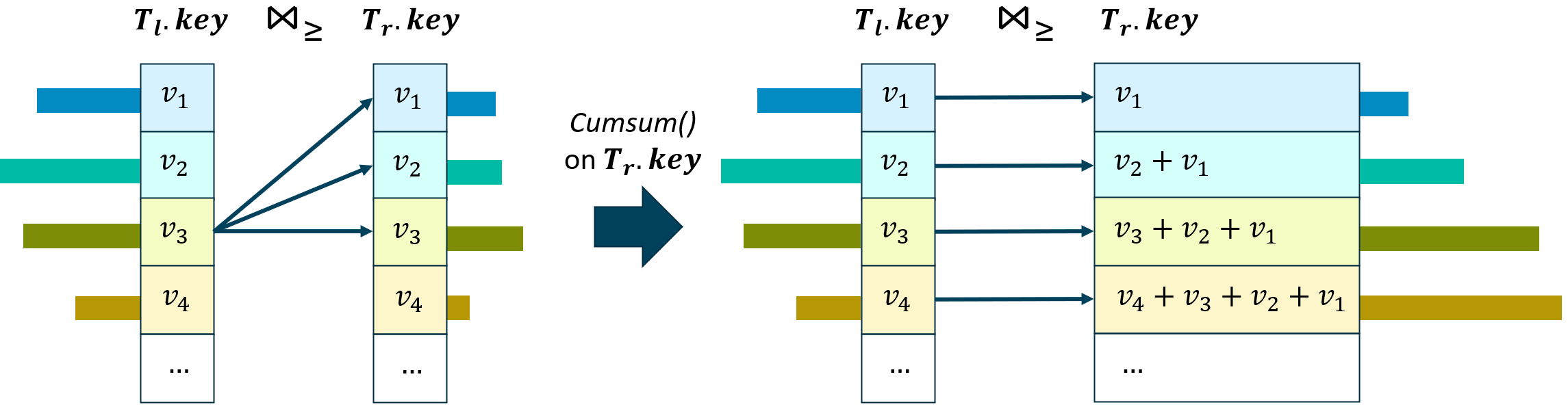
Figure 5: Illustration of DistJoin’s approach to calculating non-equi joins.

Input: Join type: $join\_how$, probability distributions: $\hat{\mathbf{P}}_{\mathcal{T}_{left}}(KEY,\mathcal{Q}),\hat{\mathbf{P}}_{\mathcal{T}_{right}}(KEY,\mathcal{Q}),\hat{\mathbf{P}}_{\mathcal{T}_{left}}(KEY),\hat{\mathbf{P}}_{\mathcal{T}_{right}}(KEY)$

Output: $\hat{\mathbf{P}}_{\mathcal{T}}(KEY,\mathcal{Q})$

1 $p_{l}(\mathcal{Q}),p_{r}(\mathcal{Q}),p_{l},p_{r}\longleftarrow\hat{\mathbf{P}}_{\mathcal{T}_{left}}(KEY,\mathcal{Q}),\hat{\mathbf{P}}_{\mathcal{T}_{right}}(KEY,\mathcal{Q}),\hat{\mathbf{P}}_{\mathcal{T}_{left}}(KEY),\hat{\mathbf{P}}_{\mathcal{T}_{right}}(KEY)$;

2 if $join\_how=^{\prime}\geq^{\prime}$ then

3    $p_{r}(\mathcal{Q})\longleftarrow\text{cumsum}(p_{r}(\mathcal{Q}))$ ;

4   

5 if $join\_how=^{\prime}\leq^{\prime}$ then

6    $p_{l}(\mathcal{Q})\longleftarrow\text{cumsum}(p_{l}(\mathcal{Q}))$ ;

7   

8 if $join\_how=^{\prime}>^{\prime}$ then

9    $p_{r}(\mathcal{Q})\longleftarrow\text{Roll}(p_{r}(\mathcal{Q}),1)$ ; //Circularly shift right one position

10    $p_{r}(\mathcal{Q})[0]\longleftarrow 0;$

11    $p_{r}(\mathcal{Q})\longleftarrow\text{cumsum}(p_{r}(\mathcal{Q}))$ ;

12   

13 if $join\_how=^{\prime}<^{\prime}$ then

14    $p_{l}(\mathcal{Q})\longleftarrow\text{Roll}(p_{l}(\mathcal{Q}),1)$ ; //Circularly shift right one position

15    $p_{l}(\mathcal{Q})[0]\longleftarrow 0;$

16    $p_{l}(\mathcal{Q})\longleftarrow\text{cumsum}(p_{l}(\mathcal{Q}))$ ;

17   

18 $\hat{\mathbf{P}}_{\mathcal{T}}(KEY,\mathcal{Q})\longleftarrow\frac{p_{l}(\mathcal{Q})\odot p_{r}(\mathcal{Q})}{\sum_{v}p_{l}\cdot p_{r}}$ ;

19

20return $\hat{\mathbf{P}}_{\mathcal{T}}(KEY,\mathcal{Q})$;

Algorithm 2 Inference of Join Cardinality for Different Join Conditions

Non-equi joins typically achieve higher accuracy than equi joins due to each source key having more target keys to join, resulting in higher selectivity. The cumsum operation virtually eliminates the possibility of serious underestimation caused by incorrectly estimating a key’s probability as 0, except for the first join key value during cumsum calculation.

7 Experiments

This section presents a comprehensive evaluation of DistJoin against common baselines.

7.1 Experimental Setting

Datasets & Workloads. We evaluate DistJoin’s performance using the IMDB dataset with JOB-light and JOB-light-ranges workloads, the most widely adopted benchmarks in cardinality estimation research. Given the lack of established workloads for learning-based cardinality estimators on non-equi joins, we extended JOB-light and JOB-light-ranges by replacing join conditions with non-equi joins and recalculating true cardinalities. Table 2 and Table 3 present statistical information demonstrating these benchmarks’ wide scenario coverage. As shown in Table 2, the dataset exhibits diverse column numbers, types, and NDV ranges. Additionally, we constructed a pre-updated dataset by randomly sampling $80\%$ of tuples from each table, simulating pre-update conditions for data and model update evaluations.

Table 3 and Figure 6 reveal that the $10$ test workloads cover extensive ranges of query true cardinality and join schema cardinality. Notably, JOB-light-ranges’ non-equi joins exhibit approximately 4 orders of magnitude lower selectivity, presenting greater prediction challenges. Non-equi joins demonstrate significantly higher true cardinality, with the six tables’ Cartesian product cardinality reaching $1.5e46$ - 13 orders of magnitude above the maximum $\text{card}_{J(\mathcal{T})}$. Consistent with subsection 6.3’s findings, we anticipate DistJoin’s superior performance over FactorJoin. The JOB-light workload with non-equi operators shows substantially higher true cardinality ranges due to simpler predicates, effectively demonstrating query-driven baselines like MSCN’s numerical challenges with non-equi joins.

Table 2: Statistical information of tables in the IMDB dataset included in our workloads. $\mathcal{C}$ represents for categorical type and $\mathcal{N}$ represents for numerical type.

	#Rows	#Columns	Column Types	NDV Range
cast info	360M	7	$\mathcal{C},\mathcal{N}$	11–23M
movie companies	26M	5	$\mathcal{C},\mathcal{N}$	660K–2.6M
movie info	140M	5	$\mathcal{C},\mathcal{N}$	71–140M
movie info idx	13M	5	$\mathcal{C},\mathcal{N}$	5–13M
movie keyword	45M	3	$\mathcal{C}$	470K–45M
title	25M	12	$\mathcal{C},\mathcal{N}$	1–25M

Table 3: Workloads statistical information.

	#Columns	#Predicates	Feature	Join	Cardinality Range	$\text{Card}_{J(\mathcal{T})}$ Range
JOB-light	8	1–5	basic joins	=	9–9.5e9	4.1e6–6.7e11
				$>$	7.6e10–4.0e30	4.7e13–4.7e32
				$<$	2.8e10–7.5e31	4.4e13–1.1e33
				$\geq$	7.6e10–4.0e30	4.7e13–4.7e32
				$\leq$	2.8e10–7.5e31	4.4e13–1.1e33
JOB-light-ranges	13	3–6	+complex predicates	=	1–2.3e11	4.1e6–6.7e11
				$>$	1.6e4–3.9e31	4.7e13–4.7e32
				$<$	5.0e4–1.3e32	4.4e13–1.1e33
				$\geq$	1.6e4–3.9e31	4.7e13–4.7e32
				$\leq$	5.0e4–1.3e32	4.4e13–1.1e33

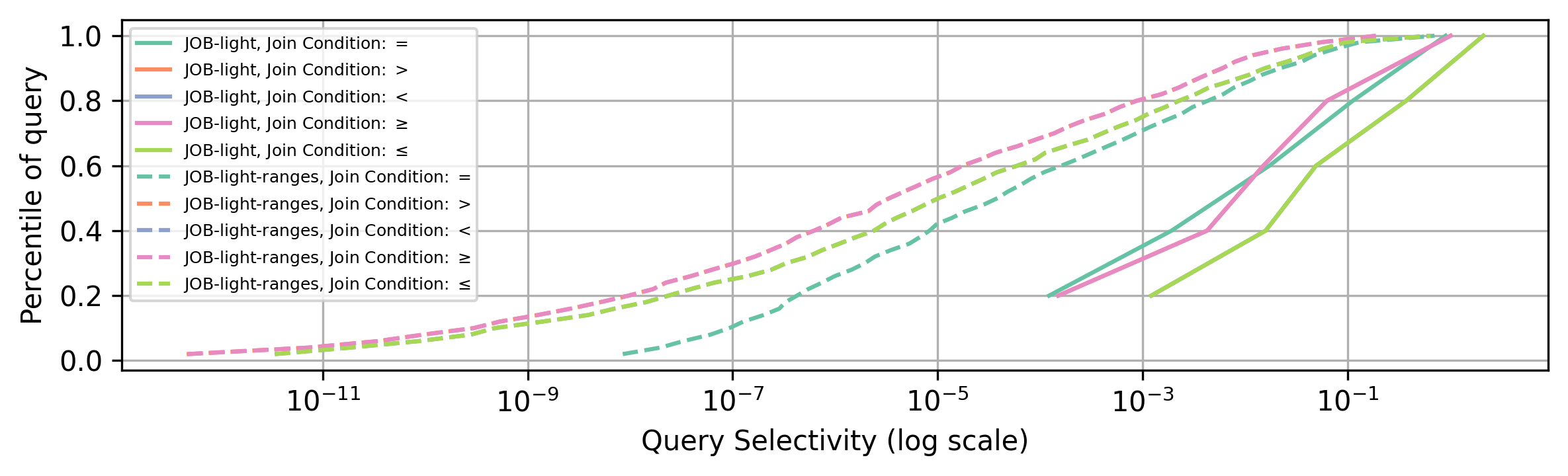
Figure 6: Distribution of each workload. The join conditions $(>,\geq)$ and $(<,\leq)$ have very similar selectivity distribution, so their curves overlay each other.

Baselines. We evaluate against the following baselines, covering conventional, data-driven, and query-driven methods:

1. PG: PostgreSQL (PG) , an open-source database with one of the most accurate traditional cardinality estimators, serves as a common baseline. We obtain estimated cardinality using the SQL template: "EXPLAIN (ANALYZE OFF) SELECT * FROM tables WHERE join_conditions AND predicates;".

2. NeuroCard: NeuroCard [49], a data-driven method based on a single autoregressive model trained on full outer join view samples, cannot support non-equi joins due to its dependence on fan-out values and full outer joins. We use the paper’s open-source code for evaluation.

3. MSCN: MSCN [19], a classic query-driven method and common baseline, theoretically supports non-equi joins but faces numerical challenges from typically higher non-equi join cardinalities. Despite mitigation efforts, including logarithmic transformation and Min-Max normalization, these issues persist. The training set combines MSCN’s synthetic workloads with 10K randomly generated queries containing both equi and non-equi joins. Evaluation uses the paper’s open-source code.

4. FactorJoin: FactorJoin [47], a data-driven method employing Bayesian Networks to estimate binned join key value probabilities under given predicates and using Equation 3 for join cardinality inference, cannot support non-equi joins due to its binning technique. Evaluation uses the paper’s open-source code.

We employ recommended settings from each baseline’s ‘readme’ files, optimized by their respective authors.

Metric. Following most cardinality estimation methods [14, 50, 49, 19, 42, 54, 17], we use Q-Error [31] to evaluate accuracy, an effective measure for CE problems [43]:

$$\text{Q-Error}=\frac{\max{(estimate,actual)}}{\min{(estimate,actual)}}$$ (79)

Model Architectures. Each table’s ANPM model includes:

• ResMADE with 4 layers (256 units each)

• ANPM HyperNetworks with 2 layers

• Factorized value bit width: 12

• Predicate embedding size: 64

Hardware. All experiments run on a PC with:

• CPU: AMD Ryzen9 7950X3D

• RAM: 32GB$\times 2$

• GPU: NVIDIA RTX4070Ti (12GB VRAM)

7.2 Accuracy Evaluation

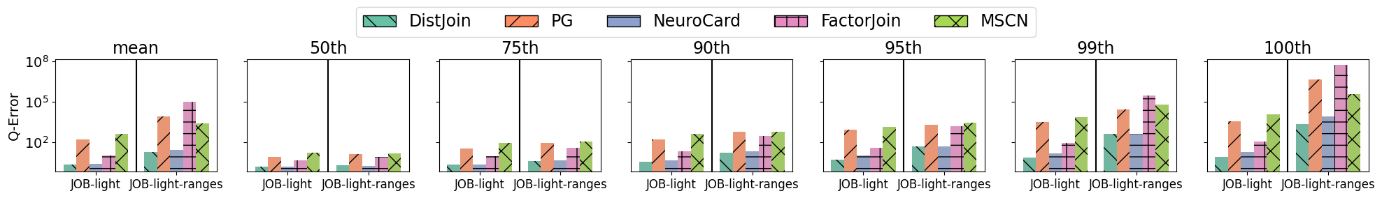
(a) Q-Error Percentiles by method, Join Condition:$=$

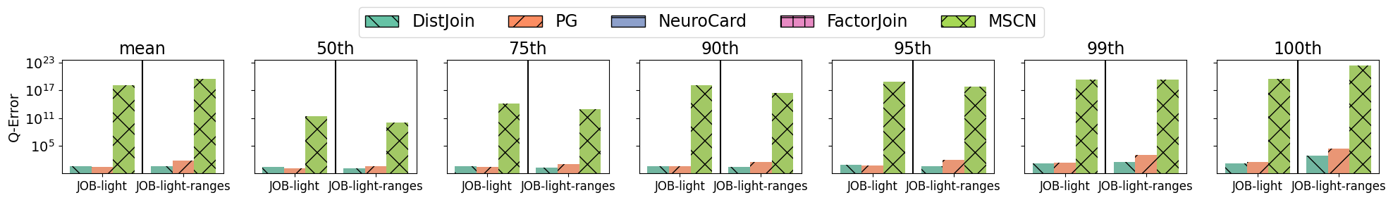
(b) Q-Error Percentiles by method, Join Condition:$>$

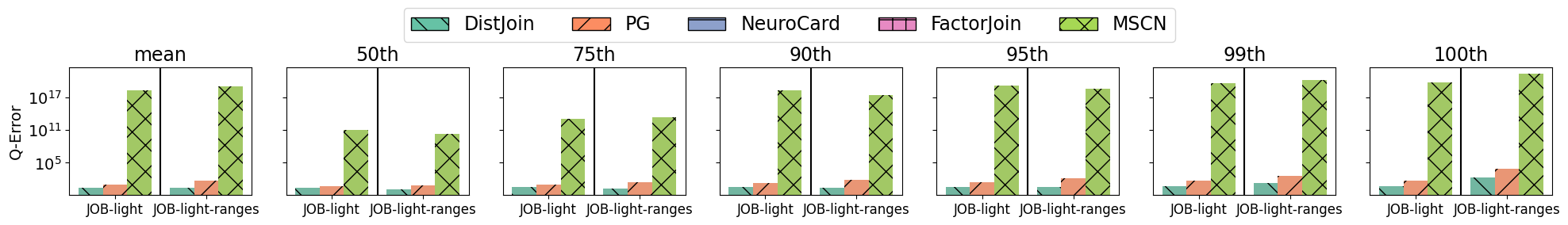
(c) Q-Error Percentiles by method, Join Condition:$<$

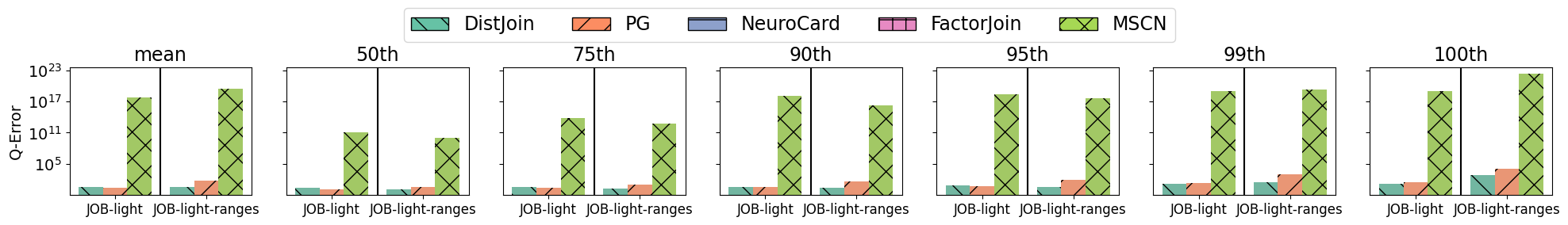
(d) Q-Error Percentiles by method, Join Condition:$\geq$

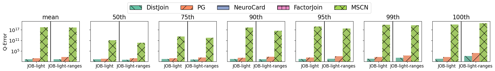
(e) Q-Error Percentiles by method, Join Condition:$\leq$

Figure 7: Overall Q-Error comparison for all methods.

We first compare DistJoin’s accuracy with baselines. Results appear in Table 4, Table 5, Table 6, and Figure 7. Note that while estimated cardinality differs between ($>$,$\geq$) and ($<$,$\leq$), their q_error values diverge only beyond the fourth decimal place (except for MSCN). To avoid redundancy, we exclude $\geq$ and $\leq$ results from tables. Figure 7 provides a comprehensive, intuitive comparison across all five join methods.

From these results, we draw the following conclusions:

1. DistJoin outperforms baselines on most Q-Error percentiles. Exceptions include: (1) NeuroCard’s slightly lower 50th percentile Q-Error on both workloads under equi joins; (2) PG’s lower mean, 50th, and 95th percentile Q-Errors on JOB-light with $>$ and $\geq$ joins. However, DistJoin demonstrates significantly lower Q-Errors in other scenarios. Notably, DistJoin exhibits lower 99th percentile and maximum Q-Errors across all scenarios, indicating a less pronounced long-tail error distribution. Comparing DistJoin with FactorJoin validates our analysis in Theorem 1 and Theorem 2.

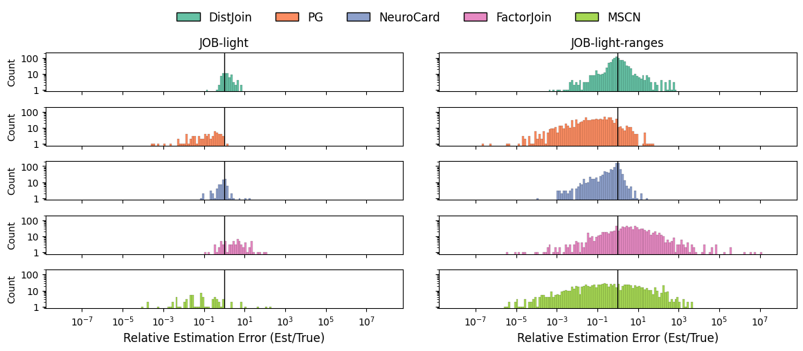
Figure 8: Distribution of the relative estimation error, which is the ratio between the estimated value and the true value and can be used for evaluating the bias of estimation.

2. DistJoin exhibits the lowest bias among baselines. As shown in Figure 8, DistJoin and NeuroCard show the lowest bias on JOB-light, while DistJoin alone achieves this on JOB-light-ranges. Although FactorJoin theoretically has lower bias, its binning technique amplifies bias by violating Assumption 1.

3. MSCN struggles with extreme true cardinality ranges. Its non-equi join Q-Errors significantly exceed other methods’. To investigate this and rule out adaptation errors, we conducted additional MSCN evaluations. We trained MSCN separately on its original synthetic workload (50K queries) and an expanded version with non-equi joins (250K queries total), ensuring full convergence over 100 epochs. As shown in Table 7, MSCN maintains normal accuracy on equi joins when trained on its synthetic workload but performs poorly on non-equi joins absent from training. Including non-equi joins in training significantly increases Q-Errors for both workloads with equi join conditions and increases Q-Errors’ long tail distribution for both workloads with non-equi join conditions, though the 50th percentile significantly improves for non-equi joins. This phenomenon cannot be attributed to labeling errors, as the results align well with PostgreSQL’s execution results. It is also not due to inconsistencies between the training and test workloads for non-equi joins, as both were processed using the same code. Such results suggest query-driven methods struggle with extreme true cardinality ranges due to training-test distribution mismatches. For instance, the extended synthetic workload’s maximum true cardinality ($6.9\times 10^{20}$) falls far short of JOB-light-ranges’ maximum ($1.3\times 10^{32}$) with $<$ joins. Generating matching training workloads for highly complex queries with enormous cardinalities proves extremely challenging, demonstrating query-driven methods’ practical limitations despite theoretical non-equi join support.

4. NeuroCard achieves slightly better median Q-Error but worse long-tail error distribution than DistJoin. We attribute this to NeuroCard’s training on full outer join view samples, which can span an enormous space [10], and those invalid tuples sampled during its progressive sampling process.

5. FactorJoin’s accuracy is constrained by its design. As the first method estimating join key distributions for join queries, FactorJoin made significant estimation compromises. Limited by BayesCard’s [48] estimation throughput, FactorJoin’s binning of join keys introduced additional errors, experimentally validating subsection 6.1’s variance analysis conclusions.

6. PG demonstrates limited scalability in handling non-equi join query complexity. While PG occasionally outperforms DistJoin on non-equi joins with fewer predicates (e.g., JOB-light with $>$ and $\geq$ joins), this performance is inconsistent. PG underperforms DistJoin on JOB-light with $<$ and $\leq$ joins and consistently trails DistJoin on the more complex, predicate-rich JOB-light-ranges workload.

In summary, the accuracy evaluation results demonstrate the previous methods’ limitations and DistJoin’s superiority in both generality and accuracy. DistJoin emerges as the only learned cardinality estimator effectively supporting non-equi joins among all baselines while achieving the highest accuracy in most scenarios.

Table 4: Q-Error comparison with Join Condition:$=$.

Methods	JOB-light					JOB-light-ranges
	mean	50th	95th	99th	max	mean	50th	95th	99th	max
PG	155.99	7.98	774.57	2879.3	3378.2	7618.3	13.24	1859.1	2.5e5	4.5e7
MSCN	402.46	15.74	1250.2	7340.1	1.1e5	2354.5	14.83	2694.8	6.0e5	3.8e6
NeuroCard	2.47	1.46	10.28	14.84	18.43	24.66	1.71	48.17	420.5	8169
FactorJoin	10.03	4.09	36.06	88.94	102.6	9.6e5	7.59	1514.5	2.9e6	5.7e8
DistJoin	1.99	1.49	4.53	6.92	7.63	18.76	1.88	47.22	388.66	2225.6

Table 5: Q-Error comparison with Join Condition:$>$.

Methods	JOB-light					JOB-light-ranges
	mean	50th	95th	99th	max	mean	50th	95th	99th	max
PG	2.58	1.34	6.16	21.99	30.54	63.7	3.82	90.47	1025.1	2.2e5
MSCN	1.2e18	2.7e12	8.0e18	2.3e19	2.9e19	2.6e19	1.2e11	5.7e17	2.2e19	2.5e22
DistJoin	3.24	2.82	7.26	16.26	16.67	4.13	1.35	4.28	35.32	762.4

Table 6: Q-Error comparison with Join Condition:$<$.

Methods	JOB-light					JOB-light-ranges
	mean	50th	95th	99th	max	mean	50th	95th	99th	max
PG	8.46	4.59	27.41	51.72	51.85	48.41	7.75	125.89	337.14	8566.6
MSCN	2.2e18	9.0e11	1.6e19	3.9e19	5.1e19	9.5e18	2.0e10	3.9e18	1.8e20	2.6e21
DistJoin	2.34	2.3	3.87	4.08	4.4	2.51	1.27	3.98	19.66	176.1

Table 7: Further evaluation of MSCN on JOB-light-ranges with its own Synthetic training workloads to rule out any adaption errors.

Train Workloads	Loss	Join	mean	50th	95th	99th	max
MSCN’s own Synthetic (w/o non-equi joins)	0.32	$=$	362.8	11.20	441.9	4304.9	1.1e6
		$>$	1.6e22	4.6e15	1.9e22	2.8e23	4.1e24
		$<$	7.6e22	5.7e15	8.8e22	1.8e24	9.2e24
MSCN’s own Synthetic + extended non-equi	0.29	$=$	4.5e8	1722.0	1.9e8	3.1e9	1.5e11
		$>$	5.6e28	1538.9	5.9e22	2.7e29	3.9e31
		$<$	5.7e29	1027.6	7.6e29	1.1e31	1.3e32

7.3 Speed of Update and Inference

Having demonstrated DistJoin’s generality and accuracy regarding the "Trilemma of Cardinality Estimation" in subsection 7.2, we now evaluate its update and inference speed against baselines.

For update speed, MSCN requires collecting training workload true cardinalities, NeuroCard needs full-outer join view samples, and FactorJoin must first apply its binning strategy to updated data. While MSCN and NeuroCard require complete retraining after data updates, FactorJoin theoretically only needs bucket updates rather than complete rebuilding. However, since this approach remains unimplemented in its code, we present its cold-start time alongside other methods. This limitation doesn’t affect FactorJoin’s status as the fastest updating method. Notably, DistJoin requires only distinct value sorting and encoding for data pre-processing, with training samples generated dynamically during training.

As shown in Table 8, FactorJoin achieves the fastest training and updating times, though its cold-start time is relatively longer due to binning. Proper optimization (e.g., replacing Python with C++) may significantly reduce pre-processing time. DistJoin ranks second in update speed, with its longest training time (309.7 seconds) occurring on the high-cardinality cast info table. NeuroCard trains quickly but requires 150 seconds for full-outer join view sampling, limiting scalability. Additionally, its database-coupled model prevents flexible updates when only some tables change. MSCN’s data annotation time exceeds 7 hours, making it nearly impractical for scenarios with frequent data updates and workload shifts.

Regarding inference time, MSCN’s simple design makes it the fastest, though its high Q-Error diminishes this advantage. DistJoin’s inference time is approximately $2\times$ FactorJoin’s, a worthwhile tradeoff given its significant accuracy improvements. NeuroCard’s inference time exceeds DistJoin’s by over $5\times$ while delivering higher Q-Errors.

In terms of model size, DistJoin’s models are significantly larger than others. As an autoregressive-based method, DistJoin’s ANPM models are much larger than FactorJoin’s BayesCard. Maintaining separate models for each table also makes DistJoin’s storage requirements much higher than NeuroCard’s. However, this storage overhead remains well below database systems’ maximum tolerable limits, imposing no storage pressure or compromising practicality.

Regarding GPU memory overhead, DistJoin requires more GPU memory than baselines during training. This stems from DistJoin’s individual table estimators employing the same training framework as our previous work, Duet [52]. Training on more predicate samples helps reduce long-tail error distribution effects, prompting us to use a batch size of $16384$ to maximize training throughput, resulting in higher GPU memory overhead. However, during inference, DistJoin’s GPU memory overhead is lower than NeuroCard’s.

Table 8: Performance comparison including time and memory costs on JOB-light-ranges with $=$ join condition. Since FactorJoin and DistJoin decouple models from the full outer join and maintain independent models per table, their models train separately. We show maximum metric values across all tables for comparison since they will be the performance bottleneck during training. For methods requiring complex pre-processing, we represent time as prepare time + training time.

	MSCN	NeuroCard	FactorJoin	DistJoin
Training Time	7 h+351.8 s	150.31+293.34 s	531.9+8.0 s	309.7 s
Training GPU Memory Cost	2.47 GB	4.49 GB	2.23 GB	6.49 GB
Inference Time per query	0.5 ms	60.61 ms	8.97 ms	17.96 ms
Inference GPU Memory Cost	2.27 GB	4.34 GB	2.18 GB	3.66 GB
Total Models’ Size	5.3 MB	6.4 MB	2.3 MB	56.1 MB

We illustrate DistJoin’s convergence curve in Figure 9. Since all tables train in parallel, grouping models by epoch proves difficult. Instead, we use the longest training time among all tables per epoch as the x-axis to demonstrate DistJoin’s performance convergence over 20 epochs. DistJoin converges quickly in terms of median metrics, suggesting that for scenarios less sensitive to long-tail error distributions, training time can be reduced by accepting slightly increased long-tail error distributions for faster training.

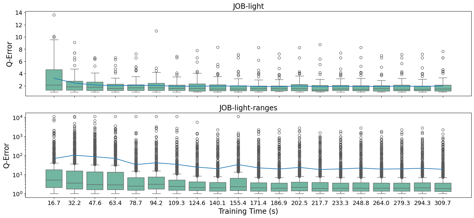
Figure 9: DistJoin’s convergence curve according to training time.

7.4 Robustness on Data Updating

This subsection evaluates DistJoin’s robustness against baselines. We simulate a pre-update dataset by randomly sampling 80% of tuples from each table, train all methods on this dataset, and evaluate them on both pre-update and updated workloads. Results appear in Figure 10.

For equi joins, DistJoin maintains the lowest Q-Error across all workload combinations. The last row of results, showing training on the pre-update dataset and evaluation on updated workloads, demonstrates DistJoin’s superior robustness compared to baselines. For non-equi joins, DistJoin and PG show competitive performance on JOB-light under different join conditions, with each outperforming the other in specific scenarios. However, on JOB-light-ranges, DistJoin significantly outperforms PG. MSCN exhibits substantially higher errors across both workloads.

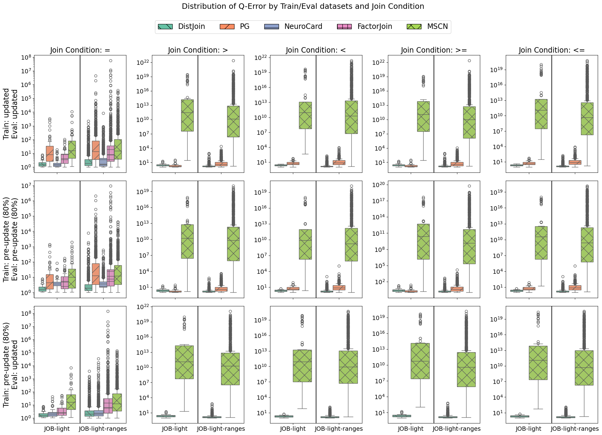
Figure 10: Q-Error comparison by workloads and join conditions to evaluate data update situation and robustness.

7.5 Ablation Study

This section validates the ANPM model’s effectiveness through an ablation study on workloads with equi join:

(A) Removing ANPM Blocks significantly increases Q-Error, proving ANPM’s effectiveness in improving accuracy.

(B) Removing the SOS and right-shift mechanism further increases Q-Error compared to (A).

(C) Removing the learnable softmax temperature coefficient significantly increases JOB-light’s maximum Q-Error while slightly decreasing other Q-Error metrics. Further investigation reveals that JOB-light includes equality predicates on highly skewed columns, and the filtered values’ count is very small, demonstrating the learnable temperature’s effectiveness in handling skewed columns at the cost of slight accuracy reductions in other scenarios. Thus, enabling this feature selectively for skewed columns is optimal.

(D) Removing the mixed activation function improves performance across all scenarios. To further study the effect of it, we applied an extra ablation study (E) by removing only the mixed activation function from the base model to explore how its interaction with other features affects model accuracy. The result shows a slight improvement in JOB-light maximum Q-Error with significant decreases in other Q-Error metrics. This indicates that the mixed activation function should be used in conjunction with all three other features to enhance the model performance in most scenarios.

Table 9: Ablation study of DistJoin’s model improvements on join condition $=$.

	ANPM Block	SOS +Right-shift	Learnable Temperature	Mixed Activation	JOB-light		JOB-light-ranges
					50th	max	50th	max
base	✓	✓	✓	✓	1.49	7.63	1.88	2225.6
(A)		✓	✓	✓	1.69	18.85	3.31	2e5
(B)			✓	✓	1.80	19.09	3.37	2.6e5
(C)				✓	1.71	128.1	3.14	1.4e5
(D)					1.60	125.9	2.87	1.5e5
(E)	✓	✓	✓		1.84	6.97	2.10	3709.3

8 Related Works

8.1 Conventional Cardinality Estimators

Conventional cardinality estimators primarily encompass histogram-based [2, 16, 26, 32, 36, 39, 40, 5], sample-based [1, 7, 9, 24, 37], and sketch-based [21] approaches. These methods aim to construct a simplified representation of the data to accurately capture its distribution. However, due to the complexity of dependencies both within and between tables, traditional methods often suffer from low accuracy. The advantage of such methods lies in their typically lightweight nature and ease of updating.

8.2 Learned Cardinality Estimators

Learned cardinality estimators can be categorized into three major types:

• Query-driven methods. Query-driven methods [4, 19, 34, 23, 20, 35, 38, 45] are based on supervised learning, thus, they generally support the widest range of query types. However, they require substantial time to collect training workloads, and most of them struggle to adapt to the workload drifting problem. In recent years, some pre-trained-based methods have been proposed [25, 51], which are significantly more robust than previous methods. Nevertheless, these methods demand even more time to label training workloads.

• Data-driven methods. Data-driven methods learn from the data itself rather than the queries. The SPN-based methods [14, 54] utilize sum-product networks to model the data distribution and employ fan-out values to estimate join queries. The autoregressive-based methods [50, 49, 52, 42, 17, 48, 47] use autoregressive models to predict the probability distribution of tables. Many of these methods [50, 52, 42, 48] focus on single-table queries. However, recent studies [49, 47, 17] have shifted towards supporting join queries. For instance, NeuroCard [49] supports equi joins by learning from the full outer join view, and FactorJoin [47] supports multi-key equi joins by binning the join keys and predicting the bin size with BayesCard [48]. ASM [17] extends NeuroCard [49]’s progressive sampling and estimates equi joins by predicting the sample’s multi-dimensional probability distributions. However, none of these methods consider non-equi joins.

• Hybrid methods. Hybrid methods [46, 52] are based on both supervised and unsupervised learning. UAE [46] achieves hybrid training by enhancing Naru [50]’s progressive sampling method and making it differentiable. Duet [52] is a single-table estimator that supports both data-driven and hybrid training modes. It accomplishes this by estimating the data distribution under given predicates, thereby eliminating the non-differentiable sampling process of Naru.

8.3 Autoregressive Model

The autoregressive model is a type of unsupervised model that learns the data distribution. MADE [6] and its enhanced version, ResMADE [33], are the simplest autoregressive models, composed of a partially connected neural network with carefully designed masks and linear layers. They are highly efficient in explicit density estimation. RNN networks [15, 3] are a classic type of autoregressive model commonly used in time series data analysis. Transformer [41] is the most well-known autoregressive network, which enforces autoregressive constraints between inputs and outputs through causal masking. It is widely used in NLP tasks and can also perform explicit density estimation. However, it incurs higher computational costs and does not always demonstrate significant performance advantages over MADE in small-scale scenarios [50].

9 Conclusion

In this paper, we introduce Adaptive Neural Predicate Modulation (ANPM), a novel autoregressive model, and present DistJoin, a decoupled join cardinality estimation framework built upon ANPM. Benefiting from the efficient probability estimation capability and strong scalability of ANPM, DistJoin effectively addresses the "Trilemma of Cardinality Estimation" problem, achieving superior performance across three dimensions: generality, accuracy, and updatability, thereby demonstrating enhanced practicality. DistJoin leverages a decoupled selectivity-based join cardinality inference approach to reason about the probability distributions estimated by ANPM, enabling effective support for non-equi joins for the first time among data-driven methods. Furthermore, through theoretical analysis and experiments, we demonstrate that the join cardinality inference method used in prior similar approaches [47] suffers from limited scalability, while the selectivity-based join cardinality inference proposed and utilized in DistJoin is proven to be unbiased under given assumptions, with variance growing more slowly as the join size increases. Experimental results show that DistJoin significantly outperforms baselines in estimation accuracy, robustness, and generality while maintaining flexible updates and efficient inference, validating its practicality. Finally, ablation studies confirm the effectiveness of the series of improvements proposed in ANPM.

Declaration of generative AI and AI-assisted technologies in the writing process

During the preparation of this work the author(s) used DeepSeek in order to improve language readability and correct grammatical errors. After using this tool/service, the author(s) reviewed and edited the content as needed and take(s) full responsibility for the content of the publication.

References

- Charikar et al. [2000] Charikar, M., Chaudhuri, S., Motwani, R., Narasayya, V.R., 2000. Towards estimation error guarantees for distinct values. Proceedings of the nineteenth ACM SIGMOD-SIGACT-SIGART symposium on Principles of database systems URL: https://api.semanticscholar.org/CorpusID:345658.
- Deshpande et al. [2001] Deshpande, A., Garofalakis, M.N., Rastogi, R., 2001. Independence is good: dependency-based histogram synopses for high-dimensional data, in: ACM SIGMOD Conference. URL: https://api.semanticscholar.org/CorpusID:10162308.
- Dey and Salem [2017] Dey, R., Salem, F.M., 2017. Gate-variants of gated recurrent unit (gru) neural networks, in: 2017 IEEE 60th International Midwest Symposium on Circuits and Systems (MWSCAS), pp. 1597–1600. doi:10.1109/MWSCAS.2017.8053243.
- Dutt et al. [2019] Dutt, A., Wang, C., Nazi, A., Kandula, S., Narasayya, V.R., Chaudhuri, S., 2019. Selectivity estimation for range predicates using lightweight models. Proc. VLDB Endow. 12, 1044–1057. URL: https://api.semanticscholar.org/CorpusID:195735541.
- Gelder [1993] Gelder, A.V., 1993. Multiple join size estimation by virtual domains (extended abstract). Proceedings of the twelfth ACM SIGACT-SIGMOD-SIGART symposium on Principles of database systems URL: https://api.semanticscholar.org/CorpusID:209399043.
- Germain et al. [2015] Germain, M., Gregor, K., Murray, I., Larochelle, H., 2015. Made: Masked autoencoder for distribution estimation. ArXiv abs/1502.03509. URL: https://api.semanticscholar.org/CorpusID:1399080.
- Gibbons [2001] Gibbons, P.B., 2001. Distinct sampling for highly-accurate answers to distinct values queries and event reports, in: Very Large Data Bases Conference. URL: https://api.semanticscholar.org/CorpusID:1516032.
- Goodfellow et al. [2016] Goodfellow, I., Bengio, Y., Courville, A., 2016. Deep Learning. MIT Press. http://www.deeplearningbook.org.
- Haas et al. [1994] Haas, P.J., Naughton, J.F., Swami, A.N., 1994. On the relative cost of sampling for join selectivity estimation. Proceedings of the thirteenth ACM SIGACT-SIGMOD-SIGART symposium on Principles of database systems URL: https://api.semanticscholar.org/CorpusID:7218721.
- Han et al. [2021] Han, Y., Wu, Z., Wu, P., Zhu, R., Yang, J., Tan, L.W., Zeng, K., Cong, G., Qin, Y., Pfadler, A., Qian, Z., Zhou, J., Li, J., Cui, B., 2021. Cardinality estimation in dbms: A comprehensive benchmark evaluation. Proc. VLDB Endow. 15, 752–765. URL: https://api.semanticscholar.org/CorpusID:237490370.
- Harmouch and Naumann [2017] Harmouch, H., Naumann, F., 2017. Cardinality estimation: An experimental survey. Proc. VLDB Endow. 11, 499–512. URL: https://api.semanticscholar.org/CorpusID:6744919.
- Hendrycks and Gimpel [2023] Hendrycks, D., Gimpel, K., 2023. Gaussian error linear units (gelus). URL: https://arxiv.org/abs/1606.08415, arXiv:1606.08415.
- Hilprecht and Binnig [2022] Hilprecht, B., Binnig, C., 2022. Zero-shot cost models for out-of-the-box learned cost prediction. Proc. VLDB Endow. 15, 2361–2374. URL: https://doi.org/10.14778/3551793.3551799, doi:10.14778/3551793.3551799.
- Hilprecht et al. [2020] Hilprecht, B., Schmidt, A., Kulessa, M., Molina, A., Kersting, K., Binnig, C., 2020. Deepdb: Learn from data, not from queries!, VLDB Endowment. pp. 992–1005.
- Hochreiter and Schmidhuber [1997] Hochreiter, S., Schmidhuber, J., 1997. Long short-term memory. Neural Comput. 9, 1735–1780. URL: https://doi.org/10.1162/neco.1997.9.8.1735, doi:10.1162/neco.1997.9.8.1735.
- Jagadish et al. [2001] Jagadish, H.V., Jin, H., Ooi, B.C., Tan, K.L., 2001. Global optimization of histograms, in: ACM SIGMOD Conference. URL: https://api.semanticscholar.org/CorpusID:52857204.
- Kim et al. [2024] Kim, K., Lee, S., Kim, I., Han, W.S., 2024. Asm: Harmonizing autoregressive model, sampling, and multi-dimensional statistics merging for cardinality estimation. Proc. ACM Manag. Data 2. URL: https://doi.org/10.1145/3639300, doi:10.1145/3639300.
- Kingma and Ba [2017] Kingma, D.P., Ba, J., 2017. Adam: A method for stochastic optimization. URL: https://arxiv.org/abs/1412.6980, arXiv:1412.6980.
- Kipf et al. [2018a] Kipf, A., Kipf, T., Radke, B., Leis, V., Boncz, P.A., Kemper, A., 2018a. Learned cardinalities: Estimating correlated joins with deep learning. ArXiv abs/1809.00677. URL: https://api.semanticscholar.org/CorpusID:52154172.
- Kipf et al. [2018b] Kipf, A., Kipf, T., Radke, B., Leis, V., Boncz, P.A., Kemper, A., 2018b. Learned cardinalities: Estimating correlated joins with deep learning. ArXiv abs/1809.00677. URL: https://api.semanticscholar.org/CorpusID:52154172.
- Kumar et al. [2004] Kumar, A., Xu, J., Wang, J., Spatscheck, O., Li, E.L., 2004. Space-code bloom filter for efficient per-flow traffic measurement. IEEE INFOCOM 2004 3, 1762–1773 vol.3. URL: https://api.semanticscholar.org/CorpusID:1438136.
- Larson et al. [2007] Larson, P.Å., Lehner, W., Zhou, J., Zabback, P., 2007. Cardinality estimation using sample views with quality assurance, in: ACM SIGMOD Conference. URL: https://api.semanticscholar.org/CorpusID:2694333.
- Li et al. [2023] Li, P., Wei, W., Zhu, R., Ding, B., Zhou, J., Lu, H., 2023. Alece: An attention-based learned cardinality estimator for spj queries on dynamic workloads. Proc. VLDB Endow. 17, 197–210. URL: https://doi.org/10.14778/3626292.3626302, doi:10.14778/3626292.3626302.
- Lipton et al. [1990] Lipton, R.J., Naughton, J.F., Schneider, D.A., 1990. Practical selectivity estimation through adaptive sampling, in: ACM SIGMOD Conference. URL: https://api.semanticscholar.org/CorpusID:5368912.
- Lu et al. [2021] Lu, Y., Kandula, S., König, A.C., Chaudhuri, S., 2021. Pre-training summarization models of structured datasets for cardinality estimation. Proc. VLDB Endow. 15, 414–426. URL: https://api.semanticscholar.org/CorpusID:245999750.
- Lynch [1988] Lynch, C.A., 1988. Selectivity estimation and query optimization in large databases with highly skewed distribution of column values, in: Very Large Data Bases Conference. URL: https://api.semanticscholar.org/CorpusID:20418479.
- Ma et al. [2021] Ma, L., Zhang, W., Jiao, J., Wang, W., Butrovich, M., Lim, W.S., Menon, P., Pavlo, A., 2021. Mb2: Decomposed behavior modeling for self-driving database management systems, in: Proceedings of the 2021 International Conference on Management of Data, Association for Computing Machinery, New York, NY, USA. p. 1248–1261. URL: https://doi.org/10.1145/3448016.3457276, doi:10.1145/3448016.3457276.
- Marcus et al. [2021] Marcus, R., Negi, P., Mao, H., Tatbul, N., Alizadeh, M., Kraska, T., 2021. Bao: Making learned query optimization practical, in: Proceedings of the 2021 International Conference on Management of Data, Association for Computing Machinery, New York, NY, USA. p. 1275–1288. URL: https://doi.org/10.1145/3448016.3452838, doi:10.1145/3448016.3452838.
- Marcus et al. [2019] Marcus, R., Negi, P., Mao, H., Zhang, C., Alizadeh, M., Kraska, T., Papaemmanouil, O., Tatbul, N., 2019. Neo: a learned query optimizer. Proc. VLDB Endow. 12, 1705–1718. URL: https://doi.org/10.14778/3342263.3342644, doi:10.14778/3342263.3342644.
- Marcus and Papaemmanouil [2019] Marcus, R., Papaemmanouil, O., 2019. Plan-structured deep neural network models for query performance prediction. ArXiv abs/1902.00132. URL: https://api.semanticscholar.org/CorpusID:59553521.
- Moerkotte et al. [2009] Moerkotte, G., Neumann, T., Steidl, G., 2009. Preventing bad plans by bounding the impact of cardinality estimation errors. Proc. VLDB Endow. 2, 982–993. URL: https://api.semanticscholar.org/CorpusID:7132856.
- Muralikrishna and DeWitt [1988] Muralikrishna, M., DeWitt, D.J., 1988. Equi-depth multidimensional histograms, in: ACM SIGMOD Conference. URL: https://api.semanticscholar.org/CorpusID:209400290.
- Nash and Durkan [2019] Nash, C., Durkan, C., 2019. Autoregressive energy machines. ArXiv abs/1904.05626. URL: https://api.semanticscholar.org/CorpusID:119290776.
- Negi et al. [2023] Negi, P., Wu, Z., Kipf, A., Tatbul, N., Marcus, R., Madden, S., Kraska, T., Alizadeh, M., 2023. Robust query driven cardinality estimation under changing workloads. Proc. VLDB Endow. 16, 1520–1533. URL: https://api.semanticscholar.org/CorpusID:258190940.
- Ortiz et al. [2019] Ortiz, J., Balazinska, M., Gehrke, J., Keerthi, S.S., 2019. An empirical analysis of deep learning for cardinality estimation. ArXiv abs/1905.06425. URL: https://api.semanticscholar.org/CorpusID:155100270.
- Poosala et al. [1996] Poosala, V., Ioannidis, Y.E., Haas, P.J., Shekita, E.J., 1996. Improved histograms for selectivity estimation of range predicates, in: ACM SIGMOD Conference. URL: https://api.semanticscholar.org/CorpusID:2948277.
- Riondato et al. [2011] Riondato, M., Akdere, M., Çetintemel, U., Zdonik, S.B., Upfal, E., 2011. The vc-dimension of sql queries and selectivity estimation through sampling, in: ECML/PKDD. URL: https://api.semanticscholar.org/CorpusID:13986444.
- Sun and Li [2019] Sun, J., Li, G., 2019. An end-to-end learning-based cost estimator. Proc. VLDB Endow. 13, 307–319. URL: https://api.semanticscholar.org/CorpusID:174802790.
- Thaper et al. [2002] Thaper, N., Guha, S., Indyk, P., Koudas, N., 2002. Dynamic multidimensional histograms, in: ACM SIGMOD Conference. URL: https://api.semanticscholar.org/CorpusID:2184836.
- To et al. [2013] To, H., Chiang, K., Shahabi, C., 2013. Entropy-based histograms for selectivity estimation. Proceedings of the 22nd ACM international conference on Information & Knowledge Management URL: https://api.semanticscholar.org/CorpusID:933510.
- Vaswani et al. [2017] Vaswani, A., Shazeer, N., Parmar, N., Uszkoreit, J., Jones, L., Gomez, A.N., Kaiser, L., Polosukhin, I., 2017. Attention is all you need, in: Proceedings of the 31st International Conference on Neural Information Processing Systems, Curran Associates Inc., Red Hook, NY, USA. p. 6000–6010.
- Wang et al. [2021] Wang, J., Chai, C., Liu, J., Li, G., 2021. Face: A normalizing flow based cardinality estimator. Proc. VLDB Endow. 15, 72–84. URL: https://api.semanticscholar.org/CorpusID:244771794.
- Wang et al. [2020] Wang, X., Qu, C., Wu, W., Wang, J., Zhou, Q., 2020. Are we ready for learned cardinality estimation? ArXiv abs/2012.06743. URL: https://api.semanticscholar.org/CorpusID:229157499.
- Whang et al. [1990] Whang, K.Y., Zanden, B.T.V., Taylor, H.M., 1990. A linear-time probabilistic counting algorithm for database applications. ACM Trans. Database Syst. 15, 208–229. URL: https://api.semanticscholar.org/CorpusID:2939101.
- Wu et al. [2018] Wu, C., Jindal, A., Amizadeh, S., Patel, H., Le, W., Qiao, S., Rao, S., 2018. Towards a learning optimizer for shared clouds. Proc. VLDB Endow. 12, 210–222. URL: https://api.semanticscholar.org/CorpusID:58015526.
- Wu and Cong [2021] Wu, P., Cong, G., 2021. A unified deep model of learning from both data and queries for cardinality estimation. Proceedings of the 2021 International Conference on Management of Data URL: https://api.semanticscholar.org/CorpusID:235474251.
- Wu et al. [2023] Wu, Z., Negi, P., Alizadeh, M., Kraska, T., Madden, S., 2023. Factorjoin: A new cardinality estimation framework for join queries. Proc. ACM Manag. Data 1. URL: https://doi.org/10.1145/3588721, doi:10.1145/3588721.
- Wu et al. [2020] Wu, Z., Shaikhha, A., Zhu, R., Zeng, K., Han, Y., Zhou, J., 2020. Bayescard: Revitilizing bayesian frameworks for cardinality estimation. arXiv preprint arXiv:2012.14743 .
- Yang et al. [2020] Yang, Z., Kamsetty, A., Luan, S., Liang, E., Duan, Y., Chen, X., Stoica, I., 2020. Neurocard. Proceedings of the VLDB Endowment 14, 61 – 73. URL: https://api.semanticscholar.org/CorpusID:219687533.
- Yang et al. [2019] Yang, Z., Liang, E., Kamsetty, A., Wu, C., Duan, Y., Chen, X., Abbeel, P., Hellerstein, J.M., Krishnan, S., Stoica, I., 2019. Deep unsupervised cardinality estimation, VLDB Endowment. pp. 279–292.
- Zeng et al. [2024] Zeng, T., Lan, J., Ma, J., Wei, W., Zhu, R., Li, P., Ding, B., Lian, D., Wei, Z., Zhou, J., 2024. Price: A pretrained model for cross-database cardinality estimation. ArXiv abs/2406.01027. URL: https://api.semanticscholar.org/CorpusID:270215321.
- Zhang et al. [2024] Zhang, K., Wang, H., Lu, Y., Li, Z., Shu, C., Yan, Y., Yang, D., 2024. Duet: Efficient and Scalable Hybrid Neural Relation Understanding , in: 2024 IEEE 40th International Conference on Data Engineering (ICDE), IEEE Computer Society, Los Alamitos, CA, USA. pp. 56–69. URL: https://doi.ieeecomputersociety.org/10.1109/ICDE60146.2024.00012, doi:10.1109/ICDE60146.2024.00012.
- Zhao et al. [2022] Zhao, Y., Cong, G., Shi, J., Miao, C., 2022. Queryformer: a tree transformer model for query plan representation. Proc. VLDB Endow. 15, 1658–1670. URL: https://doi.org/10.14778/3529337.3529349, doi:10.14778/3529337.3529349.
- Zhu et al. [2021] Zhu, R., Wu, Z., Han, Y., Zeng, K., Pfadler, A., Qian, Z., Zhou, J., Cui, B., 2021. Flat: fast, lightweight and accurate method for cardinality estimation. Proc. VLDB Endow. 14, 1489–1502. URL: https://doi.org/10.14778/3461535.3461539, doi:10.14778/3461535.3461539.